To farm or not to farm? Indian farmers in transition - Cathie ...

www.gdi.manchester.ac.uk

Global Development Institute Working Paper Series: 001

To farm or not to farm?

Indian farmers in transition

Bina Agarwal1 and Ankush Agrawal2

1 Professor of Development Economics and Environment, Global Development

Institute, The University of Manchester, United Kingdom.

Email: [email protected]

2 Assistant Professor of Economics, Indian Institute of Technology Delhi, New

Delhi, India.

Email: [email protected]

April 2016

ISBN: 978-1-909336-35-3

www.gdi.manchester.ac.uk 2

Abstract

Few studies of agrarian transition examine what farmers themselves feel about farming. Are they

cultivating out of choice or a lack of options? What distinguishes farmers who like farming from those

who do not: their personal and household characteristics and endowments? The local ecology and

regional economy? Or a mix of these and other factors? Understanding farmer satisfaction is important

not only for assessing citizen well-being but also for agricultural productivity, since occupational

satisfaction can affect a farmer’s incentive to invest and reveal production constraints. Using a unique

all-India data set which asked farmers—do you like farming?—this paper provides answers and policy

pointers, contributing a little-studied dimension to debates on the smallholder’s future and subjective

well-being.

Keywords

Farmer satisfaction, agrarian transition, subjective well-being, production constraints, India

JEL Codes

N55, O12, O13

Acknowledgements

We thank Kunal Sen, Raghav Gaiha and Abhiroop Mukhopadhyay for their comments, and the

Leverhulme Trust for its support of Bina Agarwal’s time under its Major Research Fellowship.

The survey data used here is available through the open access website

(http://mospi.nic.in/Mospi_New/site/inner.aspx?status=3&menu_id=37). Supplementary data sources

are referenced in the paper.


1. Introduction

In large parts of the developing world, non-farm employment has grown much slower than additions to

the work force. Vast numbers are confined to agriculture not out of choice but from a lack of alternatives.

Although this can be surmised from indirect indicators, such as the large proportion of rural workers

globally who continue to live in poverty and depend on agriculture for a livelihood (Agarwal, 2014a), or

from farmer suicides in countries such as India (Mishra, 2006; Greure and Sengupta, 2011), rarely are

those involved in farming asked directly if they like their occupation; and if born into a farming family

whether they would like to continue or move out—if they had a choice?

In fact, today we see two contrasting and implicit assumptions in discussions on the future of farmers,

neither of which is based on a direct verification of what farmers themselves want: (i) the assumption in

emergent farmers’ movements that all farmers want to farm, and (ii) the assumption of many

governments that most farmers would be better-off in cities. An example of the former is the growing

food sovereignty movement which emphasizes farmers’ rights to be self-sufficient in food and, on that

premise, lobbies for their right to grow their own food.1 However, such premises ignore the difficulties

farmers often face, especially the millions that are small and marginal, in becoming food self-sufficient

or economically profitable. The movements also often fail to represent the interests or perspectives of

poorer farmers (Agarwal, 2014b; Borras, 2008). In contrast, governments of large countries such as

India and China are planning rapid urbanization, focusing on ‘smart cities’, and facilitating rural land

acquisitions which could displace millions of smallholders who have few skills beyond farming, on the

assumption that they will be better-off in cities, again without taking account of their own wishes.

A rare opportunity to examine what farmers themselves want is provided by an all-India survey of over

fifty thousand rural farm households carried out by the National Sample Survey Organisation (NSSO)

of India in 2003 (GoI, 2005a). This Situation Assessment Survey (SAS) posed a simple question to

those who were farming full time: ‘Do you like farming as a profession?’ A surprising 40 per cent said

they did not, and if given a choice would prefer another source of livelihood.

Who are these farmers? Are they resource constrained, indebted, unable to make a viable living from

farming? Or are they the educated and better-off who would prefer leaving agriculture if they had other

options? And what about the 60 per cent who said they liked farming? How do they differ from the 40

per cent who said they did not? Also, what reasons do those who disliked farming give for their view,

and how do these reasons compare with an objective assessment of their economic, personal and

locational characteristics?

The SAS data (dovetailed with other macro-data) provides a rare opportunity to answer such questions,

and understand what types of farmers dislike farming, and why. We believe this is the first country-wide

survey which gives voice to a population that rarely has voice or choice. We examine the socioeconomic

profile of these farmers, and whether dissatisfaction with farming bears any association with their

profiles. Drawing on additional data, we also examine to what extent the farmer’s geographic region—

its ecology, climate, prosperity, and related factors— impinges on how he/she feels about farming. To

our knowledge, no other study barring one (Birthal et al 2015) has tested farmer satisfaction on such a

large, representative sample. Even the Birthal et al study does not examine the effect of such a complex

range of variables as we have done: for instance, it does not analyse any factor beyond the farmer’s

own characteristics; and even vis-à-vis these characteristics it ignores the impact of gender, the source

1 La Via Campesina, the food sovereignty movement, is constituted of around 148 organizations across 69 countries (Martinez-Torres and Rosset 2010).


and season in which irrigation is available, and the sources of loans.2 Ours (apart from Birthal et al’s) is

also one of very few studies on farmer satisfaction for a developing country. The analysis will help us

assess the objective reasons for farmer dissatisfaction, and so identify policies for improving farming

conditions.

Although the SAS data relates to 2003, the question about farmer satisfaction remains as valid today,

given contemporary debates about the future of the smallholder, persisting rural poverty and inequality,

and the continuing uneven agrarian transition in most developing countries. Also this remains a unique

data set, since a repeat SAS survey in 2013 did not canvas questions on farmer perceptions.

Farmer satisfaction has an important bearing not only on the well-being of millions of Indian citizens

who are dependent on agriculture but also on agricultural growth, since it can impinge on a farmer’s

motivation to undertake long-term farm investment. If the dissatisfied farmers are mostly the

disadvantaged, our analysis can point to policy responses for overcoming their resource or social

constraints. If the dissatisfied farmers are the better-off or educated, other policy responses would be

relevant, or we might need a policy mix for both categories of farmers.

Our analysis will thus contribute to at least two ongoing debates. The first concerns the future of

smallholders. Some argue that small and marginal farms have a limited future and most should be

accommodated in the non-farm, especially urban sector (for example, Collier and Dercon, 2014). This

is also an important premise behind the earlier-mentioned efforts in countries such as India and China

to promote shifts of rural people to cities. But others challenge the logic of such trajectories,

demonstrating empirically that the best chance of poverty reduction is improvement within the farm

sector itself (Imai et al., 2014), and the non-viability of accommodating, in the immediate future, vast

numbers in urban areas, given the limited growth in non-farm employment and the expected additions

to the labour force (Binswanger-Mkhize, 2013; Himanshu et al., 2014).

The second debate concerns life or job satisfaction. Existing research relates largely to individual

developed countries, or to broad cross-country comparisons. Ravallion and Lokshin (2002), for

instance, study the determinants of self-rated well-being in Russia; Blanchflower and Oswald (2004) in

the USA and UK; and Bjornskov (2003) and Deaton (2008) in many countries globally. These studies

find that individual income is a significant predictor of happiness and life satisfaction. But is this also

true for all sections of a developing country’s population? And to what extent do locational or

environmental factors (rather than simply individual characteristics) matter? Similarly, several studies

on job satisfaction find that job security, pay, and the nature and hours of work are important

determinants. But these studies relate to formal sector jobs, mostly in developed countries (Clark, 2001)

and occasionally in developing ones (Mulinge and Mueller, 1998).

Our study locates itself largely within the first debate on the viability and future of smallholders and an

incomplete agrarian transition, while bringing to the second debate on job satisfaction the little-studied

perceptions of informal sector workers in a developing economy, as well as insights on both individual

and locational factors which impinge on these perceptions.

Below, we first discuss the literature on farmers’ self-perceptions and their decision or desire to exit

farming (Section 2). We then describe our dataset, theorise why particular factors might affect farmer

2 These authors have also omitted some 10,000 sample households, including those not owning land, which does not appear justified.


preferences, and present our results (Sections 3 and 4). Finally, we revisit the debate on the future of

the smallholder and present concluding reflections (Sections 5 and 6).

2. Existing studies

Existing research on farmers who want to quit farming but have not actually done so, is extremely

limited. Viira et al.’s (2010) study of Estonian farmers is among these few. Based on a 2007 postal

survey, it asked farmers about their intentions of quitting within three years. Farmers who diversified

into non-farm activities, owned rather than rented in most of their land, were in good health, had larger

farms, or were older even if operating small farms, were found less likely to want to quit. Farmers in

livestock production (which tends to be more capital and labour intensive) were more motivated to quit.

However, the study did not examine many other variables that could affect a farmer’s desire to quit,

such as his/her gender, access to credit, irrigation, and government support, and regional ecology and

economy.

Most other studies have a different focus—namely, on farmers who have already quit relative to those

who have not (see, Barkley, 1990; Bentley and Saupe, 1990; Kimhi, 2000; Goetz and Debertin, 2001;

Glauben et al., 2006). These studies are at best indicative of a farmer’s desire to quit, but tell us little

about that desire directly. Also, they focus on a few variables, especially the effect of non-farm

employment, which can go either way (see, Goetz and Debertin 2001 for the United States and Glauben

et al 2006 for West Germany). In addition, an early study (Gasson 1969) on the United Kingdom

examines whether farmer’s sons are more likely to take up farming, and finds that they are.

Importantly, whether focused on a farmer’s desire to quit, or on farmers who have already quit, there

are few studies on developing countries. Development literature on agrarian transitions focuses mostly

on aggregate shifts of people from farm to non-farm jobs, rather than on the farmers themselves.

Exceptions include Hye-Jung (2006) and Kang (2010) on Korea. Hye-Jung examined whether age and

farm size contributed to farmers leaving agriculture during 1998-2002 and found a non-linear

relationship. Kang examined government incentives for the youth to enter farming and older farmers to

leave it, and found that the young preferred lucrative non-farm options and older farmers preferred

continuing with farming.

At best, therefore, existing studies provide a window into only a few factors which impinge on a farmer’s

desire to continue (or leave) farming, and largely for developed countries. This leaves important gaps.

First, we know rather little about the farmer’s own likes vis-à-vis an occupation into which he/she has

typically been born, rather than chosen. This matters, since (as noted) dislike for the job could reduce

the incentive to invest in the land or seek new skills, and could thus adversely affect farm productivity.

Secondly, a wide range of factors could affect the farmers’ motivations, especially the constraints

he/she is subject to rather than a dislike for farming itself. This could include both individual constraints,

such as access to land, credit, inputs, extension services, and locational factors, such as the ecology,

climate, commercialisation, and regional prosperity. An understanding of these factors could inform

policy in important ways.

Our study seeks to fill these research gaps and provide greater insight not only on whether farmers like

farming and in what contexts, but also what policies could make farming an occupation farmers would

prefer rather than feel entrapped by. Given that many developing countries are undergoing agrarian

change, with shifts from farm to non-farm jobs, our study can also throw light on which farmers are more


likely to quit, and from which regions, and so facilitate a framing of measures that ensure a stabilization

for those who want to stay, and a smoother transition for those who want to leave.

3. The data and hypotheses

3.1. The data

The SAS was conducted in 2003 by the NSSO (GoI, 2005a). The sample consisted of 51,770 rural

households, encompassing 286,503 persons living in 6,638 villages across India.3 Stratified multi-stage

sampling was used for selection. Villages constituted the first stage, hamlets the second, and

households the ultimate unit. The households were stratified by land owned.

The survey defined a farmer as someone who not only operated land, but was engaged in

agricultural/allied activities during the 365 days preceding the survey date. Landless agricultural

labourers who were not leasing in land were excluded, as were landowners who were not cultivating

(such as those who had left their land fallow) during the reference period. In other words, the farmer

was one who was cultivating, whether or not he/she owned land. A farm household was defined as one

where at least one member was cultivating. Agricultural activities included crop cultivation, animal

husbandry, poultry, fishing and sericulture. The survey collected information on the socioeconomic and

demographic characteristics of farm households, their farming practices, resource availability and use,

access to modern technology, asset-holding, and indebtedness.

Notably, the survey questions were posed to farmers who were still farming and not to those who had

already quit. Farmers were asked if they liked farming. The answer could point to a possible desire to

quit, but not an actual decision to do so. In a labour surplus country like India, many farm households

are left with virtually no alternative to agriculture.

Are the farmers who like farming different from those who do not, in their endowments and personal

characteristics such as access to land—the most important productive resource—irrigation, credit, other

inputs and family labour; membership in local organizations; age, gender, caste, and education; and

awareness of government programmes? Do they differ in their household characteristics, such as the

type of house they live in? On irrigation—which is critical for increasing cropping intensity, yields, and

profitability—the survey provided information on the source by season and crops. These had to be

aggregated across crops for each season. Also, we had to assume that only farms with data on irrigation

sources were irrigated. By this measure, 56 per cent had irrigation. The irrigation source data were also

complicated. Apart from clearly identified surface sources (canals, rivers, tanks) and groundwater

sources (wells, tubewells), there were unspecified ‘other’ sources, including, say, rainwater harvesting.

We added this category to surface sources.

A farmer’s geographical location can also matter. Are those who dislike farming more concentrated in

regions that are less urbanised and prosperous, more subsistence oriented, and ecologically poorer?

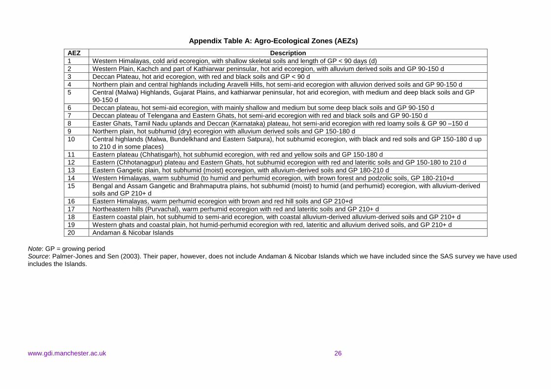
To assess locational impact, we supplemented SAS data with other data. For regional differences in

climate, state-level rainfall was averaged for 30 years (1970 to 1999).4 In addition, we controlled for

agro-ecological zones (AEZs) using the National Bureau of Soil Survey and Land Use Planning

divisions which divide the country into 20 zones based on climate, soil types, altitude, etc. (for details

see Appendix Table A). For urbanisation, we computed state-level urban to rural population using the

3 Our effective sample for analysis is slightly smaller, due to missing data on some variables for some farmers. 4 We matched information for 32 meteorological regions with the respective states.


2001 Census. State-level per capita income in the year preceding the survey (2001-02) served as an

indicator of regional variations in prosperity (GoI, 2006).5 For regional effects associated with cropping

patterns and agricultural commercialization, we divided the country broadly into three regions, each

containing several states. In principle, regional aggregation can be based on many criteria—ecology,

culture, cropping patterns, commercialisation, etc. Aggregations by culture and ecology are not

uncommon (Dyson and Moore, 1983; Agarwal, 1994, 1997). Our interest (beyond AEZs and rainfall),

however, is especially in cropping patterns and commercialisation. To capture agricultural

commercialisation, we used state-level data on marketable surplus of major food crops—rice, wheat,

maize, gram and millets (GoI 2005b; Table 1). Marketable surplus is the surplus net of the farmer’s

consumption and other needs.

Our regional categorisation for commercialization is thus as follows: Region 1 covers northwest and

west India, characterised mainly by wheat-rice cultivation and producing substantial marketable surplus

(60%). Region 2 covers the four southern states, dominated by rice cultivation and medium levels of

marketable surplus (53%). Region 3 covers central and eastern India, producing mainly rice or millets,

with limited marketable surplus (45%). We broadly term Region 1 as commercial, Region 2 as mixed

(commercial+subsistence), and Region 3 as mainly subsistence. These divisions also broadly capture

locational differences in culture and state capacity.

Table 1: Regional divisions by marketable foodgrain surplus (average for 1996-97, 1997-98 and 1998-99)

Region States within the region Marketable (marketed)a surplus as a percentage of total foodgrain production

Region 1: mainly commercial

Goa, Gujarat, Haryana, Himachal Pradesh, Jammu and Kashmir, Maharashtra, Punjab, Rajasthan, Uttar Pradesh

60.6 (60.4)

Region 2: Subsistence + commercial

Andhra Pradesh, Karnataka, Kerala, Tamil Nadu, 52.8 (53.4)

Region 3: mainly subsistence

Arunachal, Assam, Bihar, Madhya Pradesh, Manipur, Meghalalya, Mizoram, Nagaland, Orissa, Sikkim, Tripura, West Bengal

45.4 (49.4)

Source: GoI (2005b); http://agmarknet.nic.in/AbstractReportsSurplus.htm Notes: a Figures in parenthesis give the marketed surplus. All figures relate to undivided Andhra Pradesh, Bihar, Madhya Pradesh, Uttar Pradesh.

3.2. Hypotheses

Preferences can be determined by many factors and it is difficult to formalise these with precision. We

posit a set of factors that we consider relevant (based on our understanding of Indian agriculture and

the literature), and which we can test.

We conceptually club factors linked with liking or disliking farming into five types:

5 We did not use 2002-03, since 2002 was a drought year.

http://agmarknet.nic.in/AbstractReportsSurplus.htm


(i) Farmer’s endowments: access to land, irrigation, credit, and family labour (proportion of

family members in the 18-60 age group).

(ii) External support access: membership in self-help groups (SHGs), farmers’

organizations, and awareness of government support programmes.

(iii) Farmer’s personal characteristics: age, education, gender and caste

(iv) Household features: type of residence—pucca (made of brick, stone or concrete) or

katcha (made of flimsier materials).

(v) Locational characteristics (ecological and economic) where the farmer lives, such as

AEZs, and the state’s average rainfall, extent of urbanization and commercialization, and

income per capita.

We expect land owned to be linked with satisfaction in farming, but not in a linear way. Very small and

marginal farmers are more likely to dislike farming, in so far as they face more acute land constraints:

this can affect profits directly, as well as indirectly through the negative links between farm size and

access to inputs, credit (land can serve as collateral), and extension (Sarap, 1990; Dev, 2012).6 This

constraint could ease off (to an extent) as farm size increases and, with it, the proportion of those

disliking farming. Lack of irrigation is another major constraint. What matters, however, is not only

whether a farm is irrigated, but also if it has assured irrigation. Groundwater is much more reliable than

surface sources. Hence, we expect farmers with irrigation compared to those without, and those with

groundwater access versus only surface water, to be more satisfied with farming.7

Similarly, farmers with access to some credit versus none, and access to government versus mainly

private credit (predominantly moneylenders: GoI, 2005c; Subba Rao, 2006) would be more likely to like

farming. At the same time, farmers with longstanding loans would be under pressure to repay and tend

to dislike the occupation. Indeed, indebtedness causes high distress among farmers (Deshpande and

Prabhu, 2005; GoI, 2007) and is often linked with suicides (Mishra, 2006). Those connected to SHGs

and farmers’ organizations, again, would be more likely to like farming, since these can enhance

productivity and social support: SHGs provide supplementary credit, and farmers’ organisations can

increase access to input and output markets. Group membership is also linked with life or job

satisfaction (Bjørnskov, 2003; Helliwell, 2006).

Households with more adults (18-60 age group) per hectare of land operated, however, may or may

not like farming. Although family members can provide more hands for peak season operations such

as transplanting and harvesting, an excess of household adults looking for other jobs and unwilling to

do farm work can lead to overall family dissatisfaction.

On the farmer’s personal characteristics, we would expect younger respondents to be more likely to

dislike farming, since they would have aspirations beyond the world of agriculture. With few other job

6 Also, Gaurav and Mishra (2014) find that although the 1970s inverse relationship between farm size and productivity still stands for all-India, smallholders get low absolute returns and face high unit costs from purchased inputs. 7 In theory the reverse may also be possible, namely liking farming may lead farmers to buy more land or acquire better irrigation, but in practice farm land acquisition is seriously constrained in India, both in law and the land availability for sale (Rozenzweig and Wolpin, 1985). Access to irrigation is likewise constrained by external factors, especially local ecology.


options, these aspirations would remain unfulfilled. The effect of education is more difficult to predict.

Being educated can enhance farm incomes by helping the farmer gain outside contacts, information,

and bargaining power in input and output markets (see also, Panda, 2015). At the same time, education

can produce negative attitudes towards manual tasks or working in the fields. It can also raise

aspirations for white collar jobs and create dissatisfaction with a traditional occupation such as farming.8

Structural inequalities of gender and caste are also likely to matter. We would expect women farmers

to dislike farming more than men, because they face severer production constraints, and less access

to drudgery-saving equipment (World Bank, 2009; FAO, 2011; Agarwal, 2014a), apart from their double

burden of domestic and farm work. In addition, where headship overlaps with being farmers, female

household heads (who often have no adult males to help them) are likely to be especially constrained

in accessing labour and inputs. More generally, women tend to have fewer options outside agriculture

(being less educated than men, on average) and could feel more trapped in farming. Similarly,

scheduled caste (SC) or scheduled tribe (ST) farmers are more likely to be dissatisfied, since they tend

to face more production constraints (GoI, 2011).

Household characteristics can, likewise, impinge on likes and dislikes. For instance, like farm size and

education, the type of residence flags status. Hence, owning a pucca house could be linked either to

more satisfaction (since the family is doing well), or less satisfaction in that the family may have

unfulfilled aspirations beyond village life.

Finally, the farmer’s geographic location can matter. Those located in high rainfall areas are more likely

to like farming than those in semi-arid areas, since rainfall enables cultivation without irrigation at least

in the monsoon season. Similarly, favourable agro-ecological conditions could make a difference.9 In

comparison, those living in more urbanised states are more likely to dislike farming, since living near

towns or cities reveals job possibilities which contrast with the type of work farming involves. The state’s

income per capita (an indicator of overall prosperity) can again create positive feelings towards farming,

as could living in more commercialized regions (producing substantial marketable surplus and well-

connected with markets) rather than in mainly subsistence regions. As noted, these regional divisions

also broadly overlap with variations in cropping patterns, culture, and government capacity.

An equation encompassing the above variables is specified below.

8 TV Exposure to the attractions of urban lifestyles can also lead to negative attitudes towards farming among the youth. 9 Since we have 20 zones which vary by soil, climate, and altitude, we simply control for them in the regressions, rather than hypothesize the possible effect of each.


𝑃𝑟𝑜𝑏 (𝑌 = 1)

= 𝛬 (𝛼 + 𝛽1𝐿𝑎𝑛𝑑_𝑜𝑤𝑛𝑒𝑑 + 𝛽2𝐿𝑎𝑛𝑑_𝑜𝑤𝑛𝑒𝑑_𝑠𝑞𝑢𝑎𝑟𝑒 + 𝛽3𝐼𝑟𝑟𝑖𝑔𝑎𝑡𝑖𝑜𝑛_𝑠𝑒𝑎𝑠𝑜𝑛_𝑘ℎ𝑎𝑟𝑖𝑓

+ 𝛽4𝐼𝑟𝑟𝑖𝑔𝑎𝑡𝑖𝑜𝑛_𝑠𝑒𝑎𝑠𝑜𝑛_𝑟𝑎𝑏𝑖 + 𝛽5𝐼𝑟𝑟𝑖𝑔𝑎𝑡𝑖𝑜𝑛_𝑠𝑒𝑎𝑠𝑜𝑛_𝑏𝑜𝑡ℎ

+ 𝛽6𝐼𝑟𝑟𝑖𝑔𝑎𝑡𝑖𝑜𝑛_𝑠𝑜𝑢𝑟𝑐𝑒_𝑠𝑢𝑟𝑓𝑎𝑐𝑒_𝑜𝑡ℎ𝑒𝑟𝑠 + 𝛽7 𝐼𝑟𝑟𝑖𝑔𝑎𝑡𝑖𝑜𝑛_𝑠𝑜𝑢𝑟𝑐𝑒_𝑔𝑟𝑜𝑢𝑛𝑑

+ 𝛽8 𝐼𝑟𝑟𝑖𝑔𝑎𝑡𝑖𝑜𝑛_𝑠𝑜𝑢𝑟𝑐𝑒_𝑔𝑟𝑜𝑢𝑛𝑑_𝑠𝑢𝑝𝑝𝑙𝑒𝑚𝑒𝑛𝑡𝑒𝑑 + 𝛽9 𝐿𝑜𝑎𝑛_𝑔𝑜𝑣𝑡 + 𝛽10 𝐿𝑜𝑎𝑛_𝑝𝑣𝑡

+ 𝛽11 𝐿𝑜𝑎𝑛_𝑝𝑒𝑟𝑖𝑜𝑑 + 𝛽12𝐴𝑑𝑢𝑙𝑡𝑠_𝑝𝑒𝑟_𝑢𝑛𝑖𝑡_𝑎𝑟𝑒𝑎 + 𝛽13𝑆𝐻𝐺_𝑚𝑒𝑚𝑏𝑒𝑟𝑠ℎ𝑖𝑝 + 𝛿1𝐴𝑔𝑒

+ 𝛿2𝐺𝑒𝑛𝑑𝑒𝑟_𝑓𝑎𝑟𝑚𝑒𝑟 + 𝛿3𝑀𝑎𝑙𝑒_ℎ𝑒𝑎𝑑 + 𝛿4𝐹𝑒𝑚𝑎𝑙𝑒_ℎ𝑒𝑎𝑑 + 𝛿5𝑆𝐶 + 𝛿6𝑆𝑇 + 𝛿7𝑀𝑆𝑃_𝑎𝑤𝑎𝑟𝑒𝑛𝑒𝑠𝑠

+ 𝛿8𝐸𝑑𝑢𝑐𝑎𝑡𝑖𝑜𝑛_𝑏𝑒𝑙𝑜𝑤_𝑆𝑒𝑐𝑜𝑛𝑑𝑎𝑟𝑦 + 𝛿9𝐸𝑑𝑢𝑐𝑎𝑡𝑖𝑜𝑛_𝑆𝑒𝑐𝑜𝑛𝑑𝑎𝑟𝑦_𝑎𝑏𝑜𝑣𝑒) + 𝛿10𝐻𝑜𝑢𝑠𝑒_𝑡𝑦𝑝𝑒

+ 𝜃1𝑅𝑒𝑔𝑖𝑜𝑛_𝑐𝑜𝑚𝑚𝑒𝑟𝑐𝑖𝑎𝑙

+ 𝜃2𝑅𝑒𝑔𝑖𝑜𝑛_𝑚𝑖𝑥𝑒𝑑+ 𝜃3𝑈𝑟𝑏𝑎𝑛𝑖𝑧𝑎𝑡𝑖𝑜𝑛+ 𝜃4𝑅𝑎𝑖𝑛𝑓𝑎𝑙𝑙 + 𝜃5𝑠𝑡𝑎𝑡𝑒_𝑖𝑛𝑐𝑜𝑚𝑒_𝑝𝑒𝑟_𝑐𝑎𝑝𝑖𝑡𝑎

+ 𝜋1𝑀𝑎𝑖𝑛_𝑖𝑛𝑐𝑜𝑚𝑒_𝑠𝑜𝑢𝑟𝑐𝑒 + 𝜋2𝐶𝑟𝑜𝑝_𝑖𝑛𝑠𝑢𝑟𝑎𝑛𝑐𝑒 + 𝜋3𝐵𝑖𝑜𝑓𝑒𝑟𝑡𝑖𝑙𝑖𝑧𝑒𝑟_𝑎𝑤𝑎𝑟𝑒𝑛𝑒𝑠𝑠

+ ∑ 𝜆𝑗𝐴𝐸𝑍_𝑑𝑢𝑚𝑚𝑦𝑗

19

𝑗=1) … (1)

Where β, γ, δ, μ, θ, and λ respectively denote the parameter vectors for a farmer’s endowments and

resources, external support, personal characteristics, household features, location and the agro-

ecological zone. Notably, π is a vector specific to model 4 (discussed further below) which includes

variables with some missing values (and hence a smaller sample size).

4. Results

We first present results on selected characteristics of the farmers who like/dislike farming, and then the

logistic regressions which test the stated hypotheses.

4.1. Cross-tabulations

Almost all the sample farmers (99%) own some land and only 1 per cent are pure lessees. Of the

landowners, 87.4 per cent cultivate only their own land and 11.6 per cent also lease in some. Some 76

per cent of those dissatisfied with farming (relative to 61% who are satisfied) operate 1 hectare (ha) or

less (Table 2).10

Table 2: Attitudes towards farming by farm size

Farm size (operated area) Like farming Don’t like farming All farmers

(hectares) (N=30133) (N=20909) (N= 51042)

> 0.0 − ≤ 1.0 60.9 76.5 66.9

> 1.1 − ≤ 2.0 19.1 13.7 16.9

> 2.0 20.0 9.9 16.2

Total 100.0 100.0 100.0

10 One household owning 92.6 ha was omitted as an outlier; the next highest value was 60 ha .


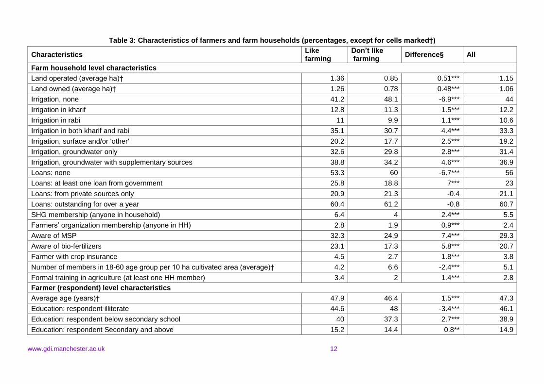
Table 3 broadly summarises the characteristics of farmers who like farming relative to those who do

not. These figures are only indicative, since the effect of a variable could change when we control for

other variables in the regressions.

We note that those who dislike farming tend to be somewhat smaller in land size. Their average

operated and owned areas are 0.85 ha and 0.78 ha respectively, compared with 1.36 ha and 1.26 ha

respectively for those who like farming. Also, among the dissatisfied farmers, a smaller percentage

have access to irrigation and credit (especially government credit), are aware of government measures

such as minimum support prices (MSPs), have crop insurance, know about bio-fertilizers, or are

members of SHGs or farmers’ organizations. In fact, across all farmers, membership in farmers’

organizations is very low (2.4%) and barely 4 per cent have ever had crop insurance. The dissatisfied

farmers, however, have more working age members per hectare—6.6 persons relative to 4.2 among

the satisfied farmers, suggesting a surplus labour situation, and have a smaller proportion with pucca

housing.

The dissatisfied farmers, relative to the satisfied ones, also tend to be somewhat younger, female, and

SC. The opposite is true for STs—unexpectedly, since STs, like SCs, have limited access to land and

other inputs, and so would be expected to be more dissatisfied. But the differences are small. Compared

to the less educated, we find a larger percentage of those educated above middle school among those

disliking farming, suggesting that the educated would prefer other jobs. Locationally, a larger proportion

of farmers are dissatisfied among those in states/regions which are less urbanized and largely in

subsistence agriculture.

Overall, therefore, the cross-tabulations suggest that the more vulnerable and resource poor farmers,

who are disadvantaged not only in their personal and household endowments but also geographic

location, are more likely to be disaffected with agriculture. The importance of each of these factors is

more robustly tested in the logistic regressions discussed further below.

4.2. Farmers’ views on why they dislike farming

What reasons do the farmers themselves give for not liking farming? Asked by the survey to select from

four possible reasons—low profitability, riskiness, low social status, and ‘other’— two-thirds opted for

low profitability and one-fifth for risk. Low profitability was more of an issue for those cultivating 1 ha or

less rather than for those cultivating over 2 ha (Table 4). Farmers in the latter category were somewhat

more likely to mention risk than profitability, but the differences across land size were not substantial.

Overall, it is thus likely that more farmers would have said they liked farming if the occupation was more

profitable and less risk-prone, or if they were less resource constrained.


Table 3: Characteristics of farmers and farm households (percentages, except for cells marked†)

Characteristics Like farming

Don’t like farming

Difference§ All

Farm household level characteristics

Land operated (average ha)† 1.36 0.85 0.51*** 1.15

Land owned (average ha)† 1.26 0.78 0.48*** 1.06

Irrigation, none 41.2 48.1 -6.9*** 44

Irrigation in kharif 12.8 11.3 1.5*** 12.2

Irrigation in rabi 11 9.9 1.1*** 10.6

Irrigation in both kharif and rabi 35.1 30.7 4.4*** 33.3

Irrigation, surface and/or 'other' 20.2 17.7 2.5*** 19.2

Irrigation, groundwater only 32.6 29.8 2.8*** 31.4

Irrigation, groundwater with supplementary sources 38.8 34.2 4.6*** 36.9

Loans: none 53.3 60 -6.7*** 56

Loans: at least one loan from government 25.8 18.8 7*** 23

Loans: from private sources only 20.9 21.3 -0.4 21.1

Loans: outstanding for over a year 60.4 61.2 -0.8 60.7

SHG membership (anyone in household) 6.4 4 2.4*** 5.5

Farmers’ organization membership (anyone in HH) 2.8 1.9 0.9*** 2.4

Aware of MSP 32.3 24.9 7.4*** 29.3

Aware of bio-fertilizers 23.1 17.3 5.8*** 20.7

Farmer with crop insurance 4.5 2.7 1.8*** 3.8

Number of members in 18-60 age group per 10 ha cultivated area (average)† 4.2 6.6 -2.4*** 5.1

Formal training in agriculture (at least one HH member) 3.4 2 1.4*** 2.8

Farmer (respondent) level characteristics

Average age (years)† 47.9 46.4 1.5*** 47.3

Education: respondent illiterate 44.6 48 -3.4*** 46.1

Education: respondent below secondary school 40 37.3 2.7*** 38.9

Education: respondent Secondary and above 15.2 14.4 0.8** 14.9


Characteristics Like farming

Don’t like farming

Difference§ All

Male farmer 73.1 71.1 2.0*** 72.3

Female farmer 26.9 28.9 -2.0*** 27.7

Farmer is male and household head 64.3 63.1 1.2** 63.8

Farmer is female and household head 5.9 7.5 -1.6*** 6.6

SC household 16.4 19 -2.6*** 17.5

ST household 16.3 14.2 2.1*** 15.4

Living in pucca house 46.4 42.3 4.1*** 44.7

Location (state-level or cross-state aggregations)

States with mainly commercial agriculture (Region 1) 37.9 35.2 2.7*** 36.8

States with mainly commercial + subsistence agriculture (Region 2) 24.1 17.6 6.5*** 21.4

States with Mainly subsistence agriculture (Region 3) 38.1 47.2 -9.1*** 41.8

State per capita income (in logs) 9.08 9.01 0.08*** 9.05

State-level urbanisation: above median value (urban to rural population ratio >0.38 ) 33.2 31.9 1.3*** 32.7

State-level: above mean rainfall (>1.35 per '000 mm) 35 38.1 -3.1*** 36.2

Notes: § Significance of difference between those liking and disliking farming, using t tests or chi-square as relevant. Significance: **at 5%; *** at 1%. HH=household


Table 4: Farmers’ reasons for not liking farming

Farm size (operated area: ha)

Reasons (per cent)

Not profitable Risky Social status Other All

> 0.0 − ≤ 1.0 67.2 17.8 5.2 9.8 100.0

> 1.0 − ≤ 2.0 65.3 22.5 6.0 6.3 100.0

> 2.0 60.4 26.8 5.0 7.9 100.0

Total 66.2 19.3 5.3 9.1 100.0

Consider now the regression analysis (Table 5 and Appendix Table B) which enables us to examine

factors beyond farmer perceptions.

4.3. Regression analysis

Table 5 presents the logistic regressions for four models (M1 to M4). M2 differs from M1 in the irrigation

variable: M1 has irrigation by season and M2, by source. M3 differs from M1 in the gender variable. In

M1 we compare male and female farmers, while in M3 we test if it matters whether the farmer is also

the household head. It needs mention that the respondent farmer was the principal person who

managed the farm and made farming decisions, and was not necessarily the household head. In

practice, 88 per cent of the males but only 24 per cent of the female farmers were also household

heads. Given the higher overlap for men than for women between household headship and being a

respondent, in M3 we substituted the dummy for the farmer’s gender with two dummies (one each for

men and women) to test the impact of being both a farmer and household head. Finally, M4 differs from

M1 in having three additional variables: main income source (farm or non-farm), crop insurance, and

awareness of bio-fertilizers. These variables were included in M4 but not the other models, since they

have some missing values. Also there could be reverse causality between liking farming and non-farm

income. M1 to M3 help us assess the effect of the variables included therein, without being affected by

a potential reverse causality effect. We also controlled for AEZs across all the models. In addition, in

our models we checked for standard errors with the cluster Primary Sampling Unit (PSU) option and

found it affected our results rather little.

We tested the presence of multicollinearity among the explanatory variables, using the Variance

Inflation Factor (VIF). The maximum VIF value was 2.9, much below 10 which is deemed

econometrically problematic (Wooldridge, 2009). Overall, the explanatory variables in the four models

correctly predict over 60 per cent of the cases.

Now consider the results.

Farm endowments and resource constraints

As hypothesized, land ownership matters a great deal, but the relationship with liking/disliking farming

is not linear. Farmers are found more likely to dislike farming if they own little land (the coefficient is

positive), but after a certain point, satisfaction tapers off (the quadratic term is negative: see also Figure

1). The predicted probability of liking farming is non-linear with respect to landownership. The peak

occurs at 18.4 ha.


Figure 1: Land ownership and the probability of liking farming

Note: The figure is based on M1 (Table 5). Predicted probabilities of a farmer liking farming were obtained for specified values of land owned, holding continuous explanatory variables at their mean.

Those dissatisfied with farming also tend to have less access to inputs, especially irrigation. As

hypothesized, farmers with irrigation in any form are more likely to like farming than those without: the

marginal effects of both seasonal and source dummies are positive and significant in all four models.

By season (M1), having irrigation in either kharif or rabi increases the likelihood of liking farming, but

(as expected) irrigation in rabi is more important, since in kharif farmers can use rainfall but in rabi they

need irrigation for a second crop or more. The impact is highest with irrigation in both seasons—the

probability of liking farming is 9.4 percentage points higher than with no irrigation—but the difference

between these farmers and those with only rabi irrigation is not statistically significant.

By irrigation sources (M2), the impact is strongest where a farmer has groundwater access

supplemented with another source. However, the insignificant difference between surface irrigation plus

‘other’ sources and groundwater alone is unexpected, since groundwater usually provides an assured

water supply which would lead to more farmer satisfaction. Possibly, some sources of groundwater,

such as wells, may be depleted.

Also, access to credit makes a significant and positive difference, but the inability to pay the loan over

time has the opposite effect. Those with access to loans—from the government or private sector—are

found more likely to like farming than those with no loans in all four models, although between

government and private credit, the difference in farmer satisfaction is not statistically significant.

However, farmers with debts outstanding for over a year are less likely to like farming.

Family labour is another potential resource. But here farmers with more working age members per

hectare are more likely to dislike farming. This suggests that the benefits of adult presence in reducing

a labour constraint is overridden by the negative effect of having adults who want to leave farming. In

particular, educated children unwilling to soil their hands with farm work could add to overall disaffection

within the family.

.5.6

.7.8

.9

Pro

bab

ility

of lik

ing fa

rmin

g

0 1 2 3 4 5 6 7 8 9 10 11 12 13 14Land owned (ha)


Table 5: Results of Logistic Regressions

Dependent variable Likes farming = 1, does not like farming = 0

Models Model 1 (M1) Model 2 (M2) Model 3 (M3) Model 4 (M4)

Explanatory variables Coeff ME Coeff ME Coeff ME Coeff ME

Land owned (ha) 0.219*** 0.051*** 0.217*** 0.051*** 0.219*** 0.051*** 0.135*** 0.031***

Land owned (square) -0.006*** -0.006*** -0.006*** -0.003***

Irrigation season dummies

(kharif only = 1) 0.136*** 0.034*** 0.134*** 0.033***

(rabi only = 1) 0.342*** 0.084*** 0.340*** 0.083***

(both kharif and rabi =1) 0.384*** 0.094*** 0.383*** 0.093***

Irrigation source dummies

(surface and/or ‘other’ sources = 1) 0.243*** 0.060*** 0.180*** 0.043***

(ground only =1) 0.329*** 0.080*** 0.229*** 0.054***

(gound with supplementary sources = 1) 0.507*** 0.122*** 0.383*** 0.088***

Loan dummies Govt (at least one loan from govt source =

1) 0.194*** 0.048*** 0.194*** 0.048*** 0.191*** 0.048*** 0.166*** 0.041***

Pvt (all loans from pvt sources =1) 0.137*** 0.034*** 0.135*** 0.034*** 0.136*** 0.034*** 0.155*** 0.037***

Loan period dummy (loan >1 yr old = 1) -0.053* -0.013* -0.054* -0.014* -0.053* -0.013* -0.025 -0.006

Household adults per 10 ha of operated area -0.003*** -0.001*** -0.003*** -0.001*** -0.003*** -0.001*** -0.002*** -0.001***

SHG membership dummy (member = 1) 0.278*** 0.068*** 0.278*** 0.068*** 0.280*** 0.069*** 0.247*** 0.058***

MSP awareness dummy (aware = 1) 0.147*** 0.037*** 0.144*** 0.036*** 0.143*** 0.036*** 0.100*** 0.024***

Crop insurance (taken =1) 0.180*** 0.043***

Bio-fertilizer awareness (aware = 1) 0.253*** 0.059***

Main income source dummy (non-farm = 1) -0.685*** -0.169***

Age of respondent (years) 0.004*** 0.001*** 0.004*** 0.001*** 0.004*** 0.001*** 0.002*** 0.001***

Respondent's education dummies

(below secondary = 1) 0.029 0.007 0.028 0.007 0.028 0.007 0.020 0.005

(secondary and above = 1) -0.099*** -0.025*** -0.099*** -0.025*** -0.094*** -0.024*** -0.062** -0.015**

Gender of farmer (male = 1) 0.082*** 0.021*** 0.085*** 0.021*** 0.040* 0.010*

Farmer is head and male 0.071*** 0.018***


Dependent variable Likes farming = 1, does not like farming = 0

Models Model 1 (M1) Model 2 (M2) Model 3 (M3) Model 4 (M4)

Explanatory variables Coeff ME Coeff ME Coeff ME Coeff ME

Farmer is head and female -0.133*** -0.033***

SC farmer dummy (SC =1) 0.006 0.001 0.002 0.001 0.005 0.001 0.061** 0.015**

ST farmer dummy (ST =1) 0.224*** 0.055*** 0.223*** 0.055*** 0.225*** 0.055*** 0.193*** 0.046***

Type of house (pucca = 1) -0.045** -0.011** -0.046** -0.011** -0.043** -0.011** -0.021 -0.005

Agriculture region dummies

Region 1 (mainly commercial = 1) 0.209*** 0.052*** 0.203*** 0.050*** 0.211*** 0.052*** 0.201*** 0.048***

Region 2 (mixed: commercial + subsistence)

0.297*** 0.073*** 0.289*** 0.071*** 0.299*** 0.073*** 0.294*** 0.069***

State income per capita (in logs) Rs. 0.162*** 0.040*** 0.156*** 0.039*** 0.164*** 0.041*** 0.135** 0.033**

Ratio of urban to rural population (state-level) -0.060** -0.015** -0.060** -0.015** -0.060** -0.015** -0.072*** -0.017***

Average rainfall (state-level) (per '000 mm) 0.351*** 0.087*** 0.355*** 0.088*** 0.351*** 0.0875*** 0.330*** 0.080***

Constant -2.432*** -2.364*** -2.448*** -1.703***

Controlled for AEZs Yes Yes Yes Yes

No of observations 50330 50330 50330 49680

Pseudo R-square 0.0467 0.0463 0.0469 0.0645

Per cent correctly classified 61.94 61.92 61.93 63.92

Notes: ME = marginal effect. Govt = government. Pvt= private. We also checked for standard errors with the cluster Primary Sampling Unit (PSU) option. Except for loan period, all other variables in our models (M1-M4) remained significant, although the level of significance in a few variables fell. Significance: *** at 1%; ** at 5%; * at 10%. Heteroscedastcity-robust standard errors have been computed. MEs were computed using the margins command in Stata/SE 13. This command gives more precise estimates of MEs in regressions involving variables specified in a quadratic form and their interactions. The significance of coefficients and MEs for variables with more than one dummy are as follows: (i) Loan source dummies: the difference between government and private sources is not significant in any model. (ii) Regional dummies: difference between regions 1 and 2 is significant in all three models. (iii) Irrigation by season: difference between kharif and rabi is significant, but that between rabi alone and 'both kharif and rabi' is not significant in model 1. (iv) Irrigation by source: difference between surface and groundwater dummies is not significant, but that between surface and ‘groundwater with supplementary sources’, and between ground and ‘groundwater with supplementary sources’ is significant in both M2 and M3.


External support access

Farmers who are aware of MSPs, belong to SHGs (and so have group support when needed),11 and

have had access to crop insurance at any time, are found more likely to like farming. Crop insurance

protects against risk of crop failure, and riskiness (as noted) is a major reason farmers gave for disliking

farming. Lack of crop insurance can leave entirely rain-dependent farmers especially vulnerable

(Gaurav, 2015). This vulnerability will increase with climate change. Awareness to MSPs helps farmers

make informed choices when selling their produce. Group membership can provide both material

support and reduce isolation when farmers face indebtedness or climatic vulnerabilities, and so reduce

rural distress. The advantages of group membership can thus go beyond the economic.

Personal and household characteristics

Age also makes a difference. Older farmers are more satisfied than younger ones. This suggests a

generational shift. It also tallies with the results for the respondent’s education. Being educated above

secondary school is linked with greater dissatisfaction. The same holds if the family owns a pucca

house. (In the cross-tabulations we had the opposite results for housing, but after controlling for other

factors pucca housing is linked with a greater likelihood of dissatisfaction.) Over time, therefore, the

young, the educated, and the better-off are most likely to want to quit farming. This resonates with

Kang’s (2010) results for Korea, where older farmers wanted to continue farming but the educated rural

youth wanted other jobs.

Female farmers, again, are found more likely to dislike farming than males (M1 and M2). It is notable

that existing gender literature on women farmers focuses primarily on their lack of resources and not

on whether they want to farm at all. Moreover, the effect of household headship is interestingly different

between men and women (M3). Male farmers who are also household heads are more likely to like

farming than those who are not. The opposite is true for women. For men, headship brings authority

and hence greater control over household resources, including family labour. For women, however,

headship is linked with certain disadvantages. Female heads are more likely to be single women

(widowed, separated) without adult male support, than women who are effectively managing the farm

while their husbands work in the non-farm sector. In the latter case, men remain household heads and

may help their wives during peak agricultural seasons. These gender dimensions pose greater

institutional challenges in making farming attractive to the farmer, compounding the earlier-discussed

production constraints and problems of accessing essential inputs and services that women farmers

face. Given that a larger proportion of men than women tend to leave farming, the associated

feminisation of agriculture could also have negative implications for farm productivity in the country,

unless women farmers are provided targeted support for overcoming their production constraints.

On caste, however, both STs (in all the models) and SCs (in M4) are found likely to be better satisfied

than other caste groups. As noted earlier, this is unexpected, since caste disadvantage tends to be

linked with production constraints. The answer may lie in what Sen (2000) terms ‘adapted preferences’,

namely that the severely disadvantaged adapt their expectations and preferences to what is feasible.

Hence they are less likely to overtly express dissatisfaction in a survey, although, as Agarwal (1994)

argues, they may do so covertly (which would not be captured in a survey).

11 In the regressions, we included SHGs but not farmers’ organizations, since the latter had missing values and very few farmers were members. Clubbing SHGs and farmers’ organizations gave very similar results to those for SHGs alone.


Locational factors

Beyond individual and household circumstances, geographic location matters. Climatic conditions

(rainfall), urbanisation, regional prosperity, and commercialisation are all significant in our results.

Farmers in high rainfall states are significantly more likely to like farming. Urbanisation has the opposite

effect. As noted, this can be interpreted in terms of the greater opportunities outside farming that urban

areas, especially large towns and cities, appear to provide, but which can create dissatisfaction if there

are no job openings, especially for the children. Other locational factors are also important. Interestingly,

farmers are most likely to like farming in regions of mixed farming—subsistence and commercial—and

least likely in largely subsistence farming areas. In terms of states, this indicates that farmers tend to

be most satisfied in the southern states and least in the central and eastern states, with the northwestern

ones coming in-between. Moreover, farmers in states with a high per capita income are found more

likely to like farming than those in poorer states.

Does access to non-farm income matter? Among existing studies, as noted, some found that non-farm

income stabilizes farm income and reduces the likelihood of farmers quitting; others found the opposite,

or got mixed results. In our reading, non-farm income is an ambiguous variable, in that those disliking

farming are also more likely to seek other occupations; hence the causation could run in the opposite

direction. Nevertheless, it is interesting to examine the relationship between the main income source

and farmer satisfaction. We find in M4 that farmers who derive their income mainly from non-farm work

are more likely to dislike farming. In other words, non-farm income does not have a stabilizing effect on

farmer satisfaction in our study.

5. Transitions beyond farming

There is a growing desire among those born into farming families to move out. Rural youth are

withdrawing from agriculture (Sharma and Bhaduri, 2007), and few farmers want their children to farm

full-time (Agarwal, 2014b). Education is seen as a way of escaping agriculture rather than as

complementary to good farming. A desire to exit, however, may not match the ability to exit.

Occupational mobility is lowest in agriculture and allied occupations: in their study based on an all-India

survey, Motiram and Singh (2010) found that almost 50 per cent of farmers’ children end up as

farmers.12

What then are the options for dissatisfied farmers who constitute such a large part of India’s work force?

Those who see smallholder farming as non-viable could argue that such farmers should move to non-

farm jobs, leaving those who like farming to continue. Such suggestions ignore several complexities.

For instance, the non-farm sector is highly heterogenous on at least two counts:

(i) Employment prospects differ between the rural and urban non-farm sectors, and in the

urban between secondary towns and mega cities.

(ii) The non-farm sector encompasses both manual, insecure, low-return jobs and highly

skilled private sector jobs, or formal government jobs.

12 Today, in some other Asian countries, the non-farm sector shows a similar occupational persistence across generations (Emran and Shilpi 2011).


Given this heterogeneity, there is no certainty that the growth of non-farm opportunities will benefit

marginal and small farmers, although they could benefit the better-educated ones (or their educated

children). Much would depend on the location and nature of employment.

Recent research on non-farm opportunities and poverty reduction is especially relevant in considering

the future of smallholders. First, at the international level, several studies covering a large number of

developing countries find that a shift from agriculture to mega cities does not reduce poverty; what

improves well-being is access to non-farm employment in the rural sector or in secondary towns, namely

in the ‘missing middle’ (Christiaensen and Todo, 2013; Imai et al., 2014). Indeed migration to mega

cities could even increase poverty (Imai et al., 2014). Moreover, when Imai et al. (2014) compare this

missing middle with the farm sector, the most poverty (and inequality) –reducing effect is through

agricultural development, and next through rural non-agricultural employment, rather than through

migration to towns or cities. And to the extent that urbanisation reduces poverty, it is mainly via rural-

urban economic linkages rather than a physical move of the rural poor to urban areas.

Second, several India-specific studies also suggest that the effect of urbanisation on rural poverty

reduction is mainly indirect, such as via increased demand for local farm produce rather than rural-

urban migration and remittances (Cali and Menon, 2013). An expanding rural non-farm sector can,

however, reduce rural poverty either directly, by increasing employment opportunities, or (more often)

indirectly through a growth in agricultural wages (Lanjouw and Murgai, 2009), or income diversification

(Krishna, 2006; Imai et al., 2015).

Third, the type of non-farm employment matters. Imai et al. (2015) find, for instance, that the main

benefits arise from access to skilled jobs (working in sales, or as clerks or professionals). Region-

specific studies also show that it is the rural high return jobs which enhance well-being and not the low

return ones accessible to the poor (Scharf and Rahut, 2014). Moreover like Imai et al.’s (2014) cross-

country results, Lanjouw and Murgai (2009) find for India that between 1983 and 2004-05 the most

important contributor to rural poverty reduction was increase in agricultural productivity (see also Datt

and Ravallion 1998 for older evidence).

This discussion raises a key question: what is happening to rural non-farm employment in India?

Himanshu et al. (2013), using NSSO data, find that although rural non-farm employment grew between

1983 and 2009-10, the growth was mainly in casual wage work, while the share of regular employment

actually declined, and in 2009-10 constituted only 20 per cent of all jobs in the non-farm sector. Not

only does regular work go to the educated, but its decline means that even among the educated only a

small percentage will find such work. Hence, although growth in rural non-farm employment may reduce

poverty it can also increase inequality (as found in Himanshu et al.’s 2013 longitudinal study of Palanpur

village).

Where does this leave the dissatisfied farmers? For the vast majority, it provides no immediate route

out of agriculture. Similarly, for the educated youth of dissatisfied farm households to leave farming

requires the growth of non-farm formal employment, or viable self-employment, and not simply casual

wage work. Hence only some will be able to quit. This returns us to the importance of raising farm

productivity for increasing the viability of smallholders.

As discussed earlier, some emphasize the potential of small farmers (World Bank, 2007; Imai et al.,

2014) while others question the evidence behind a smallholder-focused strategy. Collier and Dercon

(2014), for example, argue that large-scale poverty reduction requires a fast growth in labour


productivity, and that focusing on smallholders may not be a cost-effective route of improving the

livelihoods of poor farmers. Instead, there is a ‘good case for commercial agriculture, at a larger scale’

(Collier and Dercon, 2014, p. 98). Although Collier and Dercon focus particularly on small farmers in

Africa, their views also have many takers elsewhere, including South Asia. Imai et al. (2014), however,

argue that Collier and Dercon’s results rest on ‘shaky empirical foundations’, and instead favour

increasing agricultural productivity as the most effective poverty-reducing strategy. This would mean

supporting the smallholder. This conclusion also appears warranted in light of the difficulties of

absorbing into non-farm jobs the growing numbers of young entrants to the labour force.

A middle path could lie in policies that support smallholders as a transition strategy—one which allows

existing small farmers (an increasing proportion being women) to improve their productivity and diversify

their livelihood portfolios. Parallel to this, their children—better educated and wanting to leave farming—

could acquire the skills necessary to find regular non-farm employment somewhere in that ‘missing

middle’.

6. Concluding reflections

Unhappy farmers point to a deep malaise within Indian agriculture, which has implications not only for

the well-being of citizens and household food security but also for overall agricultural productivity. That

women tend to dislike farming more than men raises further concern, given the feminisation of

agriculture. Some might argue that given smallholder disaffection with farming the best route for them

would be to give way to large-scale farming or even corporate agriculture by a few. But this argument

ignores the fact that the most dissatisfied are also the more vulnerable, older, less educated, and

female, who cannot readily find jobs elsewhere. Our findings point to the need to help vulnerable

farmers to overcome production constraints, so that they begin to see farming as a viable profession,

or exit on their own terms rather than out of distress. Also, as noted, increasing farm productivity has

the most potential for reducing rural poverty.

To a substantial extent, reducing their production constraints would increase farmer satisfaction and

motivation, although this will not be easy, given the class and gender bias in endowments and access

to inputs and services. Many suggest a business model for agriculture through producer cooperatives

and linkages with higher value chains for enhancing the profitability and reliability of returns (including

by reducing weather-related exigencies) and so making farming more attractive, especially to the young

and educated. To some extent this is happening, but for the 80 per cent of Indian farmers cultivating

two hectares or less to adopt such models will require government support and institutional innovation

(GoI, 2011; Singh, 2014). Possible innovations could also lie in group approaches in investment and

production, including group farming, as is being tried in Kerala under its Kudumbashree Mission, and

on a lesser scale elsewhere (Agarwal, 2010; GoI, 2011). Group approaches also have global relevance,

since the majority of farmers in developing countries face an uncertain agrarian future. Indeed, some

are seeking empowerment through global movements, such as La Via Campasina. More generally,

smallholder–focused policies that seek to revive agriculture and bring about a graduated agrarian

transition could create more satisfied farmer citizens, many of whom may then decide to remain in

farming out of choice and not out of compulsion.


References

Agarwal, B. (1994). A Field of One's Own: Gender and Land Rights in South Asia (Cambridge: Cambridge

University Press).

Agarwal, B. (1997). Gender, Environment and Poverty Interlinks: Regional Variations and Temporal Shifts

in Rural India: 1971-1991, World Development, 25(1), 23-52.

Agarwal, B. (2010). Rethinking Agricultural Production Collectivities, Economic and Political Weekly,

55(9), 64-78.

Agarwal, B. (2014a). Food Security, Productivity and Gender Inequality, Handbook of Food, Politics

and Society (New York: Oxford University Press).

Agarwal, B. (2014b). Food Sovereignty, Food Security and Democratic Choice: Critical Contradictions,

Difficult Conciliations, Journal of Peasant Studies, 41(5&6), 1247-68.

Binswanger-Mkhize, H. P. (2013). The Stunted Structural Transformation of the Indian Economy:

Agriculture, Manufacturing and the Rural Non-Farm Sector, Structural Change at the State Level,

Economic and Political Weekly, 58(26 & 27), 5-13.

Birthal, P. S. Roy, D. Khan, M.T, & Negi, D. S. (2015). Farmers’ Preference For Farming: Evidence

From A Nationally Representative Farm Survey In India, The Developing Economies 53 (2):

122–34

Bjornskov, C. (2003). The Happy Few: Cross–Country Evidence on Social Capital and Life Satisfaction,

Kyklos, 56(1), 3-16.

Blanchflower, D & Oswald, A. (2004). Well-being over time in Britain and the USA, Journal of Public

Economics, 88(7-8), 1359-1386.

Borras, Jr., S.M. (2008). La Via Campesina and its Global Campaign for Agrarian Reform, Journal of

Agrarian Change, 8(2 & 3), 258–289.

Cali, M & Menon, C. (2013). Does Urbanization Affect Rural Poverty? Evidence from Indian Districts,

Policy Research Working Paper 6338, World Bank, Washington DC.

Christiaensen, L. & Todo, Y. (2013). Poverty Reduction during the Rural-Urban Transformation: The

Role of the Missing Middle, Policy Research Working Paper 6445, World Bank, Washington DC.

Clark, A. E. (2001). What Really Matters in a Job? Hedonic Measurement Using Quit Data, Labor

Economics, 8(2), 223–242.

Collier, P. & Dercon, S. (2014). African Agriculture in 50 Years: Smallholders in a Rapidly Changing

World? World Development, 63, 92-101.

Datt, G. and Ravallion, M. (1998). Farm Productivity and Rural Poverty in India, The Journal of

Development Studies, 34 (4): 62-85.

Deaton, A. (2008). Income, Health, and Well-Being around the World: Evidence from the Gallup World

Poll, Journal of Economic Perspectives, 22(2), 53-72.


Deshpande, R. S. & Prabhu, N. (2005). Farmers’ Distress: Proof Beyond Question, Economic and

Political Weekly, October 29, 4663-65.

Dev, S M. (2012). Small Farmers in India: Challenges and Opportunities, Working Paper WP-2012-014,

Indira Gandhi Institute of Development Research, Mumbai.

Dyson, T. & Moore, M. (1983). On Kinship Structure, Female Autonomy and Demographic Behaviour in

India, Population and Development Review, 9(1), 35-60

Emran, M. & Shilpi, F. (2011). Intergenerational Occupational Mobility in Rural Economy: Evidence from

Nepal and Vietnam, Journal of Human Resources, 46(2), 427-458.

FAO. (2011). The State of Food and Agriculture. FAO, Rome.

Gasson, R (1969). The choice of farming as an occupation. Sociologia Ruralis, 9(2), 146-166

Gaurav, S. (2015). Are Rainfed Households Insured? Evidence from Five Villages in Vidarbha, India,

World Development, 66, 719-36.

Gaurav, S. & Mishra, S. (2014). Farm Size and Returns to Cultivation in India: Revisiting an Old Debate,

Oxford Development Studies, http://doi.org/10.1080/13600818.2014.982081

Glauben, T., Tietje, H., & Weiss, C. (2006). Agriculture on the Move: Exploring Regional Differences in

Farm Exit Rates in Western Germany, Review of Regional Research, 26, 103-118.

Goetz, S.J. & Debertin, D. L. (2001). Why Farmers Quit: A County-level Analysis, American Journal of

Agricultural Economics, 83(4), 1010-1023.

Government of India (GoI). (2005a). Situation Assessment Survey of Farmers: Some Aspects of

Farming, NSS 59th Round, Report No. 496 (59/33/3), NSSO, Ministry of Statistics and

Programme Implementation, New Delhi.

GoI. (2005b). Abstracts of Reports on Marketable Surplus And Post-Harvest Losses of Foodgrains in

India, Directorate of Marketing and Inspection, Ministry of Agriculture, Nagpur.


GoI. (2005c). Situation Assessment Survey of Farmers: Indebtedness of Farmer Households. NSS 59th

Round, Report No. 498 (59/33/1), NSSO, Ministry of Statistics and Programme Implementation,

New Delhi.

GoI. (2006). Handbook of Statistics on the Indian Economy 2006-07, Reserve Bank of India, Mumbai.

GoI. (2007). Report of the Expert Group on Agricultural Indebtedness, Department of Economic Affairs,

Ministry of Finance, New Delhi.

GoI. (2011). Report of the Working Group on Disadvantaged Farmers, including Women, Twelfth Five

Year Plan, Planning Commission, New Delhi.

Greure, G. and Sengupta, D. (2011). Bt Cotton and Farmer Suicides in India: Reviewing the evidence,

Journal of Development Studies 47 (2): 316-337.

Helliwell, J. (2006). Well-Being, Social Capital and Public Policy: What's New? The Economic Journal,

116(510), C34-C45.



Hill, L. D. (1962). Characteristics of the Farmers Leaving Agriculture in an Iowa County, Journal of Farm

Economics, 44(2), 419-426.

Himanshu, Lanjouw, P. A., Murgai, R., & Stern. N. (2013). Non-Farm Diversification, Poverty and

Economic Mobility, and Income Equality: A Case Study in Village India, Agricultural Economics,

44,461-73.

Hye-Jung, K. (2006). Determinants of Farm Exit in Korea, Journal of Rural Development, 29(4), 33-51.

Imai, K., Gaiha, R., & Garbero, A. (2014). Poverty Reduction during the Rural-Urban Transformation:

Rural Development is still more important than Urbanisation?, BWPI Working Paper WP

204/2014, the University of Manchester.

Imai, K., Gaiha, R., & Thapa, G. (2015). Does Non-Farm Sector Employment Reduce Rural Poverty

and Vulnerability?, Journal of Asian Economics, forthcoming.

Kang, H. S. (2010). Understanding Farm Entry and Farm Exit in Korea, PhD thesis, University of

Birmingham.

Krishna, A. (2006). Pathways out of and into Poverty in 36 Villages of Andhra Pradesh, India, World

Development, 34(2), 271-88.

Lanjouw, P., & Murgai, R. (2009). Poverty Decline, Agricultural Wages, and Non-Farm Employment in

Rural India: 1983–2004, Policy Research Working Paper 4858, World Bank, Washington DC.

Martinez-Torres, M. E., & Rosset, P. M. (2010). La Via Campesina: The Birth and Evolution of Á

Transnational Social Movement, The Journal of Peasant Studies, 37(1), 149–175.

Mishra, S. (2006). Farmers’ Suicides in Maharashtra, Economic and Political Weekly, April 22, 1538-

45.

Motiram, S. & Singh, A. (2010). How Close Does the Apple Fall to the Tree? Some Evidence from India

on Intergenerational Occupational Mobility, Economic and Political Weekly, 47(40), 56-65.

Mulinge, M. & Mueller, C. W. (1998). Employee Job Satisfaction in Developing Countries: The Case of

Kenya, World Development, 26(12), 2181-2199.

Palmer-Jones, R. & Sen, K. (2003): What has Luck Got to do With it? A Regional Analysis of Poverty

and Agricultural Growth in Rural India, Journal of Development Studies, 40 (1): 1-31.

Panda. S. (2015). Farmer Education and Household Agricultural Income in Rural India, International

Journal of Social Economics, 42(6), forthcoming.

Ravallion, M. & Lokshin, M. (2002). Self-rated economic welfare in Russi', European Economic Review,

46, 1453–73.

Rosenzweig, M.R. and K.I. Wolpin (1985) Specific Experience, Household Structure, and

Intergenerational Transfers, Quarterly Journal of Economics, 100: 961-87

Sarap, K. (1990) 'Factors Affecting Small Farmers' Access to Institutional Credit in Rural Orissa, India',

Development and Change, 21, 281–307.


Scharf, M., & Rahut, D. (2014) Nonfarm Employment and Rural Welfare: Evidence from the Himalayas,

American Journal of Agricultural Economics,96(4), 1183-1197

Sen, A.K. (2000) Development as Freedom. Delhi: Oxford University Press.

Singh, S. (2014) Promoting Small Farmer Market Access in Asia: Issues, Experiences and

Mechanisms. In P. Hazell & A. Rahman (Eds), New Directions for Smallholder Agriculture (pp.

184-213). New York: Oxford University Press

Subba Rao, K.G.K. (2006). Indebtedness of Cultivator Households: Some Puzzling Results, Economic

and Political Weekly, August 12, 3460-62.

Viira, A-H, Poder, A., & Värnik, R. 2009. ‘The Factors Affecting the Motivation to Exit Farming: Evidence

from Estonia’, Food Economics: Acta Agriculturae Scandinavica C, 6, 156-172.

Wooldridge, J. M. 2009. Introductory Econometrics: A Modern Approach, 3e. South-Western Cengage

Learning.

World Bank. (2007). World Development Report 2008: Agriculture for Development. Washington DC:

World Bank.

World Bank. (2009). Gender in Agriculture Sourcebook. Vols. 1-2. Washington DC: World Bank.


Appendix Table A: Agro-Ecological Zones (AEZs)

AEZ Description

1 Western Himalayas, cold arid ecoregion, with shallow skeletal soils and length of GP < 90 days (d)

2 Western Plain, Kachch and part of Kathiarwar peninsular, hot arid ecoregion, with alluvium derived soils and GP 90-150 d

3 Deccan Plateau, hot arid ecoregion, with red and black soils and GP < 90 d

4 Northern plain and central highlands including Aravelli Hills, hot semi-arid ecoregion with alluvion derived soils and GP 90-150 d

5 Central (Malwa) Highlands, Gujarat Plains, and kathiarwar peninsular, hot arid ecoregion, with medium and deep black soils and GP 90-150 d

6 Deccan plateau, hot semi-aid ecoregion, with mainly shallow and medium but some deep black soils and GP 90-150 d

7 Deccan plateau of Telengana and Eastern Ghats, hot semi-arid ecoregion with red and black soils and GP 90-150 d

8 Easter Ghats, Tamil Nadu uplands and Deccan (Karnataka) plateau, hot semi-arid ecoregion with red loamy soils & GP 90 –150 d

9 Northern plain, hot subhumid (dry) ecoregion with alluvium derived soils and GP 150-180 d

10 Central highlands (Malwa, Bundelkhand and Eastern Satpura), hot subhumid ecoregion, with black and red soils and GP 150-180 d up to 210 d in some places)

11 Eastern plateau (Chhatisgarh), hot subhumid ecoregion, with red and yellow soils and GP 150-180 d

12 Eastern (Chhotanagpur) plateau and Eastern Ghats, hot subhumid ecoregion with red and lateritic soils and GP 150-180 to 210 d

13 Eastern Gangetic plain, hot subhumid (moist) ecoregion, with alluvium-derived soils and GP 180-210 d

14 Western Himalayas, warm subhumid (to humid and perhumid ecoregion, with brown forest and podzolic soils, GP 180-210+d

15 Bengal and Assam Gangetic and Brahmaputra plains, hot subhumid (moist) to humid (and perhumid) ecoregion, with alluvium-derived soils and GP 210+ d

16 Eastern Himalayas, warm perhumid ecoregion with brown and red hill soils and GP 210+d

17 Northeastern hills (Purvachal), warm perhumid ecoregion with red and lateritic soils and GP 210+ d

18 Eastern coastal plain, hot subhumid to semi-arid ecoregion, with coastal alluvium-derived alluvium-derived soils and GP 210+ d

19 Western ghats and coastal plain, hot humid-perhumid ecoregion with red, lateritic and alluvium derived soils, and GP 210+ d

20 Andaman & Nicobar Islands

Note: GP = growing period Source: Palmer-Jones and Sen (2003). Their paper, however, does not include Andaman & Nicobar Islands which we have included since the SAS survey we have used includes the Islands.


Appendix Table B: Summary Statistics

Definitions Descriptive statistics

N Mean SD

Farm household level characteristics

Land owned (hectares) 51412 1.06 1.84

Land owned (square) 51412 4.52 36.50

Irrigation none dummy: (no irrigation=1; otherwise=0) 51412 0.44 0.50

Irrigated in kharif dummy (yes = 1; otherwise = 0) 51412 0.12 0.33

Irrigated in rabi dummy (yes = 1; otherwise = 0) 51412 0.11 0.31

Irrigated in both seasons dummy (yes = 1; otherwise = 0) 51412 0.33 0.47

Irrigated by surface and/or ‘other’ source dummy: (yes = 1; otherwise = 0) 51412 0.19 0.39

Irrigated by ground sources only dummy (yes =1; otherwise =0) 51412 0.31 0.46

Irrigated by ground + supplementary sources dummy (yes = 1; otherwise = 0) 51412 0.05 0.23

Loan dummy, none (base category) (no loan =1; otherwise=0) 51412 0.56 0.50

Loan dummy, government (at least one loan from govt source =1; otherwise = 0) 51412 0.23 0.42

Loan dummy, private (all loans from private sources =1; otherwise = 0) 51412 0.21 0.41

Loan period dummy (loan outstanding for >1 yr = 1; otherwise = 0) 51412 0.27 0.44

SHG member dummy (any household member belongs to SHG =1; otherwise = 0) 51170 0.05 0.23

Number of adults aged 18-60 years per 10 ha operated area 51386 5.00 0.19

Main income source dummy (non-agriculture=1; if agriculture=0) 51412 0.40 0.49

Farmer (respondent) level characteristics

MSP awareness (respondent is aware of MSP =1; if not = 0) 50814 0.29 0.45

Bio-fertilizer awareness (respondent is aware =1; if not = 0) 50737 0.21 0.41

Crop insurance (farmer had crop insurance at any time =1; if not = 0) 50288 0.04 0.19

Age of respondent (years) 51412 47.28 13.53

Gender of farmer dummy (Male = 1; female = 0) 51412 0.72 0.45

Farmer is male and household head 51412 0.64 0.48

Farmer is female and household head dummy: (female and head=1; otherwise = 0) 51412 0.07 0.25

Education of respondent dummy: (illiterate = 1; otherwise = 0) 51412 0.46 0.50

Education of respondent dummy: (below secondary = 1; otherwise = 0) 51412 0.39 0.49

Education of respondent dummy: (secondary & above = 1; otherwise = 0) 51412 0.15 0.36

Scheduled Caste (SC) household dummy (SC = 1; otherwise = 0) 51412 0.18 0.38

Scheduled Tribe (ST) household dummy (ST= 1; otherwise = 0) 51412 0.15 0.36

Other caste (base) dummy (neither SC nor ST = 1; otherwise = 0) 51412 0.67 0.47

House type dummy (pucca house = 1; katcha house = 0) 51412 0.45 0.50

Location (state-level or cross-state aggregations)

Region 1 dummya (mainly commercial = 1; otherwise = 0) 51412 0.37 0.48

Region 2 dummya (mainly subsistence + commercial = 1; otherwise = 0) 51412 0.21 0.41

Region 3 dummya (mainly subsistence =1; otherwise = 0) 51412 0.42 0.49

State domestic product per capita (Rs.) in 2001-02 b (logs) 51412 9.05 0.42

State level of urbanization: ratio, urban to rural population b (2001 census) 51412 0.38 0.43

State-level average rainfall, 1970-2009 b (per '000 mm) 51357 1.35 0.65

Agro-ecological Zones (dummies)

AEZ1 51412 0.03 0.18

AEZ2 51412 0.03 0.18

AEZ3 51412 0.02 0.14

AEZ4 51412 0.06 0.23


Definitions Descriptive statistics

N Mean SD

AEZ5 51412 0.03 0.18

AEZ6 51412 0.08 0.26

AEZ7 51412 0.01 0.08

AEZ8 51412 0.06 0.24

AEZ9 51412 0.10 0.30

AEZ10 51412 0.03 0.17

AEZ11 51412 0.05 0.21

AEZ12 51412 0.06 0.24

AEZ13 51412 0.14 0.34

AEZ14 51412 0.01 0.10

AEZ15 51412 0.10 0.30

AEZ16 51412 0.02 0.14

AEZ17 51412 0.07 0.26

AEZ18 51412 0.05 0.21

AEZ19 51412 0.06 0.23

AEZ20 51412 0.01 0.07

AEZ overlap (=1 if the region falls into more than one AEZ) 51412 0.39 0.49

Notes: SD = standard deviation. MSP = Minimum support prices. govt = government. pvt = private a For states included in each region, see Table 1. b These are state-level averages applicable to all farmers in a given state.

To farm or not to farm? Indian farmers in transition - Cathie ...

Documents

Transcript of To farm or not to farm? Indian farmers in transition - Cathie ...