Mechanical design of the Magdalena Ridge Observatory Interferometer
Upload
khangminh22Category
view
1download
0
A Mobile Atom Interferometer forHigh-Precision Measurements of Local Gravity
D i s s e r t a t i o n
zur Erlangung des akademischen Grades
doctor rerum naturalium(Dr. rer. nat.)im Fach Physik
eingereicht an derMathematisch-Naturwissenschaftlichen Fakultät I
der Humboldt-Universität zu Berlin
vonDipl.-Phys. Alexander Senger
Präsident der der Humboldt-Universität zu Berlin:Prof. Dr. Jan-Hendrik Olbertz
Dekan der Mathematisch-Naturwissenschaftlichen Fakultät I:Prof. Dr. Andreas Herrmann
Gutachter:1. Prof. Achim Peters, Ph.D.2. Prof. Dr. Oliver Benson3. Prof. Dr. Markus Arndt
Tag der mündlichen Prüfung: 22.11.2011


für Sara, Ferdinand und Felix


Abstract
Precise measurements of Earth’s gravitational acceleration g areimportant for a range of fundamental problems—e. g. the Watt bal-ance as an approach for a new definition of the kilogram—and agreat tool to investigate geophysical phenomena reaching from thetopmost layers of soil to the very core of our planet. Recently, re-search efforts have been made to develop dedicated quantum sensorscapable of such measurements with very high precision and accu-racy.This thesis describes the design and implementation of such a
sensor, aiming at a superior accuracy of 0.5 ppb, resolvable in mea-surements of 24 h. A feature distinguishing this device from previouswork is its mobility, allowing for comparison with other state-of-the-art instruments, and for applications in field use in various locations.Rubidium atoms are laser-cooled and launched on a free-fall tra-
jectory. Exploiting the wave nature of quantum particles, coherentmanipulation with light pulses is used to split, reflect and recombinethe atoms’ wave-packets. The resulting matter-wave interferometeris highly susceptible to inertial forces and allows for sensitive mea-surements of accelerations.Inertial sensing with a precision of 160 nm s−2/
√Hz was demon-
strated, resulting in a measurement of g with a statistical uncer-tainty of 0.8 nm s−2 in 15 h, surpassing a conventional state-of-the-art absolute gravimeter by a factor of eight. Comparison with theGerman gravity reference net revealed a discrepancy of 260 nm s−2,well covered by the combined systematic uncertainties of 520 nm s−2.Likely causes for this deviation are identified and suitable counter-measures are proposed.
v

Zusammenfassung
Eine Reihe fundamentaler Problemstellungen setzt die genaueKenntnis der Erdbeschleunigung g voraus, z. B. die Neudefinitiondes Kilogramms im laufenden Watt-Waage-Projekt. Des Weiterensind Gravitationsmessungen ein herausragendes Werkzeug der geo-physikalischen Forschung, machen sie doch Phänomene vom oberenErdreich bis hinab in den Erdkern zugänglich. Für Absolutmessun-gen geeignete Quanten-Sensoren mit höchster Präzision sind deshalbGegenstand aktueller Entwicklungen.Diese Arbeit beschreibt die Planung und Implementierung eines
solchen Sensors, der für eine überlegene absolute Genauigkeit vonfünf Teilen in 1010, zu erreichen in Messungen von 24 h, ausgelegtist. Ein Merkmal, das dieses Instrument vor früheren Entwicklungenauszeichnet, ist seine Mobilität, die Anwendungen im Feld sowieVergleichsmessungen mit anderen Gravimetern ermöglicht.Die quantenmechanische Wellennatur von (Rubidium-) Atomen
wird genutzt, um durch kohärente Teilung, Reflexion und Wieder-vereinigung der sie konstituierenden Wellenpakete mit Hilfe vonLichtpulsen ein Materiewelleninterferometer darzustellen. Auf einEnsemble lasergekühlter Atome im freien Fall angewandt, kann de-ren Empfindlichkeit auf Inertialkräfte genutzt werden, um hochsen-sible Messungen der auftretenden Beschleunigungen zu erreichen.Eine Messpräzision von 160 nm s−2/
√Hz wird demonstriert, die
ausreicht, um g in 15 h mit einer statistischen Ungewissheit von0.8 nm s−2 zu bestimmen; dies ist um einen Faktor acht besser, alsmit den besten klassischen Absolutgravimetern üblich. Ein Vergleichmit dem Deutschen Schweregrundnetz ergibt eine Abweichung von260 nm s−2 bei einer Ungewissheit von 520 nm s−2 in den systema-tischen Einflüssen. Deren wahrscheinliche Ursachen sowie geeigneteGegenmaßnahmen werden identifiziert.
vi

Contents
1. Introduction 11.1. Gravimetry . . . . . . . . . . . . . . . . . . . . . . . . . . 8
2. Theory 132.1. Atom Interferometer in Gravity . . . . . . . . . . . . . . . 132.2. Gravity Variations . . . . . . . . . . . . . . . . . . . . . . 29
3. Experiment 333.1. Preparing the Atoms . . . . . . . . . . . . . . . . . . . . . 333.2. Interferometer Sequence . . . . . . . . . . . . . . . . . . . 423.3. Detection . . . . . . . . . . . . . . . . . . . . . . . . . . . 563.4. Vibration Isolation . . . . . . . . . . . . . . . . . . . . . . 573.5. Fountain Set-up and Mobility . . . . . . . . . . . . . . . . 663.6. Gravity of Fountain Set-up . . . . . . . . . . . . . . . . . . 703.7. Laser . . . . . . . . . . . . . . . . . . . . . . . . . . . . . . 783.8. Frequency Reference, Timing and Control . . . . . . . . . 82
4. Results 914.1. Noise . . . . . . . . . . . . . . . . . . . . . . . . . . . . . . 914.2. Gravity measurement . . . . . . . . . . . . . . . . . . . . . 98
5. Conclusion and Outlook 107
A. Details of Long-Term Gravity Measurement 111
B. Aluminium Knife-Edge Seal 115
vii


1. IntroductionMost measurements get better with a growing number of samples as statis-tics improve. The common way to reap this benefit is simply to repeat thesame measurement over and over again, paying with measurement time forincreased precision. Principal limits arise here from time varying quantitiesand from systematic drifts in the sensor. Often, the simple fact that the(life-)time of the observer is limited prohibits further development alongthis line.Another way would be to use a large set of identical sensors working
in parallel. However, this approach has rarely been used in metrology, asit is prohibitively expensive for most kinds of precision tools, and yieldsonly questionable results in case of cheap working material, which oftensuffers from uncontrollable drift and bias. Also, with a growing set of tech-nical equipment, entropy becomes a major concern, as it gets increasinglydifficult to keep everything in good working order and to obtain reliableresults.With the rapid development of matter wave optics in the past two
decades, there is a new aspect to the situation. A "new" class of ex-tremely inexpensive, ultra-stable, highly reliable and controllable sensingdevices becomes accessible, which are available essentially without limit:cold neutral atoms. For most practical purposes they pose well under-stood quantum systems with their properties given by the very nature ofour universe. In principle this enables measurements which are inherentlybound to physical constants, thus defying the need for regular calibra-tions1.In addition, there exist a large number of different elements with a wide
range of properties—and thus sensitivities to various external fields—tochoose from; the electric polarizability spanning two orders of magnitudemight serve as an example. As it has become possible to address and in-terrogate atoms with high selectivity, the full potential of quantum sensorsis beginning to unfold. And one of the many benefits is the possibility to
1It will be seen later for the instrument described here, that the measured gravityvalues are given in terms of an atomic property—a wave-vector which is related toenergy differences in electronic states—and a time span. As a frequency standardcould also be derived from the atoms, a fully self-contained measurement is possible.
1
1. Introduction
prepare large samples and to query them simultaneously with negligiblecross talk, which often allows to scale sensitivity with at least the squareroot of the number of atoms involved.While atoms themselves have been at hand for quite some time, it is the
pronounced progress in the methods necessary to prepare well defined sam-ples and to read out the effects of tiny disturbances which fuelled the rapiddevelopment of quantum sensing applications. Namely the manipulationof neutral atoms with light and the principle of matter wave interferenceare the basis for a wide range of instruments—including the one describedhere.Large scattering cross sections and the possibility to control the elec-
tronic state makes light an ideal tool to handle atoms. Moreover, lightfields can be altered rapidly and shaped with micrometer accuracy (e. g.in the form of light gratings), allowing for precise control in time and inspace. Therefore it was largely the progress in laser control2 which enabledrecent developments in the field of atom optics.With the advent of spectroscopically stabilised lasers it became feasible
to very specifically address atomic resonances, while at the same time be-ing able to provide enough intensity to induce sizeable effects. This led toa proposal by Hänsch and Schalow [1] to cool a low-density gas by illumi-nating it with intense, quasi-monochromatic light tuned to the red side of aclosed cycling transition between two electronic states. Photons scatteredby a moving atom Doppler-shifted into resonance will carry away a fractionof its kinetic energy and thus reduce its motion. Residual velocities in therange of millimetres per second are easily achievable in a few milliseconds,equivalent to temperatures of only some micro-kelvin. With this scheme—an optical molasses—first samples of laser cooled atoms were demonstratedin 1985 [2]. A substantial improvement was achieved by adding a 3D mag-netic flux gradient with vanishing flux at the point in space where thecooling beams intersect. The spatial variations in Zeeman shifts, togetherwith appropriate polarization of the laser beams, lead to net light forcesdirected to the point of zero flux. This way the atoms are confined in spacein a so called magneto-optical trap (MOT) [3].Typically 109 neutral atoms are accumulated in the volume of a pea
and can then be put on chosen trajectories, e. g. in a fountain geometry.Accelerated upwards to a few m/s, interaction times of up to a second are
2An important class of matterwave interferometer is based on mechanical gratings withtypical spacings in the range of micro- to nano-meter. The ability to prepare themin suitable qualities was developed in the same decades as for the light gratings.Often both techniques are employed in parallel.
2

well in reach while keeping the dimensions of the experimental apparatuswithin reasonable limits. This is easy enough to apply either well definedlight pulses to drive intra-atomic resonances or off-resonant light patternsacting as phase gratings. Both techniques allow for coherent manipulationof the wave-like nature of the atom.This leads to the extraordinary notion of matter waves laid down by
Louis-Victor de Broglie in his dissertation in 1924 [4]. De Broglie proposedthat there is no such thing as particles, well localized pieces of matter,but that all matter also needs to be regarded as waves, reaching into sur-rounding space, with characteristics dependent on the properties of massand velocity. This perception was the inspiration for Schrödinger’s workand thus builds one of the corner stones of quantum mechanics. It alsobrings up naturally the idea of diffraction and interference and leads tothe concept of matter wave optics, where the propagation and (self-) inter-action of particles, e. g. atoms, can be described similarly to that of lightbeams.While this started as a purely theoretical construct, soon after experi-
mental evidence of matter waves was found. First by Davisson and Ger-mer [5] and G. P. Thomson—who saw Bragg scattering of electrons incrystals—and later by Rupp [6]—who observed diffraction of electrons withman-made gratings. These experiments proved the validity of de Broglie’sideas and contributed to his Nobel prize in 1929. Ever since the objects sub-jected to diffraction have grown heavier and more complex: neutrons [7],atoms [8], simple [9, 10] and complex [11, 12] molecules with no principalobstacles hit so far.Apart from fundamental aspects, coherent manipulation of matter waves
has also proven to be a versatile tool in precision measurements. Neu-tron diffraction has evolved to a widely used technique in material andbiochemical science, and diffraction patterns in transmission electron mi-croscopy are used to study ordering of structures on molecular and atomicscales.The concept of interference was soon explored, too. First demonstrated
with electrons [13] and neutrons [14], wide adoption of this technique washindered by the involved set-ups necessary. The field of matter wave opticslacked a readily available constituent to form the analogue of light beams,and the appropriate tools to control them. It was in the rapidly devel-oping fields of cooling and manipulating neutral atoms—often with light,as mentioned above—where these shortcomings could be lifted. With ad-equate techniques appearing in the 1980s, the first atom interferometerswere presented 1991 [15–18]. Since then atom interferometer have spawned
3

1. Introduction
a broad range of scientific activity, a detailed overview of which can befound in [19].
t
zk1 k2
Path
A
Path B
π 2 π π 2
0 T 2T
state21
Figure 1.1.: Mach-Zehnder type interferometer with three light pulses. Thematter wave is split, reflected and recombined using counterpropagating pairsof lasers with wave vectors k1 and k2 at times 0, T and 2T . The atom’sinternal state is switched between |1〉 and |2〉 accordingly.
Consequently a complete interferometer can be realised with only lightto control the matter wave. An intuitive example is the Mach-Zehnder-like geometry used in this experiment, realised by three light pulses. Afterpreparation in a MOT, the cold cloud of atoms is launched on a parabolictrajectory using light forces. A first resonant light pulse chosen to switchthe electronic state of an atom with a probability of 1/2 will lead to a split-ting of the corresponding wave packet: after the pulse, the atom will be ina coherent superposition of two internal states which differ in phase andfrequency of the complementing matter wave. As the excited state carriesadditional momentum from the photons, this is associated with a bifurca-tion of the trajectory, leading to a possibly substantial spatial separation3
3In the experiment here up to 3 mm compared to the typical dimensions of atomsof < 1 nm.
4

of the two parts of the wave packet. From there on evolution of the distinctparts will lead to a growing phase shift between them, potentially furtherenhanced by the effect of additional fields due to the different susceptibilityof the atoms states.To reject the effect of time propagation and to merge the trajectories, a
second light pulse is applied at time T , shaped to switch the states withunit probability and to swap the momentum associated with the paths.This way, after 2T temporal effects in the now overlapping wave packetswill cancel, leaving only those contributions caused by external fields andthe interaction with light pulses.At this point in time a third light pulse—again with a switching probabil-
ity of 1/2—splits each part of the wave packet into the two distinct outputsof the pulse sequence. The atomic state is then the same in each individualoutput, but differs between the two. The resulting interference translatesthe unobservable accumulated phase shift into an amplitude modulationmeasurable as the ratio of the atoms in the two outputs/states. Conse-quently the sequence allows measurement of the difference in effects offields acting on the atoms, dependent on their electronic state and trajec-tory. This makes atom interferometry a highly versatile measuring toolsensitive to a range of phenomena not equally tractable by light interfer-ometers.Albeit instruments with suitable geometries to implement multi-path in-
terference were used to perform optical Ramsey spectroscopy on ultrasonicjets of metastable Helium in the late 1980s, it was realised only later byBordé, that the same set-up could be regarded as an atom interferome-ter and could be used to measure inertial forces [20]. The first dedicatedexperiments demonstrating matter wave interference with light gratingswere presented two years after this discovery and already measured accel-eration [15] and rotation [16] respectively.Since then, atom interferometry has proven to be valuable in various
fields like fundamental physics, metrology, applied physics or geophysics.It has been widely used for principal studies e. g. investigating decoher-ence [21, 22], Aharonov-Bohm and Aharonov-Casher effects [23] or Berryphase [24]. With every atom acting as an independent probe, these instru-ments are also versatile tools capable of high precision measurements—especially at microscopic scales. This enabled measurements of atomicproperties like polarizability [25], Stark shift [26, 27] and van-der-Waalsand Casimir-Polder interaction [28, 29] to unprecedented resolution. An-other remarkable result is the determination of the fine structure constantwith a fractional uncertainty of 7× 10⁻⁹ by measuring ~/matom [30, 31]—
5

1. Introduction
almost the precision offered by the best alternative method based on mea-suring the electron g-factor. A comparison of these vastly different methodsallows for checks of the underlying physics across distinct subfields withextraordinary accuracy; and substantial improvements are foreseen for thenear future.Another area where atom interferometry is expected to play an impor-
tant role is in tests of relativity. A first demonstrator to verify the weakequivalence principle was presented in 2004 [32], measuring the differentialacceleration of two isotopes of Rubidium. In the same experiment a hypo-thetical dependence on the electronic state of the atoms was also probed,which is hardly possible when relying on macroscopic test bodies. This linecan be extended even further as sufficient quantities of antimatter are be-coming available4, enabling gravitational tests on matter with very distinctquantum properties. Other proposals for equivalence tests with ordinaryatoms [35] suggest highly competitive sensitivities in the order of 10−15 andbetter. Future satellite based interferometers could also measure the grav-itomagnetic and the Lense-Thirring-effect [36] or even detect gravitationalwaves [37].Recently, it was claimed that atom interferometers of the type presented
here could also serve as a highly sensitive test for the gravitational red-shift. Re-evaluating the results of [38] former bounds of absolute mea-surements could be improved by four orders of magnitude reaching a levelbelow 10−8 [39]. These results put experiments with atom interferometersamong the most stringent laboratory tests of general relativity to date.
As massive particles are much more sensitive to inertial forces than pho-tons, applications to measure rotation, acceleration and gravitational ef-fects were amongst the first developed in the emerging field of matter waveinterferometry. As demonstrated with neutrons [42], they have been refinedwith the aid of neutral atoms to a level where they compare favourably toany other technique.Today, gyroscopes based on atom interferometry feature a precision of
6× 10⁻¹⁰ (rad/s)/√
Hz [43] and gravity gradiometers utilizing two inter-ferometers 1.4 m apart can reach 4× 10⁻⁹ s−2/
√Hz [44]. With both tech-
niques available in transportable packages, interesting applications like un-aided inertial navigation become available [45]. Furthermore, gradiome-
4A classical Moiré deflectometer with a limited precision of 1 % is proposed as a first ex-periment [33]. As interferometry with Hydrogen has already been demonstrated [34],according steps towards a similar experiment with antihydrogen seem natural.
6
year
nm s−
2Hz
103
104
105
106
107Faller
Hammond
Zumberge
Niebauer
Chu
Kasevich
Peters
1960 1970 1980 1990 2000
Typecornercubecold atoms
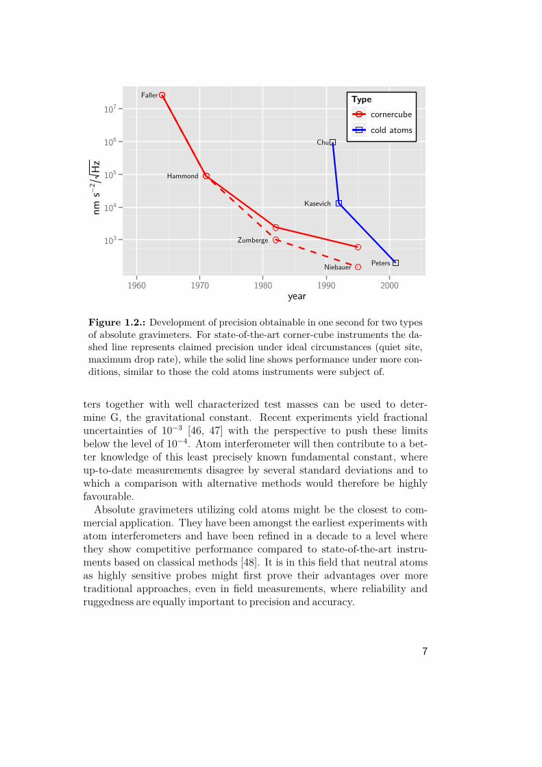
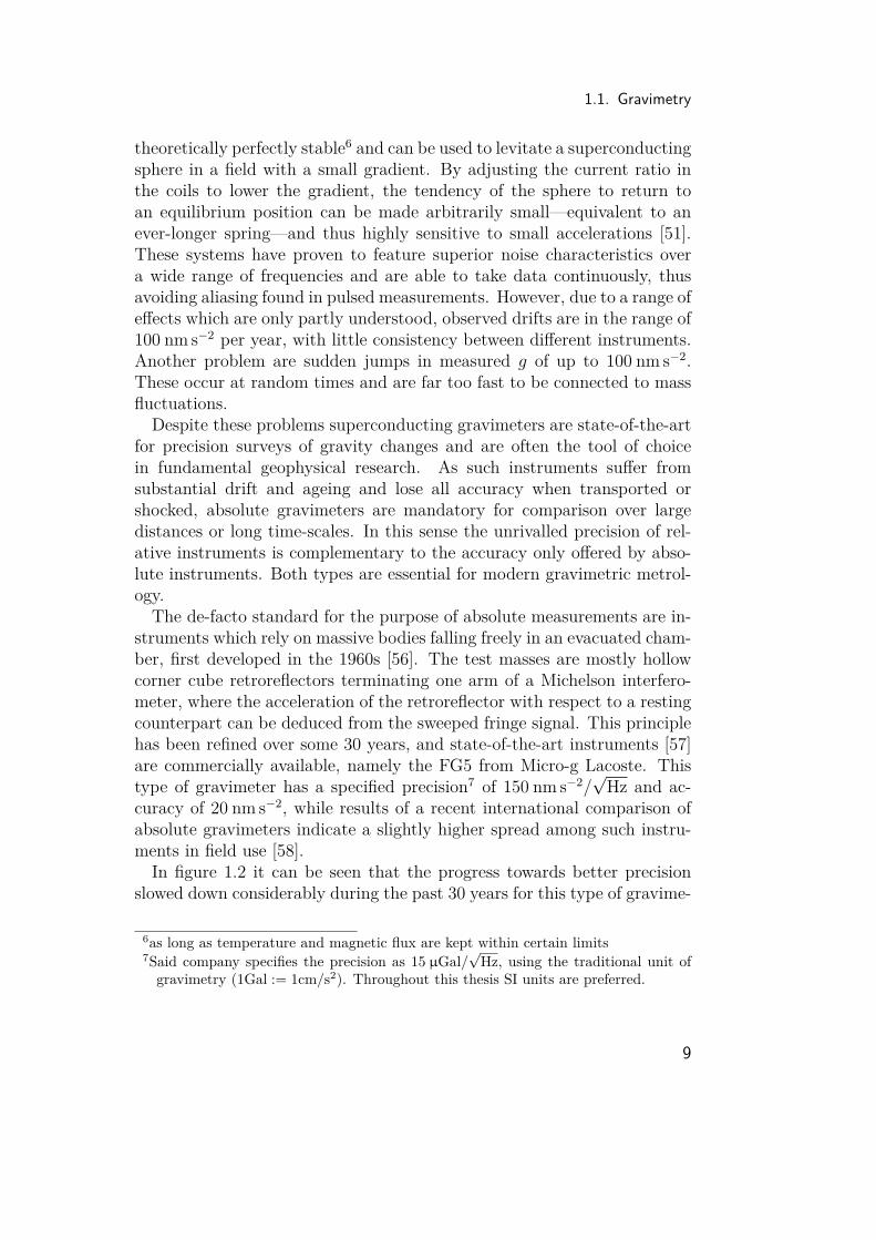
Figure 1.2.: Development of precision obtainable in one second for two typesof absolute gravimeters. For state-of-the-art corner-cube instruments the da-shed line represents claimed precision under ideal circumstances (quiet site,maximum drop rate), while the solid line shows performance under more con-ditions, similar to those the cold atoms instruments were subject of.
ters together with well characterized test masses can be used to deter-mine G, the gravitational constant. Recent experiments yield fractionaluncertainties of 10−3 [46, 47] with the perspective to push these limitsbelow the level of 10−4. Atom interferometer will then contribute to a bet-ter knowledge of this least precisely known fundamental constant, whereup-to-date measurements disagree by several standard deviations and towhich a comparison with alternative methods would therefore be highlyfavourable.Absolute gravimeters utilizing cold atoms might be the closest to com-
mercial application. They have been amongst the earliest experiments withatom interferometers and have been refined in a decade to a level wherethey show competitive performance compared to state-of-the-art instru-ments based on classical methods [48]. It is in this field that neutral atomsas highly sensitive probes might first prove their advantages over moretraditional approaches, even in field measurements, where reliability andruggedness are equally important to precision and accuracy.
7
1. Introduction
1.1. GravimetryThe precise knowledge of local acceleration due to gravity—commonly re-ferred to as g—has many virtues. It is a prerequisite for a range of metro-logical applications where some quantity is related to a force, as e. g. inthe definition of the unit of pressure or electrical current, because theforce standard is mostly realized as gravitational pull of Earth on a knownmass [49]. The Watt balance as an approach to a new definition of thekilogram—a long standing goal in the field of metrology—is a prominentexample which relies heavily on an accurate measurement of local grav-ity [50].Other applications arise naturally in the fields of geology and geophysics.
Spatial mapping of gravitational variations is besides reflection seismologythe only practical means of gathering large-volume density maps (and of-ten much less costly) and thus a standard technique of geological survey.Typical scales vary from hundreds of square kilometres e. g. in resourceexploration, up to global coverage from geostationary orbit5 in Earth ob-servation [52]. Other applications monitor long-term variations in g asin investigations of the still ongoing post-glacial rebound [53] of tectonicplates or volcano surveillance where fluctuations in the subsurface magmasystems cause alteration of local gravity [54].These measurements are often done with relative gravimeters, which of-
fer a lot of virtues. The most compact and affordable—and also the easiestto use—are instruments of the LaCoste-Romberg-type, which measure theelastic response of a spring due to variations in the acceleration of a sus-pended test-mass [55]. Their main purpose is comparison of gravity overshort distances and time-scales (tens of kilometres and hours), where withmodern devices the task of measuring is literally reduced to pushing abutton. For longer periods or travels over greater distances their limitedresolution and high drifts are forbidding, as well as their susceptibility toharsh conditions, which will introduce random shifts and variations in thescale factor. Thus frequent calibration against known gravity differences isnecessary to obtain useful results.The imperfections of mechanical springs are sought to be overcome by
use of a "perfect" spring system based on currents running in a nearly-Helmholtz pair of superconducting coils. The generated magnetic flux is
5Here it is the uni-axial gravity gradient or possibly the full tensor, which is to bemeasured. Proposed atom interferometers for this purpose share nonetheless manyof the design principals with the instrument described in this thesis.
8
1.1. Gravimetry
theoretically perfectly stable6 and can be used to levitate a superconductingsphere in a field with a small gradient. By adjusting the current ratio inthe coils to lower the gradient, the tendency of the sphere to return toan equilibrium position can be made arbitrarily small—equivalent to anever-longer spring—and thus highly sensitive to small accelerations [51].These systems have proven to feature superior noise characteristics overa wide range of frequencies and are able to take data continuously, thusavoiding aliasing found in pulsed measurements. However, due to a range ofeffects which are only partly understood, observed drifts are in the range of100 nm s−2 per year, with little consistency between different instruments.Another problem are sudden jumps in measured g of up to 100 nm s−2.These occur at random times and are far too fast to be connected to massfluctuations.Despite these problems superconducting gravimeters are state-of-the-art
for precision surveys of gravity changes and are often the tool of choicein fundamental geophysical research. As such instruments suffer fromsubstantial drift and ageing and lose all accuracy when transported orshocked, absolute gravimeters are mandatory for comparison over largedistances or long time-scales. In this sense the unrivalled precision of rel-ative instruments is complementary to the accuracy only offered by abso-lute instruments. Both types are essential for modern gravimetric metrol-ogy.The de-facto standard for the purpose of absolute measurements are in-
struments which rely on massive bodies falling freely in an evacuated cham-ber, first developed in the 1960s [56]. The test masses are mostly hollowcorner cube retroreflectors terminating one arm of a Michelson interfero-meter, where the acceleration of the retroreflector with respect to a restingcounterpart can be deduced from the sweeped fringe signal. This principlehas been refined over some 30 years, and state-of-the-art instruments [57]are commercially available, namely the FG5 from Micro-g Lacoste. Thistype of gravimeter has a specified precision7 of 150 nm s−2/
√Hz and ac-
curacy of 20 nm s−2, while results of a recent international comparison ofabsolute gravimeters indicate a slightly higher spread among such instru-ments in field use [58].In figure 1.2 it can be seen that the progress towards better precision
slowed down considerably during the past 30 years for this type of gravime-
6as long as temperature and magnetic flux are kept within certain limits7Said company specifies the precision as 15 µGal/
√Hz, using the traditional unit of
gravimetry (1Gal := 1cm/s2). Throughout this thesis SI units are preferred.
9

1. Introduction
ter. A major cause is the macroscopic dimensions of the drop mass, whichturn out to be cumbersome at very high levels of accuracy. When theretroreflector is released, the supporting floor and instrument show elasticrecoil. This leads to tilt and parasitic accelerations, which as a matter ofprinciple can not be distinguished from gravity. Furthermore, due to smalltorques imparted by the release process, the retroreflector will inevitablyrotate slowly when falling, which produces phase shifts of the reflectedbeam if the optical centre is not identical to its centre of mass [57]. Thelatter can be shifted to the former with high precision, but unavoidablewear on the drop mass will degrade the performance over time, makingregular maintenance necessary. This is why it is good practice with theFG5 to cut down the rate and number of drops to prolong maintenanceintervals, while limiting the achievable precision.The measurement principle with instruments such as the one described
here is slightly different. The idea is to very precisely pinpoint the dif-ference in falling distance, not of one, but of many test bodies betweenthree points on a ballistic trajectory. The neutral atoms employed as dropmasses offer a special benefit in this scheme. Their position at certainpoints in time—encoded as the phase of a standing laser wave—can bewritten into the phase of their quantum wave function during the opticaltransitions necessary to form the matter wave interferometer. With theoutcome of the interferometer dependent on the phase difference betweenits two paths, each atom acts thus as a separate gravity probe unencum-bered by drifts, ageing or wear. Together with the negligible effect ofreleasing only a cloud of neutral atoms8 this avoids all of the problemsnoted above. The low noise characteristics surpassing those of corner cubeinstruments by almost an order of magnitude (compare figure 1.3) allowfor a far better visibility of the remaining systematics, facilitating theircharacterisation and ultimately their control.The rapid evolution of atom gravimeters depicted in figure 1.2 gives
reason to expect that this technique will contribute substantially to im-provements in the field of geodetic metrology in the near future. It ishoped that all major systematic effects encountered so far can be under-stood, and eventually controlled, which will enable inertial measurementswith superior accuracy backed by the fundamental nature of the quan-tum sensors exploited in these systems. This is underlined by the factthat the gravimeter developed for the Watt balance project at the BureauNational de Metrologie (BNM), Paris, is based on cold atom interferome-
8approximately 10−13 g
10

1.1. Gravimetry
try [59].As can be seen in figure 1.3, g is subject to a range of influences hardly
controllable in all but some very quiet places—e. g. caves in dry, remoteareas—making it impossible to fully characterize a dedicated sensor with-out comparing it against other state-of-the-art instruments. It is there-fore highly desirable to have a set of moveable atom interferometers whichwould allow to participate in the international comparisons of absolutegravimeters organised by the Bureau International des Poids et Mesureson a regular basis9.The aim of the ongoing development is therefore to design and implement
an atom interferometer capable of absolute gravimetry with a competitiveaccuracy of 5 nm s−2. As gravimetric measurements are typically performedovernight to limit the influence of environmental noise due to traffic andother human activities, it is desirable to achieve an even better precision onsimilar time scales. Furthermore, the set-up needs to be fully mobile andcapable of rapid deployment in various locations in order to allow for directcomparison with other gravimeters and to demonstrate the outstandingpotential of quantum sensing in field applications.
1.1.1. Organization of This ThesisIn chapter two the theory to describe an atom- gravimeter with suitableprecision is summarized, and a short overview of gravitational variationsmodelling is given. A following chapter presents the experimental appa-ratus and gives some details of the measurement process. The observednoise is discussed in chapter four along with a first long-term measurement,which is compared to a determination of local gravity by a FG5 at the samesite. Finally a quick outlook on future developments follows a summary ofthe obtained results.
9Another reason is of course, that laboratories for atom physics are rarely amongst theplaces where accurate knowledge of g is most valuable.
11
1. Introduction
Resolution
SuperconductingSpring
Corner cubeCold atoms
Effectsnm
s−
2
10−1
100
101
102
103
Large scale
density var.
Tides
Volcano
activity
Human
activities
Polarmotion
Ground water
fluctuation
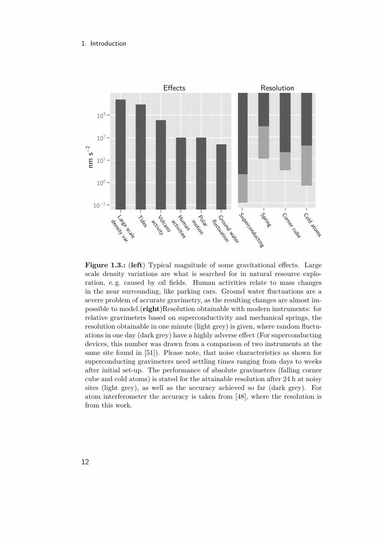
Figure 1.3.: (left) Typical magnitude of some gravitational effects. Largescale density variations are what is searched for in natural resource explo-ration, e. g. caused by oil fields. Human activities relate to mass changesin the near surrounding, like parking cars. Ground water fluctuations are asevere problem of accurate gravimetry, as the resulting changes are almost im-possible to model.(right)Resolution obtainable with modern instruments: forrelative gravimeters based on superconductivity and mechanical springs, theresolution obtainable in one minute (light grey) is given, where random fluctu-ations in one day (dark grey) have a highly adverse effect (For superconductingdevices, this number was drawn from a comparison of two instruments at thesame site found in [51]). Please note, that noise characteristics as shown forsuperconducting gravimeters need settling times ranging from days to weeksafter initial set-up. The performance of absolute gravimeters (falling cornercube and cold atoms) is stated for the attainable resolution after 24 h at noisysites (light grey), as well as the accuracy achieved so far (dark grey). Foratom interferometer the accuracy is taken from [48], where the resolution isfrom this work.
12

2. TheoryThe theoretical description of atom interferometers has been the subjectof intense studies over the past 20 years, and can be considered ma-ture in many aspects. Particularly the light-driven beamsplitter processused here [60–63] as well as appropriate interferometer geometries [64–67] are discussed in great detail elsewhere. Therefore this chapter con-fines to summarize the most important aspects, starting from very basicprinciples and adding refinements where necessary to reach the desiredprecision. A second part will bring a phenomenological overview of theprediction of gravitational fluctuations—most importantly tidal effects—as these have to be corrected for in the evaluation of experimental re-sults.
2.1. Atom Interferometer in GravityTo model the phase difference is common to split the interferometer phaseinto a part originating from free evolution and another due to interactionwith the laser beams
∆φ = ∆φfree + ∆φlight. (2.1)
This approach is valid if the beamsplitters formed by the laser pulses canbe considered thin, that is, their influence on the atoms is limited to animprinted phase-factor and a change in the atom’s momentum at a specificpoint in time. The interferometer sequence is then cut into slices of wave-packet propagation only affected by background fields where in betweenthe laser pulses are applied. The initial conditions for each piece of thepath are given by the evolution along the preceding piece adjusted by themomentum transferred by the light pulse.For a Mach-Zehnder geometry in a uniform gravitational field, the in-
terferometer takes the form depicted in figure 2.1. The formerly straightpaths are curved due to the constant acceleration in correspondence toclassical trajectories of point-like masses1. When no other external fields
1It is not a priori clear why the notion of a trajectory is appropriate for a system
13

2. Theory
are present, the situation between light pulses is not distinguishable fromthe one depicted in figure 1.1 for an observer falling freely with the atom2.According to the equivalence principle the phase difference from free evo-lution of atoms falling in a uniform gravitational field is thus the same asfor zero gravity, where ∆φfree vanishes due to the inherent symmetry of thesituation. Obviously the same holds for ∆φlight if the optics for the laserbeams would be too in free fall. It is therefore the effect of lasers fixed ina frame not influenced by the acceleration to be assessed, which enablesinertial measurements.This can be achieved by reflecting the pair of laser beams driving the
atomic transition from a mirror in rest to e. g. the centre of mass of Earth3.The phase of the light wave at any point is then given by
φlaser(z, t) = keff · z− ωeff t (2.2)
where z is the height above the mirror, keff an assigned effective wave-vector and ωeff an effective frequency. In the simplified picture the lightphase dependent on the position of the interaction is added to the wave-packets phase when the atomic state is switched during optical transitions.With the sign given by the initial state, a summation over the contributionsalong the paths curved by the constant acceleration g anti-parallel to zyields
∆φ = (φA1 − φA2 )− (φB1 − φB2 )= (keff(vrec T − 1
2 g T2) + ωeff T )− (keff(vrec T − 3
2 g T2) + ωeff T )
= keff g T2 (2.3)
with the φαi chosen as in figure 2.1 and vrec the velocity due to photonrecoil. From this equation it is evident that long T are favourable, whichare extended to 230 ms in this experiment by choosing a fountain geometry.With keff ≈ 1.6× 10⁷ this gives rise to phase shifts of about 8.6× 10⁶ rad.Given the ability to read out the phase with a precision of a few hundredmillirad a fractional single-shot precision of 10−8 in g becomes feasible.
which draws heavily from the quantum mechanical properties of its constituents. Ajustification arises from a path integral treatment, which will be discussed later.
2This is only true if the effect of the laser on any observable—e. g. the amount oftransferred momentum—does not depend on the gravitational acceleration. Forinterferometer as the one discussed here, this condition is fulfilled. However, it isnot in the case of neutron interferometers where the atoms are reflected from crystalsurfaces [42], compare [68, p. 325].
3A technically feasible approximation for this scheme is presented in section 3.4.
14
2.1. Atom Interferometer in Gravity
t
zk1 k2
Path
A
Path B
π 2 π π 2
φ1A
φ2A
φ1B
φ2B
0 T 2T
state21
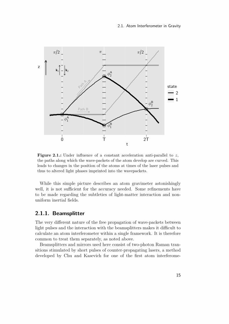
Figure 2.1.: Under influence of a constant acceleration anti-parallel to z,the paths along which the wave-packets of the atom develop are curved. Thisleads to changes in the position of the atoms at times of the laser pulses andthus to altered light phases imprinted into the wavepackets.
While this simple picture describes an atom gravimeter astonishinglywell, it is not sufficient for the accuracy needed. Some refinements haveto be made regarding the subtleties of light-matter interaction and non-uniform inertial fields.
2.1.1. BeamsplitterThe very different nature of the free propagation of wave-packets betweenlight pulses and the interaction with the beamsplitters makes it difficult tocalculate an atom interferometer within a single framework. It is thereforecommon to treat them separately, as noted above.Beamsplitters and mirrors used here consist of two-photon Raman tran-
sitions stimulated by short pulses of counter-propagating lasers, a methoddeveloped by Chu and Kasevich for one of the first atom interferome-
15
2. Theory
ters [15]. While it is possible to incorporate further light pulses into thesequence [69] or to switch to many-photon transitions (e. g. Bragg diffrac-tion) to increase the momentum transferred to the atoms and thus theresponse factor of the gravimeter, the inherent symmetry of this simplescheme facilitates control of systematic effects.
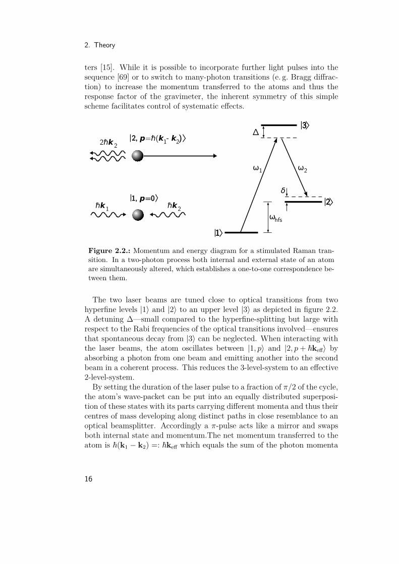
Figure 2.2.: Momentum and energy diagram for a stimulated Raman tran-sition. In a two-photon process both internal and external state of an atomare simultaneously altered, which establishes a one-to-one correspondence be-tween them.
The two laser beams are tuned close to optical transitions from twohyperfine levels |1〉 and |2〉 to an upper level |3〉 as depicted in figure 2.2.A detuning ∆—small compared to the hyperfine-splitting but large withrespect to the Rabi frequencies of the optical transitions involved—ensuresthat spontaneous decay from |3〉 can be neglected. When interacting withthe laser beams, the atom oscillates between |1, p〉 and |2, p+ ~keff〉 byabsorbing a photon from one beam and emitting another into the secondbeam in a coherent process. This reduces the 3-level-system to an effective2-level-system.By setting the duration of the laser pulse to a fraction of π/2 of the cycle,
the atom’s wave-packet can be put into an equally distributed superposi-tion of these states with its parts carrying different momenta and thus theircentres of mass developing along distinct paths in close resemblance to anoptical beamsplitter. Accordingly a π-pulse acts like a mirror and swapsboth internal state and momentum.The net momentum transferred to theatom is ~(k1 − k2) =: ~keff which equals the sum of the photon momenta
16
2.1. Atom Interferometer in Gravity
in the case of counter-propagating beams. Energy and momentum conser-vation require that the difference in frequency of the two beams satisfies
ω12 = ωhfs −~
2mk2eff (2.4)
where m is the mass of the atom.This scheme combines the advantage of metastability of the microwave
transition—enabling interferometer sequences over extended periods onlylimited by the geometry of the apparatus—with the large momentum trans-fer offered by optical photons. It is furthermore possible to very selectivelyaddress the atoms in momentum space through Doppler selection due tothe exceptionally narrow linewidth of the hyperfine splitting [68]. Thiscomes without the need of ultra-stable lasers as only the difference in laserfrequencies needs to be controlled with high precision, which is compara-tively easy.A detailed analysis of the three-level system including coupling to the
wave-packet’s momentum can be found in [60, 61]. For further discussionit is necessary to recall some of the results.As only certain impulses are allowed, it is convenient to describe the
atom in a basis of states of the form
aj,p′exp
[−i(ωAj + p′2
2m~
)t
]|j, p′〉 (2.5)
where ωAj is the energy of the jth level and the width of the wave-packet
in momentum space is negligible. The atom is subjected to a light fieldcomprising two beams
E = 12E1e
i(k1z−ω1t) + 12E2e
i(k2z−ω2t) + c.c. (2.6)
which couples to the states |1, p〉, |2, p+ ~keff〉 and |3, p+ ~k1〉 by dipoleinteraction.4Neglecting spontaneous decay from the strongly detuned upper level and
applying the Rotating Wave Approximation to the Schrödinger equation,a set of equations is obtained which govern the time evolution of the atom
4This approach neglects weak cross-coupling of e. g. |3, p+ ~k2〉 and |1, p〉 through ω2.Indeed as can be seen in figure. 3.26 some other close-by hyperfine levels of 87Rbwould need to be considered, too. However, this does not add anything profoundlynew to the situation, as all intermediate states can be eliminated adiabatically. Theinfluence of close-by transitions only needs to be taken into account, when the ACStark shift is evaluated.
17

2. Theory
during laser pulses
a1,p = i2Ω1e
i∆ta3,p+~k1 (2.7a)a2,p+~keff = i
2Ω2ei∆ta3,p+~k1 (2.7b)
a3,p+~k1 = i2
(Ω1e
−i∆ta1,p + Ω2e−i∆ta2,p+~keff
)(2.7c)
whereΩj := −e 〈j|Ej · r |3〉
2~ (2.8)
is the usual Rabi frequency.Observing that the hyperfine ground-states fluctuate much slower than
∆, the upper level can be eliminated adiabatically. After further droppingterms oscillating with ω12, a system of equations very similar to that of atwo-level-system is recovered
a1,p ≈ iΩAC1 a1,p + ieiδtΩeffa2,p+~keff (2.9a)
a2,p+~keff ≈ iΩAC2 a2,p+~keff + ie−iδtΩ∗effa1,p (2.9b)
with
ΩACj := |Ωj|2
∆ , Ωeff := Ω1Ω∗2∆
δ := (ω1 − ω2)− ω12 −p · keff
m(2.10)
Ωeff is an effective two-photon Rabi-frequency. The detuning δ is definedwith respect to a Doppler-shifted resonance without AC Stark shifts, andit is the sensitivity to this detuning which enables phase measurements inthe interferometer, as will be seen later. An influence of some importancein highly precise measurements is the weak coupling of the ground levelsto the intermediate level denoted as ΩAC
j here.It is useful to state the solution of (2.9) for a slightly detuned Raman
pulse as to identify possible systematic effects. For ωτ = π/2 + 2ε—whereω is the effective cycling frequency of the slightly detuned transition andε is a small deviation from a perfect π/2-pulse—these equations take theform [61]
a1,p(t0 + τ) = exp [i(δτ/2− ϕAC)] 1√2
((1− ε)exp [−iϕoff] a1,p(t0)
+ (1 + ε) exp[i(δt0 + π
2 )]a2,p+~keff(t0)
)(2.11a)
18

2.1. Atom Interferometer in Gravity
a2,p+~keff(t0 + τ) = exp [i(−δτ/2− ϕAC)] 1√2
((1− ε)exp [iϕoff] a2,p+~keff(t0)
+ (1 + ε) exp[i(−δt0 + π
2 )]a1,p(t0)
). (2.11b)
Accordingly a nearly perfect π-pulse of the length 2τ yields
a1,p(t0 + 2τ) = exp [i(δτ − 2ϕAC)](exp
[i(δt0 + π
2 )]a2,p+~keff(t0)
+O ((δAC − δ) + ε) a1,p(t0))
(2.12a)
a2,p+~keff(t0 + 2τ) = exp [i(−δτ − 2ϕAC)](exp
[i(−δt0 + π
2 )]a1,p(t0)
+O ((δAC − δ) + ε) a2,p+~keff(t0))
(2.12b)
where the small remnants in the original state can be neglected as they donot contribute to the output of the interferometer. Here the abbreviations
ϕAC := ΩAC1 + ΩAC
22 τ, δAC := ΩAC
2 −ΩAC1 , ϕoff ≈
δAC − δΩeff
(1+2ε) (2.13)
are used.During light interaction various phase factors are imprinted into the
atom. These need to be considered in detail. The main contribution comesfrom a detuning δ from perfect resonance of the |1〉 − |2〉-transition. If thestate is swapped, a phase shift of δ(t0 + τ/2) in case of a π/2-pulse orδ(t0 + τ) for a π-pulse is acquired with the sign dependent on the atomsinitial state. This shift can be interpreted as the phase of the perturbationat the midpoint of the pulse and justifies to treat the effect of the Ramanpulse as occurring at a specific point in time.For an atom accelerated with respect to the lasers in rest, δ is caused
by a growing Doppler shift with opposite sign for the counterpropagatingbeams and can be written as
δ(t) = vatomc
(ω1 + ω2) = (v0 − g t)keff. (2.14)
The imprinted phase is obtained as the integral over the time-dependentfrequency, which gives
φ(t0) =∫ t0
0δdt = v0t0 − 1
2gt20, (2.15)
19

2. Theory
recovering the position dependence used in the simplified picture from thebeginning of this chapter. The interferometer phase is thus the same ifassessed in a frame falling with the atoms or at rest with the lasers, ascould be expected.Related to the detuning is a factor of exp[±iδτ/2] acquired during π/2-
pulses without changing state, which is troublesome and needs to be sup-pressed, see below. Additions of π/2 during change of state ensure a phasedifference of π between both outputs of the interferometer.The phases ϕAC and ϕoff relate to combinations of the AC Stark shifts of
the ground levels. ϕAC is common to both paths of the interferometer ona per-pulse basis and therefore cancels if light intensities along the beamsare unchanged over the spatial separation of the two paths. ϕoff occurs inπ/2-pulses when conditions of perfect resonance are not met—a situationwhich is unavoidable with non-uniform intensities of Gaussian laser beamsas the AC Stark shifted frequency varies over their aperture. The effectwould only cancel if the situation was perfectly symmetric, which wouldrequire that laser intensities as much as size and position of the atomiccloud are stable over the course of the interferometer. The latter is dif-ficult to achieve due to finite velocities of the laser cooled atoms, whichgives raise to a significant systematic in a high precision atom interferome-ter [48]. The effect can be suppressed by choosing a ratio of laser intensitieswhere the AC Stark shifts of both ground levels become the same and theirdifference—which leads to ϕoff—therefore cancels. This is possible even ifvarious cross-couplings are taken into account, as each separate shift causedby a particular coupling is dependent on the detuning of the correspond-ing laser frequency from the addressed optical transition; see also [70] fora detailed calculation.
2.1.2. Thick BeamsplittersThe analysis outlined above is helpful to understand some characteristics oflight-matter interaction and to identify a harmful systematic effect. But itis sufficient only if the effect of the beamsplitters on the wave-packet’s shapeand trajectory can be neglected. With the high precision obtainable in aninstrument like the one described here, such modifications have to be takeninto consideration, especially when evolution of the atom is influenced byadditional gravito-inertial fields.When a laser pulse is applied, the atom propagates through a periodic
potential similar to a "light crystal". As in e. g. diffraction of neutronsin highly ordered materials, this results in an altered dispersion relation
20

2.1. Atom Interferometer in Gravity
for those waves allowed to travel in the crystal. For an (effective) two-level system an analytical treatment is given in [62], yielding the condition(
(p + ~keff)2
2m − E ′ − ~∆)(
p2
2m − E′)− ~2Ω2
eff = 0 (2.16)
with E ′ = E− 12(E1 +E2)− ~
2∆, E the total energy and E1,2 the energies ofthe ground states. For a given E ′ this fourth-order equation allows for fourmomenta, that is p1,2 and p1,2 + ~keff, where for the z-component pz1 = pz2due to the symmetry of the situation.Propagation of the wave-packet is governed by its group velocity υ, which
is not necessarily proportional to the momentum due to the modified dis-persion relation. Instead
υ = ∇pE′ (2.17)
which for the interesting z-component gives
υz1,2 = pz
m+ 1
2
(1± y√
1 + y2
)~keffm
, (2.18)
wherey := 1
2~Ωeff
((p + ~keff)2 − p2
2m − ~∆)
(2.19)
vanishes in case of perfect resonance. This is an interesting result as itstates that if y = 0 the wave-packet does split only after the light pulse.Before both parts evolve along the same curve, which is given by the meanof the unperturbed path and that carrying the additional momentum fromthe two photons. Deviation from the resonance condition will result infour distinct parts, where two pairs differ in the photon momentum carriedand the constituents of each pair in the momentum perpendicular to thebeam. Such cases would complicate the interpretation of experimentalresults considerably.As covered in [71] gravitational acceleration during the beamsplitter
process leads to such a detuning and consequently to significant changesto the beamsplitter-process. This is why it is good practice in atomgravimeters to compensate the growing Doppler shift by adequately tuning("chirping") the laser frequencies. The information otherwise read fromthe phase difference between the two paths is thus shifted into the ratewith which the frequency needs to be chirped in order to retain resonance,indicated by all atoms being in the initial state in the interferometer out-put.
21

2. Theory
t
z
τ
T2τ
Tτ
t1 t2 t3
state21
Figure 2.3.: Trajectories due to modified propagation during light pulses.The limit of infinitely thin beamsplitters (light grey, straight) is to becompared to the situation where both paths feature the same group velocityin the "light crystal"(black). To obtain a comparable picture with gravity(light grey, bent) the laser frequencies have to be chirped in order to retainresonance.
The change in group velocity during light interaction implies a spa-tial shift and consequently corrections to the phase acquired in successivebeamsplitters even for the "unperturbed" path. This also slightly affectsthe dependence of the interferometer on g, making a re-evaluation neces-sary.Full analytic treatment of the atoms subjected to strong electro-magnetic
interaction is only possible for certain spatial or temporal geometries of thelight fields. For a rectangular profile in the time domain (square pulses)the details have been worked out in [72] with a discussion of the case ofinterest here: a three-pulse interferometer with the spatio-temporal Mach-Zehnder geometry from above and pulse durations of τ and 2τ respectively,separated by periods of free evolution of length T .The result is that if the width of the initial wave-packet in momentum
22

2.1. Atom Interferometer in Gravity
space is smaller5 thanmΩeff/keff, further dispersive effects of the beamsplit-ter can be neglected. Due to the altered trajectories in the beamsplittersof finite length, the interferometer geometry then resembles figure 2.3 andthe overall phase shift6 becomes
∆φlight = keff · gT (T + 2τ) + ϕbsp (2.20)
where the modified time dependence can be attributed to the adjustedspatio-temporal area enclosed be the two interferometer arms. An addi-tional phase ϕbsp of the order O(T τ) is to be added, if the condition y = 0is not met at all times.It is further worth noting, that the action of the beamsplitter can still be
reduced to an instantaneous effect at a specific point in time (generalizedttt scheme [72]), while the atom is otherwise considered to evolve underinfluence of the external fields only, albeit on perturbed trajectories. Thisis the justification for a separate treatment of light fields and free evolution,even in the case of strong laser fields.
2.1.3. Free EvolutionWhile the biggest part of the phase shift accumulated in the interferometersequence is due to light interaction, understanding the effect of externalfields acting on the atoms is crucial to make highly accurate measurements.Especially non-uniform inertial fields need to be taken into account, asthese shift the energy of the two arms of the interferometer differently,which possibly leads to a significant phase offset.Calculating the propagation of the wave-packets by solving the Schrö-
dinger equation over full periods between light-interaction would be cum-bersome, especially when variable fields are involved. A treatment in theposition picture is then appropriate, where the advantage of the momen-tum picture—each component can be treated separately in a closed familywith a finite number of states—is lost.The situation is alleviated considerably if the action
SΓ =∫ tb
tadtL[z(t), z(t)] (2.21)
along the possible paths Γ an atom can take is much larger than ~, that is in5This can be ensured by selecting a narrow velocity class of atoms, see the next chapter.6This holds in the limit of very small detuning, that is very small gravity or adequatelychirped lasers.
23
2. Theory
the classical limit of macroscopic paths. This results in the phase SΓ/~ of amatter wave assumed to follow Γ to be a highly oscillatory function of evenmicroscopic path variations, as long as it is not the path which makes SΓstationary. In such case only the neighbourhood of the distinguished pathΓcl will add significantly when contributions of all possible paths startingfrom a certain point za := z(ta) are allowed to interfere in a chosen endpointzb := z(tb). According to the principle of stationary action Γcl is the patha classical particle would travel along and, with the reasoning just given,also the path which determines the phase of a quantum particle in theclassical limit.This limit defines the picture in which a description of an atom inter-
ferometer as in figure 1.1 makes sense. The depicted paths are those thecentres of mass of the atom’s wavepacket fragments can be thought of topropagate on. This is not exactly true as the contributions of all possiblevariations of the path need to be summed at the endpoint, but those notvery close to the classical path do vanish due to destructive interference.As detailed in e. g. [73], if additionally the Lagrangian of the system is atmost quadratic in coordinates and momentum, the Feynmann path inte-gral can be separated so that the phase of the quantum particle at zb isonly given by its initial phase and the—now classical—path integral alongΓcl.Applying this principle to the problem of free evolution greatly simplifies
the calculation. For the phase in the interferometer this gives
∆φfree = 1~
∮ΓclLdt (2.22)
where Γcl is the closed loop formed by path A and B concatenated together.If unknown, the precise trajectories can be derived from e. g. the Euler-Lagrange equation.In the case of uniform acceleration g the Lagrangian reads
L = m
2 z2 −mgz (2.23)
which needs to be integrated along sections of the well-known form
z(t) = za + za(t− ta)− 12g (t− ta)2, (2.24)
where za := z(ta).The interferometer loop consists of four sections (first/second half, up-
per/lower path) where initial velocities differ by vrec = ±~keffm
between
24
2.1. Atom Interferometer in Gravity
concurrent sections. Obeying the orientation of the path during integra-tion yields indeed vanishing action after some straight-forward calcula-tions.
2.1.4. Gravity GradientOn Earth’s surface a scalar gravity gradient of about γ = 3× 10³ nm s−2/mis present, leading to a significant difference in acceleration of approxi-mately 750 nm s−2 over the height of a typical interferometer sequence and10 nm s−2 over the spatial separation of the paths.The Lagrangian now takes the form
L = m
2 z2 −mgz + m
2 γz2 (2.25)
from which the classical path can be derived by evaluating the Euler-Lagrange equation, giving
z(t) = g0
γ+(z0 −
g0
γ
)cosh(t√γ) + v0√
γsinh(t√γ) (2.26a)
z(t) =(z0 −
g0
γ
)√γ sinh(t√γ) + v0 cosh(t√γ). (2.26b)
The hyperbolic trajectories resulting from the small linear component ontop of the constant background lead to some deviations from the situationfrom before, most notably a small gap ∆z in the endpoints of the twopaths of a few Å. This is not harmful as the width of the wavepacket is atleast 4 µm7, ensuring almost unaffected overlap. A small difference in theend-velocities of ≈ 2× 10⁻² nm/s gives rise to a very slow beat of the twowavepackets in each output. With time spans of about 150 ms between thelast Raman pulse and detection and a mean velocity of roughly 2 m/s theresulting phase offset of ≈ 1 µrad is negligible.The lengthy calculation of the phase from the action along the hyper-
bolic paths is best done using computer algebra. When adding a smallcontribution p∆z/~ from a non-classical path segment to bridge the gapbetween end-points [73], the obtained result is
∆φgrad, free = keff
(vrec2√γ (sinh(2T√γ)− 2 sinh(T√γ))
), (2.27)
7Estimated from the uncertainty in the initial momentum after velocity selection, seenext chapter for experimental details.
25

2. Theory
which amounts to 3 mrad or 4 nm s−2 for typical T = 230 ms and gradi-ents as given above, and becomes important for highly accurate measure-ments.However, the effect on the contribution from laser phase is much larger.
Calculating the phase from the position of the atoms at times of the Ramanpulses8 yields
∆φgrad, light = 4γ
sinh2(T√γ
2
)((γz0 − g0) cosh(T√γ) +√γv0 sinh(T√γ)) ,
(2.28)which leads to a shift of −0.520 rad or −610 nm s−2 under typical experi-mental conditions, where v0 = 2.2 m/s and z0 = 0 is the choosen height ofthe first pulse.If expanded in γ to first order, measured gravity due to the laser phase
is written as
ggrad, light = g0 − γ(z0 +
(v0 + ~keff
2m
)T − 7
12g0T2)
+O(γ2). (2.29)
From the expression in brackets a gradient-dependent height-correction canbe drawn, specifying the point at which the actual value of g equals themeasured one. This is at 1.35 m—close to the apex—for a height of thefirst pulse of 1.15 m. It is also evident that in order to determine g with anaccuracy of 5 nm s−2, the height of the interferometer needs to be knownwith an uncertainty of ≈ 1 mm.
2.1.5. Transfer Function of the InterferometerTo ease characterization of the instrument, it is useful to be able to calcu-late the impact of observed perturbations on the outcome of the interfero-meter. A convenient method is the sensitivity function, which gives therelation between small phase fluctuations δφ occurring at random timesin the Raman beams and the resulting shift ∆φ(δφ, t) deduced from theratio of atoms. In a further step the transfer function can be derived fromthe Fourier transform of the sensitivity function, which is helpful to assesse. g. the variance in measured values of g resulting from a given spectraldistribution of noise densities.
8Exactly the same results for the contributions of free evolution and laser interactionare obtained by Bordé in [65], using a framework which is the quantum-mechanicalequivalent to the ABCD-matrices known from geometrical optics.
26

2.1. Atom Interferometer in Gravity
The sensitivity function is defined as
g(t) := limδφ→0
∆φ(δφ, t)δφ
(2.30)
which for an atom interferometer measuring at the slope of the fringe canintuitively be evaluated being -1 for the first half of the interferometersequence, +1 for the second and zero otherwise, as either the middle orthe last Raman pulse write the resulting phase into the atoms. A smallmodification is necessary due to the finite width of the pulses, which iscalculated in [74] to be
g(t) =
sin (Ωeff(t+ T )) −T − 2τ ≥ t > −T − τ−1 −T − τ ≥ t > −τ
sin (Ωefft) −τ ≥ t > τ1 τ ≥ t > T + τ
− sin (Ωeff(t− T )) T + τ ≥ t > T + 2τ0 else
(2.31)
where for convenience t = 0 coincides with the middle of the π-pulse. TheFourier transform [74]
G(ω) : =∫ ∞−∞
e−iωtg(t)dt (2.32)
= 4iΩeff
ω2 − Ω2eff
sin(ω(T + 2τ)
2
)(cos
(ω(T + 2τ)
2
)+ Ωeff
ω
(ωT
2
))
can be used to examine fluctuations in the frequency domain. To this endone observes that (2.30) is equivalent to
∆φ =∫ ∞−∞
g(t)dφ =∫ ∞−∞
g(t)dφdtdt. (2.33)
Making use of the Plancherel theorem, this leads to
Var(∆φ) =∫ ∞−∞|H(ω)|2 Sφ(ω)dω (2.34)
where Sφ(ω) is the power spectral density of the phase fluctuations and Hthe transfer function given by
H(ω) := ωG(ω). (2.35)
27
2. Theory
For the last definition it is used that with h = eiωt∣∣∣F(h)∣∣∣2 = ω2 |F(h)|2 (2.36)
for any real-valued ω 6= 0.Vibrational noise is often the biggest concern in the gravimeter. It ex-
presses itself as phase fluctuations caused by movements of the mirror re-flecting the pair of Raman beams9, which can be quantified as
δφ = k1 · δz− k2 · δz = keffδz. (2.37)
Vibrations are easily measured as residual accelerations with suitable seis-mometers, which is why the transfer function is often needed for δa = δz.Using (2.36) again gives
Ha(ω) = keffωG(w). (2.38)
As can be seen from figure 2.4, the interferometer exhibits a strongly mod-ulated sensitivity to fluctuations when examined in the frequency domainwith overall characteristics of a bandpass and a lowpass respectively. Thisis due to accumulation of said fluctuations in between and averaging dur-ing beamsplitters, limiting the susceptibility to certain ranges of frequen-cies.The considerations from above do not account for the cyclic character of
the interferometer. To cover extended periods in time, the interferometersequence needs to be repeated with a (fixed) repetition rate. As everysampled system with a duty cycle less than unity, it thus becomes proneto aliased signals present at frequencies which are an integral multiple ofthe repetition frequency. However, this behaviour depends strongly on thecoherence time of the noise signals, making e. g. high-frequency oscillationsin electronic control loops particular cumbersome. Here the assumption ofuncorrelated noise was made, where each measurement is independent frompreceding cycles.
9Vibrations are far less critical for all other optical elements, as they affect both beamsequally, so that the resulting deviations in phase cancel in the interferometer.
28

2.2. Gravity Variations
Frequency [Hz]
Norm
alize
d Sq
uare
d M
odul
us
10−710−610−510−410−310−210−1100
10−710−610−510−410−310−210−1100
10−2 10−1 100 101 102 103 104 105
phaseacceleration
Figure 2.4.: Normalized transfer functions of phase and acceleration. Forthe calculation T = 230 ms and τ = 20 µs. For frequencies higher than 150 Hzonly the mean is depicted.
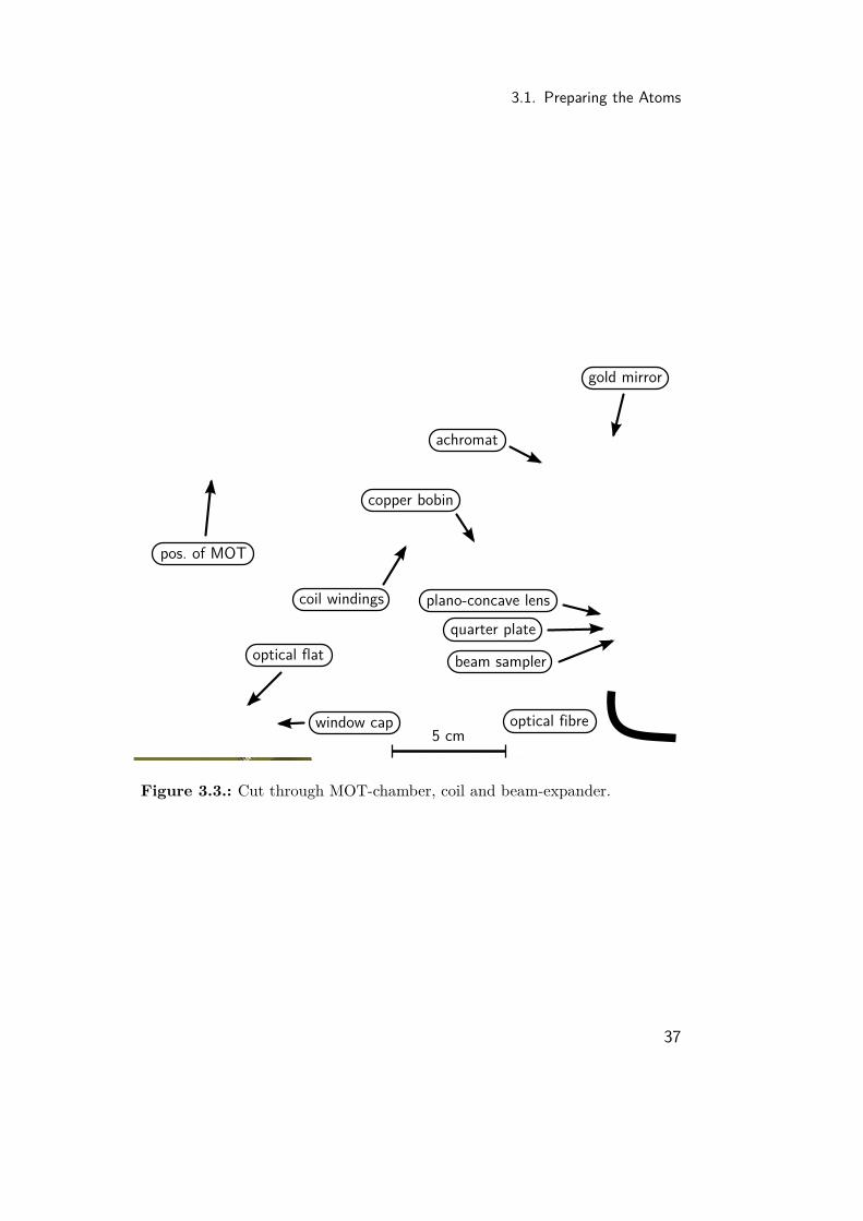
2.2. Gravity VariationsA challenge associated with highly accurate determinations of local gravityis its pronounced variability in time and space, which can amount to up to2000 nm s−2 during typical measurements. Often these variations are notthe object of interest, but rather perturbations to be rejected to obtain thetargeted accuracy of a few nm s−2. The situation is further complicated bymany of the disturbing sources not being fully understood or random andtherefore hard to predict. Luckily these disturbances are often either ofhigh frequency (vibrations), rare (e. g. rapid change of ground water leveldue to massive rain fall) or very slow (e. g. postglacial rebound of the crust,a few 10 nm s−2 per year) and can be filtered out.An influence which needs modelling to be removed is the time-dependent
gravitational effect of celestial bodies, especially Sun and Moon, and theelastic and inelastic answer of Earth’s masses. While the former couldbe calculated rather straightforward from ephemerides, the latter is only
29

2. Theory
partly understood and subject of research which reaches back to the 18thcentury. Modern models include effects of a rotating ellipsoidal earthwith elastic core, liquid outer core, inelastic mantle and some hydrody-namical aspects of mantle convection [75] complemented by the effectsof large water masses (oceans and seas), their redistribution and reso-nant excitation as well as elastic reactions of the crust to their load-ing [76].To connect these models with observations and to give predictions in
a consistent manner, an agreed mode of description is needed. This iscommonly done in the frequency domain. In time the most important con-tributions are of periods of half and full a day due to Earth’s rotation, withthousands of frequencies needed if one wishes to account for the subtle in-fluence of all planets in our system [77]. Still, most of the effect (> 99 %) iscontained in a dozen spectral components related the dynamics of the sunand the moon [78]. To characterize a site from measurements or to commu-nicate a prediction, amplitude- and phase-factors for each component aregiven, as in appendix A for the physics department of the Humbold Uni-versität zu Berlin. Here, the major part is from solid earth (> 90 %), withthe rest caused primarily by oceanic tides (up to 10 % close to coasts, drop-ping to a few percent inside continents). The remaining deviation found inmeasurements needs other explanations, see below.In the space domain it has proven useful to develop Earth’s gravity
potentialV⊕ = G
∫∫∫ dm
s(2.39)
with G the Gravitational constant and s the distance of a point outsideEarth’s ellipsoid to the infinitesimal mass dm into a series of sphericalharmonics Ylm
V⊕ = GM
r
(1 +
∞∑l=1
l∑m=0
(a
r
)lClmYlm
). (2.40)
Here M is Earth’s mass as the coefficient of the spherical harmonic ofdegree 0, a the major axis of the ellipsoid and r the distance to Earth’scentre. This series converges rapidly and can be truncated at any degree land order m when sufficient spatial resolution is reached. Modern approxi-mations from large scale satellite measurements can go up to l = m = 200,equivalent to spatial resolutions of 100 km [79], and are patched with localgravimetry when higher resolution is needed. To assess the gravitationalmodulation the (time-varying) gravity potential of celestial bodies can also
30

2.2. Gravity Variations
be developed around earth as such a series [80]. From these, predictions canbe derived with the help of the models from above.Sensitive measurements with a resolution of 100 nm and below also need
correction for polar motion, variations in Earth’s rotational frequency andlocal weather. Polar motion—the slow movement of Earth’s rotationalaxis with respect to its body—and length of day changes modulate the lat-itude dependent centrifugal acceleration and are easily corrected for whenknown, e. g. from the International Earth Rotation and Reference SystemsService [81].The impact of atmospheric fluctuations is much harder to predict. It
can be split into gravitational pull and elastic loading of the crust lead-ing to height changes, which both modulate with barometric pressure. Tobe modelled correctly, information about local air distribution as well aslocal geology is necessary [82], making exact predictions tedious. There-fore for standard gravimetric measurements these effects are most oftenestimated by a simple linear factor of 3 nm s−2/hPa and referenced to thesite-dependent standard pressure
pn = 1013.25(
1− 0.0065h288.15
)5.2559
[hPa] (2.41)
with h the topographic elevation.To ease the calculations in strive for a prediction of local gravity changes,
several programs are available. One is TSoft, developed by the RoyalObservatory of Belgium [83], which can compute synthetic tides of solidearth natively and the effects of polar motion and ocean loading when givenappropriate parameter sets. A comprehensive source for ocean loadingcoefficients calculated for a given site is [84]. A typical dataset obtainedfrom such computations is shown in figure 2.5 and later used for correctionsof a first long-term measurement, see section 4.2.
31

2. Theory
date in 2010
nms2
−1000
−500
0
500
−10−5
05
1015
23.5
24.0
24.5
25.0
29.Nov 6.Dez
solid earthocean loading
polar motion
Figure 2.5.: Predicted tides including solid earth, ocean loading and polarmotion effects for a location close to the physics department of HU-Berlin.The typical modulation due to Sun and Moon is apparent.
32
3. ExperimentTo obtain high precision measurements with the atom interferometer, somecare has to be taken when preparing and launching the atoms. First, a suit-ably high number of atoms has to be collected and cooled to sub-Dopplertemperatures, which is done in a MOT with adjacent optical molasses.The cloud of cold atoms is then launched upwards with the help of lightforces and subjected to a series of selection processes in order to obtain apure sample with low momentum spread in a magnetic insensitive internalstate. This sample is processed in the actual interferometer sequence ina zone well shielded from external influences close to the apex of its freeflight parabola. On its way down, the two outputs of the interferometerare interrogated by detection of resonantly scattered light, from which theratio of atoms in the outputs and thus the phase shift between the twoarms of the interferometer can be deduced. This procedure—from here onreferred to as a "shot"—takes a bit more than a second, and is repeated inan endless loop to obtain a time series of gravitational data. In the follow-ing sections a more detailed walk through the apparatus and the necessarysteps is given.Due to the absolute nature of the measurements to be taken, systematic
effects are of highest importance and have been examined thoroughly inprevious work [61, 85–87]. Still there are areas found, where the publishedresults lack the details necessary to cover all thinkable aspects of erroneouseffects. While not yet studied in greater detail, some considerations topossible influences are added, when appropriate.
3.1. Preparing the AtomsThe choice of 87Rb as the atomic species for the interferometer is motivatedmostly by its first optical resonances being in the near infrared, which canbe addressed conveniently by diode lasers. These devices and suitable lightamplifiers based on the same semiconductor technology allow for small,rigid and comparably cheap light sources for the optical system; qualitiesmost valuable in transportable devices. The D2-resonance offers further-more a strong cycling transition from 52S1/2,F = 2 to 52P3/2,F′ = 3 with
33

3. Experiment
vibration isolated mirror
state selection
MOT and velocity selection
detection
π/2-pulse
π/2-pulse
π-pulse
Raman beams
µ-wave
laser light
Figure 3.1.: Steps in a measurement cycle and their corresponding positionsin the fountain apparatus. For clarity the flight parabola has been spreadsidewards; in reality the atoms are launched exactly vertical.
34
3.1. Preparing the Atoms
only a small escape probability along the F′ = 2 hyperfine level, which sug-gests a scheme for the laser frequencies as depicted in figure 3.26.
3.1.1. MOT and Optical MolassesThe cold Rb-atoms are prepared in a MOT in 1-1-1-configuration [88] fromlow density thermal background. The Rb-vapour is provided by means ofresistively heated dispensers manufactured by SAES getters. They allowfor fine grained control over vapour pressure by adjusting the heating cur-rent and release a natural isotope mixture containing approximately 27 %of 87Rb with low contamination by other substances. The yield of a pairof standard dispensers was found to be sufficient for more than 1500 h ofcontinuous operation.The cooling beams feature a 1/e2 diameter of 30 mm and 20 mW of laser
power per beam. From 10−9 hPa of Rb vapour close to 109 atoms areaccumulated in 595 ms into a roughly spherical cloud of about 5 mm indiameter.After switching off the Anti-Helmholtz-coils and an additional eddy cur-
rent decay time of 5 ms an optical molasses with growing red-detuningof up to 20Γ (Γ being the natural line width) of the cooling beams fol-lows. The far-detuned phase is ended after 3 ms by adiabatically cuttingoff the cooling light and retaining the repumper for another millisecond,in order to have all atoms in the F = 2 hyperfine ground state. Whenmagnetic background fields are carefully compensated for with the helpof three perpendicular pairs of Helmholtz coils fixed around the MOTassembly, this procedure gives a temperature deduced from the velocityspread of the atoms of 6 µK, limited by short term fluctuations. Thesewere found to correlate strongly with variations of the background mag-netic flux, probably caused by technical equipment in the laboratory. Itseems likely that lower temperatures can be achieved when their influenceis removed through suitable shielding.During the last 2 ms of the optical molasses the upper and lower triplet
of cooling beams are detuned symmetrically from their mean by ∆ν to thered and blue respectively. This defines a Doppler-shifted frame movingupwards with a velocity of
v = ∆ν√
3λ (3.1)
where λ is the laser wavelength. Driven by the unbalanced light forces, theatoms accelerate to v, which amounts to 4 m/s for a detuning ∆ν = 3 MHz.
35

3. Experiment
Rb-source
expanders forMOT-beams
MOT-coils
to interferometer
10 cm
aux. optical access
optional water cooling
Figure 3.2.: CAD-drawing of the MOT-chamber. The main body was ma-chined from a single block of Ti-5Al-2.5Sn. Attached are beam-expanders andcoils designed to fit into the available space.
36
3.1. Preparing the Atoms
coil windings
5 cm
optical flat
pos. of MOT
window cap
copper bobin
quarter plate
optical fibre
beam sampler
gold mirror
achromat
plano-concave lens
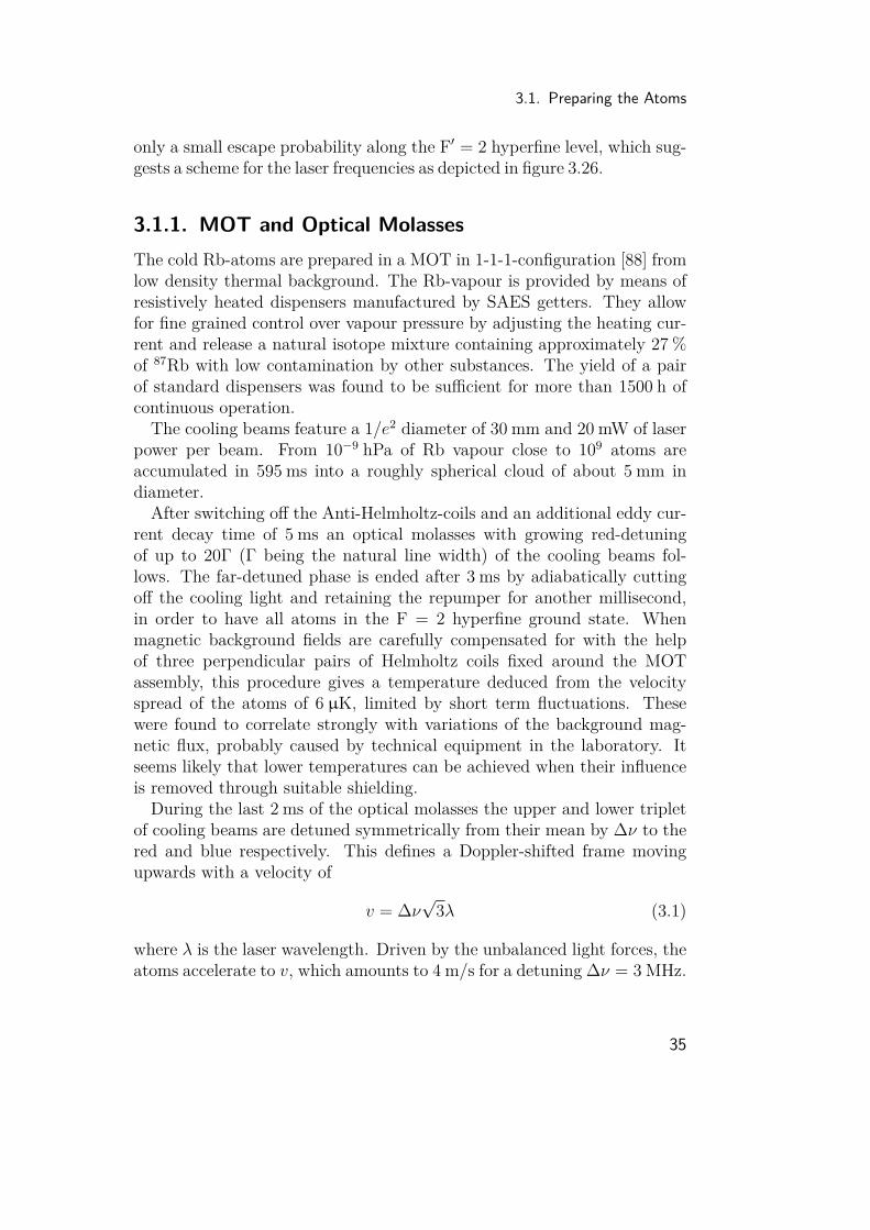
Figure 3.3.: Cut through MOT-chamber, coil and beam-expander.
37

3. Experiment
After switching off the light beams, this motion becomes the startingpoint of a free flight parabola peaking 815 mm above the MOT after408 ms.
0.10
0.11
0.12
0.13
0.14
0.15
−60−40−20 0 20 40 60Frequency [kHz]
PMT
signa
l [ar
b. u
nits
]
0.100.120.140.160.180.200.220.24
−300 −200 −100 0 100 200 300
Figure 3.4.: (left) By scanning the difference frequency between the co-propagating Raman beams, magnetic sublevels can be selectively addressed.As both co-propagating beams feature the same polarization (σ±), only tran-sitions with equal magnetic sublevel in the initial and final state are allowed.Starting from |F = 2〉, three sublevels in |F = 1〉 are available and thus threepeaks are observed. The shown frequency splitting is equivalent to a magneticflux present at the location of the atoms of 7.2 µT. (right) A closer look ata single resonance reveals a structure well described by Rabi transitions withfixed pulse-length and variable detuning. For this measurement a shorter π-pulse with square enveloped was applied, in contrast to the otherwise usedGaussian pulses.
The vacuum chamber for the MOT was designed with the special de-mands of a transportable and rugged device for field use in mind. Tominimize overall size, and to maximize number and diameter of viewports,an approach was taken where the entire chamber is milled from a singleblock. The material of choice is a titanium alloy, as the low density re-sults in low weight (≈ 14 kg), even if larger quantities of metal are presentwhen compared to chambers welded together from tubes. An additionaladvantage is the low specific conductivity, resulting in high ohmic resis-tance and therefore short decay times for eddy currents. It was found thatthe switch-off time for the MOT-fields is shorter than 5 ms with the ratherlarge cross-sections in place depicted in figure 3.3.
38

3.1. Preparing the Atoms
Two cylindrical recesses were cut into the chamber where the Anti-Helmholtz-coils wound on slitted copper bobbins are mounted concentri-cally to a pair of opposing cooling beams. This configuration gives a mag-netic flux gradient of 0.5 mT/cm at a current of only 8 A in the regionof the MOT, which eliminates the need for cumbersome water cooling.
4 cm
Figure 3.5.: Vacuum Pivot exploded (left) and in assembled form (right).
The cooling beams are delivered by folded collimators attached directlyto the window caps holding the optical flats, which serve as view-ports.The collimators are designed to expand the cooling light coupled throughpolarization maintaining fibres to a diameter of 30 mm in a space-efficientway (f-number 3.6, still reasonably good beam quality, overall dimensions50× 50× 130 mm3). Special care was taken to use only materials withµ ≈ 1 to keep magnetic interference low.The collimators also allow for precise steering of the beam through the
chamber (six degrees of freedom), which is useful for initial alignment ofthe MOT beams. Here one triplet is first set to propagate colinearly withthe respective boreholes, in order to profit from tight machining toleranceswhen adjusting perpendicularity. The other triplet is then aligned so thatevery beam is anti-parallel to its opponent by maximising mutual couplinginto the fibres. In a last step all beams are tilted vertically by 3 mrad toavoid large scale interference patterns, which were found to give unstableMOT conditions.Afterwards, the collimators can be locked as the orientation of the atomic
fountain is tuned by rotating the whole MOT-chamber around a point de-fined shortly above the chamber with a vacuum pivot. The pivot was
39

3. Experiment
designed to allow for angular movements with very low friction. As con-ventional parts often contain magnetizable components, ball-bearings madefrom glass and nylon were chosen. With only a small load acting on them(the weight of the MOT-chamber is almost fully compensated by the pres-sure difference), the bearings could be pre-stressed by fitting them snuglyinto suitable holding fixtures. The resulting action free of play and stick-slip enables angular adjustments with high precision. Using suitable ac-tuators, the pointing can be set with a resolution < 10 µrad, equivalentto a displacement of ≈ 30 µm of the atomic cloud in the detection area.This ability becomes important, when the effect of Coriolis forces is to becompensated, see section 4.2.
3.1.2. Velocity Selection1 ms after launching the atoms, the z-component of the compensating mag-netic field is ramped up to 120 µT. This way, a quantization axis parallel tothe linearly polarized Raman-beams is defined, which propagate verticallyfrom top to bottom and are back-reflected of a horizontal mirror below theMOT-chamber. A properly aligned λ/4-plate in front of the mirror givesa linear polarization of the reflected beams perpendicular to the incidentpolarization. Restricted by polarization selection rules this lin-lin config-uration only drives Raman-transitions stimulated by counter-propagatingbeams. From the two pairs present a specific set is chosen by tuning thefrequency difference to the Doppler-shifted resonance of the atoms movingupwards.A π-pulse with a Gaussian envelope of width 56 µs selectively transfers
only atoms with the proper velocity component along the vertical axisto |F = 1〉 [89], whereafter the remaining atoms in |F = 2〉 are scatteredaway by a short pulse of one of the cooling beams. The Fourier-width of theRaman-pulse corresponds to a momentum spread of 1/10th of the recoilmomentum of the transferred atoms. This is in fulfilment of the conditionfor negligible dispersive effects of thick beamsplitters and also improves theachievable fringe contrast. It further ensures that the vertical size of theatomic cloud is virtually constant over the course of a shot, which helps indetection, as clipping effects are avoided.The frequency-selective Raman-pulse is also a useful tool to quantify
the magnetic flux in the MOT-region. The Zeeman-splitting of the atomscan be resolved (figure 3.4) by scanning the difference in frequency of thetwo beams in a Doppler-insensitive configuration, obtained by switchingthe beams to circular polarization and blocking the bottom mirror. As
40

3.1. Preparing the Atoms
the magnetic sub-levels of both hyperfine levels split by equal but oppo-site amounts when a certain flux is applied, a net difference of 14 kHz/µTbetween adjacent sub-levels is the result. The resolution of this method issub-µT, as the Raman pulses have a Fourier-width of 2.8 kHz.Even more useful than scanning is a "real-time" method, where a single
pulse (now back in Doppler-sensitive mode) resonant with the mean veloc-ity of the cloud is applied. This selects three classes of atoms, as those insub-states mF 6= 0 are preserved when their Doppler-shift is compensatedby the corresponding Zeeman-shift. The three classes have slightly differ-ent velocities, which leads to a spatial splitting at the end of the free-flightparabola. When the atoms pass through a narrow detection beam, aneasily resolvable time pattern is observed, where the temporal splitting isproportional to the Zeeman splitting. Overlapping the pulses during detec-tion by adjusting the compensation coils guarantees for good cancellationof background fields.Another advantage of the second method is the much higher temporal
resolution as well as a crude guess of the atom’s temperature, which canbe gathered from the height of the detection signal. Higher temperaturesof the atomic sample mean a higher spread in the velocities and thus alower signal, as less atoms fulfilled the tight velocity constraints of theRaman pulse. This allows for an in situ examination of the magnetic fluxfluctuations in the MOT, which enabled to identify magnetic noise as themain obstacle to lower temperatures. This was deduced from a strongcorrelation found between fluctuations in residual Zeeman-splitting, signalheight and the signal of a pick-up coil.
3.1.3. State SelectionIn order to minimize unwanted phase shifts caused by inhomogeneous strayfields in the interferometer zone, the atoms need to be prepared in themagnetically insensitive sub-state mF = 0. Optical pumping would in-volve multiple scattering of photons, leading to considerable heating of theatoms. A better approach is to discard all atoms in wrong sub-states,which also serves to clean the sample from residual velocity componentscaused by atoms in sub-states mF 6= 0.State selection takes place in the central part of the vacuum system,
again machined from bulk material. A chamber with 8 windows on itsoctagonal perimeter in the horizontal plane allows multiple optical ac-cess to the atomic cloud in its middle. Two axes (4 windows) are usedfor detection, while one of the remaining windows serves as a microwave
41

3. Experiment
port. A coaxial-to-wave-guide-adapter (Omecon RA-14-PQB-012-B-SMA-F) mounted to the window cap couples ≈ 2 W of microwave radiation res-onant with the D2-hyperfine splitting into the viewport. The wave travelsthrough the chamber and is reflected back by an aluminium mirror fixedto the opposing side, so that the amplitude of the standing wave at thecentre of the chamber can be maximised by adjusting its position. A sin-gle microwave π-pulse with a width of 45 µs is preceded by 1 ms×10 mWof light resonant with the (F = 2 ↔ F ′ = 3)-transition and backed by5 ms×1 mW tuned to (F = 1 ↔ F ′ = 0). The light is delivered by abare fibre and fed through a hole in the back of the microwave coupler,from where it is allowed to diverge into the chamber. With a magneticflux of 100 µT and suitable orientation of the linearly polarized microwaveat the location of the atoms, only those initially in |F = 1,mF = 0〉 areleft in |F = 2,mF = 0〉, while all other atoms gather additional horizontalmomentum by the scattered light and get lost.
3.2. Interferometer Sequence
3.2.1. Magnetic FieldsThe well defined sample of cold atoms enters then the interferometer zoneformed by a 750 mm long titanium tube with a diameter of 40 mm mountedat the top of the vacuum system. A vertical quantization axis is providedby the field of a cylindrical coil wound on an aluminium cylinder coveringthe whole length of the tube. Two helical groves with opposing directionof rotation, a precise pitch of 3 mm per turn and a diameter of 70 mm weremachined on its outer mantle to define the exact position of the windings.This technique gives minimal spatial variations of the magnetic flux whileit is possible to suppress the small horizontal component generated by ashort coil when interconnecting the two helices with a current going frombottom to top along one of the windings and down along the other. Both,the interferometer tube and the quantization field coil are contained in acustom magnetic shield designed by The Mushield company. It consists ofthree equally spaced concentric cylinders made from 0.75 mm thick sheetsof high-permeability nickel-iron-molybdenum alloy. The innermost cylin-der has a length of 675 mm and a diameter of 79 mm while the outermostis 723 mm long and 130 mm wide with the middle and outer cylinder capedto the open diameter of the inner cylinder. For a volume close to its cen-tre the shield provides an attenuation factor of roughly 1000 for magnetic
42
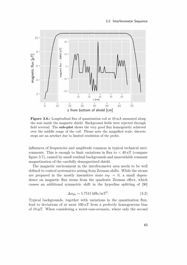
3.2. Interferometer Sequence
z from bottom of shield [cm]
mag
netic
flux
[µT]
2
4
6
8
10
0 10 20 30 40 50 60 70
z [cm]
mag
netic
flux
− 1
0655
[nT]
−20
−10
0
10
20
20 30 40 50 60
Figure 3.6.: Longitudinal flux of quantization coil at 10 mA measured alongthe axis inside the magnetic shield. Background fields were rejected throughfield reversal. The sub-plot shows the very good flux homogeneity achievedover the middle range of the coil. Please note the magnified scale; discretesteps are an artefact due to limited resolution of the probe.
influences of frequencies and amplitude common in typical technical envi-ronments. This is enough to limit variations in flux to < 40 nT (comparefigure 3.7), caused by small residual backgrounds and unavoidable remnantmagnetization of the carefully demagnetized shield.The magnetic environment in the interferometer area needs to be well
defined to control systematics arising from Zeeman shifts. While the atomsare prepared in the mostly insensitive state mF = 0, a small depen-dence on magnetic flux stems from the quadratic Zeeman effect, whichcauses an additional symmetric shift in the hyperfine splitting of [90]
∆νhfs = 5.7515 kHz/mT2. (3.2)Typical backgrounds, together with variations in the quantization flux,lead to deviations of at most 100 nT from a perfectly homogeneous biasof 10 µT. When considering a worst-case-scenario, where only the second
43

3. Experiment
half of the sequence is affected by the erroneous flux—which geometricallyis not possible for the π-pulse close to the apex—this would give rise to aphase shift of
∆φquad ≈ ∆νhfs10 µT 100 nT 0.25 s = 1.4mrad. (3.3)
Because both paths are always close together with respect to the lengthscale of flux variations and because the interferometer is almost sym-metric to the apex, the real phase shift is much lower and thus negligi-ble.As a quadratic dependence on the bias flux can be expected for the
strength of errors caused by irregularities of the coil, it might be that muchhigher settings are connected to measurable shifts in the interferometerphase. Such higher flux would be necessary to completely separate atomsin sub-states other thanmF = 0 in the frequency domain, when rectangularRaman pulses with typical lengths of 25 ms for π/2 are used. With thecomparatively low setting at hand, undesirable mixing between adjacentsub-states is the consequence e. g. for not perfectly linear polarizationsof the Raman beams. Careful state-selection of the atoms is therefore aprerequisite for accurate measurements.In order to avoid edge effects of the quantization coil and of residual fields
leaking through the apertures of the shield, the interferometer sequenceshould be limited to the length of the vacuum tube reduced by 150 mm ateach end. This gives a vertical space of 450 mm equivalent to a free falltime of 600 ms. The largest temporal separation T of the interferometerpulses is therefore 275 ms, if a minimal distance from the apex of 15 msis chosen to ensure unambiguous addressing through adequate Doppler-shifting. The rather long tube makes it also possible to use shorter T andstack two simultaneous interferometers on top of each other by "juggling"the cold clouds [47], which should enable measurements of the Gravitygradient.
3.2.2. Raman BeamsThe light for the Raman beams is delivered by a polarization maintain-ing fibre with both frequencies ω1, ω2 sharing the same linear polariza-tion. A beam-expander (60FC-T-4-M200-37 by Schäfter+Kirchhoff) isused, where the light is allowed to expand freely after leaving the fibreand is collimated by an achromatic lens to an 1/e2-diameter of 29.5 mm,when using a fibre with a numerical aperture NA(5%) = 0.09. The lens is
44

3.2. Interferometer Sequence
z [cm]
resid
ual m
agne
tic fl
ux [n
T]
20406080
100
32343638404244
20 30 40 50 60
backgroundm
agnetization
Figure 3.7.: Small flux in the magnetic shield due to remnant magnetiza-tion and residuals of typical background fields in a technical environment.Measured with a fluxmeter and separated through flipping the shield.
designed to give a wavefront aberration of λ/20 over the aforementionedaperture, while the beam diameter is chosen to minimize stray light andwavefront perturbations caused by the beam clipping at various openingsof minimal ∅ = 40 mm in the vertical beam-path through the appara-tus.The collimated beam enters and leaves the vacuum-system through 50 mm
diameter optical flats with an antireflection coating specified to better than0.25 % at 780 nm, parallelism better than 1′ and wavefront aberration bet-ter than λ/20. The windows are mounted in soft indium seals and are15 mm thick in order to minimize beam perturbations caused by stress orbending.Below the lower window a λ/4-plate (Laser Components, QWP0-780-
20-4, zero order, flat to λ/10, 10-5 scratch-dig) is mounted in front of avibration-isolated high-quality mirror (BFI Optilas, λ/20, 10-5 scratch-dig), from where the beam is reflected back to the beam-expander. Anadditional λ/4-plate, which can be shifted into the optical path betweenbeam-expander and upper window, will lead to a σ+-σ+ configuration fora pair of co-propagating beams. These can be used to drive Doppler insensi-tive Raman transitions when the back-reflected beams are blocked.
45

3. Experiment
The Raman beams have a power of 40 mW each, which gives pulselengths of 22 µs (π/2) and 44 µs for the rectangular envelope required bytheory. As the velocity-selective pulse was set to be of Gaussian shape withσ = 56 µs (intensity), the remaining Doppler spread of the atoms is wellwithin the Fourier width of the Raman pulses, ensuring that all atoms areequally addressed during the interferometer.
Wavefront Aberrations
The optics involved were chosen to give minimal deviation from perfectplane waves for the Raman beams, but the small perturbations still presentneed some consideration nonetheless. With wavefront radii large enoughto neglect the effect of beam propagation over the dimensions of the ex-periment, the phase errors induced by co-propagating beams will be thesame and thus cancel. In the case of counter-propagating beams thisholds only for wavefront errors caused by optical elements present in bothbeams. Those due to the lower window, the lower quarterplate and themirror, which are traversed only by the retro-reflected beam, are discussedhere.The simplest form of wavefront aberrations are curvatures over the full
aperture, centred on the optical axis, and are considered here, as the treat-ment is straight-forward. The maximal error for the optical elementsused in the Raman beams is specified to be less than δ = λ/20, whichis equivalent to radii of up to some 1000 m for the given beam diameter.The phase difference imprinted into the atom by two counter-propagatingbeams with curved wavefronts is equivalent to that caused by only onebeam carrying the difference in curvature, quantified by δ0 at a radius w0(compare figure 3.8). As the beam is reflected back by a mirror, the errorsdue to any optical element traversed twice will count doubly, thus giving
δ0 ≈ 2∑α
δα + δmirror, (3.4)
where δα of each optical element has a sign depending on the orientation(up or down) of its induced curvature for a beam passing through it in afixed direction. In the situation at hand with two elements (lower windowand retarder plate) plus the mirror, cancelling can not be expected, thuserrors significantly larger than that of a single element are to be consid-ered.For δ0 R the spherical wavefront can be approximated by a paraboloid
and the deviation at a certain distance w from the optical axis can be
46

3.2. Interferometer Sequence
written asδ ≈
(w
w0
)2δ0. (3.5)
When following a single atom through the interferometer sequence andomitting the small splitting of the trajectories, the additional phase shiftdue to wavefront curvature can be expressed as
∆φwfc = 2πλδ0
(w(t1)w0
)2
− 2(w(t2)w0
)2
+(w(t3)w0
)2 . (3.6)
Noting that a cut through a paraboloid of revolution in a plane parallelto the central axis will give an intersection congruent with the revolvedparabola maps the two-dimensional case to a one-dimensional problem.With the ti being equally spaced by T and the movement of the atom ina plane perpendicular to the z-axis being given by a constant velocity vlat,the expression from above reduces to
∆φwfc = 2πδ0
λ
2 (vlatT )2
w20
, (3.7)
which is remarkable for the fact that the phase shift an atom experiencesis independent of its initial position.For laser cooled atoms the distribution of their horizontal velocities is
fixed by the temperature of the cloud after optical molasses. To estimatethe effect of wavefront curvature on gravity measurements, the contribu-tion of all atoms detected after the interferometer sequence is to be av-eraged. In a simple model the atoms are thought to start from Gaussiandistributed points in a disc centred on the optical axis after the coolingbeams have been shut off. After time T , during which their horizon-tal movement is unaffected by the Raman pulses, the atoms are interro-gated by fluorescence detection in a circular area of suitably chosen radiusD.The averaged phase shift is most conveniently expressed as a complex
amplitude factor. Due to the axial symmetry the integrals over startingpoints and velocities can be reduced to 1D-integrals, which gives
Awfc =
∫∞0∫∞
0 γ(r, v)ρ(r, v) exp[i2πδ0
λ
2 (vT )2
w20
]dv dr∫∞
0∫∞
0 γ(r, v)ρ(r, v)dv dr (3.8)
47

3. Experiment
whereρ(r, v) = exp
[−1
2
(r
r0
)2]r exp
[−1
2
(v
v0
)2]v. (3.9)
To reflect that not all atoms with velocity v originating in a point withdistance r from the axis will be within the detection area at t = T an angleγ is introduced (compare figure 3.8) as
γ(r, v) :=
0 if |r − vT | > D
2π if r + vT < D
arccos
(vT)2
+ r2 −D2
2vT r
else.(3.10)
For r0 = 2.5 mm, T = 0.7 s and δ0 = π/10, numerical integration gives theresult depicted in figure 3.9, where the averaged phase shift is shown asa function of the radius of the detection area for various temperatures ofthe cloud. With D presently being approximately 4 mm the accumulatedphase shift would be about 11 mrad, which is equivalent to 1 × 10⁻⁹ in gand thus too high for the targeted accuracy. As the overall phase growsalmost linearly with the small wavefront deviations at hand, the situationcan be expected to deteriorate significantly when possible local curvaturesseveral times as high are considered.It should be noted that the error does not vanish if the detection radius
is reduced to zero. This might be puzzling at first glance but is understand-able when looking at atoms which enter the detection area from outside itsdiameter with finite velocities. Other techniques to reduce the phase errorwould be to lower the temperature, to shrink the initial diameter of thecloud or to minimize the time between Raman pulses or between launchand detection. All these solutions would necessitate large modifications ofthe apparatus—e. g. to reach significantly lower atomic velocities far moreinvolved cooling techniques like Raman sideband cooling [91] are needed—or would have a negative impact on interferometer performance—as e. g.cold collisions induced by high atomic densities. Mapping of and correctingfor phase deviations of the Raman beams will therefore be a necessary stepin order to reach highest accuracy.The simple model sketched above does not account for wavefront distor-
tions other than small uniform curvatures. In practice there are variousother perturbations to be dealt with, where those caused by small scat-terers seem especially cumbersome. Dust particles do inevitably find their
48
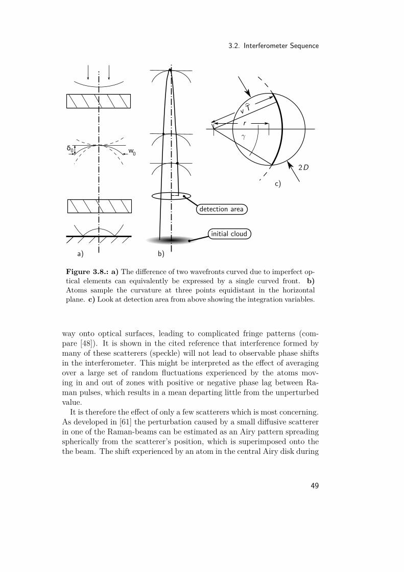
3.2. Interferometer Sequence
r
v T
γ
D
detection area
initial cloud
a) b)
c)
2
wδ0
0
Figure 3.8.: a) The difference of two wavefronts curved due to imperfect op-tical elements can equivalently be expressed by a single curved front. b)Atoms sample the curvature at three points equidistant in the horizontalplane. c) Look at detection area from above showing the integration variables.
way onto optical surfaces, leading to complicated fringe patterns (com-pare [48]). It is shown in the cited reference that interference formed bymany of these scatterers (speckle) will not lead to observable phase shiftsin the interferometer. This might be interpreted as the effect of averagingover a large set of random fluctuations experienced by the atoms mov-ing in and out of zones with positive or negative phase lag between Ra-man pulses, which results in a mean departing little from the unperturbedvalue.It is therefore the effect of only a few scatterers which is most concerning.
As developed in [61] the perturbation caused by a small diffusive scattererin one of the Raman-beams can be estimated as an Airy pattern spreadingspherically from the scatterer’s position, which is superimposed onto thethe beam. The shift experienced by an atom in the central Airy disk during
49

3. Experiment
radius of detection area [mm]
phas
e er
ror [
rad]
0.005
0.010
0.015
0.020
0.025
90nK
360nK
1.4µK
5µK
2 4 6 8
Figure 3.9.: Averaged interferometer phase shift due to wavefront curvatureof the Raman beams. The temperatures shown are equivalent to velocities v0of the atoms of 1/2, 1, 2 and 3.7 times the recoil velocity of 5.9 mm/s.
a Raman pulse is then given by
∆φscat = a2(∆x)2
2λd2skeff (3.11)
where a w0 is the radius of the particle, ds its longitudinal distance fromthe atom and ∆x the lateral offset of the atom from the optical axis, for aparticle centred in the beam. For an estimate of the interferometer phaseshift it is sufficient to consider only a scatterer on the top window disturbingthe downward pointing Raman beam, as the effect drops off with the squareof the distance between particle and atom.The problem is treated similarly to that of uniform curvatures. To ac-
count for a scatterer off the optical axis, the averaging integral needs tobe swept over the angles β and γ (compare figure 3.10), then reading
Ascat =∫∞0∫∞
0∫ 2π
0∫ γ(r,v)−γ(r,v) ρ(r, v) exp
[i∆φscat
]dγ dβ dv dr∫∞
0∫∞0 2πγ(r, v)ρ(r, v)dv dr . (3.12)
50

3.2. Interferometer Sequence
Figure 3.10.: Top view of detection area showing the integration variablesused in the estimation of the effect of a single scatterer in the Raman beam.
where the phase perturbation is due to three light pulses (splitting of thepaths is again neglected)
∆φscat = ∆φscat(t1)− 2∆φscat(t2) + ∆φscat(t3). (3.13)
A slight modification to the phase-factor is necessary to reflect the positionof atom and scatterer, where the latter is rs apart from the optical axis
∆φscat = exp[−1
4r2s − r2
r2beam
]a2rrs2
2λd2skeff. (3.14)
The exponential entering the phase gives the amplitude-ratio of the light atthe positions of scatterer and atom, which together with a factor a2/(dsλ)determines the relative strength of the Airy pattern compared to the Ra-man beam. Numerical evaluation for a particle with a = 20 µm and theπ-pulse situated 15 cm from the top window then gives the result depictedin figure 3.11. For a scatterer on the optical axis the phase shift is accept-able, but grows to cumbersome levels with the particle moving outwardsdue to the comparatively strong curvature of the perturbation. Shiftingthe fountain away from the window strongly lessens the error due to thesensitive dependence of ∆φscat on ds, but this effect is compensated quickly
51

3. Experiment
by growing the scatterer. Dust particles with a radius larger than 100 µmare not uncommon—especially under field conditions—which would giverise to impermissible errors in gravimetric measurements. Therefore con-siderable effort has been made to encapsulate all elements of the opticalpath the Raman-beams take after leaving the fibre.
distance scatterer from z−axis [mm]
phas
e er
ror [
rad]
−0.015
−0.010
−0.005
0.000
2mm
detection radius 8mm
0 2 4 6 8 10
Figure 3.11.: Interferometer phase shift experienced by an atom due to asmall scatterer on top window perturbing the Raman beams. While the radiusof the detection area does have a small influence, variation of temperature isof negligible effect.
Gouy Phase
Two points on the optical axis far away from and on opposite sides of thewaist along a Gaussian beam show a phase difference of π additional to thephase accrued due to beam propagation. In terms of the Rayleigh range itcan be expressed as
ζ(z) = arctan(z
z0
). (3.15)
52
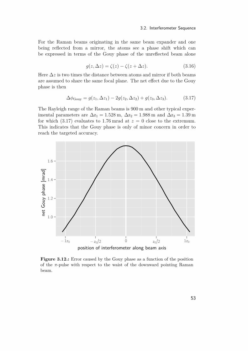
3.2. Interferometer Sequence
For the Raman beams originating in the same beam expander and onebeing reflected from a mirror, the atoms see a phase shift which canbe expressed in terms of the Gouy phase of the unreflected beam alone
g(z,∆z) = ζ(z)− ζ(z + ∆z). (3.16)Here ∆z is two times the distance between atoms and mirror if both beamsare assumed to share the same focal plane. The net effect due to the Gouyphase is then
∆φGouy = g(z1,∆z1)− 2g(z2,∆z2) + g(z3,∆z3). (3.17)
The Rayleigh range of the Raman beams is 900 m and other typical exper-imental parameters are ∆z1 = 1.528 m, ∆z2 = 1.988 m and ∆z3 = 1.39 mfor which (3.17) evaluates to 1.76 mrad at z = 0 close to the extremum.This indicates that the Gouy phase is only of minor concern in order toreach the targeted accuracy.
position of interferometer along beam axis
net G
ouy
phas
e [m
rad]
1.0
1.2
1.4
1.6
−1z0 − z0 2 0 z0 2 1z0
Figure 3.12.: Error caused by the Gouy phase as a function of the positionof the π-pulse with respect to the waist of the downward pointing Ramanbeam.
53

3. Experiment
Beam Alignment
The direction in which the interferometer is sensitive to accelerations isgiven by the wave vectors of the Raman beams. For small deviations θfrom perfectly parallel alignment, the interferometer phase can be writtenas
∆φ = g · keffT2 = gkeffT
2 cos θ ≈ gkeffT2(1− θ2). (3.18)
It is easy to see, that in order to achieve an accuracy ∆g/g of 10−10, θ mustbe less than 10 µrad. Up to a factor of two the same holds for parallel align-ment of the retro-reflected beam with the incident one.
fibre
corner cube
liquid paraffin
CCD
Figure 3.13.: Principle of the procedure used to align the Raman beamsvertical and parallel. By overlapping the focii on the CCD-chip through tiltingof the beam-expander, verticality is achieved. For clarity, not all beams aredrawn.
To ensure proper orientation of the beams a beamsplitter can be insertedbetween Raman beam expander and vacuum system to make use of adedicated alignment tool permanently fixed to the set-up. 50 % of theincident light is directed onto a hollow corner cube, which reflects the light
54

3.2. Interferometer Sequence
back onto the beamsplitter under an angle specified to be less than 5 µrad.The two sides of the beamsplitter are specified to be parallel better than10 µrad, deflecting the light passing through it by less than 5 µrad1. Aplano-convex lens with a focal length of 200 mm is used to focus the lightonto a CCD-chip, salvaged from a simple webcam. The excellent quality ofthe wavefronts allows for a focal waist close to the Rayleigh-limit of 2.5 µm,which about matches the pixel size of the chip. This configuration providesan easy way to control the alignment of the beam down to approximately20 µrad from the picture taken by the camera.A cup filled with liquid paraffin replacing the mirror on top of the vibra-
tion isolation stage below the vacuum system acts as a horizontal reference.The low viscosity of the fluid along with the reduced effect of vibrationsallows to locate the focus of the light reflected from its surface and directedonto the CCD-chip by the beamsplitter to about a pixel. Making the focalpoints of both beams coincide thus guarantees good vertical alignment ofthe Raman beam. Putting the mirror back in its place and adjusting itstilt as to overlap the foci again results in both Raman beams being parallelwithin the requirements.The procedure is limited by the wedge of the lower vacuum window of less
than 1′ which gives an upper bound on verticality of about 150 µrad. Thisis clearly insufficient to achieve the desired accuracy, but provides a goodstarting point to optimize vertical adjustment. Tilting the pair of Ramanbeams will result in the measured value of g being a parabolic function ofthe tilt angle, which allows to identify the correct setting [48].A tilt sensor (Applied Geomechanics, 756-1129) fixed to the mirror from
beneath allows for continuous monitoring of both tilt axes with 1 µradprecision and thus for corrections of the variations caused by the somewhatwobbly vibration isolation. The rigid fixture holding the Raman beamexpander and attached parts on top of the experiment (compare figure 3.19)was designed to provide a stiff base immune to deflection and vibrations.Plates of wooden laminate material were used to further promote stabilityand to minimize ringing, which is a problem with all-metal structures.Regular inspection of the Raman optics showed no significant tilt for theupper optics within the limits of the alignment tool over the course ofmulti-day measurement campaigns.
1For an optical flat with a small wedge made from most common materials, the de-flection angle can be estimated to be roughly half of the wedge angle.
55

3. Experiment
3.3. DetectionThe outputs of the interferometer are read out when the atoms fall backinto the central chamber (compare figure 3.1). For this purpose a sim-ple fluorescence scheme is implemented, where the two hyperfine statesare successively addressed by resonant laser light and a fraction of thescattered photons are collected onto a photomultiplier tube. From theratio of the integrated signals the interferometer phase can then be ob-tained.
3.3.1. OpticsThe detection light is delivered through a fibre from where it passes aquarter-wave plate and is otherwise allowed to expand freely. An achro-matic lens with focal length of 250 mm is used to collimate the beam to a1/e2-diameter of 50 mm, which gives a large central area with almost uni-form intensity in order to minimize spatial dependency of the detection.The actual diameter of the detection beam is set by an iris diaphragmpositioned between fibre and lens and a series of baffles after the collima-tor is used to catch most of the light diffracted at its rims. The beamis then steered through the chamber in a horizontal plane and reflectedback by a mirror on the opposite side to balance light forces acting on theatoms.Light scattered by the cloud is distributed isotropically in all directions
for circular polarization of the detection beam. A solid angle of≈ 4π/100 sris sampled by two plano-convex lenses mounted back-to-back as close to thevertical axis as possible in a dedicated viewport perpendicular to the onesused to deliver the detection light. The combined focal length is chosenas to image the cloud with unity scale onto a slit mounted in front of aphotomultiplier tube (PMT). During measurements, beam diameter andslit aperture are set to select a central volume of 8× 8× 8 mm3 of the cloudin order to minimize systematic effects. Attached to the viewport opposingthe PMT is a horn-shaped light dump which gives an almost completelydark background. Along with the measures to avoid stray light from thedetection beam, this results in a residual signal of the PMT limited byphotons scattered from thermal background vapour.In order to assess the background-signal, which can be as high as the
interferometer signal, the detection scheme described in the following para-graph is implemented twice: a first sequence is applied when the atomsreturning from the interferometer zone are in front of the PMT, and a
56

3.4. Vibration Isolation
second measurement is taken 20 ms later when all atoms from the initialMOT have left the detection area. Simple subtraction then separates thebackground from the interferometer signal.During detection, two pulses of light 400 µs long and red-detuned by
1 MHz to the (F = 2 ↔ F ′ = 3)-transition are separated by 50 µs ofrepumper (F = 1 ↔ F ′ = 2). This pattern subsequently samples thefraction of atoms in |F = 2〉 and then all atoms as those left in |F = 1〉 aretransferred to the other hyperfine ground state during the middle pulse.The intensity is set to the saturation intensity, which results in the PMTreceiving about 60 photons from each atom in resonance. Even for lowquantum efficiencies it is thus ensured that determination of the ratio ofatoms is not limited by photon statistics. The short pulse-lengths werechosen to prevent optical pumping, which would otherwise result in atomsbeing transferred to |F = 1〉 during detection pulses and consequently abias in the observed ratio of atoms.
3.3.2. ElectronicsThe PMT is a Hamamatsu R10699 with a specified quantum efficiency of10 % at 780 nm and an active area of 8× 24 mm2, mounted in a magneticshield. The attached voltage-divider was modified such that the photo-cathode can be shortened to the second dynode at the signal of a TTL-pulse in order to prevent saturation effects during MOT-phase with itsexcessive light levels. The photo current is transduced by a HamamatsuC7319 pre-amplifier unit with a bandwidth of 200 kHz to voltages of a fewvolt. This signal is then sampled with 400 kHz and 16 bit resolution overa range of 20 V and stored for further processing.
3.4. Vibration Isolation2
The interferometer is built to measure very precisely the acceleration ex-perienced by the atoms with respect to the mirror beneath the vacuumchamber, as the latter fixes the frame in which the phase of the effectivewave vector is to be described. The measured acceleration thus equalslocal g only if the mirror is resting with respect to the masses which
2This component of the fountain set-up was developed together with Christian Freierand is part of his diploma thesis [92]. Much of the benefit drawn from the vibrationisolation is due to his excellent work.
57

3. Experiment
are the cause of said gravity3. An important source of erroneous move-ments of the mirror are vibrations of the supporting floor—mostly dueto technical noise abundantly present in human environments, but alsoof natural origin in the form of microseisms caused by ocean waves andwind.The relevant spectrum ranges from roughly 30 mHz given by the lower
end of predominant frequencies found in wave patterns and goes up to aabout 10 Hz defined by the finite bandwidth of the interferometer’s sensi-tivity (compare figure 2.4). Accelerations in this frequency band are readilymeasured with high precision by commercially available seismometers andcan in principle be removed retrospectively from gravity data [93, 94]. How-ever, it was found to be more reliable and efficient to reject accelerationnoise during measurements. This is done by placing the mirror on top ofa vibrationally isolated stage formed by a passive spring system enhancedwith an active feedback loop to lower its eigenfrequency. A similar systemwas employed in an earlier gravimeter and proved to be a key componentto reach competitive performance [95].Common vibration isolation systems are based on the observation that a
mass coupled elastically through a spring to a moving foundation will followthe motion with progressively lower amplitude for frequencies higher thanthe (highest) eigenfrequency of the oscillatory system formed by springand mass. The simple example of a mirror suspended from a tension springcould in principle be applied to the task at hand. But to reach a sufficientlylow eigenfrequency a spring over 250 m long would be needed, which doesnot agree well with the constraints of a mobile apparatus. Instead, a devicehad to be designed to fit into the available space of about 40× 40× 30 cm3
and be rugged enough for field use.
3.4.1. MechanicsThe foundation of the system is the commercial isolation stage 50BM-10by MinusK Technology, measuring 30× 30× 12 cm3 and weighting about16 kg. Utilizing a patented mechanism it features a vertical resonance aslow as 0.5 Hz for masses of up to 25 kg on top of its platform. In order to
3As Earth itself is a rather wobbly affair if looked at scrupulously, it is hard to tell whatexactly the reference should be to which the mirror is to be tied. To the best of theauthor’s knowledge "local gravity" is in practice defined as the effect left over whenall known sources of error are removed. This approach in turn seems somewhatflawed by not always fully established conventions of what to count as error; seediscussions related to "permanent tide".
58
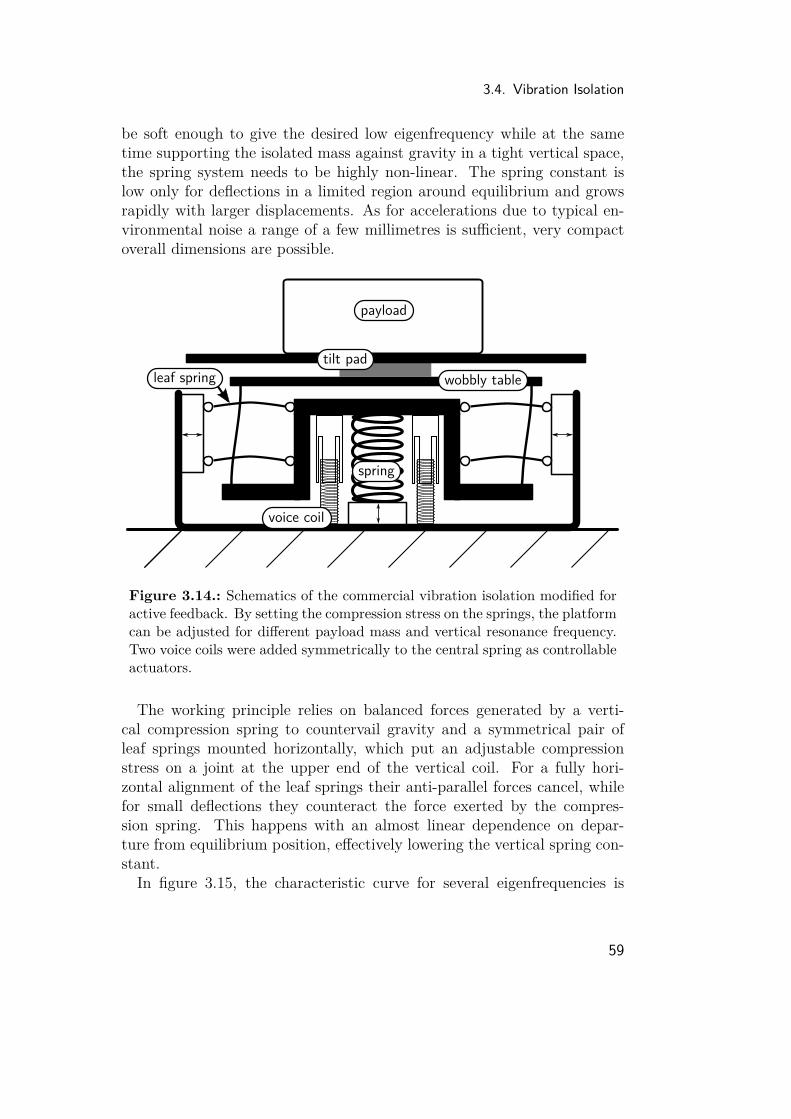
3.4. Vibration Isolation
be soft enough to give the desired low eigenfrequency while at the sametime supporting the isolated mass against gravity in a tight vertical space,the spring system needs to be highly non-linear. The spring constant islow only for deflections in a limited region around equilibrium and growsrapidly with larger displacements. As for accelerations due to typical en-vironmental noise a range of a few millimetres is sufficient, very compactoverall dimensions are possible.
spring
voice coil
payload
wobbly table
tilt pad
leaf spring
Figure 3.14.: Schematics of the commercial vibration isolation modified foractive feedback. By setting the compression stress on the springs, the platformcan be adjusted for different payload mass and vertical resonance frequency.Two voice coils were added symmetrically to the central spring as controllableactuators.
The working principle relies on balanced forces generated by a verti-cal compression spring to countervail gravity and a symmetrical pair ofleaf springs mounted horizontally, which put an adjustable compressionstress on a joint at the upper end of the vertical coil. For a fully hori-zontal alignment of the leaf springs their anti-parallel forces cancel, whilefor small deflections they counteract the force exerted by the compres-sion spring. This happens with an almost linear dependence on depar-ture from equilibrium position, effectively lowering the vertical spring con-stant.In figure 3.15, the characteristic curve for several eigenfrequencies is
59

3. Experiment
given. While with care resonances even lower than 0.4 Hz are achievable,the system exhibits a growing tendency to drift from equilibrium positiontowards one of the ends of the soft range as the springs react to minutechanges of their temperature and creep in the system. This limits the use-ful interval of settings to above 0.6 Hz if long-term stability is needed. Forthe isolation platform being part of the active feedback loop an even higherfrequency of 0.8 Hz was chosen to diminish hysteresis and other nonlineareffects which otherwise might compromise feedback characteristics. A mod-est hardening of the spring system for greater elongations was found useful,though, to limit run-away caused by transients.
force [N]
elong
atio
n [m
m]
−1.5
−1.0
−0.5
0.0
0.5
1.0
1.5
0.93 Hz0.73 Hz
0.54 Hz
0.34 Hz
−0.4 −0.2 0.0 0.2 0.4
Figure 3.15.: Elongation vs. force exhibited by the negative-stiffness mech-anism employed in the vibration isolation. Pronounced hysteresis appearswhen the system is made softer to obtain lower eigenfrequency. Wiggles inthe curves are an artefact caused by the platform "bumping into" the springbecoming swiftly stiffer.
The isolation stage also features suppression of horizontal vibration bymeans of supporting a rigid plate on top of four thin rods at its corners.This inverted-pendulum configuration—nick-named a "wobbly table"—re-lies on the restoring force exercised by the rods clamped at both ends
60
3.4. Vibration Isolation
when deflected in the course of the plate departing from its horizontalequilibrium position. Originally the rods were fabricated as to providea natural frequency of about 1.5 Hz for supported masses close to 25 kg.Upon request the manufacturer provided custom rods which produce aresonance at 0.5 Hz for a similar mass. This helped in alleviating crosscoupling effects found to occur at larger horizontal amplitudes excited ifthe horizontal eigenfrequency of the platform coincided with resonances ofthe building at 1.7 Hz.Mounted in between the "wobbly table" and the top plate is a pad of
visco-elastic polymer roughly 4× 4× 1 cm3 in size. It is promoted as "tiltpad", suggesting that its purpose is the suppression of oscillatory tilt modes.Additionally it was found to be crucial in damping noise due to eigen-modes of the vibration isolation between 10 and 50 Hz which otherwisewould badly compromise isolation performance. Albeit the effect on tiltstability—important for the performance of the interferometer—is detri-mental, its benefits were found to outweigh its drawbacks. Therefore initialtilt of the top plate has to be nulled by careful positioning of the masses andsubsequent creep is to be monitored with a tilt-sensor.A second effect of the tilt pad is an additional sharp resonance produced
at 100 Hz. While direct implications for the interferometer are negligiblethis is still cumbersome since the connected phase shift limits the feedbackgain applicable for frequencies larger than a few Hertz. Until a remedyis found, the effect needs to be incorporated into the model from which adesign of the active vibration isolation system is to be derived. Evaluationof the response to oscillations stimulated by the voice coils suggests, that itcan be best described as a hysteretically damped oscillator with a transferfunction
G(ω) = ω20
1 + i tan(β)ω2
0(1 + i tan(β))− ω2 . (3.19)
where the parameter β was derived from fits to be 0.17 rad [92].To enable active control of the platform, two voice coils (PBA, ∅16 mm,
length when in central position is 31 mm) were mounted between baseand upper end of the vertical isolation stage (compare figure 3.14) sym-metrically to the compression spring. Their combined force exerted at amaximum coil current of 1.5 A is 6 N, much larger than the 200 mN esti-mated to compensate for residual accelerations in the frequency band up to100 Hz acting on a mass of 20 kg. An additional LVDT sensor (SolartronOP6) placed in another corner allows for friction-less monitoring of thevertical displacement with micrometre resolution.
61

3. Experiment
An integral part of the feedback loop is a Güralp CMG-3VL seismometercustomized to provide a flat acceleration response of 2 kV/(ms2) over therange of 0.003–100 Hz on top of the MinusK-platform. The seismometer isa uni-axial sensor with a cross coupling rejection of > 65 dB and equiva-lent self-noise below what is found at the seismologically quietest sites onEarth. Its cylindrical housing made from mild steel measures 101.6 mm indiameter and 208 mm in height. Mounted to its upper end in a tube fittedto a stable kinematic mirror mount is the retro-reflector assembly com-prising the mirror with quarter-wave plate and the tilt-sensor, comparefigure 3.18.To prevent cross-coupling of residual horizontal and tilting accelerations
into the seismometer signal, careful alignment is necessary. The naive ap-proach would be to place the seismometer exactly vertical in the middleof the platform. But it was found in earlier work [95], that the positionof the actual sensor inside the housing is slightly asymmetric. By subject-ing the seismometer to tightly controlled angular motions it was confirmedthat for this specimen the sensitive axis is indeed centrosymmetric. Theseismometer was also tested for sensitivity to horizontal motions, whichrevealed a disconcerting angle of 18 mrad, by which the device had tobe tilted to minimize cross-coupling. Consultation with the manufacturerdisclosed the possibility of severe misalignment during assembly, whichan improved design of the seismometer is expected to forbid in the fu-ture.
3.4.2. Feedback LoopThe bare vibration isolation as bought from MinusK is described well asan under-damped spring-mass system with a natural frequency of here0.8 Hz. Vibrations of lower frequency will pass through essentially unsup-pressed while for higher frequencies the amplitude decreases initially withω−2 and above a frequency depending on the amount of damping (typically2π ∗ 10 Hz) with ω−1. This gives a mean attenuation of only a factor 10in the important range from 1 to 10 Hz and even an amplification of thevibrations close to resonance. To extend the band over which transmissionis decreased—which simultaneously lessens the transmitted amplitude inaforementioned range—an active feedback loop was implemented. The un-derlying idea is to measure the residual accelerations on the platform and toapply a proportional force counteracting the force of the spring, effectivelylowering its spring constant k. This is the feedback control analogue tothe negative stiffness technique realized in the MinusK-platform by purely
62

3.4. Vibration Isolation
mechanical means.In mathematical form this principle is readily expressed as
(1 +K)z + 2γω0(z − zg) + 2Hω0z + ω20(z − zg) = 0 (3.20)
which basically is the well-known differential equation of a harmonic oscil-lator at position z with viscous damping, where position (zg) and motion(zg) of the supporting ground with respect to a fixed reference are ac-counted for. ω0 = k/m denotes the unperturbed resonance frequency andγ the damping ratio which is rather small (typically < 0.1) for the Mi-nusK platform. Two terms have been added to reflect the influence offeedback: Kz is due to the force Fa = −mKz exerted by the voice coilsto counter-act the mechanical spring, and a second term according to aforce Fv = −2mω0Hz needs to be introduced to adjust viscous damping.The latter is necessary as without, the damping ratio of the system in-loopwould be γ = γ/(1+K), leading to excessively sharp resonances. The newunperturbed eigenfrequency can be expressed as ω0 = ω0/
√1 +K, which
is exactly the desired result.For K,H being constants, the feedback-loop would easily be realized
with the help of a simple amplifier and an integrator switched between seis-mometer and a voltage-controlled current source to drive the voice coils.The situation becomes more complicated with the high proportional gainK ≈ 300 necessary to achieve the targeted reduction in resonance fre-quency. As signals inevitably suffer from phase shifts caused by the verynature of platform, seismometer and voice coils when passing through theloop, some frequency components will not be attenuated but amplified,since the corresponding feedback is nearly in phase with the perturbation.This leads to unwanted oscillations for certain amplitude conditions, typi-cally when the closed-loop gain is close to or larger than unity. Therefore,to achieve maximum performance, careful design of the feedback param-eters is necessary. The goal is to raise the gain maximally over a rangeas wide as possible, but to keep it low where the phase shift approachesor exceeds ±π. This task has been undertaken and described in [92] andyields the result shown in figure 3.16.The gain becomes a complex-valued function of frequency and substi-
tutes the parameters K and H. The resulting open-loop transfer functionshows the combined effect of the seismometer, processing filters to im-plement the gain function and voice coils together with the response ofthe mass actuated by the isolation platform. As its phase shift alwaysstays within safe operation limits in the range of frequencies with feed-
63
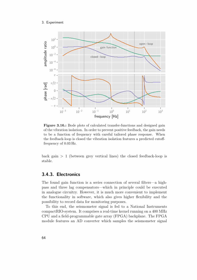
3. Experiment
ampl
itude
ratio
10−6
10−4
10−2
100
102
open−loopgain function
closed−loop
frequency [Hz]
phas
e [ra
d]
−π
−π 2
0
π 2
π
10−3 10−2 10−1 100 101 102 103
Figure 3.16.: Bode plots of calculated transfer-functions and designed gainof the vibration isolation. In order to prevent positive feedback, the gain needsto be a function of frequency with careful tailored phase response. Whenthe feedback-loop is closed the vibration isolation features a predicted cutoff-frequency of 0.03 Hz.
back gain > 1 (between grey vertical lines) the closed feedback-loop isstable.
3.4.3. ElectronicsThe found gain function is a series connection of several filters—a high-pass and three lag compensators—which in principle could be executedin analogue circuitry. However, it is much more convenient to implementthe functionality in software, which also gives higher flexibility and thepossibility to record data for monitoring purposes.To this end, the seismometer signal is fed to a National Instruments
compactRIO-system. It comprises a real-time kernel running on a 400 MHzCPU and a field-programmable gate array (FPGA) backplane. The FPGAmodule features an AD converter which samples the seismometer signal
64
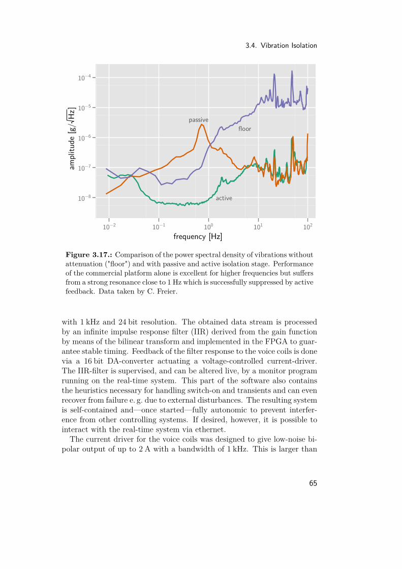
3.4. Vibration Isolation
frequency [Hz]
ampl
itude
[g/
Hz]
10−8
10−7
10−6
10−5
10−4
passivefloor
active
10−2 10−1 100 101 102
Figure 3.17.: Comparison of the power spectral density of vibrations withoutattenuation ("floor") and with passive and active isolation stage. Performanceof the commercial platform alone is excellent for higher frequencies but suffersfrom a strong resonance close to 1 Hz which is successfully suppressed by activefeedback. Data taken by C. Freier.
with 1 kHz and 24 bit resolution. The obtained data stream is processedby an infinite impulse response filter (IIR) derived from the gain functionby means of the bilinear transform and implemented in the FPGA to guar-antee stable timing. Feedback of the filter response to the voice coils is donevia a 16 bit DA-converter actuating a voltage-controlled current-driver.The IIR-filter is supervised, and can be altered live, by a monitor programrunning on the real-time system. This part of the software also containsthe heuristics necessary for handling switch-on and transients and can evenrecover from failure e. g. due to external disturbances. The resulting systemis self-contained and—once started—fully autonomic to prevent interfer-ence from other controlling systems. If desired, however, it is possible tointeract with the real-time system via ethernet.The current driver for the voice coils was designed to give low-noise bi-
polar output of up to 2 A with a bandwidth of 1 kHz. This is larger than
65

3. Experiment
the relevant frequency range of the feedback-loop by a factor of 10 andguarantees that phase shifts are negligible, making this device one of thelongingly desired "set-and-forget"-type.Suppression of vertical floor vibrations is documented in figure 3.17.
While the passive isolation alone is efficient in reducing accelerations on theplatform for frequencies higher than 4 Hz, its narrow resonance produces acumbersome amplification of vibrations around 0.5 Hz. The active feedbackintegrated into the system is highly effective in subduing the resultingoscillations and extends the range of attenuated frequencies by two decadesdown to 0.03 Hz. For frequencies higher than a few Hertz the performanceis close to the original systems as feedback gain trails off. It should be notedthat the curve for the active vibration isolation was obtained in-loop andthus does not necessarily reflect the actual residual vibrations experiencedby the mirror on top of the seismometer. However, corresponding resultsfrom gravimetric measurements strongly suggest equivalent reduction inerroneous accelerations, compare sub-section 4.1.1.
3.5. Fountain Set-up and MobilityDuring the MOT, as well as the free flight phase, the atoms have to be con-served from collisions with thermal atoms e. g. from background vapour asthis is equivalent to a loss of the effected particle. This requires ultra-highvacuum of the order of 10−9 hPa or lower, necessitating particular attentionduring the design of the transportable chamber.Pumping is achieved by a commercial ion pump (Varian Star Cell, 20 L/s
at flange) and a titanium sublimation pump realized in a vertical tubewith ∅70 mm and a height of 280 mm attached on opposite sides to thecentral chamber. The latter also acts as kind of a gate-way with theUHV-valve for external access mounted to its upper end. These typeswere chosen for being vibration-free and—in the case of the sublimationpump—being capable of sustaining the vacuum for at least several dayswithout electrical power. Their combined pumping speed at the centralchamber is estimated to 20 l/s when conduction losses are taken into ac-count.Most parts of the system were made from titanium alloys, which are
known for their good vacuum compatibility, excellent mechanical proper-ties, low density and a magnetic permeability close to unity. Together withthe choice of other building materials to be aluminium and stainless steel ofthe variant EN-1.4406, which also feature low magnetic permeability, the
66

3.5. Fountain Set-up and Mobility
vacuum pivot
detection
Raman beam expander
mirror and quarter plate
magnetic shield
vibration isolation
MOT assembly
µ-wave
vacuum pumps
Figure 3.18.: Vacuum system and attached parts necessary to generate anatomic fountain and perform gravimetric measurements. The set-up is shownfrom two angles. The parts of the experiment which provide laser light andmicrowave along those needed for controlling are housed in separate trolleyframes.
67
3. Experiment
vacuum system can be considered almost amagnetic, perturbing only mini-mally any magnetic flux needed to control the atoms.Welding is cumbersome with titanium due to the high reactivity of the
material to oxygen and the resulting embrittlement. It was unavoidablewith the tube forming the interferometer zone and needed the attention of acompany specialized to this task. With the MOT-chamber and the centralchamber this technique could be avoided by milling each from a single blockof titanium alloy, which also gives compact outer dimensions. A constraintof the bulk-method is that 3 mm of wall thickness should not be under-run to avoid possible leakage through small voids. These inevitably formduring casting in the rods used as starting product.Of special concern were the many view-ports necessary for optical ac-
cess to the atoms. Commercial products of the desired optical and mag-netic properties are expensive and often rely on soldering the glass pieceto a metal sleeve, which can introduce mechanical stress and birefringence.Additionally, the flanges holding the window need to support further equip-ment fastened to them, which forbids the use of copper-gasket sealed CF-flanges. As the copper yields to the induced stress, leaks might form, whichcould compromise vacuum to an unacceptable level.Instead, an approach was used where optical flats are pressed into a soft
metal seal sitting in flat recesses machined into the chambers. The windowcap holding the glass in place is bolted firmly to the chamber in this pro-cess, enabling it to carry high loads. An improved technique—describedin appendix B—was developed, with the potential to outperform similarmethods in the future. However, due to technical problems and tight sched-ules, sealing the windows to the chamber with soft indium wires [96] wasused instead.One of the drawbacks with indium is its low melting point of 157 C,
which prohibits high bake-out temperatures and necessitates additionalcare when cleaning and preparing the vacuum parts. After several weeks ofbaking at 145 C the residual pressure could be lowered to a few 10−10 hPa.An integrated leak rate of less than 10−10 hPa l/s, together with a pumpingspeed of 20 l/s, ensures that pressure returns to similar levels even afterflooding the chamber with Rb-vapour at pressure levels typically ten timesas high during multi-day measurement campaigns.The vacuum system along with the attached optics and auxiliary parts
has a mass of≈ 80 kg. In order to be easily transportable it is mounted on atrolley frame build from aluminium profiles (ITEM Building Kit System)of similar mass running on air-filled heavy-duty wheels. Due to its lowcentre-of-mass the complete package is handled smoothly by two people
68

3.5. Fountain Set-up and Mobility
Figure 3.19.: Fountain set-up mounted in a dedicated undercarriage. Thevacuum system is supported only at the central chamber close to the centreof mass of the complete package, leaving the MOT assembly free to be tiltedto ensure vertical alignment of the atomic fountain.
69

3. Experiment
under more difficult circumstances and can be moved easily by a singleperson on hard, level surface.Validation of mobility was done during moving of the work-group from
the city to Adlershof, a campus situated in the outer rims of Berlin. Thewhole operation went hassle-free and showed the set-up fit for transporta-tion in an ordinary truck with very good stability of vacuum. Deploymentat a new site involves only levelling—which is done by propping the trolleyon three adjustable feet—and vertical alignment, reconnection of power,signal lines and optical fibres and establishment of the vibration isolation.With some exercise this procedure can be accomplished in a few hours,enabling regular relocation of the apparatus. Future enhancements couldeven lead to automation of many of these tasks, which would reduce theeffort of setting-up to pushing a few buttons.
3.6. Gravity of Fountain Set-upWith the mass of the interferometer apparatus approaching 160 kg, thequestion of the magnitude of gravity induced by the experiment itselfsprings to mind. As this systematic effect can hardly be modulated andthus separated from others, it is most useful to calculate the necessary cor-rection. The task at hand is made comparatively easy by the circumstancethat almost all parts of the real set-up have their virtual counterpart in-cluded in a comprehensive CAD-model (compare figure 3.19) as the resultof the design process.Still, with about 700 parts (not counting a few hundred screws) of
roughly 250 different types, manual estimation would be tedious at best.To automate the process, the CAD-assembly was transformed to an AP214 variant of the STEP-model. STEP is meant to be an abstract repre-sentation of all aspects of a product and an open standard promoted bythe ISO. AP 214 is a subset especially useful to describe three-dimensionalgeometries and assemblies thereof. To this end, a product—here the atominterferometer—is represented as a tree with the root node being the com-plete set-up and subsequent nodes constituting sub-assemblies. Conse-quently, the leaf nodes are the single parts from which the apparatus isbuilt and are given in the form of a boundary representation (BREP), thatis their boundary as a set of simple surfaces and lines. Each branch ofthe tree not only acts as the connection between its ends, but also givesinformation of how to position the children by means of rotations and trans-lations with respect to the position of the parent.
70

3.6. Gravity of Fountain Set-up
Figure 3.20.: Tree representation of fountain apparatus. Every end-pointrepresents a single part while intermediate nodes stand for sub-assemblies.E. g. the MOT-assembly can be identified in the right half of the diagram byits six-fold symmetry.
A simple parser was written which crawls the tree to first extract a listof unique parts and subsequently builds a database with their material, oc-currences and according positions in the 3D-set-up and extracts the BREPto be saved into a separate STEP file. In a subsequent step, the BREP ofeach part needs to be transformed into a representation suitable for esti-mating its gravitational effect. A convenient way to do so is to fragmentthe volume enveloped by the BREP into a set of polyhedra, a techniquenamed mesh generation. As it is widely used in finite element methods, arange of powerful tools is available for this purpose.The program of choice is gmsh [97] for being open-source, user-friendly,
scriptable and potent. While optimal mesh generation in two dimen-sions is a solved problem, the same does not hold for three-dimensionalbodies, making some interaction from the user indispensable. However,it was found that with irregular meshes of tetrahedra generated by theMeshAdapt-algorithm in 2D and extended with the Frontal-algorithm to3D, only minor tweaks were necessary to perform the task to a satisfactorylevel in an automated batch-process, for all but a few parts. Mainly somecaution is needed with three-dimensional objects having surfaces whichfeature some kind of singularity, like cones, where—for the purpose of ini-
71
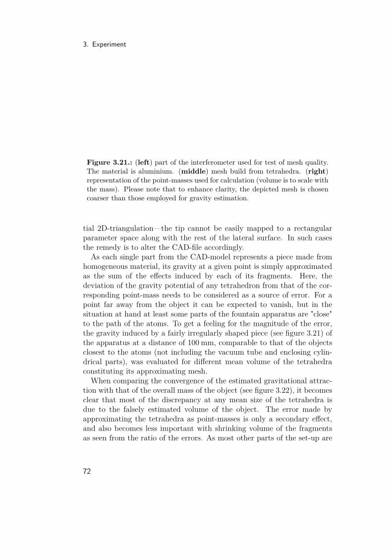
3. Experiment
Figure 3.21.: (left) part of the interferometer used for test of mesh quality.The material is aluminium. (middle) mesh build from tetrahedra. (right)representation of the point-masses used for calculation (volume is to scale withthe mass). Please note that to enhance clarity, the depicted mesh is chosencoarser than those employed for gravity estimation.
tial 2D-triangulation—the tip cannot be easily mapped to a rectangularparameter space along with the rest of the lateral surface. In such casesthe remedy is to alter the CAD-file accordingly.As each single part from the CAD-model represents a piece made from
homogeneous material, its gravity at a given point is simply approximatedas the sum of the effects induced by each of its fragments. Here, thedeviation of the gravity potential of any tetrahedron from that of the cor-responding point-mass needs to be considered as a source of error. For apoint far away from the object it can be expected to vanish, but in thesituation at hand at least some parts of the fountain apparatus are "close"to the path of the atoms. To get a feeling for the magnitude of the error,the gravity induced by a fairly irregularly shaped piece (see figure 3.21) ofthe apparatus at a distance of 100 mm, comparable to that of the objectsclosest to the atoms (not including the vacuum tube and enclosing cylin-drical parts), was evaluated for different mean volume of the tetrahedraconstituting its approximating mesh.When comparing the convergence of the estimated gravitational attrac-
tion with that of the overall mass of the object (see figure 3.22), it becomesclear that most of the discrepancy at any mean size of the tetrahedra isdue to the falsely estimated volume of the object. The error made byapproximating the tetrahedra as point-masses is only a secondary effect,and also becomes less important with shrinking volume of the fragmentsas seen from the ratio of the errors. As most other parts of the set-up are
72

3.6. Gravity of Fountain Set-up
mean tetrahedron mass [g]
norm
alize
d va
lue
1.000
1.002
1.004
1.006
1.008
mass
acceleration
ratio acceleration/mass
10−3.5 10−3 10−2.5 10−2
Figure 3.22.: Total mass and acceleration computed for the test-piece withvarying coarseness of the mesh and scaled to limit value. Both quantities con-verge with growing number of tetrahedra (shrinking mean mass), but the ratioof the quantities close to unity reveals, that the main effect is an improvementin the estimation of the part’s volume and thus mass.
further from the atoms and more regularly shaped, it seems sufficient tochose a mean mass of the tetrahedra of 10 mg to obtain an upper boundon the error of 0.5 %. This approach takes into account that parts madefrom less dense materials e. g. aluminium will also contribute less to thegravity of the apparatus and hence are allowed a slightly larger error bud-get.When meshing the parts of the apparatus, the chosen mean volume
proved also to be the limit feasible with reasonably capable hardware,as more voluminous and complicated parts needed 4 GiB of RAM duringprocessing. The resulting mesh contained up to 106 tetrahedra for thelarger parts (e. g. the MOT-chamber) and a total of 2×10⁷ for the completeapparatus.In a next step, the gravitational acceleration exerted by each building
part was calculated. To this end the corresponding set of point-masses was
73
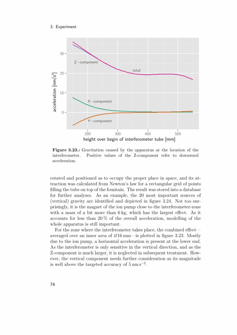
3. Experiment
height over begin of interferometer tube [mm]
acce
lerat
ion
[nm
s2 ]
0
10
20
30
X−component
Y−component
Z−component
total
200 300 400 500
Figure 3.23.: Gravitation caused by the apparatus at the location of theinterferometer. Positive values of the Z-component refer to downwardacceleration.
rotated and positioned as to occupy the proper place in space, and its at-traction was calculated from Newton’s law for a rectangular grid of pointsfilling the tube on top of the fountain. The result was stored into a databasefor further analyses. As an example, the 20 most important sources of(vertical) gravity are identified and depicted in figure 3.24. Not too sur-prisingly, it is the magnet of the ion pump close to the interferometer-zonewith a mass of a bit more than 6 kg, which has the largest effect. As itaccounts for less than 20 % of the overall acceleration, modelling of thewhole apparatus is still important.For the zone where the interferometer takes place, the combined effect—
averaged over an inner area of ∅16 mm—is plotted in figure 3.23. Mostlydue to the ion pump, a horizontal acceleration is present at the lower end.As the interferometer is only sensitive in the vertical direction, and as theZ-component is much larger, it is neglected in subsequent treatment. How-ever, the vertical component needs further consideration as its magnitudeis well above the targeted accuracy of 5 nm s−2.
74
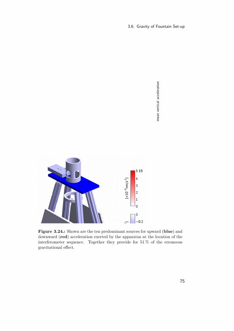
3.6. Gravity of Fountain Set-up
mea
n v
ertica
l ac
cele
ration
Figure 3.24.: Shown are the ten predominant sources for upward (blue) anddownward (red) acceleration exerted by the apparatus at the location of theinterferometer sequence. Together they provide for 51 % of the erroneousgravitational effect.
75

3. Experiment
time [s]
devia
tion
[nm
]
−2.0
−1.5
−1.0
−0.5
0.0 0.1 0.2 0.3 0.4
Figure 3.25.: Difference in the trajectories of the upper path with and with-out the additional gravity of the apparatus. A small splitting of 0.007 nm inthe end-points when compared to the analogue for the lower path would notbe visible.
The evaluation of the deviation in g is split into a part originating fromlight-interaction and another connected to free evolution. The perturbedtrajectories are calculated as a simple numerical approximation of themovement of the atom subjected to an acceleration
g = g0 + gfountain(z), (3.21)
where g0 = 9.80665 m/s2. The part from free evaluation is estimated asthe discretized action integral with the Lagrangian
L = m(
12 z
2 −∫ z
z0g(z)dz
)(3.22)
over the loop of the perturbed trajectories closed with a small non-classicalpiece. The resulting effect in measured g is always < 0.1 nm s−2 and furtheromitted. The deviation connected to a slightly altered position of the atoms
76
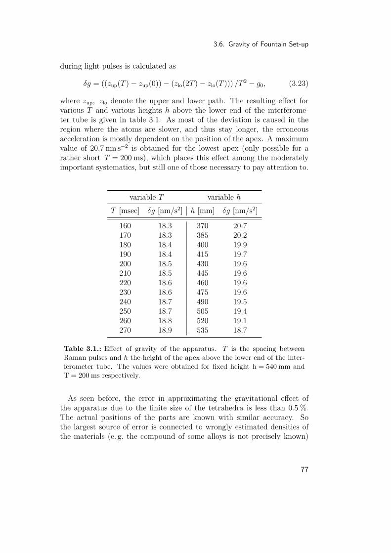
3.6. Gravity of Fountain Set-up
during light pulses is calculated as
δg = ((zup(T )− zup(0))− (zlo(2T )− zlo(T ))) /T 2 − g0, (3.23)
where zup, zlo denote the upper and lower path. The resulting effect forvarious T and various heights h above the lower end of the interferome-ter tube is given in table 3.1. As most of the deviation is caused in theregion where the atoms are slower, and thus stay longer, the erroneousacceleration is mostly dependent on the position of the apex. A maximumvalue of 20.7 nm s−2 is obtained for the lowest apex (only possible for arather short T = 200 ms), which places this effect among the moderatelyimportant systematics, but still one of those necessary to pay attention to.
variable T variable hT [msec] δg [nm/s2] h [mm] δg [nm/s2]
160 18.3 370 20.7170 18.3 385 20.2180 18.4 400 19.9190 18.4 415 19.7200 18.5 430 19.6210 18.5 445 19.6220 18.6 460 19.6230 18.6 475 19.6240 18.7 490 19.5250 18.7 505 19.4260 18.8 520 19.1270 18.9 535 18.7
Table 3.1.: Effect of gravity of the apparatus. T is the spacing betweenRaman pulses and h the height of the apex above the lower end of the inter-ferometer tube. The values were obtained for fixed height h = 540 mm andT = 200 ms respectively.
As seen before, the error in approximating the gravitational effect ofthe apparatus due to the finite size of the tetrahedra is less than 0.5 %.The actual positions of the parts are known with similar accuracy. Sothe largest source of error is connected to wrongly estimated densities ofthe materials (e. g. the compound of some alloys is not precisely known)
77

3. Experiment
and—most importantly—the uncertain geometry of the commercial parts.While some companies—like VAT, the supplier of the vacuum valves—provide detailed CAD-drawings4, others fail to do so. Namely Varian, themanufacturer of the ion pump, gives only very vague information about thedimensions and materials of their products. While some effort was put intoestimating the geometries and masses of pump body and attached magnetan uncertainty of 10 % still needs to be assumed. For all other parts anerror of 5 % in the density is assigned, which gives an overall uncertaintyof 6 % connected to the values shown in table 3.1.
3.7. LaserThe tool with which the atoms are manipulated, and which ideally wouldalso be the only influence acting on them besides gravity, is the laser lightapplied during the various phases of a single interferometer shot. Thisrequires highly stable and versatile laser sources with tight control overtheir spectral qualities, and the ability to precisely determine when andhow much light is administered. Moreover, the system used to generateand shape the light needs to be mobile and rugged in order to fulfil thespecifications of an instrument for field use.A suitable implementation was developed in the course of the work done
by Malte Schmidt in pursuit of his doctorate and is described in great detailin his thesis [70]. Therefore, only a summary of the main characteristics isgiven in the following section.
3.7.1. OpticsCheap diode laser (Sharp GH0781JA2C), commonly used in optical PCdrives, were chosen as the source of coherent light for their availability,compactness, good modal and reasonable optical properties at wavelengthsclose to the desired 780 nm. They deliver 120 mW of light at currents ofup to 170 mA, with a linewidth around 100 MHz determined by the shortlength of their optical medium of about 250 µm.In order to properly address the atomic resonances and especially to
establish a high-quality phase-lock between the Raman lasers, the spectralqualities of the diodes need considerable improvement. To this end, the
4Some caution seems advisable here. It is not an uncommon practice to deliberatelyinsert errors into publicly available drawings in order to make reverse engineeringmore difficult.
78
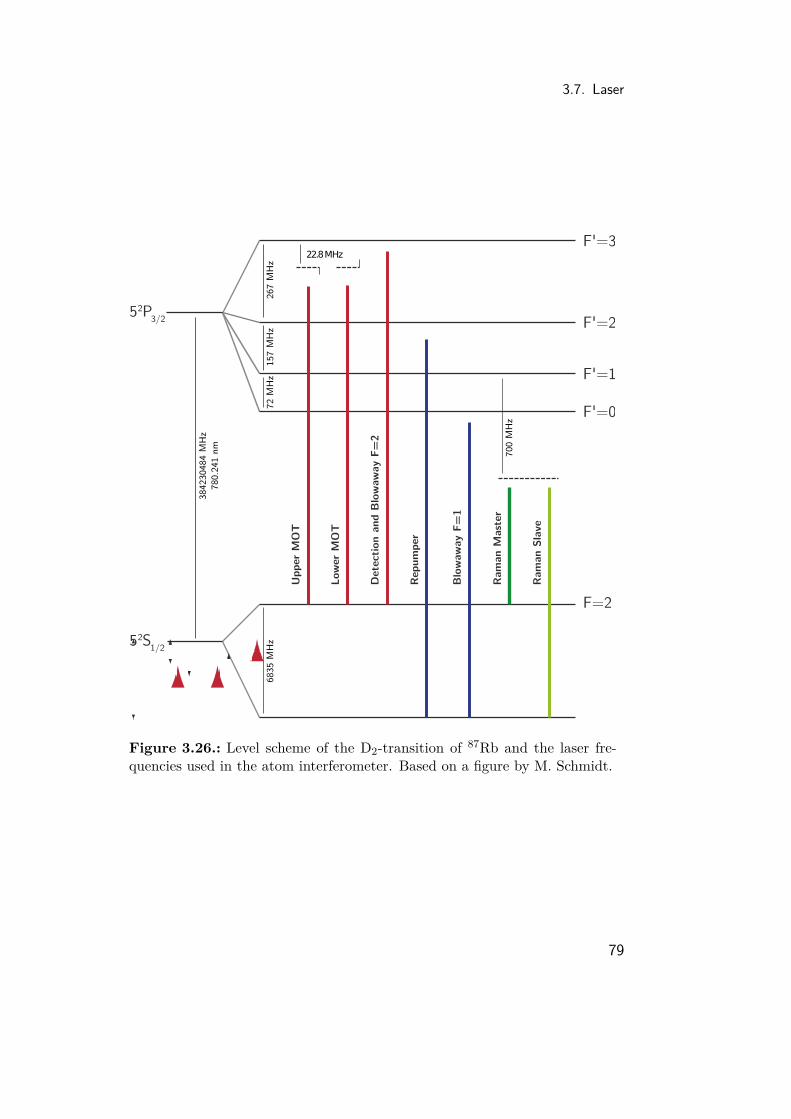
3.7. Laser
52P3/2
52S1/2
Upper
MO
T
Low
er
MO
T
Dete
ctio
n a
nd B
low
aw
ay
F=
2
Repum
per
Blo
waw
ay
F=
1
Ram
an S
lave
Ram
an M
ast
er
F=2
F'=0
F'=1
F'=2
F'=3
700 M
Hz
6835 M
Hz
384230484 M
Hz
7
80.2
41 n
m
72 M
Hz
157 M
Hz
267 M
Hz
Figure 3.26.: Level scheme of the D2-transition of 87Rb and the laser fre-quencies used in the atom interferometer. Based on a figure by M. Schmidt.
79
3. Experiment
diodes are incorporated into an external resonator formed by the backfacet of the diode and an additional piezo-controlled mirror 80 mm apart,brought together in a thermally stabilized block of aluminium. A narrowinterference filter inserted into the light path ensures mono-mode oscillationwith only minimal displacement of the laser beam. This design—dubbedan interference-filter stabilized External-Cavity Diode Laser (ECDL)—wasfirst described in [98] and is highly suitable for very compact and ruggedlaser sources. It is the basic building block of the three distinct lasermodules used in the interferometer.The greater length of the cavity reduces the linewidth to 100 kHz.
By simultaneously adjusting piezo length and diode current a mode-hop-free tuning range of over 9 GHz is achieved, spanning a spectral rangeincluding the D2-resonances of both 85Rb and 87Rb. By modulating thecurrent alone, this range shrinks to 60 MHz but with a possible bandwidthof up to several GHz.One of these improved laser sources is locked to an atomic resonance
by means of Modulation Transfer Spectroscopy [99], where for technicalreasons the F = 3 ↔ F ′ = 4-transition in 85Rb was chosen. Using digitalphase-locks, the other lasers are bound to this reference, which enablesto bridge the substantial frequency gaps between different types of lightused for the experiment (compare figure 3.26). Special emphasis was puton isolating the reference laser from thermal and mechanical disturbancesand on making the spectroscopy lock highly stable.During the MOT and for the beamsplitters several hundred milliwatt
of light are needed. These are generated in a Master-Oscillator-Power-Amplifier (MOPA) configuration where a fraction of the ECDL-light isused to seed a Tapered Amplifier (Eagleyard Photonics). Proper mode-matching allows to draw up to 1 W of light from these semi-conductordevices, from which with some care around 60 % can be fed into an opticalfibre. Two separate pairs of MOPAs are used, one provides the light neededfor cooling, state selection and detection and the other that for the Ramanlasers.Switching and shaping of light pulses is done with AOMs driven by fre-
quencies of 80–200 MHz. This range is conveniently addressed by DirectDigital Synthesis (DDS), a versatile frequency generation technique avail-able pre-packed in dedicated integrated circuits. The technique allows forhighly precise and flexible control over the timing and the frequency of laserlight at different points in the experiment, and is the basis on which thecontrol-system of the experiment is founded (see next section). Voltage-variable attenuators in the rf-paths feeding the AOMs enable fine-grained
80
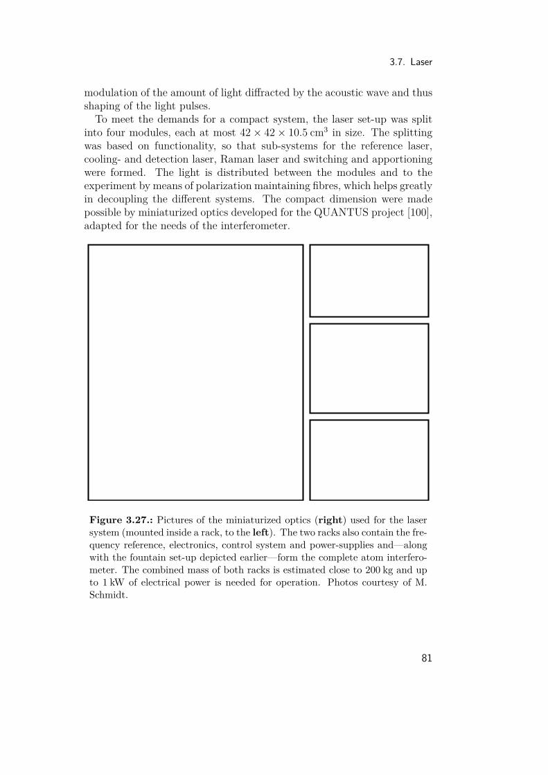
3.7. Laser
modulation of the amount of light diffracted by the acoustic wave and thusshaping of the light pulses.To meet the demands for a compact system, the laser set-up was split
into four modules, each at most 42× 42× 10.5 cm3 in size. The splittingwas based on functionality, so that sub-systems for the reference laser,cooling- and detection laser, Raman laser and switching and apportioningwere formed. The light is distributed between the modules and to theexperiment by means of polarization maintaining fibres, which helps greatlyin decoupling the different systems. The compact dimension were madepossible by miniaturized optics developed for the QUANTUS project [100],adapted for the needs of the interferometer.
Figure 3.27.: Pictures of the miniaturized optics (right) used for the lasersystem (mounted inside a rack, to the left). The two racks also contain the fre-quency reference, electronics, control system and power-supplies and—alongwith the fountain set-up depicted earlier—form the complete atom interfero-meter. The combined mass of both racks is estimated close to 200 kg and upto 1 kW of electrical power is needed for operation. Photos courtesy of M.Schmidt.
81
3. Experiment
3.7.2. Raman Phase Lock
Of crucial importance for the sensitivity and accuracy of the interferometeris the phase-lock between the pair of Raman lasers which drive the matter-wave beamsplitters. Together with Marco Prevedelli from the Università deBologna, an ultra-stable control-loop was developed as described in [101].For this purpose, the light of the two MOPAs in the Raman-module isoverlapped in an optical fibre for spatial mode-cleaning and to preventpointing-instabilities. After the fibre, a small fraction is directed onto afast photodiode, which gives a beat-signal close to the desired splitting of6835 MHz.The beat is mixed down to about 90 MHz and compared to the signal
of a DDS at the same frequency by a low-noise phase-frequency-detector(On Semiconductors MC100EP140). The resulting error signal with a SNRof 121 dB/Hz is fed to a slow conventional PI-controller, which sets diodecurrent and piezo voltage of the slave Raman-ECDL mainly for frequencycompensation, and to a 30 MHz-fast phase-control path, which modulatesthe current of the laser diode directly. By careful tailoring of the circuitrya locking-bandwidth of 4 MHz was achieved, which keeps any detrimentalresonances of the control-loop well above the range of 100 Hz to 60 kHz,where the interferometer is most sensitive to noise in the Raman beams.Consequently, the phase noise spectral density of the closed loop couldbe limited to less than 1 µrad/
√Hz in this band (compare figure 3.28).
Additionally, the high agility of the loop allows to chirp the differencefrequency between the Raman beams in order to compensate for gravityinduced Doppler shifts (required rate ≈ −25.1 MHz/s) by simply alteringthe reference-frequency provided by a DDS.
3.8. Frequency Reference, Timing and Control
The working principle of the interferometer can be summarized as theability of the atoms to very precisely accumulate the phase of the lightfield experienced at three specific points in time. From this picture itbecomes clear that the corresponding frequencies as well as the timing ofthe light pulses have to be known with high accuracy in order to reach thegoals set for the gravimeter.
82

3.8. Frequency Reference, Timing and Control
Figure 3.28.: Phase noise spectral densities of the quartz and that of thefrequency chain used to scale its frequency to 6.8 GHz. Also depicted is thephase noise spectral density of the optical phase lock loop (OPLL) of theRaman lasers. Figure courtesy of M. Schmidt.
3.8.1. Frequency Chain
The basic clock of the experiment is a combination of two ultra-low-noisequartz oscillators: a 5 MHz Wenzel Blue Top to which a 100 MHz WenzelSC Premium is locked in a Spectra Dynamics DLR-100 system. This way,the excellent short-term stability depicted in figure 3.28 is achieved. To pre-vent long-term drifts in the Blue Top, it is bound to a 10 MHz-GPS-signalwith sub-Hertz bandwidth, which in turn profits from the characteristicsof a world-wide network of atomic clocks.To provide all other frequency references used in the interferometer
(mostly 400 MHz for the DDS), as well as the microwave frequencies nec-essary for Raman phase-lock and state-preparation, a frequency chain de-veloped by the group of Arnaud Landragin at SYRTE in Paris [93] is em-ployed. The 100 MHz of the Wenzel SC Premium are doubled and then ex-panded to a harmonic series with multiples of 200 MHz by a comb generator(Picosecond Pulse Labs LPN 7100). Finally a dielectric resonator oscilla-
83

3. Experiment
tor (Raditek RDRO-A-M2-6.8-14d-18V-E-a1) is phase-locked with an offsetof 55.32 MHz provided by a DDS to the 34th harmonic, resulting in the6744.68 MHz necessary for the OPLL discussed above.To assess the limitation to the interferometer’s sensitivity given by the
fluctuations of frequency reference and OPLL, the sum Sφ of the spectralnoise densities given in figure 3.28 weighted with the gravimeter transferfunction is summed, which gives the variance due to Raman phase noise
Var(φRaman) =∞∑n=1|Hφ(2πnfc)|2Sφ(2πnfc) ≈ (6.0mrad√
Hz)2. (3.24)
The uncertainty of 6.0 mrad/√
Hz corresponds to a standard deviationper shot of 6.9 nm s−2, which is well below the noise induced by vibra-tions.
3.8.2. Control of the ExperimentThe operation of the interferometer as a gravimeter is a rather complextask, where a variety of sub-systems need to be actuated with high reliabil-ity and accuracy. All manipulating of the light (shaping and switching oflaser pulses as well as setting the exact phase and frequency) is done withAOMs, which in turn are controlled by DDS and voltage-variable attenu-ators in their rf-path. These again are addressed by voltage signals froma bank of computer-controlled I/O-boards, capable of generating and re-ceiving digital and analogue signals. As these systems are essential for thequality of the gravimeter a short description of the developed techniquesis given in the following sub-section.The DDS used are AD9959 from Analog Devices which provide up
to four independent frequencies. Their phase noise power spectral den-sity at AOM-frequencies around 100 MHz is specified to be better than−134 dBc/Hz for an offset of 1 kHz from the carrier and dropping to−154 dBc/Hz for offsets larger than 1 MHz. Assuming a relevant band-width of 50 MHz for the rf-signal affecting the light in the AOM, thisgives a rms phase error5 of ≤ 200 µrad, which is negligible compared toother noise sources. These numbers hold for a clocking given by an ex-ternal high-quality reference6 of close to 500 MHz fed to the chip directly,avoiding any internal clock multiplier. The DDS feature a frequency tun-
5The conversion from phase noise PSD to phase noise spectral density is simplyL(δf)(dBc/Hz) = Sφ(δf)− 3dB, compare [102].
6Here provided by the frequency chain.
84
3.8. Frequency Reference, Timing and Control
ing resolution of at least 0.12 Hz and 2× 14 bit resolution in phase offsetover a range of 2× 2π, along with the ability to phase-continuously chirpthe frequency with set-able rates. All settings can be programmed to theinternal registers beforehand and triggered with fixed latency by CMOSsignals.The DDS are incorporated in Novatech models 408B and 409B which
provide for additional filtering (smoothing) of the outputs and for pro-gramming of the AD9959 over a RS-232 interface. The 409 features atable mode where the DDS is put through a programmed sequence of fre-quencies and amplitudes of all four channels, while the 408 makes use ofonly one channel as to avoid deteriorating of the signal due to crosstalkbetween outputs. All devices were slightly modified to allow for trigger-ing of the table steps (409) or phase shifts (408) by directly feeding digitalpulses to the Analog Devices chip in order to avoid jitter caused by the No-vatech circuitry. Up to 12 channels of three 409s provide general-purposefrequency signals to address less critical tasks in the laser system, whiletwo 408 are solemnly used to control the frequency chirps and phase shiftsneeded in the Raman phase-lock.Except for programming of the DDS all other parts of the experiment—
mostly shutters in the laser beams and switches and attenuators in the rfpaths—are controlled by precisely timed voltage signals. These are gener-ated by National Instruments I/O-boards (1×DAQ M 6259 and 2×DAQM 6229), with a total of 64 digital and 32 16 bit-wide analogue outputsupdated at a rate of maximal 4 MHz when dedicated channels are used.These cards are housed in a PXI system of the same vendor and controlledby an embedded computer system NI PXI-8196 (Pentium M 2 GHz, 2 GiBRAM) running Windows XP.Developing (2.3) for small time variations δT yields
δφ = keffg2TδT. (3.25)
The effect of jitter—and more importantly—latencies and drifts need tobe limited below the rms-noise per shot and targeted fractional accuracyrespectively. For the more stringent requirement of accuracy this translatesto an uncertainty of
2δTT
< 5× 10⁻¹⁰ (3.26)
which is equivalent to a deviation δT < 57 ps from T = 230 ms. For the jit-ter a much higher limit of 2.3 ns (rms per shot) is valid. While the stabilityof the frequency reference as the basic clock is guaranteed to exceed these
85
3. Experiment
specifications, timing of the Raman laser pulses within these limits is anon-trivial task. This is especially true for a timing system which needs tobe highly versatile and configurable in order to allow for quick adaptationin the course of research and prototyping.To circumvent the notorious timing instabilities of modern PC operat-
ing systems, a scheme was adopted where all triggers are generated by aclock-system fully implemented in hardware. To this end, the I/O-boardsmentioned above are tethered to a trigger pulse generator written intoa Field-Programmable Gate Array (FPGA) (NI PXI7951) housed in thesame PXI system as the controller and I/O-boards. By exploiting thehighly stable trigger lines with fixed latency featured by the PXI system,the digital pulses needed for triggering external events can be generatedwith exceptional stability. This was verified by measuring the differencein arrival time of the raising edge of subsequent TTL-pulses generated byone of the I/O-boards with a Pendulum CNT-90 timer/counter, clockedby the same external reference. The resulting deviations, both randomand directional, from nominal timing were well below 50 ps limited by theresolution of the counter.The desired flexibility is achieved by implementing the trigger pulse gen-
erator with a double counter structure. While one counter is processing alist of points in time at which specified trigger lines are fired to cause theI/O-boards to output the desired voltage signals, the other counter is fedwith a new data-set. Similarly, both the DDSs as well as the I/O-boardsare supplied with new instructions during the 600 ms-long MOT-phase,when all settings of the experiment are static. After the MOT, countersare switched automatically and the timing hardware runs fully autonomousuntil the next MOT-phase, with zero dead-time between shots. This way,stable timing unaffected from OS glitches is ensured, while almost thesame flexibility is obtained as with a system implemented solely in soft-ware.The timing hardware is the lowermost layer in a hierarchically organised
control system. As depicted in figure 3.29, the superordinate layers arewritten in LabView and run parallel to each other in the Windows OS.Communication between different parts is done through FIFOs and a mes-saging system, which ensures a proper sequence of interdependent steps inthe otherwise asynchronous execution. This approach was chosen to allowprompt reaction to user input while being able to guarantee timely repro-gramming of the hardware layer. It is also robust against some temporarilyfailure modes, e. g. denied storage access due to high OS disc activity. Inthis particular case, data to be saved is piled up in the FIFOs until writing
86

3.8. Frequency Reference, Timing and Control
Housekeeping and
Hardware Communication
FPGA NI-DAQ DDShalf-auto-nomuousHardware
MyS
QL
Dat
abas
e
Data ReadoutManagement andAbstraction of Timing
Gravimeter Control
Sof
twar
e (L
abvi
ew)
Use
r In
tera
ctio
n
DataProcessing
Figure 3.29.: The system used to control the experiment is organized inseveral layers. Situated at the bottom is the hardware, which autonomouslyoperates the interferometer during each shot and is only reprogrammed in thestatic MOT phase. With ascending layers, the timing data gets more andmore abstracted and is easily configured by the user through graphical userinterfaces at the top. Data acquisition and storage are parallelized and runpartly on different computer systems.
to the disc is possible again, without impairing the regular cycle of thegravimeter.The middle layer is used for general house-keeping, initializing the other
parts and communication with the timing hardware. The superordinatelayer is responsible for user-interaction and management of the centraldata-structure: a list of time-spans, during which a digital or analoguesignal is to be output through an associated hardware-channel. As thebeginning and end of each pulse can be referenced to other pulses, func-tional blocks in the fountain sequence can be organized. These might shiftin time according to e. g. an extension of the MOT duration, in order toreposition all subsequent steps. This way, a highly flexible description ofthe interferometer cycle is obtained, which allows for easy variation of cer-tain parameters—e. g. height of the apex—without the need to manuallyalter all dependent time-steps.A separate part of the program is dedicated to read and process sensor
input brought in through the digitizers incorporated in the I/O-boards.Most importantly this is the interferometer signal, but also includes tilts,temperatures, residual vibrations on top of the isolation stage and otherenvironmental data which might affect gravimeter performance. This infor-mation is stored in a MySQL-database in human-readable form along with
87

3. Experiment
all details of the sequence for further reference. The interferometer responseis also exposed to other parts of the control system to enable feedback loopsnecessary for the course of the experiment.
3.8.3. Measuring Scheme for GravityFor small phase shifts ∆φ in the interferometer, the fraction of atoms left inthe initial sub-state is described by the simple formula
P(F=2) = 12 (1 + C cos[∆φ+ ∆φ0]) , (3.27)
where C relates to the contrast of the fringe and ∆φ0 describes a potentialphase offset needed in data analysis. Conversely, ∆φ can be fixed within arange of [0, 2π) from the ratio of atoms deduced from the detection signal.This is used to monitor small modulations in g, while the main part isgiven by a linear chirp applied to the reference frequency to which the beatbetween both Raman beams is compared. From the chirp an equivalentphase offset can be calculated as
φ0 = νT (T + 2τ), (3.28)
where ν ≈ −25.1 MHz/s. A factor of 12 is lifted as the chirp shifts both
Raman lasers in opposing directions.As part of an absolute measurement of g, the correct value for ν needs to
be found. This can be done by observing, that for imperfect cancellation ofthe Doppler-shift induced by gravity, the resulting phase can be expressedas
∆φ = (ν − gkeff)T (T + 2τ) (3.29)which, according to equation (3.27), leads to a shift of the observed fringepattern when T is changed. Consequently, the correct chirp rate is found,when the fringe pattern is stationary with respect to a variation of T , asshown in figure 3.30. This is done manually before each long-term gravitymeasurement.After initially obtaining the correct chirp rate, further variations in g
must be kept track of. This is accomplished in the topmost layer of thecontrol system which adjusts chirp rate and Raman phase so as to cancelany observed changes in ∆φ. However some subtleties need to be ad-dressed.From equation (3.27) it is evident, that the interferometer is least suscep-
88

3.8. Frequency Reference, Timing and Control
chirp [MHz/s]
P (F=
2)
0.30.40.50.60.70.8
0.30.40.50.60.70.8
0.30.40.50.60.70.8
0.30.40.50.60.70.8
−25.15290 −25.15285 −25.15280 −25.15275
T = 0.1 s
T = 0.15 s
T = 0.22 s
T = 0.23 s
Figure 3.30.: Fringes obtained by scanning the chirp rate for multiple inter-ferometer timings. Only for the rate which exactly cancels the gravitationalDoppler-shift, the interferometer phase ∆φ becomes independent from varia-tions in T .
tible to small phase changes at the point where ∆φ is cancelled. To regainmaximal sensitivity it is necessary to add and subtract π/2 in subsequentshots to the specific Raman phase which perfectly balances the gravita-tional effect. This results in a pattern where the interferometer "hops" backand forth between the mid-range points of the slopes of the fringe. Whenthe main noise source is independent of the quantum projection noise, afactor
√2 in sensitivity is gained this way, equivalent to the ratio of the
first derivative at the slope to the mean of the derivative over the completecosine. An additional advantage is an increased robustness against varia-tions in the fringe contrast and moderate drifts in a vertical offset, whichotherwise might be interpreted as gravity changes.The overall measurement process is split into several sections. First, a
full fringe is scanned by altering the Raman phase in the second half of theinterferometer sequence in small steps over the course of 72 shots. By fittingequation (3.27) to the obtained series, contrast and central phase ∆φ0 are
89
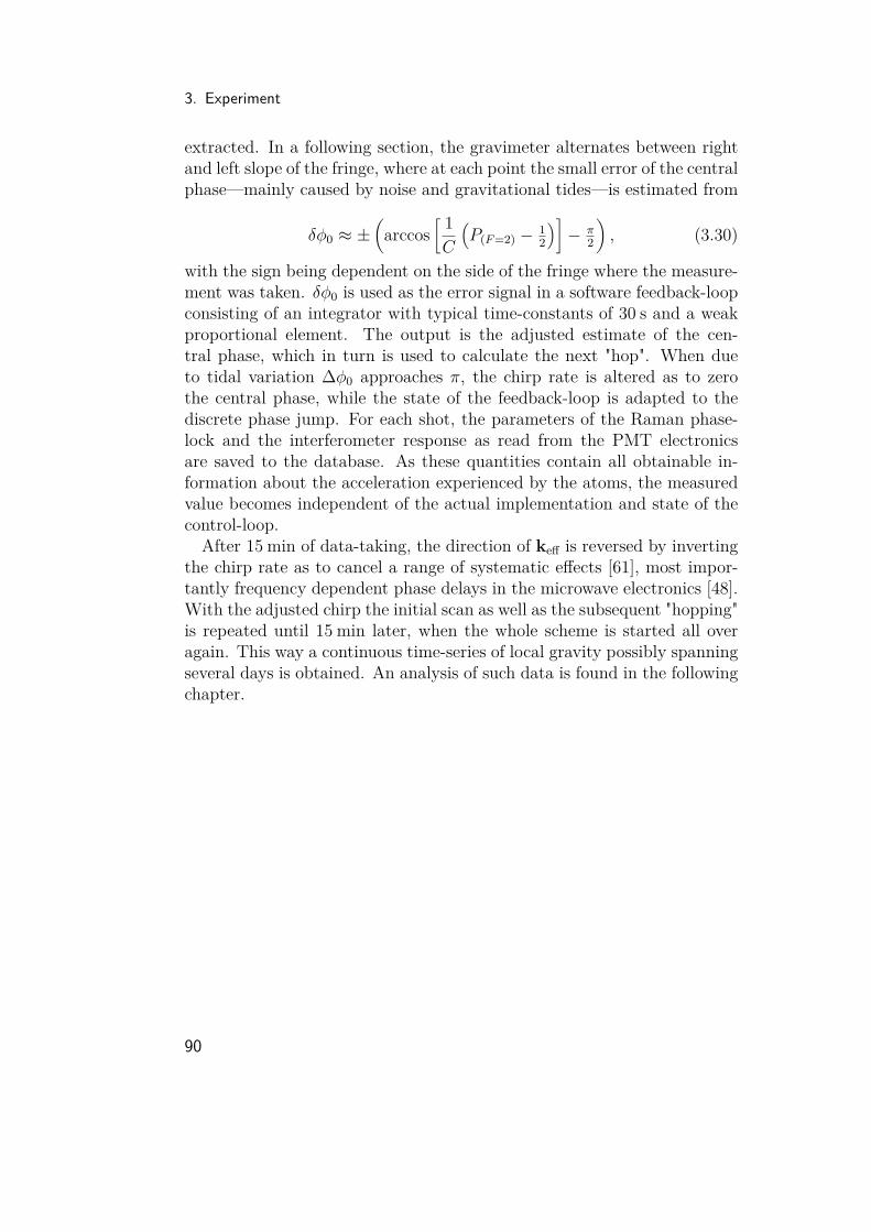
3. Experiment
extracted. In a following section, the gravimeter alternates between rightand left slope of the fringe, where at each point the small error of the centralphase—mainly caused by noise and gravitational tides—is estimated from
δφ0 ≈ ±(
arccos[ 1C
(P(F=2) − 1
2
)]− π
2
), (3.30)
with the sign being dependent on the side of the fringe where the measure-ment was taken. δφ0 is used as the error signal in a software feedback-loopconsisting of an integrator with typical time-constants of 30 s and a weakproportional element. The output is the adjusted estimate of the cen-tral phase, which in turn is used to calculate the next "hop". When dueto tidal variation ∆φ0 approaches π, the chirp rate is altered as to zerothe central phase, while the state of the feedback-loop is adapted to thediscrete phase jump. For each shot, the parameters of the Raman phase-lock and the interferometer response as read from the PMT electronicsare saved to the database. As these quantities contain all obtainable in-formation about the acceleration experienced by the atoms, the measuredvalue becomes independent of the actual implementation and state of thecontrol-loop.After 15 min of data-taking, the direction of keff is reversed by inverting
the chirp rate as to cancel a range of systematic effects [61], most impor-tantly frequency dependent phase delays in the microwave electronics [48].With the adjusted chirp the initial scan as well as the subsequent "hopping"is repeated until 15 min later, when the whole scheme is started all overagain. This way a continuous time-series of local gravity possibly spanningseveral days is obtained. An analysis of such data is found in the followingchapter.
90

4. ResultsWhile the gravimeter is not yet developed to a point where all limiting sys-tematic effects are fully understood, it is nonetheless possible to make high-precision measurements comparable to other state-of-the-art instruments.A valuable evaluation of its characteristics is made possible by comparinggravity data obtained with the atom-interferometer to that from a FG5measured at the same site. This discussion can be found in a later sectionof this chapter, while in a first part noise and the resulting limitations toachievable sensitivity are analysed.
4.1. NoiseAs the cloud of atoms subjected to the interferometer is an incoherent setof quantum systems, the measurement of the occupation of the hyperfineground states suffers from full quantum projection noise [103], which ul-timately limits the achievable SNR in the interferometer signal to 1/
√N ,
where N is the number of atoms.After launch, the cloud consists of roughly 3 × 10⁸ atoms, which are
reduced by a factor of 23 through velocity selection, and another factor of3 by rejecting atoms in the wrong magnetic sub-state. That leaves 4× 10⁶
atoms for detection, from which about 3.5 % are situated in the detection-volume of 8×8×8mm3 due to thermal expansion of the cloud. The resultingnumber of 1.4×10⁵ is equivalent to a SNR of 370. From this ratio a per-shotprecision in the measured interferometer phase of
σproj = C
SNR≈ 1.3mrad (4.1)
can be deduced, where C is again the fringe contrast.However, with the current detection being based on a PMT, this SNR
might be difficult to reach.1 This comes as the noise of photomultiplier1To alleviate the situation an improved detection technique is currently being devel-oped, where the atom number is deduced from the absorption signal found in thedetection laser in comparison to an unaffected beam. This balanced measurementenables rejection of technical noise intrinsic to the laser [104] and should allow for
91
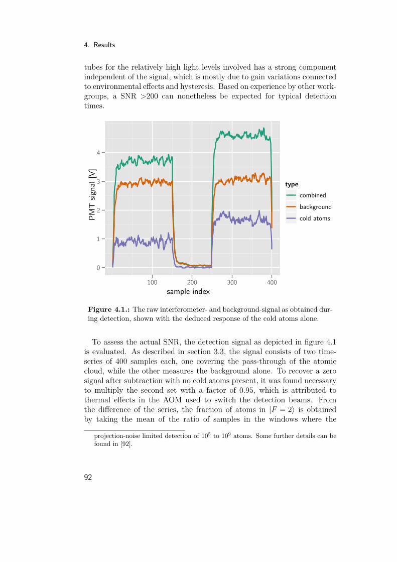
4. Results
tubes for the relatively high light levels involved has a strong componentindependent of the signal, which is mostly due to gain variations connectedto environmental effects and hysteresis. Based on experience by other work-groups, a SNR >200 can nonetheless be expected for typical detectiontimes.
sample index
PMT
signa
l [V]
0
1
2
3
4
100 200 300 400
typecombinedbackgroundcold atoms
Figure 4.1.: The raw interferometer- and background-signal as obtained dur-ing detection, shown with the deduced response of the cold atoms alone.
To assess the actual SNR, the detection signal as depicted in figure 4.1is evaluated. As described in section 3.3, the signal consists of two time-series of 400 samples each, one covering the pass-through of the atomiccloud, while the other measures the background alone. To recover a zerosignal after subtraction with no cold atoms present, it was found necessaryto multiply the second set with a factor of 0.95, which is attributed tothermal effects in the AOM used to switch the detection beams. Fromthe difference of the series, the fraction of atoms in |F = 2〉 is obtainedby taking the mean of the ratio of samples in the windows where the
projection-noise limited detection of 105 to 109 atoms. Some further details can befound in [92].
92

4.1. Noise
fluorescence signal is maximal and flat. For the analysis, the edges of thedetection pulses were trimmed, as these might be susceptible to hysteresiseffects in the PMT.Calculating the standard error of the mean for the raw signal in each
detection pulse, prior to subtraction of the background, yields a fractionaluncertainty of 2.4× 10⁻³, which can be translated to a SNR per detection-pulse of ≈ 400 due to signal-fluctuations alone.2 This is consistent withthe performance expected from a PMT, further supported by the obser-vation that the noise is non-white but shows clear signs of strong low-frequency components, often found in noise generated by technical equip-ment.
counter−propagating beams
phase [rad]0 1 2π π 3 2π 2π
co−propagating beams
phase [rad]
fract
ion
F =
2
0.0
0.2
0.4
0.6
0.8
1.0
0 1 2π π 3 2π 2π
Figure 4.2.: Typical Interferometer fringes obtained with T = 230 ms for thecase of Doppler-insensitive (left) and Doppler-sensitive (right) Raman tran-sitions and fitted cosine. The standard deviation σratio of the residuals plottedbelow is 0.011 and 0.02 respectively, yielding a SNR of 80 and 18.
2It might be puzzling at first, that the obtained SNR is higher than allowed by quantumprojection noise. Here the quantum nature of the system is not a limitation, as itonly concerns the ability to determine the ratio of atoms in different sub-states, notthe quality of the fluorescence signal.
93

4. Results
Computing the ratio of atoms according to the recipe from above com-bines the noise from all pulses and lowers the SNR per shot to about100 (signal amplitude is halved during background elimination, 4 pulsescontribute). This is indeed what can be observed in fringe data (see fig-ure 4.2) when the influence of vibrations is suppressed by employing aDoppler-insensitive scheme, where co-propagating beams drive the Ramantransition. Here the SNR—scaled by the fringe contrast of 80 %—is 80,which allows to identify the PMT-noise as one of the candidates to limitachievable interferometer performance above what is given by quantumprojection noise. When scaled to the contrast of the Doppler-sensitive case,this results in a per-shot precision of the gravimeter
σgrav = σratioCkeffT 2 ≈ 65nm s−2 (4.2)
equivalent to a fractional uncertainty of 6.6 × 10⁻⁹ in g, when measuringat the slope.
4.1.1. Measured NoiseAs can be seen in figure 4.2, in the case of Doppler-sensitive Raman-transitions the noise is roughly doubled. This can best be deduced from acontinuous time-series obtained according to the scheme discussed in theprevious chapter. Depicted in figure 4.3 is the part of one measurement sec-tion (single direction of keff) where the interferometer switches between theslopes of the central fringe. The residuals exhibit mostly white noise andlittle modulation of the averaged value as revealed by the added LOESSsmoother3. The resulting resolution of 160 nm s−2/
√Hz is substantially
better than what can be expected from classical gravimeters (see next sec-tion) and is competitive with recently reported performance of other atominterferometers [59]. However, as the obtainable resolution depends onsite-specific noise a direct comparison with other gravimeters is necessaryin order to fully specify the performance.Further insight is gained from a spectral analysis of the residual accel-
erations in a gravimetric measurement spanning 18 h, which is given in3This method adds a curve by point-wise fitting a simple polynomial to an adjustablespan of the neighbouring data weighted by their distance. Throughout this workpolynomials of degree two and a span of 75 % is used, as implemented as default inthe statistical computing environment R [105]. Here the intention of the smootheris only to ease perception of modulation hidden in the data; therefore further detailsare omitted.
94

4.1. Noise
count
σ = 132 nm s−2
0 20 40 60 80time [s]
res.
acce
lerat
ion
[nm
s−
2 ]
−400
−200
0
200
400
0 200 400 600 800
Figure 4.3.: Typical time-series of gravitational data with only tides and themean subtracted. The depicted standard deviation translates to an equivalentresolution of 158 nm s−2/
√Hz or ∆g
g = 1.6× 10⁻⁸ /√
Hz.
figure 4.4. The data was corrected for tides, polar motion, air pressureand effects connected to the direction of the effective wave vector, whereafter its power spectral density (PSD) was estimated. Please note that nofurther de-trending was necessary to reach the depicted long-term stability.A side-by-side comparison with the PSD obtained from the accelerometersignal on top of the vibration isolation stage shows that the gravimeteris essentially unaffected by environmental noise for frequencies lower than0.1 Hz. The flat noise floor extending to the left is consistent with thestandard deviation found in the time series from figure 4.3, which furthersupports the assumption of white noise in the measurements, caused mainlyby perturbations at higher frequencies. Accordingly, it can be concludedthat the rejection of vibrations by the isolation stage at low frequencies isgood enough to allow for even better performance.The integrated accelerometer noise, weighted with the sensitivity of the
interferometer, reveals that the strong microseisms present close to 0.1 Hzhave a dominant influence on gravimetric noise. As these perturbations
95
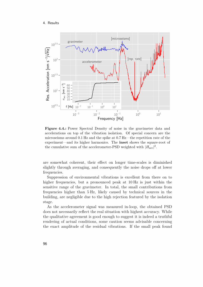
4. Results
Frequency [Hz]
Res.
Acce
lerat
ion
[nm
s−
2Hz
]
100.5
101
101.5
102
102.5gravimeter
accelerometer
[microseisms]
[rep. rate]
10−3 10−2 10−1 100 101
f [Hz]
σac
c. [n
m s−
2 ]
102030405060
10−2 10−1 100 101
Figure 4.4.: Power Spectral Density of noise in the gravimeter data andaccelerations on top of the vibration isolation. Of special concern are themicroseisms around 0.1 Hz and the spike at 0.7 Hz—the repetition rate of theexperiment—and its higher harmonics. The inset shows the square-root ofthe cumulative sum of the accelerometer-PSD weighted with |Hacc|2.
are somewhat coherent, their effect on longer time-scales is diminishedslightly through averaging, and consequently the noise drops off at lowerfrequencies.Suppression of environmental vibrations is excellent from there on to
higher frequencies, but a pronounced peak at 10 Hz is just within thesensitive range of the gravimeter. In total, the small contributions fromfrequencies higher than 5 Hz, likely caused by technical sources in thebuilding, are negligible due to the high rejection featured by the isolationstage.As the accelerometer signal was measured in-loop, the obtained PSD
does not necessarily reflect the real situation with highest accuracy. Whilethe qualitative agreement is good enough to suggest it is indeed a truthfulrendering of actual conditions, some caution seems advisable concerningthe exact amplitude of the residual vibrations. If the small peak found
96
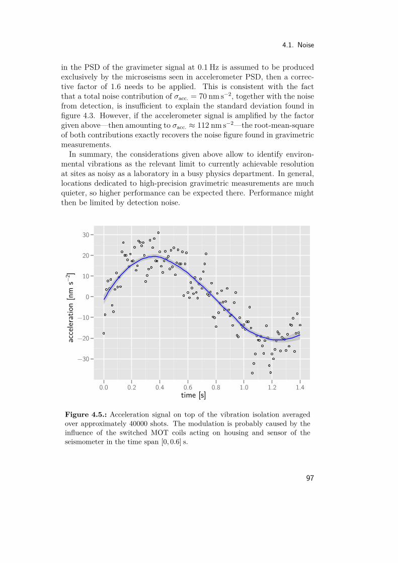
4.1. Noise
in the PSD of the gravimeter signal at 0.1 Hz is assumed to be producedexclusively by the microseisms seen in accelerometer PSD, then a correc-tive factor of 1.6 needs to be applied. This is consistent with the factthat a total noise contribution of σacc. = 70 nm s−2, together with the noisefrom detection, is insufficient to explain the standard deviation found infigure 4.3. However, if the accelerometer signal is amplified by the factorgiven above—then amounting to σacc. ≈ 112 nm s−2—the root-mean-squareof both contributions exactly recovers the noise figure found in gravimetricmeasurements.In summary, the considerations given above allow to identify environ-
mental vibrations as the relevant limit to currently achievable resolutionat sites as noisy as a laboratory in a busy physics department. In general,locations dedicated to high-precision gravimetric measurements are muchquieter, so higher performance can be expected there. Performance mightthen be limited by detection noise.
time [s]
acce
lerat
ion
[nm
s−
2 ]
−30
−20
−10
0
10
20
30
0.0 0.2 0.4 0.6 0.8 1.0 1.2 1.4
Figure 4.5.: Acceleration signal on top of the vibration isolation averagedover approximately 40000 shots. The modulation is probably caused by theinfluence of the switched MOT coils acting on housing and sensor of theseismometer in the time span [0, 0.6] s.
97

4. Results
Another look at the PSD of the accelerometer reveals a disturbing fea-ture at frequencies related to the repetition rate of the experiment and itshigher harmonics. This effect is better approachable in the time domain,when the accelerometer data is cut into segments of the length of one shotsynchronized with the gravimeter sequence. When all pieces are averaged,a signal as depicted in figure 4.5 is found.This disturbance is most likely connected to the switching of the MOT-
coils close to the accelerometer. The effect is probably two-fold: a firstcontribution comes from the accelerations caused by attraction of the steelcontainer housing the accelerometer to the coils, which should mostly berejected by the control loop. A second part can be assumed due to theimpact of the magnetic flux on the sensor inside the accelerometer, causingerroneous acceleration signals, which in turn provoke a reaction of thefeedback loop.As the exact mechanism of the generation of this signal is unclear, as
well as its exact amplitude, a reliable estimation of the necessary correctionof measured gravitation is difficult. In the lack of a better approach, avalue of −10 nm s−2 is assumed, the mean of the depicted signal during thetime interval when the interferometer sequence is applied. However, theproblem should be eliminated in the near future, when a magnetic shield,planned to surround the experiment except for the vibration isolation, isinstalled.
4.2. Gravity measurementIn late November and early December 2010, a first long-term gravimetricmeasurement was carried out at the physics department of the HU Berlin inAdlershof (specific characteristics of the site can be found in appendix A).Data was taken over a period of three weeks, during which some smallertechnical problems concerning the laser, as well as the control system, couldbe identified and lifted, leading to a final measurement starting the fifthof December and spanning 15 hours. The resulting series of gravitationaldata is depicted in figure 4.6. Here, each 15 min-section of data is splitinto 6 points; one from the initial scan over the whole fringe and five fromsubsequent "hopping". The gap around midnight was caused by a laserrunning out of the range of its control loop and subsequent failure of thelock.As can be seen, variations in g as predicted from theory are followed
closely. The solid line given in the top section is the prediction and fitted
98

4.2. Gravity measurement
with an offset as the only free parameter. The result of the fit is theestimate of local gravity and amounts to
g = 9812640796, 2 nm s−2. (4.3)
A closer look at the data points after subtracting these environmentalinfluences reveals a pronounced modulation of the residuals where the signdepends on the direction of the effective wave-vector (up or down) when thedata was taken. This is a systematic effect not yet fully understood, whichneeds further investigation. However, as the perturbation is eminentlysymmetric, high precision in the measurement of g can be recovered byaveraging measurements with anti-parallel wave-vector. To this end, eachpair of consecutive sections with flipping of the wave-vector keff in betweenwere shifted to their common mean by applying
y±i = y±i − (〈y±〉 − 〈y+ ∪ y−〉). (4.4)
Here yi denotes the ith data-point in each section, with the direction of thewave-vector indicated by + and −.After removing the symmetric part of the modulation, the data-points
still show a small residual drift of ≈ 40 nm s−2 over the course of the mea-surement as depicted in the bottom section of figure 4.6. Possible causesfor this perturbation are creep in the tilt-pad in the vibration isolation4,drifts in Raman laser intensity or the frequency reference. The latter ispossible as the GPS-receiver used to stabilize the quartz oscillators on longtime-scales was found to fall clearly behind the specifications given by thevendor. Evaluation of each of these potential sources showed typical driftswhich would result in deviations in measured gravity consistent with theobserved modulation.
Statistical Analysis
The basic approach to retrieve local gravity from the experimental data issimple. In principle the steps described in sub-section 3.8.3 are repeated,that is a cosine is fitted to the scanned fringe according to (3.27) and thefollowing hops are evaluated point-wise using (3.30). An estimate for gis then obtained from evaluating the obtained phase-shifts combined with
4Unfortunately just in the last days of the measurement campaign one of the axes ofthe tilt sensor faulted, thus inhibiting the possibility to correct for small tipping inthe retro-reflector.
99
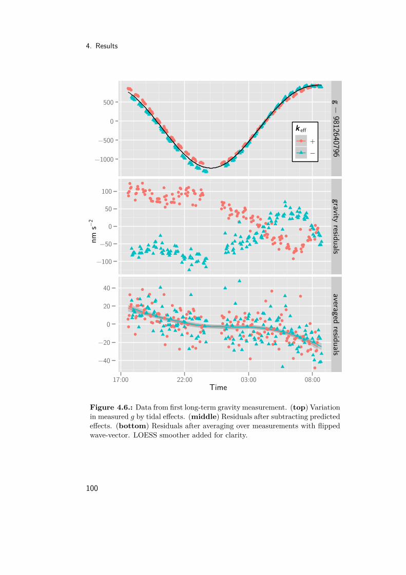
4. Results
Time
nm s−
2
−1000
−500
0
500
−100
−50
0
50
100
−40
−20
0
20
40
17:00 22:00 03:00 08:00
g − 9812640796
gravity residualsaveraged residuals
k eff
+−
Figure 4.6.: Data from first long-term gravity measurement. (top) Variationin measured g by tidal effects. (middle) Residuals after subtracting predictedeffects. (bottom) Residuals after averaging over measurements with flippedwave-vector. LOESS smoother added for clarity.
100
4.2. Gravity measurement
the result from (3.29) with (2.20).While this procedure is trivial enough, a range of purely technical sub-
tleties need to be addressed (e. g. finite frequency resolution of the DDSor robust extraction of atomic ratio from noisy PMT-signal) when pro-cessing the data. Given the high precision of the experiment, even smallmistakes would lead to noticeable changes in the obtained value for g.Therefore, the implementation of the analysis was done independently byfour persons exploiting two different statistical frameworks (Mathematicaand R) and using different approaches (global non-linear fit vs. point-wiseevaluation). Repeated comparison and improvement of the procedure ledto an agreement in the results and associated confidence intervals within1 nm s−2, well within the accuracy limits aimed at with future iterations ofthe experiment.It therefore seems safe to specify the statistical uncertainty down to this
limit. When evaluating the variance of the averaged residuals includingthe observed drift, a standard error of 3.7 nm s−2 is obtained. However,treating the drift as a systematic effect and removing most of the slowmodulation by applying and deducting a linear model, the statistical un-certainty reduces to
σg = 0.8 nm s−2. (4.5)If indeed technical sources can be identified as the cause for this perturba-tion, careful re-evaluation of the analysis procedure is advisable to makefull use of the attainable precision.Some care has been put into the treatment of outliers in the measure-
ment. Occasional glitches in the interferometer lead to < 1 % of shotswhich clearly stand out from the rest of the data.5 To identify such points,a multi-step scheme was adopted. For each 15 min-section of data, a cosinewas fitted to the scanned fringe, and from the residuals those points wereremoved which are farther away than 1.5 times the span between the firstand third quartile from said quartiles. This is similar to a 2σ-criterion as-suming a Gaussian distribution, but less sensitive to distortions caused byextreme outliers [106]. From the remaining points, the standard deviationis calculated, assuming that the variation in the data left is now sufficientlyclose to white noise. Those points in the complete data set (including thepoints initially removed) are then rejected for which the probability to bemeasured given the specified standard deviation is less than a pre-defined
5This figure compares favourably with the performance of classical gravimeters. Inthe absolute measurement done with a FG5 discussed in the following sub-section,1.5 % of the drops needed to be rejected.
101

4. Results
value, typically 0.5 %. The data-set from "hopping" is processed similarly,the only difference being that a simple linear fit is deducted to gather theinitial set of residuals.When comparing the values of g produced from the long data-set from
above with and without cleaning, a deviation of ≈ 0.5 nm s−2 is obtained,which does not grow significantly for stricter thresholds than the 0.5 %noted above. This result demonstrates that careful consideration of outliersis necessary if the high resolution indicated by the variance of data pointswithout drift is to be exploited.
Systematic Influences
While not yet being the subject of a detailed evaluation, some systematicinfluences need to be considered. The two estimated to be the most impor-tant at the moment are the AC Stark and the Coriolis effect.As discussed in section 2.1.1, the shift in ground level energy caused
by a (largely suppressed) coupling to the intermediate level during Ramanpulses can be made equal for both transitions and thus effectively cancelledby choosing an appropriate ratio I23/I13 ≈ 2 of the intensities of the Ramanbeams. However, for some technical reasons the ratio was set to unity,which unfortunately causes a substantial shift in the interferometer phase.As detailed in [70] the erroneous shift can be estimated to cause a deviationin g of −800± 100 nm s−2.Presumably, the most important systematic is connected to the sensitiv-
ity to Coriolis forces of the interferometer. In analogy to light interferome-ter enclosing a finite area between the two arms (Sagnac effect) an atomgravimeter becomes susceptible to rotations if the trajectories of the twowave-packets do not follow the same space-curve. The resulting phase shiftcan be expressed as [107]
∆φsag = 2m~
Ω · A (4.6)
where A denotes the oriented area enclosed by the interferometer and Ωthe angular velocity. In a fountain set-up, the area is due to the recoilsplitting along with small lateral velocity components unavoidable withatomic samples of finite temperature. As there is a broad range of possiblevelocities, the effective area depends on the lateral position difference of thecloud during launch and detection and thus can be reduced by appropriatealignment.For the actual implementation a maximal horizontal deviation of 4 mm
102
4.2. Gravity measurement
is derived from centring the cloud during up- and downward propagationthrough the detection area, leading to vlat = 5.2× 10³ m/s for typical in-terferometer timings. With A = (vlat × ~
mkeff)T 2 the maximal possible
deviation in g can be written as
∆gsag = 2Ωvlat (4.7)
for a given angular velocity. Here Earth’s rotation is of biggest concern,leading to a latitude-dependent rotation rate of Ω⊕ cosα, which for Berlinamounts to 4.4× 10⁻⁵ rad/s. Correspondingly, a maximal error in g of460 nm s−2 is to be expected.In future measurements this can be rectified either by better vertically
aligning launch and detection, averaging over different orientations of theexperiment or actively compensating for Earth’s rotation. The secondmethod is connected to moving the whole apparatus which would intro-duce unwanted tilts. The first method is best implemented by zeroing theeffect of controlled rotations [48]. This necessitates either the ability to ro-tate the fountain set-up—which is impractical—or only the set of Ramanbeams, best done by accurately tilting the corresponding optics. Given thecapability to do the latter, it is also possible to actively compensate for theprecisely known angular motion of Earth during each shot; a method pro-posed by the group of Mark Kasevich in Stanford (USA). As this approachseems to be the most reliable and also the most convenient in field applica-tions, the development of an adequate sub-system is currently under-way.Furthermore fine-tuning of beam verticality becomes straight-forward oncethis functionality is available.
4.2.1. Comparison With FG5Made possible by the kind support of the Bundesamt für Kartographie undGeodäsie, the laboratory in Adlershof could be connected to the gravityreference net in Germany6 in September 2010 [109]. An absolute mea-surement with the FG5 #101 from Micro-g LaCoste Inc. was done in alaboratory on ground floor (room 0’701) in the physics department. Sev-eral other rooms—including 0’703, where the measurement with the atomgravimeter took place—were related to this point with the help of relativegravimeters CG5 from Scintrex Ltd. Furthermore, gravity gradients in allthese places were determined.
6Deutsches Schweregrundnetz 1994 (DSGN 94) [108]
103

4. Results
Figure 4.7.: Pictures taken during absolute gravimetric measurements inlate 2010 at the physics department of the Humboldt Universität zu Berlinwith the atom gravimeter (left) and the FG5 (right).
This enabled the direct comparison of the performance of both gravime-ters. In figure 4.8 the residuals of both measurements after correction fortides are plotted, from which it is apparent that the atom interferometerfeatures a substantially better resolution. Due to the much lower noisefloor, the precision attainable in a given time exceeds that of the FG5 bya factor ≈ 8. This is partly due to the fact, that the corner cube gravi-meter performs a drop every 6 s, and does so for only 15 min every hourin order to preserve the instrument. In contrast, the atom gravimetertakes a data point every 1.4 s, which gives a ratio of ≈ 17 in the effectiverepetition rate, explaining a factor of 4 in the measured noise. Still, theresolution obtained per drop is almost doubled for the atom interferome-ter.As a related note a remark concerning the observed noise level is cited
from [109], which states that due to the vicinity to Berlin a relatively highlevel of microseisms—presumably caused by traffic—is present. This leadsto a standard deviation in measured g values which is 50 % higher thanwhat can be achieved in quieter locations. A similar improvement might
104

4.2. Gravity measurement
Hours since start of measurement
resid
uals
[nm
s−
2 ]
−40
−20
0
20
40
−40
−20
0
20
40
0 2 4 6 8 10 12 14 16 18 20
cold atoms
FG5
Figure 4.8.: Comparison of the residuals from long-term measurements fromatom gravimeter (top) and a state-of-the-art classical instrument (FG5 #101,bottom). Lines are fitted LOESS smoother.
be expected for the atom gravimeter as the observed noise is connectedmostly to residual vibrations.It is also visible from the data that both instruments suffer from si-
milar drifts, with the difference that this effect can much more easily beassessed for the atom interferometer. Indeed, the observed drift has notbeen treated separately in the analysis of the data collected with the FG5by the authors of [109]. Thus the increased resolution will allow for ea-sier characterization of systematic influences, hopefully leading to sizeablegains in performance.To complete the analysis, a comparison of the obtained values for lo-
cal gravity is presented in table 4.1. For convenience, the systematic
105

4. Results
uncertaintyeffect mag. [nm s−2] stat. syst. remarksg (cold atoms) 9812640796 4 7 syst. uncert. mostly
from barometric datagrav. of set-up -19 1MOT switching -10 20AC Stark 800 100verticality 0 220Sagnac 0 460
sum 9812641567 4 520
g (FG5) @ 1.25 m -9812641390 18 15height 403 3 31other room -320 30 94 ±3 cm in floor levelseasons 0 200 estimate from [109]
total 260 36 566
Table 4.1.: Measured values and applied corrections from the comparisonof the atom gravimeter with a FG5. The bottom line is the difference withcorresponding uncertainties.
effects treated in this thesis for which a value can be assigned are in-cluded, despite the lack of importance of some at the current level of ac-curacy.Again, the lower statistical uncertainty for the atom gravimeter is ap-
parent. In contrast, the uncertainty of systematic influences is higher bya factor of 35, underlining the relevance of ongoing efforts to evaluate andsuppress their effects.The value for local gravity obtained with the atom gravimeter agrees
with the one given in the framework of the official German gravity ref-erence net within 260 nm s−2, equivalent to a fraction of 2.3 × 10⁻⁸ in g.The difference is well covered by the combined uncertainty of 570 nm s−2
of the estimated systematics. It can be hoped for that by suppressing thethree most prominent of these effects—AC Stark, verticality and Sagnac,accounting for 92 % of the total uncertainty—a substantial better perfor-mance can be achieved. As a remedy is clearly foreseeable for each of them,fast progress is to be expected.
106

5. Conclusion and Outlook
The atom interferometer described in this thesis is an ongoing effort toimplement the functionality of an absolute gravimeter in a moveable set-uprugged enough for regular deployment in the field, thus pushing matterwaveoptics into the realm of "real world" applications. Albeit development wasstarted from scratch, the performance demonstrated so far exceeds thatof classical instruments by almost an order of magnitude and comparesfavourably with less mobile atom interferometers [48, 59] in respect to theobtainable resolution. This, together with the ability to measure side-by-side with the best available gravimeters at quiet sites, will help greatly inthe oncoming task of identifying and suppressing the influence of systematiceffects.Several steps are scheduled for the near future to address the most im-
portant of the issues encountered recently. These will include in-depthcharacterization of the Raman optics, a magnetic shield encapsulating thecomplete fountain set-up, the ability to remotely control the tilt of theRaman beams with micro-rad resolution, and various improvements tothe laser system (intensity stabilization, lock reliability, thermal regula-tion, better characterization of the master laser). It is anticipated thatthe atom interferometer will then show significantly reduced susceptibilityto external influences and a better control of systematic effects, enablingabsolute gravity measurements competitive with other state-of-the-art in-struments.Future generations of atom gravimeters will certainly aim at vastly re-
duced package sizes. Recent developments in compact interferometer de-signs [110] as well as miniaturized laser systems [111] offer the prospect ofa new class of instruments which deliver the performance of today’s devicesin one hundredth of the volume and smaller, with greatly lowered powerdemands. This will open new fields of applications, where similar systemsare installed as permanent sensors close to geologically active areas, orare part of large-scale precision mapping of gravity in airborne missions.The latter was mentioned being particularly urgent in dialogues with thegeodetic community, as conventional instruments based on spring systemssuffer from lengthy settling times following disturbances frequently found
107
5. Conclusion and Outlook
on low-altitude trajectories. Here, the ability to rapidly prepare and de-ploy a new sample of cold atoms will aid greatly in achieving superioravailability, thereby enabling far better coverage of the area to be investi-gated.A field which will benefit far more than others from miniaturization are
satellite missions aimed at improving geoid reference systems and globalsurveillance. Two projects of the recent past—GRACE and GOCE—havedemonstrated the enormous potential of gravitational mapping from low or-bits and have triggered interest in follow-up missions. Atom interferometershave been proposed as the core sensing technology in such missions, as theypromise better performance in a leaner package. Accordingly, first steps areunder-way to investigate suitable designs [112, 113].The greatly extended times of free evolution possible in micro-gravity will
also serve fundamental research. Tests of the weak equivalence principlecould be carried out with an interferometer very similar to that describedin this thesis, but with two atomic species interrogated at the same time.Differential measurements together with pulse spacings T in the order ofseveral seconds would lead to a strongly enhanced sensitivity to minusculedeviations from the universality of free fall, and could provide for testsorders of magnitude more stringent than the best alternatives availabletoday [114].Another important improvement would be to implement continuous mea-
surements, that is without temporal gaps during shots. This could beachieved by preparing a cloud of atoms while measuring with another, ei-ther in a juggling scheme or by parallel operation of multiple instruments.The benefit would be in avoiding aliasing effects and an extension of thedynamic range of the sensor. With high enough repetition rates to coverall vibrational frequencies of concern, the requirements for vibration iso-lation could be relaxed considerably or avoided all together, allowing forsignificantly reduced complexity of the instrument.The ultimate goal is to combine these aspects in a device capable of
vector measurements of g, that is determination of all three spatial compo-nents of the experienced acceleration in a continuous and robust fashion.As many test masses are available in a cloud of laser cooled atoms, suchmeasurements could happen simultaneously on distinct sets. The compo-nents would need to be separated either spatially through large coherentlytransferred momenta, or in the frequency domain by addressing differ-ent species, isotopes or resonances, in order to distinguish between thethree directions. Instruments able to perform such measurements wouldallow for accurate mapping of gravity independent of orientation on air-
108

borne or seaboard platforms, thus greatly extending the possibilities oftoday.
Figure 5.1.: Today, atom interferometers are still a rare species, seldomlyspotted in the wild.
109

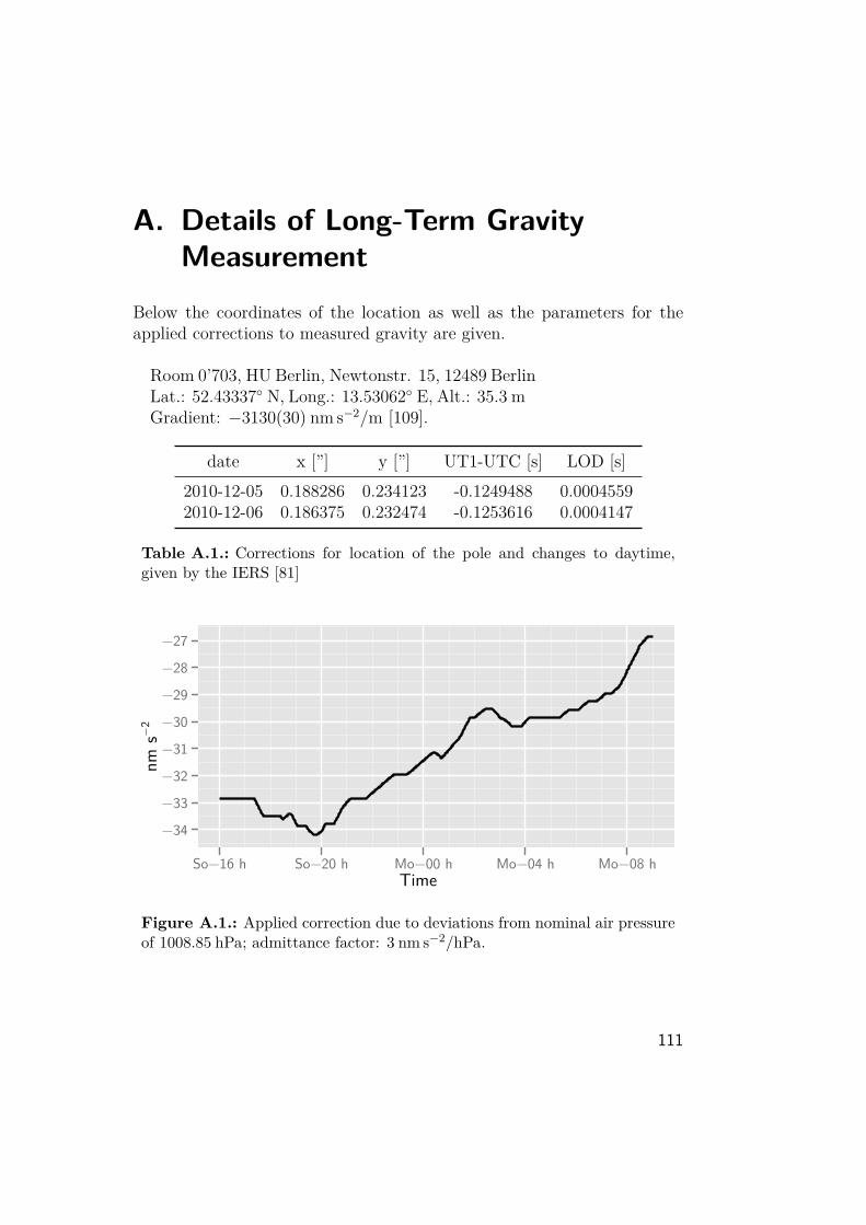
A. Details of Long-Term GravityMeasurement
Below the coordinates of the location as well as the parameters for theapplied corrections to measured gravity are given.
Room 0’703, HU Berlin, Newtonstr. 15, 12489 BerlinLat.: 52.43337 N, Long.: 13.53062 E, Alt.: 35.3 mGradient: −3130(30) nm s−2/m [109].
date x [”] y [”] UT1-UTC [s] LOD [s]2010-12-05 0.188286 0.234123 -0.1249488 0.00045592010-12-06 0.186375 0.232474 -0.1253616 0.0004147
Table A.1.: Corrections for location of the pole and changes to daytime,given by the IERS [81]
Time
nm s−
2
−34
−33
−32
−31
−30
−29
−28
−27
So−16 h So−20 h Mo−00 h Mo−04 h Mo−08 h
Figure A.1.: Applied correction due to deviations from nominal air pressureof 1008.85 hPa; admittance factor: 3 nm s−2/hPa.
111
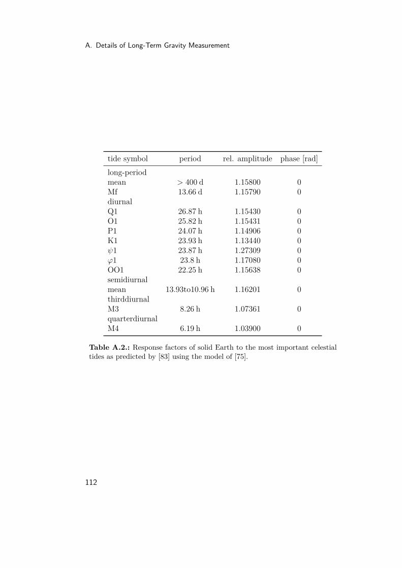
A. Details of Long-Term Gravity Measurement
tide symbol period rel. amplitude phase [rad]long-periodmean > 400 d 1.15800 0Mf 13.66 d 1.15790 0diurnalQ1 26.87 h 1.15430 0O1 25.82 h 1.15431 0P1 24.07 h 1.14906 0K1 23.93 h 1.13440 0ψ1 23.87 h 1.27309 0ϕ1 23.8 h 1.17080 0OO1 22.25 h 1.15638 0semidiurnalmean 13.93to10.96 h 1.16201 0thirddiurnalM3 8.26 h 1.07361 0quarterdiurnalM4 6.19 h 1.03900 0
Table A.2.: Response factors of solid Earth to the most important celestialtides as predicted by [83] using the model of [75].
112

tide symbol period ampl. [nm s−2] phase [rad]long-periodSsa 182.6 d 0.6 -0.059Mm 27.55 d -0.6 -0.358Mf 13.66 d -0.93 -0.482diurnalQ1 26.87 h -0.46 -2.78O1 25.82 h -1.51 2.81P1 24.07 h -0.59 0.94K1 23.93 h -1.83 0.94semidiurnalN2 12.63 h -2.22 1.79M2 12.39 h -9.47 1.34S2 11.97 h -3.49 0.76K2 11.93 h -0.86 0.94
Table A.3.: Effect of ocean loading at the measurement site, provided by [84]
113

B. Aluminium Knife-Edge SealIndustrial standards to achieve UHV-compatible bonding of optical flatsto metal view-ports are brazing and welding, techniques not readily ac-cessible in most laboratories. Custom approaches are mostly based onglueing or "soft" metal seals. The former utilizes chemically hardeningresins, which are conveniently handled, do not introduce any stress ontothe window and can achieve high bake-out-temperatures (> 300 C in [115])for suitable materials. However, they are not in wide-spread use whichseems mostly connected to issues of ageing and cracking under dynamicloads.In contrast, the latter technique benefits from the very forgiving me-
chanical properties many metals exhibit. When put under large enoughcompressive stress, the material starts to become ductile and flows in aform given by the distribution of the load and constraints formed by thegeneral geometry of the surrounding. This way the metal can form anexact counterpart of adjacent surfaces and thus a leak-tight seal. Whenthe stress drops under a certain level—which may happen because themetal deformed to such extent, that the stress-exerting process ran outof energy—a stable situation is regained, where the deformed metal partdoes not alter significantly, if not being objected to stresses similar to thoseexperienced in the first place.1 As metals accept rather large stress beforeplastic deformation happens and as even in such cases they are less sus-ceptible to cracking than e. g. hardened resins, more reliable seals are theresult.The most commonly used metal is indium, due to the peculiar combi-
nation of very low compressive strength of only 2 MPa and low vapourpressure at room temperatures. Indeed, highly reliable UHV-seals of glassto metal are formed with only little pressure needed [96], allowing for thinand brittle windows. Additional benefits are the easy handling2 as well as
1The exact magnitude of stress necessary to induce further deforming is not easilypredictable. This comes as the process is highly non-linear and depends on manyparameters, not the least the kind of metal put under load. Both higher and lowerlimits than before are possible, depending on the alterations to the crystal structureof the deformed part.
2In the cited reference a rather involved procedure is described to obtain the bonding.
115

B. Aluminium Knife-Edge Seal
the glass-wetting property of indium, which leads to strong adhesion andthus further increases the reliability of the seal.Main drawback is the low melting point of 157 C, which puts an incon-
venient limit on bake-out-temperatures. Further points are the compar-atively high price, which might rise significantly in the near future, andthe difficult process of disassembling the window from the viewport, dueto mentioned adhesion. The latter often leads to the loss of the window,further increasing the economic load.
A-A
40,00Ø
Ø30,00
1,40
60° 0,30
0,2 x 45°
Schn
eide Ø 31,00
+0,00 -0.05
A A+
0,05
-0.
002,
00
Figure B.1.: Outer dimensions of and cut through an UHV compatiblewindow-seal made from aluminium. A knife-edge is milled symmetrically toboth sides of an aluminium ring, which is placed between vacuum chamberand window. By applying a large enough load to the window, the edge iscrushed and forms a tight closure with adjacent surfaces.
Several methods have been developed to address these problems. Themost common are to use lead or indium alloys [116] to increase the meltingpoint, or to use a slightly different approach based on knife-edges milled toa ring of copper [117]. Both approaches yield the desired result of raisingachievable bake-out temperatures, but at the price of significantly higherloads to be applied to the seal and consequently to the window. This makesthese techniques error-prone, either by increasing the danger of possibleleaks when being too gentle, or by breaking windows in the attempt toform a reliable connection. However, successful sealing with either method
In practice, very simple methods as pressing the window into a bed of indium aregenerally sufficient.
116
has been demonstrated, albeit accompanied by a pronounced increase inlabour needed in the process.Another potential candidate for the metallic sealant is pure aluminium.
It combines a low price per volume with a sufficiently high melting point of660 C and a yield strength3 of 10− 20 MPa. Copper has a yield strength of≈ 80 MPa in cast form, which drops to ≈ 40 MPa when annealed. Further-more the shear modulus compares as 25.5 GPa for aluminium to 44.7 GPafor copper, and the ultimate strength as ≈ 55 MPa to 220 MPa (annealedcopper). The last quantity gives the highest possible stress on the stress-strain-curve in tension and could be described as the ultimate resistanceof the material to deformation.4While a reliable prediction of the ductile behaviour of the sealant is
impossible from these numbers alone, it becomes apparent, that far lesserstresses will be needed to reach a certain deformation with aluminium thanwith copper. When exploiting the same trick as Noble et al. in [117], thatis to restrain the volume to be deformed to a fine knife-edge as depicted infigure B.1, very low clamping forces are needed.In a test with a window of 40 mm outer diameter and a clear aperture
of ∅30 mm, the torque needed on four M6 screws fixating the window cap(compare figure 3.3) to achieve a nominal reduction in height of 0.6 mmwas < 5 Nm. In comparison, the same torque is needed to compress anindium wire of ∅1 mm to a width of 4 mm in order to form a good seal.For copper a torque three to four times as high was needed. The obtainedseal was helium leak-tested to give an upper bound on the leakage-rate of10−11 hPaL/s, which is sufficient to reach UHV, even if some ten windowsare attached to the vacuum chamber.A problem arises from the pronounced dependency of the mechanical
properties of aluminium on temperature as depicted in figure B.2. If asimple symmetric constellation is chosen as suggested in [117], that is thealuminium ring is paired with a similar one on the opposing side of thewindow covered by the window cap, the increased yielding of the sealantat high bake-out temperatures results in leaks after cool-down. This comesas the energy stored in slight elastic deformations of the window cap isalmost completely used for plastic deformation of the softened aluminium
3Defined as the stress at which plastic deformation begins to occur. As this is not veryprecise for real materials, often (and here) the definition of the stress which leads toa permanent elongation of 0.2 % after removing the load, is adopted.
4The failure mode for tension stress is not necessarily the same as for compression.However, a similar definition for compression loads is not available. To compareboth materials, a regress to this characteristic is necessary.
117
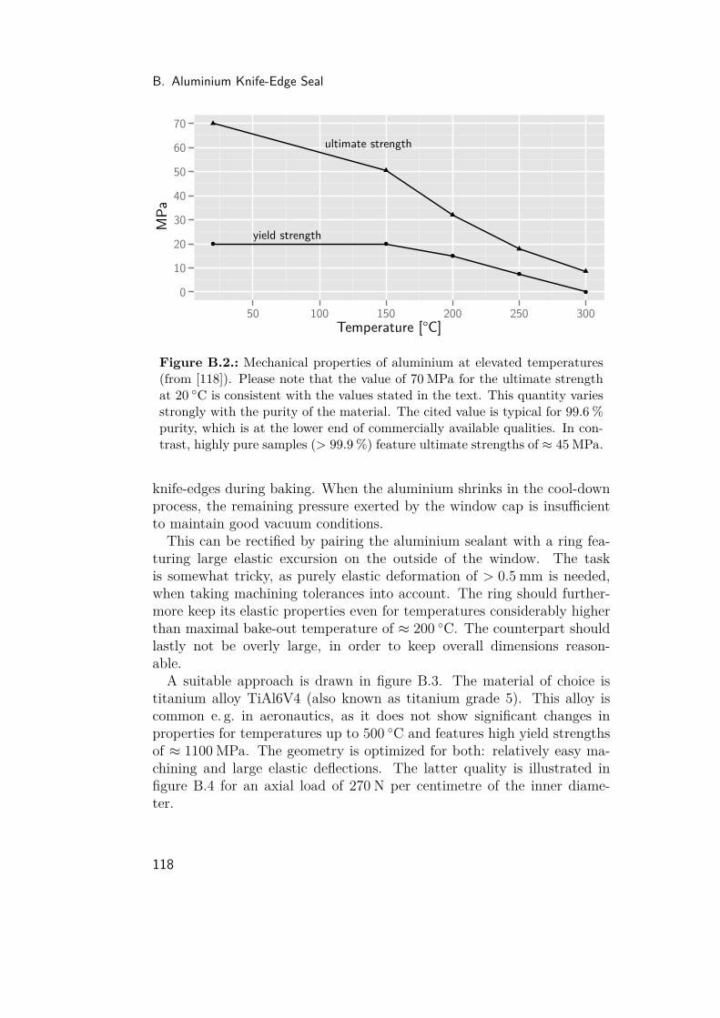
B. Aluminium Knife-Edge Seal
Temperature [°C]
MPa
0
10
20
30
40
50
60
70ultimate strength
yield strength
50 100 150 200 250 300
Figure B.2.: Mechanical properties of aluminium at elevated temperatures(from [118]). Please note that the value of 70 MPa for the ultimate strengthat 20 C is consistent with the values stated in the text. This quantity variesstrongly with the purity of the material. The cited value is typical for 99.6 %purity, which is at the lower end of commercially available qualities. In con-trast, highly pure samples (> 99.9 %) feature ultimate strengths of ≈ 45 MPa.
knife-edges during baking. When the aluminium shrinks in the cool-downprocess, the remaining pressure exerted by the window cap is insufficientto maintain good vacuum conditions.This can be rectified by pairing the aluminium sealant with a ring fea-
turing large elastic excursion on the outside of the window. The taskis somewhat tricky, as purely elastic deformation of > 0.5 mm is needed,when taking machining tolerances into account. The ring should further-more keep its elastic properties even for temperatures considerably higherthan maximal bake-out temperature of ≈ 200 C. The counterpart shouldlastly not be overly large, in order to keep overall dimensions reason-able.A suitable approach is drawn in figure B.3. The material of choice is
titanium alloy TiAl6V4 (also known as titanium grade 5). This alloy iscommon e. g. in aeronautics, as it does not show significant changes inproperties for temperatures up to 500 C and features high yield strengthsof ≈ 1100 MPa. The geometry is optimized for both: relatively easy ma-chining and large elastic deflections. The latter quality is illustrated infigure B.4 for an axial load of 270 N per centimetre of the inner diame-ter.
118
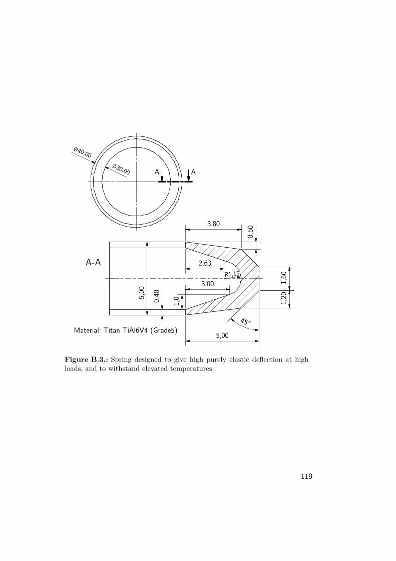
A-A
Material: Titan TiAl6V4 (Grade5)
Ø40,00
Ø30,00
5,00
45°
1,60
5,00
0,40
3,80
0,50
R1,15
3,00
1,0
2,63
1,20
A A
Figure B.3.: Spring designed to give high purely elastic deflection at highloads, and to withstand elevated temperatures.
119
B. Aluminium Knife-Edge Seal
Figure B.4.: Deflection and van-Mises-stress for axial loading (2.5 kN), asobtained from FEM calculations. The uniform colouring of the rims suggests,that the design is fairly optimal. No points with excessive stress are found,which would fail early. Neither are large areas left with significantly lowerstress (except for the inner part, close to the "neutral fibre"), which couldcontribute to further bending if suitably loaded. As the calculated stress iswell below the yield strength, fully elastic behaviour can be expected. Thegrey mesh shows the real (not scaled) deflection.
The height of the window cap is to be chosen so, that when the stackknife-edge-ring–window–elastic ring–window cap is put in its appropriateplace onto the vacuum chamber, an air gap of 1 mm between cap and bodyof the vacuum chamber is left. By simply bolting down the cap to the cham-ber, the knife edge is crushed and the elastic ring is loaded to their nominaldegrees. This procedure does not need to be applied with great care (onlya roughly uniform tightening of the screws to avoid that the window getsjammed inside the cap), as the elastic ring will even out point loads, whichmight otherwise impair the window. After good contact between cap andchamber is established, all screws can be firmly tightened. This way, thewindow cap is a suitable base for further attachments, without the need toworry about undue loads applied to the window.Following this simple recipe, helium leak-tight seals are obtained, which
were tested to rates below 10−11 hPaL/s before and after rapid bakingcycles (max 200 C, heating and cooling rates of > 40 C/h). No windowbroke during numerous assemblies, and sealing was reliable, if large enoughinitial air gaps were chosen. Still more testing is needed, as only a few fullbaking cycles have been done due to tight schedules.
120
It was learned only during the last tests, that the very low torques neededwith indium wires are sufficient to obtain good seals with the aluminiumknife-edges. However, the elastic ring is designed with higher reserves inmind, exceeding the needed stress by approximately a factor of 3. Ad-justing the air gap so, that only torques of 5 Nm were needed to achievefull contact between cap and supporting flange, indeed resulted in leak-tight closures. However, the deflection of the elastic ring was too smallto guarantee adequate loading even after the baking cycle. Instead, leakrates in the order of 10−8 hPaL/s were observed, which are not acceptable.Future design efforts will aim at lowering the load needed to achieve a de-flection in the elastic ring comparable to the one depicted in figure B.4.This is only a question of suitable reduction of wall thickness and someminor adjustments to the geometry, and should not pose any larger prob-lem.
121


Bibliography[1] T. Hänsch and A. Schalow. Cooling of gases by laser radiation. Optics
Communications, 13(1):68–69, January 1975.
[2] S. Chu, L. Hollberg, J. Bjorkholm, A. Cable, and A. Ashkin. Three-dimensional viscous confinement and cooling of atoms by resonanceradiation pressure. Physical Review Letters, 55(1):48–51, July 1985.
[3] E. Raab, M. Prentiss, A. Cable, S. Chu, and D. Pritchard. Trappingof Neutral Sodium Atoms with Radiation Pressure. Physical ReviewLetters, 59(23):2631–2634, December 1987.
[4] L. de Broglie. Recherches sur la théorie des quanta. Thesis, 1924.
[5] C. Davisson and L. Germer. Diffraction of Electrons by a Crystal ofNickel. Physical Review, 30(6):705–740, December 1927.
[6] E. Rupp. Versuche über Elektronenbeugung am optischen Gitter.Die Naturwissenschaften, 16(33):656–656, August 1928.
[7] W. Zinn. Diffraction of Neutrons by a Single Crystal. Physical Re-view, 71(11):752–757, June 1947.
[8] I. Estermann and O. Stern. Beugung von Molekularstrahlen.Zeitschrift für Physik, 61(1-2):95–125, January 1930.
[9] I. Estermann and O. Stern. Beugung von Molekularstrahlen.Zeitschrift für Physik, 61(1-2):95–125, January 1930.
[10] M. Chapman, C. Ekstrom, T. Hammond, R. Rubenstein, J. Schmied-mayer, S. Wehinger, and D. Pritchard. Optics and Interferometrywith Na2 Molecules. Physical Review Letters, 74(24):4783–4786, June1995.
[11] M. Arndt, O. Nairz, J. Vos-Andreae, C. Keller, G. van der Zouw,and A. Zeilinger. Wave–particle duality of C60 molecules. Nature,401(6754):680–682, October 1999.
123

Bibliography
[12] S. Gerlich, S. Eibenberger, M. Tomandl, S. Nimmrichter, K. Horn-berger, P. Fagan, J. Tüxen, M. Mayor, and M. Arndt. Quantuminterference of large organic molecules. Nature Communications, 2:263, March 2011.
[13] L. Marton. Electron Interferometer. Physical Review, 85(6):1057–1058, March 1952.
[14] H. Rauch, W. Treimer, and U. Bonse. Test of a single crystal neutroninterferometer. Physics Letters A, 47(5):369–371, 1974.
[15] M. Kasevich and S. Chu. Atomic interferometry using stimulated Ra-man transitions. Physical Review Letters, 67(2):181–184, July 1991.
[16] F. Riehle, T. Kisters, A. Witte, and J. Helmcke. Optical Ramseyspectroscopy in a rotating frame: Sagnac effect in a matter-waveinterferometer. Physical Review Letters, 67(2):177–180, July 1991.
[17] O. Carnal and J. Mlynek. Young’s double-slit experiment with atoms:A simple atom interferometer. Physical Review Letters, 66(21):2689–2692, May 1991.
[18] D. Keith, C. Ekstrom, Q. Turchette, and D. Pritchard. An interfero-meter for atoms. Physical Review Letters, 66(21):2693–2696, May1991.
[19] A. Cronin, J. Schmiedmayer, and D. Pritchard. Optics and interfer-ometry with atoms and molecules. Reviews of Modern Physics, 81(3):1051–1129, July 2009.
[20] C. Bordé. Atomic interferometry with internal state labelling.Physics Letters A, 140(1-2):10–12, September 1989.
[21] M. Chapman, T. Hammond, A. Lenef, J. Schmiedmayer, R. Ruben-stein, E. Smith, and D. Pritchard. Photon Scattering from Atomsin an Atom Interferometer: Coherence Lost and Regained. PhysicalReview Letters, 75(21):3783–3787, November 1995.
[22] L. Hackermüller, K. Hornberger, B. Brezger, A. Zeilinger, andM. Arndt. Decoherence of matter waves by thermal emission of ra-diation. Nature, 427(6976):711–4, February 2004.
124

Bibliography
[23] K. Zeiske, G. Zinner, F. Riehle, and J. Helmcke. Atom interferometryin a static electric field: Measurement of the Aharonov-Casher phase.Applied Physics B Laser and Optics, 60(2-3):205–209, 1995.
[24] C. Webb, R. Godun, G. Summy, M. Oberthaler, P. Featonby, C. Foot,and K. Burnett. Measurement of Berry’s phase using an atom inter-ferometer. Physical Review A, 60(3):R1783–R1786, September 1999.
[25] C. Ekstrom, J. Schmiedmayer, M. Chapman, T. Hammond, andD. Pritchard. Measurement of the electric polarizability of sodiumwith an atom interferometer. Physical Review A, 51(5):3883–3888,May 1995.
[26] A. Morinaga, T. Tako, and N. Ito. Sensitive measurement of phaseshifts due to the ac Stark effect in a Ca optical Ramsey interferome-ter. Physical Review A, 48(2):1364–1368, August 1993.
[27] C. Degenhardt, H. Stoehr, U. Sterr, F. Riehle, and C. Lisdat.Wavelength-dependent ac Stark shift of the 1S0 −3 P1 transition at657nm in Ca. Physical Review A, 70(2), August 2004.
[28] V. Druzhinina and M. DeKieviet. Experimental Observation ofQuantum Reflection far from Threshold. Physical Review Letters,91(19), November 2003.
[29] J. Perreault and A. Cronin. Observation of Atom Wave Phase ShiftsInduced by Van Der Waals Atom-Surface Interactions. Physical Re-view Letters, 95(13), September 2005.
[30] A. Wicht, J. Hensley, E. Sarajlic, and S. Chu. A Preliminary Mea-surement of the Fine Structure Constant Based on Atom Interferom-etry. Physica Scripta, T102(1):82, 2002.
[31] P. Cladé, E. de Mirandes, M. Cadoret, S. Guellati-Khélifa,C. Schwob, F. Nez, L. Julien, and F. Biraben. Precise measure-ment of h/mRb using Bloch oscillations in a vertical optical lattice:Determination of the fine-structure constant. Physical Review A, 74(5), November 2006.
[32] S. Fray, C. Diez, T. Hänsch, and M. Weitz. Atomic Interferome-ter with Amplitude Gratings of Light and Its Applications to AtomBased Tests of the Equivalence Principle. Physical Review Letters,93(24), December 2004.
125

Bibliography
[33] A. Kellerbauer, M. Amoretti, A. Belov, G. Bonomi, I. Boscolo,R. Brusa, M. Buchner, V. Byakov, L. Cabaret, and C. Canali. Pro-posed antimatter gravity measurement with an antihydrogen beam.Nuclear Instruments and Methods in Physics Research Section B:Beam Interactions with Materials and Atoms, 266(3):351–356, Febru-ary 2008.
[34] T. Heupel, M. Mei, M. Niering, B. Gross, M. Weitz, T. Hänsch, andC. Bordé. Hydrogen atom interferometer with short light pulses.Europhysics Letters (EPL), 57(2):158–163, January 2002.
[35] S. Dimopoulos, P. Graham, J. Hogan, and M. Kasevich. Generalrelativistic effects in atom interferometry. Physical Review D, 78(4),August 2008.
[36] C. Jentsch, T. Müller, E. M. Rasel, and W. Ertmer. HYPER: ASatellite Mission in Fundamental Physics Based on High PrecisionAtom Interferometry, 2004.
[37] S. Dimopoulos, P. Graham, J. Hogan, M. Kasevich, and S. Ra-jendran. Gravitational wave detection with atom interferometry.Physics Letters B, 678(1):37–40, July 2009.
[38] A. Peters, K.-Y. Chung, and S. Chu. Measurement of gravitationalacceleration by dropping atoms. Nature, 400(6747):849–852, August1999.
[39] H. Müller, A. Peters, and S. Chu. A precision measurement of thegravitational redshift by the interference of matter waves. Nature,463(7283):926–9, February 2010.
[40] J. Hammond and J. Faller. Results of Absolute Gravity Determina-tions at a Number of Different Sites. Journal of Geophysical Research,76(32):7850–7854, 1971.
[41] M. Zumberge, R. Rinker, and J. Faller. A Portable Apparatus forAbsolute Measurements of the Earth’s Gravity. Metrologia, 18(3):145–152, July 1982.
[42] R. Colella, A. Overhauser, and S. Werner. Observation of Gravita-tionally Induced Quantum Interference. Physical Review Letters, 34(23):1472–1474, June 1975.
126

Bibliography
[43] T. Gustavson, A. Landragin, and M. Kasevich. Rotation sensingwith a dual atom-interferometer Sagnac gyroscope. CLASSICALAND QUANTUM GRAVITY, 17(12):2385–2398, 2000.
[44] J. McGuirk, G. Foster, J. Fixler, M. Snadden, and M. Kasevich. Sen-sitive absolute-gravity gradiometry using atom interferometry. Phys-ical Review A, 65(3), February 2002.
[45] C. Jekeli. Precision Free-Inertial Navigation with Gravity Compen-sation by an Onboard Gradiometer. Journal of Guidance, Control,and Dynamics, 29(3):704–713, May 2006.
[46] J. Fixler, G. Foster, J. McGuirk, and M. Kasevich. Atom interfero-meter measurement of the newtonian constant of gravity. Science(New York, N.Y.), 315(5808):74–7, January 2007.
[47] G. Lamporesi, A. Bertoldi, L. Cacciapuoti, M. Prevedelli, andG. Tino. Determination of the Newtonian Gravitational ConstantUsing Atom Interferometry. Physical Review Letters, 100(5), Febru-ary 2008.
[48] A. Peters, K.-Y. Chung, and S. Chu. High-precision gravity measure-ments using atom interferometry. Metrologia, 38(1):25–61, February2001.
[49] I. Marson and J. Faller. g-the acceleration of gravity: its measure-ment and its importance. Journal of Physics E: Scientific Instru-ments, 19(1):23–32, January 1986.
[50] G. Geneves, P. Gournay, A. Gosset, M. Lecollinet, F. Villar, P. Pinot,P. Juncar, A. Clairon, A. Landragin, D. Holleville, F. Pereira DosSantos, J. David, M. Besbes, F. Alves, L. Chassagne, and S. Topcu.The BNM Watt Balance Project. IEEE Transactions on Instrumen-tation and Measurement, 54(2):850–853, April 2005.
[51] J. Goodkind. The superconducting gravimeter. Review of ScientificInstruments, 70(11):4131, 1999.
[52] R. Rummel. Dedicated gravity field missions—principles and aims.Journal of Geodynamics, 33(1-2):3–20, March 2002.
[53] M. Ekman and J. Mäkinen. Recent postglacial rebound, gravitychange and mantle flow in Fennoscandia. Geophysical Journal Inter-national, 126(1):229–234, July 1996.
127
Bibliography
[54] G Berrino. Combined gravimetry in the observation of volcanic pro-cesses in Southern Italy. Journal of Geodynamics, 30(3):371–388,February 2000.
[55] G. Budetta and D. Carbone. Potential application of the ScintrexCG-3M gravimeter for monitoring volcanic activity: results of fieldtrials on Mt. Etna, Sicily. Journal of Volcanology and GeothermalResearch, 76(3-4):199–214, April 1997.
[56] J. Faller. Results of an Absolute Determination of the Acceleration ofGravity. Journal of Geophysical Research, 70(16):4035–4038, 1965.
[57] T. Niebauer, D. Sasagawa, J. Faller, R. Hilt, and F. Klopping. A newgeneration of absolute gravimeters. METROLOGIA, 32(3):159–180,1995.
[58] L. Vitushkin, M. Becker, Z. Jiang, O. Francis, T. van Dam, J. Faller,J.-M. Chartier, M. Amalvict, S. Bonvalot, N. Debeglia, S. Deso-gus, M. Diament, F. Dupont, R. Falk, G. Gabalda, C. Gagnon,T. Gattacceca, A. Germak, J. Hinderer, O. Jamet, G. Jeffries,R. Käker, A. Kopaev, J. Liard, A. Lindau, L. Longuevergne, B. Luck,E. Maderal, J. M Kinen, B. Meurers, S. Mizushima, J. Mrlina,D. Newell, C. Origlia, E. Pujol, A. Reinhold, P. Richard, I. Robin-son, D. Ruess, S. Thies, M. van Camp, M. van Ruymbeke, M. deVillalta Compagni, and S. Williams. Results of the Sixth Interna-tional Comparison of Absolute Gravimeters, ICAG-2001. Metrologia,39(5):407–424, October 2002.
[59] S. Merlet, Q. Bodart, N. Malossi, A. Landragin, F. Pereira Dos San-tos, O. Gitlein, and L. Timmen. Comparison between two mobile ab-solute gravimeters: optical versus atomic interferometers. Metrologia,47(4):L9–L11, August 2010.
[60] K. Moler, D. Weiss, M. Kasevich, and S. Chu. Theoretical analysisof velocity-selective Raman transitions. Physical Review A, 45(1):342–348, January 1992.
[61] D. Weiss, B. Young, and S. Chu. Precision measurement of h/mCsbased on photon recoil using laser-cooled atoms and atomic inter-ferometry. Applied Physics B Lasers and Optics, 59(3):217–256,September 1994.
128
Bibliography
[62] C. Bordé and C. Lämmerzahl. Atomic interferometry as two-levelparticle scattering by a periodic potential. Annalen der Physik, 8(1):83–110, January 1999.
[63] C. Bordé. Quantum Theory of Atom-Wave Beam Splitters and Appli-cation to Multidimensional Atomic Gravito-Inertial Sensors. GeneralRelativity and Gravitation, 36(3):475–502, March 2004.
[64] P. Berman, editor. Atom interferometry. Academic Press, 1997.ISBN 978-0-12-092460-8.
[65] C. Bordé. Outils théoriques pour l’optique et l’interférométrie atom-iques. Comptes Rendus de l’Académie des Sciences - Series IV -Physics, 2(3):509–530, April 2001.
[66] C. Antoine. Exact phase shifts for atom interferometry. PhysicsLetters A, 306(5-6):277–284, January 2003.
[67] B. Dubetsky and M. Kasevich. Atom interferometer as a selectivesensor of rotation or gravity. Physical Review A, 74(2), August 2006.
[68] M. Kasevich and S. Chu. Measurement of the gravitational accel-eration of an atom with a light-pulse atom interferometer. AppliedPhysics B Photophysics and Laser Chemistry, 54(5):321–332, May1992.
[69] J. McGuirk, M. Snadden, and M. Kasevich. Large Area Light-PulseAtom Interferometry. Physical Review Letters, 85(21):4498–4501,November 2000.
[70] M. Schmidt. Design, characterization and operation of a mobile high-precision atom interferometer for the measurement of local gravityacceleration. Dissertation, Humboldt-Universität zu Berlin, 2011.
[71] C. Lämmerzahl and C. Bordé. Rabi oscillations in gravitational fields:Exact solution. Physics Letters A, 203(2-3):59–67, July 1995.
[72] C. Antoine. Matter wave beam splitters in gravito-inertial and trap-ping potentials: generalized ttt scheme for atom interferometry. Ap-plied Physics B, 84(4):585–597, July 2006.
[73] P. Storey and C. Cohen-Tannoudji. The Feynman path integral ap-proach to atomic interferometry. A tutorial. Journal de Physique II,4(11):1999–2027, November 1994.
129
Bibliography
[74] P. Cheinet, B. Canuel, F. Pereira Dos Santos, A. Gauguet, F. Yver-Leduc, and A. Landragin. Measurement of the Sensitivity Functionin a Time-Domain Atomic Interferometer. IEEE Transactions onInstrumentation and Measurement, 57(6):1141–1148, 2008.
[75] V. Dehant, P. Defraigne, and J. Wahr. Tides for a convective Earth.Journal of Geophysical Research, 104(B1):1035–1058, 1999.
[76] F. Lyard, F. Lefevre, T. Letellier, and O. Francis. Modelling theglobal ocean tides: modern insights from FES2004. Ocean Dynamics,56(5-6):394–415, September 2006.
[77] J. Merriam. An ephemeris for gravity tide predictions at the nanogallevel. Geophysical Journal International, 108(2):415–422, February1992.
[78] W. Torge. Geodäsie. Walter de Gruyter GmbH & Co. KG, 10785Berlin, 2 edition, 2003. ISBN 3-11-017545-2.
[79] A. Albertella, F. Migliaccio, and F. Sansó. GOCE: The Earth GravityField by Space Gradiometry. Celestial Mechanics and DynamicalAstronomy, 83(1):1–15–15, 2002.
[80] T. Hartmann and H.-G. Wenzel. The HW95 tidal potential catalogue.Geophysical Research Letters, 22(24):3553, 1995.
[81] J. Vondrák and B. Richter. International Earth Rotation and Refer-ence Systems Service (IERS) web: www.iers.org. Journal of Geodesy,77(10-11):585–678, April 2004.
[82] J. Merriam. Atmospheric pressure and gravity. Geophysical JournalInternational, 109(3):488–500, June 1992.
[83] M. Vancamp and P. Vauterin. Tsoft: graphical and interactive soft-ware for the analysis of time series and Earth tides. Computers &Geosciences, 31(5):631–640, June 2005.
[84] M. Bos and H.-G. Scherneck. Ocean tide loading provider. http://froste.oso.chalmers.se/loading//index.html. last visited2011-05-29.
[85] A. Peters. High Precision Gravity Measurements Using Atom Inter-ferometry. Phd thesis, Stanford University, 1998.
130

Bibliography
[86] J. Fils, F. Leduc, P. Bouyer, D. Holleville, N. Dimarcq, A. Clairon,and A. Landragin. Influence of optical aberrations in an atomic gyro-scope. The European Physical Journal D, 36(3):257–260, September2005.
[87] A. Gauguet, B. Canuel, T. Lévèque, W. Chaibi, and A. Landragin.Characterization and limits of a cold-atom Sagnac interferometer.Physical Review A, 80(6), December 2009.
[88] H. Metcalf and P. van Der Straten. Laser Cooling and Trapping.Springer, corrected edition, 1999. ISBN 978-0387987286.
[89] M. Kasevich, D. Weiss, E. Riis, K. Moler, S. Kasapi, and S. Chu.Atomic velocity selection using stimulated Raman transitions. Phys-ical Review Letters, 66(18):2297–2300, May 1991.
[90] D. Steck. Rubidium 87 D Line Data. http://steck.us/alkalidata.revision 2.1.2, 12 August 2009.
[91] A. Kerman, V. Vuletic, C. Chin, and S. Chu. Beyond optical mo-lasses: 3D raman sideband cooling of atomic cesium to high phase-space density. Physical review letters, 84(3):439–442, January 2000.
[92] C. Freier. Measurement of Local Gravity using Atom Interferometry.Diplomarbeit, Technische Universität Berlin, 2010.
[93] J. Le Gouët, T. Mehlstäubler, J. Kim, S. Merlet, A. Clairon, A. Lan-dragin, and F. Pereira Dos Santos. Limits to the sensitivity of a lownoise compact atomic gravimeter. Applied Physics B, 92(2):133–144,June 2008.
[94] S. Merlet, J. Le Gouët, Q. Bodart, A. Clairon, A. Landragin,F. Pereira Dos Santos, and P. Rouchon. Operating an atom inter-ferometer beyond its linear range. Metrologia, 46(1):87–94, February2009.
[95] J. Hensley, A. Peters, and S. Chu. Active low frequency vertical vi-bration isolation. Review of Scientific Instruments, 70(6):2735, 1999.
[96] H. Saeki. Optical window sealed with indium for ultrahigh vacuum.Vacuum, 39(6):563–564, 1989.
131

Bibliography
[97] C. Geuzaine and J.-F. Remacle. Gmsh: A 3-D finite element meshgenerator with built-in pre- and post-processing facilities. Interna-tional Journal for Numerical Methods in Engineering, 79(11):1309–1331, September 2009.
[98] X. Baillard, A. Gauguet, S. Bize, P. Lemonde, P. Laurent, A. Cla-iron, and P. Rosenbusch. Interference-filter-stabilized external-cavitydiode lasers. Optics Communications, 266(2):609–613, October 2006.
[99] J. Shirley. Modulation transfer processes in optical heterodyne sat-uration spectroscopy. Optics Letters, 7(11):537, November 1982.
[100] T. van Zoest, N. Gaaloul, Y. Singh, H. Ahlers, W. Herr, S. Sei-del, W. Ertmer, E. Rasel, M. Eckart, E. Kajari, S. Arnold,G. Nandi, W. Schleich, R. Walser, A. Vogel, K. Sengstock, K. Bongs,W. Lewoczko-Adamczyk, M. Schiemangk, T. Schuldt, A. Peters,T. Könemann, H. Müntinga, C. Lämmerzahl, H. Dittus, T. Stein-metz, T. Hänsch, and J. Reichel. Bose-Einstein condensation in mi-crogravity. Science (New York, N.Y.), 328(5985):1540–3, June 2010.
[101] M. Schmidt, M. Prevedelli, A. Giorgini, G. Tino, and A. Peters. Aportable laser system for high-precision atom interferometry experi-ments. Applied Physics B, 102(1):11–18, October 2010.
[102] M. Thumm, W. Wiesbeck, and S. Kern. HochfrequenzmesstechnikVerfahren und Messsysteme. Vieweg+Teubner Verlag, Wiesbaden,2. durchges. edition, 1998. ISBN 978-3-519-16360-2.
[103] W. Itano, J. Bergquist, J. Bollinger, J. Gilligan, D. Heinzen,F. Moore, M. Raizen, and D. Wineland. Quantum projection noise:Population fluctuations in two-level systems. Physical Review A, 47(5):3554–3570, May 1993.
[104] P. Hobbs. Ultra-quiet high voltage source. IEEE Transactions onInstrumentation and Measurement, 38(5):1004–1005, 1989.
[105] "R Development Core Team". R: A Language and Environment forStatistical Computing. R Foundation for Statistical Computing, Vi-enna, Austria, 2009. ISBN 3-900051-07-0.
[106] R. McGill, J. Tukey, and W. Larsen. Variations of Box Plots. TheAmerican Statistican, 32(1):12–16, 1978.
132

Bibliography
[107] C. Antoine and C. Bordé. Quantum theory of atomic clocks andgravito-inertial sensors: an update. Journal of Optics B: Quantumand Semiclassical Optics, 5(2):S199–S207, April 2003.
[108] W. Torge, R. Falk, A. Franke, E. Reinhart, B. Richter, M. Sommer,and H. Wilmes. Das Deutsche Schweregrundnetz 1994 (DSGN94)Band I. Deutsche Geodätische Kommission, München, b edition,1999. ISBN 3 7696 8589 X.
[109] A. Reinhold and R. Falk. Absolute und relative Schweremessun-gen in der Humboldt-Universität zu Berlin (Campus Adlershof) vom10.-12.09.2010. Technical report, Bundesamt für Kartographie undGeodäsie, 2011.
[110] Q. Bodart, S. Merlet, N. Malossi, F. Pereira Dos Santos, P. Bouyer,and A. Landragin. A cold atom pyramidal gravimeter with a singlelaser beam. Applied Physics Letters, 96(13):134101, 2010.
[111] S. Spießberger, M. Schiemangk, A. Sahm, A. Wicht, H. Wenzel,A. Peters, G. Erbert, and G. Tränkle. Micro-integrated 1 Watt semi-conductor laser system with a linewidth of 36 kHz. Optics Express,19(8):7077, March 2011.
[112] N. Yu, J. Kohel, J. Kellogg, and L. Maleki. Development of an atom-interferometer gravity gradiometer for gravity measurement fromspace. Applied Physics B, 84(4):647–652, July 2006.
[113] F. Sorrentino, K. Bongs, P. Bouyer, L. Cacciapuoti, M. Angelis,H. Dittus, W. Ertmer, A. Giorgini, J. Hartwig, M. Hauth, S. Her-rmann, M. Inguscio, E. Kajari, T. Könemann, C. Lämmerzahl,A. Landragin, G. Modugno, F. Pereira dos Santos, A. Peters,M. Prevedelli, E. Rasel, W. Schleich, M. Schmidt, A. Senger, K. Sen-gstock, G. Stern, G. Tino, and R. Walser. A Compact Atom In-terferometer for Future Space Missions. Microgravity Science andTechnology, 22(4):551–561, September 2010.
[114] S. Dimopoulos, P. Graham, J. Hogan, and M. Kasevich. Testing Gen-eral Relativity with Atom Interferometry. Physical Review Letters,98(11), March 2007.
[115] C. Muller, M. Barrett, and D. Lowenthal. High-temperature windowseals for VUV experiments. Review of Scientific Instruments, 59(8):1425, 1988.
133
Bibliography
[116] S. Cox, P. Griffin, C. Adams, D. DeMille, and E. Riis. Reusableultrahigh vacuum viewport bakeable to 240 °C. Review of ScientificInstruments, 74(6):3185, 2003.
[117] A. Noble and M. Kasevich. UHV optical window seal to conflat knifeedge. Review of Scientific Instruments, 65(9):3042, 1994.
[118] G. Totten and D. MacKenzie, editors. Handbook of Aluminum, Vol.1: Physical Metallurgy and Processes. CRC Press, 1. edition, 2003.ISBN 978-0824704940.
134
List of Figures
1.1. Mach-Zehnder Type Interferometer with Three Light Pulses 41.2. Development of Precision of Absolute Gravimeters . . . . . 71.3. Gravity Effects and Resolution of Modern Gravimeters . . 12
2.1. Interferometer Sequence Under Influence of Gravity . . . . 152.2. Stimulated Raman Transition . . . . . . . . . . . . . . . . 162.3. Interferometer Sequence With Thick Beamsplitters . . . . 222.4. Interferometer Transferfunctions . . . . . . . . . . . . . . . 292.5. Synthetic Tides . . . . . . . . . . . . . . . . . . . . . . . . 32
3.1. Scheme of Fountain . . . . . . . . . . . . . . . . . . . . . . 343.2. MOT-Chamber . . . . . . . . . . . . . . . . . . . . . . . . 363.3. Cut Through MOT-Chamber . . . . . . . . . . . . . . . . 373.4. Magnetic Sub-Levels Resolved by Raman Pulse . . . . . . 383.5. Vacuum Pivot . . . . . . . . . . . . . . . . . . . . . . . . . 393.6. Flux of Quantization Coil . . . . . . . . . . . . . . . . . . 433.7. Residual Flux in Magnetic Shield . . . . . . . . . . . . . . 453.8. Estimation of Wavefront Error . . . . . . . . . . . . . . . . 493.9. Phase Shift Due to Wavefront Curvature . . . . . . . . . . 503.10. Estimation of Error Due to Scatterer . . . . . . . . . . . . 513.11. Phase Shift Caused by a Diffusive Scatterer . . . . . . . . 523.12. Influence of Gouy Phase . . . . . . . . . . . . . . . . . . . 533.13. Alignment of Raman Beams . . . . . . . . . . . . . . . . . 543.14. Commercial Vibration Isolation . . . . . . . . . . . . . . . 593.15. Hysteresis of Vibration Isolation . . . . . . . . . . . . . . . 603.16. Bode Plots of Vibration Isolation . . . . . . . . . . . . . . 643.17. Vibration Spectra With and Without Active Isolation . . . 653.18. Physics Package . . . . . . . . . . . . . . . . . . . . . . . . 673.19. CAD-Drawing of the Moveable Fountain Set-up. . . . . . . 693.20. Tree Representation of Fountain Apparatus . . . . . . . . 713.21. Meshing of Interferometer Parts . . . . . . . . . . . . . . . 723.22. Convergence of Gravity Estimation . . . . . . . . . . . . . 733.23. Gravitation of Fountain-Apparatus in the Interferometer Zone 74
135

List of Figures
3.24. Most Important Sources of Gravity in the Apparatus . . . 753.25. Effect of Fountain Gravity on Atomic Trajectory . . . . . . 763.26. Laser Frequencies . . . . . . . . . . . . . . . . . . . . . . . 793.27. Optical Systems . . . . . . . . . . . . . . . . . . . . . . . . 813.28. Phase Noise Spectral Densities in the Raman Phase-lock . 833.29. Hierarchy of the Control System . . . . . . . . . . . . . . . 873.30. Fringe Spacing vs. Chirp Rate . . . . . . . . . . . . . . . . 89
4.1. Detection Signal . . . . . . . . . . . . . . . . . . . . . . . . 924.2. Interferometer Fringes . . . . . . . . . . . . . . . . . . . . 934.3. Noise in Gravity Measurement . . . . . . . . . . . . . . . . 954.4. Power Spectral Density of Gravimeter Noise . . . . . . . . 964.5. Average Accelerometer Signal During Measurements . . . . 974.6. First Long-Term Gravity Measurement . . . . . . . . . . . 1004.7. Pictures of FG5 and Atom Gravimeter . . . . . . . . . . . 1044.8. Sensitivity of Cold Atoms Gravimeter vs. FG5 . . . . . . . 105
5.1. Fountain During Transport . . . . . . . . . . . . . . . . . . 109
A.1. Pressure Correction . . . . . . . . . . . . . . . . . . . . . . 111
B.1. Drawing of Knife-Edge Window Seal . . . . . . . . . . . . 116B.2. Aluminium at Elevated Temperatures . . . . . . . . . . . . 118B.3. Elastic Counterpart in Window Seal . . . . . . . . . . . . . 119B.4. Elastic Behaviour of Window Spring . . . . . . . . . . . . 120
136

List of Tables
3.1. Gravity of the Apparatus . . . . . . . . . . . . . . . . . . . 77
4.1. Gravimeter Comparison . . . . . . . . . . . . . . . . . . . 106
A.1. Earth Rotational Parameters . . . . . . . . . . . . . . . . . 111A.2. Solid Earth Tides . . . . . . . . . . . . . . . . . . . . . . . 112A.3. Ocean Loading . . . . . . . . . . . . . . . . . . . . . . . . 113
137


Danksagung
Zu guter Letzt bleibt die angenehme Aufgabe, all jenen zu danken, diedirekt oder indirekt an der Entstehung dieser Dissertation mitgewirkt ha-ben.Der erste Dank gebührt Achim Peters, der diese Arbeit in vielerlei Hin-
sicht ermöglicht und auch betreut hat. Es war zu einem guten Teil sei-ne PhD-Thesis, die dazu geführt hat, dass Materiewellengravimeter heutekurz davor stehen, klassische Absolutmessinstrumente zu übertreffen. Oh-ne seinen enormen Schatz an Erfahrungen und sein Wissen um kleinsteDetails wäre sie in dieser Form sicherlich nicht machbar gewesen. Außer-dem möchte ich ihm an dieser Stelle herzlich dafür danken, dass er esmir ermöglichte, einige Zeit in Stanford in der Gruppe von Steven Chuzu arbeiten, einer der Geburtsstätten der Interferometrie mit kalten Ato-men.Malte Schmidt hat mit mir zusammen das Projekt begonnen und zum
jetzigen Stand gebracht. Wir haben uns Photonen und Atome redlichgeteilt, wobei er als Herr über Licht und Schatten die Nase nach ge-lieferten Stückzahlen deutlich vorne hat: während bisher grob geschätzt1017 Rubidiumatome in die MOT geladen und teilweise im Interferome-ter verwendet wurden, mussten dazu etwa 1023 Photonen gestreut wer-den.Unsere Nachfolger Matthias Hauth und Vladimir Schkolnik sind in den
letzten zwei Jahren dazu gestoßen und haben einen gehörigen Anteil an denerzielten Leistungen. Das Projekt wäre noch nicht so weit, ohne ihre Mithil-fe. Ein besonderes Dankeschön geht an Christian Freier. Seine Diplomarbeitwar ein großer Gewinn, und dass er jetzt als Doktorand weitermacht, lässtauf schnelle weitere Erfolge hoffen. Allen drei gebührt Dank für Korrek-turlesen und Verbesserungsvorschläge. Sebastian Grede muß auch erwähntwerden, er hat in seiner Diplomarbeit die ersten Fundamente der Kontroll-software gelegt.Allen fünf danke ich für die kollegiale Zusammenarbeit und die gemein-
samen Anstrengungen. Ein gutes Team ist immer mehr als die Summe derEinzelteile.Trista Freier war so freundlich, dem Englisch allzu deutsche Eigenheiten
139
List of Tables
auszutreiben. Falls der Leser bis zu diesen Seiten gekommen ist, ohne dasGefühl zu entwickeln, dass es hier um „sä atom interferometa“geht, so istdas ihr Verdienst.Die mechanische Werkstatt und besonders Herr Rausche und Herr Fah-
nauer hatten immer ein offenes Ohr für meine vielen – häufig ungewöhn-lichen – Wünsche und mussten oft Außerordentliches leisten, um ihnengerecht zu werden. Die exzellenten Ergebnisse sind ein wesentlicher Grundfür den Erfolg dieses Gravimeters, die ohne die außergewöhnlich gute Zu-sammenarbeit nicht möglich gewesen wären. Außerdem hat Herr Rauscheden Kontakt zur Werkstatt des DESY in Zeuthen und hier besonders zuHerrn Bandke vermittelt, die hervorragende Arbeit bei den aus dem Vollengefrästen Vakuumkammern geleistet haben.Die Mitarbeiter des Geophysikalischen Forschungsinstituts in Potsdam
und des Bundesamts für Kartographie und Geodäsie haben sich sehr be-müht, uns die ersten Schritten in die Welt der Präzisionsgravimetrie soeinfach wie möglich zu machen. Ein herzlicher Dank geht an Herrn Dr.Wziontek, Herrn Dr. Petrovic, Herrn Dr. Schäfer, Herrn Dr. Falk und HerrnReinhold.Ganz besonders muss und will ich meiner Partnerin Sara danken. Sie hat
in den letzten beiden Jahren der Doktorarbeit und insbesondere währendder Monate, in denen ich die Dissertation schrieb, mir den Rücken frei undzwei kleine Jungs im Zaum gehalten; wahrlich keine leichte Aufgabe. Wennes eine Person gibt, ohne die es ganz und gar nicht gegangen wäre, dannist sie es.Für Ferdinand und Felix gibt es zum Schluss ein dickes Papa-Bussi. Ihr
habt zwar nicht wirklich geholfen, aber ohne Euch hätte es viel wenigerSpaß gemacht.
140

SelbstständigkeitserklärungIch erkläre, dass ich die vorliegende Arbeit selbstständig und nur unterVerwendung der angegebenen Literatur und Hilfsmittel angefertigt habe.
Berlin, den Alexander Senger
141
Copyright © 2022 FDOKUMEN