A Minskyan-Fisherian SFC model for analyzing the linkages of privatefinancial behavior and public debt

Italo Pedrosa†�Antonio Carlos Macedo e Silva†

† Institute of Economics/University of Campinas (UNICAMP), Brazil

Abstract. By means of a stock-flow consistent (SFC) model, we explore the linkages among pri-

vate financial behavior, aggregate demand, and fiscal variables, considering three fiscal regimes:

‘automatic stabilizer’, countercyclical and austerity. The model allows for price change and

path-dependency, which emerges from the incorporation of an investment function that relies

on the ‘pure’ accelerator effect, having two major implications. First, in the short-run, contrac-

tionary shifts in financial conditions cause an increase in public debt ratio unconditionally to

the fiscal regime. Second, steady state norms are ultimately determined by the growth rate,

which in turn depends on short-run developments.

This version: February 10, 2016

�E-mail address for correspondence: italopedrosa@gmail.com.

1 Introduction

A well-known stylized fact of major financial crises is the rapid increase of public debt and a

sharp reduction in private debt (Reinhart and Rogoff, 2010). How financial crisis and fiscal

deterioration are connected? Is the increase in public debt the result of a lenient government

fiscal behavior, so the increase in the public debt/GDP ratio is somehow avoidable by a specific

fiscal regime (e.g., austerity)? Which are the best alternatives in what concerns economic activity

recovery and public debt sustainability itself?

In order to discuss these questions, the paper has two main goals: 1) inspired by Minsky’s

‘Big Government’ (Minsky, 1982, 1986), we explore the effects of private financial decisions in

public deficit and debt. Even though several authors (such as Lerner, Steindl, and Godley) are

concerned with the mutual interactions between private demand and fiscal deficit, there is still

room to improve the comprehension of how public debt behaves dynamically when it affects

(and is affected by) private demand; 2) to analyze the extent to which the fiscal regime affects

that relationship.

To address these points, we develop a Minskyan-Fisherian stock-flow consistent (SFC) model

in which private financial decisions affect (in different ways) agents’ balance sheets, investment

financing, and thus aggregate demand. Namely, we address the influence of lender’s risk in the

effective supply of credit to firms, the impact of households’ portfolio decisions on the ability

of firms to raise new finance by means of equity emissions, and the influence of firms’ decisions

regarding their desired leverage ratio. With prices given by a traditional Phillips curve, we

assess the role of price changes in exacerbating cycle’s downswing by increasing the real value

of liabilities and the burden of debt, consistently with Fisher’s (1933) theory.

In the model, the combination of credit contraction and deflation (or even disinflation) can

lead to a harmful descending spiral, for it may increase debt ratios even if debtors are trying to

liquidate liabilities. This point, first stressed by Fisher (1933), is important to our goals because

the interaction between different fiscal regimes and inflation is bound to affect the public and

private debt ratios, the amplitude of output oscillations and the time for the system to stabilize

after a contractionary shock.

The analysis carried out in this paper has similarities with Skott (2001), Schlicht (2006),

Nakatani and Skott (2007), Palley (2010) and Botta (2013). It is indeed more closely related

to Godley and Lavoie (2007a) and Ryoo and Skott (2013). Godley and Lavoie build a full-

employment model with government consumption as the policy instrument, but assume away

capital accumulation; their model therefore lacks the financial behavior of firms, crucial to our

purposes. Ryoo and Skott deploy a richer financial structure, with capital accumulation, but

assuming full employment and given prices.

A contribution of our model is to provide a framework to jointly analyze the short-term

effects of changes in private financial behavior, endogenous inflation rate and different fiscal

regimes (countercyclical policy, austerity and ‘automatic stabilizers’). To our best knowledge,

combining these elements of Minskyan and Fisherian frameworks in a SFC model to analyze the

impacts on fiscal variables has not been done yet, clearly limiting the assessment of the impact

of different fiscal regimes policies. In particular, the assumption of given prices, adopted by

most previous papers, rules out potential negative feedbacks between debt, falling demand, and

1

deflation, through the increase in the real value of liabilities and the burden of debt.

Besides that, another contribution of the paper is to incorporate into the SFC framework an

investment function that relies on the ‘pure’ accelerator effect, being the model’s growth rate

driven by non-capacity creating autonomous expenditures (Lavoie, 2016) – and not investment.

Similar investment functions have recently been discussed in the literature (see for instance

Freitas and Serrano, 2015; Allain, 2015; Lavoie, 2016) as an alternative (or a complement) to

the canonical post-Kaleckian (Bhaduri and Marglin, 1990) investment function. Furthermore,

as we discuss, this particular investment function, that relies in a Harrodian mechanism (Lavoie,

2016), allows for path-dependency in our framework.

The paper is structured as follows. In section 2 we present our SFC model. We perform

simulations changing central financing parameters in section 3. In section 4, we present our final

remarks in light of Minskyan and Fisherian theories.

2 The SFC model

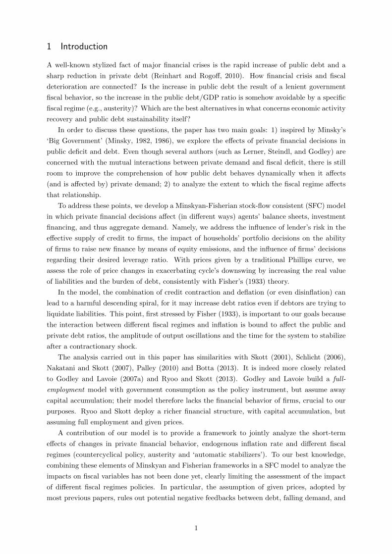
We assume a closed economy, producing a single good, with four sets of agents (households, firms,

banks and government) and five assets (deposits, equities, bills, physical capital and loans). The

accounting framework of the model is described in Table 1, which shows institutional sectors’

balance sheets, and Table 2, providing the transactions and flow of funds matrix.

Stocks of financial variables, shown in Tables 1 and 2, are expressed in nominal values. This

amounts to saying that their price is one, except in the case of the stock prices (pe), which vary

over time. Flow variables presented in capital letters are the real ones. The nominal values can

be obtained by multiplying real variables by p, the general level of prices. Superscripts d and s

stand for demand and supply, respectively. For simplicity, we suppress time subscripts.

Table 1: Institutional sectors’ balance sheets

Households Firms Banks Government∑

1. Deposits +M −M 02. Loans −L +L 03. Fixed capital +pK +pK4. Equity +peE −peE 05. Govt. Bills +B −B 06. Net Worth +V +Vf 0 −B +pK

Government expenditure is G, financed through taxes (T ) and bills (B). The following

equations define government’s constraints and fiscal regimes:

∆B ≡ nB−1 + pG− pT (1)

T = θ

[(1− π)Y + FD + n

M−1 +B−1p

](2)

G = γK−1 (3A)

G = [γ − ε(u− un)]K−1 (3B)

2

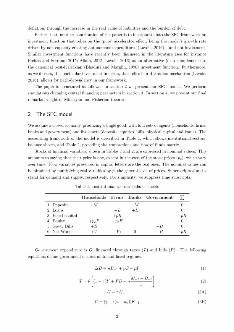
Table 2: Transactions and flow of funds

HouseholdsFirms

Banks Govt.∑

Current Capital

1. Consumption −pC +pC 02. Investment +pI −pI 03. Public Spending +pG −pG 04. Wages +pW −pW 05. Taxes −pT +pT 06. Profits +pFD −pF +pFU 07. Interest on bills +nB−1 −nB−1 08. Interest on loans −nL−1 +nL−1 09. Interest on deposits +nM−1 −nM−1 0

10. Subtotal +SAVh 0 +SAVf +SAVg 0

11. ∆ Deposits −∆M +∆M 012. ∆ Loans +∆L −∆L 013. ∆ Equity −pe∆E +pe∆E 014. ∆ Bills −∆B +∆B 0

15.∑

0 0 0 0 0 0

G =

min[τ1T−1, G−1(1 + τ2)], if ∆b−1 > 0

τ1T−1, otherwise(3C)

where n is the nominal interest rate, exogenously defined by the government, θ is the tax rate

on households income, π is the profit share, Y is the real output, FD is dividends distributed

by firms, M is households deposits, K is the real capital stock, ε gives the intensity of the

adjustment of government expenditure ratio to the activity level, u is the capacity utilization,

un is the normal long run capacity utilization, b = B/pK−1 is the public debt to capital ratio

(we henceforth refer to ratios to capital simply as ratios), γ is a constant defining government

expenditure ratio, τ1 is a constant defining the ratio of government expenditure to the lagged

tax revenues and τ2 is the long-run growth of potential output, which for simplicity we assume

to be the moving average of capital stock growth.1

Equation (1) is the identity defining the government budget constraint: public debt in period

t depends on previous period stock of public debt plus interest, and on the primary deficit

(p.G − p.T ). Equation (2) defines real tax revenue. For simplicity, we assume that the only

source of tax revenue is households’ wages and financial income, and that the (income) tax rate

θ is exogenously defined.

The following three equations define the government expenditure regimes. In the ‘automatic

stabilizer’ case (3A), the government expenditure is a constant fraction γ of capital stock, as

in Dos Santos and Zezza (2008). Notice that, in (3A), when capacity utilization goes down,

government expenditure ratio (G/K−1) is constant over time, but the share of government

expenditure to GDP ratio will increase. In the second case (3B), the government expenditure

1From equation (14), we have that potential output is Yfc = σK−1. Then, as Yfc,−1 = σK−2, it is straightforwardto show that gfc = ∆Yfc/Y−1 = gk,−1

3

ratio varies according to the deviation of capacity utilization from its long-run ‘normal’. This

can be interpreted as a countercyclical fiscal regime. The third government expenditure function

(3C) is the austerity case. When the lagged public debt ratio (b−1) increases, the government

expenditure in the following period will be the minimum of two values: the multiplier τ1 times

lagged tax revenue and the lagged government expenditure multiplied by the long-run growth

of potential output (τ2). When the public debt ratio is not increasing, government expenditures

and tax revenues grow at the same rate. Equation (3C) assures that the government mitigates

(or compensate) the primary deficit gap in the aftermath of any event that increase public debt

ratio.

Households receive wages (W = (1 − π)Y ) and dividends (FD) from firms, interests on

government bills and on bank deposits, and decide how much to consume. Their asset portfolio

is composed of deposits (M), stocks (E) and government bills (B).

C = (1− θ){α1(1− π)Y + α2

[FD + n

M−1 +B−1p

]}+ α3

V−1p

(4)

SAVh = (1− θ)[(1− π)pY + pFD + n(M−1 +B−1)]− pC (5)

V ≡ V−1 + SAVh + ∆peE−1 (6)

Real consumption level is determined by means of a standard consumption function, represented

in equation (4), where α1 is the propensity to consume out of after-tax wages, α2 is the propensity

to consume out of after-tax financial income and α3 is the propensity to consume out of wealth.2

We assume, for simplicity, that α1 = α2 = α. Equation (5) defines households’ nominal savings

(nominal disposable income less nominal consumption). Recalling that stock prices fluctuate,

the household budget constraint requires the inclusion of capital gains, which affects the end-of-

period wealth given in (6). Plugging (4) and (5) into (6) we obtain:

V ≡ (1− α3)V−1 + (1− θ)(1− α)[(1− π)p.Y + p.FD + n(M−1 +B−1)] + ∆peE−1 (7)

In each period, households decide how to allocate wealth. In equation (8), defining the price

of stocks, δ is the share of wealth the households allocate in stocks. This parameter is assumed

to be exogenously given, capturing the current state of expectations. The amount of stocks E

is decided by the firms. Thus, stock prices (pe) clear the market, so that Ed = Es.

Conversely, households demand a share (1 − δ) of interest-bearing securities, which can

be either public bills or bank deposits. As Ryoo and Skott (2013), we assume that bills and

deposits are perfect substitutes, having the same remuneration. An extra hypothesis is attached:

all the bills supplied by the government are demanded by households (9), while deposits are

obtained as a residual, closing the households budget constraint (10). This hypothesis avoids

the indetermination in portfolio allocation (as both assets have the same risk and the same

yield), and also offers a palatable ‘closure’ for the model, which will be pointed latter.

pe =δV

E(8)

B = Bs = Bd (9)

2In our model wealth is equal to net wealth, as households are assumed to have no liabilities.

4

M = V − peE −B (10)

Firms’ markup on unit costs µ, assumed to be exogenously fixed, defines the profit share (11),

while the real output is the sum of consumption, investment and government expenditures (12):

π =µ

1 + µ(11)

Y = C + I +G (12)

The capacity utilization (13) is defined as the ratio of output to full capacity output (Yfc),

while the full capacity output (14) is defined as a constant share (σ), given by the current state

of technology, of previous period capital stock. Needless to say, σ can be interpreted as the

maximum output/capital ratio.

u =Y

Yfc(13)

Yfc = σK−1 (14)

The firms decide how much to invest based on the behavioral equations (15) and (16). The

first one (15) says that firms define in each period a gross investment ratio (h). Equation (16)

is a discrete-time and slightly modified (so as to incorporate a range of acceptable utilizations

rather than an unique one) version of the investment ratio proposed by Freitas and Serrano

(2015) supermultiplier. It says that whenever capacity utilization is much (dimension is given

by x) below (above) the ‘desired’ (or ‘normal’) utilization, firms reduce (raise) the investment.

Otherwise, if it is on the acceptable range, firms are satisfied and do not change the investment

ratio. This investment function relies on the ‘pure’ accelerator effect and ultimately on the

impact of autonomous demand in driving it (op. cit.).

Id = hK−1 (15)

∆h =

ρh−1(u−1 − un), if | u−1 − un |< x

0, otherwise(16)

The rich and fascinating debate on investment functions carried out by several strands of

post-Keynesian authors is well beyond the scope of this paper. However, as it is crucial for the

results in any growth model, a few words should be said in order to justify the adoption of such

an investment function.

In the post-Keynesian literature there is no consensus whether the capacity utilization should

converge to the desired (or normal) utilization (Lavoie, 2014). In the neo-Kaleckian and post-

Kaleckian (eg. Bhaduri and Marglin, 1990) approaches, capacity utilization is endogenous and in

principle can assume an indeterminate range of values in the long-run. The capacity utilization

endogeneity in the long-run has been criticized by those who believe that the economy should

converge to the full-adjusted position – or the point where u∗ = un. The main argument of

the full-adjusted position advocates is that entrepreneurs must not be satisfied while planned

capacity utilization has not been reached. Moreover, as pointed out by Committeri (1986) in

a Sraffian perspective, the endogeneity of capacity utilization would have implications for the

income distribution: profits could permanently diverge from the ‘normal rates’.

5

As nicely summarized in (Lavoie, 2014, ch. 6), several solutions to this dilemma were pro-

posed by post-Keynesian authors. Some argue that expectations and behavioral parameters

change very often, implying that analyzes of long-run – in this case, the convergence towards the

full-equilibrium positions – may not be helpful. The alternative would be to analyze short-run

and provisional equilibrium (Chick and Caserta, 1997). Solutions which restore classical results

for the convergence towards the normal rate in the long-run were put forward by Dumenil and

Levy (1999) and Shaikh (2007). Dumenil and Levy rejects the paradox of costs and the paradox

of thrift in the long-run, arguing that Keynesians are mistakenly applying short-run results to

the long-run (Lavoie, 2014). For Dumenil and Levy, the economy is brought back to the fully

adjusted position by the monetary policy, in a mechanism that resembles the new Keynesian

approach and Robinson’s inflation barrier. In Shaikh (2007), the convergence to the normal

capacity utilization is achieved through the retention rate endogeneity, in a mechanism that

relies in firms’s adjustment of the retention rate when facing deviations of capacity utilization

to the target levels. In both models, growth is demand-led in the short-run and supply-led in

the longer term.3

Other authors criticize the notion of one normal rate, arguing that the desired utilization

rate should be defined as a range instead of a single value (Hicks, 1974; Dutt, 1990; Palumbo and

Trezzini, 2003; Hein, 2012). Once inside the corridor – the ‘zone of inertia’ in Lavoie’s (2014, p.

389) words –, there is no reason for the agents to change their behavior.

In the Sraffian supermultiplier approach, proposed by Serrano (1995b,a), investment in ma-

chine and equipment is purely induced; other (autonomous and, in their model, exogenous) final

demand components are the drivers of growth. Moreover, ‘Serrano believes that, as long as de-

mand expectations by entrepreneurs are not systematically biased, the average rate of capacity

utilization will tend towards the normal rate of utilization and hence that the economy will tend

towards a fully adjusted position’ (Lavoie, 2014, p. 406).

While it seems to us that assuming the convergence to a normal capacity utilization may

be too strong a hypothesis, the implications of the post-Kaleckian investment function, the ‘no

long-run modeling’ and the ‘back-to-classics’ solutions seem rather odd. The mechanism of

equation (16) blend the supermultiplier solution with the ‘corridor’ view and guarantees that u

converges to the neighborhood of un – not implying full employment of labor –, while preserving

the (Keynesian) demand-led property in the long-run (Freitas and Serrano, 2015). Furthermore,

the combination of (15) and (16) allow path dependency – as we discuss in section 3 –, which

in our view, shared by Lavoie (2006), Lang and Peretti (2009) and Asensio et al. (2012), should

be a primary concern of Keynesian models.

In our artificial economy, three sources of investment funding are (as in Minsky, 1975) avail-

able: retained earnings (FU), new shares (E) and bank loans (L). Retained earnings (17) are

3This should not be a problem at first glance, but some issues raise doubts on the convergence mechanismsproposed by them. In the case of Dumenil and Levy (1999), there are problems regarding the assumption onthe shape of the Phillips curve. According to Lavoie (2014, p. 398), ‘they assume away the presence of costinflation, and assume a zero per cent target inflation rate, with actual inflation being at zero per cent when theactual rate of utilization equates the normal rate. Lavoie and Kriesler (2007, p. 591) show that when the targetrate of inflation and the rate of cost inflation do not correspond to each other, the long-run rate of utilizationwill not be brought back to its normal level’. On Shaikh’s mechanism, Lavoie (2014, p. 395), in our view rightly,points that it is very unlikely that the adjustment of the retention rate alone can bring the capacity utilizationback to the normal level.

6

assumed to be an exogenously-defined sf fraction4 of net profits (F = πY − nL−1/p). Dis-

tributed profits (FD) close firms’ current budget constraint, in (18). Following Dos Santos and

Zezza (2008), we assume the firms to keep a fixed E/K−1 ratio ψ, yielding (19).

FU = sf

(πY − nL−1

p

)(17)

FD = (1− sf )

(πY − nL−1

p

)(18)

E = ψK−1 (19)

Thus, to fulfill desired investment firms resort, having exhausted the first two sources in

their pecking order, to bank loans. The notional demand (Hewitson, 1997) for loans (Ld) is

represented in (20). Firms’ actual nominal investment is given by (21), which closes its capital

budget constraint. Real capital stock is given by the law of motion (22), for a given rate of

capital depreciation dk, while the actual growth in capital stock (gk = ∆K/K−1) is written in

(23).

∆Ld = pId − pFU − pe∆E (20)

pI ≡ pFU + ∆L+ pe∆E (21)

K = I + (1− dk)K−1 (22)

gk =I

K−1− dk (23)

For simplicity, banks are assumed (as usual in these models) to make no profit, so the interest

rate charged in loans is the same determined by the central bank. Nonetheless, contrary to

most post-Keynesian SFC models (see for instance Lavoie and Godley (2001), Lavoie (2008),

Dos Santos and Zezza (2008) and van Treeck (2009)), banks are active in deciding loan supply

(Ls = L) to firms, in the same spirit of Le Heron and Mouakil (2008) – though our banks’

balance sheet is much simpler. The effective demand for loans (or the notional demand net of

non-creditworthy borrowers, Wolfson, 1996, 2003; Lavoie, 2014), equal to banks’ loans supply

decision, is represented in (24):

L = (1− λ)(∆Ld + L−1) (24)

where λ is the lender risk, treated as an exogenous variable for convenience – as it may intensify,

but not change, our main results. This function says that total loan supply varies according to

banks’ risk perception. It opens up the possibility of credit rationing (Davidson, 1978; Stiglitz

and Weiss, 1981), meaning that the adjustment of loan supply-demand occurs through quantity,

not prices. Clearly, the condition for the firms not to be credit-constrained is λ = 0.

Finally, a standard Phillips curve5 determines the inflation rate (ω) (25): current inflation

is a weighted average of lagged inflation rate (ω−1) and a ‘normal’ level of inflation ω0, plus the

4In one of the experiments we perform we relax the assumption of sf exogeneity.5We are well aware of standard Phillips curve potential flaws (see footnote 3). Nonetheless, modeling inflation as aconflicting claim would complicate the analysis, without ‘rewarding’ benefits for our purposes, which only requiresendogenous inflation to evaluate the impact of price level on real value of assets and liabilities. Notwithstanding,as we highlight below, it may worsen the austerity scenario, because of the consequences for the labor market.

7

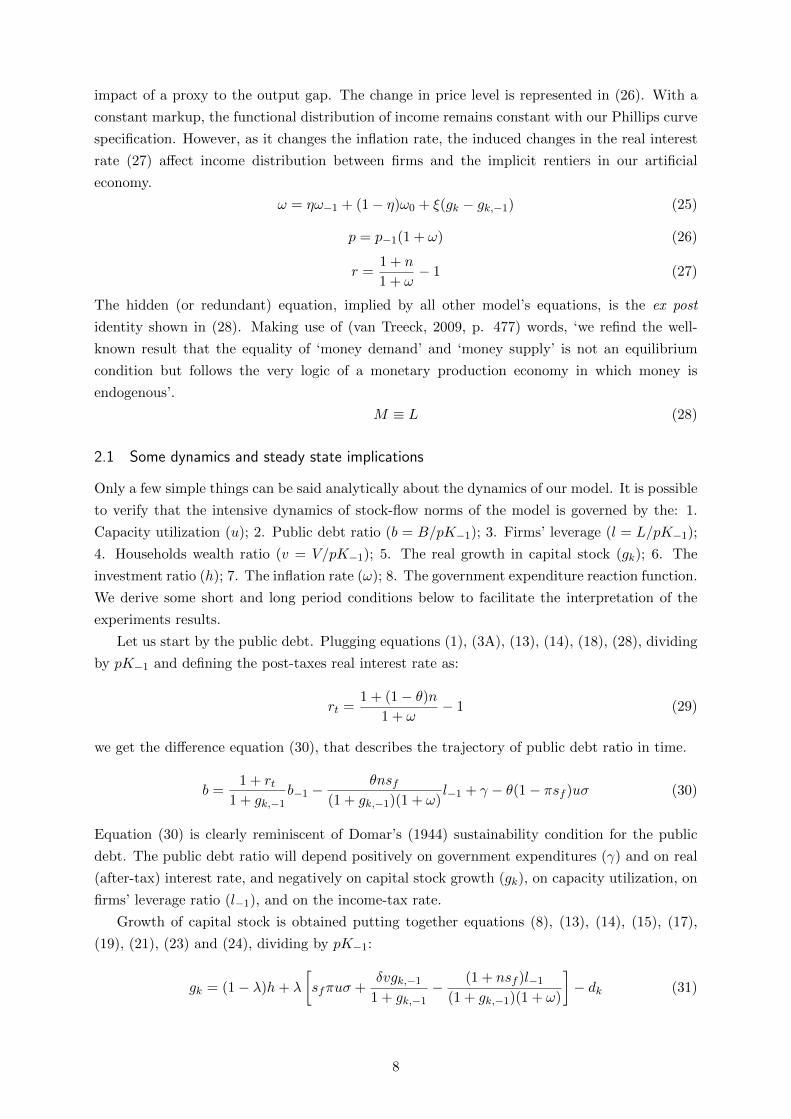
impact of a proxy to the output gap. The change in price level is represented in (26). With a

constant markup, the functional distribution of income remains constant with our Phillips curve

specification. However, as it changes the inflation rate, the induced changes in the real interest

rate (27) affect income distribution between firms and the implicit rentiers in our artificial

economy.

ω = ηω−1 + (1− η)ω0 + ξ(gk − gk,−1) (25)

p = p−1(1 + ω) (26)

r =1 + n

1 + ω− 1 (27)

The hidden (or redundant) equation, implied by all other model’s equations, is the ex post

identity shown in (28). Making use of (van Treeck, 2009, p. 477) words, ‘we refind the well-

known result that the equality of ‘money demand’ and ‘money supply’ is not an equilibrium

condition but follows the very logic of a monetary production economy in which money is

endogenous’.

M ≡ L (28)

2.1 Some dynamics and steady state implications

Only a few simple things can be said analytically about the dynamics of our model. It is possible

to verify that the intensive dynamics of stock-flow norms of the model is governed by the: 1.

Capacity utilization (u); 2. Public debt ratio (b = B/pK−1); 3. Firms’ leverage (l = L/pK−1);

4. Households wealth ratio (v = V/pK−1); 5. The real growth in capital stock (gk); 6. The

investment ratio (h); 7. The inflation rate (ω); 8. The government expenditure reaction function.

We derive some short and long period conditions below to facilitate the interpretation of the

experiments results.

Let us start by the public debt. Plugging equations (1), (3A), (13), (14), (18), (28), dividing

by pK−1 and defining the post-taxes real interest rate as:

rt =1 + (1− θ)n

1 + ω− 1 (29)

we get the difference equation (30), that describes the trajectory of public debt ratio in time.

b =1 + rt

1 + gk,−1b−1 −

θnsf(1 + gk,−1)(1 + ω)

l−1 + γ − θ(1− πsf )uσ (30)

Equation (30) is clearly reminiscent of Domar’s (1944) sustainability condition for the public

debt. The public debt ratio will depend positively on government expenditures (γ) and on real

(after-tax) interest rate, and negatively on capital stock growth (gk), on capacity utilization, on

firms’ leverage ratio (l−1), and on the income-tax rate.

Growth of capital stock is obtained putting together equations (8), (13), (14), (15), (17),

(19), (21), (23) and (24), dividing by pK−1:

gk = (1− λ)h+ λ

[sfπuσ +

δvgk,−11 + gk,−1

−(1 + nsf )l−1

(1 + gk,−1)(1 + ω)

]− dk (31)

8

Besides the obvious elements that influence growth in the short period, that is, the investment

ratio (h) and the depreciation of the capital stock (dk), it is remarkable the direct influence of

leverage, households’ wealth, retained earnings, the inflation rate (ω) and gk,−1. Such effects

emerge as a consequence of banks’ risk assessment.

The short period dynamics of capacity utilization is obtained using equations (3A), (4), (8),

(12), (13), (14), (17), (18), (21), (24).

u =φ

[(1− λ)h+ γ +

λδvgk,−11 + gk,−1

+nα(1− θ)(sf l−1 + b−1) + α3v−1 − λ(1 + nsf )l−1

(1 + gk,−1)(1 + ω)

](32)

with

φ =1

[1− λsfπ − α(1− θ)(1− πsf )]σ(33)

where φ can be interpreted as the Keynesian multiplier of the model, which is influenced by the

consumption out of income and distributed profits and the respective propensities to consume,

by the profit share and the retention rate. The effects of λ on capacity utilization resemble those

on gk, as by definition investment ratio appears in both variables. If we consider, to simplify,

that λ = 0, then:

u =1

[1− α(1− θ)(1− πsf )]σ

[h+ γ +

nα(1− θ)(sf l−1 + b−1) + α3v−1(1 + gk,−1)(1 + ω)

](32A)

In a single period, capacity utilization will be the result of the autonomous components of

demand times the multiplier effect. Namely, the autonomous components are the government

expenditure (γ), the investment (h), and the consumption out of interest income and out of

wealth, all as ratios of capital stock. Capacity utilization will also be influenced by lagged gk

and the inflation rate ω, levied on nominal financial stocks (wealth) and flows (interest income).

Households’ wealth ratio can be calculated by plugging equations (7), (8), (13), (14), (18)

and (19), again dividing by pK−1:

v =(1− α3 − δ)v−1

(1 + ω)(1 + gk,−1 − δ)+

(1− θ)(1− α)

1 + gk,−1 − δ

[(1 + gk,−1)(1− πsf )uσ +

n(sf l−1 + b−1)

1 + ω

](34)

Given the (constant) parameters, v depends on capacity utilization, on the inflation rate and on

the lagged growth in capital stock.

Finally, we get firms’ outstanding loans (or leverage) ratio (l = L/pK−1), whose determinants

are quite similar for those of v, by using equations (8), (13), (14), (15), (17), (19), (20) and (24):

l = (1− λ)

[h− sfπuσ −

δvgk,−11 + gk,−1

+(1 + nsf )l−1

(1 + gk,−1)(1 + ω)

](35)

In the automatic stabilizer regime, the system is completed by equations (16) and (25). In

the countercyclical and austerity fiscal regimes, besides (16) and (25), an eighth equation is

attached to the system, namely (3B) or (3C), respectively.

From equations (30), (34), (35), (31) we get the steady state solutions, assuming that λ = 0

in the long-run:

b∗ =(1 + g∗k)[γ − θ(1− πsf )u∗σ]

g∗k − r∗t−

nθsf l∗

(g∗k − r∗t )(1 + ω∗)(36)

9

v∗ =(1− θ)(1− α)(1 + ω∗)

g∗k(1 + ω∗) + ω∗(1− δ) + α3

[(1 + g∗k)(1− πsf )u∗σ +

n(sf l∗ + b∗)

1 + ω∗

](37)

l∗ =(1 + g∗k)(1 + ω∗)

g∗k(1 + ω∗) + ω∗ − nsf

[h∗ − sfπu∗σ −

δv∗g∗k1 + g∗k

](38)

g∗k = h∗ − dk (39)

As we assume in the simulations that inflation converges to a long-run fixed point (with η <

1), and u converges to the neighborhood of un through the firms’ adaptation of the investment

ratio h, gk will have a crucial role in determining the steady state conditions. For instance,

as clear in (39), g∗k depends precisely on the trajectory of h. Therefore, the evolution of h in

time, which is influenced by the short-run aggregate demand conditions – on its turn influenced

by private sectors’ financial decisions –, is of ultimate importance for the determination of the

steady state norms.

Needless to say, the system of difference equations that emerges from our model is too com-

plex for obtaining an analytical solution. For this reason, following most of the SFC practitioners

(Caverzasi and Godin, 2015), we do some simulated numerical experiments with calibrated pa-

rameter values in order to analyze our model’s implications.

3 Experiments

In this section, we discuss some experiments that show how private financial behavior influences

the fiscal variables (public deficit and debt), under different fiscal regimes. By financial behavior,

we mean households’, banks’ and firms’ decisions that affect theirs balance sheets and investment

financing. Given the desired investment (Id,15), three parameters are crucial in determining the

financing constraints that yields the effective investment (I,21): 1. the retention rate sf , which

determines firms’ own funding; 2. the lender’s (banks) risk perception λ, which influences

supplied bank lending; 3. the share of wealth households allocate as stocks δ, which affects the

funding from the stock market.

We perform four experiments changing three parameters:

1. A credit crunch caused by a transitory increase in lender’s risk (λ), combined with a fiscal

regime where only automatic stabilizers operate (3A). In order to evaluate the importance

of the inflation behavior for the outcomes, we analyze some combinations of parameters η

and ξ in the Phillips curve (25);

2. A same-sized credit crunch, with the other two fiscal regimes: the countercyclical (3B)

and the austere (or pro-cyclical, 3C);

3. A permanent decrease in the share of households portfolio allocated in stock (δ), leading

to a change in firms’ financing composition, considering the three fiscal regimes;

4. A permanent decrease in firms’ desired leverage ratio – which we introduce in the corre-

sponding subsection (3.4) –, that trigger changes in the retention rate (sf ), with all the

above-mentioned fiscal regimes;

The first two experiments are associated with credit (and business) cycles, while the latter

two may be related to the so-called financialization (see Epstein, 2005; Lavoie, 2008; van Treeck,

10

2009, among others). The effects of a reduction in households demand for stocks are similar

to those of a reduction in initial public offering (IPO) as a means of financing investment. In

the case of an increase in the retention rate sf , resulting from the firms’ desire to reduce their

leverage, our experiment means a reversal of the downsize and distribute (dividends) paradigm

(Aglietta, 2000; Lazonick and O’Sullivan, 2000, inter alia).

All the trajectories are compared with the same baseline steady state. The results are

evaluated according to two criteria: the time for economic activity to recover and the public

debt ratio (b) trajectory. We also focus on the role of inflation, of autonomous consumption,

fiscal policy and their interaction in the traverse to the steady state.

Of course this is a theoretical exercise. It shows where the economy tends to assuming

a constant state of expectations.6 In practice, the state of expectations – as well as other

parameters we consider given – do not remain constant long enough for that to happen (Keynes,

1936). Because of that, the short and medium-run effects (or the traverse) of policies seem to be

the relevant time horizon from the policy maker standpoint. Besides, one should not disregard

that short and medium run events may influence long run conditions, or while analyzing the

transition, that ‘trajectories in which the balance sheets of large parts or even whole institutional

sectors (as productive companies or households) become more fragile can lead to regime changing

structural breaks due to endogenous reasons’ (Macedo e Silva and Dos Santos, 2011, p. 113).

This means that, even though the model converges to a steady state, one should not ignore that

very discrepant trajectories can lead to a structural disruption.

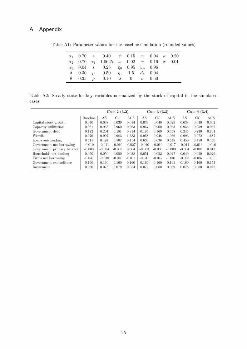
Calibrated parameter values in the baseline and the steady state for selected variables in

each scenario, for each fiscal regime presented, can be found in the appendix.

3.1 Effects of a transitory shock in lender’s risk (λ): non-reactive fiscal expenditure

In this experiment, we create a temporary upward shock to lender’s risk,7 triggering a credit

crunch. Results are presented for different combinations of parameters η and ξ in equation

(25): 1. if η = 0, ξ = 0, the inflation rate is constant over time; 2. if η = 0.75, ξ = 0.75,

current inflation is sensitive to past inflation and to the proxy of the output gap (∆gk); 3.

η = 0.95, ξ = 1.5 means that current inflation is more inertial and is more sensitive to the

output gap proxy. The changes in the inflation parameters make it easier to emphasize the role

of inflation in the outcomes. The shock in λ means, from equation (24), the part of firms’ desired

investment to be financed by banks will fall. Furthermore, it requires firms to repay a share λ

of past stock of loans since loans are all short-term, thus outstanding credit will actually fall.

Government expenditures follow the automatic stabilizer (AS) regime, as defined in equation

(3A).

Chart 1a shows the dynamics of public debt ratio after the credit crunch for different inflation

parameters. The meaningful increase in this ratio is a result of several phenomena, as one can

infer by checking (30).

First, the contraction in credit determines a considerable reduction in effective investment

ratio (gk, see 31), which by its own exerts a negative impact on the dynamics of b. Through

6Except for the investment ratio h.7We introduce in the model a simple exponential function for the lender risk shock to be transitory, given byλ = λa

−1 +λ0. For λ to be time-decreasing and converge to 0, a > 1. The shock takes place in period t = 5, withan increase of 4 percentage points in λ0, and a is set to be 1.03. If t > 5 then λ0 = 0.

11

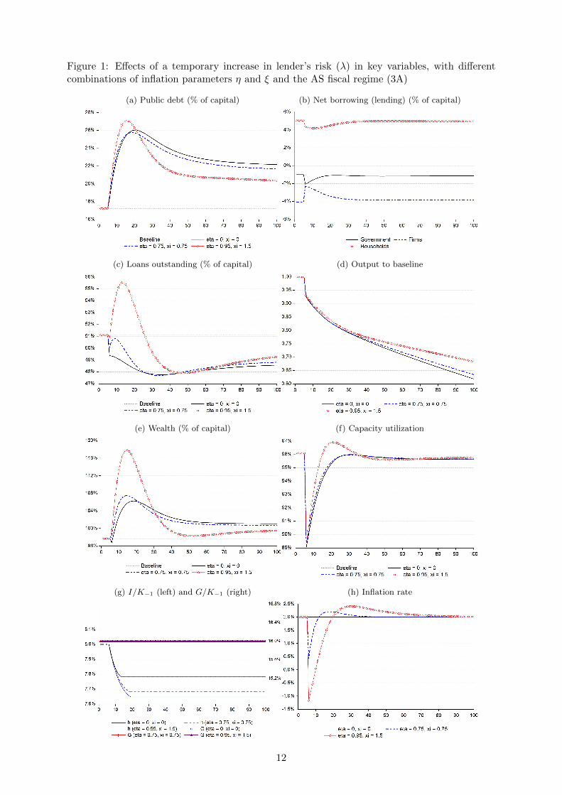
Figure 1: Effects of a temporary increase in lender’s risk (λ) in key variables, with differentcombinations of inflation parameters η and ξ and the AS fiscal regime (3A)

(a) Public debt (% of capital) (b) Net borrowing (lending) (% of capital)

(c) Loans outstanding (% of capital) (d) Output to baseline

(e) Wealth (% of capital) (f) Capacity utilization

(g) I/K−1 (left) and G/K−1 (right) (h) Inflation rate

12

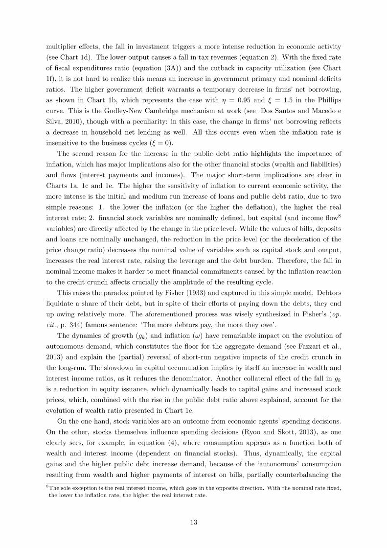
multiplier effects, the fall in investment triggers a more intense reduction in economic activity

(see Chart 1d). The lower output causes a fall in tax revenues (equation 2). With the fixed rate

of fiscal expenditures ratio (equation (3A)) and the cutback in capacity utilization (see Chart

1f), it is not hard to realize this means an increase in government primary and nominal deficits

ratios. The higher government deficit warrants a temporary decrease in firms’ net borrowing,

as shown in Chart 1b, which represents the case with η = 0.95 and ξ = 1.5 in the Phillips

curve. This is the Godley-New Cambridge mechanism at work (see Dos Santos and Macedo e

Silva, 2010), though with a peculiarity: in this case, the change in firms’ net borrowing reflects

a decrease in household net lending as well. All this occurs even when the inflation rate is

insensitive to the business cycles (ξ = 0).

The second reason for the increase in the public debt ratio highlights the importance of

inflation, which has major implications also for the other financial stocks (wealth and liabilities)

and flows (interest payments and incomes). The major short-term implications are clear in

Charts 1a, 1c and 1e. The higher the sensitivity of inflation to current economic activity, the

more intense is the initial and medium run increase of loans and public debt ratio, due to two

simple reasons: 1. the lower the inflation (or the higher the deflation), the higher the real

interest rate; 2. financial stock variables are nominally defined, but capital (and income flow8

variables) are directly affected by the change in the price level. While the values of bills, deposits

and loans are nominally unchanged, the reduction in the price level (or the deceleration of the

price change ratio) decreases the nominal value of variables such as capital stock and output,

increases the real interest rate, raising the leverage and the debt burden. Therefore, the fall in

nominal income makes it harder to meet financial commitments caused by the inflation reaction

to the credit crunch affects crucially the amplitude of the resulting cycle.

This raises the paradox pointed by Fisher (1933) and captured in this simple model. Debtors

liquidate a share of their debt, but in spite of their efforts of paying down the debts, they end

up owing relatively more. The aforementioned process was wisely synthesized in Fisher’s (op.

cit., p. 344) famous sentence: ‘The more debtors pay, the more they owe’.

The dynamics of growth (gk) and inflation (ω) have remarkable impact on the evolution of

autonomous demand, which constitutes the floor for the aggregate demand (see Fazzari et al.,

2013) and explain the (partial) reversal of short-run negative impacts of the credit crunch in

the long-run. The slowdown in capital accumulation implies by itself an increase in wealth and

interest income ratios, as it reduces the denominator. Another collateral effect of the fall in gk

is a reduction in equity issuance, which dynamically leads to capital gains and increased stock

prices, which, combined with the rise in the public debt ratio above explained, account for the

evolution of wealth ratio presented in Chart 1e.

On the one hand, stock variables are an outcome from economic agents’ spending decisions.

On the other, stocks themselves influence spending decisions (Ryoo and Skott, 2013), as one

clearly sees, for example, in equation (4), where consumption appears as a function both of

wealth and interest income (dependent on financial stocks). Thus, dynamically, the capital

gains and the higher public debt increase demand, because of the ‘autonomous’ consumption

resulting from wealth and higher payments of interest on bills, partially counterbalancing the

8The sole exception is the real interest income, which goes in the opposite direction. With the nominal rate fixed,the lower the inflation rate, the higher the real interest rate.

13

fall in actual investment. The increase in public debt ratio is a result of the increased public

deficit and, at the same time, cushions the transition to the steady state, as it raises households

consumption and thereby firm’s savings.

The sensitivity of inflation to its determinants strongly affects the trajectory of assets (or

liabilities) ratios. The more intense is the deflationary impact of the shock, the higher is the

initial peak in asset (liability) ratios. Low inflation (or high deflation) implies higher values for

financial stocks and flows. In our (simple) model, this provides a higher floor to aggregate de-

mand; in consequence, u will converge more readily to the to the neighborhood of un, dampening

the downward adjustments by entrepreneurs investment decisions (which for instance cause a

fall in the investment ratio h). This result, of course, does not mean that price flexibility is a

boon. In a more realistic (and far more complicated) model, a quick increase in firms’ loans and

real interest payments ratio might well lead to bankruptcy and to further increases in lender’s

risk.

Last but not least, as u converges to un, what changes other steady state conditions (such as

the wealth ratio and the very growth rate) is the adaptive investment function (see Chart 1g and

16), through its effects in gk – see equations (36), (37), (38) and (39). As long as entrepreneurs

react to short-run events and do achieve some target, in the present case the neighborhood of the

desired capacity utilization, there are no endogenous reasons for them to change their behavior.

Thus our model presents path dependency, as even a transitory shock leads to permanent effects

on growth and stock-flow norms.

3.2 Effects of a transitory shock in lender’s risk (λ): reactive fiscal expenditure

The central motivation for the experiment of the current section is to assess how the choice of

fiscal regime – countercyclical (3B) or austere (3C) – affects the trajectories of fiscal variables.

Lender’s risk shock is equivalent. We consider the fixed inflation (η = 0, ξ = 0) and the sensitive

inflation rate (η = 0.95, ξ = 1.5) cases.

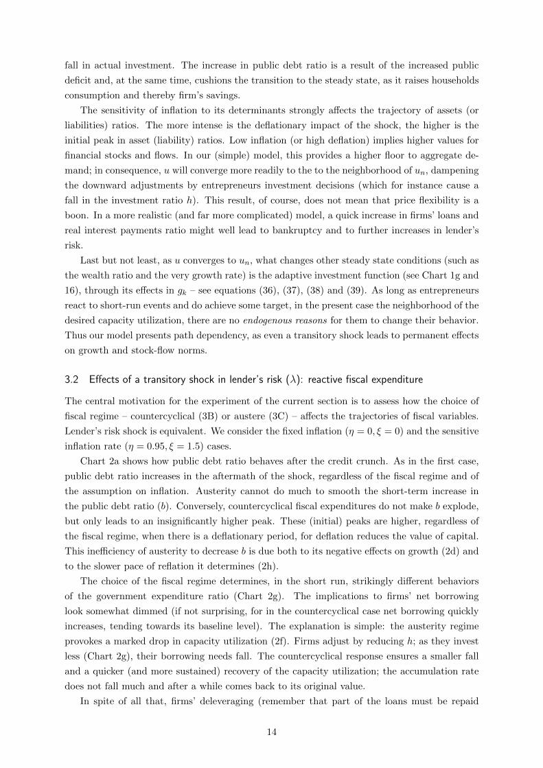
Chart 2a shows how public debt ratio behaves after the credit crunch. As in the first case,

public debt ratio increases in the aftermath of the shock, regardless of the fiscal regime and of

the assumption on inflation. Austerity cannot do much to smooth the short-term increase in

the public debt ratio (b). Conversely, countercyclical fiscal expenditures do not make b explode,

but only leads to an insignificantly higher peak. These (initial) peaks are higher, regardless of

the fiscal regime, when there is a deflationary period, for deflation reduces the value of capital.

This inefficiency of austerity to decrease b is due both to its negative effects on growth (2d) and

to the slower pace of reflation it determines (2h).

The choice of the fiscal regime determines, in the short run, strikingly different behaviors

of the government expenditure ratio (Chart 2g). The implications to firms’ net borrowing

look somewhat dimmed (if not surprising, for in the countercyclical case net borrowing quickly

increases, tending towards its baseline level). The explanation is simple: the austerity regime

provokes a marked drop in capacity utilization (2f). Firms adjust by reducing h; as they invest

less (Chart 2g), their borrowing needs fall. The countercyclical response ensures a smaller fall

and a quicker (and more sustained) recovery of the capacity utilization; the accumulation rate

does not fall much and after a while comes back to its original value.

In spite of all that, firms’ deleveraging (remember that part of the loans must be repaid

14

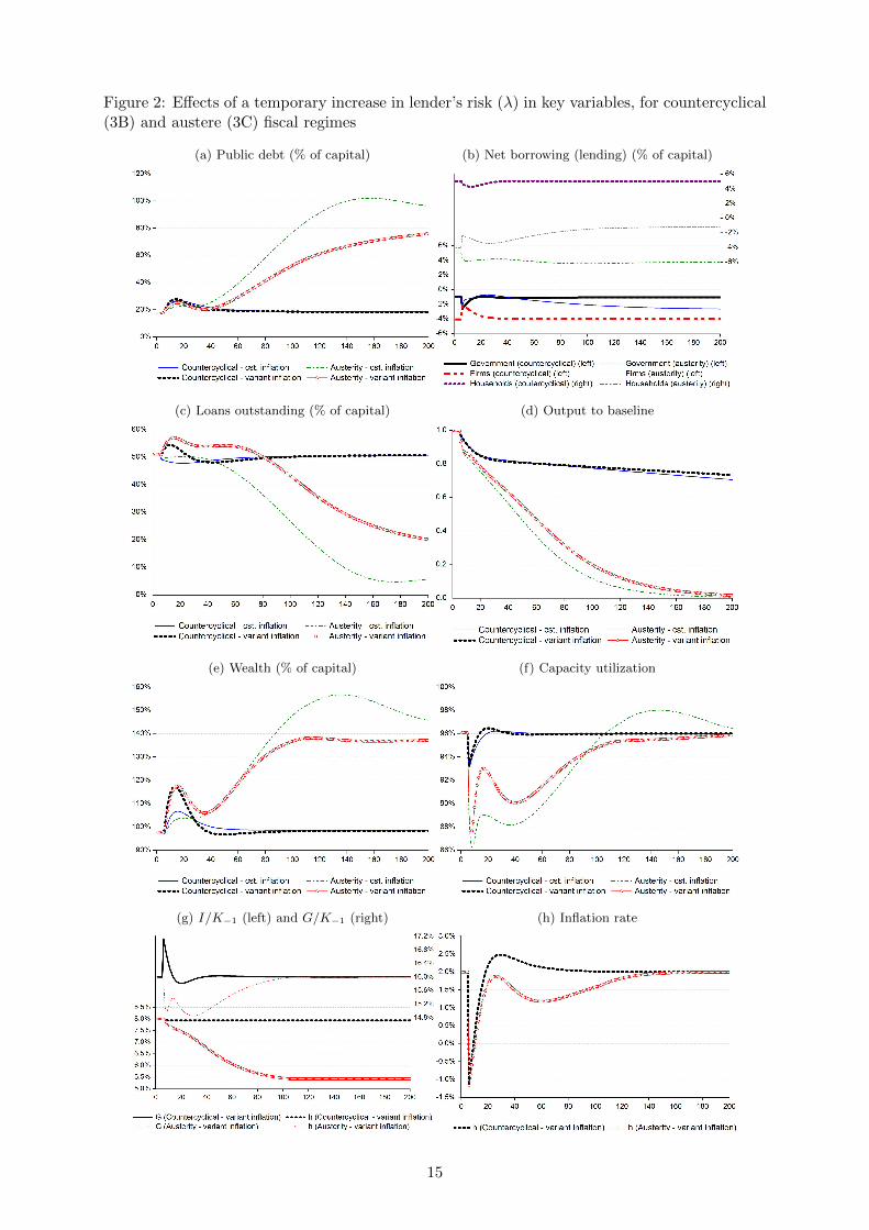
Figure 2: Effects of a temporary increase in lender’s risk (λ) in key variables, for countercyclical(3B) and austere (3C) fiscal regimes

(a) Public debt (% of capital) (b) Net borrowing (lending) (% of capital)

(c) Loans outstanding (% of capital) (d) Output to baseline

(e) Wealth (% of capital) (f) Capacity utilization

(g) I/K−1 (left) and G/K−1 (right) (h) Inflation rate

15

when λ > 0) is much more painful in the austerity case, given the effect of the slower deflation

on the loans ratio (Chart 2c). Firms have also to cope, in this context, with a higher burden of

debt; nominal profits fall not only because demand is falling (reducing real profits as well) but

because of the more prolonged deflation. However, even when austerity does not cause deflation,

we observe a longer time for de-leveraging to happen.

In the austerity scenario, it takes a long time for the desired investment rate (h) and the

effective (gk) accumulation rate to reach their new and much lower level (Chart 2g). This implies,

of course, a much lower long-run rate of growth. As the inflation rate converges to 2% (Chart

2h)9 and u to un (Chart 2f), b∗ (36) and v∗ (37) converge to higher levels, because of the lower

g∗k.

This means that the attempt to reduce government expenditures triggered by the increase

in the public debt – that would completely sound if based on a purely (and partial) analysis of

the public debt ‘law of motion’ (30) – does not deliver what it promises because of the feedback

effects on capacity utilization (Chart 2f) and on the accumulation rate (Chart 2g). In our

model’s longer period, the attempts to reduce the public debt ratio through austerity backfire,

creating conditions for lower long-run growth and higher public debt ratio.

The dynamics of the public debt ratio in the countercyclical policy is similar to the austerity

case in the short-run and very different in the long period. In the short run, the higher growth

rate compensates for the bigger increase in public expenditure and deficit. In the long-run, the

faster convergence of u towards un entails higher steady state accumulation rate (gk). As a

consequence, b∗ (36) in the countercyclical case will converge to a value only slightly higher than

the baseline.

3.3 Effects of a permanent decrease in households demand for shares (δ)

A permanent fall in the demand for shares depresses equities price (8), causing capital losses

and an abrupt fall in households wealth. It increases the leverage of firms (Chart 3c), as the

finance raised by firms through the issuance of shares drops. The channel through which it

affects aggregate demand is the fall in consumption out of wealth – a component of autonomous

demand –, which dynamically reduces investment. The higher the propensity to consume out of

wealth, the higher will be the impact of the shock. As in our model, with its parametrization,

the consumption out of wealth represent about 16% of total consumption, the effect on capacity

utilization is not very large – as Chart 3f shows.

The logic of the shock propagation and its implications can be described as follows: in the

absence of an increase in government expenditure to compensate for the fall in private demand,

growth diminishes through changes in the investment ratio; as before, the lower growth results

in higher wealth and interest income ratios. Government debt ratio will once more increase

in the aftermath of the shock, but in this case this change is very marginally influenced by

the dynamics of inflation. The main short-run factor is the fall in capacity utilization; in the

long-run, it becomes the fall in capital stock growth.

9At this point, it is necessary to clarify that the conventional Phillips curve may affect the results. If we included,instead, the conflicting claims or a Phillips curve with a flat segment as suggested by Godley and Lavoie (2007b),then it would be no longer obvious that reflation would occur in the austerity case. From Okun’s law we knowthat employment and growth are strictly related in a way that lower growth results in higher unemployment,which reduces the bargaining power of workers.

16

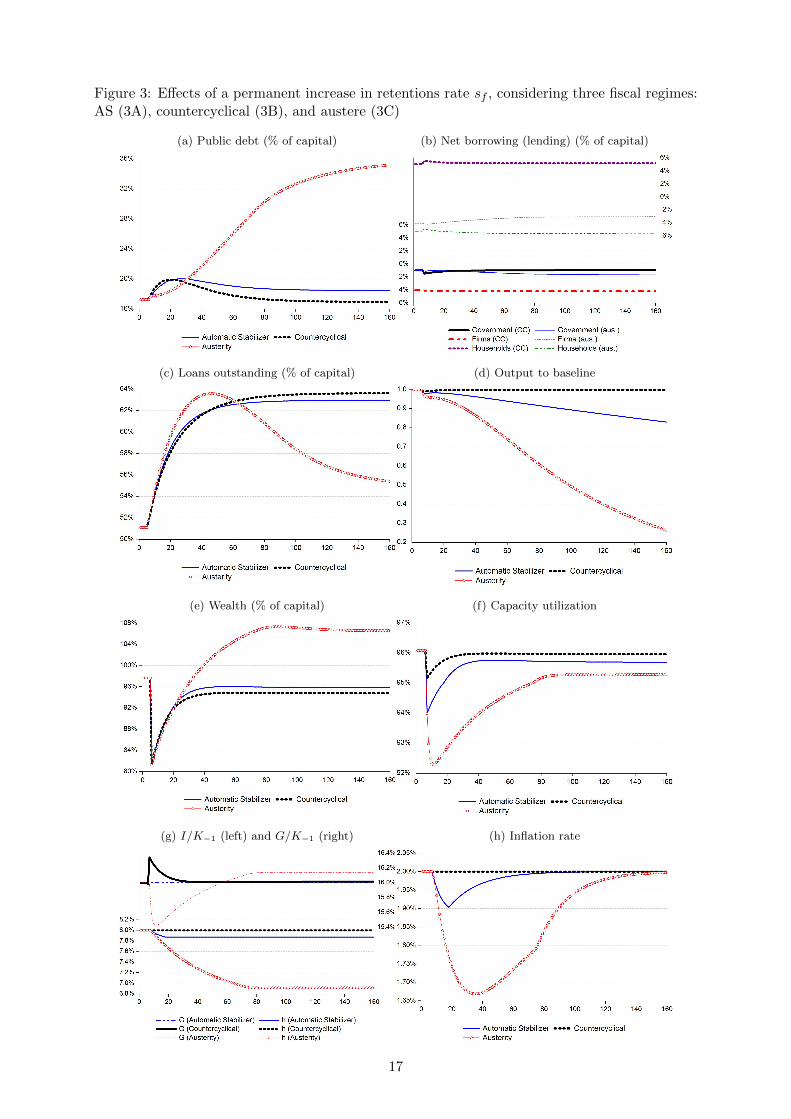
Figure 3: Effects of a permanent increase in retentions rate sf , considering three fiscal regimes:AS (3A), countercyclical (3B), and austere (3C)

(a) Public debt (% of capital) (b) Net borrowing (lending) (% of capital)

(c) Loans outstanding (% of capital) (d) Output to baseline

(e) Wealth (% of capital) (f) Capacity utilization

(g) I/K−1 (left) and G/K−1 (right) (h) Inflation rate

17

It is worth highlighting that the growth effects in this case are not as pronounced as in

previous experiments. In the countercyclical case, there is no loss in output growth at all (see

Chart 3d); the reaction of government allows for the increase in households’ savings. Even in

the austerity case, the economy grows about 3% in the steady state, as compared to the 4%

baseline’s growth rate, while households’ savings fall below the initial level as a result of the

increased consumption out of wealth (Chart 3e). Remarkably, government expenditure ratio to

capital goes above the initial level in the austerity case in the longer period (Chart 3g), yet the

growth rate of the economy is not fully restored.

3.4 Effects of a permanent decrease in the target leverage ratio

In this experiment we add an equation to our benchmark model, creating a mechanism for firms

to pursue their (exogenous) target leverage ratio (lT ) through changes in the retention rate (sf ),

as described in the equation below:

sf = sf,−1 + κ(l−1 − lT ) (40)

Equation (40) means that firms will retain more profits in order to reduce their leverage.

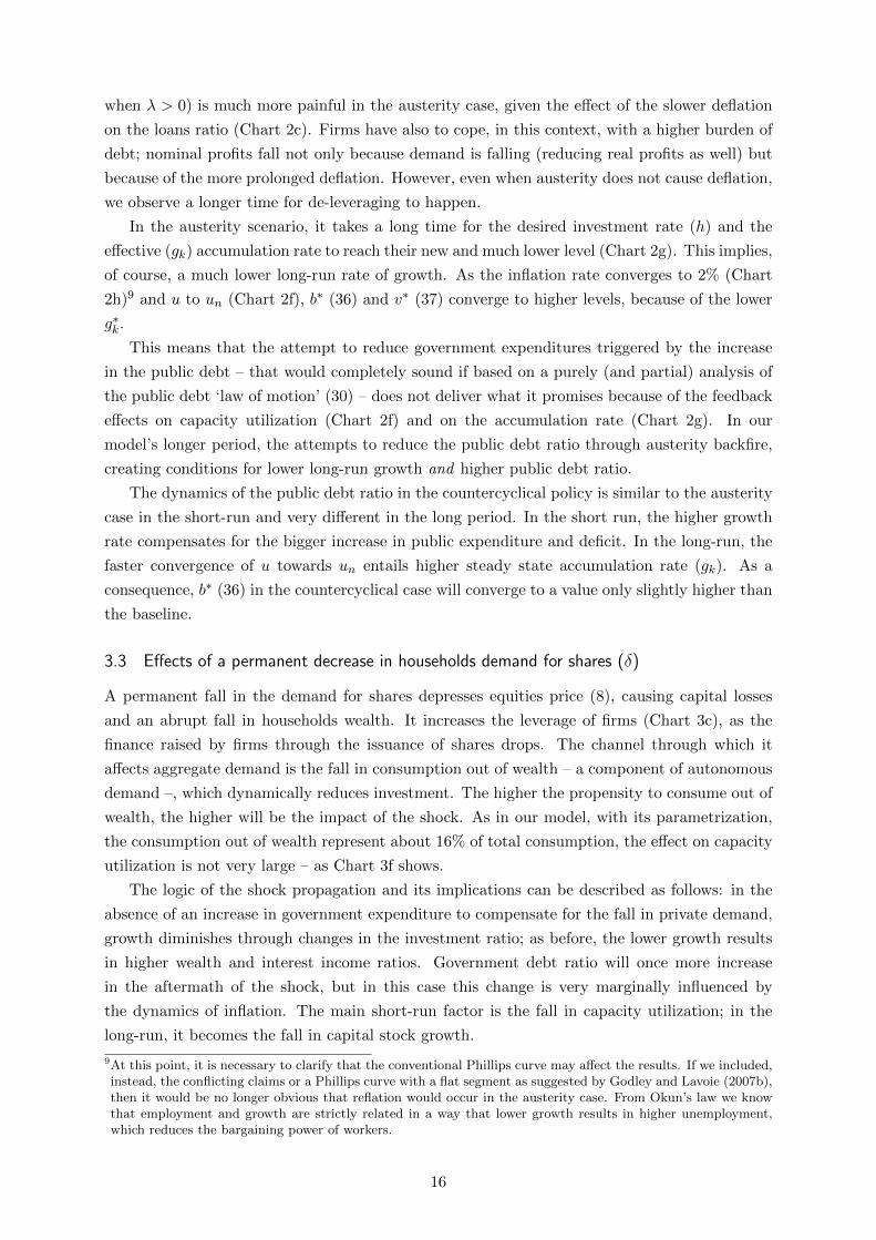
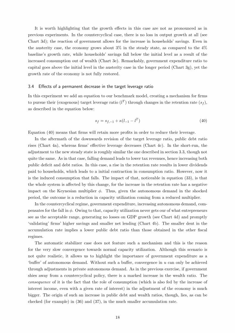
In the aftermath of the downwards revision of the target leverage ratio, public debt ratio

rises (Chart 4a), whereas firms’ effective leverage decreases (Chart 4c). In the short-run, the

adjustment to the new steady state is roughly similar the one described in section 3.3, though not

quite the same. As in that case, falling demand leads to lower tax revenues, hence increasing both

public deficit and debt ratios. In this case, a rise in the retention rate results in lower dividends

paid to households, which leads to a initial contraction in consumption ratio. However, now it

is the induced consumption that falls. The impact of that, noticeable in equation (33), is that

the whole system is affected by this change, for the increase in the retention rate has a negative

impact on the Keynesian multiplier φ. Thus, given the autonomous demand in the shocked

period, the outcome is a reduction in capacity utilization coming from a reduced multiplier.

In the countercyclical regime, government expenditure, increasing autonomous demand, com-

pensates for the fall in φ. Owing to that, capacity utilization never gets our of what entrepreneurs

see as the acceptable range, generating no losses on GDP growth (see Chart 4d) and promptly

‘validating’ firms’ higher savings and smaller net lending (Chart 4b). The smaller dent in the

accumulation rate implies a lower public debt ratio than those obtained in the other fiscal

regimes.

The automatic stabilizer case does not feature such a mechanism and this is the reason

for the very slow convergence towards normal capacity utilization. Although this scenario is

not quite realistic, it allows us to highlight the importance of government expenditure as a

‘buffer’ of autonomous demand. Without such a buffer, convergence in u can only be achieved

through adjustments in private autonomous demand. As in the previous exercise, if government

shies away from a countercyclical policy, there is a marked increase in the wealth ratio. The

consequence of it is the fact that the role of consumption (which is also fed by the increase of

interest income, even with a given rate of interest) in the adjustment of the economy is much

bigger. The origin of such an increase in public debt and wealth ratios, though, lies, as can be

checked (for example) in (36) and (37), in the much smaller accumulation rate.

18

Figure 4: Effects of a permanent increase in retentions rate sf , considering three fiscal regimes:automatic stabilizer (3A), countercyclical (3B), and austere (3C)

(a) Public debt (% of capital) (b) Net borrowing (lending) (% of capital)

(c) Loans outstanding (% of capital) (d) Output to baseline

(e) Wealth (% of capital) (f) Capacity utilization

(g) I/K−1 (left) and G/K−1 (right) (h) Inflation rate

19

The paucity of ‘new’ (government) autonomous demand in the automatic stabilizer fiscal

regime is a sufficient condition for the relatively (to the countercyclical regime) increased public

debt and lower growth.

Under austerity, the government does manage to revert the initial impact on the primary

deficit, which even increases, dampening the growing trend of the public debt ratio. However,

the continued contraction in its expenditures (so as to reduce the primary deficit) reduces growth

even more than in the AS regime. Again, private consumption will initially lead the way to the

new steady state, but at the cost of a huge fall in households’ net borrowing ratio.

Interestingly, despite the lower steady state primary deficit (see Appendix A2), the nominal

deficit ratio is much bigger (see Chart 4b). Government still provide in the (very) long-run

the conditions for the private demand (via higher interest payments and higher public debt) to

stabilize the system, but the transitional accommodation is qualitatively worse, for it is partially

obtained by means of higher interest payments on public debt.

4 Final remarks

As Keynes and Minsky taught us, monetary economies must be studied as a web of intercon-

nected agents: in macroeconomics one cannot ignore that a group’s (or institutional sector’s)

decisions may affect decisively the balance sheet of the others, triggering a reaction that may be

inconsistent with the initial desired change. The central role of the interactions between public

and private sectors was highlighted by both Minsky and Godley. Our model has explored some

of these interactions.

First, the model suggests that public debt and deficit ratios are strongly connected to the

private financial behavior. It confirms and explores Keynesian intuitions according to which it

is misleading to depict the behavior of public deficit and debt ratios as the direct result of the

fiscal stance. All experiments creating contractionary shocks in parameters influencing firms’

financing of investment – namely, an increase in lender’s risk, an increase in firms’ retention

rate and a fall in household demand for stocks – lead to permanently higher public debt and

nominal deficit ratios. This relation is causal by a logical reason: contractionary private financial

behavior precedes temporally fiscal deterioration.

Broadly speaking, the channel of transmission is the fall in economic activity and capital

accumulation that results from the contraction provoked by the shift in private financing deci-

sions, which lowers considerably government tax revenues, generating bigger deficit and debt.

Moreover, the effects of such a fall on the inflation rate were shown to be crucial to the trajectory

of the public debt ratio. The higher the inflation rate sensitiveness to current economic activity,

the greater the deflationary trend and, as a consequence, the bigger the increase in public debt

ratio. This is the Fisherian effect.

We deliberately studied only contractionary cases (which may trigger government austere

behavior), or the downswing phase of the business cycle. Nonetheless, the model also implies

that more permissive (or debt-tolerant) private financing conditions lead to a fiscal improvement,

in the sense that public deficit and debt to GDP ratios required to equilibrate private agents’

portfolios will be lower.

Second, our simulations point out that some fiscal deterioration in the aftermath of con-

20

tractionary private financial behavior takes place whatever the fiscal regime. In the austerity

case we studied, government expenditure falls to counterbalance the trend of higher primary

deficit ratio after the shock. The government withdraws autonomous demand precisely when it

is more necessary. This behavior pushes most of the adjustment to the new financial condition

to the private sector, sparking a negative spiral that leads to a fall in long-run output growth.

The change in GDP growth is a result of the temporarily lower government expenditure, which

induces the downward adjustment of the investment ratio. As a consequence, in the absence of

further exogenous changes in the system, capital stock growth is permanently reduced in austere

fiscal regime, suggesting the existence of path dependence in our artificial economy.

Conversely, the reason why countercyclical fiscal policy works is objective. In a regime where

in the very beginning of the shock government expenditures increase, aggregate demand, firms’

profits and capacity utilization recovery run in a faster pace, halting the fall in investment

ratio. On the fiscal side, outcomes are not substantially worse than those produced by austerity

in the short-run. In the longer term, the countercyclical fiscal regime delivers better results

than austerity, because of the mutual interactions between fiscal policy, economic activity and

inflation. Whilst countercyclical fiscal policy contributes to counterbalance the deflationary

trend and the fall in demand, which is favorable for the recovery, in most cases austerity adds

fuel to both.

We have shown that this is the more likely reason why austerity is not capable of deliver-

ing better fiscal results than countercyclical policy. In a contractionary financial environment,

indebted private agents badly need an increase in cash flows, to honor their financial commit-

ments. In a closed economy, these cash flows can only be provided by the public deficit. In

addition, stabilization is influenced by public debt itself, which is not only a result of people’s

spending decisions and fiscal policy, for public debt also influences the spending decisions; the

mutual interactions between public debt and effective demand will jointly determine a particular

trajectory for the public debt (Ryoo and Skott, 2013).

In their full employment SFC model, Ryoo and Skott (2013, p. 524) conclude that ‘fiscal

deficits and a rise in public debt are necessary if the government wants to maintain full em-

ployment following a decline in demand’, and that ‘fluctuations in private sector confidence and

financial behavior can and should be offset by variations in public debt’ (op. cit., p.525). We

agree in spirit with them, but we go beyond: in closed economies, meaningful changes in pri-

vate state of expectations or objective shifts in private financial behavior do not give the ‘Big

Government’ a real option, in terms of avoiding a deterioration in fiscal variables, even if not

pursuing full employment.

Further extensions of this model should include the external sector. Similar processes in open

economies may lead to different adjustment dynamics, depending on their size, openness, on the

scale and pervasiveness of the crisis, on the currency-sovereignty, on the position of the currency

in the international monetary hierarchy, on the adoption of cooperative or beggar-thy-neighbor

international policies, among other features.

21

References

Aglietta, M. (2000). Shareholder value and corporate governance: some tricky questions. Econ-omy and Society, 29(1):146–159.

Allain, O. (2015). Tackling the instability of growth: a Kaleckian-Harrodian model with anautonomous expenditure component. Cambridge Journal of Economics, 39(5):1351–1371.

Asensio, A., Lang, D., and Charles, S. (2012). Post Keynesian modeling: where are we, andwhere are we going to? Journal of Post Keynesian Economics, 34(3):393–412.

Bhaduri, A. and Marglin, S. (1990). Unemployment and the real wage: the economic basis forcontesting political ideologies. Cambridge Journal of Economics, 14(4):375–393.

Botta, A. (2013). Fiscal policy, Eurobonds, and economic recovery: heterodox policy recipesagainst financial instability and sovereign debt crisis. Journal of Post Keynesian Economics,35(3):417–441.

Caverzasi, E. and Godin, A. (2015). Post-Keynesian stock-flow-consistent modelling: a survey.Cambridge Journal of Economics, 39(1):157–187.

Chick, V. and Caserta, M. (1997). Provisional equilibrium and macroeconomic theory. In Arestis,P., Palma, G., and Sawyer, M., editors, Markets, Employment and Economic Policies: Essaysin Honour of G.C. Harcourt, volume Two, pages 223–37. Routledge, London.

Committeri, M. (1986). Some Comments on Recent Contributions on Capital Accumulation,Income Distribution and Capacity Utilization. Political Economy: Studies in the SurplusApproach, 2(2):161–186.

Davidson, P. (1978). Money and the real world. John Wiley & Sons, Nova York, 2a edicaoedition.

Domar, E. D. (1944). The “Burden of the Debt” and the National Income. The AmericanEconomic Review, 34(4):798–827.

Dos Santos, C. H. and Macedo e Silva, A. C. (2010). Revisiting ”New Cambridge”: The ThreeFinancial Balances in a General Stock–flow Consistent Applied Modeling Strategy. In LevyEconomics Institute of Bard College Working Paper Series, n. 594.

Dos Santos, C. H. and Zezza, G. (2008). A simplified, ’benchmark’, stock-flow consistent post-Keynesian growth model. Metroeconomica, 59(3):441–478.

Dumenil, G. and Levy, D. (1999). Being Keynesian in the Short Term and Classical in the LongTerm: The Traverse to Classical Long-Term Equilibrium. The Manchester School, 67(6):684–716.

Dutt, A. K. (1990). Growth, Distribution and Uneven Development. Cambridge UniversityPress, Cambridge, UK.

Epstein, G. A. (2005). Financialization and the world economy. Edward Elgar, Cheltenham,UK ; Northampton, MA.

Fazzari, S. M., Ferri, P. E., Greenberg, E. G., and Variato, A. M. (2013). Aggregate demand,instability, and growth. Review of Keynesian Economics, 1(1):1–21.

Fisher, I. (1933). The Debt-Deflation Theory of Great Depressions. Econometrica, 1(4):337–357.

Freitas, F. and Serrano, F. (2015). Growth Rate and Level Effects, the Stability of the Adjust-ment of Capacity to Demand and the Sraffian Supermultiplier. Review of Political Economy,27(3):258–281.

Godley, W. and Lavoie, M. (2007a). Fiscal policy in a stock-flow consistent (SFC) model. Journalof Post Keynesian Economics, 30(1):79–100.

Godley, W. and Lavoie, M. (2007b). Monetary economics: an integrated approach to credit,money, income, production and wealth. Palgrave Macmillan, New York, 1st edition.

Hein, E. (2012). The Macroeconomics of Finance-dominated Capitalism and its Crisis. Edward

22

Elgar, Cheltenham, UK and Northampton, MA, USA.

Hewitson, G. (1997). The post-Keynesian ’demand for credit’ model. Australian EconomicPapers, 36(68):127–143.

Hicks, J. (1974). The crisis in Keynesian economics. Basil Blackwell, Oxford.

Keynes, J. M. (1936). The General Theory of Employment, Interest and Money. Macmillan,London.

Lang, D. and Peretti, C. (2009). A strong hysteretic model of Okun’s Law: theory and apreliminary investigation. International Review of Applied Economics, 23(4):445–462.

Lavoie, M. (2006). A post-Keynesian amendment to the new consensus on monetary policy.Metroeconomica, 57(2):165–192.

Lavoie, M. (2008). Financialisation Issues in a Post-Keynesian Stock-Flow Consistent Model.Intervention, 5(2):331–356.

Lavoie, M. (2014). Post-Keynesian Macroeconomics: New Foundations. Edward Elgar, Chel-tenham (UK), Northampton (US).

Lavoie, M. (2016). Convergence Towards the Normal Rate of Capacity Utilization in Neo-Kaleckian Models: The Role of Non-Capacity Creating Autonomous Expenditures. Metroe-conomica, 67(1):172–201.

Lavoie, M. and Godley, W. (2001). Kaleckian Models of Growth in a Coherent Stock-FlowMonetary Framework: A Kaldorian View. Journal of Post Keynesian Economics, 24(2):277–311.

Lavoie, M. and Kriesler, P. (2007). Capacity Utilization, Inflation, and Monetary Policy: TheDumenil and Levy Macro Model and the New Keynesian Consensus. Review of RadicalPolitical Economics, 39(4):586–598.

Lazonick, W. and O’Sullivan, M. (2000). Maximizing shareholder value: a new ideology forcorporate governance. Economy and Society, 29(1):13–35.

Le Heron, E. and Mouakil, T. (2008). A Post-Keynesian Stock-Flow Consistent Model for Dy-namic Analysis of Monetary Policy Shock on Banking Behaviour. Metroeconomica, 59(3):405–440.

Macedo e Silva, A. C. and Dos Santos, C. H. (2011). Peering over the edge of the short period?The Keynesian roots of stock-flow consistent macroeconomic models. Cambridge Journal ofEconomics, 35(1):105–124.

Minsky, H. P. (1975). John Maynard Keynes. McGraw-Hill, New York, (2008 ed.) edition.

Minsky, H. P. (1982). Can “it” happen again?: essays on instability and finance. M.E. Sharpe,Armonk, N.Y.

Minsky, H. P. (1986). Stabilizing an unstable economy. Yale University Press, New Haven.

Nakatani, T. and Skott, P. (2007). Japanese growth and stagnation: A Keynesian perspective.Structural Change and Economic Dynamics, 18(3):306–332.

Palley, T. I. (2010). The Simple Macroeconomics of Fiscal Austerity, Public Sector Debt andDeflation. In IMK Working Paper, no. 8, Dusseldorf.

Palumbo, A. and Trezzini, A. (2003). Growth without normal capacity utilization. The EuropeanJournal of the History of Economic Thought, 10(1):109–135.

Reinhart, C. M. and Rogoff, K. S. (2010). Growth in a time of debt. The American EconomicReview, 100(2):573–578.

Ryoo, S. and Skott, P. (2013). Public debt and full employment in a stock-flow consistent modelof a corporate economy. Journal of Post Keynesian Economics, 35(4):511–527.

Schlicht, E. (2006). Public Debt as Private Wealth: Some Equilibrium Considerations. Metroe-conomica, 57(4):494–520.

23

Serrano, F. (1995a). Long period effective demand and the Sraffian supermultiplier. Contribu-tions to Political Economy, 14:67–90.

Serrano, F. (1995b). The Sraffian multiplier. PhD thesis, University of Cambridge.

Shaikh, A. (2007). A Proposed Synthesis of Classical and Keynesian Growth. SCEPA WorkingPaper, 2007–1.

Skott, P. (2001). Aggregate Demand Policy in the Long Run. In Arestis, P., Desai, M., andDow, S., editors, Money, macroeconomics and Keynes, pages 124–139. Routledge, London.

Stiglitz, J. E. and Weiss, A. (1981). Credit Rationing in Markets with Imperfect Information.The American Economic Review, 71(3):393–410.

van Treeck, T. (2009). A synthetic, stock–flow consistent macroeconomic model of ‘financialisa-tion’. Cambridge Journal of Economics, 33(3):467–493.

Wolfson, M. H. (1996). A Post Keynesian Theory of Credit Rationing. Journal of Post KeynesianEconomics, 18(3):443–470.

Wolfson, M. H. (2003). Credit Rationing. In King, J. E., editor, The Elgar Companion To PostKeynesian Economics. Edward Elgar, Northampton, MA and Cheltenham, UK.

24

A Appendix

Table A1: Parameter values for the baseline simulation (rounded values)

α1 0.70 ε 0.40 ψ 0.15 n 0.04 κ 0.20α2 0.70 τ1 1.0625 ω 0.02 γ 0.16 x 0.01α3 0.04 s 0.28 η0 0.95 un 0.96δ 0.30 µ 0.50 η1 1.5 dk 0.04θ 0.35 ρ 0.10 λ 0 σ 0.50

Table A2: Steady state for key variables normalized by the stock of capital in the simulatedcases

Case 2 (3.2) Case 3 (3.3) Case 4 (3.4)

Baseline AS CC AUS AS CC AUS AS CC AUSCapital stock growth 0.040 0.038 0.039 0.014 0.039 0.040 0.029 0.038 0.040 0.002Capacity utilization 0.961 0.958 0.960 0.963 0.957 0.960 0.953 0.955 0.959 0.952Government debt 0.172 0.201 0.181 0.814 0.185 0.169 0.358 0.245 0.230 0.731Weatlh 0.976 0.997 0.983 1.383 0.958 0.948 1.066 0.993 0.972 1.687Loans outstanding 0.511 0.497 0.507 0.154 0.630 0.636 0.548 0.450 0.450 0.450Government net borrowing -0.010 -0.011 -0.010 -0.027 -0.010 -0.010 -0.017 -0.014 -0.013 -0.016Government primary balance -0.003 -0.004 -0.003 0.004 -0.003 -0.003 -0.003 -0.004 -0.005 0.013Households net lending 0.050 0.050 0.050 0.038 0.051 0.052 0.047 0.049 0.050 0.026Firms net borrowing -0.041 -0.038 -0.040 -0.011 -0.041 -0.042 -0.031 -0.036 -0.037 -0.011Government expenditure 0.160 0.160 0.160 0.160 0.160 0.160 0.161 0.160 0.160 0.153Investment 0.080 0.078 0.079 0.054 0.079 0.080 0.069 0.078 0.080 0.042

25