A minimum error neural network (MNN

Neural Networks, Vol. 6, pp. 397--407, 1993 0893°6080/93 $6.00 + .00 Printed in the USA. All rights reserved. Copyright © 1993 Pergamon Press Ltd.

ORIGINAL CONTRIBUTION

A Minimum Error Neural Network (MNN)

M. T. MUSAVI, K. KALANTRI, W. AHMED, AND K. H. CHAN

University of Maine

(Received 24 January 1992; revised and accepted 18 August 1992 )

Abstraet--A minimum error neural network ( MNN) model is presented and applied to a network of the appropriate architecture. The associated one-pass learning rule involves the estimation of input densities. This is accomplished by utilizing local Gaussian functions. A major distinction between this network and other Gaussian based estimators is in the selection of covariance matrices. In MNN, every single local function has its own covariance matrix. The Gram-Schmidt orthogonalization process is used to obtain these matrices. In comparison with the well known probabilistic neural network ( PNN), the proposed network has shown improved performance.

Keywords--Probabilistic neural network classifiers, Kernel estimation, Gram-Schmidt orthogonalization process.

1. INTRODUCTION

The probabilistic neural network (PNN) has proven to be more time efficient than the conventional back propagation (BP) type networks and has been recog- nized as an alternative in handling real-time classification problems. Specht in his earlier work (Specht, 1967) used a kernel estimator to estimate the input densities of the problem under consideration. He then used the Bayesian rule to design a classifier that was later named PNN (Specht, 1990a, 1990b). In order to facilitate the training of the PNN classifier, Specht assumed a Gaussian kernel and obtained a polynomial expansion of the function to present his estimator in the form of the popular adaline. This extension of PNN was named padaline. The significant advantage of the PNN classifier is its speed. There is no training process involved. As long as the widths of the Gaussians are known and the training patterns are available, the decision can be made. The PNN has been compared with BP and great processing speed has been reported (Specht & Shapiro, 1991 ). In addition, the network can easily generalize to the new incoming patterns. These characteristics are ideal for real time applications (Maloney & Specht, 1989; Washburne, Okamura, Specht & Fisher, 1991 ).

With a closer examination of the PNN classifier, one will discover a few problems that must be addressed. The most important issue that has not been given

Request for reprints should be sent to M. T. Musavi, Electrical and Computer Engineering, University of Maine, Orono, ME 04469.

397

enough attention is the selection of appropriate widths or covariance matrices of the local Gaussian functions. To simplify matters, Specht assumes that: (a) all local Gaussians have the same covariance matrix, Z~ = for all i's; (b) the covariance matrix is diagonal; and (c) the eigenvalues are the same or the matrix is proportional to identity, i.e., Z = M. The proportionality factor a which is called "smoothing parameter" is normally found by trial and error. Such an approach will limit the generalization ability of the network. First, since there is only one single covariance matrix for all data points, the local properties cannot be preserved, therefore, the optimal performance cannot be guar- anteed even if the best covariance matrix is found. Sec- ond, since the covariance is proportional to the identity matrix, the constant potential surface (CPS) of the Gaussian is a hypersphere instead of an ellipsoid, therefore, the generalization on different components of the input space would be of the same scale. Finally, selection of g on a trial and error basis is far from the optimal performance. Moreover, it has been experienced that the PNN is sensitive to the choice of the smoothing parameter and it will computationally fail to yield an answer when a small smoothing parameter is selected especially for the patterns that are not close to the training points.

Our observations have also been experienced by Montana (1991). He states that PNN is not robust with respect to affine transformation of input space, therefore, he offers a modification of PNN known as the weighted probabilistic neural network (WPNN). The WPNN falls short in providing a comprehensive solution because it still uses only one covariance matrix

398 M. T. Musavi et al.

for the whole input space and the covariance matrix is assumed to be diagonal. He has presented a genetic algorithm for finding the diagonal elements.

In view of the former discussion, a minimum error neural network (MNN) is presented which overcomes the shortcomings of PNN classifier. The MNN classifier, like the PNN classifier, follows the Bayesian decision rule. Unlike the PNN which utilizes only one covariance matrix (Y~ -- M), MNN uses many covariance matrices, one for every local Gaussian. The memory requirements of the MNN for storing many covariance matrices is eased by the fact that it outperforms the PNN for a low number of training patterns. The MNN classifier has been applied to several different problems and the results have been reported and compared with that of the PNN classifier.

2. THE M I N I M U M ERROR N E U R A L N E T W O R K ( M N N )

An artificial neural network can be viewed as a mapping operator built on a set of input-output observations. The question of mapping operator is one of finding an estimator with a parallel architecture and an adaptive learning rule. The solution is most often sought on some kind of minimization of a performance function. In our analysis we have applied the popular square error function at the output. Although this function is not the only choice, it does have nice features for differ- entiation and thus makes the minimization of error straightforward. Other alternatives, such as attractive and repulsive potentials for training patterns (Yoshi- moto, 1990), may be also considered.

The error for the output when a pattern x is presented is given by:

err(x, i) = [t(i) - y ( _ x ) ] 2 (1)

where y ( x ) is the actual output and t ( i ) is the target value of pattern i. Without loss of generality we can assume one output for the network. The conditional expectation of eqn ( 1 ) over all possible input ranges is given by:

F E { e r r ( x _ , i ) l i } = [ t ( i ) - y(x)]2fx_(x_li)dx_ (2)

wheref_x(__xl i) is the conditional density of input. The error over all T training patterns can be obtained as

T

= ~ E{err(_x, i ) [ i }p ( i ) (3) i=1

where p( i ) is the a pr ior i probability of pattern i. Sub- stituting eqn (2) into eqn (3) yields,

÷F = It(i) - - Y(__X)]2f_x(__X[ i) dx P(i). (4) i=1 oo

Changing the order of summation and the integral in eqn (4) and applying the Bayes rule, (5), we get:

f x_(x l i )p( i ) = p( i lx) fx_(X) (5)

= [t(i) - y(~)]2p(ilx)fx_(X_) dx_. (6) c x i=1

Now we'll define the inner part of the above integrand as ~':

T

~" = ~ [ t ( i ) - y(x)]2p(il_x). (7) i - I

For a particular input point x, the output is a constant, y ( x ) = c. Substituting this constant in eqn (7) and then minimizing with respect to the output we get"

d~" 1" - Z -2[ t ( i ) - clP(i]x_) = 0. (8)

dc i=J

The solution of eqn (8) is the output y(_x) which cor- responds to the minimum error.

T

y ( x ) = c = Z t( i)p(i lx_). (9) i=l

Obtaining p( iLx) from eqn (5) and substituting into eqn (9) yields,

7 fx (_x l i )p( i ) ) ( x ) = ~ t( i ) - (10)

i-~ f x(_X)

According to the total probability theorem (Papoulis, 1984), the input density can be constructed by:

T

f_x(X) = Z j~(x[ i )p( i ) . ( 11 ) i 1

Substituting eqn ( 11 ) into eqn (10) yields,

Er~ t ( i )Jx(x_ l i )p( i ) O(x) = EL~ f g x _ l i ) p ( i ) (12)

It should be noted that eqn ( 12 ) has been derived (but with a different line of reasoning) by Specht (1991). For functional approximation tasks, eqn (12) can be used directly. However, assuming classification tasks and that the output varies between 0 and 1, t( i) can be one of the two target values, either 0 or 1. Therefore, the summations in eqn (12) can be decomposed into the summations over patterns with 0 and I target values, as given below.

E .... ( t ( i ) = 0)fx(x] i )p( i ) + •o.e( t( i ) = 1 ) fx_(x l i )p( i )

~(_x) = (13) Y- .... f_x(_Xl i )p( i ) + Y-one f_x(_X] i )p ( i )

NOW, allowing 0 and 1 values to take effect and then simplifying, the following value will be obtained for the output of MNN.

Z . . . . f x ( X ] i )P ( / _ ) ] -1

fi(x_) = 1 ~ Eo,efx_(.xl i)p(i)] " (14)

A Minimum Error Neural Network 399

Note that ~zero represents the summation over all training patterns with target output zero and Zone for those with target output one. A few observations can be made from eqn (14). If the number of zero-class patterns is much greater than the one-class patterns, then Zzero >~" ~one and p(__x) will approach to 0. On the contrary, in the opposite case, p(__x) will approach to 1. The decision boundary for eqn (14) can be selected to be at p(__x) = 0.5 or,

~fx_(x_li)p(i) = ~ fx_ (x l i )p ( i ) . (15) z e r o o n e

In fact, this is the Bayes decision boundary for a two- class problem assuming that the loss associated with misclassification is the same for both classes.

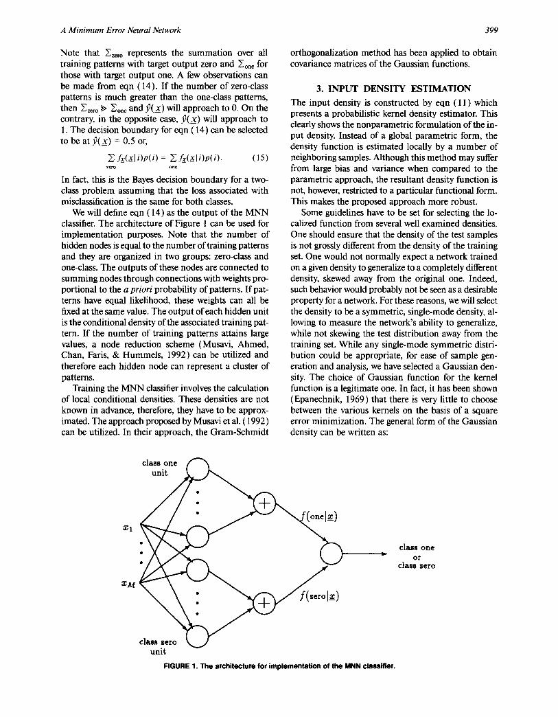
We will define eqn (14) as the output of the MNN classifier. The architecture of Figure 1 can be used for implementation purposes. Note that the number of hidden nodes is equal to the number of training patterns and they are organized in two groups: zero-class and one-class. The outputs of these nodes are connected to summing nodes through connections with weights proportional to the a priori probability of patterns. If patterns have equal likelihood, these weights can all be fixed at the same value. The output of each hidden unit is the conditional density of the associated training pattern. If the number of training patterns attains large values, a node reduction scheme (Musavi, Ahmed, Chan, Faris, & Hummels, 1992) can be utilized and therefore each hidden node can represent a cluster of patterns.

Training the MNN classifier involves the calculation of local conditional densities. These densities are not known in advance, therefore, they have to be approx- imated. The approach proposed by Musavi et al. (1992) can be utilized. In their approach, the Gram-Schmidt

orthogonalization method has been applied to obtain covariance matrices of the Gaussian functions.

3. INPUT DENSITY ESTIMATION

The input density is constructed by eqn (11 ) which presents a probabilistic kernel density estimator. This clearly shows the nonparametric formulation of the input density. Instead of a global parametric form, the density function is estimated locally by a number of neighboring samples. Although this method may suffer from large bias and variance when compared to the parametric approach, the resultant density function is not, however, restricted to a particular functional form. This makes the proposed approach more robust.

Some guidelines have to be set for selecting the lo- calized function from several well examined densities. One should ensure that the density of the test samples is not grossly different from the density of the training set. One would not normally expect a network trained on a given density to generalize to a completely different density, skewed away from the original one. Indeed, such behavior would probably not be seen as a desirable property for a network. For these reasons, we will select the density to be a symmetric, single-mode density, allowing to measure the network's ability to generalize, while not skewing the test distribution away from the training set. While any single-mode symmetric distribution could be appropriate, for ease of sample generation and analysis, we have selected a Gaussian density. The choice of Gaussian function for the kernel function is a legitimate one. In fact, it has been shown (Epanechnik, 1969) that there is very little to choose between the various kernels on the basis of a square error minimization. The general form of the Gaussian density can be written as:

class one t / ~

@

XM

class zero ~ , / unit

FIGURE 1. The architecture for implementation of the MNN classifier.

class one o r

class zero

400

f x(_x]i) = (2~r)-M/z]z~]-'/2exp(-½dZ~(x_)), (16)

where Y.i is the covariance matrix, and d~(__x) is defined a s :

d2(x) = ( x - s ' i )T[~]-~(x- si). (17)

The conditional density will peak when the corresponding training pattern s g is presented at the input.

3.1. Parameter Estimation

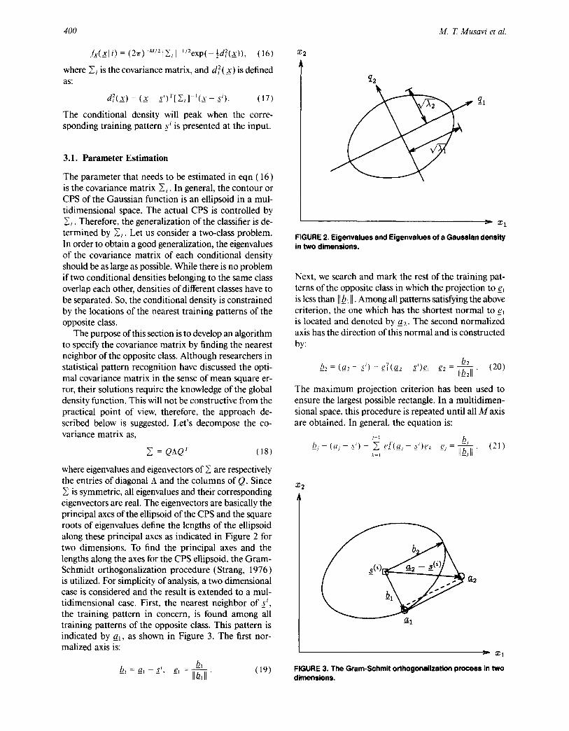
The parameter that needs to be estimated in eqn (16) is the covariance matrix ~i . In general, the contour or CPS of the Gaussian function is an ellipsoid in a mul- tidimensional space. The actual CPS is controlled by ~i. Therefore, the generalization of the classifier is determined by ~ . Let us consider a two-class problem. In order to obtain a good generalization, the eigenvalues of the covariance matrix of each conditional density should be as large as possible. While there is no problem if two conditional densities belonging to the same class overlap each other, densities of different classes have to be separated. So, the conditional density is constrained by the locations of the nearest training patterns of the opposite class.

The purpose of this section is to develop an algorithm to specify the covariance matrix by finding the nearest neighbor of the opposite class. Although researchers in statistical pattern recognition have discussed the optimal covariance matrix in the sense of mean square error, their solutions require the knowledge of the global density function. This will not be constructive from the practical point of view, therefore, the approach de- scribed below is suggested. Let's decompose the covariance matrix as,

= QAQ T ( 1 8 )

where eigenvalues and eigenvectors of ~ are respectively the entries of diagonal A and the columns of Q. Since

is symmetric, all eigenvalues and their corresponding eigenvectors are real. The eigenvectors are basically the principal axes of the ellipsoid of the CPS and the square roots of eigenvalues define the lengths of the ellipsoid along these principal axes as indicated in Figure 2 for two dimensions. To find the principal axes and the lengths along the axes for the CPS ellipsoid, the Gram- Schmidt orthogonalization procedure (Strang, 1976) is utilized. For simplicity of analysis, a two dimensional case is considered and the result is extended to a mul- tidimensional case. First, the nearest neighbor of s i, the training pattern in concern, is found among all training patterns of the opposite class. This pattern is indicated by a~, as shown in Figure 3. The first normalized axis is:

bl ~l = a , - - S i, e I - I I_b, II " ( 1 9 )

-~2

- q l

M. T Musavi et aL

X2

X 1

FIGURE 2. Eigenvslues and Eigenvelues of a Gaussian density in two dimensions.

Next, we search and mark the rest of the training patterns of the opposite class in which the projection to _el is less than ]lb~ []. Among all patterns satisfying the above criterion, the one which has the shortest normal to _e~ is located and denoted by _a2. The second normalized axis has the direction of this normal and is constructed by:

b2 h 2 = (_a2 - s ' ) - d ( _ a _ 2 - _s ' ) ¢ , _e2 = I I h ~ l l " ( 2 0 )

The maximum projection criterion has been used to ensure the largest possible rectangle. In a multidimen- sional space, this procedure is repeated until all M axis are obtained. In general, the equation is:

i1 b j (21) h , - ( a , - g ) - Z ¢ [ ( _a , - g ) ¢ k e j -- II_bjll " k=l

X2

..~z I

~-- X 1

FIGURE 3. The Grsm-Schmit orthogonalization process in two dimensions.


X

., " ~ class A ,. ,, ,, " "*" ~ boundary

., ,,, "" f %

",, V ". , \ ,, .....

" "1, 1 d=.B ~ o ,- k" , / I boundary

i , , " ~ _ J l

X 1

FIGURE 4. Separation of decision regions.

Note that the selected aj, as in ~2, should meet the projection criteria for all ( j - 1 ) eigenvectors. This can be expressed as:

t_eT(aj-s')l < II_bkll for k = 1, 2 . . . . . j - 1. (22)

Therefore, the number of patterns searched decreases as j increases. If there is no more point satisfying these criteria, bj will not be constrained in a particular direction. The only requirement is that it should be orthogonal to the previously constructed axes and Ilbll can be set at a predefined maximum value or equal to the length of the previous axis. Note that II_bj II cannot be zero since this means that such a vector is linearly dependent to other axes. If such a case arises, the selected nearest neighbor is aborted and the second nearest one will be substituted.

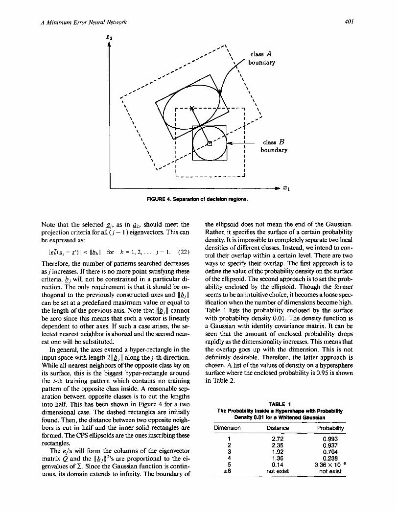
In general, the axes extend a hyper-rectangle in the input space with length 2 Ilbjll along the j - th direction. While all nearest neighbors of the opposite class lay on its surface, this is the biggest hyper-rectangle around the i-th training pattern which contains no training pattern of the opposite class inside. A reasonable separation between opposite classes is to cut the lengths into half. This has been shown in Figure 4 for a two dimensional case. The dashed rectangles are initially found. Then, the distance between two opposite neighbors is cut in half and the inner solid rectangles are formed. The CPS ellipsoids are the ones inscribing these rectangles.

The _ej's will form the columns of the eigenvector matrix Q and the Ilbjll 2's are proportional to the eigenvalues of ~. Since the Gaussian function is contin- uous, its domain extends to infinity. The boundary of

the ellipsoid does not mean the end of the Gaussian. Rather, it specifies the surface of a certain probability density. It is impossible to completely separate two local densities of different classes. Instead, we intend to con- trol their overlap within a certain level. There are two ways to specify their overlap. The first approach is to define the value of the probability density on the surface of the ellipsoid. The second approach is to set the probability enclosed by the ellipsoid. Though the former seems to be an intuitive choice, it becomes a loose spec- ification when the number of dimensions become high. Table 1 lists the probability enclosed by the surface with probability density 0.01. The density function is a Gaussian with identity covariance matrix. It can be seen that the amount of enclosed probability drops rapidly as the dimensionality increases. This means that the overlap goes up with the dimension. This is not definitely desirable. Therefore, the latter approach is chosen. A list of the values of density on a hypersphere surface where the enclosed probability is 0.95 is shown in Table 2.

TABLE 1 The Probability Inside a Hyperahape with Probability

Density 0.01 for a Whitened Gaussian

Dimension Distance Probability

1 2.72 0.993 2 2.35 0.937 3 1.92 0.704 4 1.36 0.238 5 0.14 3.36 × 10 -6

->6 not exist not exist

402

TABLE 2 The Values of Density on a Hypersphere Where the

Enclosed Probability is 0.95 for a Whitened Gaussian

Dimension Distance Density

1 1.96 5.84 × 10 -2 2 2.45 7.96 × 10 -3 3 2.80 1.28 × 10 3 4 3.08 2.21 × 10 4 5 3.33 3.98 × 10 -s 6 3.55 7.43 × 10 -s 7 3.75 1.42 × 10 s 8 3.94 2.75 × 10 -7 9 4.11 5.43 x 10 -8

10 4.28 1.08 × 10 -8

M. T. Musav i et hi.

TABLE 3 The Values of r 2 When V is 0.9545

M r 2

1 4.000 2 6.180 3 8.025 4 9.716 5 11.32 6 12.85 7 14.34 8 15.79 9 17.21

10 18.61

In order to simplify the discussion, let's start from a whitened Gaussianfw(x) with zero mean and identity covariance matrix. After a whitening transform de- scribed in eqn (23), an ellipsoid can be converted to a unit hypersphere.

y_ = A I / 2 Q r x = ( Q A - l / 2 ) r x . (23)

NOW let's define a radius r such that the probability enclosed by the hypersphere with radius r is v. This can be expressed as:

fw(x_)dx_ v < v < (24) where 0 1. _x112~r 2

Since the covariance matrix of this Gaussian is fixed, the corresponding r can be determined for any given probability v. Let's define R 2 = [[ x[[ 2 that can be shown to have a Chi-square distribution (Papoulis, 1984). Then v can be expressed as:

1 ~ r2/2 - - - Z ( ' + M / 2 ) e - Z d z (25) V = P ( R 2 < r 2) P(M/2) oo

where P(. ) is the Gamma-function. This integration can be evaluated by numerical techniques. Figure 5 shows the relationship between v and r for several values of M. In particular, Table 3 lists the values of r E for up to l0 dimensions when v is fixed at 0.9545. This number is selected for the experiments reported in this paper because it specifies a small amount of overlap and r E

is 4.0 in a one-dimensional case. It is expected that the [I bj I[/2's constrain the ellipsoid

as r constrains the hypersphere. In fact, they are related by eqn (23). Substitute b j /2 for _x in eqn (23). Since _bj is orthogonal to all the eigenvectors except e j , Q r b i /

2 ends up with a vector having zeros in all its components except the j-th, which is [[bi[[/2. On the left hand side, y should be in the direction of the j - th axis of the hypersphere with a magnitude r. That is,

Ill ! M = I ~

0.8 . . . . . . . . . . . . . . . . . . . . . . . . . . . . . . . . . . . . . . . . . . . . . . . . . . . . . . . . . . . . . . . . . . . . . . . .

=. 0.6 . . . . . . . . . . .

O.4o.z .... i ............ . . . . . . . . . . .

o 0 1 2 3 4 5 6

FIGURE 5. The probability versus the radius of the hypersphere.


r = ~ ' /2 Ilbjll (26) 2

Therefore, the eigenvalues can be found from:

Ilbjll (27) ~ j - 4 r 2 .

Once eigenvalues and eigenvectors are known, the conditional densities f_x(_Xl i) can be evaluated, and this concludes our discussion.

3.2. Numerical Integration

The evaluation algorithm proposed here requires mul- tidimensional integration. Unfortunately, it is not always possible to obtain such an integral by an analytical approach, even if the conditional densities are as simple as Gaussian. In other words, a closed form expression for the classifier performance is not always available. Furthermore, in order to keep this algorithm more robust, there should not be any restriction on the functional form of the error function. Therefore, a suitable approach is a numerical integration technique.

The Monte Carlo method is the simplest, if not the most feasible, approach for numerical integration in higher order dimensions. This technique has been selected in our experiments due to the following reasons. First, no particular functional form is expected for the integrand. Second, the complicated transforms, if they exist, are basically avoided. Third, the number of random points required to obtain a certain precision is independent of the number of dimensions (not nec- essarily true for pseudorandom numbers).

4. MNN vs PNN

There are similarities between the MNN presented here and the PNN presented by Specht. Both of these networks use kernel estimators, follow the Bayes decision boundary, have simple architecture, and are time efficient. The MNN, however, offers a few nice features that have resulted in a better error rate, even with low number of training patterns. The MNN decision boundary is based on many covariance matrices while the PNN uses only one single covariance matrix (i.e., proportional to identity, ~ = aI) for all kernel nodes. In MNN, the Gram-Schmidt orthogonalization process is used to find a set of covariance matrices while in PNN the smoothing parameter is found by trial and measurement of error on the training set using the holdout method. In contrast, PNN requires only one memory location for the smoothing parameter while MNN requires a storage capacity of T M 2 in which T is the total number of training patterns and M is the dimension of the input space. Also, calculation of many covariance matrices is more time consuming than se-

lecting a value for smoothing parameter. Therefore, a better performance is achieved at the expense of memory and speed of training. However, these disadvantages of MNN are subdued by the fact that fewer training points are required by MNN to achieve a level of generalization that requires many training data with the PNN. It should also be noted that a clustering algorithm (Musavi, Ahmed, Chan, Faris, & Hummels, 1992 ) can be applied to the training samples in order to reduce the number of covariance matrices.

In order to compare the generalization ability of MNN and PNN, we first investigate the differences between their decision boundaries and show how radically the PNN decision boundary might change with the smoothing parameter. While any problem with any number of training patterns, dimensions, and classes could have been used here, for the sake of simplicity and graphical display of the boundaries, we selected a two-class, two-dimensional example, as shown in Figure 6. Seventeen patterns of class "O" and " × " were generated by Laplace densities and used as training data. Different values of smoothing parameter tr were selected and for each one the PNN classifier was tested with 10,000 samples of the given distributions. The best performance which yielded 21.7% error rate was recorded to be at a = 0.02. The decision boundary for this tr is presented in Figure 6 with a dotted line. To show the sensitivity of the PNN with respect to a, two other decision boundaries for a = 0.01 and 0.5 have been also presented in Figure 6 with dotted lines. The changes in the decision boundaries due to different values of a are significant and this explains why for a q: 0.02 the error rate is higher.

Using the same training points, a MNN classifier was built and tested with the same number of test patterns. An error rate of 12.5% was recorded as compared to 21.7%. Note that for the given problem the MNN used 17 covariance matrices, one for every training pattern. The decision boundary for the MNN is also shown in Figure 6 with solid line. The differences between decision boundaries are clearly shown in Figure 6. The error rate of the MNN classifier for the given problem was much better than the optimal performance of the PNN classifier. Other tests have been also con- ducted and reported in the following section to verify the improved performance of the MNN network.

5. TEST RESULTS

Two test problems with two (2-d) and eight (8-d) input dimensions have been selected to show the results in low and high dimensions. Without loss of generality it has been assumed that there are only two classes in each problem. The 2-d problem was generated by Gaussian random vectors. The first class has zero mean


C~ X

0.5

0 . 4

0.3

0.2

0 . I

0

- 0 . I

- 0 . 2

- 0 . 3

0 . 5 - 0 . 4

- 0 . 5 - 0 . 8

i

PNN .....

MNN

i

- 0 . 6 - 0 . 4

i t," i ~ i

/

X / i "

• :" 0

X x x o

l °° o o.02

o . . . . . . . . . . . . . . . . . . . . . . . . . . . . . . . . . . . .

x ..... .... . 0.1 MN,N - 0 . 2 0 0.2 0.4

X1

FIGURE 6. Dec i s i on boundaries for the MNN and PNN.

random vectors with identity covariance matrix and the second class has a mean vector [ 1 2 ] and a diagonal covariance matrix with 0.01 and 4.0 entries. The distribution of training samples for this problem is shown

in Figure 7. The pattern of the first class has been indicated by " × " and the second class by dots ".". The patterns of the 8-d problem are also Gaussian random vectors with equal mean vectors and identity ( I ) and

6

4

2

0

-2

-4 -3

x x

xx x x

x x

x

x

I

-2

X X

X

X

• • ,o..." °.

. . , . .

• . . . : , •

. , : , : o . , . . . . o .

x x

x "<:.X x x x " , :~.f~. x x x x

3. x x ~ X _, x x "~:~L"" ,.~x X r x ~ T x x , . ...~ x x

x _ x x ~ x ~ ~ ' ~ X . A _ _ ] ( - ~ - " X X ~: .~ •

x x t x" xx x ~'x . . . ' . x x x ~ x x ~ xx x x

x x x xXX% Xx xx x:X~k" X X X X

X X X X X

X

X X

I i I I

- I 0 1 2

FIGURE 7. The training samples of the 2-d probiem.


Error%

2O 19 18 17 16 ]5

13 ]2 11

9 8 7 6 ~ 5

= 100

$ 150

: 200 ; 250 : 300

. . . . ;:3 --- "1

4 I I l I I I I I " ( ~

0 .05 0.1 0 .15 0.2 0 .4 0 .6 0.8 1.0

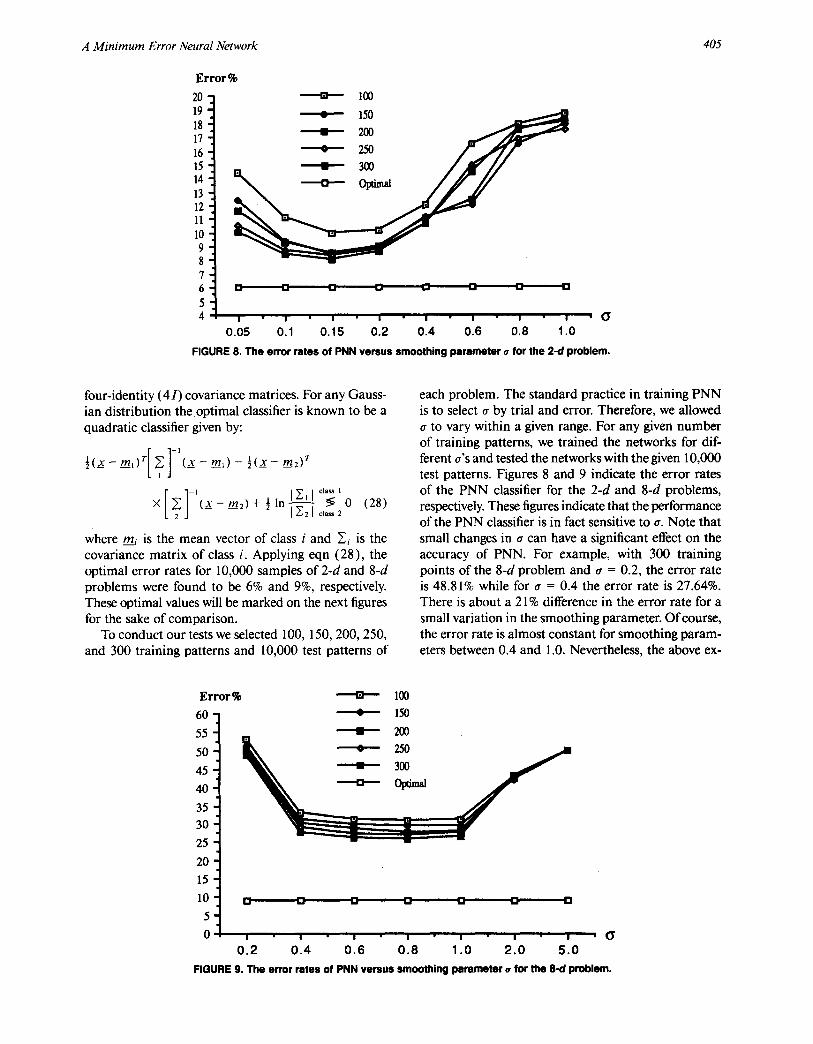
FIGURE 8. The error rates of PNN versus smoothing parameter ¢ for the 2-d problem.

four-identity (4 I) covariance matrices. For any Gauss- ian distribution the optimal classifier is known to be a quadratic classifier given by:

l( ._X - - FF/I) T ( X - - _m_ml) - - l ( x - - ~ m 2 ) T

X 0 (28) × ( x - m2) + ½ In ~ ~,~2

where rni is the mean vector of class i and Y.i is the covariance matrix of class i. Applying eqn (28), the optimal error rates for 10,000 samples of 2-d and 8-d problems were found to be 6% and 9%, respectively. These optimal values will be marked on the next figures for the sake of comparison.

To conduct our tests we selected 100, 150, 200, 250, and 300 training patterns and 10,000 test patterns of

each problem. The standard practice in training PNN is to select ~ by trial and error. Therefore, we allowed

to vary within a given range. For any given number of training patterns, we trained the networks for different a's and tested the networks with the given 10,000 test patterns. Figures 8 and 9 indicate the error rates of the PNN classifier for the 2-d and 8-d problems, respectively. These figures indicate that the performance of the PNN classifier is in fact sensitive to a. Note that small changes in tr can have a significant effect on the accuracy of PNN. For example, with 300 training points of the 8-d problem and ~ = 0.2, the error rate is 48.81% while for a = 0.4 the error rate is 27.64%. There is about a 21% difference in the error rate for a small variation in the smoothing parameter. Of course, the error rate is almost constant for smoothing parameters between 0.4 and 1.0. Nevertheless, the above ex-

Error% ~ I00

60 ~. 150

55 -- 200

50 ° 250 i = 45 - 3oo.

35 30

25

20

15

0 ~ 0 . 2 0 . 4 0 . 6 0 . 8 1 . 0 2 . 0 5 . 0

FIGURE 9. The error rates of PNN versus smoothing parameter o for the 8-d problem.


Error % 12

10

a - - - p ~

L

I m b [] . . • .

Training data I I I I I

100 150 200 250 300

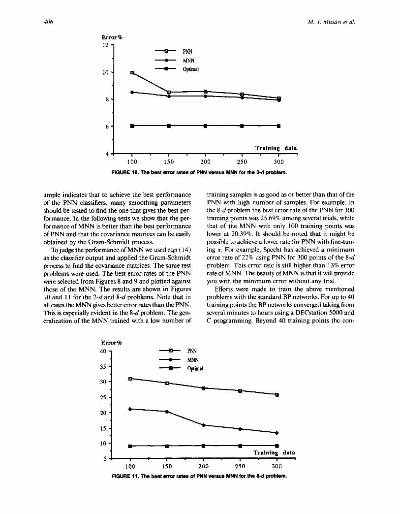
FIGURE 10. The best error rates of PNN versus MNN for the 2-d problem.

ample indicates that to achieve the best performance of the PNN classifiers, many smoothing parameters should be tested to find the one that gives the best performance. In the following tests we show that the performance of MNN is better than the best performance of PNN and that the covariance matrices can be easily obtained by the Gram-Schmidt process.

To judge the performance of MNN we used eqn (14) as the classifier output and applied the Gram-Schmidt process to find the covariance matrices. The same test problems were used. The best error rates of the PNN were selected from Figures 8 and 9 and plotted against those of the MNN. The results are shown in Figures l0 and I 1 for the 2-d and 8-d problems. Note that in all cases the MNN gives better error rates than the PNN. This is especially evident in the 8-d problem. The generalization of the MNN trained with a low number of

training samples is as good as or better than that of the PNN with high number of samples. For example, in the 8-d problem the best error rate of the PNN for 300 training points was 25.69% among several trials, while that of the MNN with only 100 training points was lower at 20.39%. It should be noted that it might be possible to achieve a lower rate for PNN with fine-tun- ing ~. For example, Specht has achieved a minimum error rate of 22% using PNN for 300 points of the 8-d problem. This error rate is still higher than 13% error rate of MNN. The beauty of MNN is that it will provide you with the minimum error without any trial.

Efforts were made to train the above mentioned problems with the standard BP networks. For up to 40 training points the BP networks converged taking from several minutes to hours using a DECstation 5000 and C programming. Beyond 40 training points the con-

Error% 40

35

30

25

20

15

10

5

m--- PNN

~. MNN

v

m m m m

Training data

100 150 200 250 300

FIGURE 11. The best error rates of PNN versus MNN for the 8-d problem.


vergence was almost impossible regardless of the number of layers and nodes. In contrast, all MNN networks performed under 10 minutes. It is also important to note that in the converged BP networks, the error rates were higher than MNN.

6. CONCLUSION

A MNN has been presented, which has been shown to offer better error rates than PNN and BP networks. The distinction lies in the fact that many covariance matrices, as opposed to only one, are used to subdivide the input space into different regions. The architecture for the MNN is similar to that of PNN, however, it requires more memory to store covariance matrices.

REFERENCES

Epanechnik, V. A. (1969). Nonparametric estimation of a multidi- mensional probability density. Theory of Probability Application, 14, 153-158.

Maloney, E S., & Specht, D. E (1989). The use ofprobabilistic neural networks to improve solution times for hull-to-emitter correlation problems. Proceedings of International Joint Conference on Neural Networks, San Diego, CA, 1, 289-294.

Montana, D. ( 1991 ). A weighted probabilistic neural network. Ad- vances in Neural Information Processing Systems, 4, I 110-1117.

Musavi, M. T., Ahmed, W., Chan, K. H., Faris, K., & Hummels, D. M. ( i 992). On the training of radial basis function classifiers. Neural Networks, 5(4), 595-603.

Papoulis, A. (1984). Probability, random variables, and stochastic processes. New York: McGraw-Hill.

Specht, D. E (1967). Generation of polynomial discriminant functions for pattern recognition. IEEE Transactions on Electronic Computer, EC-16, 308-319.

Specht, D. E (1990a). Probabilistic neural networks. NeuralNetworks, 3(1), 109-118.

Specht, D. E (1990b). Probabilistic neural networks and the polynomial adaline as complementary techniques for classification. I EEE Transactions on Neural Networks, 1 ( I ), 111-121.

Specht, D. E (1991). A general regression neural network. IEEE Transactions of Neural Networks, 2(6), 568-576.

Specht, D. E, & Shapiro, P. D. ( 1991 ). Generalization accuracy of probabilistic neural networks compared with back propagation networks. Proceedings of International Joint Conference on Neural Networks, Seattle, WA, I, 887-892.

Strang, G. (1976). Linear algebra and its applications. New York: Academic Press.

Washburne, 1". P., Okamura, M. M., Specht, D. E, & Fisher, W. A. (1991). The Lockheed probabilistic neural network processor. Proceedings of International Joint Conference on Neural Networks, Seattle, WA, I, 513-518.

Yoshimoto, S. (1990). A study on artificial neural network generalization capability. Proceedings of lnternational Joint Conference on Neural Networks, San Diego, CA, III, 689-694.

A minimum error neural network (MNN

Documents

Transcript of A minimum error neural network (MNN