A method for climatic reconstruction of the Mediterranean Pliocene using pollen data

ELSEVIER Palaeogeography, Palaeoclimatology, Palaeoecology 144 (1998) 183–201

A method for climatic reconstruction of the Mediterranean Plioceneusing pollen data

Severine Fauquette a,Ł, Joel Guiot a, Jean-Pierre Suc b

a Institut Mediterraneen d’Ecologie et de Paleoecologie (ERS CNRS 6100), case 451, Faculte des Sciences de Saint-Jerome, AvenueEscadrille Normandie-Niemen, 13297 Marseille cedex 20, France

b Centre de Paleontologie stratigraphique et Paleoecologie (UMR CNRS 5565), Universite Claude Bernard, Lyon 1,29 boulevard du 11 Novembre, 69622 Villeurbanne cedex, France

Received 25 November 1997; accepted 27 May 1998

Abstract

Pollen data from numerous sites around the Mediterranean Sea indicate that several important vegetation and climaticchanges occurred during the Pliocene. These data are in good agreement with pollen records from northwest Europeand with Ž18O curves from Mediterranean and Atlantic deep-sea cores. Quantitative palaeoclimatic reconstructions fromPliocene pollen data of the Mediterranean region cannot be based on conventional modern analogue techniques, asindividual Pliocene pollen spectra contain taxa representing temperate, warm-temperate and subtropical plants that do notgrow together today. Instead, we propose a new method that uses a climatic amplitude method modified to take partiallyinto account the relative abundances of the taxa. We applied this method to the Pliocene Garraf 1 palynological sequencefrom Catalonia, which provides a long continuous record of climatic change from 5.3 Ma to the Early Pleistocene. Weestimate that annual temperatures were 1 to 5ºC higher than today and the annual precipitation 400 to 1000 mm higherthan today prior to the beginning of the late Cenozoic glacial–interglacial cycles. In contrast, temperature and precipitationboth fell sharply during the glacial phases of the earliest glacial–interglacial cycles. 1998 Elsevier Science B.V. Allrights reserved.

Keywords: climatic reconstruction; climate tolerance of plants; Pliocene; Mediterranean region; pollen

1. Introduction

During the Pliocene mid-latitude environmentschanged from tropical and subtropical to near-mod-ern conditions (Zagwijn, 1960; Axelrod, 1973; Suc,1984; Pons et al., 1995). This period is particularlywell-documented in pollen records from western andsouthern Europe. The Mediterranean and nearby re-

Ł Corresponding author. Tel.: C33 (491) 288524; Fax: C33 (491)288668; E-mail: [email protected]

gions provide several continuous Pliocene pollensequences (Cravatte and Suc, 1981; Suc and Cra-vatte, 1982; Bessais and Cravatte, 1988; Drivaliari,1993; Bertini, 1994; Drivaliari et al., 1998). Themain climatic events identified using pollen recordsare fully consistent with those defined using the Ž18Odeep-sea records (Tiedemann et al., 1994; Shack-leton et al., 1995) and also Mediterranean Ž18Orecords (Vergnaud Grazzini et al., 1990; Thunell etal., 1990). In addition to their variability in time,Mediterranean Pliocene pollen diagrams show a high

0031-0182/98/$19.00 c 1998 Elsevier Science B.V. All rights reserved.PII: S 0 0 3 1 - 0 1 8 2 ( 9 8 ) 0 0 0 8 3 - 2

184 S. Fauquette et al. / Palaeogeography, Palaeoclimatology, Palaeoecology 144 (1998) 183–201

degree of spatial variability (Suc, 1989; Suc et al.,1995a), and the overall geographic pattern is moreor less similar to the modern pattern (Suc et al.,1995a,b). Consequently, the area appears very pro-pitious to Pliocene climatic quantification with theaim of testing general circulation models such asthe GISS model which has been run for this period(Crowley, 1991; Chandler et al., 1994). Dowsett etal. (1992) have emphasised the importance of thelast Pliocene climatic warming at 3.1 Ma before theonset of glacial–interglacial cycles (at 2.6 Ma) forproviding insights into possible future climatic con-ditions under a warmer-than-modern ‘greenhouse’climate. This middle Pliocene warm period is welldocumented in the Mediterranean region.

Pliocene pollen spectra from the Mediterraneanregion include many taxa still extant in Europeand the circum-Mediterranean areas (for example,Quercus, Olea, Cistus), in addition to subtropicalelements (for example, Taxodiaceae, Engelhardia,Symplocos) that no longer live in these regions.These combinations of pollen taxa cannot be foundoccurring together in the modern landscape, thusprecluding the use of the best analogue method forclimatic reconstruction (Guiot, 1990). Consequently,it is necessary to devise an alternative method, whichdoes not need any analogue, to reconstruct the cli-mate of this period. The method proposed here usesthe climatic requirements of a few modern taxa tointerpret the fossil data. Although other researchershave attempted similar studies (Zagwijn, 1975; Mai,1995; Suc et al., 1995b), this is the first large-scalesystematic attempt to reconstruct Pliocene climatesfrom modern floral vegetation=climate relations.

Our method involves two steps: (1) determinationof the precise climatic ranges of a few key plantsof the Mediterranean Pliocene, including both ex-tirpated subtropical plants and plants that still livein the region (Fauquette et al., 1998a), and (2) de-termination of the climatic amplitudes of variouspollen-taxa on the basis of several thousand pollenmodern spectra. In contrast with the best analoguemethod (Guiot, 1990), this approach does not rely onthe analysis of entire pollen assemblages, but ratheron interpreting the pollen abundance of each indi-vidual taxon in relation to climate. Such a type ofmethod was developed by Iversen (1944) to quan-tify the post-glacial climate from a few indicator

plant species and by Atkinson et al. (1986), whotook their inspiration from Grichuk (1969), to quan-tify the palaeoclimatic interpretations of Quaternarycoleoptera. These last authors called the method the‘Mutual Climatic Range Method’ that is based onthe establishment of the range of climates occupiedat the present-day by beetle species represented in afossil assemblage.

Here, we present first the full description of thisnew quantitative pollen-derived palaeoclimatic re-construction. In a second part, we present its appli-cation to a Pliocene marine pollen record (Garraf 1core, Suc and Cravatte, 1982). The palaeoclimatic in-terpretations from this core are then compared withthe climatic changes seen in deep-sea Ž18O curves(Thunell et al., 1990; Vergnaud Grazzini et al., 1990;Tiedemann et al., 1994) and to the values obtainedby transfer functions based on marine (Dowsett andPoore, 1991; Edwards et al., 1991) or continental(Montuire, 1994; Michaux et al., 1996; Aguilar etal., 1998) faunas.

2. Modern data and method

2.1. Taxa still living in Europe and in theMediterranean region

Almost 8000 modern pollen spectra were usedin the statistical part of the method. These spectracorrespond to surface samples or core-tops whichwere collected in the Northern hemisphere, in Eura-sia and in North America and then compiled by B.Huntley, P.J. Bartlein, (pers. commun.) and Peyronet al. (1998). They represent a great diversity of veg-etation and sedimentary environment types, and thusof climates. These modern pollen spectra allow usto include in our analysis a range of climates fromnorthern boreal to warm-temperate conditions.

The values of the modern climatic parameterscorresponding to each sampling site have been pro-vided by B. Huntley (pers. commun.) according tothe following procedure: (1) mean monthly values,of temperature, precipitation and cloudiness wereinterpolated using Laplacian thin-plate spline sur-faces (Hutchinson, 1989), (2) bioclimatic variables[temperatures of the coldest and warmest months,E=PE (the ratio of actual evapotranspiration to po-

S. Fauquette et al. / Palaeogeography, Palaeoclimatology, Palaeoecology 144 (1998) 183–201 185

tential evapotranspiration), GDD5 (growing degree-days above 5ºC)] were calculated with the biome 1model of Prentice et al. (1992), using the monthlyinterpolated meteorological values.

Pollen percentages were calculated for each spec-trum, based on the total pollen sum, but excludingpollen of water-plants and spores. Cyperaceae pollenis included in the pollen sum.

Six climatic parameters were considered: meanannual temperature .TA/, total annual precipitation.PA/, mean temperature of the coldest month .TC/,mean temperature of the warmest month .TW/, avail-able moisture (i.e. the ratio of actual evapotranspi-

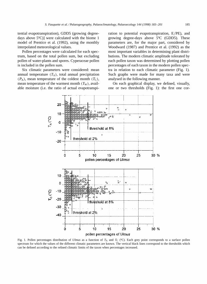
Fig. 1. Pollen percentages distribution of Ulmus as a function of TA and TC (ºC). Each grey point corresponds to a surface pollenspectrum for which the values of the different climatic parameters are known. The vertical black lines correspond to the thresholds whichcan be defined according to the refined climatic limits of the taxon when percentages increased.

ration to potential evapotranspiration, E=PE), andgrowing degree-days above 5ºC (GDD5). Theseparameters are, for the major part, considered byWoodward (1987) and Prentice et al. (1992) as themost important variables in determining plant distri-butions. The modern climatic amplitude tolerated byeach pollen taxon was determined by plotting pollenpercentages of each taxon in the modern pollen spec-tra in relation to each climatic parameter (Fig. 1).Such graphs were made for many taxa and wereanalysed in the following manner.

On each graphical display, we defined, visually,one or two thresholds (Fig. 1): the first one cor-


responds to the presence=absence threshold underwhich the taxon is probably not at the site (pollenpercentages below this level reflect long-distancetransport by wind or water); the second one cor-responds to the abundance threshold. Sometimes athird threshold is defined, reducing again the ampli-tude of almost one of the parameters. Each of thesethresholds are taxon-dependent and may be differentfor each taxon. In a given pollen spectrum (mod-ern or fossil), if the percentage of a taxon exceeds80% of the first (lower) threshold, then the climaticamplitude associated with that threshold is used inthe reconstruction. If the percentage of the taxon ex-ceeds 80% of the second (upper) threshold, then themore restricted climatic amplitude associated withthat threshold is used also. Values of TC, TW, GDD5and available moisture have been homogenised withthose given by Prentice et al. (1992) according tothe plant functional type. For example, the minimumtolerated value of available moisture of sclerophyllplants corresponds to 28% (Prentice et al., 1992).

Of course, the so-obtained climatic ranges arenot real physiological values. The obtained valuesdepend in part on the method used to define theintervals and also on the diversity of the modern dataset. The way of determination of the climatic condi-tions tolerated by these plants, based on pollen data,does not allow to consider the extreme cases of en-durance of the plants, because modern pollen spectrahave not been collected from all parts of the earth.

For the calculation of palaeoclimatic estimatesfor low and middle-low altitude Pliocene sites, thepollen taxa have been separated into three groups:a group (U) of ubiquitous (at the genus level) taxa(for example Quercus deciduous type); a group (C)of taxa growing in cold regions (at high altitudesand=or high latitudes, for example Picea, Abies etc.);a third group (W) of taxa growing in warm regions(at low altitudes and=or low latitudes, for exampleArbutus, Quercus evergreen type, Zizyphus etc.). Forpollen taxa such as Poaceae and Cyperaceae forwhich we cannot determine the species or even thegenus, two climatic ranges have been defined on thegraphs, one for taxa growing in cold regions and asecond for taxa growing in warm regions.

All these values (thresholds, groups and climaticamplitudes) are given in Table 1 which provides thekey data for climate reconstructions. For a given

spectrum, each taxon exceeding its threshold(s) pro-vides a climatic range which was compared to thoseobtained for the other taxa. The most probable cli-matic range for the spectrum was provided by thesmallest climatic range suitable for the maximumof taxa (i.e. the likely interval [R�; RC]) (Fig. 2).If the reconstructed climatic interval was too small(i.e. less than 5% of the maximum climatic range)and thus had a low level of probability, the lowerand upper limits were extended to the next smallerinterval (i.e. the enlarged interval [R0�; R0C]).

For each Pliocene sample, two different his-tograms were considered: one with ubiquitous andcold plants (high altitude) and another with ubiqui-tous and warm plants (low altitude). We then calcu-lated a ‘most likely value’ which corresponded to aweighted mean in relation to the inverse of the ex-ternal surface of the histogram (below R� and aboveRC):

R0 DR�SIC RC

SS1

SIC 1

SS

where R� is the lower limit of the likely interval, RCis the upper limit, SI the inferior surface (below R�),SS the superior surface (above RC) (Fig. 2). We im-posed two conditions: R0 was necessarily includedin the likely interval, and in the case where the inter-val has been enlarged to the lower probability level(between R0� and R0C, Fig. 2), R0 was constrained tobe in the restricted interval [R0�; R0C].

This way of calculation allows us to give moreweight to the subtropical taxa when they are rela-tively numerous, as in the case of subtropical fossilspectra. A small external surface gives more pre-cise information concerning the limits of the climaticranges, whereas a large external surface implies aprobable mixture of non-compatible pollen taxa in asingle assemblage.

2.2. Marker-taxa of the Mediterranean Pliocene

Some important ‘marker’-taxa cannot be studiedin the same way because of the lack of modernsubtropical pollen spectra that contain the Pliocenepollen taxa. Instead, we estimated the modern cli-matic ranges of subtropical taxa by examining their


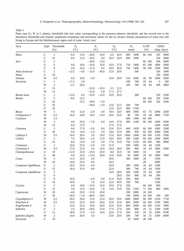
Table 1Plant type (U, W or C plants), thresholds (the first value corresponding to the presence=absence threshold, and the second one to theabundance threshold) and climatic amplitudes (minimum and maximum values for the six chosen climatic parameters) of some taxa stillliving in Europe and the Mediterranean region and of some ‘exotic taxa’

Taxa Type Thresholds TA TC TW PA E=PE GDD5(%) (ºC) (ºC) (ºC) (mm) (%) (degr. days)

Abies C 5 �6.0 13.0 �20.0 10.0 6.0 26.0 600 1600 66 100 350 3000C 25 0.0 11.0 �16.0 4.0 10.0 24.0 600 1600 350 3000

Acer U 2 �20.0 13.0 66 100 500 5600U 6 0.0 18.0 �16.0 10.0 16.0 27.0 750 1400 85 100 1000 5000U 8 4.0 16.0 �11.0 6.0 18.0 26.0 750 1400 90 100 1500 3900

Alnus fruticosa C 2 �12.5 �4.0 �35.0 �30.0 12.0 20.0 500 350 1000Alnus U 10 350 4200Arbutus W 0.5 8.0 18.0 �5.0 19.0 26.0 550 1600 28 90 1000 5000Artemisia C 5 �17.5 5.0 100 700 18 64 0 500

W 5 �2.5 20.0 100 700 18 64 500 5800C 15 �35.0 �25.0 2.5 12.5W 15 �25.0 5.0 17.5 27.5

Betula nana C 2 �13.0 0.0 �35.0 �12.0 10.0 20.0 500 350 1500Betula U 5 �8.0 12.5 66 100 350 2500

U 25 12.5 �30.0 �5.0 66 100 350 2500U 35 �30.0 �5.0 12.0 22.5 200 700U 35 12.0 22.5 900 1700

Buxus W 3 9.0 12.0 �2.0 4.0 18.0 24.0 600 1000 65 75 2000 3200Calligonum # W 0.5 16.0 24.0 10.0 15.0 20.0 35.0 40 100 18 64 3800 7150Carpinus W 2.5 600 1300 66 100

W 5 4.0 25.0 �7.0 6.0 14.0 27.0 600 1100 66 100 1000 4200W 15 6.0 17.0 17.0 27.0 1600 4100

Castanea U 5 6.0 17.0 �5.0 9.0 15.0 25.0 600 1450 66 100 1600 3500U 20 9.0 14.0 �1.0 3.0 18.0 23.0 600 950 66 100 2600 3300

Cathaya # W 0.5 10.0 20.0 5.0 10.0 15.0 30.0 1000 1600 66 100 1350 5500Cedrus U 5 7.0 18.0 �1.0 11.0 18.0 28.0 500 1500 66 100 1600 4900

U 25 8.0 13.0 1.0 5.0 17.0 23.0 750 1250 66 100 900 8000Centaurea U 2 10.0 25.0 �3.0 2.0 21.0 500 1000 18 64 1500Ceratonia # W 0.5 17.0 22.0 5.0 15.0 20.0 30.0 500 900 18 64 3400 6300Chenopodiaceae U 10 �12.0 25.0 �25.0 20.0 8.0 35.0 50 1600 18 500

U 40 0.0 25.0 �13.0 20.0 13.0 35.0 50 1600 20 95 1000 7000Cistus W 5 11.0 25.0 2.0 20.0 300 1000 28 1500

W 10 14.0 25.0 4.0 24.0 28 3000Composae liguliflorae U 2 10.0 25.0 �3.0 20.0 300 1300 18 64 1500

U 15 16.0 25.0 8.0 22.0 300 700 18 64 1500Composae tubuliflorae U 2 16.0 28.0 300 1300 18 64 500

U 6 28.0 350 900 18 64 500U 8 10.0 �3.0 6.0 21.0 30.0 350 900 1500U 10 10.0 7.0 15.0 22.0 30.0 250 700 1500

Corylus U 5 0.0 18.0 �15.0 12.0 10.0 27.0 550 66 100 900U 15 5.0 13.0 �10.0 7.0 13.0 23.0 550 1550 71 100 900 3300

Cyperaceae W 20 �4.0 25.0 �15.0 20.0 100 2000 18 100C 20 �16.0 �5.0 �40.0 �18.0 100 2000 18 100 100 500

Carpodiptera # W 0.5 20.0 26.0 15.0 25.0 26.0 29.0 1400 2800 66 100 5550 7750Distylium # W 0.5 15.0 25.0 10.0 20.0 25.0 35.0 800 2000 66 100 3700 7800Engelhardia # W 5 15.0 25.0 10.0 20.0 25.0 35.0 800 2000 66 100 3150 7800Ephedra U 5 2.0 20.0 �20.0 15.0 17.0 27.0 200 800 10 55 1500 5300

U 15 10.0 17.0 �2.0 14.0 22.0 27.0 250 350 18 35 2300 4700Ephedra fragilis W 2 14.0 20.0 5.0 23.0 28.0 200 700 18 55 2500 6000Ericaceae U 10 50 1600 28 100


Table 1 (continued)


U 20 �12.0 20.0 �33.0 12.0 5.0 24.0 350 4400U 45 �2.0 16.0 �15.0 11.0 8.0 24.0 600 1200 50 100

Euphorbiaceae W 1 10.0 20.0 0.0 20.0 200 1200 18 80 1500 6000Fabaceae U 2 4.0 20.0 �20.0 8.0 200 1500 18 100 500

U 10 11.0 20.0 4.0 22.0 28.0 200 800 18 75 1500Fagus U 5 �3.0 15.0 �15.0 7.0 10.0 27.0 600 1800 66 100 400 3900

U 20 �1.0 13.0 �13.0 4.0 10.0 22.0 600 1300 66 100 350 2900Fraxinus excelsior U 5 3.0 25.0 �15.0 13.0 14.0 27.0 400 1600 66 100 700 5600

U 10 3.0 25.0 �11.0 11.0 15.0 27.0 400 1600 70 100 700 5600U 15 8.0 21.0 �5.0 12.0 22.0 27.0 1000 1600 85 100 1600 5500

Humulus W 0.5 8.0 16.0 �1.0 10.0 19.0 28.0 550 1350 45 100Juglans U 5 4.0 20.0 �11.0 11.0 18.0 27.0 600 1400 66 100 1500 4000

U 10 7.0 16.0 �8.0 6.0 20.0 27.0 600 850 66 100 2300 4000Juniperus W 5 1.0 25.0 �15.0 20.0 9.0 31.0 350Keteleeria # W 0.5 16.0 23.0 5.0 10.0 21.0 28.0 1000 2000 66 100 3400 5700Larix C 1 �28.0 0.0 7.0 24.0 600 1400 66 100 350 2400

C 2 �10.0 10.0 �28.0 0.0 7.0 24.0 600 1100 66 100 350 2400Liquidambar # W 0.5 10.0 23.0 0.0 18.0 20.0 30.0 1000 1600 80 100 1900 6750Lygeum # W 0.5 16.0 25.0 5.0 15.0 20.0 30.0 150 400 18 64 3250 6150Microtropis fallax # W 0.5 22.0 25.0 15.0 19.0 25.0 29.0 1700 2500 66 100 5700 7000Myrtus W 0.5 16.0 25.0 6.0 24.0 300 900 28 3500Neurada # W 0.5 15.0 25.0 10.0 15.0 20.0 35.0 20 200 18 64 3650 7300Nitraria # W 0.5 18.0 25.0 10.0 15.0 20.0 35.0 50 150 18 64 4650 7300Nolina # W 0.5 17.0 25.0 8.0 23.0 23.0 35.0 200 600 18 64 4050 7000Nyssa # W 0.5 18.0 25.0 10.0 25.0 24.0 35.0 900 2400 65 100 3150 8300Olea W 5 3.0 21.0 �6.0 15.0 14.0 32.0 20 95 700 5700

W 10 3.0 21.0 �6.0 15.0 14.0 32.0 100 1300 700 5700W 35 14.0 18.0 6.0 13.0 18.0 27.0 300 850 28 55 2500 5000

Ostrya W 1 �3.0 21.0 �16.0 15.0 12.0 28.0 400 1650 40 100 500 6000W 8 3.0 15.0 �13.0 7.0 13.0 24.0 400 1650 60 100 800 3700

Parrotiopsis jacquemontiana # C 0.5 7.0 13.0 �7.0 3.0 17.0 24.0 300 1000 66 100 3150Parrotia persica # W 0.5 14.0 20.0 4.0 8.0 24.0 35.0 300 1500 66 100 3350 5900Phillyrea W 2 10.0 25.0 1.0 20.0 18.0 27.0 250 1400 28 75 2100 5100

W 10 13.0 20.0 1.0 20.0 22.0 27.0 300 1100 28 64 3000 5100Phlomis fruticosa # W 0.5 15.0 20.0 5.0 15.0 20.0 30.0 400 800 18 64 3150 6000Picea C 5 �16.0 14.0 3.0 23.0 600 2450 66 100

C 20 �14.0 10.0 �35.0 3.0 3.0 23.0 600 2450 66 100 350 2700C 50 �10.0 10.0 �35.0 3.0 10.0 23.0 600 1600 350 2700

Pinus haploxylon C 5 �15.0 �5.0 �40.0 �22.0 8.0 18.0 600 1000Pistacia W 3 11.0 25.0 �2.0 13.0 21.0 30.0 200 1400 28 72 2400 5200

W 35 11.0 25.0 �2.0 13.0 21.0 30.0 350 650 28 55 2400 5200Platanus W 2 5.0 19.0 �10.0 10.0 16.0 31.0 350 1400

W 5 10.0 17.0 �2.0 13.0 22.0 30.0 600 1400 41 100 1800 4700Platycarya # W 0.5 10.0 20.0 �5.0 15.0 15.0 28.0 1000 2400 66 100 5800Plumbago W 0.5 13.0 25.0 2.5 23.0 30.0 200 600 18 60 2000 6000Poaceae C 25 �17.5 5.0 �45.0 �25.0 2.5 12.5 100 700 18 100 1000

W 25 �2.5 �15.0 15.0 17.5 27.5 100 1300 18 64 1000 5000Quercus deciduous type C 5 3.0 �20.0 20.0 7.0 31.0 600 1900 66 100

C 20 5.0 23.0 �14.0 20.0 13.0 30.0 900 6000Quercus ilex type W 53.0 25.0 �6.0 15.0 13.0 30.0 250 1200 28 95 700

W 20 9.0 25.0 �3.0 12.0 17.0 28.0 250 1200 28 95 2300 5400Rhamnus W 0.5 9.0 20.0 �2.0 19.0 27.0 300 1000 1000 6000Rhus W 0.5 15.0 22.0 5.0 23.0 26.0 300 900 28 45 2000 6000


Table 1 (continued)


Salix U 15 �35.0 12.0 2.0 28.0 200 1900 350U 40 �16.0 15.0 �35.0 4.0 3.0 21.0 200 1250 350 4000

Sciadopitys # C 0.5 5.0 15.0 �5.0 5.0 15.0 25.0 1000 2500 66 100 3700Sequoiadendron # C 5 5.0 20.0 �5.0 11.0 9.0 30.0 800 2500 66 100 5600Sequoia sempervirens # W 10 15.0 18.0 5.0 15.0 10.0 25.0 1200 2500 80 100 2000 5200Symplocos # W 0.5 10.0 25.0 0.0 15.0 20.0 35.0 800 2000 66 100 1900 7300Tamarix W 2 12.0 20.0 2.0 22.0 27.0 400 1000 45 70 2000 5000Taxodium distichum # W 10 16.0 25.0 5.0 20.0 25.0 30.0 1100 2400 80 100 3500 7250Taxus C 1 8.0 11.0 0.0 6.0 15.0 20.0 66 1000Thalictrum C 0.5 5.0 �5.0 14.0 2000 64Tilia U 2 �4.0 16.0 �20.0 7.0 9.0 27.0 600 1500 66 100 900

U 10 4.0 15.0 �15.0 7.0 17.0 27.0 85 100 900Tsuga # C 0.5 0.0 12.0 �10.0 6.0 5.0 15.0 1000 2000 66 100 2250Ulmus U 2 �3.0 22.0 �20.0 15.0 7.0 30.0 600 1800 66 100 350 5800

U 8 4.0 17.0 �14.0 5.0 15.0 27.0 600 1350 66 100 1300 4300Vitis W 0.5 10.0 25.0 �3.0 15.0 18.0 30.0 200 2000 5200

W 1 12.0 25.0 0.0 15.0 20.0 30.0 200 18 70 2000 5200Zizyphus W 0.3 14.0 25.0 5.0 24.0 29.0 200 700 18 60 2500 6000

Taxa for which climatic ranges are defined by reference to climatic atlas are marked by the symbol #.

present-day geographic distributions and comparingthese to modern climatic data found in climaticatlases (Fauquette et al., 1998a). These data werethen integrated in the climatic amplitude table (Ta-ble 1, taxa marked by the symbol #). A few ofthese (Tsuga, Sciadopitys, Sequoiadendron gigan-teum) were included in the cold taxon group becausethey certainly belong to mountainous vegetation. The

Fig. 2. Example of a composite histogram of some taxa exceeding their presence threshold (T1, T2, T3, T4) in a pollen spectrum: selectionof the most probable climatic range [R�; RC]. When this interval is too small, and thus not so probable, the limits are extended to thenext smaller interval [R0�; R0C]. The ‘most likely value’ (R0) corresponds to a weighted mean as a function of the inverse of the externalsurface of the histogram (SI below R� (or R0�) and SS above RC (or R0C)). R0 is constrained to be included in the restricted interval[R�; RC].

others were placed in the warm group because theylikely originate from low and middle-low altitudinalbelts (Fauquette et al., 1998a).

For the E=PE parameter, the values were esti-mated according to the vegetation type (Prentice etal., 1992). For example, for taxa such as Calligonumor Lygeum, E=PE was estimated to fall in the 18 and64% range characteristic of xeric (but not desertic)


environments, whereas for subtropical taxa (such asEngelhardia, Symplocos, Distylium etc.) which growin moist forest environments, E=PE was estimated at66 to 100%.

No data were available for the GDD5 parame-ter for the marker-taxa (this parameter is not givenin climatic atlases), so we used multiple regres-sion to calculate the modern relationships amongGDD5, mean annual temperature .TA/, mean tem-perature of the coldest month .TC/ and mean tem-perature of the warmest month .TW/. This re-gression analysis was calibrated on the climaticdata available for the modern spectra describedabove, but was restricted to the spectra with TC

higher than 0ºC. The resultant relationship was:GDD5 D 102TC C 114TW C 140TA � 1745, withr 2 of 0.98.

Another difficulty was to define a significancethreshold for the pollen percentages of each markertaxon. For taxa such as Taxodium type or Sequoiasempervirens type, we used a threshold of 10% be-cause they have a prolific pollen production and,at least for Sequoia sempervirens, high percentagesindicate the presence of a coastal redwood forest,such as those in California (Heusser, 1983, 1988).Moreover, tests with lower percentages proved thatthe results were not really sensitive to lower thresh-olds. For Engelhardia (Juglandaceae), of which fos-sil pollen percentages reach relatively high values,the threshold was placed at 5%. In fact, as the pollenpercentages are above 5% in most of the pollenspectra of the sequence, if the threshold was lowerthan this value, Engelhardia would always exceedits threshold, even if pollen percentages were di-minishing. This would mask the climatic variations,although variations of the percentages of this taxaare a good climatic signal. As the other subtropicaltaxa show only a few pollen grains in the Pliocenespectra, their threshold was set to 0.5%.

The climatic amplitudes defined for each marker-taxon were often very large for two main reasons: (1)the pollen grains are usually identifiable only at thegenus level, and we were obliged to define climaticamplitudes including all the species of a genus; and(2) in the modern world, plants exhibited large varia-tions according to substratum, exposure, etc.

We must also be aware that modern genera, al-though closely related to their antecedents, may now

live under slightly different ecological and climaticconditions. For example, some taxa are today re-stricted to relict areas due to human activities, andthus their modern ranges may not necessarily reflectthe climatic requirements of the respective fossiltaxa. However, ecological and climatic homologiesbetween Pliocene and modern taxa are usually ac-cepted (Zagwijn, 1960; Pons, 1964), in particularbecause palynologists work often on the genus levelof determination (species were not necessarily thesame as today (Roiron, 1992) contrary to genus).

2.3. Test on modern spectra

The method was tested on 886 independent mod-ern pollen spectra obtained from Peyron et al. (1998)which contain many Mediterranean taxa and thusrepresent the region of our analysis. The quality ofthe method was assessed by the correlation betweenobserved and estimated parameters for the 886 spec-tra and by the root-mean-square-error of prediction.For each spectrum and for each parameter we re-constructed two estimates of the climatic conditions:one based on the cold and ubiquitous plants andthe other one based on warm and ubiquitous plants.The selection of the final interval was based on abiome assignment proposed by Prentice et al. (1996)and Peyron et al. (1998). When the biome assignedwas a cold or cool variety (cold steppe, taiga, tun-dra, cold deciduous forest, cool conifer forest, coldmixed forest), the cold interval was chosen and whenit was a warmer variety (warm steppe, xerophyticwoods=shrubs, warm mixed forest, temperate decid-uous forest, cool mixed forest), the warm intervalwas selected.

A first test was made using exactly the samecalculation described above, i.e. a weighted mean.But correlation coefficients were poor, especially forPA, TW, E=PE and GDD5 (Table 2).

So, a second test was made calculating the ‘mostlikely value’ as a simple mean: R0 D .R� C RC/=2.For R0, the correlation coefficients were a little bithigher than in the first test (Table 3). With the simplemean, they were acceptable for TA, TC, TW, E=PEand GDD5 which were higher than 0.60. The cor-relation results were poor for annual precipitationin the two cases. However, if the observed valuesare compared to the estimated climatic ranges (Ta-


Table 2Correlation coefficients between the observed and estimatedclimatic parameters, the most likely value corresponding to aweighted mean

Climatic parameters Coefficients of correlation betweenobservations and estimations

TA 0.80TC 0.75TW 0.53PA 0.40E=PE 0.52GDD5 0.40

ble 3), acceptable results are obtained, even for theannual precipitation (71% of the modern spectra areincluded in the estimated likely intervals). Note thatthe correlation was better for the annual precipi-tation under 1100 mm than above 1100 mm. Butfor the subtropical Pliocene spectra, this problemis solved because the subtropical taxa give a moreprecise climatic range and moreover, the weightedmean provides a greater importance to these taxa. Inany case, it is generally difficult to reconstruct theannual precipitation on the basis of the vegetationbecause soil moisture is more important than rainfallamounts. We must thus consider the lower limit asa minimum value which is more reliable than theupper limit. The root-mean-square-errors were rela-tively poor for TC, PA and GDD5 but these errorsmust be considered in regard to the large inter-annual

Table 3Correlation coefficients between the observed and estimated cli-matic parameters, the most likely value corresponding to a sim-ple mean, root-mean-square-error and percentages of spectraincluded in the climate amplitudes estimated

Climatic Coefficients of Root-mean- Spectraparameters correlation between square-error included in

observations and the estimatedestimations interval (%)

TA 0.9 3.1ºC 80TC 0.88 5.22ºC 80.6TW 0.67 2.9ºC 81.5PA 0.52 248 mm 71PA < 1100 0.52 200 mm 78PA > 1100 0.26 443 mm 28E=PE 0.62 15.2% 70GDD5 0.72 1776ºdays 50

variability which can be tolerated by the plants, butwhich is not reflected by the mean climate.

A third test of the method has been realised on themodern spectra, excluding Pinus pollen grains of thepollen sum. Indeed, as most of the Pliocene pollensequences correspond to marine (littoral) sequences,it was necessary to exclude Pinus pollen grains ofthe pollen sum because it is always over-representedin marine coastal sediments due to its prolific pro-duction, its good preservation and over-abundancein air and water transport (Suc and Drivaliari, 1991;Calleja et al., 1993; Cambon et al., 1997). If Pinuswas included in the pollen sum, its over-represen-tation would limit the possible expression of therelative variations of the other taxa (Combourieu-Nebout, 1987). Moreover, the pollen grains of Pinuscan generally only be identified to the genus level,and the genus Pinus has a very large ecologicalamplitude.

But, as Pinus was included in the pollen sum ofthe modern spectra, it was important to show thatits exclusion from the Pliocene pollen spectra hadno effect on the results of the climatic estimations.Pollen percentages of the 886 modern spectra havehere been calculated without Pinus. Correlation coef-ficients between the observed and estimated climaticparameters and the root-mean-square-error (Table 4)are very similar to the previous ones (Table 3), onlythe correlation for PA is a little lower. These resultsallow us to apply our method to spectra from whichPinus is excluded.

For the modern spectra, the ‘most likely value’

Table 4Correlation coefficients between the observed and estimated cli-matic parameters when Pinus is excluded from the pollen sum,root-mean-square-error and percentages of spectra included inthe climate amplitudes estimated

Climatic Coefficients of Root-mean- Spectraparameters correlation between square-error included in

observations and the estimatedestimations interval (%)

TA 0.87 3.4ºC 78.4TC 0.86 5.5ºC 76TW 0.68 2.9ºC 80PA 0.45 257mm 68.6E=PE 0.61 15.8% 66.4GDD5 0.48 1761ºdays 48.2


was calculated by a different way than those calcu-lated for the fossil spectra. For the Pliocene spectra,the weighted mean provided a greater importanceto subtropical taxa. For the modern ones, this char-acteristic was not relevant and we thus preferredthe simple mean. But anyway, if the two methodsdid not give exactly the same estimated values, theygive the same tendency. For example, we arrangeda few modern spectra from regions characterised bydifferent climates, as in a fossil sequence, mimick-ing typical temporal climatic variations. Six spectrahave been chosen: two from Andalusia, another fromSweden, one from southern Turkey and two fromYakoutia. The comparison of the tendency obtainedwith the two ways of calculation shows that thevalues obtained are not exactly the same and aredifferent from the observed values but shows clearlythat the two ways give the same tendency as theobserved one (Fig. 3).

Fig. 3. Six modern pollen spectra, coming from regions characterised by different climates, have been chosen, mimicking typicaltemporal climatic variations. The spectra come from Andalusia, Sweden, southern Turkey and Yakoutia. The comparison of the tendencyobtained with the two ways of calculation (1: simple mean, 2: weighted mean) shows that the inferred values are not exactly the sameand are different from the observed values (Obs.) but show clearly that the two calculations give the same tendency as the observed one.

2.4. Test on a modern marine core

We examined the applicability of this methodnot only for terrestrial modern spectra (discussedabove), but also to coastal marine spectra (whichrepresent the greatest number of Pliocene sites) byapplying the method to a sub-modern sequence: coreKTR05 from the mouth of Grand Rhone River inthe northwestern Mediterranean Sea (Cambon et al.,1997), which corresponds to a prodeltaic sedimenta-tion similar to that of the Pliocene sequences.

This borehole (43º1802800N, 4º5100100E, waterdepth 40 m) provides a 7.38-m-long sedimentarysequence, of which the upper 2 m has been studied.The latter interval covers a period of about 6 yearsfrom 1985 to 1991, dated by 137Cs, by the evidenceof seasonal pollen variations, and by comparisonbetween the quantity of black particles and the in-tensity of summer forest fires in this region (Suc


Table 5Climatic reconstruction for KTR05 core, which corresponds to aprodeltaic sedimentation such as that of the Pliocene sequences,and comparison with observed values

Climatic R� R0 RC Modernparameters values

TA (ºC) 9.5 14.1 18.8 13.7TC (ºC) �3.3 3 9.4 6.5TW (ºC) 19.8 24.8 29.8 21.4PA (mm) 594 933 1273 686E=PE (%) no result 71GDD5 (ºC) 1973 3055 4136 3200

No estimate has been obtained for E=PE due to the lack ofenough taxa exceeding their presence threshold for this parame-ter.

et al., in prep.). We estimated the modern climatefrom a single spectrum representing the average ofall samples in the sequence, which was comparableto modern surface spectra which cover a more orless long time span. The use of this average valuealso reduces the effects of seasonal variation on theoutcome of the analysis. The most likely value cal-culated corresponds to a simple mean as for modernsurface spectra.

Table 5 provides the comparisons of our estimatesof the climate with the observed values for this re-gion. The modern values encompassed the estimatedclimatic ranges [R�; RC]. For annual temperatureand GDD5, the estimated most likely values .R0/

were close to the modern values. However, the cor-relation was poorer for the other parameters, and itwas not possible to estimate E=PE as there werenot enough taxa exceeding their threshold for thisparameter. The overall results indicate that it is pos-sible to apply this technique to marine cores with agood degree of reliability, at least for some climaticparameters.

3. Application to a Pliocene sequence: Garraf 1

3.1. Location of the site

The Garraf 1 borehole (Suc and Cravatte, 1982) issituated along the Mediterranean shore in Catalonia(Spain), near the southern edge of the mouth of theLlobregat River. The core was collected a few kilo-

metres southeast of Barcelona (41º100N, 2º010E), onthe continental shelf. The borehole penetrated post-Miocene sediments which represent deltaic filling ofthe ancient mouth of the Llobregat River. The geo-morphology of this site was established by a strongerosion, that lead to the Llobregat canyon-cutting,during the Messinian salinity crisis, then followedby infilling during the subsequent Zanclean periodof high sea level (Clauzon et al., 1990). The sedi-mentary record from the borehole consists of a 875m thick sequence composed of grey clays (1300to 1228 m), sand (1228 to 1160 m), and grey togreen clays (1160 to 425 m). Pollen analysis wasconducted on 47 samples which cover the end ofthe Miocene and almost the entire Pliocene, and,although these samples are from borehole cuttingsrather than continuous sediment cores, the pollensamples provide a good coverage for this period.

3.2. Synthetic pollen diagram and palaeoclimaticreconstructions

The Garraf 1 sequence (Fig. 4) was dated bybiostratigraphy using a comparison of the boreholeforaminifera (Suc and Cravatte, 1982) and nanno-plankton (Matias i Sendra, 1990) records to theMediterranean standard biozonations (foraminifers:Cita, 1975; nannoplankton: Rio et al., 1990) (Fig. 5).Moreover, climatostratigraphic correlations were es-tablished between the northern European Plioceneand Mediterranean Pliocene (Suc and Zagwijn, 1983).

The four lowermost pollen spectra (1300 to1228 m) in the Garraf 1 diagram are dated LateMiocene and were probably deposited before theMessinian salinity crisis. These spectra are dom-inated by Taxodiaceae, Engelhardia and Poaceae,and have significant levels of Asteraceae (includ-ing Artemisia) and Ephedra pollen. During the earlyZanclean (pollen zone PIa: 1210 to 1090 m), thepollen spectra are characterised by the dominance ofsubtropical trees (Taxodium type, Engelhardia, andothers), suggesting the presence of coastal forest andTaxodium-type swamp environments. In contrast, thesecond Zanclean phase (pollen zone PIb: 1090 to910 m) is characterised by a decrease in pollen ofsubtropical trees and an increase in Tsuga, Carpinus,Asteraceae, Poaceae, Artemisia and Ephedra pollen,which indicates drier conditions than earlier. Follow-


Fig. 4. Synthetic pollen diagram of the Garraf 1 borehole.

ing this, a major increase in Taxodiaceae marks athird phase (pollen zone PIc: 910 to 745 m), re-flecting a return to moist environments. Suc andZagwijn (1983) demonstrated the correlation of thethree subdivisions pollen zone PI with those of theBrunssumian in northwest Europe.

Subtropical trees (Taxodiaceae, Engelhardia andMyrica) were no longer dominant during the earlyPiacenzan (pollen zone PII: 745 to 555 m) as theirpollen percentages decreased as those of deciduouswarm-temperate elements, herbs, and Mediterraneanxerophytes increased. This marks a cooler periodthan the previous one. It corresponds to the Reuve-rian period in northwest Europe (Suc and Zagwijn,1983). The youngest period represented in the Gar-raf 1 borehole (pollen zone PIII: 555 to 425 m) is

characterised by a major decrease in Taxodiaceaepollen, whereas pollen of Asteraceae (Artemisia inparticular), Poaceae, Cupressaceae, and Ephedra in-creased. This pollen zone represents the first large-scale cooling of the late Cenozoic in the NorthernHemisphere, i.e. the Pretiglian (Suc and Zagwijn,1983).

The climatic estimate was calculated for eachpollen spectrum of the Garraf 1 sequence. As de-scribed in a previous section concerning the test ofthe method, the pollen of Pinus was excluded fromthe pollen sum, as the pollen of Pinus is over-rep-resented in marine coastal sediments (Calleja et al.,1993; Cambon et al., 1997; Suc and Drivaliari, 1991).

As the borehole deposits consist of marine coastalsediments, the pollen spectra represent the integra-tion of many vegetation belts across the elevationalgradient. However, the method used here allowed usto separate the low=middle-low altitude vegetationbelt and that from middle-high=high elevations, andthus we could estimate palaeoclimatic conditions forthe coastal belt. As only the taxa that exceed theirthresholds (presence=absence and=or abundance) areused in the climatic reconstruction of a given pollenspectrum, only a few taxa from each assemblageare taken into account (Fig. 6). A few other taxaare occasionally significant, and the palaeoclimaticestimates are shown in Fig. 7.

4. Discussion

The Garraf 1 pollen diagram is particularly impor-tant because it is a continuous well-dated long recordthat provides a clear palaeoclimatic record from thelowermost Zanclean (5.32 Ma) to the latest Gelasian(about 1.8 Ma). The changes interpreted from thisrecord are as follows.

In the northwestern Mediterranean region, theEarly Pliocene was warm and humid, with a trendtoward progressively cooler and drier conditionsthrough time, from the beginning to the end of thesequence. At around 4.5 Ma, a cooling is seen in thepollen data, marked by a decrease in thermophiloustrees and an increase in herbs. Our quantitative re-construction does not indicate changes through thisperiod. In fact, the decrease in subtropical plantswas not very important and even though their pollen


Fig. 5. Bioevents and pollen-zones of the Garraf 1 sequence and the Mediterranean Pliocene standard chronostratigraphy. (Data fromCita, 1975; Suc and Cravatte, 1982; Spaak, 1983; Matias i Sendra, 1990; Rio et al., 1990.)

percentages decreased, they still exceeded the thresh-olds and we conclude that the climate did not changesignificantly during this interval.

This cooling was followed by a warm period dur-ing which the temperatures were higher than today.Annual precipitation was also very high, falling be-tween 1100 and 1600 mm (versus ¾610 mm today).For the parameter E=PE (ratio of actual evapotran-spiration to potential evapotranspiration), the recon-structed high values (65 or even 80 to 100%) fromthis time leads us to think that forest was presenton the coast, an interpretation that is confirmed bythe high percentages of arboreal pollen (in partic-ular those of the Taxodium type). The values ofGDD5 (growing degree-days above 5ºC) were high,between 43,800 and 5000–5500º days.

Another cooling occurred at around 3.6 Ma, im-mediately after the Zanclean–Piacenzian boundary

(Suc and Zagwijn, 1983; Suc, 1984). This event wascharacterized at Garraf 1 by a strong decrease in thepollen of subtropical trees and by an increase in herbpollen. This event is evident in the palaeoclimatic re-construction, even though the decrease of the annualtemperatures was not very pronounced. Indeed, thepollen percentages of subtropical trees continued toexceed their thresholds and thus temperatures muststill have been quite high. Nevertheless, the pollendata suggest that the temperature of the warmestmonth decreased clearly at this time and that E=PEvalues were less than during the previous period(65 to 100% instead of 80 to 100%). The inferredchanges in temperature and moisture were probablyresponsible for the reduction in the cover of Tax-odiaceae swamps, the increase in open vegetation,and other changes in vegetation structure (Suc andCravatte, 1982).


Fig. 6. Curves corresponding to the pollen percentage variations of main taxa which permit inferences of the past climatic parameters atGarraf.

Subtropical taxa progressively diminished be-tween ¾3.6 and ¾2.8 Ma, although there were afew oscillations. The last warming period within thisinterval occurred at around 3.1–3.0 Ma, as illustratedby the occurrence of the final significant percent-ages of subtropical pollen taxa. This climatic eventis not really obvious in the climatic reconstruction.At this time temperature of the warmest month in-

creased (26 to 28ºC), although neither the annualtemperatures nor the coldest month changed. E=PEwas high again (80–100%), as was GDD5 (3800 to5000–5600 degree-days).

From about 2.8 Ma to the end of the sequence,the pollen diagram is characterized by rapid alter-nations between steppe and forest linked to glacial–interglacial fluctuations (Suc and Zagwijn, 1983).

Fig. 7. Climatic estimates for the Pliocene in the northwest Mediterranean according to the pollen content of the Garraf 1 sequence.


These alternations are well marked in our climaticreconstruction: during glacial phases annual tem-peratures decreased to values similar to those ofthe present time; during interglacial phases temper-atures again increased. Variations in annual precip-itation were seemingly rapid through this periodand reached very low values during this interval(equivalent to modern ones). Important variationsalso occurred in other climatic parameters, suggest-ing rapid climatic changes. However, our methoddemonstrates that it is not possible to infer lowertemperatures from slight decreased relative abun-dances of subtropical pollen taxa.

Thus, during the Pliocene, before the first high-amplitude glacial=interglacial cycles, our methodsuggests that annual temperatures were 1 to 5ºCwarmer, and annual precipitation was 400 to 1000mm higher, than at present. This interpretation isin agreement with the climates inferred from pollendata by Willard (1994) for a mid-latitude site (36ºN)in southeastern Virginia (USA) where annual tem-peratures were 2.5ºC higher than today.

Climatic reconstructions for the Pliocene havealso been carried out based on fossil mammal data(Montuire, 1994, 1996; Michaux et al., 1996; Aguilaret al., 1998). Mammalian palaeofaunas suggest warmconditions during the first half of the Pliocene, withthe highest mean annual temperatures and precip-itation (21ºC and 1100 mm, respectively) reachedbetween 4 and 3 Ma. These data also indicate thatmean annual temperature declined to 13ºC and meanannual precipitation to 700 mm with the onset ofthe Late Pliocene glacial–interglacial cycles. Theseestimates are very similar to those we obtained fromthe Garraf 1 pollen data, although there are somedifferences. For example, a cooling is evident in bothdata sets at approximately 4.5 Ma but appears to beof larger magnitude in the analysis of the mammaliandata. However, this method does not provide confi-dence intervals for the estimates, and, in any caseboth methods record the same broad-scale changesand similar palaeoclimatic estimates.

Our results are also in agreement with Sea SurfaceTemperature (SST) estimates based on dinoflagellatecysts (Edwards et al., 1991), planktonic foraminifera(Dowsett and Poore, 1991), and marine ostracodes(Cronin, 1991; Cronin et al., 1993). These datasuggest that at about 3 Ma both winter and sum-

mer SST’s in the north were a few degrees Celsiuswarmer than at present.

Mediterranean Ž18O curves based both on plank-tic (Thunell et al., 1990) and benthic (VergnaudGrazzini et al., 1990) foraminifera show a coolingtrend from the Early Pliocene to the Early Pleis-tocene, with an accelerated rate of change after 3.1Ma. The major palaeoclimatic variations estimatedfrom our pollen data are consistent with those shownby the Ž18O curves in this region. Ž18O data frombenthic foraminifers of the North Atlantic Ocean(Tiedemann et al., 1994) show the same trends asthe Mediterranean records, with a progressive cool-ing through the Pliocene accelerating after approxi-mately 3.2 Ma.

Pliocene palaeoclimatic reconstructions provideinformation for the evaluation of how well at-mospheric general circulation models (ACGM’s)can simulate warmer-than-modern global climates(Crowley, 1991). In a Pliocene simulation using theGoddard Institute for Space Sciences (GISS; Chan-dler et al., 1994) ACGM, temperature estimates forCatalonia are similar to those obtained from ouranalysis of the Garraf 1 record, with a simulatedincrease in mean annual temperature increase of 4ºC.

This new method has been developed to recon-struct the climate of relatively ancient periods forwhich no modern palynological or vegetational ana-logues are available, but it can be easily appliedto more recent periods, such as the last glacial–interglacial cycle (Fauquette et al., 1998b). Resultsobtained for this period are consistent with the nu-merous climatic reconstructions made, for example,from pollen data with the best analogues method(Guiot et al., 1992) or from foraminifers (Cortijo etal., 1994).

5. Conclusions

We present the first quantitative climatic recon-struction of the entire Pliocene for the northwesternMediterranean region using a new method that al-lows us to produce climatic estimates for pollenspectra which have no modern analogues. Thismethod is based on determining the overlap inthe modern climatic amplitudes of individual taxapresent in the fossil pollen spectrum.


Most Pliocene deposits were deposited in shallowcoastal marine environments. Our new method is ap-plicable to coastal marine pollen assemblages, as wehave demonstrated by estimating modern climaticparameters from modern deposits that are analogousto the Pliocene sediments. The application of ournew method appears to give results that are compara-ble to previous qualitative interpretations of Pliocenepollen diagrams from the Mediterranean region andEurope (Zagwijn, 1960; Bertini, 1994; Suc et al.,1995a,b). During the Early Pliocene mean annualtemperatures were 1 to 5ºC higher than those of to-day and mean annual precipitation was 400 to 1000mm higher. These results are also in agreement withestimates based on European mammals; marine os-tracodes and planktic foraminifers from the NorthAtlantic and the Mediterranean; and North Ameri-can pollen data. Now that our new method has beenestablished for one Pliocene site, it can be appliedto other pollen profiles in Mediterranean regions toallow inter-regional comparisons and to provide thebasis for palaeoclimatic maps.

Acknowledgements

We would like to thank Drs. P.J. Bartlein (Uni-versity of Oregon, U.S.A.), B. Huntley (Universityof Durham, U.K) and Ms. O. Peyron (University ofMarseille, France) who provided us with the modernpollen spectra and the values of the climatic pa-rameters corresponding to each site. We thank alsoDr. R.S. Thompson (U.S. Geological Survey, Den-ver, U.S.A), Dr. S. Legendre (University of Lyon,France) for comments and helpful discussions, andthe two reviewers, Dr. H.J.B. Birks and Dr. D. Jollyfor valuable suggestions and criticisms which helpedto improve the manuscript.

References

Aguilar, J.-P., Legendre, S., Michaux, J., Montuire, S., 1998.Pliocene mammals and climatic reconstruction in the WesternMediterranean area. In: Wrenn, J.H., Suc, J.-P., Leroy, S.(S.A.G. Eds.), The Pliocene: Time of Change. Am. Assoc.Stratigr. Palynologists Foundation, pp. 109–120.

Atkinson, T.C., Briffa, K.R., Coope, G.R., Joachim, M.J., Perry,D.W., 1986. Climatic calibration of coleopteran data. In:

Berglund B.E. (Ed.), Handbook of Holocene Palaeoecologyand Palaeohydrology. Wiley, New York, pp. 851–859.

Axelrod, D.I., 1973. History of the Mediterranean ecosystemsin California. In: di Castri, F., Mooney H.A. (Eds.), Mediter-ranean Type Ecosystems — Origin and Structure. Springer-Verlag, Berlin, pp. 225–277.

Bertini, A., 1994. Palynological investigations on Upper Neogeneand Lower Pleistocene sections in Central and Northern Italy.Mem. Soc. Geol. Ital. 48, 431–443.

Bessais, E., Cravatte, J., 1988. Les ecosystemes vegetauxpliocenes de Catalogne meridionale. Variations latitudinalesdans le domaine nord-ouest mediterraneen. Geobios 21 (1),49–63.

Calleja, M., Rossignol-Strick, M., Duzer, D., 1993. Atmosphericpollen content off West Africa. Rev. Palaeobot. Palynol. 79,335–368.

Cambon, G., Suc, J.-P., Aloisi, J.-C., Giresse, P., Monaco, A.,Touzani, A., Duzer, D., Ferrier, J., 1997. Modern pollen depo-sition in the Rhone delta area (lagoonal and marine sediments),France. Grana 36, 105–113.

Chandler, M., Rind, D., Thompson, R., 1994. Joint investiga-tions of the middle Pliocene climate II: GISS GCM NorthernHemisphere results. Global Planet. Change 9, 197–219.

Cita, M.B., 1975. Studi sul Pliocene e sugli strati di passagio dalMiocene al Pliocene, VIII. Planktonic foraminiferal biozona-tion of the Mediterranean Pliocene deep sea record: a revision.Riv. Ital. Paleontol. Stratigr. 81 (4), 527–544.

Clauzon, G., Suc, J.-P., Aguilar, J.-P., Ambert, P., Cappetta, H.,Cravatte, J., Drivaliari, A., Domenech, R., Dubar, M., Leroy,S., Martinell, J., Michaux, J., Roiron, P., Rubino, J.-L., Savoye,B., Vernet, J.-L., 1990. Pliocene geodynamic and climatic evo-lutions in the French Mediterranean region. Paleontol. Evolut.Spec. Mem. 2, 131–186.

Combourieu-Nebout, N., 1987. Les premiers cycles glaciaires–interglaciares en region mediterraneenne d’apres l’analyse pa-lynologique de la serie Plio–Pleistocene de Crotone (Italiemeridionale). Thesis, Univ. Montpellier II, 161 pp. (unpub-lished).

Cortijo, E., Duplessy, J.-C., Labeyrie, L., Leclaire, H., Duprat, J.,Van Weering, T.C.E., 1994. Eemian cooling in the NorwegianSea and North Atlantic Ocean preceding continental ice-sheetgrowth. Nature 372, 446–449.

Cravatte, J., Suc, J.-P., 1981. Climatic evolution of North-westernmediterranean area during Pliocene and early Pleistocene bypollen-analysis and forams of drill Autan 1 chronostratigraphiccorrelations. Pollen Spores 23, 247–258.

Cronin, T.M., 1991. Pliocene shallow water paleoceanography ofthe North Atlantic Ocean based on marine ostracodes. Quat.Sci. Rev. 10, 175–188.

Cronin, T.M., Whatley, R., Wood, A., Tsukagoshi, A., Ikeya,N., Brouwers, E.M., Briggs, W.M., 1993. Microfaunal evi-dence for elevated Pliocene temperatures in the Arctic Ocean.Paleoceanography 8, 161–173.

Crowley, T.J., 1991. Modeling Pliocene warmth. Quat. Sci. Rev.10, 275–282.

Dowsett, H.J., Poore, R.Z., 1991. Pliocene sea surface tempera-


tures of the North Atlantic ocean at 3.0 Ma. Quat. Sci. Rev.10, 189–204.

Dowsett, H.J., Cronin, T.M., Poore, R.Z., Thompson, R.S., What-ley, R.C., Wood, A.M., 1992. Micropaleontological evidencefor increased meridional heat transport in the North AtlanticOcean during the Pliocene. Science 258, 1133–1135.

Drivaliari, A., 1993. Images polliniques et paleoenvironnementsau Neogene superieur en Mediterranee orientale. Aspects cli-matiques et paleogeographiques d’un transect latitudinal (de laRoumanie au Delta du Nil). Thesis, Univ. Montpellier II, 333pp. (unpublished).

Drivaliari, A., Ticleanu, N., Marinescu, F., Marunteanu, M., Suc,J.-P., 1998. A Pliocene climatic record at Ticleni (South-westRomania). Am. Assoc. Stratigr. Palynologists Contr. Ser. (inpress).

Edwards, L.E., Mudie, P.J., De Vernal, A., 1991. Pliocene pa-leoclimatic reconstructions using dinoflagellate cysts: compar-isons of methods. Quat. Sci. Rev. 10, 259–274.

Fauquette, S., Quezel, P., Guiot, J., Suc, J.-P., 1998a. Signifi-cation bioclimatique de taxons-guides du Pliocene Mediter-raneen. Geobios 31 (2), 151–169.

Fauquette, S., Guiot, J., Menut, M., de Beaulieu, J.-L., Reille, M.,Guenet, P., 1998b. Vegetation and climate since the Last inter-glacial in the Vienne Area (France). Global Planet. Change (inpress).

Grichuk, V.P., 1969. An attempt to reconstruct certain elementsof the climate of the northern hemisphere in the AtlanticPeriod of the Holocene. In: Neishadt, M.I. (Ed.), Golotsen.Izd-vo Nauka, Moscow.

Guiot, J., 1990. Methodology of the last climatic cycle recon-struction in France from pollen data. Palaeogeogr., Palaeocli-matol., Palaeoecol. 80, 49–69.

Guiot, J., Reille, M., de Beaulieu, J.-L., Pons, A., 1992. Calibra-tion of the climatic signal in a new pollen sequence from LaGrande Pile. Climate Dynamics 6, 259–264.

Heusser, L.E., 1983. Contemporary pollen distribution in coastalCalifornia and Oregon. Palynology 7, 19–42.

Heusser, L.E., 1988. Pollen distribution in marine sediments onthe continental margin off Northern California. Mar. Geol. 80,131–147.

Hutchinson, M.F., 1989. A new objective method for spatial in-terpolation of meteorological variables from irregular networksapplied to the estimation of monthly mean solar radiation,temperature, precipitation and windrun. In: Need for Climaticand Hydrologic Data in Agriculture in Southeast Asia 89(5),CSIRO, Canberra, pp. 95–104.

Iversen, J., 1944. Viscum, Hedera and Ilex as climate indicators.A contribution to the study of the Postglacial temperatureclimate. Geol. Foren. Stockholm Forh. 66, 463–483.

Mai, D.H., 1995. Tertiare Vegetationsgeschichte Europas. Meth-oden und Ergebnisse. Fischer Verlag, Jena, 691 pp.

Matias i Sendra, I., 1990. Els nannofossils calcaris del Plioce dela Mediterrania nord-occidental. Thesis, Univ. Barcelona, 241pp. (unpublished).

Michaux, J., Aguilar, J.-P., Montuire, S., Legendre, S.,1996. Mammiferes, paleoenvironnements et origine du cli-mat mediterraneen. In: La Mediterranee: variabilites clima-

tiques, environnement et biodiversite. Okeanos 95, Maison del’Environnement de Montpellier, pp. 98–104.

Montuire, S., 1994. Communautes de mammiferes et environ-nements: l’apport des faunes aux reconstitutions des milieuxen Europe depuis le Pliocene et l’impact des changementsclimatiques sur la diversite. Thesis, Univ. Montpellier II, 128pp. (unpublished).

Montuire, S., 1996. Rodents and climate II: quantitative climaticestimates for Plio–Pleistocene faunas from Central Europe.Acta Zool. Cracov. 39 (1), 373–379.

Peyron, O., Guiot, J., Cheddadi, R., Reille, M., de Beaulieu,J.-L., Bottema, S., Watts, W.A., Andrieu, V., 1998. A generalmethod to reconstruct climate from pollen proxy-data: appli-cation to Europe for the Last Glacial Maximum period. Quat.Res. (in press).

Pons, A., 1964. Contribution palynologique a l’etude de la floreet de la vegetation pliocenes de la region rhodanienne. Ann.Sci. Nat. Bot. 12, 499–722.

Pons, A., Suc, J.-P., Reille, M., Combourieu-Nebout, N., 1995.The history of dryness in regions with a mediterranean cli-mate. In: Roy, J., Aronson, J., di Castri, F. (Eds.), Time Scalesof Biological Responses to Water Constraints. Academic Pub-lishing, Amsterdam, pp. 169–188.

Prentice, I.C., Cramer, W., Harrison, S.P., Leemans, R., Mon-serud, R.A., Solomon, A.M., 1992. A global biome modelbased on plant physiology and dominance, soil properties andclimate. J. Biogeogr. 19, 117–134.

Prentice, I.C., Guiot, J., Huntley, B., Jolly, D., Cheddadi, R.,1996. Reconstructing biomes from palaeoecological data: ageneral method and its application to European pollen data at0 and 6 ka. Climate Dynamics 12, 185–194.

Rio, D., Raffi, I., Villa, G., 1990. Pliocene–Pleistocene calcare-ous nannofossil distribution patterns in the Western Mediter-ranean. Proc. ODP, Sci. Results 107, 513–533.

Roiron, P., 1992. Flores, vegetations et climats du Neogenemediterraneen: apports de macroflores du sud de la France etdu nord-est de l’Espagne. Thesis, University Montpellier, 296pp.

Shackleton, N.J., Hall, M.A., Pate, D., 1995. Pliocene stableisotope stratigraphy of Site 846. Proc. ODP, Sci. Results 138,337–355.

Spaak, P., 1983. Accuracy in correlation and ecological aspectsof the planktonic foraminiferal zonation of the MediterraneanPliocene. Utrecht Micropaleontol. Bull. 28, 159.

Suc, J.-P., 1984. Origin and evolution of the Mediterraneanvegetation and climate in Europe. Nature 307, 429–432.

Suc, J.-P., 1989. Distribution latitudinale et etagement des asso-ciations vegetales au Cenozoıque superieur dans l’aire ouest-mediterraneenne. Bull. Soc. Geol. Fr. 8 (5,3), 541–550.

Suc, J.-P., Cravatte, J., 1982. Etude palynologique du Pliocenede Catalogne (nord-est de l’Espagne). Paleobiol. Cont. 13 (1),1–31.

Suc, J.-P., Drivaliari, A., 1991. Transport of bisaccate coniferousfossil pollen grains to coastal sediments: an example from theearliest Pliocene Orb Ria (Languedoc, southern France). Rev.Palaeobot. Palynol. 70, 247–253.

Suc, J.-P., Zagwijn, W.H., 1983. Plio–Pleistocene correlations


between the Northwestern Mediterranean region and north-western Europe according to recent biostratigraphic andpalaeoclimatic data. Boreas 12, 153–166.

Suc, J.-P., Bertini, A., Combourieu-Nebout, N., Diniz, F., Leroy,S., Russo-Ermolli, E., Zheng, Z., Bessais, E., Ferrier, J.,1995a. Structure of West Mediterranean and climate since5.3 Ma. Acta Zool. Cracov. 38 (1), 3–16.

Suc, J.-P., Diniz, F., Leroy, S., Poumot, C., Bertini, A., Dupont,L., Clet, M., Bessais, E., Zheng, Z., Fauquette, S., Fer-rier, J., 1995b. Zanclean (¾Brunssumian) to early Piacen-zian (¾early-middle Reuverian) climate from 4º to 54º northlatitude (West Africa, West Europe and West Mediterraneanareas). Meded. Rijks Geol. Dienst 52, 43–56.

Thunell, R., Williams, D., Tappa, E., Rio, D., Raffi, I., 1990.Pliocene–Pleistocene stable isotope records for ocean drillingprogram site 653, Tyrrhenian basin: implications for paleoen-vironmental history of the Mediterranean Sea. Proc. ODP, Sci.Results 107, 387–399.

Tiedemann, R., Sarnthein, M., Shakleton, N., 1994. Astronomic

time scale for the Pliocene Atlantic Ž18O and dust flux recordsof ODP site 659. Paleoceanography 9 (4), 619–638.

Vergnaud Grazzini, C., Saliege, J.-F., Urrutiaguer, M.-J., Lan-nace, A., 1990. Oxygen and carbon isotope stratigraphy ofODP Hole 653A and site 654: the Pliocene–Pleistocene glacialhistory recorded in the Tyrrhenian basin (West Mediterranean).ODP Leg 107B. Proc. ODP, Sci. Results 107, 361–386.

Willard, D.A., 1994. Palynological record from the North At-lantic region at 3 Ma: vegetational distribution during a periodof global warmth. Rev. Palaeobot. Palynol. 83, 275–297.

Woodward, F.I., 1987. Climate and Plant Distribution. Cam-bridge University Press, Cambridge, 174 pp.

Zagwijn, W.H., 1960. Aspects of the Pliocene and early Pleis-tocene vegetation in the Netherlands. Meded. Rijks Geol.Dienst C3 (5), 1–78.

Zagwijn, W.H., 1975. Variations in climate as shown by pollenanalysis, especially in the Lower Pleistocene in Europe. In:Wright, A.E., Moseley, F. (Eds.), Ice Ages: Ancient and Mod-ern. Liverpool Geol. J. 6, 137–152.

A method for climatic reconstruction of the Mediterranean Pliocene using pollen data

Documents

Transcript of A method for climatic reconstruction of the Mediterranean Pliocene using pollen data