1

A meta-model for estimating error boundsin real-time traffic prediction systems

Francisco Pereira, Member, IEEE, Constantinos Antoniou, Member, IEEE, Joan Aguilar Fargas,and Moshe Ben-Akiva

AUTHOR’S DRAFT - FOR THE FINAL VERSION, PLEASE GO TOhttp://ieeexplore.ieee.org/stamp/stamp.jsp?arnumber=06739140

Abstract—This paper presents a methodology for estimatingthe upper and lower bounds of a real-time traffic predictionsystem, i.e. its prediction interval (PI). Without a very compleximplementation work, our model is able to complement any pre-existing prediction system with extra uncertainty informationsuch as the 5% and 95% quantiles. We treat the traffic predictionsystem as a black box that provides a feed of predictions.Having this feed together with observed values, we then trainconditional quantile regression methods that estimate upper andlower quantiles of the error.

The goal of conditional quantile regression is to determine afunction, dτ (x), that returns the specific quantile τ of a targetvariable d, given an input vector x. Following Koenker [1], weimplement two functional forms of dτ (x): locally weighted linear,which relies on value on the neighborhood of x; and splines, apiecewise defined smooth polynomial function.

We demonstrate this methodology with three different trafficprediction models applied to two freeway data-sets from Irvine,CA, and Tel Aviv in Israel. We contrast the results with atraditional confidence intervals approach that assumes that erroris normally distributed with constant (homoscedastic) variance.We apply several evaluation measures based on earlier literatureand also contribute two new measures that focus on relativeinterval length and balance between accuracy and interval length.For the available dataset, we verified that conditional quantileregression outperforms the homoscedastic baseline in the vastmajority of the indicators.

Keywords: uncertainty, prediction intervals, dynamic trafficassignment, quantile regression, traffic prediction

I. INTRODUCTION

Real time traffic prediction involves a very large number ofinteracting factors, many of them not directly observable, suchas noise/no data in sensors and communications, behavioralparameters (e.g. trip destinations), uncertainty in incidents(e.g. actual occurrence times, capacity reduction), lack ofdetailed weather information and many others. Continuouslypredicting the state of such a complex system that involvesso many spatial and temporal correlations thus becomes proneto a very heterogeneous error structure. As a consequence,traditional error treatment may lead to disappointing estimatesand a frustrating service to the end user. Providing confidenceintervals that assume a constant (homoscedastic) normal error

F. Pereira is with the Singapore-MIT Alliance for Research and Technology,SMART, Singapore, e-mail: camara@smart.mit.edu.

C. Antoniou is with the National Technical University of Athens, Greece.J. Fargas and M. Ben-Akiva are with the Massachusetts Institute of

Technology (MIT), USA.

distribution may dramatically fail whenever such assumptionis violated.

Provision of robust interval estimates is particularly relevantin this context. Traffic prediction systems have the ultimaterole of increasing efficiency of the transportation system as awhole, and users’ compliance and trust in traffic informationand guidance are key to its success. Together with consistentpredictions, that take into account driver’s reaction to infor-mation [2], [3], trust is also supported by accurate uncertaintymeasures. If the system can’t give precise estimates at a givenmoment, it should not mislead users into believing so. Andopportunities to show high accuracy should not be lost either.This can only be achieved with a careful treatment of error.

This paper introduces a methodology for estimating theupper and lower bounds of the error for a real-time trafficprediction system. Since we apply a meta-model perspective,where our prediction model is seen as a black box, thisresearch can be applied to any other prediction model, withinand beyond the transportation context.

We define error as the difference between the observationand the prediction. The goal is to estimate the predictioninterval (PI), i.e. upper and lower bound of this error. Thus,for each prediction that the traffic prediction engine makes byusing its own input (e.g. traffic surveillance data, historicaldata, incident information), our algorithm will make its ownprediction of the respective bounds by accessing the same in-formation, potentially together with other sources (e.g. specialevents, weather, previous error values).

Given the nature of the problem, we want to avoid assump-tions about the error form, for example we do not intend to fitit into a guassian conditioned on the neighborhood, as is some-times done for heteroscedascity contexts (e.g. [4], [5]). Giventhe black box assumption, we cannot also introduce varianceheterogeneity explicitly into the original model, which is,to our knowledge, the most popular treatment (e.g. [6], [7],[8]). Although an attractive option, propagating individualizederror variances back into the traffic prediction model wouldpotentially demand restructuring of the model itself, which isoften not an option. Conversely, by using a meta-model, wecan develop a relatively complex model that includes contextsuch as incidents, special events or weather.

In order to estimate the bounds, we use conditional quantileregression (see e.g. [1], [9]) which directly estimates a givenquantile τ of a response variable as a function of an inputvector. In our case, the response variable will be the deviation,

2

d, from the observation, having d = y − y, where y is theobserved value and y is the prediction according to a blackbox prediction model.

Our task is thus to add, to each prediction as provided bya black box model, its upper and lower deviation to obtain aQ% prediction interval. In other words, the “observed” valuesshall fall within such interval at least Q% of the times.

For this article, we will focus on prediction of speedsaccording to three distinct models proposed by Antoniou et al.[10], which incorporate locally weighted scatterplot smoothing(LOESS) regression; multilayer perceptron (Neural Network);and a conventional speed density relationship function, asdefined in Ben-Akiva et al. [3]. We will apply such modelsto speed predictions in two freeway datasets from Irvine, CA,and Tel Aviv in Israel. Each dataset comprises 5 days of data.

Each prediction from these black box models will beaugmented with an upper and lower bound estimated by ourmeta-model. For this meta-model, we will test two quantileregression approaches: locally weighted conditional quantileregression, which essentially estimates an independent linearmodel for each input vector x by giving more weight tothe (training set) vectors that fall closer to x; and thirddegree splines, a piecewise third degree polynomial model thatprovides better smoothing and generalization properties thanlocally weighted ones. For the purpose of comparison, we willalso use a baseline model that generates prediction intervalsbased on a constant variance (homoscedastic) assumption.This is the traditional solution of estimating confidence orprediction intervals from the observed error.

To assess the quality of the results, we will use themeasures proposed by Khosravi et al. [8], namely predictioninterval coverage probability (PICP), mean PI length (MPIL),normalized mean PI length (NMPIL) and coverage-length-based criterion (CLC). We will analyze the limitations of thesemeasures and propose two additions, namely relative mean PIlength (RMPIL) and a revised formulation of coverage-length-based criterion (CLC2).

Thus, the main contribution of this paper is a meta-modelthat uses quantile regression for creating prediction intervals inreal-time. Such model can be easily applied to other contextsand be extended with online learning [11] or stacked regression[12]. In this paper, we focus on the development and validationof such meta-model from a methodological perspective, andleave such extensions for the future work.

To provide a bigger picture for the reader, the next sectionquickly summarizes the context of this work within our largerproject, DynaMIT2.0. It will serve to motivate the remainderof the paper more clearly. We will follow with a literaturereview (Section III). The methodology will be presented onSection IV, followed by the presentation of our data contextand experiments (Section V). We will end this paper with adiscussion and conclusions.

II. CONTEXT

This work belongs to a larger framework called Dyna-MIT2.0. It corresponds to a next generation dynamic trafficassignment (DTA) real-time traffic prediction system that

inherits most of the aspects of earlier DynaMIT project [3] andadds a few innovative aspects that include new types of data(e.g. feeds from internet, real-time probes, environmental sen-sors), multi-modality, crisis management advisory, enhancedonline and offline calibration and capabilities to better accountfor uncertainty. The latter is the subject of this research.

There is uncertainty both in the input data as well as inthe outputs/predictions. The latter is both due to the inputsthemselves but also to the stochasticity and correction of theprediction model. At the input side, DynaMIT2.0 will benefitfrom information about the quality and reliability of the data;the reliability at the output side is relevant both for the userand for the system itself, particularly for the process of (self)calibration [13].

This article presents a solution that will be capable ofparticipating both at the input and at the output side sinceit will treat the signal generator as a black box. This signalgenerator may range from a simple predictor that estimatesspeed values from a speed/density relationship function (hav-ing density as input) to full Origin/Destination travel timeprediction. For practical and methodological reasons, the casestudy of this article will be based on the prediction/estimationof link-based speed. Practically, we have all necessary values(observed densities and speeds) to validate our results and itis in itself a building block for the project. DynaMIT usesspeed/density relationship functions [14], [3] to determinevehicle movement in its mesoscopic simulator. These functionsare often simplifications of very complex phenomena thatmay be affected by external factors (e.g. weather status, timeof day, incidents) and carry a relevant level of uncertainty,and information on uncertainty can itself be important forDynaMIT’s online calibration process.

Since DynaMIT is not constrained to the speed/densityrelationship functions, we explore two other distinct solutions,namely LOESS regression and neural networks, that mayeventually be integrated in the system.

Methodologically, we prefer to analyze the quality of themodel with the inputs first, focusing on a quantity observed inour dataset, speeds, and then leave the outputs for a subsequentstep. The latter will include non-observable quantities such astravel times.

III. LITERATURE REVIEW

The issue of reliability in speed and travel time predictionhas received considerable attention in the literature, as it isgenerally accepted that travelers do not only consider theduration and congestion levels of the trip, but also its certainty,in making pre–trip and en–route choices [15], [16], [17].Travel time uncertainty causes scheduling costs due to earlyor late arrival [18].

We focus here on uncertainty for short–term traffic forecast-ing, therefore we redirect the interested reader to a detaileddiscussion of uncertainty in medium– and long–term trafficforecasts by De Jong et al. [19].

There are several dimensions to explore in terms of un-certainty treatment within short term traffic prediction. Thefirst one relates to reliability of the input data. Techniques

3

that somehow do data fusion from multiple sensor data arekey to consider. They need to take advantage heterogeneityof sensor types (e.g. loop counters and probe vehicles [20])as well as spatial/temporal correlations. This is a crucialaspect in works like Sun et al.’s where they combine multipleBayesian networks models [21] into a single one [22] by takingadvantage of spatial/temporal correlations between differentareas/sensors. In this way, for example in absence of data froma certain sensor, this model is still capable of generating pre-dictions with comparable reliability in a seamless way. Laterinspired by this concept, Gao et al. [23] use a graphical lasso(GL) methodology to extract the network correlation structure,as opposed to the earlier used Pearson correlation coefficientfrom [22]. On a somewhat similar vein to these works, Djuricet al. [24] explore the use of Continuous Conditional RandomFields (CCRF) to speed prediction. CCRF is a probabilis-tic approach that can incorporate multiple traffic predictors,improve prediction accuracy over regression models, provideinformation about prediction uncertainty and consider spatialand temporal traffic data correlations.

A second dimension on uncertainty of traffic predictionrelates to the model structure itself. Multiple traffic situationscenarios or regimes can occur that may demand differenttypes of models. In this context, solutions that employ en-semble methods have been attracting attention, For example,van Lint et al. [25], [26] presents a framework for real–time, short–term freeway travel time prediction that usesan ensemble of state–space neural networks, which learn topredict travel times directly from data obtained in real-timethat also provides confidence estimates which indicate thereliability of the model’s outcome, given a certain input. Theresulting reliability indicator in this case does not provideupper and lower bounds about the prediction, but instead is arobust indicator of the reliability of that prediction; therefore,it could be used by the operators as a leading indicator of adeterioration of the predictive quality, so that they can seekremedies.

From a Bayesian perspective, an ensemble can be realized asa mixture model: rather than assuming a single underlying dis-tribution, data follows a combination of different distributions.Sun and Xu [27] take this perspective by combining multipleGaussian Processes (GP) models into a single regressionmodel. A Gaussian Processes model is a kernel-based non-parametric machine learning method with well recognizedadvantages in terms of adaptability and generalizability, ithas been gaining very impressive attention within and beyondthe machine learning and data mining communities. It ishowever very sensitive to training dataset size since it usuallyneeds to memorize all input points. By effectively splittinga hugely complex GP model into a (theoretically infinite)set of smaller GPs, Sun and Xu are able to divide andconquer the challenge while at the same time generating anensemble model that allows multiple individual probabilisticdistributions that accommodate to the heterogeneity of trafficcharacteristics. Due to its probabilistic properties, this modelis capable of generating localized confidence intervals.

Another angle on uncertainty treatment relates to the (latent)parameters of the models. It is well known that, particularly

for complex and heterogenous datasets, traditional maximumlikelihood approaches often lead to over fitting, and theBayesian framework is often the propsed solution. In thisframework, parameter inference considers not only the trainingset likelihood but also prior knowledge on the parameters.In such a real-world application, this aspect cannot be ig-nored. Furthermore, depending on model functional form, suchmethods are often easily extensible with online learning. Forexample, Xie et al. [28] apply this framework with GaussianProcesses for short-term traffic flow forecasting. As mentionedabove, this model allows for probabilistic interpretation ofthe model output, but in these cases, however, they keep theassumption of homoscedascity. Further work exists that equipsGPs with heteroscedastic capabilities (e.g. [7]), although to ourknowledge not applied to traffic prediction so far.

Still from the Bayesian angle, Fei et al. [29] present adynamic linear model for online short-term freeway travel timeprediction. The prediction result is the posterior travel timedistribution that can be employed to generate a single value(typically but not necessarily the mean) travel time as well as aconfidence interval representing the uncertainty of travel timeprediction. Ghosh et al. [30] use Bayesian time-series modelsfor short-term traffic flow forecasting. Each forecast has aprobability density curve with the maximum probable valueas the point forecast. Individual probability density curvesprovide a time–varying prediction interval, unlike the constantprediction interval from classical inference methods.

Regarding the specific estimation of prediction intervals,there has been some relevant work so far. Mazloumi etal. [31] provide a methodology for constructing predictionintervals for neural networks and quantifying the extent thateach source of uncertainty contributes to total predictionuncertainty. The authors apply the methodology to bus traveltime prediction and obtain quantitative decomposition of theprediction uncertainty into the effect of model structure andinputs data noise. Mazloumi et al. [32] explore the valuethat traffic flow data can provide to the accuracy of bustravel–time predictions compared with when either temporalvariables or scheduled travel times are the base for prediction.While the use of scheduled travel times results in the poorestprediction performance, incorporating traffic flow data yieldsminor improvements in prediction accuracy compared withwhen temporal variables are used.

Khosravi et al. [33] present two techniques, (i) delta,based on the interpretation of neural networks as nonlinearregressors, and (ii) Bayesian, for the construction of predictionintervals to account for uncertainties in travel time prediction.The results suggest that the delta technique outperforms theBayesian technique in terms of narrowness of prediction inter-vals, while prediction intervals constructed with the Bayesianapproach are more robust. Khosravi et al. [34] present a geneticalgorithm-based method to automate the process of select-ing the optimal neural network model specification. Modelselection and parameter adjustments are performed througha minimization of a prediction interval–based cost function,with depends on the properties of the constructed predictionintervals. A review of neural network–based prediction intervalmethods can be found in [35].

4

We have been analyzing uncertainty treatment in trafficprediction models that mostly rely on statistical inference ormachine learning, but we cannot ignore the entire realm ofsimulation based approaches, such as dynamic traffic assign-ment (DTA), such as DynaMIT [3] or DynaSMART [36].In these cases, the same general questions apply, regardinginput data, model parameters or model structure, and somework has been done in studying their sensitivity to uncertaintyfactors (e.g. [37], [38]). Some of the above approaches canalso be applied to this context (e.g. ensembles with differentDTA models; Bayesian formulation of input parameters), andin fact such simulation models are themselves capable of datafusion in the sense that they can incorporate different types ofdatasources such as car counters (as volume measurements)and probe vehicle data (as speed/travel time measurements)(see e.g. [38]). Furthermore, by their nature, they bring theextra capability of driving behavior simulation, which canbe key to reliable predictions in abnormal situations (e.g. byincorporating driver’s reactions to information in incident orcrisis scenarios). For example, Antoniou et al. [39] present aframework for the evaluation of the effectiveness of traffic di-version strategies for non–recurrent congestion, which resultsin travel time savings and increased travel time reliability (inthe form of reduced standard deviations of expected traveltime when predictive information is provided to the drivers).Waller and Ziliaskopoulos [40] present a chance–constraintsystem optimum dynamic traffic assignment formulation thatcan provide solutions with a user specified level of reliability.

To conclude, significant work exists on understanding errorstructure and level of uncertainty in traffic prediction systems,mostly by incorporating it into the model itself. There isalso treatment of uncertainty at the input as well as atthe parameters level, to provide interval rather than pointestimates. In general, these works are deeply rooted in theirtraffic prediction model formulations. While this is certainlyone of their strengths, it is also a weakness in terms of modelextensibility and flexibility.

What we propose here adds the perspective of an agnosticapproach, where a meta-model is designed that depends onminimal assumptions and knowledge about the predictionmodel and its own error structure. This is, to our perception,a novel and relevant contribution to Intelligent TransportationSystems research and practice.

IV. METHODOLOGY

Our methodology is designed with the following assump-tions in mind:

• There is a black box model that continuously generatespredictions. These predictions can consist of networkperformance indicators such as travel times, speeds ordensities;

• We focus on the error of such predictions as defined bythe (positive or negative) deviations between predictedand observed values. In practice, we transform the errorsignal into a sequence of deviations d = y − y, where yis the observed value and y is the value predicted by theblack box model;

• The error has a heterogeneous nature with respect tothe input dimensions. Although it may generally have agaussian noise structure, its parameters vary both in termsof mean and variance, i.e., the predictions may not onlyhave heterogenous variance but also be biased;

• Our task is to continuously associate prediction intervalsfor this error signal, i.e., upper and lower bounds for thepredicted value of interest.

A. Prediction intervals

We need to distinguish the concept of prediction intervalsfrom that of confidence intervals. A 90% confidence intervalis expected to contain the population mean in at least 90%of repeated sample experiments while a prediction intervalshould contain the next predicted value in at least 90% ofthe times. This subtle difference is discussed throughout theliterature (e.g. [41], [42]) and will be relevant to determine thebenchmark model that assumes constant variance, explainedlater in this article.

To obtain the prediction interval bounds, we need to deter-mine a pair of functions, dτ−(x) and dτ+(x), that respectivelyprovide the lower and upper quantiles, τ− and τ+, for some τdefined by the modeler 1. This function should give values thatunderestimate the observed value of d for only (1 − τ)% ofthe x vectors (and conversely overestimates for τ% of them).

B. Quantile regression

Conditional quantile regression provides a solution to thisproblem. It is a natural option for dealing with heteroscedasticerror from a meta-model perspective, as we hope to demon-strate.

We will now explain conditional quantile regression, mostlyfollowing earlier work from Roger Koenker [1]. The readerwill notice that the major difference to common regression (forthe mean value) is the loss function. While common regressionuses the sum of squared error, quantile regression applies thetilted loss function.

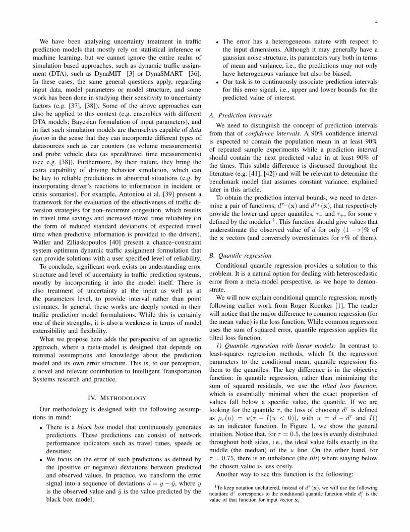
1) Quantile regression with linear models: In contrast toleast-squares regression methods, which fit the regressionparameters to the conditional mean, quantile regression fitsthem to the quantiles. The key difference is in the objectivefunction: in quantile regression, rather than minimizing thesum of squared residuals, we use the tilted loss function,which is essentially minimal when the exact proportion ofvalues fall below a specific value, the quantile. If we arelooking for the quantile τ , the loss of choosing dτ is definedas ρτ (u) = u(τ − I(u < 0)), with u = d − dτ and I()as an indicator function. In Figure 1, we show the generalintuition. Notice that, for τ = 0.5, the loss is evenly distributedthroughout both sides, i.e., the ideal value falls exactly in themiddle (the median) of the u line. On the other hand, forτ = 0.75, there is an unbalance (the tilt) where staying belowthe chosen value is less costly.

Another way to see this function is the following:

1To keep notation uncluttered, instead of dτ (x), we will use the followingnotation: dτ corresponds to the conditional quantile function while dτi is thevalue of that function for input vector xi

5

𝝉=0.5

𝝉=0.75

u

𝜌(u)

Fig. 1. Tilted loss function, ρ(u).

ρτ (di − dτ ) =

{τ(dτ − di) di >= dτ

(1− τ)(di − dτ ) di < dτ(1)

Thus, we can determine the expected loss, Eρτ (D − dτ ),of choosing dτ to be the τ quantile for random variable D,given a set of samples di, with i = 1..N :

(τ − 1)∑di<dτ

(di − dτ ) + τ∑

di>=dτ

(dτ − di) (2)

It will be rare to have a set of (training) samples, di, foreach input vector x such that we can precisely estimate itslocal quantile in this way. Instead, we can use the distributionof values throughout an entire dataset to estimate a singlefunction such that dτi = xi

Tβτ . I.e., at each input vectorxi, there will be a potentially unique quantile value, dτi , thatis a function of its components. Thus, for conditional quantileregression, we need to minimize

(τ −1)∑

(xi,di)∈Sdi<xi

Tβτ

(di−xiTβτ )+τ

∑(xi,di)∈S

di>=xiTβτ

(xiTβτ −di) (3)

with respect to the parameters βτ throughout the entire datasetS = (X,d) of size N, where for each input vector xi ∈ X,we have the corresponding observed deviation value, di ∈d. In other words, we need to estimate the values for βτsince S and τ are all given. This can be reformulated as alinear programming problem, solvable by the simplex method.We will not add further details on this procedure here, so weredirect the interested reader to Koenker’s book [1] on thesubject.

For the purpose of illustration, we created two toy modelsof the form y = ax + b + ε where ε is distributed either asN(0, x) (variance grows with x) or N(0, gp(0, 1)) (varianceis sampled from a Gaussian Processes prior). We call themnoise models 1 and 2, respectively. We assume that our (blackbox) predictor, y, corresponds to the denoised model, y =ax+ b. We then calculated the set of deviations, di = yi− yi,and applied the conditional quantile regression method justdescribed. The bounds become yτ−i = yi + d

τ−i and y

τ+i =

yi+ dτ+i , respectively for lower and upper bounds at each xi.

Plots in Figure 2 show this data together with the 5% and 95%quantile bounds given by our model. Notice that, in this case,x or y do not correspond to any real world phenomena, theyare purely chosen for demonstrative purposes.

Fig. 2. Toy model 1 (top) and model 2 (bottom). We show the underlyingpredictions (of y as a function of x) as well as the lower and upper bounds.

This procedure yields a linear model for each τ quan-tile, thus it is insufficient when the error varies non-linearlythroughout the entire dataset. A solution is to estimate anindependent model for each prediction point by applyinglocally weighted regression, essentially assigning more weightto neighboring vectors according to some distance function, for

example the squared exponential, si,j= e

(−||xi−xj||

2h2

), where h

is known as the bandwidth, and xi and xj are any two vectorsin the dataset. Thus, we rewrite equation 3 into:

(τ−1)∑

i:(xi,di)∈Sdi<xi

Tβτ

si,0(di−xiTβτ )+τ

∑i:(xi,di)∈Sdi>=xi

Tβτ

si,0(xiTβτ−di)

(4)where si,0 represents the distance between the prediction pointand vector xi from the dataset. Figure 3 illustrates the effect.The wiggly behavior is due to the preference to the local versusglobal fits. We will discuss this in the next section.

Locally weighted regression has been used with success intraffic estimation and prediction (e.g. [10], [43]), and falls inthe family of vast literature on non-parametric models such asgaussian processes [44], k-nearest neighbor regression [4] orsupport vector regression [45].

2) Quantile regression with spline models: In our context,locally linear models have three relevant problems. We need toestimate multiple individual models; such models are limitedto a linear form and as a result the overall (piece-wise linear)function is not smooth; unless the point’s neighborhood isrepresentative enough, it is more prone to overfitting than aglobal model. The two latter points are clearly visible in Figure3.

A solution to these problems proposed in [1] is to use asplines function. This function is decomposed into a sequenceof piece-wise polynomial functions that are linked together at

6

Fig. 3. Locally linear models on toy models 1 (top) and 2 (bottom).

M knot points. The splines function needs to be differentiablein all its points, including at the knots. We apply a wellknown decomposition process, the B-splines, where the splinefunction is expressed as a linear combination of Basis splineswith degree k. So now we have a new definition for dτi thatadds a splines component to the linear combination xi

Tβτdefined earlier. Formally,

dτi = xli

Tβlτ +

M+1∑m=−1

amBm(xsi ) (5)

where xli and βlτ correspond to the input features and pa-

rameters that remain in the linear part of the model, and xsi

corresponds to the input features that are applied splines. Thereis an am coefficient for each of the M + 2 cubic B-splinefunctions, Bm. Each one of these functions calculates thecontribution for xs

i of the piece-wise cubic function betweenknots m and m+1. The B-spline functions, Bm, are the subjectof extensive literature and are implemented in a wide variety ofsoftware packages. For further details, we redirect the readerto [46].

To estimate and run this model, we used the packagessplines and quantreg [47], available in R [48], together withthe objective function specified by equation 3. The mostcommon form of spline models uses a 3rd degree polynomial,the cubic splines. Unless otherwise mentioned, we will keepthis choice.

From the point of view of quantile regression, cubic splinesallow for capturing local effects while still being differentiableat every point, hence the smoothing effect and better general-ization properties.

In Figure 4, we illustrate the result with the toy model abovedescribed. In this case, we use dτi =

∑M+1m=−1 amBm(x).

We will not provide further details on quantile regressionso we redirect the interested reader to fundamental literature,

Fig. 4. Cubic splines on toy models 1 (top) and 2 (bottom).

namely Koenker’s book [1], the gentle introduction of Cadeand Noon [9], or specific contributions on local linear models[49] or application with gaussian processes [44]. We alsoadvise the use of the very well designed and complete quantileregression package, quantreg, available for R [47] for thosekeen to implement this method.

C. Prediction intervals for homoscedastic processes

As mentioned earlier, we will also use a baseline modelwhere we use a known constant (homoscedastic) variance togenerate the interval bounds for each prediction, y. First, weobtain the observed error variance from the training set, σ2,then we determine the prediction interval bounds, yτ− andyτ+ , according to

yτ± = y ± tpσ√1 + 1/n, (6)

where tp corresponds to the quantile 100((1 − p)/2)% ofStudent’s t-distribution with n-1 degrees of freedom. Suchprocedure is well know and a common practice (e.g. [50]).

D. Putting it all together

The quantile regression methods presented provide a func-tion dτ that, for any given input vector, yields the quantileat the τ level. Our method is to use 2 independent models,one for predicting the lower bound (τ−), the other for theupper bound (τ+), that will be estimated from a time series oferror deviations. For the input vector, x, we will consider theblack box predicted value, y, the time of day (peak, non peak),as well as the L auto-regression lags, i.e. L previous valuesof error. A preliminary autocorrelation analysis revealed thatL = 3 should be an acceptable value throughout the dataset,i.e. in general, up to the third lag, the signal is autocorrelated

7

by 0.5 or above. Other input features could be added trivially,such as weather status or incident information, however we donot have such information for the available datasets.

The target value is, as defined before, given by di = yi− yi,the deviation between the predicted and observed value forevery single input vector xi. Our algorithms aim to predictthe upper and lower bound values, yiτ+ and yiτ− , resp., suchthat, in 100 ∗ (τ+ − τ−)% of the times, the target value fallswithin the interval. We will choose τ+ and τ− to be 0.95 and0.05, respectively. This implies that, for the constant variancemodel, we assign tp = 1.645 (the two-sided 90% value forthe t-distribution).

E. Performance measures

While for pointwise regression the performance measuresare very well defined and accepted (e.g. root mean squarederror, correlation coefficient, relative squared error), the samecannot be said for evaluating interval regression. This happensbecause we need to consider both whether the predictedintervals did contain the target value as well as how precisetheir bounds were. In fact, if we assign extreme values tothe bounds, we trivially get an interval predictor that containsthe targets for 100% of the times. Conversely, we can alsoget very narrow intervals that repeatedly fail. A few solutionswere proposed by Khosravi et al. [8]:

• Prediction interval coverage probability (PICP),

PICP =1

n

n∑i=1

ci,

where ci = 1 if yi ∈ [yτ− , yτ+ ]

• Mean prediction interval length (MPIL),

MPIL =1

n

n∑i=1

(yτ+ − yτ−)

• Normalized MPIL, NMPIL = MPILR , with R being

defined a priori

• Coverage-length-based criterion (CLC),

CLC = NMPIL(1 + e(−η(PICP−µ))

with η and µ as two controlling parameters.

Ideally, PICP should be as close as possible to the(τ+ − τ−). In our case, this should be 0.9. For MPIL, thelowest value possible is sought. NMPIL demands a specificparameter, R, that is not clearly defined in [8], so we propose aspecific implementation, the relative mean prediction intervallength (RMPIL),

RMPIL =1

n

n∑i=1

(yτ+ − yτ−)|y − y|

i.e., we normalize the interval length by the observed error.Large intervals are in fact necessary whenever actual error

is large itself, otherwise it is not possible to cover the targetvalue.

In the CLC measure, the µ parameter has a very clearmeaning: it represents the desired PICP value. On the otherhand, the parameter η is difficult to materialize; it magnifiesthe importance of reaching the desired PICP . Furthermore,the interval length measure, NMPIL, has a potentially negli-gible role. If we have a PICP below µ, even by a very smallamount, CLC becomes unreasonably affected. For example,with µ = 0.9, η = 200 as in [8], a model with coveragevery close to the ideal such as 89% (PICP = 0.89) wouldobtain a CLC higher than NMPIL2, in fact being worse thanany other model with PICP of 0.9 or above that relaxes thebounds up to NMPIL2. In other words, unreasonably largeintervals would be preferable than a more precise model withPICP marginally below the objective.

The value of η serves to control this effect, however itschoice is arbitrary and becomes a challenge in itself. Assigninga very low value would also underestimate the importanceof PICP. After repeated empirical tests, we decided to setthe value to 100. We also propose a simpler measure, calledCLC2:

CLC2 = e(−RMPIL(PICP−µ))

This measure gives both MPIL and PICP comparableroles and removes the subjective control parameter. We willuse all defined measures just discussed in our evaluation.

V. EXPERIMENTS

A. Experimental design

Two freeway data-sets from Irvine, CA, and Tel Aviv inIsrael have been used for this research. In both cases, weekdaydata were used. The Irvine data set includes five days ofsensor data from freeway I-405. The application involvedtraining/calibration with four days of data and subsequenttesting/validation of the model framework for the fifth day (notused in the calibration). Data from 10am to 12midnight havebeen used, since this period includes the (pm) peak flow forthis direction. Speed, occupancy and flow data over 2–minuteintervals were available for calibration and validation. Occu-pancy data have been converted to density using a relationshipfrom May ([14], eq. 7.2 in p. 193).

The second data set was collected in Highway 20 (AyalonHighway), a major intra–city freeway running through thecenter of Tel Aviv in Israel. Four days of data were used forthe training of the models and a different fifth day was usedfor validation. Speed, occupancy and flow data were availableand were aggregated over 5-minute intervals. Occupancy datahave been converted to density using the same relationship asabove.

The following different cases are developed, based on thetype of approach that is used for state (where applicable) andspeed prediction:

1) Typical speed-density relationship: a commonly usedrelationship is fit to the speed and density data of thetraining data set.The following speed-density relationship model wasused as the reference model [3]:

8

u = uf

[1−

(max(0, k − kmin)

kjam

)β]α(7)

where, u denotes the space mean speed, uf the free flowspeed, k the density, kmin the minimum density, kjamthe jam density, and α and β are model parameters.This is a variant of the speed-density traffic flow theoryrelationship that is commonly used in mesoscopic trafficsimulation models. For example, this is the relationshipused in the DynaMIT model [3] and very similar tothe relationship used in the DynaSMART [36] andmezzo [51] models.The estimated relationship is then used to calculatespeed values based on the densities in the test dataset. The true densities (instead of predicted) are usedin this process, thus eliminating any prediction errorand providing an even better than expected predictionof speeds for this baseline model.

2) Speed prediction framework presented in Antoniou etal. [10]: a complete state and speed prediction frame-work has been applied using the available data. Themethodology comprises training and application steps.During the training step archived surveillance data areused to (A) identify the various traffic states throughclustering the available observations; (B) estimate thetransition processes between these regimes; and (C)estimate cluster-specific traffic models. This informationis stored into a knowledge base and supports the appli-cation of the framework. As new measurements becomeavailable, they are (D) classified into the appropriateregimes and, based on the transition processes and theshort-term evolution of the traffic state, (E) short-termpredictions of the traffic state are performed using theapplicable estimated transition processes. Furthermore,(F) the appropriate flexible traffic model is retrievedand applied to the new observations to (G) performspeed predictions. In this case, the optimal number ofstates is used, i.e. the number of states that minimizesthe Bayesian Information Criterion (BIC), based on theresults from the model-based clustering algorithm.

3) Simplified framework presented in Antoniou et al. [10]:The complete state and speed prediction framework isused, but neural networks are used for the clustering andclassification steps. This is a simpler approach that isimplemented in order to assess the incremental benefitsof the proposed framework components.

These three approaches will be our black box speed pre-diction models. Henceforth, for simplicity of reference, wewill call the first approach as spddsty; the second one will beLOESS (locally weighted scatterplot smoothing) and the lastone will be NNet.

For each dataset and each black box model, we will runour three prediction interval meta-models: with constant vari-ance (const); splines quantile regression (splines); and locallyweighted quantile regression (local). We will use the first 2/3of the dataset (ordered in time) for training and 1/3 for testing.

Fig. 5. Speed-density function performance in Ayalon.

B. Results

Table I shows the overall results obtained. Unsurprisingly,we can see that the constant variance model achieves PICPvalues close to the intended prediction interval coverage (of0.9) in all cases but it does so at the expense of the largestinterval ranges. This also indicates that the variance observedin the training set is similar to that of the test set, i.e. theyseem to be adequately balanced. Except for two models inAyalon (NNet and Loess), the quantile regression modelsobtain performance with good PICP, interval length and CLCmeasures. And we can also observe that the CLC2 measureprovides a more balanced evaluation with regards to PICP andinterval length.

TABLE IOVERALL RESULTS TABLE.

blckbx metamodel dataset model PICP MPIL RMPIL CLC CLC2Loess Irvine local 0.82 8.79 10.86 6.70E+04 2.39Loess Irvine const 0.88 9.69 12.50 1.71E+03 1.33Loess Irvine splines 0.81 8.67 10.76 8.09E+05 1.21Loess Ayalon local 0.59 4.52 5.75 2.86E+14 5.90Loess Ayalon const 0.85 8.83 11.22 3.07E+04 1.85Loess Ayalon splines 0.69 7.42 9.80 1.25E+11 6.70Spddsty Irvine local 0.74 15.04 12.83 1.47E+08 7.36Spddsty Irvine const 0.92 20.88 18.12 3.56E+02 0.638Spddsty Irvine splines 0.95 21.59 18.95 3.62E+02 0.408Spddsty Ayalon local 0.74 8.05 9.64 2.00E+08 4.75Spddsty Ayalon const 0.89 17.50 19.00 1.14E+03 1.16Spddsty Ayalon splines 0.93 12.42 12.15 1.55E+02 0.698NNet Irvine local 0.87 9.50 17.17 8.08E+02 1.51NNet Irvine const 0.88 9.56 18.07 3.57E+03 1.71NNet Irvine splines 0.88 10.05 19.33 4.08E+03 1.56NNet Ayalon local 0.66 4.44 15.43 6.71E+11 5.61NNet Ayalon const 0.86 9.53 42.22 1.08E+05 39.4NNet Ayalon splines 0.69 6.46 23.75 7.34E+11 146

Before getting into further details, let us take a quick lookat a few of the error signals, di. Figures 5, 6, 7 and 8 show afew examples. Due to space constraints, we focus on the morechallenging case of Ayalon, adding an example from Irvine.

There is a striking difference in variance between thespeed/density function and the other two models. And itcould be argued that this variance changes in time (x axis)

9

Fig. 6. Neural network performance in Ayalon.

Fig. 7. LOESS performance in Ayalon.

Fig. 8. Speed-density function performance in Irvine.

Fig. 9. Prediction intervals for Ayalon speed density model based on splines.

in all cases, particularly for the speed/density function. Forthe Irvine case, we can say that the same behavior applies,although less sharply. Recalling Table I, the obvious interpre-tation is that quantile regression is a good option for cases withhigh, heteroscedastic, variance but, under lower and less variederror, the traditional confidence/prediction intervals approachmay be ideal if we value coverage (PICP ) more than intervallength (RMPIL).

To better illustrate the actual performance of the algorithms,we plot the prediction intervals through time between thesplines quantile regression and constant variance models, fortwo black boxes: speed density (Figures 9 and 10) and LOESS(Figures 11 and 12). Obviously, constant variance modelalways generates the same interval length, so its coveragedepends essentially on the bias of the model. The speeddensity function model seems more biased but together withthe splines model it is clearly capable obtaining the bestperformance. If we take a look at CLC2, this same conclusionwould apply to the Irvine case, although it is arguable that thesplines quantile regression obtained unnecessarily high PICPat the expense of intervals that are much larger than necessary.Figure 13 illustrates this point.

VI. DISCUSSION

In this article, we demonstrate a methodology that is ca-pable of obtaining prediction interval bounds for a black boxpredictor that depends on very few weak assumptions. Theseare: the error quantile bounds of the target variable can bedefined as a function of some available input vector x; thisfunction has either a linear or polynomial form (potentiallycomposed into a global splines model); and the training andtest sets should be independently and identically distributed(iid). There are no other constraints with respect to the errorform or the properties of the black box model.

Of course, this versatility does not come without a cost:being disconnected from the source itself (the black boxmodel) implies that we are treating the effects, not the cause.If the traffic prediction engine has very poor performance, our

10

Fig. 10. Prediction intervals for Ayalon speed density model based onconstant variance.

Fig. 11. Prediction intervals for Ayalon LOESS model based on splines.

Fig. 12. Prediction intervals for Ayalon LOESS model based on constantvariance.

algorithm won’t do more than emphasizing it more clearly, by

Fig. 13. Prediction intervals for Irvine spddsty model based on splines.

Fig. 14. Slack box plots for Ayalon spddsty model.

providing very large bounds.We could see that, from the experiments, it is not trivial

to evaluate the quality of our three models independently ofthe quality of the underlying predictions. For example, if theobserved speed value is 50km/h and the predictor gives 120km/h, then the ideal meta-model should only allow enoughslack to cover these two values2. In this case, the smallestslack would be 120−50 = 80 and any higher value would beerring on the conservative side, while a lower value wouldbe failing to cover the observed value. The RMPIL wasdesigned to capture this effect, but we can better see howthe several algorithms behave in terms of slack amounts witha visualization. Figures 14 and 15 present the box plots for thespeed density function and LOESS for Ayalon, respectively.We show the (extra) slack performance for each of the threemeta-models. On the x axis, we show the observed speed.

In practice, a box plot for a good model should be centeredslightly above 0, preferably enough not to go below that

2We are assuming that the predicted value should be contained in theinterval. In our experiments, this was generally the case but the models couldlearn otherwise.

11

Fig. 15. Slack box plots for Ayalon LOESS model.

value. I.e., it would provide just enough slack above the idealinterval length, to err on the conservative side. Except for afew exceptions, we can clearly see that the constant variancemodel chooses the largest intervals. The splines model seemsto be better than the local one in the sense that the latterobtains more negative slacks. This is coherent with what wesee in Figures 3 and 4 of our toy model and with the relateddiscussion on over fitting and smoothness.

Let us now summarize a few other observations from theexperiments:

• The quantile models rarely underestimate the upperbound but sometimes overestimate the lower bound.This can be concerning in the case of speeds since itcorresponds to an optimistic perspective. For example,DynaMIT2.0 may fail to anticipate congestions properly;

• As a consequence of the above, the PICP in some ofthe quantile models is very low, particularly for AyalonNNet and Loess. The constant variance model definitelyworks better in those cases but we note that it is at theexpense of large intervals (in the NNet, the RMPIL is42.22);

• After testing with changing the splines degree to othervalues {1,2,4,5}, the performance degrades;

• After testing different bandwidths, h, for the locallyweighted quantile regression {5, 10, 50, 100, 200}, thevalue that provides best results, used throughout theexperiments. is 100. This is the best balance betweenoverfitting (small values) and noise (high values) for thisspecific dataset, but we cannot speculate further about itsmeaning.

• In terms of computational performance, these algorithmsspent negligible time in training and prediction on ourdataset. However, the case study deals with a singlesensor for each case study and a dense network coveragemight lead to non-negligible run times. It is expectablethat the locally weighted regression model degrades fastwith dataset size because it effectively estimates andpredicts a new model for each query. The splines modelwill be slower to estimate but this can be done on an off-

line basis. The constant variance model obviously posesminimal constraints to dataset size and can be estimatedon an off-line basis.

An important issue may arise when using conditional quan-tile regression: the problem of crossed quantiles, when, fora given xi, the upper quantile is below the lower quantile.We were minimally affected by this phenomenon so it wasneglected in the work presented. However, it deserves a morecautious treatment in practice, particularly in light of availableliterature on the subject (e.g. [52], [53]).

Another concern relates to the sensitivity of the model totraffic state dynamics. We want a model that, under stressconditions, is able to keep the expected reliability. While it isnot easy to replicate or identify such conditions in our dataset,we can get some insights by comparing the performance forpeak/off-peak periods. Starting with the splines model, wesee a somewhat surprising result: during peak periods, itsPICP actually increases in all cases (e.g. it improves from0.87 to 0.91 in Irvine NNet). This obviously happens at theexpense of larger prediction intervals. Our intuition is that,given similar circumstances in the training set (higher localvariance), the quantiles will tend to err on the safe side. For thehomoscedastic model, the opposite happens (e.g. it degradesfrom 0.89 to 0.55 in Irvine NNet), which is not surprisinggiven the total lack of flexibility of this model. Finally, thelocally weighted quantile regression model presents mixedresults (e.g. it improves from 0.73 to 0.93 in Irvine NNet,while it degrades from 0.88 to 0.81 in Irvine Loess). We shouldhowever be cautious in this analysis despite these results beingencouraging. Traffic state dynamics will probably be morechallenging under exceptional circumstances (e.g. incidents,special events, harsh weather) than the duality of peak/off-peak. Further work will need to be done at this respect.

Finally, these experiments intended to test our methodologywithout pretending an immediate real-world application withthese black box models. Although relevant for this trial, thedataset is somewhat poor in contextual detail that shouldactually improve the prediction interval capabilities. For ex-ample, having information on incidents, weather or specialevents would certainly lead to a more meaningful real-worldapplication.

VII. CONCLUSIONS AND FUTURE WORK

We introduced a meta-model methodology that is capableof estimating, in real-time, the prediction intervals for a trafficprediction system by analyzing its error history. It does soby applying conditional quantile regression to the time seriessignal of the observed error and also considering the predictedvalue itself. The lower and upper bounds become simply thelower and upper quantiles, as per choice of the modeler. Weimplemented this concept and tested it with two case-studiesin Israel and California, USA. In each case-study, the originalprediction task consisted of predicting speeds from senseddensities.

We compared our prediction interval methodology witha constant variance baseline and the experiments show thatquantile regression approaches are capable of determining

12

smaller prediction intervals and comparable accuracy (or pre-diction interval coverage probability, PICP ) in most cases.More importantly, under high variance and heteroscedascity,our approach is more adequate than using traditional confi-dence intervals. This is particularly relevant when the errorstructure is not known.

We specifically applied this concept to speed prediction butit can be tested with any other regression task with very littleeffort. For example, if we want to add interval predictioncapabilities to an existing bus arrival prediction algorithm, weonly need access to the feed of predictions and observationsas well as any other variable that is believed to correlate tothe prediction error (e.g. traffic conditions, weather status).The model implementation and experimental methodologiesare essentially the same as in this paper.

Future research includes an investigation into the role ofdifferent network geometry and other characteristics into theperformance of the presented approach, as well as the impactof different prediction intervals. In this work, a preliminaryassessment of the robustness of the approach was achievedby looking at data from different networks (i.e. Israel vs.California), and different prediction intervals (i.e. 2 vs 5 min).

We also introduced two new performance measures that aimto better evaluate prediction interval models, both extendingthe previous work of Khosravi et al. [8] aiming for a betterbalance between PICP and interval length. We add the notionof slack as the ideal interval length corresponding to thedifference between observed and predicted.

The next step consists of the extension of this work withthe gaussian processes algorithm, from a Bayesian approachperspective, building on the work from Boukouvalas et al.[44] and Lazaro-Gredilla et al. [7]. We expect a performanceat least comparable to the splines model, while becominga very good solution for online learning. Any real-worldimplementation of a prediction intervals meta-model needs toaccompany performance evolution of its associated predictionmodel (online learning).

This project is integrated in the DynaMIT2.0 framework,and participates both as an input data quality estimator aswell as a service for the end user, providing upper and lowerbounds for predictions of traffic information such as traveltimes, speeds or volumes.

ACKNOWLEDGMENTS

The authors would like to thank Prof. Wilfred Recker fromUniversity of California, Irvine, and Dr. Tomer Toledo fromTechnion Institute of Technology, Israel, for providing thedata used in this research. The authors would like to thankthe anonymous reviewers for their insightful comments thatstrongly contributed to the improvement of this article.

This research was supported by the National ResearchFoundation Singapore through the Singapore MIT Alliance forResearch and Technology’s FM IRG research programme.

REFERENCES

[1] R. Koenker, Quantile Regression. Cambridge University Press, 2005.

[2] M. Ben-Akiva, M. Bierlaire, D. Burton, H. Koutsopoulos, and R. Misha-lani, “Network state estimation and prediction for real-time trafficmanagement,” Networks and Spatial Economics, vol. 1, no. 3-4, pp.293–318, 2001.

[3] M. Ben-Akiva, H. N. Koutsopoulos, C. Antoniou, and R. Balakrishna,“Traffic simulation with dynamit,” in Fundamentals of Traffic Simula-tion, J. Barcelo, Ed. New York, NY, USA: Springer, 2010, pp. 363–398.

[4] P. M. Robinson, “Asymptotically efficient estimation in the presence ofheteroskedasticity of unknown form,” Econometrica, vol. 55, no. 4, pp.875–891, 1987.

[5] S. Chib and E. Greenberg, “On conditional variance estimation innonparametric regression,” Statistics and Computing, vol. 23, pp. 261–270, 2013.

[6] H. White, “A heteroskedasticity-consistent covariance matrix estimatorand a direct test for heteroskedasticity,” Econometrica, vol. 48, pp. 817–838, 1980.

[7] M. Lazaro-gredilla and M. K. Titsias, “Variational heteroscedastic gaus-sian process regression,” in In 28th International Conference on MachineLearning (ICML-11). ACM, 2011, pp. 841–848.

[8] A. Khosravi, E. Mazloumi, S. Nahavandi, D. Creighton, and J. W. C.Van Lint, “Prediction intervals to account for uncertainties in travel timeprediction,” Intelligent Transportation Systems, IEEE Transactions on,vol. 12, no. 2, pp. 537–547, 2011.

[9] B. S. Cade and B. R. Noon, “A gentle introduction to quantile regressionfor ecologists,” Frontiers in Ecology and the Environment, vol. 1, no. 8,pp. 412–420, 2003.

[10] C. Antoniou, H. N. Koutsopoulos, and G. Yannis, “Dynamicdata-driven local traffic state estimation and prediction,”Transportation Research Part C: Emerging Technologies,vol. 34, pp. 89 – 107, 2013. [Online]. Available:http://www.sciencedirect.com/science/article/pii/S0968090X13001137

[11] S. Shalev-Shwartz, “Online Learning: Theory, Algorithms, and Appli-cations,” Ph.D. dissertation, The Hebrew University of Jerusalem, Jul.2007.

[12] M. Neumann, K. Kersting, Z. Xu, and D. Schulz, “Stacked gaussianprocess learning,” in Data Mining, 2009. ICDM ’09. Ninth IEEEInternational Conference on, 2009, pp. 387–396.

[13] C. Antoniou, M. Ben-Akiva, and H. N. Koutsopoulos, “Nonlinearkalman filtering algorithms for on-line calibration of dynamic trafficassignment models,” Intelligent Transportation Systems, IEEE Transac-tions on, vol. 8, no. 4, pp. 661–670, 2007.

[14] A. May, Traffic Flow Fundamentals. New Jersey: Prentice Hall, 1990.[15] M. A. Abdel-Aty, R. Kitamura, and P. P. Jovanis, “Using stated

preference data for studying the effect of advanced traffic informationon drivers’ route choice,” Transportation Research Part C: EmergingTechnologies, vol. 5, no. 1, pp. 39–50, 1997.

[16] H. S. Mahmassani and Y.-H. Liu, “Dynamics of commuting decisionbehaviour under advanced traveller information systems,” TransportationResearch Part C: Emerging Technologies, vol. 7, no. 2, pp. 91–107,1999.

[17] T. Toledo and R. Beinhaker, “Evaluation of the potential benefits ofadvanced traveler information systems,” Journal of Intelligent Trans-portation Systems, vol. 10, no. 4, pp. 173–183, 2006.

[18] D. Ettema and H. Timmermans, “Costs of travel time uncertainty andbenefits of travel time information: conceptual model and numericalexamples,” Transportation Research Part C: Emerging Technologies,vol. 14, no. 5, pp. 335–350, 2006.

[19] G. De Jong, A. Daly, M. Pieters, S. Miller, R. Plasmeijer, and F. Hofman,“Uncertainty in traffic forecasts: literature review and new results for thenetherlands,” Transportation, vol. 34, no. 4, pp. 375–395, 2007.

[20] T. Park and S. Lee, “A bayesian approach for estimating link traveltime on urban arterial road network,” in Computational Science and ItsApplications ICCSA 2004, ser. Lecture Notes in Computer Science,A. Lagan, M. Gavrilova, V. Kumar, Y. Mun, C. Tan, and O. Gervasi,Eds. Springer Berlin Heidelberg, 2004, vol. 3043, pp. 1017–1025.

[21] S. Sun, C. Zhang, and G. Yu, “A bayesian network approach to trafficflow forecasting,” Intelligent Transportation Systems, IEEE Transactionson, vol. 7, no. 1, pp. 124–132, 2006.

[22] S. Sun and C. Zhang, “The selective random subspace predictor fortraffic flow forecasting,” Intelligent Transportation Systems, IEEE Trans-actions on, vol. 8, no. 2, pp. 367–373, 2007.

[23] Y. Gao, S. Sun, and D. Shi, “Network-scale traffic modeling andforecasting with graphical lasso,” in Advances in Neural Networks ISNN2011, ser. Lecture Notes in Computer Science, D. Liu, H. Zhang,M. Polycarpou, C. Alippi, and H. He, Eds. Springer Berlin Heidelberg,2011, vol. 6676, pp. 151–158.

13

[24] N. Djuric, V. Radosavljevic, V. Coric, and S. Vucetic, “Travel speedforecasting by means of continuous conditional random fields,” Trans-portation Research Record: Journal of the Transportation ResearchBoard, no. 2263, pp. 131–139, 2011.

[25] J. Van Lint, “Reliable real-time framework for short-term freeway traveltime prediction,” Journal of transportation engineering, vol. 132, no. 12,pp. 921–932, 2006.

[26] C. van Hinsbergen, J. van Lint, and H. van Zuylen,“Bayesian committee of neural networks to predict traveltimes with confidence intervals,” Transportation Research PartC: Emerging Technologies, vol. 17, no. 5, pp. 498 – 509,2009, ¡ce:title¿Artificial Intelligence in Transportation Analysis:Approaches, Methods, and Applications¡/ce:title¿. [Online]. Available:http://www.sciencedirect.com/science/article/pii/S0968090X09000357

[27] S. Sun and X. Xu, “Variational inference for infinite mixtures of gaussianprocesses with applications to traffic flow prediction,” Intelligent Trans-portation Systems, IEEE Transactions on, vol. 12, no. 2, pp. 466–475,2011.

[28] Y. Xie, K. Zhao, Y. Sun, and D. Chen, “Gaussian processes forshort-term traffic volume forecasting,” Transportation Research Record:Journal of the Transportation Research Board, no. 2165, pp. 69–78,2010.

[29] X. Fei, C.-C. Lu, and K. Liu, “A bayesian dynamic linear modelapproach for real-time short-term freeway travel time prediction,” Trans-portation Research Part C: Emerging Technologies, vol. 19, no. 6, pp.1306–1318, 2011.

[30] B. Ghosh, B. Basu, and M. OMahony, “Bayesian time-series model forshort-term traffic flow forecasting,” Journal of transportation engineer-ing, vol. 133, no. 3, pp. 180–189, 2007.

[31] E. Mazloumi, G. Rose, G. Currie, and S. Moridpour, “Predictionintervals to account for uncertainties in neural network predictions:Methodology and application in bus travel time prediction,” EngineeringApplications of Artificial Intelligence, vol. 24, no. 3, pp. 534–542, 2011.

[32] E. Mazloumi, G. Rose, G. Currie, and M. Sarvi, “An integrated frame-work to predict bus travel time and its variability using traffic flow data,”Journal of Intelligent Transportation Systems, vol. 15, no. 2, pp. 75–90,2011.

[33] A. Khosravi, E. Mazloumi, S. Nahavandi, D. Creighton, and J. Van Lint,“Prediction intervals to account for uncertainties in travel time predic-tion,” Intelligent Transportation Systems, IEEE Transactions on, vol. 12,no. 2, pp. 537–547, 2011.

[34] ——, “A genetic algorithm-based method for improving quality of traveltime prediction intervals,” Transportation Research Part C: EmergingTechnologies, vol. 19, no. 6, pp. 1364–1376, 2011.

[35] A. Khosravi, S. Nahavandi, D. Creighton, and A. F. Atiya, “Compre-hensive review of neural network-based prediction intervals and newadvances,” Neural Networks, IEEE Transactions on, vol. 22, no. 9, pp.1341–1356, 2011.

[36] H. S. Mahmassani, “Dynamic network traffic assignment and simulationmethodology for advanced system management applications,” Networksand Spatial Economics, vol. 1, no. 3-4, pp. 267–292, 2001.

[37] B. Park, J. Lee, D. Pampati, and B. Smith, “Online implementation ofdynamit: A prototype traffic estimation and prediction program,” KSCEJournal of Civil Engineering, vol. 12, no. 2, pp. 129–140, 2008.

[38] C. Antoniou, On-line calibration for Dynamic Traffic Assignmentmodels- Theory, methods and application. Saarbrucken, Germany,Germany: VDM Verlag, 2007.

[39] C. Antoniou, H. N. Koutsopoulos, M. Ben-Akiva, and A. S. Chauhan,“Evaluation of diversion strategies using dynamic traffic assignment,”Transportation Planning and Technology, vol. 34, no. 3, pp. 199–216,2011.

[40] S. Travis Waller and A. K. Ziliaskopoulos, “A chance-constrained basedstochastic dynamic traffic assignment model: Analysis, formulationand solution algorithms,” Transportation Research Part C: EmergingTechnologies, vol. 14, no. 6, pp. 418–427, 2006.

[41] T. Heskes, “Practical confidence and prediction intervals,” in Advancesin Neural Information Processing Systems 9. MIT press, 1997, pp.176–182.

[42] D. R. Cox, “Prediction intervals and empirical bayes confidence inter-vals,” in Perspectives in Probability and Statistics. Academic Press,1975, pp. 45–55.

[43] T. Toledo, H. N. Koutsopoulos, and K. Ahmed, “Estimation of vehicletrajectories with locally weighted regression,” Transportation ResearchRecord: Journal of the Transportation Research Board, no. 1999, pp.161–169, 2007.

[44] A. Boukouvalas, R. Barillec, and D. Cornford, “Gaussian process quan-tile regression using expectation propagation,” in In 29th International

Conference on Machine Learning (ICML-12). Edinburgh, Scotland,UK, 2012, 2012.

[45] K. De Brabanter, J. De Brabanter, J. A. K. Suykens, and B. De Moor,“Approximate confidence and prediction intervals for least squaressupport vector regression,” Neural Networks, IEEE Transactions on,vol. 22, no. 1, pp. 110–120, 2011.

[46] T. Hastie and R. Tibshirani, “Generalized additive models,” Statisticalscience, pp. 297–310, 1986.

[47] R. Koenker, quantreg: Quantile Regression, 2013, r package version4.98. [Online]. Available: http://CRAN.R-project.org/package=quantreg

[48] R Core Team, R: A Language and Environment for StatisticalComputing, R Foundation for Statistical Computing, Vienna, Austria,2013. [Online]. Available: http://www.R-project.org/

[49] K. Yu and M. C. Jones, “Local linear quantile regression,” Journal of theAmerican Statistical Association, vol. 93, no. 441, pp. 228–237, 1998.

[50] S. Geisser, Predictive Inference: An Introduction. CRC Press, 1993.[51] W. Burghout, H. N. Koutsopoulos, and I. Andreasson, “Hybrid

mesoscopic–microscopic traffic simulation,” Transportation ResearchRecord: Journal of the Transportation Research Board, no. 1934, pp.218–225, 2005.

[52] H. Dette and S. Volgushev, “Non-crossing non-parametric estimatesof quantile curves,” Journal of the Royal Statistical Society: Series B(Statistical Methodology), vol. 70, no. 3, pp. 609–627, 2008.

[53] V. Chernozhukov, I. Fernandez-Val, and A. Galichon, “Quantile andprobability curves without crossing,” Econometrica, vol. 78, no. 3, pp.1093–1125, 2010.

Francisco C. Pereira is Senior Research Scientist in Singapore-MIT Alliancefor Research and Technology, Future Urban Mobility Integrated ResearchGroup (FM/IRG), where he is working in real-time traffic prediction, behaviormodeling, and advanced data collection technologies. In these projects, heapplies his research on data mining and pattern recognition applied to unstruc-tured contextual sources (e.g. web, news feeds, etc.) to extract informationrelevant to mobility. He is also a Professor in the University of Coimbra,Portugal from where he has a PhD degree, and a co-founder of the AmbientIntelligence Lab of that University. He led the development of several projectsthat apply these context mining principles, some with collaboration otherMIT groups such as the Senseable City Lab, where he worked earlier asa postdoctoral fellow.

Constantinos Antoniou is Assistant Professor in the National TechnicalUniversity of Athens (NTUA), Greece. He holds a Diploma in Civil En-gineering from NTUA (1995), a MS in Transportation (1997) and a PhDin Transportation Systems (2004), both from MIT. His research focuses onmodelling and simulation of transportation systems, Intelligent TransportSystems (ITS), calibration and optimization applications, road safety andsustainable transport systems. He has authored more than 150 scientificpublications, including more than 45 papers in international, peer-reviewedjournals. He is a member of several professional and scientific organizations,editorial boards (incl. Transportation Research – Part C and the Interna-tional Journal of Transportation) and committees (incl. TRB committeesAND20 – User Information Systems and AHB45 – Traffic Flow Theory).For more information please see http://users.ntua.gr/antoniou; contact him atantoniou@central.ntua.gr.

Moshe Ben-Akiva is the Edmund K. Turner Professor of Civil and Environ-mental Engineering at the Massachusetts Institute of Technology (MIT), andDirector of the MIT Intelligent Transportation Systems (ITS) Lab. He holdsa Ph.D. degree in Transportation Systems from MIT and 4 honorary degreesand coauthored the textbook Discrete Choice Analysis.