EUROPEAN ORGANIZATION FOR NUCLEAR RESEARCH

CERN-EP-2000-100July 20th 2000

A Measurement of the Rate of CharmProduction in W Decays

The OPAL Collaboration

Abstract

Using data recorded at centre–of–mass energies around 183 GeV and 189 GeV with the OPAL detectorat LEP, the fundamental coupling of the charm quark to the W boson has been studied. The ratioRW

c ≡ Γ (W → cX)/Γ (W → hadrons) has been measured from jet properties, lifetime information,and leptons produced in charm decays. A value compatible with the Standard Model expectation of0.5 is obtained: RW

c = 0.481±0.042 (stat.)±0.032 (syst.). By combining this result with measurementsof the W boson total width and hadronic branching ratio, the magnitude of the CKM matrix element|Vcs| is determined to be |Vcs| = 0.969 ± 0.058.

(Submitted to Physics Letters B)

The OPAL Collaboration

G. Abbiendi2, K.Ackerstaff8, C.Ainsley5, P.F. Akesson3, G.Alexander22, J.Allison16,K.J.Anderson9, S.Arcelli17, S.Asai23, S.F.Ashby1, D. Axen27, G. Azuelos18,a, I. Bailey26, A.H. Ball8,

E. Barberio8, R.J. Barlow16, S. Baumann3, T.Behnke25, K.W. Bell20, G.Bella22, A. Bellerive9,G. Benelli2, S. Bentvelsen8, S. Bethke32, O.Biebel32, I.J. Bloodworth1, O.Boeriu10, P.Bock11,

J. Bohme14,h, D.Bonacorsi2, M. Boutemeur31, S. Braibant8, P. Bright-Thomas1, L. Brigliadori2,R.M. Brown20, H.J. Burckhart8, J. Cammin3, P.Capiluppi2, R.K. Carnegie6, A.A. Carter13,

J.R.Carter5, C.Y. Chang17, D.G. Charlton1,b, P.E.L. Clarke15, E.Clay15, I. Cohen22, O.C.Cooke8,J. Couchman15, C.Couyoumtzelis13, R.L. Coxe9, A.Csilling15,j , M. Cuffiani2, S.Dado21,

G.M. Dallavalle2 , S.Dallison16, A. de Roeck8, E. de Wolf8, P. Dervan15, K. Desch25, B. Dienes30,h,M.S.Dixit7, M.Donkers6, J.Dubbert31, E. Duchovni24, G. Duckeck31, I.P. Duerdoth16,

P.G. Estabrooks6, E. Etzion22, F. Fabbri2, M. Fanti2, L. Feld10, P. Ferrari12, F. Fiedler8, I. Fleck10,M.Ford5, A. Frey8, A. Furtjes8, D.I. Futyan16, P. Gagnon12, J.W. Gary4, G. Gaycken25,

C.Geich-Gimbel3, G. Giacomelli2, P.Giacomelli8 , D. Glenzinski9, J.Goldberg21, C.Grandi2,K.Graham26, E.Gross24, J.Grunhaus22, M. Gruwe25, P.O. Gunther3, C.Hajdu29, G.G. Hanson12,M. Hansroul8, M. Hapke13, K.Harder25, A. Harel21, M.Harin-Dirac4, A. Hauke3, M.Hauschild8,

C.M.Hawkes1, R.Hawkings8, R.J.Hemingway6, C.Hensel25, G.Herten10, R.D. Heuer25, J.C.Hill5,A. Hocker9, K.Hoffman8, R.J.Homer1, A.K. Honma8, D. Horvath29,c, K.R.Hossain28, R. Howard27,

P. Huntemeyer25, P. Igo-Kemenes11, K. Ishii23, F.R. Jacob20, A. Jawahery17, H. Jeremie18,C.R. Jones5, P. Jovanovic1, T.R. Junk6, N. Kanaya23, J.Kanzaki23, G.Karapetian18, D. Karlen6,

V.Kartvelishvili16, K.Kawagoe23, T.Kawamoto23, R.K.Keeler26, R.G. Kellogg17, B.W. Kennedy20,D.H. Kim19, K.Klein11, A.Klier24, S.Kluth32, T. Kobayashi23, M. Kobel3, T.P. Kokott3,

S.Komamiya23, R.V. Kowalewski26, T.Kress4, P. Krieger6, J. von Krogh11, T.Kuhl3, M. Kupper24,P. Kyberd13, G.D. Lafferty16, H. Landsman21, D. Lanske14, I. Lawson26, J.G. Layter4, A. Leins31,

D. Lellouch24, J. Letts12, L. Levinson24, R. Liebisch11, J. Lillich10, B. List8, C. Littlewood5,A.W. Lloyd1, S.L. Lloyd13, F.K. Loebinger16, G.D. Long26, M.J. Losty7, J. Lu27, J. Ludwig10,

A. Macchiolo18, A.Macpherson28,m, W. Mader3, S.Marcellini2, T.E.Marchant16, A.J.Martin13,J.P. Martin18, G. Martinez17, T.Mashimo23, P.Mattig24, W.J. McDonald28, J.McKenna27,

T.J.McMahon1, R.A. McPherson26, F. Meijers8, P. Mendez-Lorenzo31, W.Menges25, F.S.Merritt9,H. Mes7, A. Michelini2, S.Mihara23, G. Mikenberg24, D.J. Miller15, W.Mohr10, A.Montanari2,T.Mori23, K.Nagai8, I. Nakamura23, H.A. Neal12,f , R. Nisius8, S.W.O’Neale1, F.G. Oakham7,

F.Odorici2, H.O.Ogren12, A. Oh8, A.Okpara11, M.J. Oreglia9, S.Orito23, G. Pasztor8,j , J.R.Pater16,G.N. Patrick20, J. Patt10, P. Pfeifenschneider14,i, J.E. Pilcher9, J. Pinfold28, D.E. Plane8, B. Poli2,

J. Polok8, O.Pooth8, M. Przybycien8,d, A. Quadt8, C. Rembser8, P. Renkel24, H. Rick4, N. Rodning28,J.M. Roney26, S. Rosati3, K.Roscoe16, A.M. Rossi2, Y. Rozen21, K.Runge10, O.Runolfsson8,D.R. Rust12, K. Sachs6, T. Saeki23, O. Sahr31, E.K.G. Sarkisyan22, C. Sbarra26, A.D. Schaile31,O. Schaile31, P. Scharff-Hansen8, M. Schroder8, M. Schumacher25, C. Schwick8, W.G. Scott20,R. Seuster14,h, T.G. Shears8,k, B.C. Shen4, C.H. Shepherd-Themistocleous5, P. Sherwood15,

G.P. Siroli2, A. Skuja17, A.M. Smith8, G.A. Snow17, R. Sobie26, S. Soldner-Rembold10,e, S. Spagnolo20,M. Sproston20, A. Stahl3, K. Stephens16, K. Stoll10, D. Strom19, R. Strohmer31, L. Stumpf26,

B. Surrow8, S.D.Talbot1, S. Tarem21, R.J. Taylor15, R. Teuscher9, M. Thiergen10, J. Thomas15,M.A. Thomson8, E. Torrence9, S. Towers6, D. Toya23, T.Trefzger31, I. Trigger8, Z.Trocsanyi30,g,

E. Tsur22, M.F. Turner-Watson1, I. Ueda23, B. Vachon26, P. Vannerem10, M. Verzocchi8, H. Voss8,J. Vossebeld8, D. Waller6, C.P.Ward5, D.R. Ward5, P.M. Watkins1, A.T.Watson1, N.K.Watson1,P.S.Wells8, T.Wengler8, N.Wermes3, D. Wetterling11 J.S.White6, G.W. Wilson16, J.A.Wilson1,

T.R.Wyatt16, S.Yamashita23, V. Zacek18, D. Zer-Zion8,l

1

1School of Physics and Astronomy, University of Birmingham, Birmingham B15 2TT, UK2Dipartimento di Fisica dell’ Universita di Bologna and INFN, I-40126 Bologna, Italy3Physikalisches Institut, Universitat Bonn, D-53115 Bonn, Germany4Department of Physics, University of California, Riverside CA 92521, USA5Cavendish Laboratory, Cambridge CB3 0HE, UK6Ottawa-Carleton Institute for Physics, Department of Physics, Carleton University, Ottawa, OntarioK1S 5B6, Canada7Centre for Research in Particle Physics, Carleton University, Ottawa, Ontario K1S 5B6, Canada8CERN, European Organisation for Nuclear Research, CH-1211 Geneva 23, Switzerland9Enrico Fermi Institute and Department of Physics, University of Chicago, Chicago IL 60637, USA10Fakultat fur Physik, Albert Ludwigs Universitat, D-79104 Freiburg, Germany11Physikalisches Institut, Universitat Heidelberg, D-69120 Heidelberg, Germany12Indiana University, Department of Physics, Swain Hall West 117, Bloomington IN 47405, USA13Queen Mary and Westfield College, University of London, London E1 4NS, UK14Technische Hochschule Aachen, III Physikalisches Institut, Sommerfeldstrasse 26-28, D-52056 Aachen,Germany15University College London, London WC1E 6BT, UK16Department of Physics, Schuster Laboratory, The University, Manchester M13 9PL, UK17Department of Physics, University of Maryland, College Park, MD 20742, USA18Laboratoire de Physique Nucleaire, Universite de Montreal, Montreal, Quebec H3C 3J7, Canada19University of Oregon, Department of Physics, Eugene OR 97403, USA20CLRC Rutherford Appleton Laboratory, Chilton, Didcot, Oxfordshire OX11 0QX, UK21Department of Physics, Technion-Israel Institute of Technology, Haifa 32000, Israel22Department of Physics and Astronomy, Tel Aviv University, Tel Aviv 69978, Israel23International Centre for Elementary Particle Physics and Department of Physics, University ofTokyo, Tokyo 113-0033, and Kobe University, Kobe 657-8501, Japan24Particle Physics Department, Weizmann Institute of Science, Rehovot 76100, Israel25Universitat Hamburg/DESY, II Institut fur Experimental Physik, Notkestrasse 85, D-22607 Ham-burg, Germany26University of Victoria, Department of Physics, P O Box 3055, Victoria BC V8W 3P6, Canada27University of British Columbia, Department of Physics, Vancouver BC V6T 1Z1, Canada28University of Alberta, Department of Physics, Edmonton AB T6G 2J1, Canada29Research Institute for Particle and Nuclear Physics, H-1525 Budapest, P O Box 49, Hungary30Institute of Nuclear Research, H-4001 Debrecen, P O Box 51, Hungary31Ludwigs-Maximilians-Universitat Munchen, Sektion Physik, Am Coulombwall 1, D-85748 Garching,Germany32Max-Planck-Institute fur Physik, Fohring Ring 6, 80805 Munchen, Germanya and at TRIUMF, Vancouver, Canada V6T 2A3b and Royal Society University Research Fellowc and Institute of Nuclear Research, Debrecen, Hungaryd and University of Mining and Metallurgy, Cracowe and Heisenberg Fellowf now at Yale University, Dept of Physics, New Haven, USAg and Department of Experimental Physics, Lajos Kossuth University, Debrecen, Hungaryh and MPI Muncheni now at MPI fur Physik, 80805 Munchenj and Research Institute for Particle and Nuclear Physics, Budapest, Hungaryk now at University of Liverpool, Dept of Physics, Liverpool L69 3BX, UKl and University of California, Riverside, High Energy Physics Group, CA 92521, USAm and CERN, EP Div, 1211 Geneva 23.

2

1 Introduction

Since 1997 the LEP e+e− collider has been operated at energies above the threshold for W-pairproduction. This offers a unique opportunity to study the hadronic decays of W bosons in a cleanenvironment and to investigate the coupling strength of W bosons to different quark flavours. Thefraction of W bosons decaying hadronically to different quark flavours is proportional to the sum ofthe squared magnitudes of the corresponding elements of the Cabibbo–Kobayashi–Maskawa (CKM)matrix [1]. A measurement of the production rates of different flavours therefore gives access to theindividual CKM matrix elements.

In e+e− → W+W− events, the only heavy quark commonly produced is the charm quark. Theproduction of bottom quarks is in fact highly suppressed due to the small magnitude of |Vub| and |Vcb|and the large mass of the top quark, the weak partner of the bottom quark. This allows for a directmeasurement of the production fraction of charm in W decays without a separation of charm andbottom quarks. The magnitude of the CKM matrix element Vcs can then be derived from the charmproduction rate, using the knowledge of the other CKM matrix elements. So far direct measurementsof |Vcs| have limited precision compared to the other CKM matrix elements important in W decays,i.e. |Vud|, |Vus|, and |Vcd|. The most recent evaluation of the magnitude of Vcs from exclusive charmsemielectronic decays yields |Vcs| = 1.04 ± 0.16 [2].

In the analysis presented here, a value of the partial decay width RWc ≡ Γ (W → cX)/Γ (W →

hadrons) is extracted from the properties of final state particles in W decays. Charm hadron iden-tification is based upon jet properties, lifetime information, and semileptonic decay products inW+W− → qqqq and W+W− → qq`ν` events. The measured value of RW

c is then used to deter-mine |Vcs|.

2 Data and Monte Carlo Samples

The data used for this analysis were recorded at LEP by the OPAL detector [3] at centre–of–massenergies around 183 GeV in 1997 and 189 GeV in 1998. OPAL1 is a multipurpose high energy physicsdetector incorporating excellent charged and neutral particle detection and measurement capabilities.The integrated luminosities used for the analysis amount to 56.5 pb−1 (180.2 pb−1) at luminosity–weighted mean centre–of–mass energies of 182.7 GeV (188.6 GeV). In addition, 2.1 pb−1 (3.1 pb−1) ofcalibration data were collected at

√s ∼ MZ in 1997 (1998) and have been used for fine tuning of the

Monte Carlo simulation.

To determine the selection criteria and tagging efficiencies, Monte Carlo samples were generatedusing the Koralw 1.42 [4] program, which utilizes Jetset 7.4 [5] for fragmentation, followed by afull simulation of the OPAL detector [6]. The centre–of–mass energies were set to

√s = 183 GeV

and 189 GeV with a W mass of MW = 80.33 GeV. Additional samples with different centre–of–massenergies and W masses were used to estimate the sensitivity to these parameters. Further samples gen-erated with Pythia [7], Herwig [8], and Excalibur [9] were used to determine the model dependenceof the measurement.

1The OPAL coordinate system is defined such that the z-axis is parallel to and in the direction of the e− beam, thex-axis lies in the plane of the accelerator pointing towards the centre of the LEP ring, and the y-axis is normal to theplane of the accelerator and has its positive direction defined to yield a right-handed coordinate system. The azimuthalangle, φ, and the polar angle, θ, are the conventional spherical coordinates.

3

183 GeV 189 GeVType qq`ν qqqq qq`ν qqqqSelected Events 350 432 1235 1532Z0/γ → qq 15.4 ± 1.6 77.4 ± 8.5 45.5 ± 5.6 240.0 ± 15.9qqqq 0.5 ± 0.6 12.4 ± 2.8 2.5 ± 0.6 70.3 ± 12.3qq`+`− 10.2 ± 1.2 4.1± 0.3 27.6 ± 2.7 8.6± 1.4Weνe 6.2 ± 1.7 0± 1 23.3 ± 4.1 0± 1Total Background 32.4 ± 2.7 93.9 ± 9.0 98.9 ± 7.5 318.9 ± 20.2

Table 1: Number of selected WW candidate events and those expected from the main backgroundsources for the selection at 183 GeV and 189 GeV. The “qqqq” background source refers to processes ex-cluding doubly resonant W-pair production at tree level (CC03 diagrams). The entry labeled “Weνe”refers to events where a singly produced W decays hadronically. The errors are the systematic errorson the background contributions, as evaluated in References [11,12].

The dominant background sources for this analysis are Z0/γ → qq events and four–fermion finalstates which are not from W+W− decays. Background samples were generated using the Pythia,Herwig, Excalibur, and grc4f [10] generators. More details on the treatment of the backgroundscan be found in References [11,12].

3 Event Selection

The WW event selections are the same as those used for the OPAL WW production cross–sectionmeasurements at

√s = 183 GeV [11] and 189 GeV [12]. Events not selected as W+W− → `+ν``

′−ν`′

candidates are passed to the W+W− → qq`ν` selection procedure and may be classified as qqeνe,qqµνµ, or qqτντ candidates. The W+W− → qqqq selection is applied to events that fail the precedingselections. It has been checked that the event selection introduces a negligible bias in the flavourcomposition. In this analysis, the small fraction of selected singly produced W bosons (Weνe) whichdecay hadronically to a charm quark is considered as signal.

Since the identification of charm mesons relies heavily on lifetime and lepton information, therelevant parts of the detector were required to be operational while the data were recorded. Thus, inaddition to the requirements which were already applied in References [11, 12], it was required thatthe silicon microvertex detector and the muon chambers were fully operational. After all cuts, a totalof 350 (1235) W+W− → qq`ν` candidates and 432 (1532) W+W− → qqqq candidates were selectedat 183 GeV (189 GeV). A breakdown of the different background contributions is given in Table 1.The expected number of background events is calculated from the background cross–sections given inReferences [11,12]; the errors correspond to the systematic errors quoted in these references.

4 Measurement of RWc

After the event selection, the hadronic part (which excludes the identified lepton) of a qq`ν eventis forced into two jets using the Durham algorithm [13], while qqqq events are forced into four jets.Subsequently, a relative likelihood discriminant is calculated for each jet to separate jets originatingfrom charm quarks and jets from u, d, and s quarks. This discriminant relies on jet and event shapeproperties, lifetime information, and lepton identification as described in the remaining parts of this

4

section. The resulting likelihood distribution is fitted to obtain the relative fractions of uds and charmjets.

In qq`ν` events the two jets can be uniquely assigned to the decay of one W boson, while for qqqqevents the four jets have to be grouped into pairs that are assumed to originate from the decay of oneW boson. The jet pairing is chosen using a kinematic fit to find the jet combination which is mostcompatible with the production of two on-shell W bosons with a mass of 80.33 GeV. After the jetpairing has been performed in qq`ν` and qqqq events, the jet energies are calculated in a kinematicfit, imposing energy–momentum conservation and equality of the masses of both W candidates. If thekinematic fit fails, the jet energies of each jet pair are scaled so that their sum equals the beam energy.The choice of the jet pairing influences the result of the present analysis only through the values of thejet angle θjet in the di-jet rest frame and the di-jet angle θW in the laboratory frame, both of whichare calculated from the jet momenta determined by the kinematic fit. These two angles are employedin the likelihood functions as described in Sections 4.2 and 4.3. It has been checked in the W massmeasurement analysis [14, 15] and in an analysis concerned with properties of hadronically decayingW bosons [16] that jet properties relevant for the jet pairing algorithm and the kinematic fit are wellmodelled in the Monte Carlo simulation.

4.1 Secondary Vertex Tag

Weakly decaying charm hadrons have lifetimes between 0.2 ps and 1 ps [2], leading to typical decaylengths of a few hundred microns to a few millimetres at LEP2 energies. These relatively long–livedparticles produce secondary decay vertices which are significantly displaced from the primary eventvertex. The primary vertex in an event is found by fitting all charged tracks to a common point inspace [17]. Its determination is improved by using the average beam position as a constraint withRMS values of 150µm in x, dominated by the width of the beam, about 20µm in y, and less than1 cm in z.

In the search for charm decay products, tracks in the central detector and clusters in the electro-magnetic calorimeter within a given jet are considered. Tracks used to find secondary vertices mustfulfill the quality criteria used in the WW cross-section analyses [11, 12]. Additionally, the tracksare required to have a momentum larger than 0.75 GeV, a signed distance of closest approach to theprimary vertex in the rφ plane (2D-impact parameter) 0 cm < d0 < 0.3 cm, and an error on theimpact parameter, σd0 , smaller than 0.1 cm. From the tracks which fulfill these criteria, the trackswhich are most likely to originate from the decay products of a charm hadron are identified via aniterative procedure. Particles from charm hadron decays tend to have a large momentum and a largerapidity y = 1

2 ln(

E+p‖E−p‖

)(where p‖ is the particle’s momentum component parallel to the jet direction

and E is its energy) compared to fragmentation tracks, and their combined invariant mass should becompatible with a charm hadron mass. Therefore for each track and electromagnetic cluster which isnot associated to any track, the rapidity y is calculated assuming the charged pion mass for tracksand zero mass for unassociated clusters. The track or cluster with the lowest rapidity is removed fromthe sample and the invariant mass of the remaining tracks and clusters is calculated. This procedureis repeated until the mass of the remaining group of tracks and clusters falls below 2.5 GeV. Thisprocedure selects preferentially tracks from the decay of charm hadrons [18].

All selected tracks in the jet are fitted to a common vertex in three dimensions. Tracks whichcontribute more than 4 to the χ2 of this fit are removed and the fit is repeated. The procedure isstopped when all tracks pass the χ2 requirement. At least two tracks are required to remain in the fitfor the secondary vertex finding to be successful. Once tracks are associated to a secondary vertex, the

5

distance L between the primary and the secondary vertex and its error σL are computed. The decaylength significance of a secondary vertex, L/σL, is required to be positive (i.e. L/σL > 0), where L isgiven a positive sign if the secondary vertex is displaced from the primary vertex along the directionof the jet momentum.

Jets containing a good secondary vertex are then used to tag charm decay products by means of anartificial neural network (ANN) [19] to enhance the charm purity at a given efficiency. The nine ANNinput variables are: the decay length significance L/σL of the secondary vertex; the primary vertexjoint probability (for a definition, see Reference [20]); Evertex/Ebeam, where Evertex is the sum of theenergy of all the tracks assigned to the secondary vertex and Ebeam is the beam energy; the distanceof closest approach to the primary event vertex in rφz (3D) of the pseudo–particle formed from allthe tracks in the secondary vertex; the normalised weighted average (weighted by the measured error)of all the track 2D-impact parameters within the secondary vertex; the highest momentum of thecharged particles in the secondary vertex; the invariant mass of the vertex; the largest track 3D-impact parameter in the secondary vertex; and the second largest track 3D-impact parameter in thesecondary vertex.

The same vertex ANN is used for W+W− → qqqq and W+W− → qq`ν` events. The distributionsof the two most discriminating input variables for the vertex ANN are shown in Figure 1. Typically,charm hadrons have secondary vertices which are displaced from the primary vertex and charged tracksassociated with charm particles have a lower probability to come from the primary vertex. Figure 2ashows a comparison of the ANN output between data and Monte Carlo for

√s = 183− 189 GeV. The

simulation of the OPAL tracking detectors [6] requires a detailed understanding of the track-findingefficiency and resolution. This is achieved by tuning the Monte Carlo simulation with the calibrationdata taken at the Z0 resonance. Figure 3a shows the distribution of L/σL for secondary vertices. Theeffect of a 5 % variation of the tracking resolution used to assess the systematic uncertainty is alsodepicted.

4.2 Lepton Tag

About 20% of all charm hadrons decay semileptonically and produce an electron or a muon in thefinal state. Because of the relatively large mass and hard fragmentation of the charm quark comparedto light quarks, this lepton is expected to have a larger momentum than leptons from other sources(except the small contribution from semileptonic bottom decays in background events). Therefore,identified electrons and muons can be used as tags for charm hadrons in W boson decays.

In a first step, the leptons are identified using ANN algorithms. The electron ANN described inReferences [21,22] is used. Its most important input variables are the specific ionization in the centraljet chamber (dE/dx) of the electron candidate track and the ratio of the associated energy depositedin the electromagnetic calorimeter to the momentum of this track (E/p). Photon conversions arerejected from the sample using another dedicated ANN [21, 22]. The muon ANN [23] is based oninformation from the tracking detectors (including dE/dx), the hadronic calorimeter, and the muonchambers. The lepton candidates have to be well contained in the detector (| cos θ`| < 0.9, whereθ` is the polar angle with respect to the e− beam direction) and are required to have momentump` > 2 GeV.

The most energetic lepton candidate in each jet is used to calculate a relative likelihood discriminantwith the goal of separating leptons in charm decays from leptons from other sources. Dedicatedlikelihood functions are set up for electrons and muons in W+W− → qqqq and W+W− → qq`ν`

events, using additional variables that describe properties of the lepton within a jet and enhance the

6

Tagging 183 GeV 189 GeVEfficiency (%) qq`ν qqqq qq`ν qqqq

εW→u 4.3± 0.5 3.8 ± 0.3 4.9± 0.5 4.4 ± 0.3εW→d 3.1± 0.4 3.0 ± 0.2 3.2± 0.4 3.1 ± 0.2εW→s 3.2± 0.4 3.0 ± 0.2 3.3± 0.4 3.1 ± 0.2εW→c 18.1 ± 0.6 15.8 ± 0.4 18.9 ± 0.6 16.7 ± 0.4εbgd 6.0± 2.7 4.7 ± 1.0 8.0± 2.1 5.4 ± 0.8

Table 2: Tagging efficiencies (in %) after the WW selection from Monte Carlo simulation for u, d, s,and c jets in WW events and for jets from background events, for a cut on the combined likelihoodof 0.7. The values are shown separately for events at 183 GeV and 189 GeV and for qq`ν and qqqqevents. The errors are statistical only.

separation of charm jets from uds jets. The likelihood calculation is done using the method describedin Reference [24]. The following input variables are used both for electrons and for muons: the outputof the electron or muon ANN; the magnitude of the cosine of the polar angle of the lepton candidate| cos θ`|; and the magnitude of the momentum of the lepton candidate p`.

In qqqq events, where the charge of the decaying W boson is not known, the likelihood functionalso uses the product of the lepton charge and the cosine of the W production angle, Q` cos θW, whereθW is defined as the polar angle of the sum of momenta of both jets of the pair that contains the lepton.This quantity makes use of the strong forward–backward asymmetry of the produced W bosons.

In qq`ν events, where the charge of the W boson decaying leptonically is known, the likelihoodfunction uses the product of the charge of the lepton tagged in the charm decay and the charge of thelepton from the leptonically decaying W. Finally, for electron candidates, the likelihood discriminantemploys the output of the conversion finder ANN to suppress electrons from photon conversions.

In Figure 2b the likelihood output of the lepton tag is shown for data and Monte Carlo at√

s =183− 189 GeV. In this analysis precise modelling of the lepton identification is important. The leptonreconstruction efficiencies in the Monte Carlo simulation were tuned to match the values obtained fromdata collected at the Z0 resonance. Figures 3b-c show the E/p and normalised dE/dx distributionsof electron candidates. Reasonable agreement between data and Monte Carlo simulation is observed.The variables used for muon identification are also well described in the simulation.

4.3 Combined Tag

For each jet, the vertex ANN and the lepton likelihood discriminant are merged into a single quantity byan additional likelihood function. This combined likelihood discriminant uses two additional variables:the cosine of the jet angle cos θjet in the rest frame of the W boson with respect to the W momentumdirection and the likelihood output of the WW event selection [11, 12]. The jet angle in the di-jet rest frame helps to separate jets originating from up–type and down–type quarks. Due to thepolarisation of the W bosons and the V − A nature of the weak interaction, up–type quarks tendto be produced preferentially in the backward direction with respect to the W flight direction, whiledown–type quarks are found more often in the forward direction. The likelihood output of the WWevent selection suppresses false tags from background events, especially from Z0/γ → bb events.

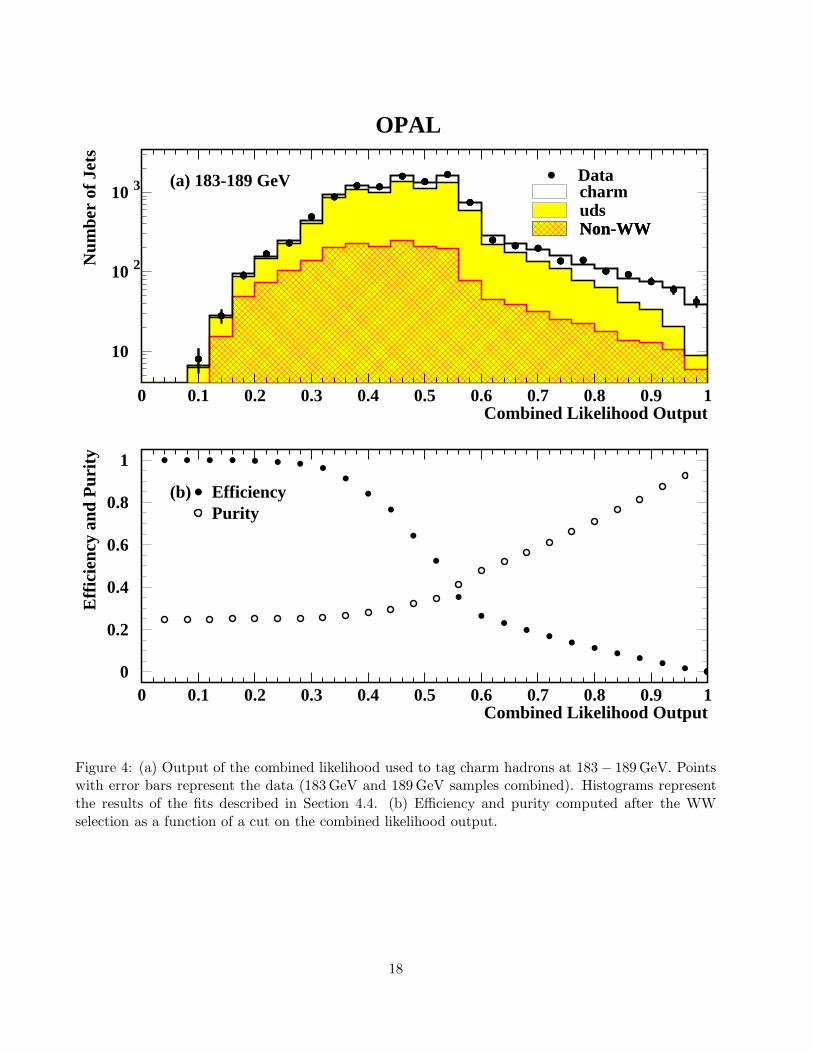
In Figure 4a the combined likelihood output is shown, illustrating the discriminating power betweencharm and light flavoured jets. The efficiency and purity for a particular cut on the combined likelihood

7

output are also depicted in Figure 4b. Table 2 lists the tagging efficiencies for jets in WW andbackground events that result from a cut on the likelihood output at the optimal value of 0.7. Thetagging efficiencies at 189 GeV are slightly higher due to the extra boost of the W bosons. Thesevalues are not directly used to derive RW

c , but are quoted to give an impression of the performance ofthe charm tag.

4.4 Determination of RWc

To extract RWc from the data, a binned maximum likelihood fit is performed to the combined like-

lihood distributions. Template histograms for the charm, light–flavoured, and non–WW backgroundcomponents are produced from the main Monte Carlo samples. They are referred to as the probabilitydensity functions (pdf) for the various components. Using this fitting method improves the statisticalsensitivity of the measurement compared to simply counting the number of jets that pass a cut on thelikelihood output. The function used to fit the data (see Figure 4a) is:

− lnL = −N∑

i=1

ni ln{(1− Fbkg)

(12RW

c Pic + [1− 1

2RWc ]Pi

uds

)+ Fbkg Pi

bkg

}, (1)

with

i: Bin index in the combined likelihood distribution;

ni: Number of jets in the ith bin;

N : Number of bins in the combined likelihood distribution;

Pic: Probability for a charm jet to appear in the ith bin (W → cX pdf);

Piuds: Probability for a uds jet to appear in the ith bin (W → light flavour pdf);

Fbkg: Fraction of background jets;

Pibkg: Probability for a non–WW jet to appear in the ith bin (non–WW background pdf).

The result of the fit for RWc is:

RWc = 0.493 ± 0.090 at 183 GeV

andRW

c = 0.478 ± 0.047 at 189 GeV.

where the errors are statistical only. The χ2/(degree of freedom) of the fits are 17.2/24 at 183 GeVand 35.4/24 at 189 GeV.

4.5 Systematic uncertainties

Since the reference histograms, the efficiencies, and the background for the calculation of RWc were

taken from a Monte Carlo simulation, the analysis depends on the proper modelling of the datadistributions in the simulation. The sources of systematic error are listed in Table 3 and are discussedbelow. Unless otherwise noted, all changes were applied to signal and background Monte Carlosamples.

8

• Hadronisation model: The Pythia Monte Carlo sample, which uses the Lund string fragmenta-tion as implemented in Jetset [5], was compared to a sample generated with Herwig [8], whichuses cluster fragmentation. The samples differ in their parton showering and hadronisation.

• W mass and centre–of–mass energy: As the jet pairing depends on the W mass, MW, and thecentre–of–mass energy,

√s, the analysis was repeated with different W masses and at different

centre–of–mass energies. The W mass was varied by 100 MeV, which covers both the experi-mental uncertainty and the differences between the current world average mass [2] and the valueused in the Monte Carlo. The centre–of–mass energy was varied by the difference between theluminosity–weighted centre–of–mass energies in data and the value of

√s used in the main Monte

Carlo samples.

• Charm fragmentation: At√

s = MZ, the mean scaled energy of weakly decaying charm hadronswas found to be 〈xD(MZ)〉 = 0.484 ± 0.008 [25]. No measurements of this quantity exist for Wdecays, but it is expected to be similar to that in Z decays. The changes in the charm fragmen-tation due to QCD effects were taken from Jetset [5]. To assess the systematic uncertainty,〈xD(MW)〉 was varied by the experimental uncertainty obtained on 〈xD(MZ)〉, i.e. 0.008. Thefragmentation schemes of Peterson [26], Collins and Spiller [27], Kartvelishvili [28] and the Lundgroup [29] were used to assess a possible discrepancy on the shape of the fragmentation function.The largest variation was assigned as the systematic error.

• Background cross–section: In the fit for extracting RWc , the fraction of background was varied

according to the error on the expected fraction of background events from References [11,12].

• Background composition: The various background sources have different probabilities to fake acharm jet. The background composition was varied within the uncertainties given in Table 1.

• Charm hadron fractions: The fractions of the weakly decaying charm hadrons were varied withintheir experimental errors according to Reference [25].

• Light quark composition: The shape of the reference histogram for light–flavoured quarks de-pends on the relative fractions of the u, d, and s jets. The quark flavour fractions were variedaccording to the actual errors on the CKM matrix [2] so that the error covers the effect ofassumptions concerning the CKM matrix elements on the uds template histogram. The num-ber of bottom hadrons from W bosons was also doubled to ensure that the measured RW

c wasinsensitive to the bottom fraction in W decays.

• Vertex reconstruction: The correct modelling of the detector resolution in the Monte Carlosimulation is of paramount importance for the description of the probability to find a secondaryvertex. This was checked by comparing the track parameters between calibration data collectedat

√s ∼ MZ and Monte Carlo simulation. The sensitivity to the vertex reconstruction was

assessed by degrading or improving the tracking resolution in the Monte Carlo. It was foundthat changing the track parameters resolution by±5% covers the range of the observed differencesbetween data and Monte Carlo (see Figure 3a) in the vertex ANN input and output distributions.

• Charm hadron lifetimes: The lifetimes of the weakly decaying charm hadrons were varied withintheir experimental errors according to Reference [2].

• Charm decay multiplicity: The performance of the secondary vertex finder depends on themultiplicity of the final state of the charm hadrons. The relative abundance of 1, 2, 3, 4, 5, and6 prong charm decays was changed in the Monte Carlo within their experimental errors [30].Similarly, the relative abundance of neutral pions was varied in the Monte Carlo within theexperimental errors [30].

9

Source of ∆ RWc

Systematic Error 183 GeV 189 GeVHadronisation Model 0.011 0.012

Centre–of–mass Energy 0.007 0.005Mass of the W Boson 0.004 0.003

Charm Fragmentation Function 0.007 0.007Background Cross-Section 0.006 0.005Background Composition 0.010 0.009Charm Hadron Fractions 0.006 0.007Light Quark Composition 0.007 0.005

Vertex Reconstruction 0.016 0.017Charm Hadron Lifetimes 0.003 0.002Charm Decay Multiplicity 0.010 0.010

Lepton Identification 0.012 0.014Lepton Energy Spectrum 0.003 0.003Branching ratio Br(c → `) 0.006 0.006

Total systematic error 0.032 0.032Statistical error 0.090 0.047Value of RW

c 0.493 0.478

Table 3: Summary of the experimental systematic errors, statistical errors, and central values fromthe binned maximum likelihood fit on RW

c at 183 GeV and 189 GeV.

• Lepton identification: The modelling of the input variables of the ANN for electron identificationhas been intensively studied at LEP1 [22], while the performance of the muon tagging ANN hasbeen investigated using various control samples of calibration data collected at the Z0 resonanceduring each year of LEP2 [23]. The relative error of the efficiency to identify a genuine elec-tron (muon) has been estimated to be 4% (3 %), and the relative error on the probability towrongly identify a hadron as a lepton has been evaluated to be around 16 % (10 %) for electrons(muons) [22, 23]. By studying the dE/dx distributions for electron candidates in calibrationdata taken at the Z0 mass in 1997 and 1998, it was found that a shift of the mean dE/dx of0.04 keV/cm (0.3%) and a scaling by 1% of the dE/dx resolution in data was needed to correcta slight discrepancy between Monte Carlo and data. This effect was also taken into accountin the assignment of the uncertainty on the electron tagging efficiency. The (mis)identificationprobabilities for electrons and muons were varied by reweighting the Monte Carlo events andthe largest resulting change in RW

c was taken as the systematic error. It was verified that thevariation of efficiencies and dE/dx resolution was sufficient to describe the possible differencesbetween data and Monte Carlo (see Figures 3b-c).

• Lepton energy spectrum from semileptonic charm decays: The energy spectrum of the leptonin the rest frame of the weakly decaying charm hadron was reweighted from the spectrumimplemented in Jetset to the ISGW [31] and ACCMM [32] models; the parameters pf and ms

of the ACCMM model were varied in the range recommended in Reference [25].

• Branching ratio Br(c → `): The branching fraction for inclusive charm decays to leptons wasvaried within the range Br(c → `) = 0.098 ± 0.005 [25] by reweighting the Monte Carlo events.

The size of the systematic errors is very similar for the samples at 183 GeV and 189 GeV. The dominantsystematic errors are those associated with the vertex reconstruction and lepton identification.

10

CKM matrix element Value|Vud| 0.9735± 0.0008|Vus| 0.2196± 0.0023

|Vub|/|Vcb| 0.090 ± 0.025|Vcd| 0.224 ± 0.016|Vcb| 0.0402± 0.0019

Table 4: Values of the CKM matrix elements used in the calculation of |Vcs| from RWc . The values are

taken from Reference [2].

5 Results

The result of the charm tag analysis is

RWc = 0.493 ± 0.090 (stat.) ± 0.032 (syst.) at 183 GeV

andRW

c = 0.478 ± 0.047 (stat.) ± 0.032 (syst.) at 189 GeV.

The combined value of RWc obtained at

√s = 183 GeV and 189 GeV is

RWc = 0.481 ± 0.042 (stat.) ± 0.032 (syst.),

where the systematic uncertainties are treated as being fully correlated.

6 Extraction of |Vcs|

It is possible to extract |Vcs| from RWc using the relation

RWc =

|Vcd|2 + |Vcs|2 + |Vcb|2|Vud|2 + |Vus|2 + |Vub|2 + |Vcd|2 + |Vcs|2 + |Vcb|2 , (2)

which leads to

|Vcs| =

√RW

c

1−RWc

(|Vud|2 + |Vus|2 + |Vub|2)− |Vcd|2 − |Vcb|2. (3)

Using the values of the other CKM matrix elements listed in Table 4, one gets

|Vcs| = 0.93 ± 0.08 (stat.) ± 0.06 (syst.) ± 0.004 (CKM),

where the last error is due to the uncertainty on the CKM matrix elements used in the calculation.

A more precise value for |Vcs| can be obtained based on the Standard Model prediction of thedecay width of the W boson to final states containing charm quarks:

Γ (W → cX) =CGFM3

W

6√

2π(|Vcd|2 + |Vcs|2 + |Vcb|2), (4)

with CGFM3W

6√

2π= (705 ± 4)MeV [2] and the color factor C given by [2]

C = 3(

1 +αs (MW)

π+ 1.409

α2s (MW)

π2− 12.77

α3s (MW)

π3

). (5)

11

Γ (W → cX) can be evaluated from RWc using the relation

Γ (W → cX) = RWc Br (W → hadrons) ΓW

tot. (6)

Using the PDG values Br (W → hadrons) = 0.6848 ± 0.0059 and2 ΓWtot = (2.12 ± 0.05)GeV [2]

together with the measurement of RWc presented in this letter, one gets

Γ (W → cX) = [698 ± 61 (stat.) ± 46 (syst.) ± 18 (ext.)]MeV,

where the last error is due to the uncertainties on the external parameters ΓWtot and Br (W → hadrons).

This corresponds to

|Vcd|2 + |Vcs|2 + |Vcb|2 = 0.990 ± 0.087 (stat.) ± 0.065 (syst.) ± 0.026 (ext.).

Subtracting the off–diagonal CKM matrix elements, using the values listed in Table 4, results in

|Vcs| = 0.969 ± 0.045 (stat.) ± 0.034 (syst.) ± 0.013 (ext.) ± 0.004 (CKM),

where the last error is due to the uncertainties on the CKM matrix elements used in the calculation.The determination of |Vcs| from Equations (4) and (6) only involves the CKM matrix elements forthe transition W → cX and well measured parameters such as ΓW

tot and Br (W → hadrons). It istherefore more precise than the method which relies on Equation (3). Both results of |Vcs| presentedhere are compatible with the direct determination from D semielectronic decays which yields |Vcs| =1.04 ± 0.16 [2].

7 Summary

Using data taken with the OPAL detector at LEP at centre–of–mass energies of 183 GeV and 189 GeV,the ratio RW

c = Γ (W → cX)/Γ (W → hadrons) has been measured using a technique based on jetproperties, lifetime information, and leptons from charm decays. The combined result is

RWc = 0.481 ± 0.042 (stat.) ± 0.032 (syst.),

in agreement with the Standard Model expectation of 0.5. This result is consistent with the StandardModel prediction that the W boson couples to up and charm quarks with equal strength and it is inagreement with the recent measurements of DELPHI [34] and ALEPH [35].

Using the results from direct measurements of the other CKM matrix elements, |Vcs| can becalculated from RW

c , yielding |Vcs| = 0.93 ± 0.10. A more precise value for |Vcs| can be derived fromthe measurements of RW

c , Br (W → hadrons), and ΓWtot:

|Vcs| = 0.969 ± 0.058.

This can be compared to a more indirect determination of |Vcs| by OPAL from the ratio of the Wdecay widths to qq and `ν`, which yields |Vcs| = 1.014 ± 0.029 (stat.) ± 0.014 (syst.) [12] under theassumption that the W boson couples with equal strength to quarks and leptons. It should be notedthat the ratio Br (W → qq)/Br (W → `ν`) is not used in the analysis presented here, so that these areindependent determinations of |Vcs|.

2The most precise measurements of ΓWtot are determined from the quantity R = σ (pp→W+X)·Br (W→eν)

σ (pp→Z0+X)·Br (Z0→e+e−). In [33], the

coupling of the W boson to light quarks is needed as input; however, direct measurements of the corresponding CKMmatrix elements are so precise that it introduces a negligible uncertainty on ΓW

tot.

12

Acknowledgements

We particularly wish to thank the SL Division for the efficient operation of the LEP accelerator atall energies and for their continuing close cooperation with our experimental group. We thank ourcolleagues from CEA, DAPNIA/SPP, CE-Saclay for their efforts over the years on the time-of-flightand trigger systems which we continue to use. In addition to the support staff at our own institutionswe are pleased to acknowledge theDepartment of Energy, USA,National Science Foundation, USA,Particle Physics and Astronomy Research Council, UK,Natural Sciences and Engineering Research Council, Canada,Israel Science Foundation, administered by the Israel Academy of Science and Humanities,Minerva Gesellschaft,Benoziyo Center for High Energy Physics,Japanese Ministry of Education, Science and Culture (the Monbusho) and a grant under the Mon-busho International Science Research Program,Japanese Society for the Promotion of Science (JSPS),German Israeli Bi-national Science Foundation (GIF),Bundesministerium fur Bildung und Forschung, Germany,National Research Council of Canada,Research Corporation, USA,Hungarian Foundation for Scientific Research, OTKA T-029328, T023793 and OTKA F-023259.

References

[1] N. Cabibbo, Phys. Rev. Lett. 10 (1963) 531;M. Kobayashi and T. Maskawa, Prog. Theor. Phys. 49 (1973) 652.

[2] D.E.. Groom et al., Eur. Phys. J. C15 (2000) 1.

[3] OPAL Collaboration, K. Ahmet et al., Nucl. Instr. Meth. A305 (1991) 275;P.P. Allport et al., Nucl. Instr. Meth. A324 (1993) 34;P.P. Allport et al., Nucl. Instr. Meth. A346 (1994) 476;S. Anderson et al., Nucl. Instr. Meth. A403 (1998) 326.

[4] M. Skrzypek et al., Comput. Phys. Commun. 94 (1996) 216;M. Skrzypek et al., Phys. Lett. B372 (1996) 289.

[5] T. Sjostrand, Comput. Phys. Commun. 39 (1986) 347;T. Sjostrand and H.–U. Bengtsson, Comput. Phys. Commun. 43 (1987) 367.

[6] J. Allison et al., Nucl. Instr. Meth. A317 (1992) 47.

[7] T. Sjostrand, Comput. Phys. Commun. 82 (1994) 74.

[8] G. Marchesini et al., Comput. Phys. Commun. 67 (1992) 465.

[9] F.A. Berends, R. Pittau and R. Kleiss, Comput. Phys. Commun. 85 (1995) 437.

[10] J. Fujimoto et al., Comput. Phys. Commun. 100 (1997) 128.

13

[11] OPAL Collaboration, G. Abbiendi et al., Eur. Phys. J. C8 (1999) 191.

[12] OPAL Collaboration, W+W− Production Cross Section and W Branching Fractions in e+e−

Collisions at 189 GeV, OPAL PR321, CERN-EP-2000-101 (2000), Submitted to Phys. Lett. B.

[13] S. Catani et al., Phys. Lett. B269 (1991) 432.

[14] OPAL Collaboration, G. Abbiendi et al., Phys. Lett. B453 (1999) 138.

[15] OPAL Collaboration, Measurement of the Mass and Width of the W Boson in e+e− Collisionsat 189,GeV, OPAL PR320, CERN-EP-2000-099 (2000), Submitted to Phys. Lett. B.

[16] OPAL Collaboration, G. Abbiendi et al., Phys. Lett. B453 (1999) 153.

[17] OPAL Collaboration, K. Ackerstaff et al., Z. Phys. C74 (1997) 1.

[18] OPAL Collaboration, K. Ackerstaff et al., Eur. Phys. J. C1 (1998) 439.

[19] C. Peterson, T. Rognvaldsson and L. Lonnblad, JETNET 3.0 - A Versatile Artificial NeuralNetwork Package, LU–TP–93–29, CERN–TH.7135/94.

[20] ALEPH Collaboration, D. Buskulic et al., Phys. Lett. B313 (1993) 535.

[21] OPAL Collaboration, G. Alexander et al., Z. Phys. C70 (1996) 357.

[22] OPAL Collaboration, G. Abbiendi et al., Eur. Phys. J. C8 (1999) 217.

[23] OPAL Collaboration, Measurements of Rb, AbFB, and Ac

FB in e+e− Collisions at 130–189 GeV,CERN-EP/99-170 (1999), Submitted to Eur. Phys. J. C.

[24] D. Karlen, Comp. in Phys. 12:4 (1998) 380.

[25] ALEPH, DELPHI, L3, and OPAL Collaborations: Nucl. Instr. Meth. A378 (1996) 101;Updates of the recommendations are given in the LEP electroweak working group: Input Pa-rameters for the LEP Electroweak Heavy Flavour Results for Summer 1998 Conferences, internalnote LEPHF/98–01 (URL: http://www.cern.ch/LEPEWWG/heavy/).

[26] C. Peterson, D. Schlatter, I. Schmitt, and P.M. Zerwas, Phys. Rev. D27 (1983) 105.

[27] P. Collins and T. Spiller, J. Phys. G11 (1985) 1289.

[28] V.G. Kartvelishvili, A.K. Likhoded and V.A. Petrov, Phys. Lett. B78 (1978) 615.

[29] B. Anderson, G. Gustafson and B. Soderberg, Z. Phys. C20 (1983) 317.

[30] Mark III Collaboration, D. Coffman et al., Phys. Lett. B263 (1991) 135.

[31] N. Isgur, D. Scora, B. Grinstein, M.B. Wise, Phys. Rev. D39 (1989) 799;N. Isgur and M.B. Wise, Phys. Rev. D41 (1990) 151.

[32] G. Altarelli et al., Nucl. Phys. B208 (1982) 365.

[33] D0 Collaboration, S. Abachi et al., Phys. Rev. Lett. 75 (1995) 1456;CDF Collaboration, F. Abe et al., Phys. Rev. D52 (1995) 2624.

[34] DELPHI Collaboration, P. Abreu et al., Phys. Lett. B439 (1998) 209.

[35] ALEPH Collaboration, R. Barate et al., Phys. Lett. B465 (1999) 349.

14

OPAL

1

10

10 2

10 3

0 2.5 5 7.5 10 12.5 15 17.5 20 22.5 25Decay Length Significance

Num

ber

of V

ertic

es

DatacharmudsNon-WWNon-WW

0255075

100125150175200225

0 0.1 0.2 0.3 0.4 0.5 0.6 0.7 0.8 0.9 1Vertex Joint Probability

Num

ber

of V

ertic

es

(a) 183-189 GeV

(b) 183-189 GeV DatacharmudsNon-WWNon-WW

Figure 1: Distributions of the most sensitive input variables of the vertex ANN at√

s = 183−189 GeV:(a) decay length significance L/σL and (b) primary vertex joint probability. Points with error barsrepresent the data (183 GeV and 189 GeV samples combined). Histograms represent the Monte Carloexpectation.

15

OPAL

10

10 2

10 3

10 4

0 0.1 0.2 0.3 0.4 0.5 0.6 0.7 0.8 0.9 1Vertex ANN Output

Num

ber

of J

ets

DatacharmudsNon-WWNon-WW

10

10 2

10 3

10 4

0 0.1 0.2 0.3 0.4 0.5 0.6 0.7 0.8 0.9 1Lepton Likelihood Output

Num

ber

of J

ets

(a) 183-189 GeV

(b) 183-189 GeV DatacharmudsNon-WWNon-WW

Figure 2: Distributions of (a) the vertex ANN output and (b) the likelihood output of the lepton tagat√

s = 183 − 189 GeV. Points with error bars represent the data (183 GeV and 189 GeV samplescombined). Histograms show the results of the fits to the combined likelihood described in Section 4.4.If no vertex or lepton tag information is available, the corresponding variable is assigned the value ofzero.

16

OPAL

10

10 2

10 3

10 4

-15 -10 -5 0 5 10 15 20 25Decay Length Significance

Num

ber

of V

ertic

e C

andi

date

s

Z Calibration DataMonte Carlo ExpectationSystematic Variation

0200400600800

10001200140016001800

-2 0 2 4Normalised dE/dx

Num

ber

of E

lect

ron

Can

dida

tes

(c)(b)

(a)

0

500

1000

1500

2000

2500

3000

3500

0 0.5 1 1.5 2E/p

Num

ber

of E

lect

ron

Can

dida

tes

Figure 3: Comparison of discriminating variables between calibration data taken at the Z0 resonanceand Monte Carlo prediction. Points with error bars represent data from the Z0 calibration runs.Histograms show the expectation from the Monte Carole simulation. (a) Decay length significanceL/σL for data and Monte Carlo. The dotted line shows the effect of the ±5 % variation of the trackingresolution used to assess the systematic uncertainty on the vertex tag. (b) E/p and (c) normaliseddE/dx for electron candidates from data and Monte Carlo. In these plots, electrons must satisfy thepre-selection described in the text and have an electron ANN output greater than 0.5. The dottedlines show how the variation of the detection (mis)identification and resolution for electron candidatesaffects the E/p and dE/dx distributions.

17

OPAL

10

10 2

10 3

0 0.1 0.2 0.3 0.4 0.5 0.6 0.7 0.8 0.9 1Combined Likelihood Output

Num

ber

of J

ets

DatacharmudsNon-WWNon-WW

0

0.2

0.4

0.6

0.8

1

0 0.1 0.2 0.3 0.4 0.5 0.6 0.7 0.8 0.9 1

EfficiencyPurity

(b)

(a) 183-189 GeV

Combined Likelihood Output

Effi

cien

cy a

nd P

urity

Figure 4: (a) Output of the combined likelihood used to tag charm hadrons at 183− 189 GeV. Pointswith error bars represent the data (183 GeV and 189 GeV samples combined). Histograms representthe results of the fits described in Section 4.4. (b) Efficiency and purity computed after the WWselection as a function of a cut on the combined likelihood output.

18