A Local Frequency Analysis of Light Scattering and Absorption

A Local Frequency Analysis of Light Scattering and AbsorptionLAURENT BELCOURManao†, Inria Bordeaux Sud-OuestandKAVITA BALACornell UniversityandCYRIL SOLERMaverick, Inria Rhone-Alpes

Rendering participating media requires significant computation, but theeffect of volumetric scattering is often eventually smooth. This paper pro-poses an innovative analysis of absorption and scattering of local light fieldsin the Fourier domain, and derives the corresponding set of operators on thecovariance matrix of the power spectrum of the light field. This analysisbrings an efficient prediction tool for the behavior of light along a light pathin participating media. We leverage this analysis to derive proper frequencyprediction metrics in 3D by combining per-light path information in thevolume.

We demonstrate the use of these metrics to significantly improve the con-vergence of a variety of existing methods for the simulation of multiple scat-tering in participating media. Firstly, we propose an efficient computationof second derivatives of the fluence, to be used in methods like irradiancecaching. Secondly, we derive proper filters and adaptive sample densities forimage-space adaptive sampling and reconstruction. Thirdly, we propose anadaptive sampling for the integration of scattered illumination to the cam-era. Finally, we improve the convergence of progressive photon beams bypredicting where the radius of light gathering can stop decreasing. Lightpaths in participating media can be very complex. Our key contribution isto show that analyzing local light fields in the Fourier domain reveals theconsistency of illumination in such media, and provides a set of simple anduseful rules to be used to accelerate existing global illumination methods.

Categories and Subject Descriptors: I.3.7 [Computer Graphics]: Three-Dimensional Graphics and Realism—Raytracing

Additional Key Words and Phrases: global illumination, participating me-dia, adaptive sampling, frequency analysis

†Inria - LP2N (CNRS, Univ. Bordeaux, IOGS) - LaBRI (CNRS, Univ. Bor-deaux)Permission to make digital or hard copies of part or all of this work forpersonal or classroom use is granted without fee provided that copies arenot made or distributed for profit or commercial advantage and that copiesshow this notice on the first page or initial screen of a display along withthe full citation. Copyrights for components of this work owned by othersthan ACM must be honored. Abstracting with credit is permitted. To copyotherwise, to republish, to post on servers, to redistribute to lists, or to useany component of this work in other works requires prior specific permis-sion and/or a fee. Permissions may be requested from Publications Dept.,ACM, Inc., 2 Penn Plaza, Suite 701, New York, NY 10121-0701 USA, fax+1 (212) 869-0481, or [email protected]© YYYY ACM 0730-0301/YYYY/14-ARTXXX $10.00

DOI 10.1145/XXXXXXX.YYYYYYYhttp://doi.acm.org/10.1145/XXXXXXX.YYYYYYY

1. INTRODUCTION

Rendering participating media is challenging because of the highcost of simulating scattering events. But participating media mostlyblur out details, and decrease the contrast of images: some imageregions appear almost locally constant, and light beams are practi-cally constant in the direction of light propagation. In this paper weintroduce a new frequency analysis of local light fields in partici-pating media. We show the effect that volumetric scattering has onlowering frequency content and contrast. We derive the associatedtheoretical framework and provide tools to optimize participatingmedia rendering algorithms using the frequency content of lighttransport.

Scattering is a long standing problem in computer graphicswhere a range of techniques, with varying trade-offs between per-formance and accuracy, have been proposed to simulate the inter-action of light with participating media. Unbiased methods suchas path tracing [Lafortune and Willems 1993] and Metropolislight transport [Veach and Guibas 1997] provide accuracy, but of-ten at a prohibitive cost. Photon mapping based approaches han-dle participating media [Jensen and Christensen 1998; Knaus andZwicker 2011] with different trade-offs. Methods such as PhotonBeams [Jarosz et al. 2011] efficiently simulate low order scatter-ing, relying on the accumulation of illumination primitives (e.g.,points or beams) to compute images. While some approaches ex-ploit the lower frequency nature of lighting in participating media,to our knowledge, there is no existing literature on a priori fre-quency analysis of local light fields in volume transport.

For non-volumetric surface-based rendering, Durand etal. [2005] introduced a frequency analysis of light transport. Weextend this framework to characterize the behavior, in the Fourierdomain, of light traveling and scattering inside participating media.Methods exist that use the Fourier transform as a global transformoperator in 3D to decouple the frequencies in the scatteringequation [Ishimaru 1997]. Instead, our extension to the frequencyanalysis framework applies to 4D local light fields, along lightpaths in the medium.

We build on covariance analysis [Belcour et al. 2013], an effi-cient and practical representation of the covariance matrix of thefrequency spectrum of the local light field. It was used to acceler-ate the rendering of motion and defocus blur. The covariance ma-trix representation conveys the required information on the Fouriertransform of the light field, at a very small cost, making it tractablefor path-tracing.

In this paper, we extend the covariance representation to globalillumination in participating media, including multiple scattering.We show that our new formulae for participating media fit nicely in

ACM Transactions on Graphics, Vol. VV, No. N, Article XXX, Publication date: Month YYYY.

hal-0

0957

242,

ver

sion

1 -

14 M

ar 2

014

Author manuscript, published in "ACM Transactions on Graphics to appear (2014)"

http://hal.inria.fr/hal-00957242

http://hal.archives-ouvertes.fr

2 •

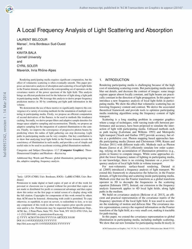
(a) Our frequency estimate combined with (b) Predicted 3D covariance (c) Image space filters (d) Reference (Prog. Photon Beams, 4h44min)Progressive Photon Beams (25 min) of fluence spectrum & Camera rays sample density Inset: Equal time comparison (25min)

Fig. 1. We propose a frequency analysis of light transport in participating media, a broad theoretical tool that allows improvements in a wide variety ofalgorithms. From the predicted 3D covariance of the fluence in the Fourier domain (b), we derive three different sampling metrics in the 3D volume. We presentmultiple example uses of these metrics: to improve image-space adaptive sampling density and reconstruction, we provide sampling density and reconstructionfilters (c-top); to improve light integration along camera rays, we evaluate a required number of samples along those rays (c-bottom); to improve progressivephoton beams, we derive the optimal reconstruction radius based on the frequency content (a and d). In order to ease comparisons, we scaled the covariancegraphs (b), and increased the luminosity of insets (d). This scene is composed of a pumpkin modeled by user Mundomupa of blendswap.com provided undercreative common license CC-BY, and of a house front modeled by Jeremy Birn.

the existing framework when the medium is not optically thick (asin subsurface scattering). We use the covariance information of thelocal light field spectrum in 4D along light paths to predict the 3Dcovariance of the windowed spectrum of fluence in volumes withparticipating media. We propose four application scenarios wherethis quantity proves useful (see Figure 1). The contributions of thispaper are:

—A local analysis of scattering and absorption in the Fourier do-main along a light path, in heterogeneous participating media.The model is compatible with multiple scattering.

—A compact representation of attenuation and scattering in theFourier domain, using covariance matrices.

—The combination of covariance from many light paths in themedium into usable sampling metrics in 3D.

—Four different computation scenarios that benefit from our anal-ysis: computation of second derivatives of the fluence; imagespace adaptive sampling and reconstruction; adaptive samplingof scattered illumination along rays from the camera; and pro-gressive photon beams.

Note that the term “spectral analysis” usually has multiple mean-ings; it is sometimes used to refer to the eigenanalysis of linearoperators. In this paper the term spectrum refers to the frequencyspectrum of the Fourier transform of light fields.

2. PREVIOUS WORK

We categorize related work into research on the frequency analy-sis of light transport, and on the volume rendering of participatingmedia.

2.1 Fourier domain methods for scattering.

In these methods, the Fourier transform is used as a tool for solv-ing the scattering equation at once in the entire domain [Duderstadtand Martin 1979; Ishimaru 1997]. Some methods use a differentbasis for certain dimensions, such as the Chebychev basis [Kimand Moscoso 2003], or spherical harmonics [Dave 1970]. Thesemethods in general depend on a combination of very specific con-straints: infinite or spherical domains [Dave and Gazdag 1970], pe-riodic boundary conditions [Ritchie et al. 1997], isotropic scatter-ing functions [Rybicki 1971], and mostly homogeneous scatteringfunctions. These conditions make such methods not very suitableto computer generated images where the constraints of uniformityand periodicity can hardly be satisfied.

Our approach is fundamentally different: we use the Fouriertransform as a local tool in the 4D ray space to predict bandwidth—as opposed to globally solving the equations—which allows us tohandle non homogeneous participating media.

2.2 Volume rendering.

The field of rendering participating media has a long history. Vol-ume rendering based on ray tracing techniques was first proposedfor forward path tracing integration [Kajiya and Von Herzen 1984].It has been expanded afterwards to other integration schemes:Lafortune and Willems [1996] extended bidirectional path tracing;Pauly et al. [2000] adapted Metropolis for participating media. Pho-ton mapping [Jensen and Christensen 1998] has been shown to beefficient in generating high frequency light patterns such as caus-tics. Cerezo et al. [2005] surveys the state-of-the-art, though it is abit dated.

Recently, various extensions to photon mapping and progres-sive photon mapping use photon beams, rather than point samplingalong rays, to greatly improve the performance of volume render-ing [Jarosz et al. 2008; Jarosz et al. 2011; Jarosz et al. 2011; Knaus


hal-0

0957

242,

ver

sion

1 -

14 M

ar 2

014

• 3

and Zwicker 2011]. These methods however, remain unaware ofimage complexity, and rely on an accumulation of illuminationprimitives (e.g., points or beams) to compute an image that willeventually be very smooth.

Several virtual point light (VPL)-based algorithms for volumet-ric rendering trade-off quality and performance. Light cuts andvariants [Walter et al. 2005; Walter et al. 2006; Walter et al. 2012]achieve scalable rendering of complex lighting with many VPLsfor motion blur, depth of field, and volumetric media (including fororiented media [Jakob et al. 2010]). These scalable approaches cou-ple error bounded approximations with simple perceptual metrics.For interactive VPL rendering of participating media, Engelhardt etal. [2010] introduce a GPU-friendly bias compensation algorithm.Novak et al. [2012] spread the energy of virtual lights along bothlight and camera rays, significantly diminishing noise caused bysingularities.

Multiple approaches aim at efficiently computing low-order scat-tering in refractive media. Walter et al. [2009] compute single scat-tering in refractive homogeneous media with triangle boundaries.Ihrke et al. [2007] solve the eikonal equation with wavefront trac-ing for inhomogeneous media with varying refractive indices andSun et al. [2010] develop a line gathering algorithm to integratecomplex multiple reflection/refraction and single scattering volu-metric effects for homogeneous media.

2.3 Efficient sampling and reconstruction methods

Some works perform adaptive sampling or local filtering usingheuristics based on the frequency of light transport, without ex-plicitly computing frequency information. Adaptive sampling forsingle scattering [Engelhardt and Dachsbacher 2010] permits re-sampling when detecting an occlusion. This approach finds epipo-lar lines, sparsely samples and interpolates along these lines, butfinds occlusion boundaries to preserve high frequency details. Anepipolar coordinate system [Baran et al. 2010; Chen et al. 2011] al-lows to interactively compute single scattering in volumetric mediaby exploiting the regularity of the visibility function.

The structure of the light field [Levoy and Hanrahan 1986;Gortler et al. 1986] can be exploited to perform adaptive samplingor reconstruction. For surface radiance computation, Lehtinen etal. [2011] exploits anisotropy in the temporal light field to effi-ciently reuse samples between pixels, and perform visibility-awareanisotropic reconstruction to indirect illumination, ambient occlu-sion and glossy reflections. Ramamoorthi et al. [2012] derived atheory of Monte Carlo visibility sampling to decide on the bestsampling strategies depending on a particular geometric configura-tion. Mehta et al. [2012] derives the sampling rates and filter sizesto reconstruct soft shadows from a theoretical analysis to consideraxis-aligned filtering.

Irradiance caching methods [Jarosz et al. 2008] inherently per-form filtering in the space of the irradiance by looking at the ir-radiance gradient. For example, Ribardiere et al. [2011] performadaptive irradiance caching for volumetric rendering. They predictvariations of the irradiance and map an ellipsoid to define the non-variation zone with respect to a local frame.

2.4 Frequency analysis of light transport.

In their frequency analysis of light transport, Durand et al. [2005]studied the frequency response of the radiance function to variousradiative transport phenomena (such as transport, occlusion and re-flection). Other works on this subject [Egan et al. 2009; Soler et al.2009; Belcour and Soler 2011; Bagher et al. 2012] have enrichedthe number of effects to be studied (motion, lens) and showed that

filtering and adaptive sampling methods can benefit from frequencyanalysis. Yet, some radiative phenomena have not been studied inthis framework, including refraction and scattering. We aim to fill apart of this gap by bringing comprehension of the frequency equiv-alent of volume scattering and attenuation operators, and showingthe usefulness of such analysis with a few practical applications.

A frequency analysis has been carried out for shadows specifi-cally by Egan et al.in 4D to build sheared reconstruction filters forcomplex visibility situations [Egan et al. 2011], or in the case ofocclusion by distant illumination [Egan et al. 2011].

3. BACKGROUND: COVARIANCE OF LOCALSPECTRUM

Our ultimate goal is to provide a general, efficient tool for predict-ing the variations of the illumination, at different stages of the cal-culation of global illumination, so as to make sampling and recon-struction methods the most efficient possible. In prior work [Bel-cour et al. 2013], it was demonstrated that the covariance of thespectrum of the local light field along rays does this job. In this pa-per, we perform the mathematical analysis to extend this approachto multiple scattering in participating media. This section recallsthe basics about local light fields, Fourier analysis of light transportand the covariance representation of the spectrum as background.

3.1 Local light fields

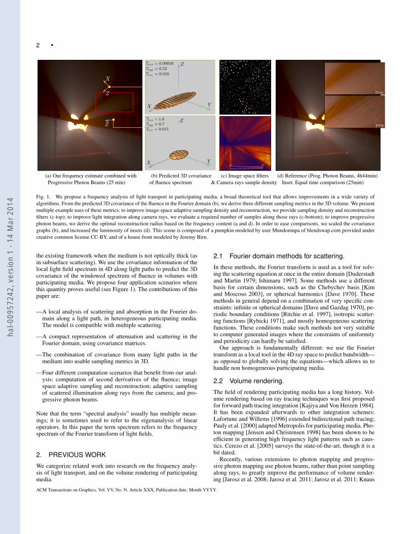
We call the local light field the 4D field of radiance in the 4D neigh-borhood of a ray. Our space of study is the 4D domain of tangen-tial positions around a central ray [Igehy 1999; Wand and Straßer2003]. It is parameterized by two spatial and two angular coordi-nates, defined with respect to the plane orthogonal to the ray at a3D position x (See Figure 2).

Fig. 2. Parameterization of a local radiance light field around a ray of di-rection ω. We use δu, δv as the transverse spatial coordinates of the ray andδθ, δφ as its angular coordinates.

3.2 Fourier analysis

Durand et al. analyzed the various effects a local light field un-dergoes along a light path [Durand et al. 2005]. They showed thatthe effect of light transport operators such as reflection, free spacetransport, and occlusion, all correspond to simple operators on theFourier spectrum of the light field. These operators and their equiv-alent operator in the Fourier domain are listed in Table I.


hal-0

0957

242,

ver

sion

1 -

14 M

ar 2

014

4 •

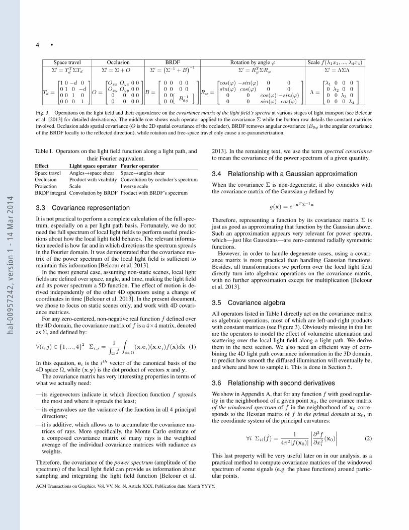
Space travel Occlusion BRDF Rotation by angle ϕ Scale f(λ1x1, ..., λ4x4)

Σ′ = TTd ΣTd Σ′ = Σ +O Σ′ =(Σ−1 +B

)−1Σ′ = RTϕΣRϕ Σ′ = ΛΣΛ

Td =

1 0 −d 00 1 0 −d0 0 1 00 0 0 1

O =

Oxx Oyx 0 0Oxy Oyy 0 0

0 0 0 00 0 0 0

B =

0 00 0

0 00 0

0 00 0

[B−1θφ

]Rϕ =

cos(ϕ) −sin(ϕ) 0 0sin(ϕ) cos(ϕ) 0 0

0 0 cos(ϕ) −sin(ϕ)0 0 sin(ϕ) cos(ϕ)

Λ =

λ1 0 0 00 λ2 0 00 0 λ3 00 0 0 λ4

Fig. 3. Operations on the light field and their equivalence on the covariance matrix of the light field’s spectra at various stages of light transport (see Belcouret al. [2013] for detailed derivations). The middle row shows each operator applied to the covariance Σ while the bottom row details the constant matricesinvolved. Occlusion adds spatial covariance (O is the 2D spatial covariance of the occluder), BRDF removes angular covariance (Bθφ is the angular covarianceof the BRDF locally to the reflected direction), while rotation and free-space travel only cause a re-parameterization.

Table I. Operators on the light field function along a light path, andtheir Fourier equivalent.

Effect Light space operator Fourier operatorSpace travel Angles→space shear Space→angles shearOcclusion Product with visibility Convolution by occluder’s spectrumProjection Scale Inverse scaleBRDF integral Convolution by BRDF Product with BRDF’s spectrum

3.3 Covariance representation

It is not practical to perform a complete calculation of the full spec-trum, especially on a per light path basis. Fortunately, we do notneed the full spectrum of local light fields to perform useful predic-tions about how the local light field behaves. The relevant informa-tion needed is how far and in which directions the spectrum spreadsin the Fourier domain. It was demonstrated that the covariance ma-trix of the power spectrum of the local light field is sufficient tomaintain this information [Belcour et al. 2013].

In the most general case, assuming non-static scenes, local lightfields are defined over space, angle, and time, making the light fieldand its power spectrum a 5D function. The effect of motion is de-rived independently of the other 4D operators using a change ofcoordinates in time [Belcour et al. 2013]. In the present document,we chose to focus on static scenes only, and work with 4D covari-ance matrices.

For any zero-centered, non-negative real function f defined overthe 4D domain, the covariance matrix of f is a 4×4 matrix, denotedas Σ, and defined by:

∀(i, j) ∈ 1, ..., 42 Σi,j =1∫Ωf

∫x∈Ω

(x.ei)(x.ej)f(x)dx (1)

In this equation, ei is the ith vector of the canonical basis of the4D space Ω, while (x.y) is the dot product of vectors x and y.

The covariance matrix has very interesting properties in terms ofwhat we actually need:

—its eigenvectors indicate in which direction function f spreadsthe most and where it spreads the least;

—its eigenvalues are the variance of the function in all 4 principaldirections;

—it is additive, which allows us to accumulate the covariance ma-trices of rays. More specifically, the Monte Carlo estimate ofa composed covariance matrix of many rays is the weightedaverage of the individual covariance matrices with radiance asweights.

Therefore, the covariance of the power spectrum (amplitude of thespectrum) of the local light field can provide us information aboutsampling and integrating the light field function [Belcour et al.

2013]. In the remaining text, we use the term spectral covarianceto mean the covariance of the power spectrum of a given quantity.

3.4 Relationship with a Gaussian approximation

When the covariance Σ is non-degenerate, it also coincides withthe covariance matrix of the Gaussian g defined by

g(x) = e−xT Σ−1x

Therefore, representing a function by its covariance matrix Σ isjust as good as approximating that function by the Gaussian above.Such an approximation appears very relevant for power spectra,which—just like Gaussians—are zero-centered radially symmetricfunctions.

However, in order to handle degenerate cases, using a covari-ance matrix is more practical than handling Gaussian functions.Besides, all transformations we perform over the local light fielddirectly turn into algebraic operations on the covariance matrix,with no further approximation except for multiplication [Belcouret al. 2013].

3.5 Covariance algebra

All operators listed in Table I directly act on the covariance matrixas algebraic operations, most of which are left-and-right productswith constant matrices (see Figure 3). Obviously missing in this listare the operators to model the effect of volumetric attenuation andscattering over the local light field along a light path. We derivethem in the next section. We also need an efficient way of com-bining the 4D light path covariance information in the 3D domain,to predict how smooth the diffused illumination will eventually be,and where and how to sample it. This is done in Section 5.

3.6 Relationship with second derivatives

We show in Appendix A, that for any function f with good regular-ity in the neighborhood of a given point x0, the covariance matrixof the windowed spectrum of f in the neighborhood of x0 corre-sponds to the Hessian matrix of f in the primal domain at x0, inthe coordinate system of the principal curvatures:

∀i Σii(f) =1

4π2|f(x0)|

∣∣∣∣∂2f

∂x2i

(x0)

∣∣∣∣ (2)

This last property will be very useful later on in our analysis, as apractical method to compute covariance matrices of the windowedspectrum of some signals (e.g. the phase functions) around partic-ular points.


hal-0

0957

242,

ver

sion

1 -

14 M

ar 2

014

• 5

4. FOURIER ANALYSIS FOR PARTICIPATING MEDIA

In this section, we extend the frequency analysis of light transportto participating media. We follow a light path, bouncing possiblymultiple times, into the medium. Our model is therefore compati-ble with multiple scattering. We derive the equations to model theeffect of two operators over the frequency spectrum of the locallight field around this light path: absorption and scattering. We firstperform a first order expansion of the phenomena. We then studythe Fourier equivalent of the two operators, and show how to ex-press them using algebraic operations on the spectral covariancematrices of the light field. Table II summarizes our notations.

Table II. Definitions and notations used in the paper.δu, δv, δθ, δφ Spatial and angular local coordinatesl(δu, δv, δθ, δφ) local light field functionΩu,Ωv ,Ωθ,Ωφ Spatial and angular variables in Fourier spacel(Ωu,Ωv ,Ωθ,Ωφ) Fourier spectrum of the local light fieldΣ 4D covariance of the local light field spectrumΓ 3D covariance of windowed spectrum of fluenceδt Coordinate along the central direction of travelκ(x, y, z) Volumetric absorption at 3D position (x, y, z)κuv(u, v) Volumetric absorption in plane orthogonal to a rayω,ωi, ωs directions of light (general, incident, scattered)ρ(ωi, ωs) phase function for directions ωi, ωsρ(δθ, δφ) phase function around ωi, ωs, i.e. ρ(0, 0) = ρ(ωi, ωs)

ρg Henyey-Greenstein function with parameter gα Finite angle for scattered direction⊗ΩuΩv Convolution operator in the Fourier Ωu,Ωv plane

Although the behavior of individual light paths in participatingmedia is potentially complicated, we will show that in the Fourierdomain, absorption acts like visibility, and scattering acts like re-flectance. Not only does this fit elegantly into the existing frame-work, but it also results in a very simple frequency prediction toolfor efficiently rendering participating media.

4.1 Volumetric absorption

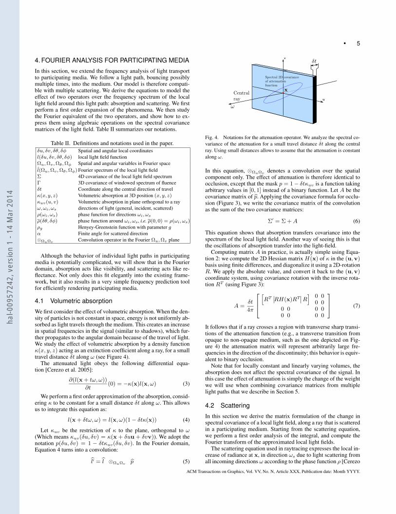
We first consider the effect of volumetric absorption. When the den-sity of particles is not constant in space, energy is not uniformly ab-sorbed as light travels through the medium. This creates an increasein spatial frequencies in the signal (similar to shadows), which fur-ther propagates to the angular domain because of the travel of light.We study the effect of volumetric absorption by a density functionκ(x, y, z) acting as an extinction coefficient along a ray, for a smalltravel distance δt along ω (see Figure 4).

The attenuated light obeys the following differential equa-tion [Cerezo et al. 2005]:

∂(l(x + tω, ω))

∂t(0) = −κ(x)l(x, ω) (3)

We perform a first order approximation of the absorption, consid-ering κ to be constant for a small distance δt along ω. This allowsus to integrate this equation as:

l(x + δtω, ω) = l(x, ω)(1− δtκ(x)) (4)

Let κuv be the restriction of κ to the plane, orthogonal to ω(Which means κuv(δu, δv) = κ(x + δuu + δvv)). We adopt thenotation p(δu, δv) = 1 − δtκuv(δu, δv). In the Fourier domain,Equation 4 turns into a convolution:

l′ = l ⊗ΩuΩv p (5)

Fig. 4. Notations for the attenuation operator. We analyze the spectral co-variance of the attenuation for a small travel distance δt along the centralray. Using small distances allows to assume that the attenuation is constantalong ω.

In this equation, ⊗ΩuΩv denotes a convolution over the spatialcomponent only. The effect of attenuation is therefore identical toocclusion, except that the mask p = 1− δtκuv is a function takingarbitrary values in [0, 1] instead of a binary function. Let A be thecovariance matrix of p. Applying the covariance formula for occlu-sion (Figure 3), we write the covariance matrix of the convolutionas the sum of the two covariance matrices:

Σ′ = Σ +A (6)

This equation shows that absorption transfers covariance into thespectrum of the local light field. Another way of seeing this is thatthe oscillations of absorption transfer into the light-field.

Computing matrix A in practice, is actually simple using Equa-tion 2: we compute the 2D Hessian matrix H(x) of κ in the (u,v)basis using finite differences, and diagonalize it using a 2D-rotationR. We apply the absolute value, and convert it back to the (u,v)coordinate system, using covariance rotation with the inverse rota-tion RT (using Figure 3):

A =δt

4π

[RT∣∣RH(x)RT

∣∣R] 0 00 0

0 00 0

0 00 0

(7)

It follows that if a ray crosses a region with transverse sharp transi-tions of the attenuation function (e.g., a transverse transition fromopaque to non-opaque medium, such as the one depicted on Fig-ure 4) the attenuation matrix will represent arbitrarily large fre-quencies in the direction of the discontinuity; this behavior is equiv-alent to binary occlusion.

Note that for locally constant and linearly varying volumes, theabsorption does not affect the spectral covariance of the signal. Inthis case the effect of attenuation is simply the change of the weightwe will use when combining covariance matrices from multiplelight paths that we describe in Section 5.

4.2 Scattering

In this section we derive the matrix formulation of the change inspectral covariance of a local light field, along a ray that is scatteredin a participating medium. Starting from the scattering equation,we perform a first order analysis of the integral, and compute theFourier transform of the approximated local light fields.

The scattering equation used in raytracing expresses the local in-crease of radiance at x, in direction ωs due to light scattering fromall incoming directions ω according to the phase function ρ [Cerezo


hal-0

0957

242,

ver

sion

1 -

14 M

ar 2

014

6 •

et al. 2005]:

∂(l(x + tωs, ωs))

∂t(0) =

κs4π

∫ω∈S2

ρ(ω, ωs) l(x, ω)dω (8)

Integrating for a small traveling distance δt, we obtain:

l(x+δtωs, ωs) = l(x, ωs)+δtκs4π

∫ω∈S2

ρ(ω, ωs) l(x, ω)dω (9)

When performing Monte-Carlo rendering in participating media,the sum on the right is handled by deciding with Russian Roulettewhether the light path scatters or not. Consequently, to study scat-tering along a light path that is known to scatter, we need to dealwith the integral term of the above equation only.

4.2.1 Scattering the local light fields. We study the implicationof this equation in the 4D neighborhood of a couple of directions ωiand ωs, making a finite angle α (In other words, cosα = ωi.ωs).We derive the scattering equation for small perturbations aroundthe incoming and outgoing directions.

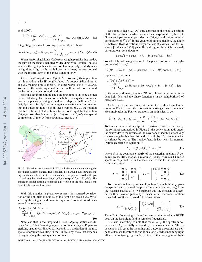
We consider the incoming and outgoing light fields to be definedin correlated angular frames, for which the first angular componentlies in the plane containing ωs and ωi, as depicted in Figure 5. Let(δθ, δφ) and (δθ′, δφ′) be the angular coordinates of the incom-ing and outgoing light fields in these frames, Rδθ,δφ the rotationthat turns the central direction into the local light field direction(δθ, δφ). We also denote by (δu, δv) (resp. δu′, δv′) the spatialcomponents of the 4D frame around ωi (resp. ωs).

Fig. 5. Notations for scattering in 3D, with the input and output angularcoordinate systems aligned. The local light field around the central incom-ing direction ωi (resp. scattered direction ωs) is parameterized with spa-tial and angular coordinates δu, δv, δθ, δφ (resp. δu′, δv′, δθ′, δφ′). Thechange in spatial coordinates implies a projection of the first spatial com-ponent only, scaling it by cosα.

With this notation in place, we express the scattered contribu-tion of the light field around ωi to the light field around ωs, by re-stricting the integration domain in Equation 9 to local coordinatesaround the two vectors:

ls(δu′, δv′, δθ′, δφ′) =

δtκs4π

∫δθ,δφ

li(δu′ cosα, δv′, δθ, δφ)ρ(Rδθ,δφωi, Rδθ′,δφ′ωs)

(10)Note also that in the integrand li uses outgoing spatial coordi-

nates δu′, δv′, but incoming angular coordinates δθ, δφ. Reparam-eterizing spatial coordinates corresponds to a projection of the firstspatial coordinate, resulting in the 1D scale by cosα that expandsthe signal along the first spatial coordinate.

We suppose that ρ(ωi, ωs) only depends on the relative positionof the two vectors, in which case we can express it as ρ(cosα).Given an input angular perturbation (δθ, δφ) and output angularperturbation (δθ′, δφ′) in the equatorial parametrization, the angleα′ between those directions obeys the law of cosines (See for in-stance [Todhunter 1859] page 18, and Figure 5), which for smallperturbations, boils down to:

cos(α′) = cos(α+ δθi − δθs) cos(δφi − δφs)

We adopt the following notation for the phase function in the neigh-borhood of (ωi, ωs):

ρ(δθ′ − δθ, δφ′ − δφ) = ρ(cos(α+ δθ − δθ′) cos(δφ− δφ′))

Equation 10 becomes:

ls(δu′, δv′, δθ′, δφ′) =

κsδt

4π

∫δθ,δφ

li(δu′ cosα, δv′, δθ, δφ)ρ(δθ′ − δθ, δφ′ − δφ)

In the angular domain, this is a 2D convolution between the inci-dent light field and the phase function ρ in the neighborhood ofdirections ωi, ωs.

4.2.2 Spectrum covariance formula. Given this formulation,going to Fourier space then follows in a straightforward manner.We simply take the Fourier transform on both sides, to get:

ls(Ωu,Ωv,Ωθ,Ωφ) =κsδt

4π cosαli

(Ωu

cosα,Ωv,Ωθ,Ωφ

)ρ

To translate this relationship into covariance matrices, we applythe formulae summarized in Figure 3: the convolution adds angu-lar bandwidth to the inverse of the covariance (and thus effectivelyremoves angular bandwidth), and the scale by 1/ cosα scales thecovariance by cos2 α. The outside factor is kept away for normal-ization according to Equation 1:

Σs = ((VαΣiVα)−1 + S)−1 (11)

where S is the covariance matrix of the scattering operator. S de-pends on the 2D covariance matrix σρ of the windowed Fourierspectrum of ρ, and Vα is the scale matrix due to the spatial re-parameterization:

S =

0 00 0

0 00 0

0 00 0

[σ−1ρ

]Vα =

cosα 0 0 00 1 0 00 0 1 00 0 0 1

(12)

To compute matrix σρ, we use Equation 2, which directly givesthe spectral covariance of the phase function around (ωi, ωs) fromthe Hessian matrix of ρ (we suppose that the Hessian is diago-nal, without loss of generality. Otherwise, an additional rotationis needed just like what we did for absorption):

σρ =1

4π2ρ(0, 0)

∣∣∣ ∂2ρ∂θ2(0, 0)

∣∣∣ 0

0∣∣∣ ∂2ρ∂φ2 (0, 0)

∣∣∣ (13)

The effect of scattering is therefore very similar to what a BRDFdoes on the local light field: it removes frequencies.

It is also interesting to note that for α = π2

, the spectrum co-variance in Ωu is totally removed by the above equation. This isbecause in this case, the incoming and outgoing directions are per-pendicular, and therefore no variation along u on the incoming lightaffects the outgoing light field. Note also that for a general light


hal-0

0957

242,

ver

sion

1 -

14 M

ar 2

014

• 7

path scattering multiple times in a volume, Equation 11 needs tobe interleaved with rotations to correctly align coordinate systemsbetween two scatter events.

In summary, we proved that the effect of the scattering operatorto the covariance matrix will be: a BRDF operator followed by ascaling of the spatial component. We will now give an example ofhow to compute S when ρ is the Henyey-Greenstein function.

4.2.3 Covariance of the Henyey-Greenstein phase function.There are multiple analytical models of phase functions avail-able [Gutierrez et al. 2009]. As a practical example, we give the for-mulas of the spectral covariance matrix for the Henyey-Greensteinphase function, that is most common in the field. This function isdefined using angle α between the incoming and outgoing direc-tions, as

ρg(ωi, ωs) =1

4π

1− g2

(1 + g2 − 2g cosα)32

with cosα = ωi.ωs

We show in Appendix B that the spectral covariance of the Henyey-Greenstein function locally around ωs is:

cov(ρg) =1

4π2

[|h11| 0

0 |h22|

](14)

with

h11 =3g(2(g2 + 1) cosα+ g(3 cos(2α)− 7)

2(g2 − 2g cosα+ 1)2

h22 =3g cosα

g2 − 2g cosα+ 1

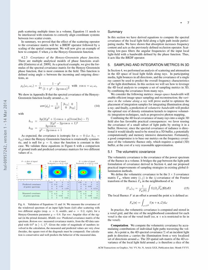
As expected, the covariance is isotropic for α = 0 (i.e. h11 =h22) since the Henyey-Greenstein function is rotationally symmet-ric, and is null for g = 0, since the function is constant in thiscase. We validate these equations in Figure 6 with a comparisonof ground truth and predicted covariance matrices for two differentvalues of α.

Fig. 6. Validation of Equations 11 and 14. We measure the covariance ofthe windowed spectrum of an input light beam (left) after scattering withtwo different angles (resp. α = 0, middle, and α = 0.2, right), for aHenyey-Greentein parameter g = 0.8. Top row: Angular slice of the sig-nal (in the primal domain). Middle row: Predicted covariance matrix of thespectrum. Bottom row: measured covariance matrix, from the 4D data sam-pled with 644 in [−1, 1]4. Given the order of magnitude of numbers in-volved in the calculation, the measured and predicted values are very close(besides, the square root of the diagonals must be compared). Our calcula-tion is conservative and well predicts the behavior of the measured data.

Summary

In this section we have derived equations to compute the spectralcovariance of the local light field along a light path inside partici-pating media. We have shown that absorption increases frequencycontent and acts as the previously defined occlusion operator. Scat-tering low-pass filters the angular frequencies of the input locallight-field with a bandwidth defined by the phase function. Thus,it acts like the BRDF operator.

5. SAMPLING AND INTEGRATION METRICS IN 3D

In Section 4, we performed an analysis of scattering and attenuationin the 4D space of local light fields along rays. In participatingmedia, light bounces in all directions, and the covariance of a singleray cannot be used to predict the overall frequency characteristicsof the light distribution. In this section we will see how to leveragethe 4D local analysis to compute a set of sampling metrics in 3D,by combining the covariance from many rays.

We consider the following metrics: image-space bandwidth willenable efficient image space sampling and reconstruction; the vari-ance in the volume along a ray will prove useful to optimize theplacement of integration samples for integrating illumination alonga ray; and finally, a prediction of volumetric bandwidth will predictthe optimal size of density estimation kernels to improve volumet-ric integration techniques, such as progressive photon mapping,

Combining the 4D local covariance of many rays into a single 3Dfield also has favorable practical consequences: we favor reusingthe covariance of a small subset of light paths by storing it in abuffer. However, since the spectral covariance of radiance is direc-tional it would ideally need to be stored in a 5D buffer, a potentiallycomputationally and memory intensive datastructure. Fortunately,a good compromise is to base our metrics on the frequency covari-ance of the volumetric fluence only, which requires a spatial (3D)buffer, at the cost of a very reasonable approximation.

5.1 The volumetric covariance

The volumetric covariance is the covariance of the power spectrumof the fluence in a volume. It bridges the gap between the light pathformulation of covariance derived in Section 4, and our proposedpractical improvements of sampling strategies in existing global il-lumination methods.

We define the volumetric covariance to be the 3 × 3 covariancematrix Γx, where entry (i, j) is the ij-covariance of the Fouriertransform of the fluence Fx in the neighborhood of x:

(Γx)ij =1

Fx(0)

∫ΩiΩjFx(Ω)dΩ (15)

The local fluence F at an offset s around the point x is defined as:

Fx(s) =

∫ω∈S2

l(x + s, ~ω)dω

In practice, the volumetric covariance is computed and stored ina voxel grid, and the size of the neighborhood considered for eachvoxel is the size of the voxel itself (so, x + s is restricted to lie inthe voxel).

Computation. We compute the volumetric covariance by accu-mulating contributions of individual light paths traversing the vol-ume. At a point x, the 4D spectral covariance Σ of an incident lightpath in direction ω carries the illumination from a very localizedset of directions around ω. The 2D spatial sub-matrix of the 4D co-variance of the local light field around ω is therefore a slice of the


hal-0

0957

242,

ver

sion

1 -

14 M

ar 2

014

8 •

3D covariance of the integrated radiance, in the plane orthogonal toω.

Consequently, we compute the covariance of the fluence at x bysumming up the 2D spatial slices of the covariance matrices of eachincident light path, padded to 3D with zeroes, and rotated to matchthe world coordinate system. Since Σ lives in Fourier space, andthe summation happens in the primal domain, submatrices needto be extracted from Σ−1 and inverted back to Fourier space aftersummation:

Γp =

(∫ω∈S2

RωΣ−1|δx,δyRTω I(ω)dω

)−1

(16)

In this equation, the notation Σ−1|δx,δy refers to the 2D spatial sub-matrix of matrix Σ−1, while Rω is the 3× 2 matrix converting thetwo local spatial coordinates around ω into the three coordinatesof the world. Finally, I(ω) is the normalized incident energy alongincoming direction ω.

In practice, the integral in Equation 16 is computed using a clas-sical Monte Carlo summation, as light paths in the volume crossvoxels they contribute to. We do not need to explicitly computeI(ω) since it is naturally handled by the photon tracing approach:the number of path crossing a voxel is proportional to the fluence.We only record how many times each voxel was hit, for proper nor-malization.

5.2 Image-space covariance

We want to compute image-space covariances for adaptive sam-pling. The angular sub-matrix of the covariance Σ at the cameracan be used to derive sampling densities and reconstruction filtersfor ray-tracing, at each pixel [Belcour et al. 2013].

The most straightforward method to obtain Σ for each pixel inthe screen would be to accumulate covariance matrices from lightpaths reaching the camera, applying the theory of Section 4. Whilethis eventually provides an unbiased estimate of the image-spacecovariance, it needs many light paths to obtain a reasonably noise-free estimate.

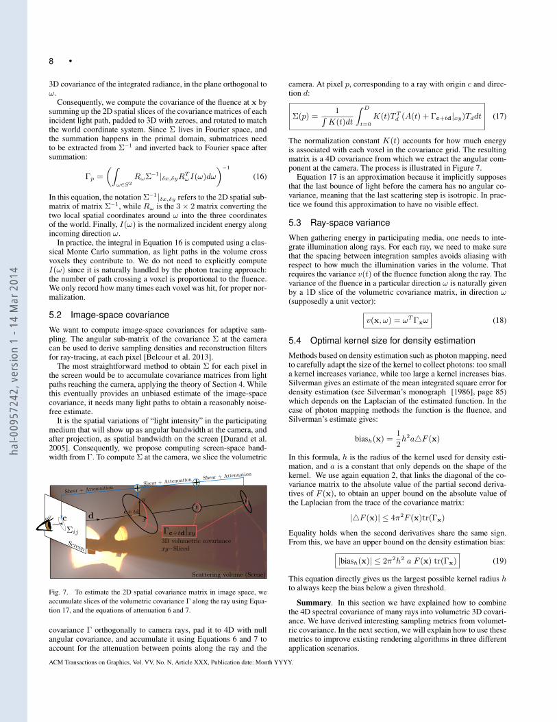
It is the spatial variations of “light intensity” in the participatingmedium that will show up as angular bandwidth at the camera, andafter projection, as spatial bandwidth on the screen [Durand et al.2005]. Consequently, we propose computing screen-space band-width from Γ. To compute Σ at the camera, we slice the volumetric

++

Fig. 7. To estimate the 2D spatial covariance matrix in image space, weaccumulate slices of the volumetric covariance Γ along the ray using Equa-tion 17, and the equations of attenuation 6 and 7.

covariance Γ orthogonally to camera rays, pad it to 4D with nullangular covariance, and accumulate it using Equations 6 and 7 toaccount for the attenuation between points along the ray and the

camera. At pixel p, corresponding to a ray with origin c and direc-tion d:

Σ(p) =1∫

K(t)dt

∫ D

t=0

K(t)TTd (A(t) + Γc+td|xy)Tddt (17)

The normalization constant K(t) accounts for how much energyis associated with each voxel in the covariance grid. The resultingmatrix is a 4D covariance from which we extract the angular com-ponent at the camera. The process is illustrated in Figure 7.

Equation 17 is an approximation because it implicitly supposesthat the last bounce of light before the camera has no angular co-variance, meaning that the last scattering step is isotropic. In prac-tice we found this approximation to have no visible effect.

5.3 Ray-space variance

When gathering energy in participating media, one needs to inte-grate illumination along rays. For each ray, we need to make surethat the spacing between integration samples avoids aliasing withrespect to how much the illumination varies in the volume. Thatrequires the variance v(t) of the fluence function along the ray. Thevariance of the fluence in a particular direction ω is naturally givenby a 1D slice of the volumetric covariance matrix, in direction ω(supposedly a unit vector):

v(x, ω) = ωTΓxω (18)

5.4 Optimal kernel size for density estimation

Methods based on density estimation such as photon mapping, needto carefully adapt the size of the kernel to collect photons: too smalla kernel increases variance, while too large a kernel increases bias.Silverman gives an estimate of the mean integrated square error fordensity estimation (see Silverman’s monograph [1986], page 85)which depends on the Laplacian of the estimated function. In thecase of photon mapping methods the function is the fluence, andSilverman’s estimate gives:

biash(x) =1

2h2a4F (x)

In this formula, h is the radius of the kernel used for density esti-mation, and a is a constant that only depends on the shape of thekernel. We use again equation 2, that links the diagonal of the co-variance matrix to the absolute value of the partial second deriva-tives of F (x), to obtain an upper bound on the absolute value ofthe Laplacian from the trace of the covariance matrix:

|4F (x)| ≤ 4π2F (x)tr(Γx)

Equality holds when the second derivatives share the same sign.From this, we have an upper bound on the density estimation bias:

|biash(x)| ≤ 2π2h2 a F (x) tr(Γx) (19)

This equation directly gives us the largest possible kernel radius hto always keep the bias below a given threshold.

Summary. In this section we have explained how to combinethe 4D spectral covariance of many rays into volumetric 3D covari-ance. We have derived interesting sampling metrics from volumet-ric covariance. In the next section, we will explain how to use thesemetrics to improve existing rendering algorithms in three differentapplication scenarios.


hal-0

0957

242,

ver

sion

1 -

14 M

ar 2

014

• 9

6. IMPROVEMENT OF EXISTING SAMPLING ANDRECONSTRUCTION METHODS

In this section we demonstrate the usefulness of our analysis fromSection 4, and the sampling prediction metrics we derived in Sec-tion 5. We examine four different calculation steps that are involvedin computational methods of global illumination in participatingmedia, and we show that our sampling metrics can be used to ac-celerate them.

Our sampling metrics need the computation of volumetric 3Dcovariance, as defined in Section 5. To compute and store volumet-ric covariance, we use a voxel grid, the covariance grid. In the usecases below, we always read the values of Γ in that grid to computethe required metrics. All results are computed on an Intel i7-3820with four cores at 3.60GHz per core and an NVidia GeForce GTX680. We use 8 threads to benefit from hyperthreading. Unless noted,we use a 643 covariance grid. The covariance grid population algo-rithms run on a single thread, while we use multi-processor capa-bilities for volume integration (Section 6.3 and 6.4 using OpenMP)and for density estimation (Section 6.5 using CUDA).

6.1 The covariance grid

We sample light paths, and populate the covariance grid usingEquation 16. We also record how many times each voxel in the gridis visited by light paths, so as to maintain information for propernormalization.

This calculation is not view-dependent. Depending on the appli-cation, we populate the covariance grid using a fixed proportion ofthe light paths used for the simulation (in Section 6.5), or fill it uponce before the simulation (Sections 6.3 and 6.4). Figure 9 refer-ences the values used for the different scenes. For the algorithmsof Section 6.3 and 6.4, ray marching and filling the covariance gridwith 100, 000 light paths takes 21 seconds for a 643 covariance gridwith the Halloween scene. We used as many as 10, 000 light pathsfor the Sibenik scene, as the lights are spot lights. With this amountof light paths, it took 8 seconds for ray marching and filling for the643 covariance grid.

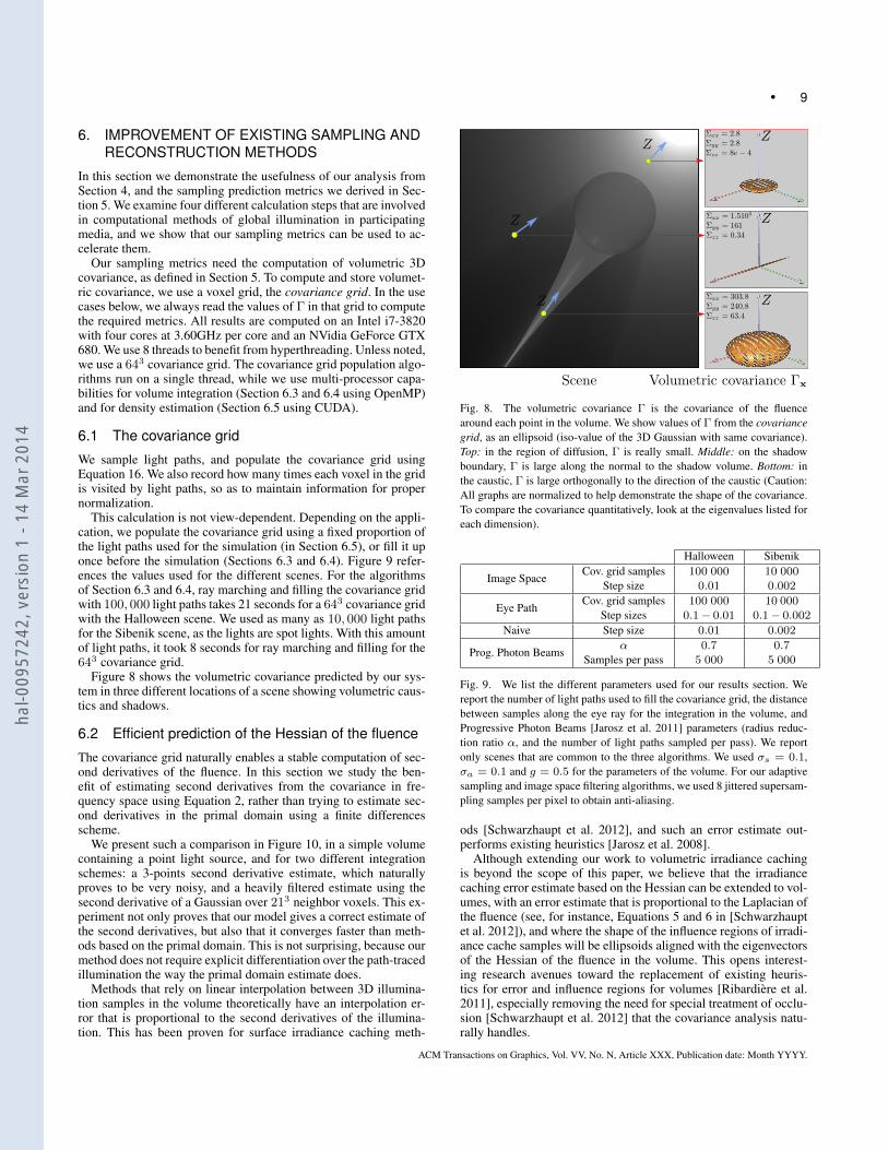
Figure 8 shows the volumetric covariance predicted by our sys-tem in three different locations of a scene showing volumetric caus-tics and shadows.

6.2 Efficient prediction of the Hessian of the fluence

The covariance grid naturally enables a stable computation of sec-ond derivatives of the fluence. In this section we study the ben-efit of estimating second derivatives from the covariance in fre-quency space using Equation 2, rather than trying to estimate sec-ond derivatives in the primal domain using a finite differencesscheme.

We present such a comparison in Figure 10, in a simple volumecontaining a point light source, and for two different integrationschemes: a 3-points second derivative estimate, which naturallyproves to be very noisy, and a heavily filtered estimate using thesecond derivative of a Gaussian over 213 neighbor voxels. This ex-periment not only proves that our model gives a correct estimate ofthe second derivatives, but also that it converges faster than meth-ods based on the primal domain. This is not surprising, because ourmethod does not require explicit differentiation over the path-tracedillumination the way the primal domain estimate does.

Methods that rely on linear interpolation between 3D illumina-tion samples in the volume theoretically have an interpolation er-ror that is proportional to the second derivatives of the illumina-tion. This has been proven for surface irradiance caching meth-

Fig. 8. The volumetric covariance Γ is the covariance of the fluencearound each point in the volume. We show values of Γ from the covariancegrid, as an ellipsoid (iso-value of the 3D Gaussian with same covariance).Top: in the region of diffusion, Γ is really small. Middle: on the shadowboundary, Γ is large along the normal to the shadow volume. Bottom: inthe caustic, Γ is large orthogonally to the direction of the caustic (Caution:All graphs are normalized to help demonstrate the shape of the covariance.To compare the covariance quantitatively, look at the eigenvalues listed foreach dimension).

Halloween Sibenik

Image SpaceCov. grid samples 100 000 10 000

Step size 0.01 0.002

Eye PathCov. grid samples 100 000 10 000

Step sizes 0.1− 0.01 0.1− 0.002

Naive Step size 0.01 0.002

Prog. Photon Beamsα 0.7 0.7

Samples per pass 5 000 5 000

Fig. 9. We list the different parameters used for our results section. Wereport the number of light paths used to fill the covariance grid, the distancebetween samples along the eye ray for the integration in the volume, andProgressive Photon Beams [Jarosz et al. 2011] parameters (radius reduc-tion ratio α, and the number of light paths sampled per pass). We reportonly scenes that are common to the three algorithms. We used σs = 0.1,σa = 0.1 and g = 0.5 for the parameters of the volume. For our adaptivesampling and image space filtering algorithms, we used 8 jittered supersam-pling samples per pixel to obtain anti-aliasing.

ods [Schwarzhaupt et al. 2012], and such an error estimate out-performs existing heuristics [Jarosz et al. 2008].

Although extending our work to volumetric irradiance cachingis beyond the scope of this paper, we believe that the irradiancecaching error estimate based on the Hessian can be extended to vol-umes, with an error estimate that is proportional to the Laplacian ofthe fluence (see, for instance, Equations 5 and 6 in [Schwarzhauptet al. 2012]), and where the shape of the influence regions of irradi-ance cache samples will be ellipsoids aligned with the eigenvectorsof the Hessian of the fluence in the volume. This opens interest-ing research avenues toward the replacement of existing heuris-tics for error and influence regions for volumes [Ribardiere et al.2011], especially removing the need for special treatment of occlu-sion [Schwarzhaupt et al. 2012] that the covariance analysis natu-rally handles.


hal-0

0957

242,

ver

sion

1 -

14 M

ar 2

014

10 •

2

2.5

3

3.5

4

4.5

5

0 10000 20000 30000 40000 50000

Fluence 2nd derivative in primal space (3-points estimate)Fluence 2nd derivative in primal space (21^3-sized filter)Fluence 2nd derivative using 3D covariance (Equation 2)

Total rays cast

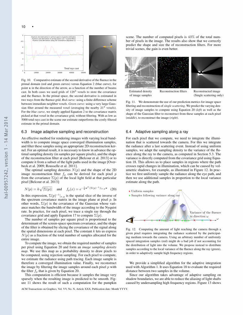
Fig. 10. Comparative estimate of the second derivative of the fluence in theprimal domain (red and green curves) versus Equation 2 (blue curve), forpoint x in the direction of the arrow, as a function of the number of beamscast. In both cases we used grids of 1283 voxels to store the covarianceand the fluence. In the primal space, the second derivative is estimated intwo ways from the fluence grid. Red curve: using a finite difference schemebetween immediate neighbor voxels. Green curve: using a very large Gaus-sian filter around the measured voxel (averaging the nearby 213 voxels).For the blue curve, we simply applied Equation 2 to the covariance matrixpicked at that voxel in the covariance grid, without filtering. With as low as5000 total rays cast in the scene our estimate outperforms the costly filteredestimate in the primal domain.

6.3 Image adaptive sampling and reconstruction

An effective method for rendering images with varying local band-width is to compute image space converged illumination samples,and filter these samples using an appropriate 2D reconstruction ker-nel. For an optimal result, it is necessary to know in advance the op-timal sampling density (in samples per square pixels), and the shapeof the reconstruction filter at each pixel [Belcour et al. 2013] or tocompute it from a subset of the light paths used in the image [Over-beck et al. 2009; Rousselle et al. 2011].

The optimal sampling densities N(p) and the shape of the 2Dimage reconstruction filter fp can be derived for each pixel pfrom the covariance Σ(p) of the local light field at that particularpixel [Belcour et al. 2013]:

N(p) = k√|Σ(p)| and fp(x) = e−

12xT (Σ(p)−1)|x,yx (20)

In this expression, Σ(p)−1|x,y is the spatial slice of the inverse ofthe spectrum covariance matrix in the image plane at pixel p. Inother words, Σ(p) is the covariance of the Gaussian whose vari-ance matches the bandwidth of the image according to the Nyquistrate. In practice, for each pixel, we trace a single ray through thecovariance grid and apply Equation 17 to compute Σ(p).

The number of samples per square pixel is proportional to thedeterminant of the screen-space spectrum covariance, and the shapeof the filter is obtained by slicing the covariance of the signal alongthe spatial dimensions at each pixel. The constant k lets us expressN(p) as a fraction of the total number of samples allocated for theentire image.

To compute the image, we obtain the required number of samplesper pixel using Equation 20 and form an image sampling densitymap. We use this map as a probability density to draw pixels tobe computed, using rejection sampling. For each pixel to compute,we estimate the radiance using path tracing. Each image sample istherefore a converged illumination value. Finally, we reconstructthe image by filtering the image samples around each pixel p withthe filter fp that is given by Equation 20.

This computation is efficient because it samples the image verysparsely when the resulting image is predicted to be smooth. Fig-ure 11 shows the result of such a computation for the pumpkin

scene. The number of computed pixels is 43% of the total num-ber of pixels in the image. The results also show that we correctlypredict the shape and size the of reconstruction filters. For moretrivial scenes, the gain is even better.

Estimated density Reconstruction filters Reconstructed imageof image samples (Single scattering only)

Fig. 11. We demonstrate the use of our prediction metrics for image spacefiltering and reconstruction of single scattering. We predict the varying den-sity of image samples to compute using Equation 20 (left) as well as theshape of the Gaussian filter to reconstruct from these samples at each pixel(middle), to reconstruct the image (right).

6.4 Adaptive sampling along a ray

For each pixel that we compute, we need to integrate the illumi-nation that is scattered towards the camera. For this we integratethe radiance after a last scattering event. Instead of using uniformsamples, we adapt the sampling density to the variance of the flu-ence along the ray to the camera, as computed in Section 5.3. Thevariance is directly computed from the covariance grid using Equa-tion 18. This allows us to place samples in regions where the pathcrosses rapid changes in illumination, which can be caused by vol-umetric shadows, for example, as illustrated in Figure 12. In prac-tice we first uniformly sample the radiance along the eye path, andthen we use additional samples in proportion to the local varianceestimate along the path.

Fig. 12. Computing the amount of light reaching the camera through agiven pixel requires integrating the radiance scattered by the participat-ing medium towards the camera. Using an arbitrary number of uniformlyspaced integration samples (red) might do a bad job if not accounting forthe distribution of light into the volume. We propose instead to distributesamples according to the local variance of the fluence along the ray (green),in order to adaptively sample high frequency regions.

We provide a simplified algorithm for the adaptive integrationused with Algorithm 1. It uses Equation 18 to evaluate the requireddistance between two samples in the volume.

Since our algorithm takes advantage of adaptive sampling onshadow boundaries, we are able to reduce the aliasing of light shaftscaused by undersampling high frequency regions. Figure 13 shows


hal-0

0957

242,

ver

sion

1 -

14 M

ar 2

014

• 11

Algorithm 1 Our adaptive sampling algorithm compute the singlescattering radiance for an eye ray defined by its position x in spaceand direction ω. It returns the light scattered by the volume in theinterval [0, Tmax] along the ray. Our variance estimate v (Equa-tion 18) provides a step size in the volume. Note that the last steprequires special treatment as the step might be larger than the re-maining integration distance. We do not show it in this example tokeep a compact formulation.

function ADAPTIVEINTEGRATION(x, ω, Tmax, stepmin,stepmax)

rad = 0t = 0while t ∈ [0..Tmax] do

xt = x + tω

dt =1

2√v(xt, ω)

dt = clamp(dt, stepmin, stepmax)rad = rad+ dt integrateRadiance(xt,−ω)t = t+ dt

end whilereturn rad

end function

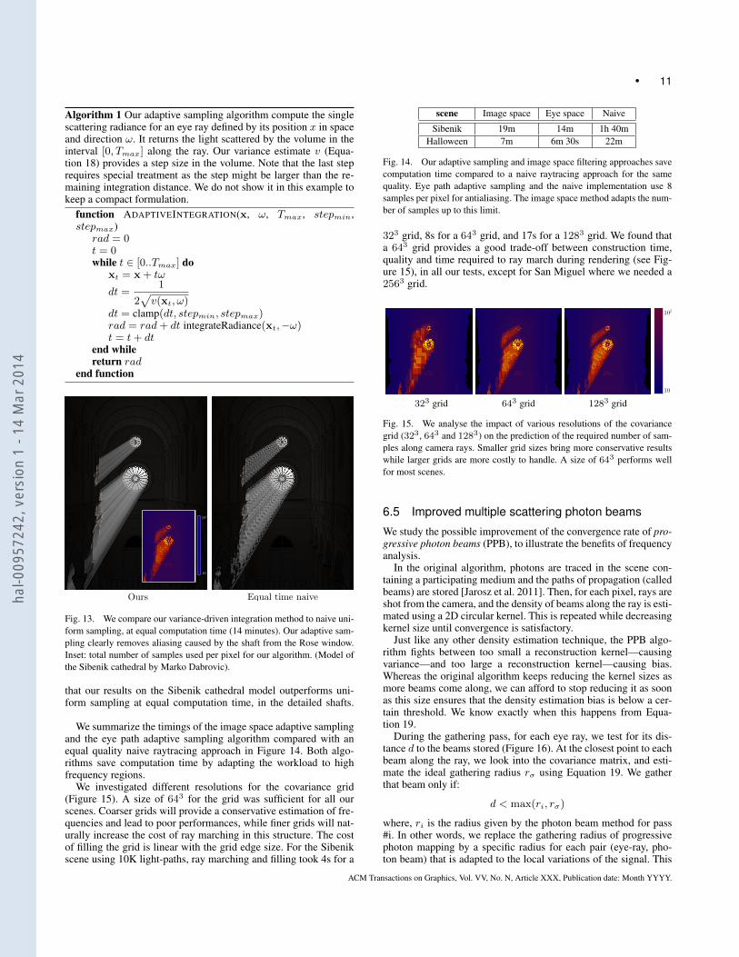
Fig. 13. We compare our variance-driven integration method to naive uni-form sampling, at equal computation time (14 minutes). Our adaptive sam-pling clearly removes aliasing caused by the shaft from the Rose window.Inset: total number of samples used per pixel for our algorithm. (Model ofthe Sibenik cathedral by Marko Dabrovic).

that our results on the Sibenik cathedral model outperforms uni-form sampling at equal computation time, in the detailed shafts.

We summarize the timings of the image space adaptive samplingand the eye path adaptive sampling algorithm compared with anequal quality naive raytracing approach in Figure 14. Both algo-rithms save computation time by adapting the workload to highfrequency regions.

We investigated different resolutions for the covariance grid(Figure 15). A size of 643 for the grid was sufficient for all ourscenes. Coarser grids will provide a conservative estimation of fre-quencies and lead to poor performances, while finer grids will nat-urally increase the cost of ray marching in this structure. The costof filling the grid is linear with the grid edge size. For the Sibenikscene using 10K light-paths, ray marching and filling took 4s for a

scene Image space Eye space Naive

Sibenik 19m 14m 1h 40mHalloween 7m 6m 30s 22m

Fig. 14. Our adaptive sampling and image space filtering approaches savecomputation time compared to a naive raytracing approach for the samequality. Eye path adaptive sampling and the naive implementation use 8samples per pixel for antialiasing. The image space method adapts the num-ber of samples up to this limit.

323 grid, 8s for a 643 grid, and 17s for a 1283 grid. We found thata 643 grid provides a good trade-off between construction time,quality and time required to ray march during rendering (see Fig-ure 15), in all our tests, except for San Miguel where we needed a2563 grid.

323 grid 643 grid 1283 grid

Fig. 15. We analyse the impact of various resolutions of the covariancegrid (323, 643 and 1283) on the prediction of the required number of sam-ples along camera rays. Smaller grid sizes bring more conservative resultswhile larger grids are more costly to handle. A size of 643 performs wellfor most scenes.

6.5 Improved multiple scattering photon beams

We study the possible improvement of the convergence rate of pro-gressive photon beams (PPB), to illustrate the benefits of frequencyanalysis.

In the original algorithm, photons are traced in the scene con-taining a participating medium and the paths of propagation (calledbeams) are stored [Jarosz et al. 2011]. Then, for each pixel, rays areshot from the camera, and the density of beams along the ray is esti-mated using a 2D circular kernel. This is repeated while decreasingkernel size until convergence is satisfactory.

Just like any other density estimation technique, the PPB algo-rithm fights between too small a reconstruction kernel—causingvariance—and too large a reconstruction kernel—causing bias.Whereas the original algorithm keeps reducing the kernel sizes asmore beams come along, we can afford to stop reducing it as soonas this size ensures that the density estimation bias is below a cer-tain threshold. We know exactly when this happens from Equa-tion 19.

During the gathering pass, for each eye ray, we test for its dis-tance d to the beams stored (Figure 16). At the closest point to eachbeam along the ray, we look into the covariance matrix, and esti-mate the ideal gathering radius rσ using Equation 19. We gatherthat beam only if:

d < max(ri, rσ)

where, ri is the radius given by the photon beam method for pass#i. In other words, we replace the gathering radius of progressivephoton mapping by a specific radius for each pair (eye-ray, pho-ton beam) that is adapted to the local variations of the signal. This


hal-0

0957

242,

ver

sion

1 -

14 M

ar 2

014

12 •

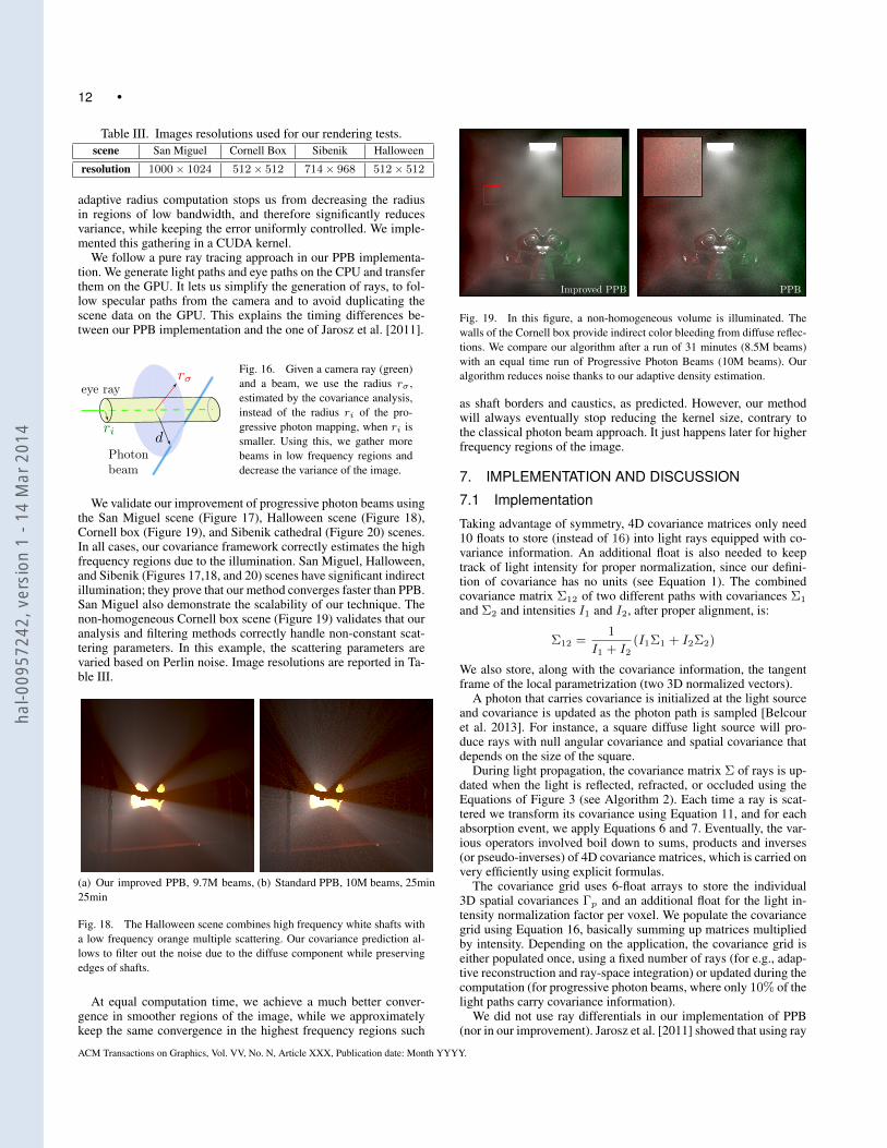
Table III. Images resolutions used for our rendering tests.scene San Miguel Cornell Box Sibenik Halloween

resolution 1000× 1024 512× 512 714× 968 512× 512

adaptive radius computation stops us from decreasing the radiusin regions of low bandwidth, and therefore significantly reducesvariance, while keeping the error uniformly controlled. We imple-mented this gathering in a CUDA kernel.

We follow a pure ray tracing approach in our PPB implementa-tion. We generate light paths and eye paths on the CPU and transferthem on the GPU. It lets us simplify the generation of rays, to fol-low specular paths from the camera and to avoid duplicating thescene data on the GPU. This explains the timing differences be-tween our PPB implementation and the one of Jarosz et al. [2011].

Fig. 16. Given a camera ray (green)and a beam, we use the radius rσ ,estimated by the covariance analysis,instead of the radius ri of the pro-gressive photon mapping, when ri issmaller. Using this, we gather morebeams in low frequency regions anddecrease the variance of the image.

We validate our improvement of progressive photon beams usingthe San Miguel scene (Figure 17), Halloween scene (Figure 18),Cornell box (Figure 19), and Sibenik cathedral (Figure 20) scenes.In all cases, our covariance framework correctly estimates the highfrequency regions due to the illumination. San Miguel, Halloween,and Sibenik (Figures 17,18, and 20) scenes have significant indirectillumination; they prove that our method converges faster than PPB.San Miguel also demonstrate the scalability of our technique. Thenon-homogeneous Cornell box scene (Figure 19) validates that ouranalysis and filtering methods correctly handle non-constant scat-tering parameters. In this example, the scattering parameters arevaried based on Perlin noise. Image resolutions are reported in Ta-ble III.

(a) Our improved PPB, 9.7M beams,25min

(b) Standard PPB, 10M beams, 25min

Fig. 18. The Halloween scene combines high frequency white shafts witha low frequency orange multiple scattering. Our covariance prediction al-lows to filter out the noise due to the diffuse component while preservingedges of shafts.

At equal computation time, we achieve a much better conver-gence in smoother regions of the image, while we approximatelykeep the same convergence in the highest frequency regions such

Fig. 19. In this figure, a non-homogeneous volume is illuminated. Thewalls of the Cornell box provide indirect color bleeding from diffuse reflec-tions. We compare our algorithm after a run of 31 minutes (8.5M beams)with an equal time run of Progressive Photon Beams (10M beams). Ouralgorithm reduces noise thanks to our adaptive density estimation.

as shaft borders and caustics, as predicted. However, our methodwill always eventually stop reducing the kernel size, contrary tothe classical photon beam approach. It just happens later for higherfrequency regions of the image.

7. IMPLEMENTATION AND DISCUSSION

7.1 Implementation

Taking advantage of symmetry, 4D covariance matrices only need10 floats to store (instead of 16) into light rays equipped with co-variance information. An additional float is also needed to keeptrack of light intensity for proper normalization, since our defini-tion of covariance has no units (see Equation 1). The combinedcovariance matrix Σ12 of two different paths with covariances Σ1

and Σ2 and intensities I1 and I2, after proper alignment, is:

Σ12 =1

I1 + I2(I1Σ1 + I2Σ2)

We also store, along with the covariance information, the tangentframe of the local parametrization (two 3D normalized vectors).

A photon that carries covariance is initialized at the light sourceand covariance is updated as the photon path is sampled [Belcouret al. 2013]. For instance, a square diffuse light source will pro-duce rays with null angular covariance and spatial covariance thatdepends on the size of the square.

During light propagation, the covariance matrix Σ of rays is up-dated when the light is reflected, refracted, or occluded using theEquations of Figure 3 (see Algorithm 2). Each time a ray is scat-tered we transform its covariance using Equation 11, and for eachabsorption event, we apply Equations 6 and 7. Eventually, the var-ious operators involved boil down to sums, products and inverses(or pseudo-inverses) of 4D covariance matrices, which is carried onvery efficiently using explicit formulas.

The covariance grid uses 6-float arrays to store the individual3D spatial covariances Γp and an additional float for the light in-tensity normalization factor per voxel. We populate the covariancegrid using Equation 16, basically summing up matrices multipliedby intensity. Depending on the application, the covariance grid iseither populated once, using a fixed number of rays (for e.g., adap-tive reconstruction and ray-space integration) or updated during thecomputation (for progressive photon beams, where only 10% of thelight paths carry covariance information).

We did not use ray differentials in our implementation of PPB(nor in our improvement). Jarosz et al. [2011] showed that using ray


hal-0

0957

242,

ver

sion

1 -

14 M

ar 2

014

• 13

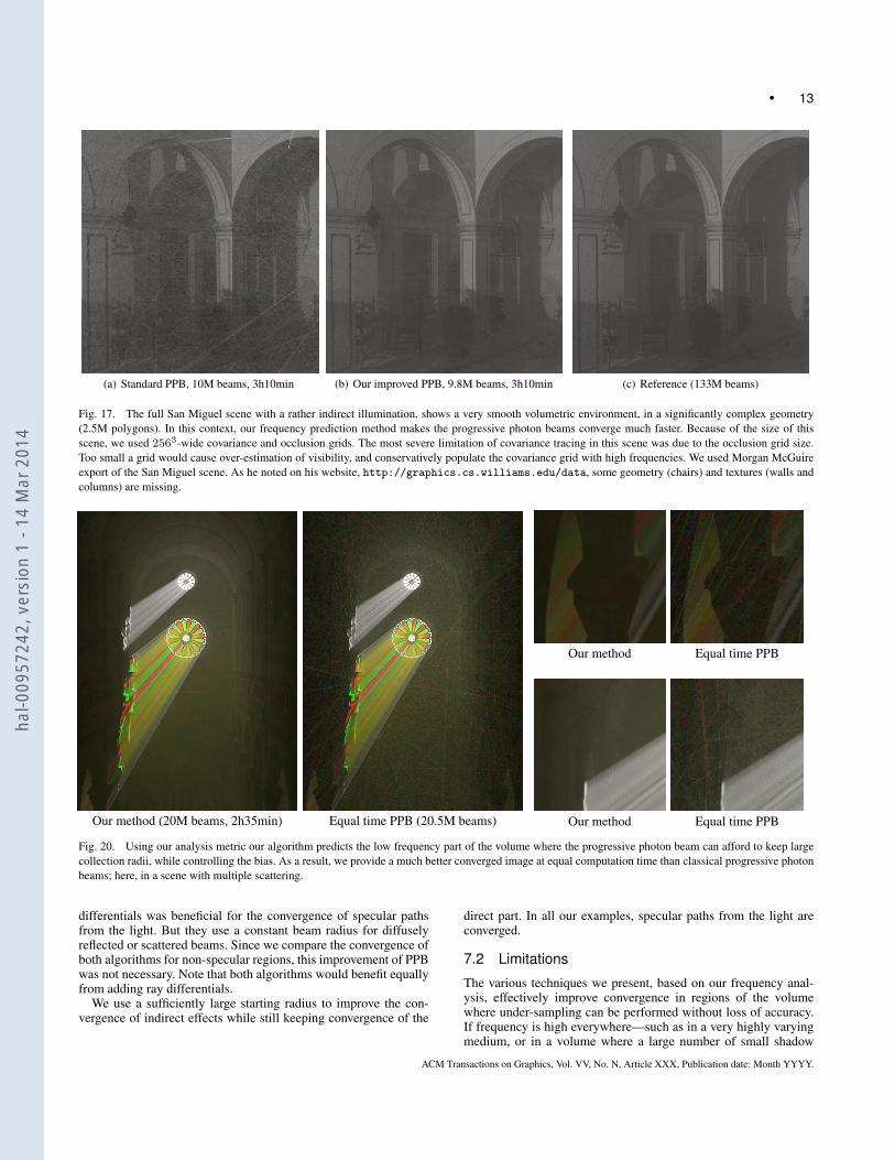
(a) Standard PPB, 10M beams, 3h10min (b) Our improved PPB, 9.8M beams, 3h10min (c) Reference (133M beams)

Fig. 17. The full San Miguel scene with a rather indirect illumination, shows a very smooth volumetric environment, in a significantly complex geometry(2.5M polygons). In this context, our frequency prediction method makes the progressive photon beams converge much faster. Because of the size of thisscene, we used 2563-wide covariance and occlusion grids. The most severe limitation of covariance tracing in this scene was due to the occlusion grid size.Too small a grid would cause over-estimation of visibility, and conservatively populate the covariance grid with high frequencies. We used Morgan McGuireexport of the San Miguel scene. As he noted on his website, http://graphics.cs.williams.edu/data, some geometry (chairs) and textures (walls andcolumns) are missing.

Our method (20M beams, 2h35min) Equal time PPB (20.5M beams)

Our method Equal time PPB

Our method Equal time PPB

Fig. 20. Using our analysis metric our algorithm predicts the low frequency part of the volume where the progressive photon beam can afford to keep largecollection radii, while controlling the bias. As a result, we provide a much better converged image at equal computation time than classical progressive photonbeams; here, in a scene with multiple scattering.

differentials was beneficial for the convergence of specular pathsfrom the light. But they use a constant beam radius for diffuselyreflected or scattered beams. Since we compare the convergence ofboth algorithms for non-specular regions, this improvement of PPBwas not necessary. Note that both algorithms would benefit equallyfrom adding ray differentials.

We use a sufficiently large starting radius to improve the con-vergence of indirect effects while still keeping convergence of the

direct part. In all our examples, specular paths from the light areconverged.

7.2 Limitations

The various techniques we present, based on our frequency anal-ysis, effectively improve convergence in regions of the volumewhere under-sampling can be performed without loss of accuracy.If frequency is high everywhere—such as in a very highly varyingmedium, or in a volume where a large number of small shadow


hal-0

0957

242,

ver

sion

1 -

14 M

ar 2

014

14 •

Algorithm 2 The tracing of frequency photons is straightforwardto implement. It only requires that we update the covariance ma-trix at specific steps. Note that it requires the ray tracing engine tocompute specific information for intersection with geometry (suchas local curvature). TheRmatrix is the factorized matrix of projec-tion, alignment and curvature, before and after reflection. T is thecovariance of the texture matrix.

function TRACEFREQUENCYPHOTONp, ω ← sampleLight()Σ← computeLightCovariance()while russianRoulette() do

p← traceRay(p, ω)for all voxels v until hit do

updateVoxelCovariance(v,Σ)Σ← TTd ΣTdΣ← Σ +OΣ← Σ +A

end forω ← sampleBRDF()Σ← RTi ΣRiΣ← Σ + TΣ← RTo

(Σ−1 +B

)−1Ro

end whileend function

rays are cast—our a priori analysis naturally predicts that the sam-pling needs to be uniformly dense. In this case, the computation ofcovariance information would naturally not help improve conver-gence.

Using volumetric covariance implies an approximation, since itneglects the angular covariance of the incident light. Our methodcaptures variations in the volumetric fluence which, for reasonablynon-specular phase functions, remains close to the variance of theradiance, while only requiring a small storage cost. In the case ofa very specular phase function at the last bounce before the cam-era, a 3D covariance grid is likely to produce a conservative over-estimation of the bandwidth. A more accurate approach would re-quire also storing directional information into the covariance grid,and does not invalidate our frequency analysis.

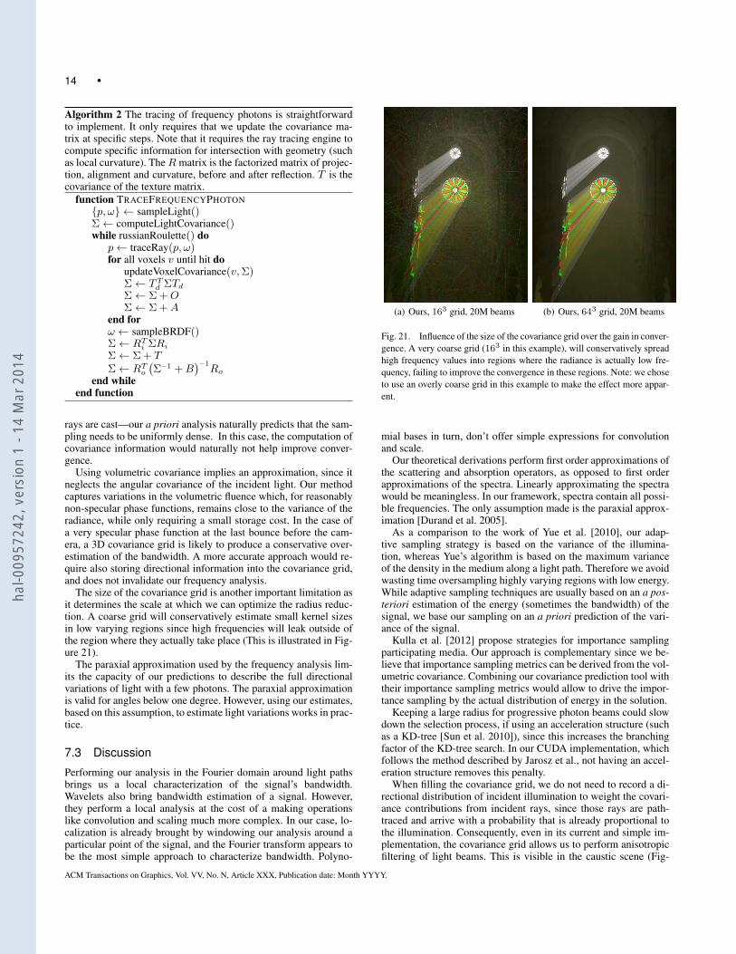
The size of the covariance grid is another important limitation asit determines the scale at which we can optimize the radius reduc-tion. A coarse grid will conservatively estimate small kernel sizesin low varying regions since high frequencies will leak outside ofthe region where they actually take place (This is illustrated in Fig-ure 21).

The paraxial approximation used by the frequency analysis lim-its the capacity of our predictions to describe the full directionalvariations of light with a few photons. The paraxial approximationis valid for angles below one degree. However, using our estimates,based on this assumption, to estimate light variations works in prac-tice.

7.3 Discussion

Performing our analysis in the Fourier domain around light pathsbrings us a local characterization of the signal’s bandwidth.Wavelets also bring bandwidth estimation of a signal. However,they perform a local analysis at the cost of a making operationslike convolution and scaling much more complex. In our case, lo-calization is already brought by windowing our analysis around aparticular point of the signal, and the Fourier transform appears tobe the most simple approach to characterize bandwidth. Polyno-

(a) Ours, 163 grid, 20M beams (b) Ours, 643 grid, 20M beams

Fig. 21. Influence of the size of the covariance grid over the gain in conver-gence. A very coarse grid (163 in this example), will conservatively spreadhigh frequency values into regions where the radiance is actually low fre-quency, failing to improve the convergence in these regions. Note: we choseto use an overly coarse grid in this example to make the effect more appar-ent.

mial bases in turn, don’t offer simple expressions for convolutionand scale.

Our theoretical derivations perform first order approximations ofthe scattering and absorption operators, as opposed to first orderapproximations of the spectra. Linearly approximating the spectrawould be meaningless. In our framework, spectra contain all possi-ble frequencies. The only assumption made is the paraxial approx-imation [Durand et al. 2005].

As a comparison to the work of Yue et al. [2010], our adap-tive sampling strategy is based on the variance of the illumina-tion, whereas Yue’s algorithm is based on the maximum varianceof the density in the medium along a light path. Therefore we avoidwasting time oversampling highly varying regions with low energy.While adaptive sampling techniques are usually based on an a pos-teriori estimation of the energy (sometimes the bandwidth) of thesignal, we base our sampling on an a priori prediction of the vari-ance of the signal.

Kulla et al. [2012] propose strategies for importance samplingparticipating media. Our approach is complementary since we be-lieve that importance sampling metrics can be derived from the vol-umetric covariance. Combining our covariance prediction tool withtheir importance sampling metrics would allow to drive the impor-tance sampling by the actual distribution of energy in the solution.

Keeping a large radius for progressive photon beams could slowdown the selection process, if using an acceleration structure (suchas a KD-tree [Sun et al. 2010]), since this increases the branchingfactor of the KD-tree search. In our CUDA implementation, whichfollows the method described by Jarosz et al., not having an accel-eration structure removes this penalty.

When filling the covariance grid, we do not need to record a di-rectional distribution of incident illumination to weight the covari-ance contributions from incident rays, since those rays are path-traced and arrive with a probability that is already proportional tothe illumination. Consequently, even in its current and simple im-plementation, the covariance grid allows us to perform anisotropicfiltering of light beams. This is visible in the caustic scene (Fig-


hal-0

0957

242,

ver

sion

1 -

14 M

ar 2

014

• 15

ure 8) where we can see that the covariance estimates capture thedirectional discontinuities of the light distribution.

We chose to apply our framework to accelerate progressive pho-ton beams rather than the more recent progressive virtual beamlights [Novak et al. 2012]. The two methods, however, use a similariterative radius reduction scheme. Therefore, one can expect to im-prove on the latter the same way we improve on progressive photonbeams, using our radius reduction stopping criterion.

Similar to Novak et al. [2012], we could use our method to onlyreconstruct the multiple scattering component of the illuminationand not store the specular contribution into the covariance grid. Al-though did not do that, we still produce convincing results as ourmethod adapts to any effect (be it direct of indirect). Treating in-direct scattering independently would enhance the speedup factorof our method as the reconstructed signal would be of even lowerfrequency. But this would increase the required engineering for theimplementation (multiple photon maps would be required).

Our improved progressive photon beams method removes theneed to finely tune the parameters of the radius reduction. This,in a way, is similar to the Adaptive Progressive Photon Mapping ofKaplanyan and Daschbacher [2013]. One notable difference is thatour method does not need to evaluate the Hessian of the radianceusing density estimation, and as shown in Section 6.2 our estimateis much more robust.

Adding the time analysis [Belcour et al. 2013] is straightforwardbut currently limited to rigid motion. The analysis of time varyingmedia is also possible, but beyond the scope of this paper. Timeanalysis could be implemented using the 3D covariance grid by in-tegrating the time dimension. This way, motion events are blurredaccording to the resulting appearance. A 4D grid would be neces-sary to perform temporal coherent filtering. Adding depth of fieldis also orthogonal to this work, but we expect it would not causeparticular issues.

8. CONCLUSION

We proposed the first extension to participating media, of theFourier analysis of local light fields. This is a very important prob-lem that is amenable to performance acceleration, since participat-ing media typically has lower frequencies.

We show how to extend the use of covariance matrices in a prin-cipled manner to represent the spectrum of the light field includingscattering and absorption. We derive the equations to combine theinformation carried by each light path into a set of 3D frequencyprediction metrics, and to compute them from a common quantity:the volumetric covariance, stored in a grid. We used these metricsto improve the convergence and efficiency of image-space adaptivesampling and reconstruction, camera ray integration, and for accel-erating the progressive photon beam approach.

Several future avenues of research exist. While we demonstratedthe use of this analysis for the gather part of photon mapping, ourfrequency estimate could also be used to drive photon tracing, like,for example, using a function of frequency as the acceptance func-tion of Metropolis photon sampling [Fan et al. 2005]. Another inter-esting research avenue would be to extend our analysis to orientedmedia [Jakob et al. 2010].

We did not use an adaptive covariance grid. To do that, the localresolution of the covariance grid needs to be adapted to the varia-tions of the covariance information to be stored, and would sparethe need to specify an initial resolution. We leave this question tofuture work.

ACKNOWLEDGMENTSThe authors thank user Mundomupa from blendswap.com for thedesign of the pumpkin model (used in the Halloween scene) andJeremy Birn for the design of the house front (used in the Hal-loween scene).

The authors also thank Romain Pacanowski for this helpful com-ments during the redaction of this work.

This work was supported in part by a grant ANR-11-BS02-006”ALTA”.

REFERENCES

BAGHER, M., SOLER, C., SUBR, K., BELCOUR, L., AND HOLZSCHUCH,N. 2012. Interactive rendering of acquired materials on dynamic ge-ometry using bandwidth prediction. In Proceedings of the 2012 ACMSiggraph Symposium on Interactive 3D Graphics and Games - I3D. 127–134.

BARAN, I., CHEN, J., RAGAN-KELLEY, J., DURAND, F., AND LEHTI-NEN, J. 2010. A hierarchical volumetric shadow algorithm for singlescattering. ACM Transactions on Graphics (Proceedings of ACM SIG-GRAPH Asia 2010) 29, 6 (Dec.), 178:1–178:10.

BELCOUR, L. AND SOLER, C. 2011. Frequency based kernel estima-tion for progressive photon mapping. In SIGGRAPH Asia 2011 Posters.ACM, 1.

BELCOUR, L., SOLER, C., SUBR, K., HOLZSCHUCH, N., AND DURAND,F. 2013. 5D Covariance Tracing for Efficient Defocus and Motion Blur.ACM Transactions on Graphics 32, 3 (July), 31:1–31:18.

CEREZO, E., PEREZ-CAZORLA, F., PUEYO, X., SERON, F., AND SIL-LION, F. X. 2005. A survey on participating media rendering techniques.The Visual Computer 21, 5 (June), 303–328.

CHEN, J., BARAN, I., DURAND, F., AND JAROSZ, W. 2011. Real-timevolumetric shadows using 1D min-max mipmaps. In Symposium on In-teractive 3D Graphics and Games on - I3D 2011. ACM, 39–46.

DAVE, J. V. 1970. Coefficients of the Legendre and Fourier series for thescattering functions of spherical particles. Applied Optics 9, 8, 1888–1896.

DAVE, J. V. AND GAZDAG, J. 1970. A modified Fourier transform methodfor multiple scattering calculations in a plane parallel Mie atmosphere.Applied Optics 9, 6, 1457–1466.

DUDERSTADT, J. AND MARTIN, W. 1979. Transport Theory. Wiley-Interscience Publications. Wiley.

DURAND, F., HOLZSCHUCH, N., SOLER, C., CHAN, E., AND SILLION,F. X. 2005. A frequency analysis of light transport. ACM TransactionsGraphics (Proceedings of ACM SIGGRAPH 2005) 24, 3 (July), 1115–1126.

EGAN, K., DURAND, F., AND RAMAMOORTHI, R. 2011. Practical fil-tering for efficient ray-traced directional occlusion. ACM Transactionson Graphics (Proceedings of ACM SIGGRAPH Asia 2011) 30, 6 (Dec.),180:1–180:10.

EGAN, K., HECHT, F., DURAND, F., AND RAMAMOORTHI, R. 2011. Fre-quency analysis and sheared filtering for shadow light fields of complexoccluders. ACM Transactions on Graphics 30, 2 (Apr.), 1–13.

EGAN, K., TSENG, Y.-T., HOLZSCHUCH, N., DURAND, F., AND RA-MAMOORTHI, R. 2009. Frequency analysis and sheared reconstructionfor rendering motion blur. ACM Transactions on Graphics (Proceedingsof ACM SIGGRAPH 2009) 28, 3, 93:1–93:13.

ENGELHARDT, T. AND DACHSBACHER, C. 2010. Epipolar sampling forshadows and crepuscular rays in participating media with single scatter-ing. In Proceedings of the 2010 ACM SIGGRAPH Symposium on Inter-active 3D Graphics and Games - I3D. 119–125.


hal-0

0957

242,

ver

sion

1 -

14 M

ar 2

014

16 •

ENGELHARDT, T., NOVAK, J., AND DACHSBACHER, C. 2010. InstantMultiple Scattering for Interactive Rendering of Heterogeneous Partici-pating Media. Tech. rep., Karlsruhe Institut of Technology.

FAN, S., CHENNEY, S., AND CHI LAI, Y. 2005. Metropolis photon sam-pling with optional user guidance. In Proceedings of the 16th Eurograph-ics Symposium on Rendering Techniques 2005. Eurographics Associa-tion, 127–138.

GIRAUD, B. AND PESCHANSKI, R. 2006. On positive functions with pos-itive Fourier transforms. Acta Physica Polonica B 37, 2 (February), 331–343.

GORTLER, S. J., GRZESZCZUK, R., SZELISKI, R., AND COHEN, M. 1986.The Lumigraph. In Proceedings of ACM SIGGRAPH 1996. ACM, 43–54.

GUTIERREZ, D., JENSEN, H. W., JAROSZ, W., AND DONNER, C. 2009.Scattering. In ACM SIGGRAPH Asia 2009 Courses. 15:1–15:620.

IGEHY, H. 1999. Tracing ray differentials. In Proceedings of ACM SIG-GRAPH 1999. ACM, 179–186.

IHRKE, I., ZIEGLER, G., TEVS, A., THEOBALT, C., MAGNOR, M., AND

SEIDEL, H.-P. 2007. Eikonal rendering: efficient light transport in re-fractive objects. 26, 3 (July).

ISHIMARU, A. 1997. Wave Propagation and Scattering in Random Media.IEEE Press and Oxford University Press.

JAKOB, W., ARBREE, A., MOON, J. T., BALA, K., AND MARSCHNER,S. 2010. A radiative transfer framework for rendering materials withanisotropic structure. ACM Transactions on Graphics (Proceedings ofACM SIGGRAPH 2010) 29, 4 (July), 53:1–53:13.

JAROSZ, W., DONNER, C., ZWICKER, M., AND JENSEN, H. W. 2008.Radiance caching for participating media. ACM Transactions on Graph-ics 27, 1 (Mar.), 7:1–7:11.

JAROSZ, W., NOWROUZEZAHRAI, D., SADEGHI, I., AND JENSEN, H. W.2011. A comprehensive theory of volumetric radiance estimation usingphoton points and beams. ACM Transactions on Graphics 30, 1 (Feb.),5:1–5:19.

JAROSZ, W., NOWROUZEZAHRAI, D., THOMAS, R., SLOAN, P.-P., AND

ZWICKER, M. 2011. Progressive photon beams. ACM Transactionson Graphics (Proceedings of ACM SIGGRAPH Asia 2011) 30, 6 (Dec.),181:1–181:12.

JAROSZ, W., ZWICKER, M., AND JENSEN, H. W. 2008. The beam radi-ance estimate for volumetric photon mapping. Computer Graphics Fo-rum 27, 2 (Apr.), 557–566.

JENSEN, H. W. AND CHRISTENSEN, P. H. 1998. Efficient simulation oflight transport in scences with participating media using photon maps. InProceedings of ACM SIGGRAPH 1998. 311–320.

KAJIYA, J. T. AND VON HERZEN, B. P. 1984. Ray tracing volumedensities. ACM Computer Graphics (Proceedings of ACM SIGGRAPH1984) 18, 3 (July), 165–174.

KAPLANYAN, A. S. AND DACHSBACHER, C. 2013. Adaptive progressivephoton mapping. ACM Transactions on Graphics 32, 2 (Apr.), 16:1–16:13.

KIM, A. D. AND MOSCOSO, M. 2003. Radiative transfer computations foroptical beams. Journal Computational Physics 185, 1 (Feb.), 50–60.

KNAUS, C. AND ZWICKER, M. 2011. Progressive photon mapping: Aprobabilistic approach. ACM Transactions on Graphics 30, 3 (May),25:1–25:13.

KULLA, C. AND FAJARDO, M. 2012. Importance sampling techniques forpath tracing in participating media. Computer Graphics Forum (Proceed-ings of EGSR 2012) 31, 4 (June), 1519–1528.

LAFORTUNE, E. P. AND WILLEMS, Y. D. 1993. Bi-directional path trac-ing. In Proceedings of third international conference on computationalgraphics and visualization techniques. 145–153.

LAFORTUNE, E. P. AND WILLEMS, Y. D. 1996. Rendering participatingmedia with bidirectional path tracing. In Proceedings of the EurographicsWorkshop on Rendering Techniques. Springer-Verlag, 91–100.

LEHTINEN, J., AILA, T., CHEN, J., LAINE, S., AND DURAND, F.2011. Temporal light field reconstruction for rendering distribution ef-fects. ACM Transactions on Graphics (Proceedings of ACM SIGGRAPH2011) 30, 4 (July), 55:1–55:12.

LEVOY, M. AND HANRAHAN, P. 1986. Light field rendering. In Proceed-ings of ACM SIGGRAPH 1996. ACM, 31–42.

MEHTA, S., WANG, B., AND RAMAMOORTHI, R. 2012. Axis-aligned fil-tering for interactive sampled soft shadows (proceedings of acm siggraphasia 2012). ACM Transactions on Graphics 31, 6 (Nov), 163:1–163:10.

NOVAK, J., NOWROUZEZAHRAI, D., DACHSBACHER, C., AND JAROSZ,W. 2012. Progressive virtual beam lights. Computer Graphics Forum(Proceedings of EGSR 2012) 31, 4 (June), 1407–1413.

NOVAK, J., NOWROUZEZAHRAI, D., DACHSBACHER, C., AND JAROSZ,W. 2012. Virtual ray lights for rendering scenes with participating me-dia (proceedings of acm siggraph 2012). ACM Transactions on Graph-ics 31, 4 (July), 60:1–60:11.

OVERBECK, R. S., DONNER, C., AND RAMAMOORTHI, R. 2009. Adap-tive wavelet rendering. In ACM Transactions on Graphics (Proceedingsof ACM SIGGRAPH Asia 2009). Vol. 28. 140:1–140:12.

PAULY, M., KOLLIG, T., AND KELLER, A. 2000. Metropolis Light Trans-port for Participating Media. Proceedings of the Eurographics Workshopon Rendering Techniques.

RAMAMOORTHI, R., ANDERSON, J., MEYER, M., AND

NOWROUZEZAHRAI, D. 2012. A theory of monte carlo visibilitysampling. ACM Transactions on Graphics 31, 5 (Sept.), 121:1–121:16.

RIBARDIERE, M., CARRE, S., AND BOUATOUCH, K. 2011. Adaptiverecords for volume irradiance caching. The Visual Computer 27, 6-8(Apr.), 655–664.

RITCHIE, B., DYKEMA, P. G., AND BRADDY, D. 1997. Use of fast-Fourier-transform computational methods in radiation transport. PhysicalReiew E 56, 2 (Aug), 2217–2227.

ROUSSELLE, F., KNAUS, C., AND ZWICKER, M. 2011. Adaptive samplingand reconstruction using greedy error minimization. ACM Transactionson Graphics (Proceedings of ACM SIGGRAPH Asia 2011) 30, 6 (Dec.),159:1–159:12.

RYBICKI, G. B. 1971. The searchlight problem with isotropic scattering.Journal of Quantitative Spectroscopy and Radiative Transfer 11, 6.

SCHWARZHAUPT, J., JENSEN, H. W., AND JAROSZ, W. 2012. Practicalhessian-based error control for irradiance caching. ACM Transactionson Graphics (Proceedings of ACM SIGGRAPH Asia 2012) 31, 6 (Nov.),193:1–193:10.

SILVERMAN, B. 1986. Density Estimation for Statistics and Data Analysis,1 ed. Chapman and Hall/CRC.

SOLER, C., SUBR, K., DURAND, F., HOLZSCHUCH, N., AND SILLION,F. X. 2009. Fourier depth of field. ACM Transactions on Graphics 28, 2,18:1–18:12.

SUN, X., ZHOU, K., LIN, S., AND GUO, B. 2010. Line space gather-ing for single scattering in large scenes. ACM Transactions on Graphics(Proceedings of ACM SIGGRAPH 2010) 29, 4 (July), 54:1–54:8.

TODHUNTER, I. 1859. Spherical Trigonometry, for the use of Colleges andSchools. Macmillan and Company.

VEACH, E. AND GUIBAS, L. J. 1997. Metropolis light transport. In Pro-ceedings of ACM SIGGRAPH 1997. ACM, 65–76.

WALTER, B., ARBREE, A., BALA, K., AND GREENBERG, D. P. 2006.Multidimensional lightcuts. ACM Transactions on Graphics (Proceed-ings of ACM SIGGRAPH 2006) 25, 3 (July), 1081–1088.


hal-0

0957

242,

ver

sion

1 -

14 M

ar 2

014

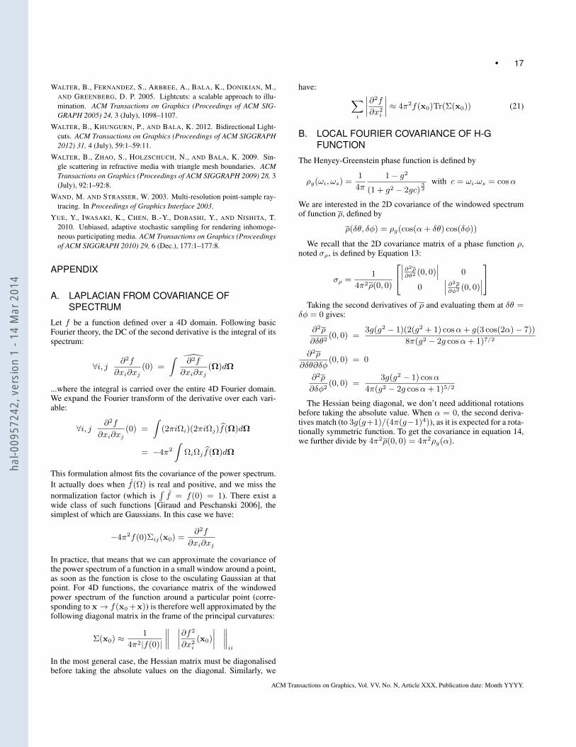
• 17

WALTER, B., FERNANDEZ, S., ARBREE, A., BALA, K., DONIKIAN, M.,AND GREENBERG, D. P. 2005. Lightcuts: a scalable approach to illu-mination. ACM Transactions on Graphics (Proceedings of ACM SIG-GRAPH 2005) 24, 3 (July), 1098–1107.

WALTER, B., KHUNGURN, P., AND BALA, K. 2012. Bidirectional Light-cuts. ACM Transactions on Graphics (Proceedings of ACM SIGGRAPH2012) 31, 4 (July), 59:1–59:11.

WALTER, B., ZHAO, S., HOLZSCHUCH, N., AND BALA, K. 2009. Sin-gle scattering in refractive media with triangle mesh boundaries. ACMTransactions on Graphics (Proceedings of ACM SIGGRAPH 2009) 28, 3(July), 92:1–92:8.

WAND, M. AND STRASSER, W. 2003. Multi-resolution point-sample ray-tracing. In Proceedings of Graphics Interface 2003.

YUE, Y., IWASAKI, K., CHEN, B.-Y., DOBASHI, Y., AND NISHITA, T.2010. Unbiased, adaptive stochastic sampling for rendering inhomoge-neous participating media. ACM Transactions on Graphics (Proceedingsof ACM SIGGRAPH 2010) 29, 6 (Dec.), 177:1–177:8.

APPENDIX

A. LAPLACIAN FROM COVARIANCE OFSPECTRUM

Let f be a function defined over a 4D domain. Following basicFourier theory, the DC of the second derivative is the integral of itsspectrum:

∀i, j ∂2f

∂xi∂xj(0) =

∫∂2f

∂xi∂xj(Ω)dΩ

...where the integral is carried over the entire 4D Fourier domain.We expand the Fourier transform of the derivative over each vari-able:

∀i, j ∂2f

∂xi∂xj(0) =

∫(2πiΩi)(2πiΩj)f(Ω)dΩ

= −4π2

∫ΩiΩj f(Ω)dΩ

This formulation almost fits the covariance of the power spectrum.It actually does when f(Ω) is real and positive, and we miss thenormalization factor (which is

∫f = f(0) = 1). There exist a

wide class of such functions [Giraud and Peschanski 2006], thesimplest of which are Gaussians. In this case we have:

−4π2f(0)Σij(x0) =∂2f

∂xi∂xj

In practice, that means that we can approximate the covariance ofthe power spectrum of a function in a small window around a point,as soon as the function is close to the osculating Gaussian at thatpoint. For 4D functions, the covariance matrix of the windowedpower spectrum of the function around a particular point (corre-sponding to x→ f(x0 +x)) is therefore well approximated by thefollowing diagonal matrix in the frame of the principal curvatures:

Σ(x0) ≈ 1

4π2|f(0)|

∥∥∥∥ ∣∣∣∣∂f2

∂x2i

(x0)

∣∣∣∣ ∥∥∥∥ii

In the most general case, the Hessian matrix must be diagonalisedbefore taking the absolute values on the diagonal. Similarly, we

have: ∑i

∣∣∣∣∂2f

∂x2i

∣∣∣∣ ≈ 4π2f(x0)Tr(Σ(x0)) (21)

B. LOCAL FOURIER COVARIANCE OF H-GFUNCTION

The Henyey-Greenstein phase function is defined by

ρg(ωi, ωs) =1

4π

1− g2

(1 + g2 − 2gc)32

with c = ωi.ωs = cosα

We are interested in the 2D covariance of the windowed spectrumof function ρ, defined by

ρ(δθ, δφ) = ρg(cos(α+ δθ) cos(δφ))

We recall that the 2D covariance matrix of a phase function ρ,noted σρ, is defined by Equation 13:

σρ =1

4π2ρ(0, 0)

∣∣∣ ∂2ρ∂θ2(0, 0)

∣∣∣ 0

0∣∣∣ ∂2ρ∂φ2 (0, 0)

∣∣∣

Taking the second derivatives of ρ and evaluating them at δθ =δφ = 0 gives:

∂2ρ

∂δθ2(0, 0) =

3g(g2 − 1)(2(g2 + 1) cosα+ g(3 cos(2α)− 7))

8π(g2 − 2g cosα+ 1)7/2

∂2ρ

∂δθ∂δφ(0, 0) = 0

∂2ρ

∂δφ2(0, 0) =

3g(g2 − 1) cosα

4π(g2 − 2g cosα+ 1)5/2

The Hessian being diagonal, we don’t need additional rotationsbefore taking the absolute value. When α = 0, the second deriva-tives match (to 3g(g+1)/(4π(g−1)4)), as it is expected for a rota-tionally symmetric function. To get the covariance in equation 14,we further divide by 4π2ρ(0, 0) = 4π2ρg(α).


hal-0

0957

242,

ver

sion

1 -

14 M

ar 2

014

A Local Frequency Analysis of Light Scattering and Absorption

Documents

Transcript of A Local Frequency Analysis of Light Scattering and Absorption