High Frequency Scattering by Convex Polygons Stephen Langdon ...
55
High Frequency Scattering by Convex Polygons Stephen Langdon University of Reading, UK Joint work with: Simon Chandler-Wilde, Steve Arden Funded by: Leverhulme Trust University of Maryland, September 2005 1
-
Upload
khangminh22 -
Category
Documents
-
view
1 -
download
0
Transcript of High Frequency Scattering by Convex Polygons Stephen Langdon ...
High Frequency Scattering by Convex Polygons
Stephen Langdon
University of Reading, UK
Joint work with: Simon Chandler-Wilde, Steve Arden
Funded by: Leverhulme Trust
University of Maryland, September 2005
1
Contents
• The scattering problem
• The Burton & Miller integral equation
• Understanding solution behaviour
• Approximating the solution efficiently
– Galerkin method
– Collocation method
• Numerical Results
2
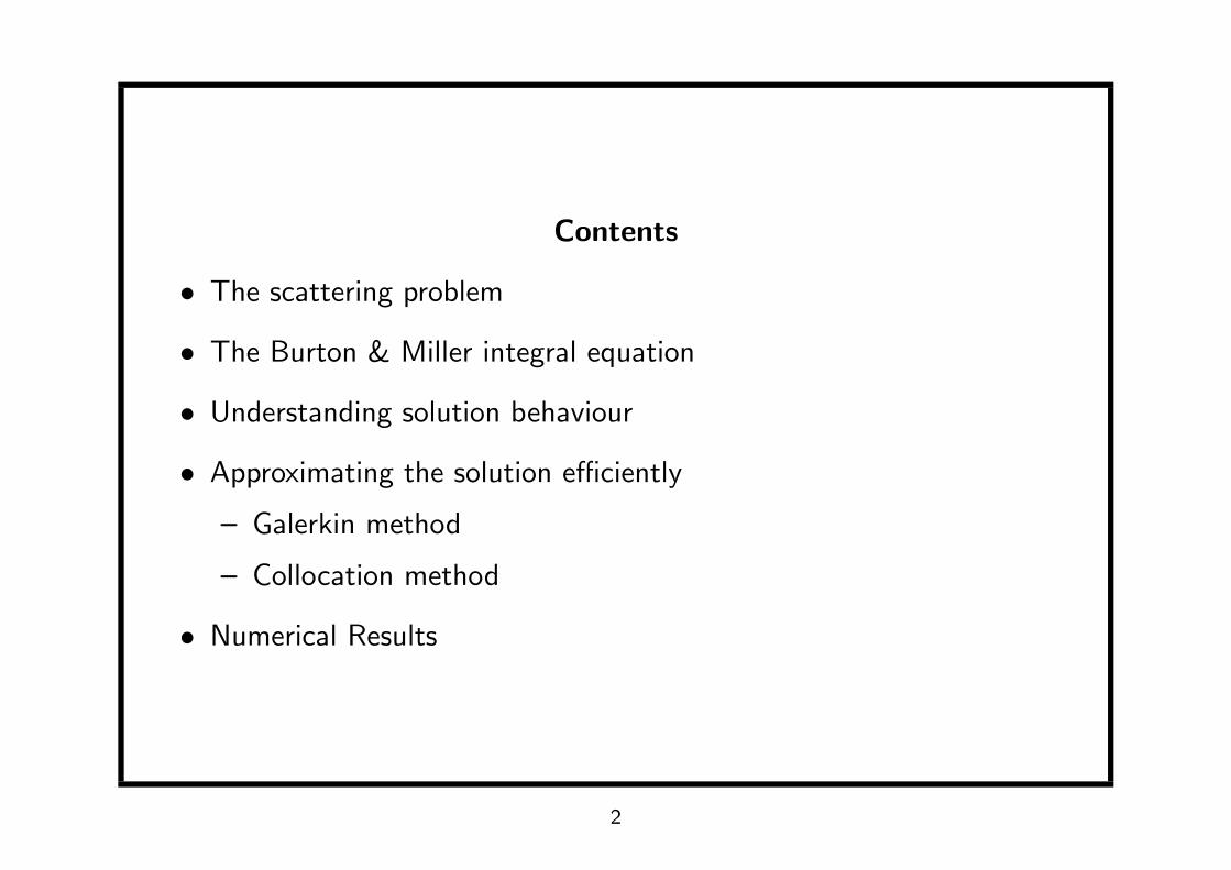
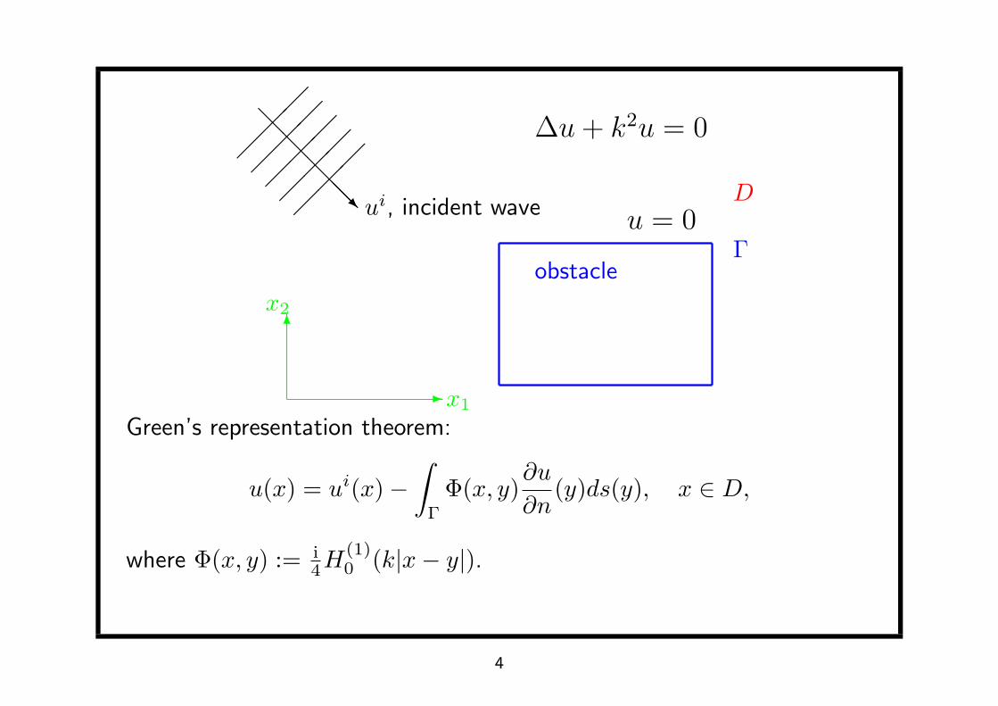
The Scattering Problem
@@
@@@R ui, incident wave
∆u + k2u = 0
u = 0Γ
D
obstacle
-
6
x1
x2
3
@@
@@@R ui, incident wave
∆u + k2u = 0
u = 0Γ
D
obstacle
-
6
x1
x2
Green’s representation theorem:
u(x) = ui(x)−∫
Γ
Φ(x, y)∂u
∂n(y)ds(y), x ∈ D,
where Φ(x, y) := i4H
(1)0 (k|x− y|).
4
@@
@@@R ui, incident wave
∆u + k2u = 0
u = 0Γ
D
obstacle
-
6
x1
x2
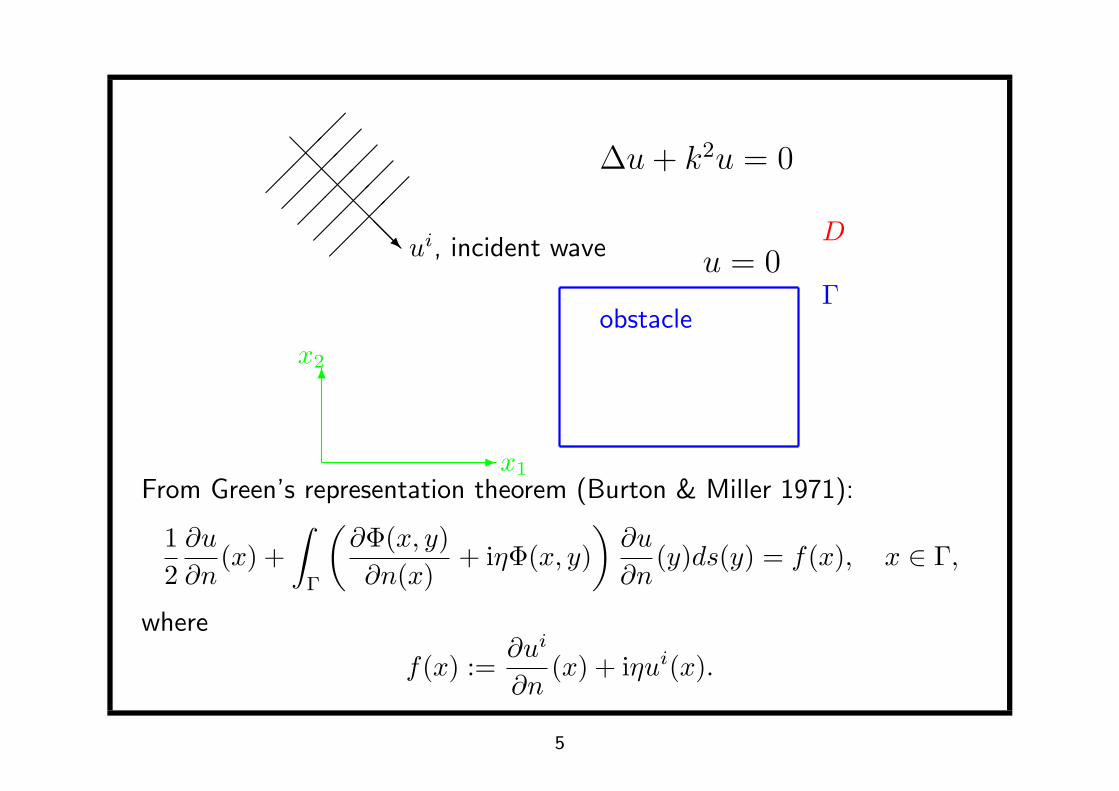
From Green’s representation theorem (Burton & Miller 1971):
12∂u
∂n(x) +
∫Γ
(∂Φ(x, y)∂n(x)
+ iηΦ(x, y))∂u
∂n(y)ds(y) = f(x), x ∈ Γ,
where
f(x) :=∂ui
∂n(x) + iηui(x).
5
@@
@@@R ui, incident wave
∆u + k2u = 0
u = 0Γ
D
2D polygon
-
6
x1
x2
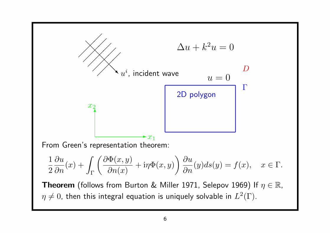
From Green’s representation theorem:
12∂u
∂n(x) +
∫Γ
(∂Φ(x, y)∂n(x)
+ iηΦ(x, y))∂u
∂n(y)ds(y) = f(x), x ∈ Γ.
Theorem (follows from Burton & Miller 1971, Selepov 1969) If η ∈ R,
η 6= 0, then this integral equation is uniquely solvable in L2(Γ).
6
12∂u
∂n(x) +
∫Γ
(∂Φ(x, y)∂n(x)
+ iηΦ(x, y))∂u
∂n(y)ds(y) = f(x), x ∈ Γ.
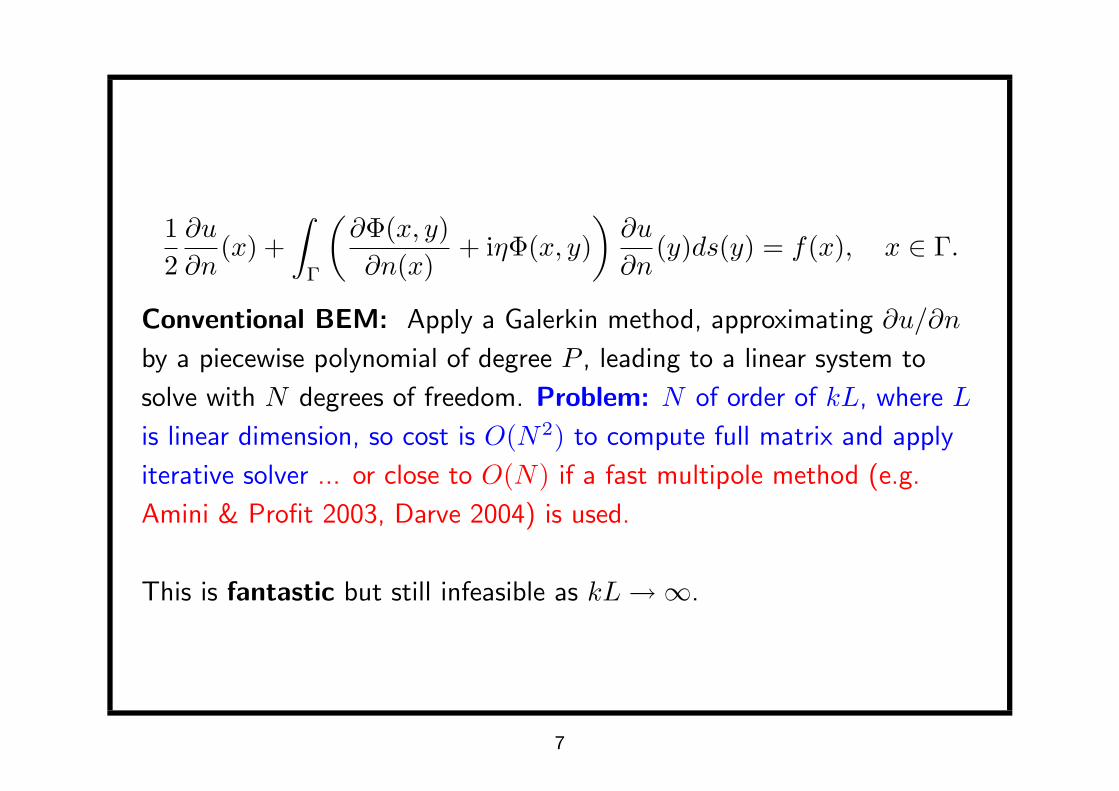
Conventional BEM: Apply a Galerkin method, approximating ∂u/∂n
by a piecewise polynomial of degree P , leading to a linear system to
solve with N degrees of freedom. Problem: N of order of kL, where L
is linear dimension, so cost is O(N2) to compute full matrix and apply
iterative solver ... or close to O(N) if a fast multipole method (e.g.
Amini & Profit 2003, Darve 2004) is used.
This is fantastic but still infeasible as kL→∞.
7
12∂u
∂n(x) +
∫Γ
(∂Φ(x, y)∂n(x)
+ iηΦ(x, y))∂u
∂n(y)ds(y) = f(x), x ∈ Γ.
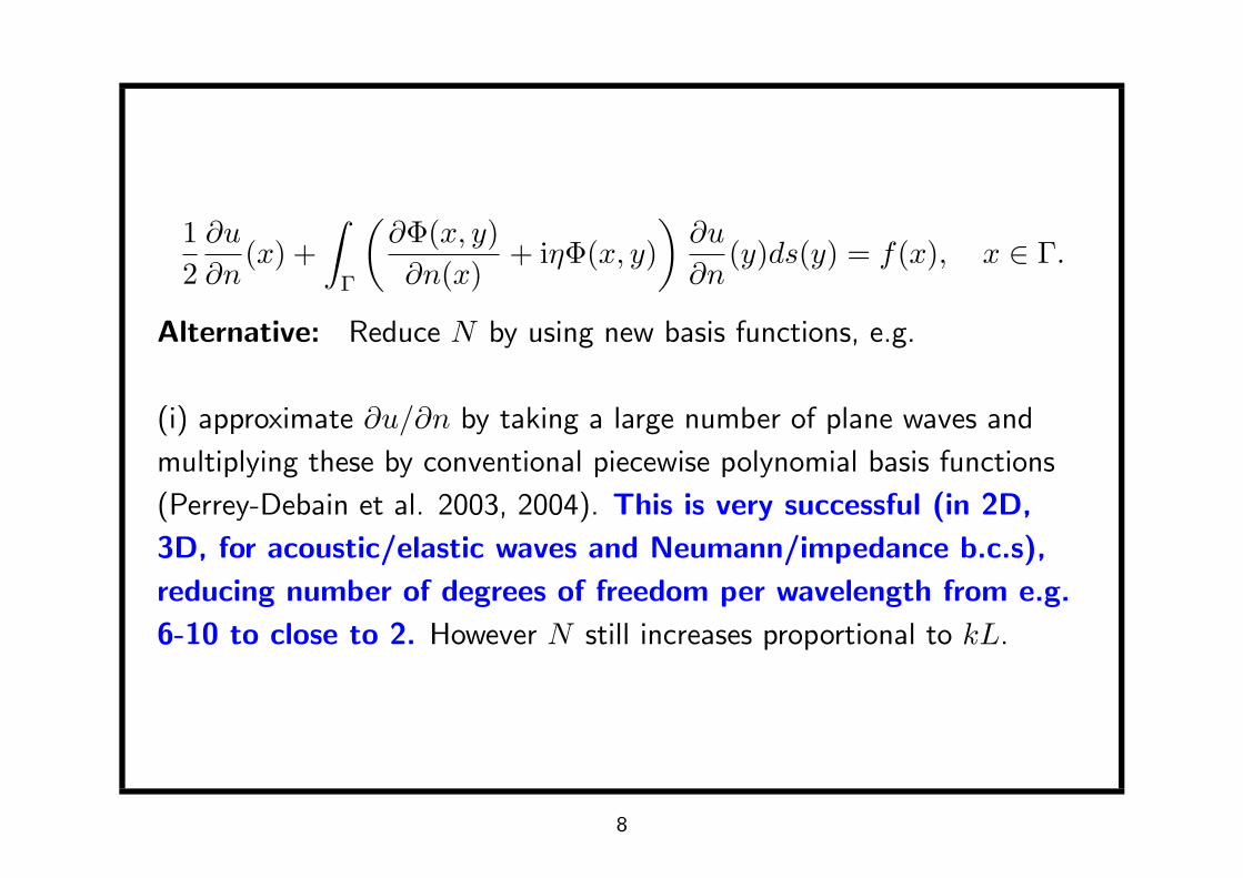
Alternative: Reduce N by using new basis functions, e.g.
(i) approximate ∂u/∂n by taking a large number of plane waves and
multiplying these by conventional piecewise polynomial basis functions
(Perrey-Debain et al. 2003, 2004). This is very successful (in 2D,
3D, for acoustic/elastic waves and Neumann/impedance b.c.s),
reducing number of degrees of freedom per wavelength from e.g.
6-10 to close to 2. However N still increases proportional to kL.
8
12∂u
∂n(x) +
∫Γ
(∂Φ(x, y)∂n(x)
+ iηΦ(x, y))∂u
∂n(y)ds(y) = f(x), x ∈ Γ.
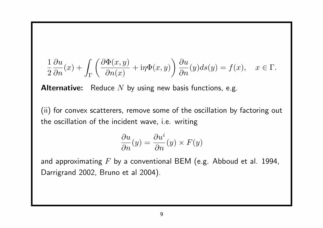
Alternative: Reduce N by using new basis functions, e.g.
(ii) for convex scatterers, remove some of the oscillation by factoring out
the oscillation of the incident wave, i.e. writing
∂u
∂n(y) =
∂ui
∂n(y)× F (y)
and approximating F by a conventional BEM (e.g. Abboud et al. 1994,
Darrigrand 2002, Bruno et al 2004).
9

Alternative: Reduce N by using new basis functions, e.g.
(ii) for convex scatterers, remove some of the oscillation by factoring out
the oscillation of the incident wave, i.e. writing
∂u
∂n(y) =
∂ui
∂n(y)× F (y) (∗)
and approximating F by a conventional BEM.
For smooth obstacles this works well: equation (∗) holds with
F (y) ≈ 2 on the illuminated side (physical optics) and F (y) ≈ 0 in the
shadow zone.
10
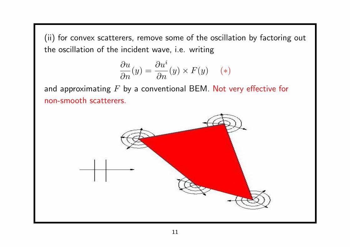
(ii) for convex scatterers, remove some of the oscillation by factoring out
the oscillation of the incident wave, i.e. writing
∂u
∂n(y) =
∂ui
∂n(y)× F (y) (∗)
and approximating F by a conventional BEM. Not very effective for
non-smooth scatterers.
11
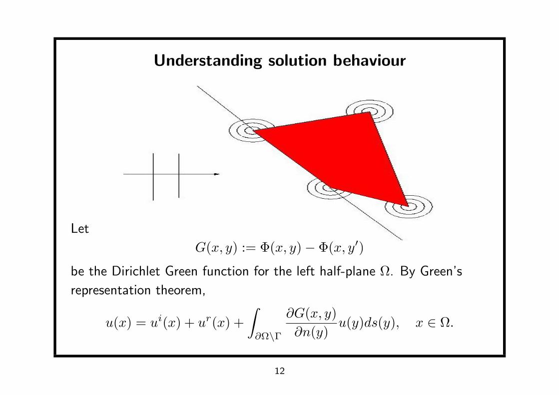
Understanding solution behaviour
Let
G(x, y) := Φ(x, y)− Φ(x, y′)
be the Dirichlet Green function for the left half-plane Ω. By Green’s
representation theorem,
u(x) = ui(x) + ur(x) +∫
∂Ω\Γ
∂G(x, y)∂n(y)
u(y)ds(y), x ∈ Ω.
12
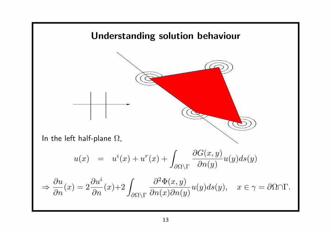
Understanding solution behaviour
In the left half-plane Ω,
u(x) = ui(x) + ur(x) +∫
∂Ω\Γ
∂G(x, y)∂n(y)
u(y)ds(y)
⇒ ∂u
∂n(x) = 2
∂ui
∂n(x)+2
∫∂Ω\Γ
∂2Φ(x, y)∂n(x)∂n(y)
u(y)ds(y), x ∈ γ = ∂Ω∩Γ.
13
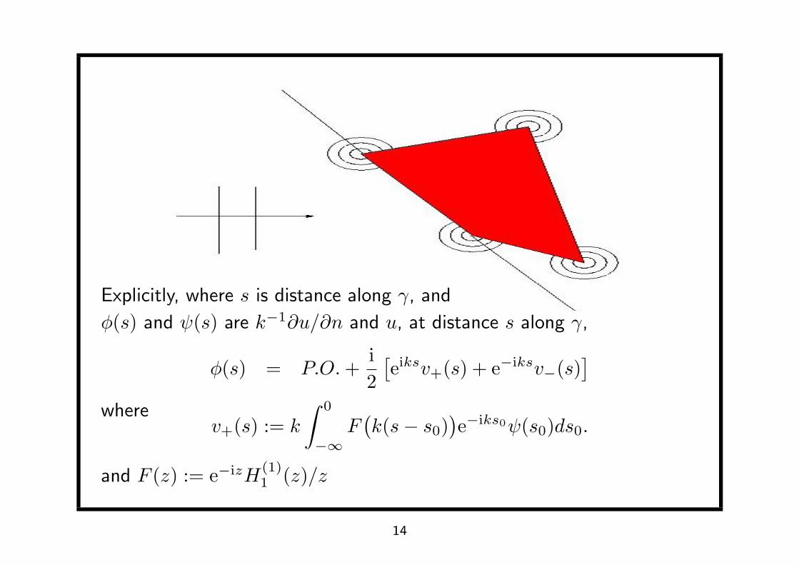
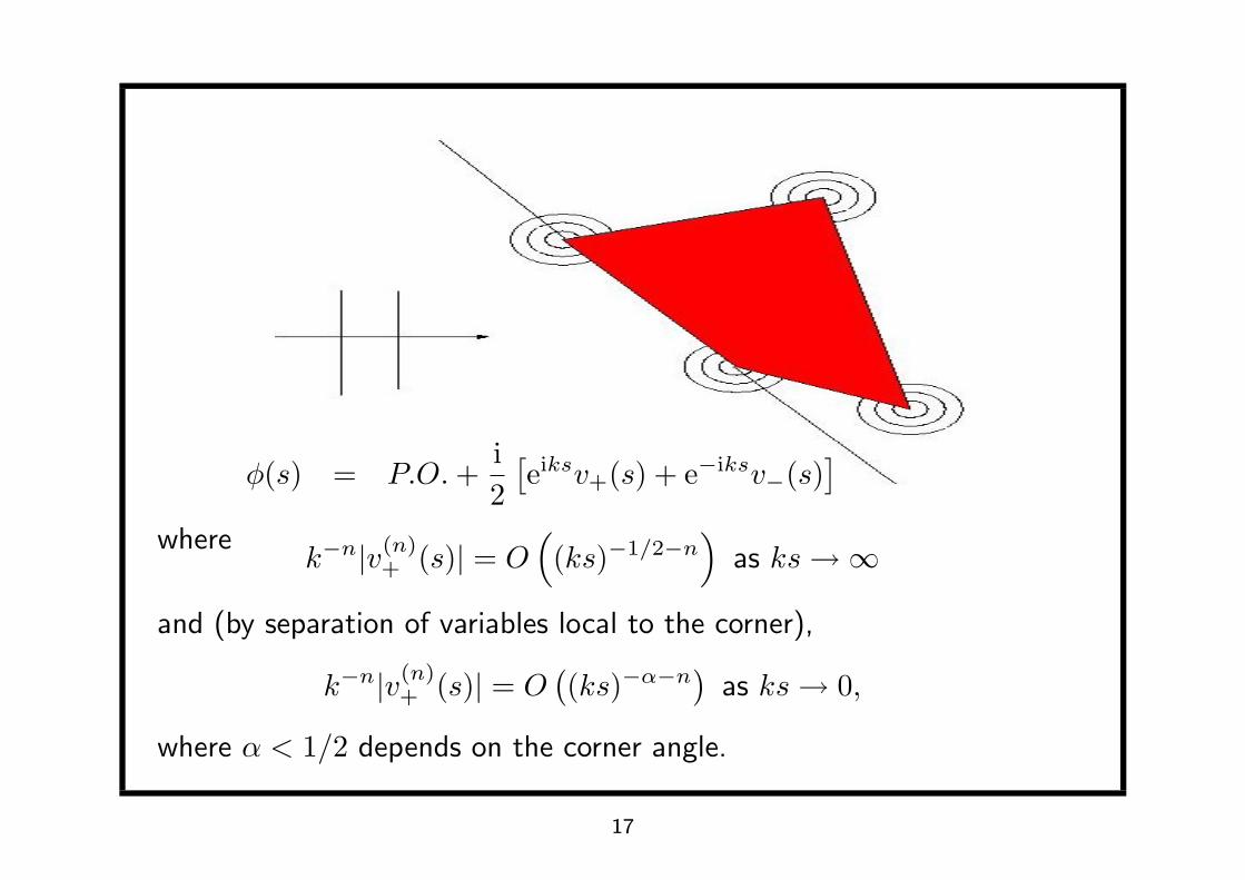
Explicitly, where s is distance along γ, and
φ(s) and ψ(s) are k−1∂u/∂n and u, at distance s along γ,
φ(s) = P.O.+i2
[eiksv+(s) + e−iksv−(s)
]where
v+(s) := k
∫ 0
−∞F
(k(s− s0)
)e−iks0ψ(s0)ds0.
and F (z) := e−izH(1)1 (z)/z
14
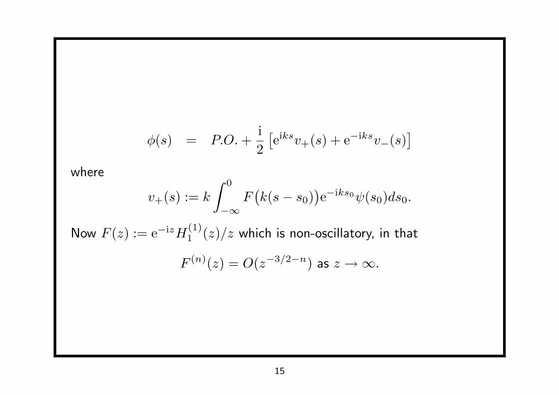
φ(s) = P.O.+i2
[eiksv+(s) + e−iksv−(s)
]where
v+(s) := k
∫ 0
−∞F
(k(s− s0)
)e−iks0ψ(s0)ds0.
Now F (z) := e−izH(1)1 (z)/z which is non-oscillatory, in that
F (n)(z) = O(z−3/2−n) as z →∞.
15
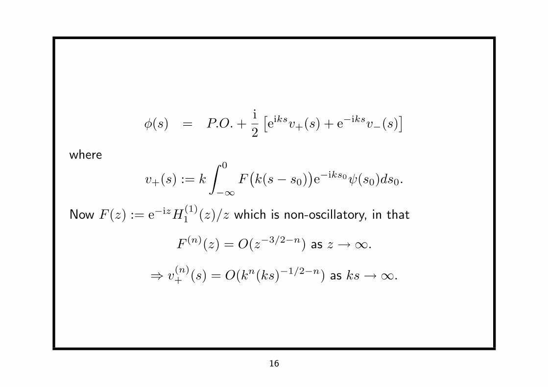
φ(s) = P.O.+i2
[eiksv+(s) + e−iksv−(s)
]where
v+(s) := k
∫ 0
−∞F
(k(s− s0)
)e−iks0ψ(s0)ds0.
Now F (z) := e−izH(1)1 (z)/z which is non-oscillatory, in that
F (n)(z) = O(z−3/2−n) as z →∞.
⇒ v(n)+ (s) = O(kn(ks)−1/2−n) as ks→∞.
16
φ(s) = P.O.+i2
[eiksv+(s) + e−iksv−(s)
]where
k−n|v(n)+ (s)| = O
((ks)−1/2−n
)as ks→∞
and (by separation of variables local to the corner),
k−n|v(n)+ (s)| = O
((ks)−α−n
)as ks→ 0,
where α < 1/2 depends on the corner angle.
17
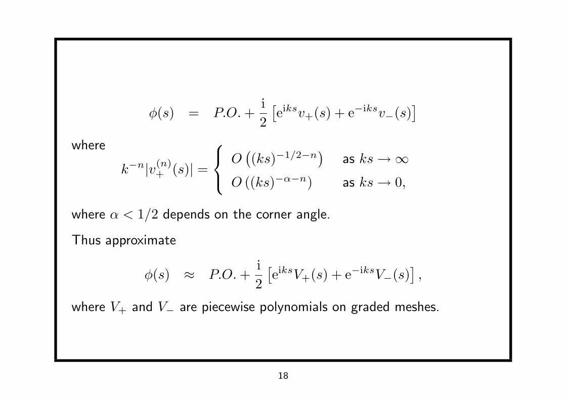
φ(s) = P.O.+i2
[eiksv+(s) + e−iksv−(s)
]where
k−n|v(n)+ (s)| =
O((ks)−1/2−n
)as ks→∞
O ((ks)−α−n) as ks→ 0,
where α < 1/2 depends on the corner angle.
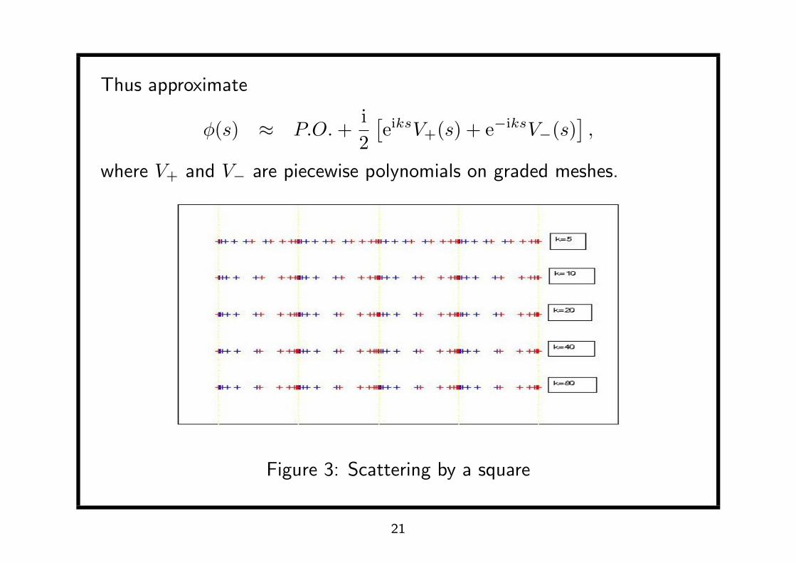
Thus approximate
φ(s) ≈ P.O.+i2
[eiksV+(s) + e−iksV−(s)
],
where V+ and V− are piecewise polynomials on graded meshes.
18
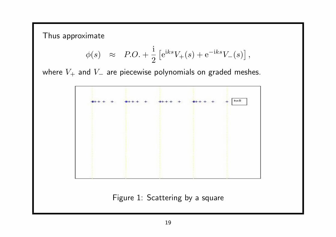
Thus approximate
φ(s) ≈ P.O.+i2
[eiksV+(s) + e−iksV−(s)
],
where V+ and V− are piecewise polynomials on graded meshes.
Figure 1: Scattering by a square
19
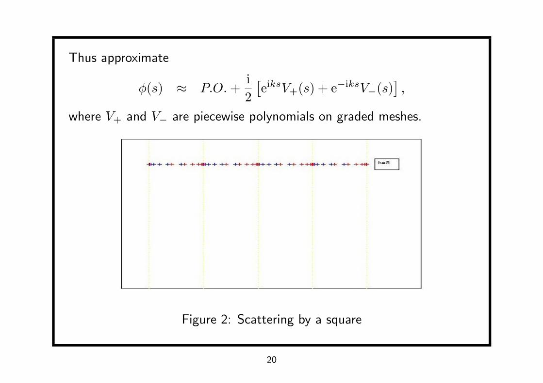
Thus approximate
φ(s) ≈ P.O.+i2
[eiksV+(s) + e−iksV−(s)
],
where V+ and V− are piecewise polynomials on graded meshes.
Figure 2: Scattering by a square
20
Thus approximate
φ(s) ≈ P.O.+i2
[eiksV+(s) + e−iksV−(s)
],
where V+ and V− are piecewise polynomials on graded meshes.
Figure 3: Scattering by a square
21
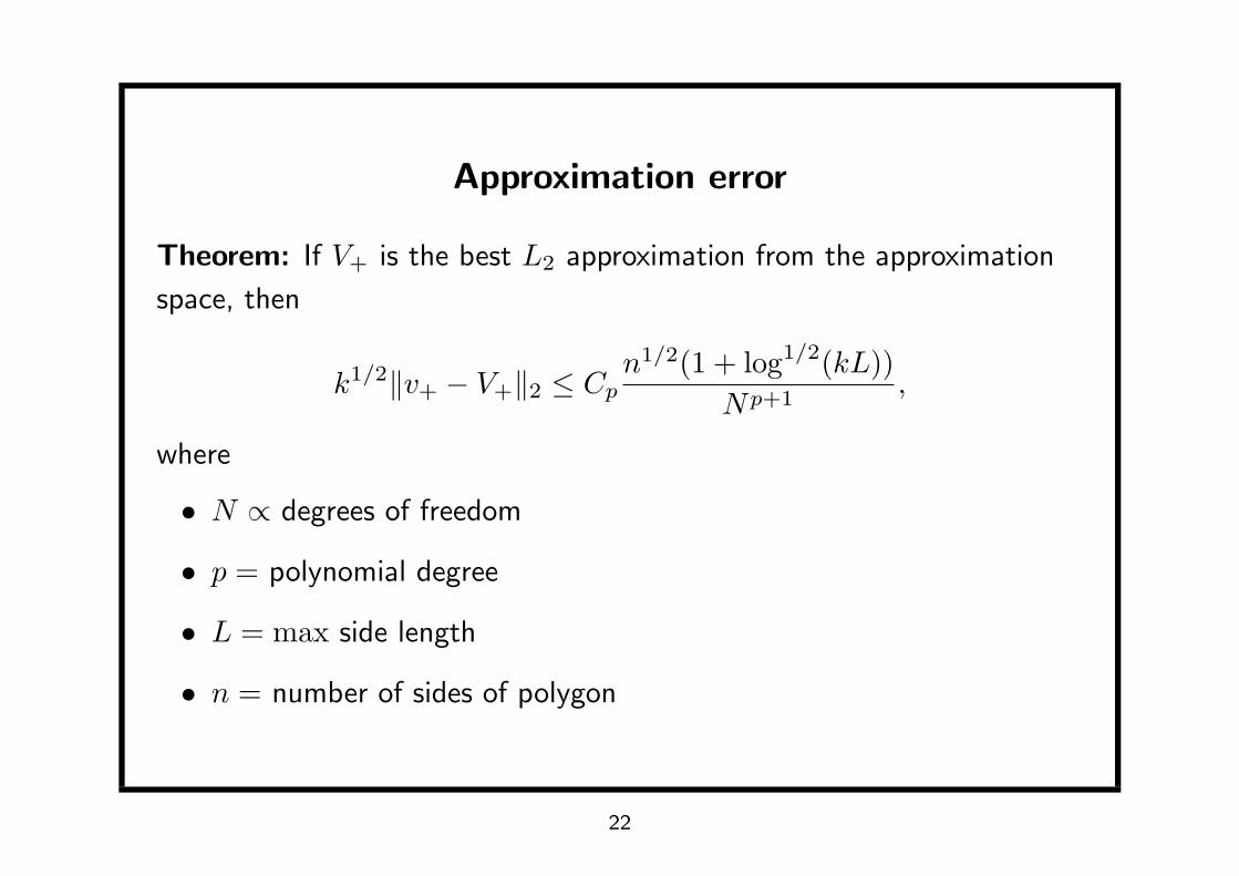
Approximation error
Theorem: If V+ is the best L2 approximation from the approximation
space, then
k1/2‖v+ − V+‖2 ≤ Cpn1/2(1 + log1/2(kL))
Np+1,
where
• N ∝ degrees of freedom
• p = polynomial degree
• L = max side length
• n = number of sides of polygon
22
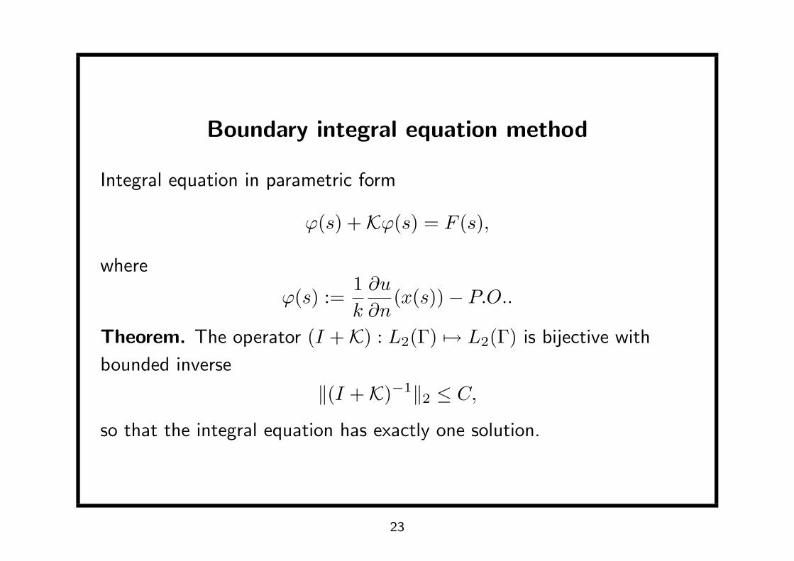
Boundary integral equation method
Integral equation in parametric form
ϕ(s) +Kϕ(s) = F (s),
where
ϕ(s) :=1k
∂u
∂n(x(s))− P.O..
Theorem. The operator (I +K) : L2(Γ) 7→ L2(Γ) is bijective with
bounded inverse
‖(I +K)−1‖2 ≤ C,
so that the integral equation has exactly one solution.
23
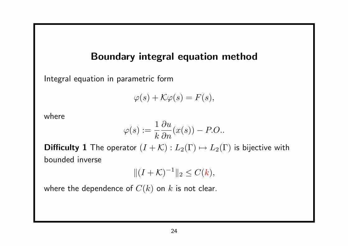
Boundary integral equation method
Integral equation in parametric form
ϕ(s) +Kϕ(s) = F (s),
where
ϕ(s) :=1k
∂u
∂n(x(s))− P.O..
Difficulty 1 The operator (I +K) : L2(Γ) 7→ L2(Γ) is bijective with
bounded inverse
‖(I +K)−1‖2 ≤ C(k),
where the dependence of C(k) on k is not clear.
24
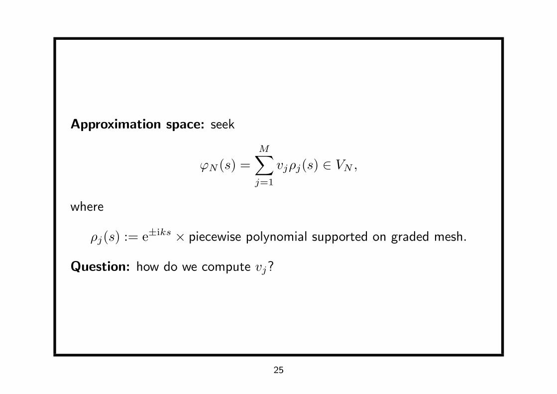
Approximation space: seek
ϕN (s) =M∑
j=1
vjρj(s) ∈ VN ,
where
ρj(s) := e±iks × piecewise polynomial supported on graded mesh.
Question: how do we compute vj?
25
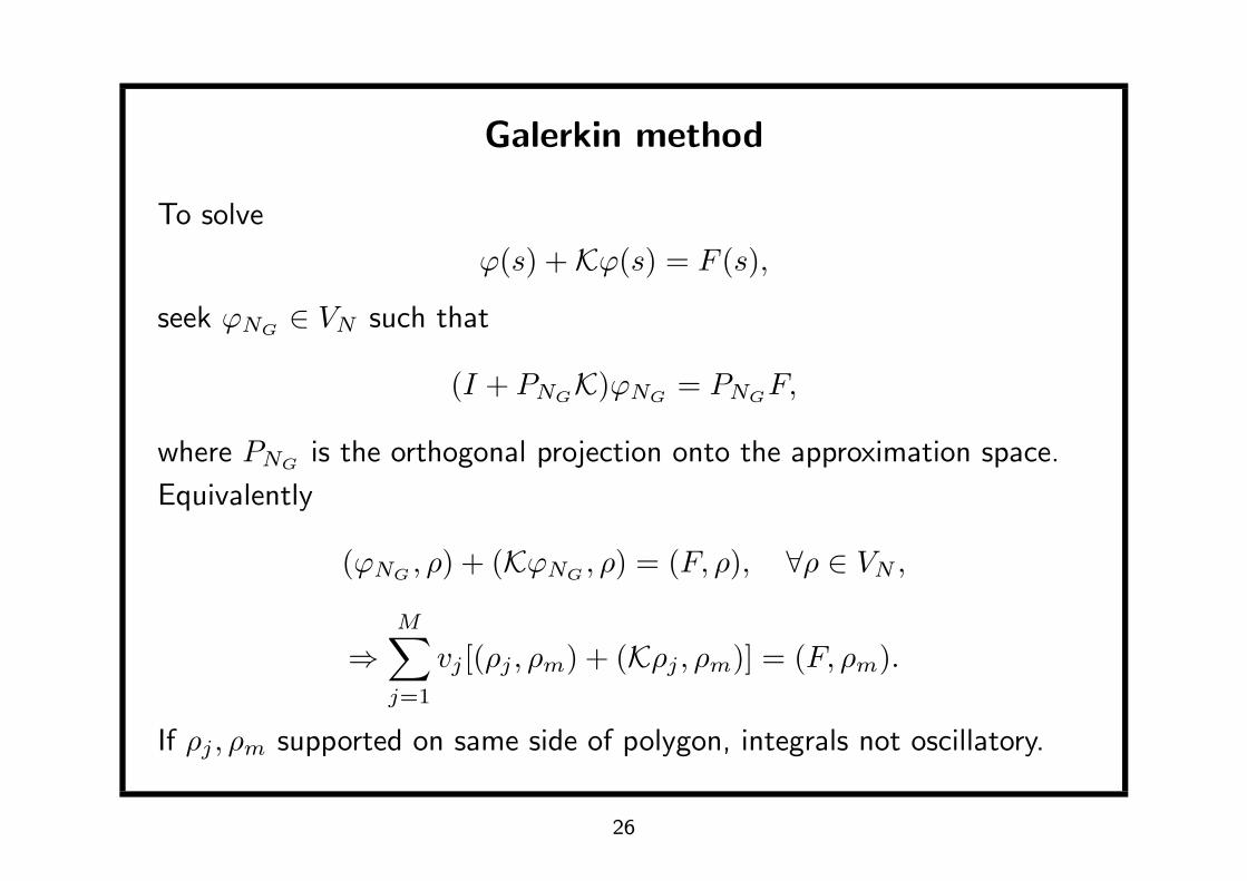
Galerkin method
To solve
ϕ(s) +Kϕ(s) = F (s),
seek ϕNG∈ VN such that
(I + PNGK)ϕNG
= PNGF,
where PNGis the orthogonal projection onto the approximation space.
Equivalently
(ϕNG, ρ) + (KϕNG
, ρ) = (F, ρ), ∀ρ ∈ VN ,
⇒M∑
j=1
vj [(ρj , ρm) + (Kρj , ρm)] = (F, ρm).
If ρj , ρm supported on same side of polygon, integrals not oscillatory.
26
Galerkin method
Theorem. For N ≥ N∗, the operator (I + PNGK) : L2(Γ) 7→ VN is
bijective with bounded inverse
‖(I + PNGK)−1‖2 ≤ Cs.
27
Galerkin method
Difficulty 2. For N ≥ N∗(k), the operator (I + PNGK) : L2(Γ) 7→ VN
is bijective with bounded inverse
‖(I + PNGK)−1‖2 ≤ Cs(k),
where the dependence of N∗(k) and Cs(k) on k is not clear.
28
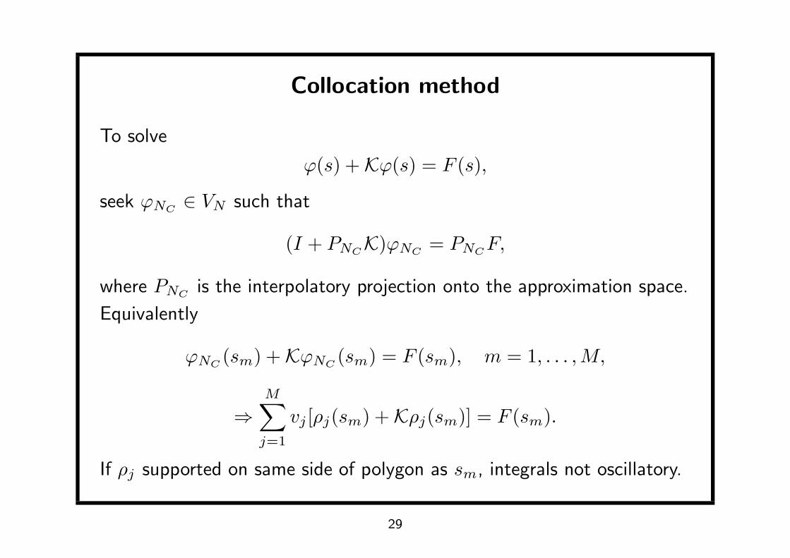
Collocation method
To solve
ϕ(s) +Kϕ(s) = F (s),
seek ϕNC∈ VN such that
(I + PNCK)ϕNC
= PNCF,
where PNCis the interpolatory projection onto the approximation space.
Equivalently
ϕNC(sm) +KϕNC
(sm) = F (sm), m = 1, . . . ,M,
⇒M∑
j=1
vj [ρj(sm) +Kρj(sm)] = F (sm).
If ρj supported on same side of polygon as sm, integrals not oscillatory.
29
Collocation method
We have not shown that (I + PNCK) : L2(Γ) 7→ VN is bijective with
bounded inverse.
30

Galerkin vs. Collocation: error analysis
Theorem There exists a constant Cp > 0, independent of k, such that
for N ≥ N∗
k1/2‖ϕ− ϕNG‖2 ≤ CpCs sup
x∈D|u(x)|n
1/2(1 + log1/2(kL/n))Np+1
,
k1/2|u(x)− uNG(x)| ≤ CpCs sup
x∈D|u(x)|n
1/2(1 + log1/2(kL/n))Np+1
.
• Stability and convergence not proven for collocation scheme.
31
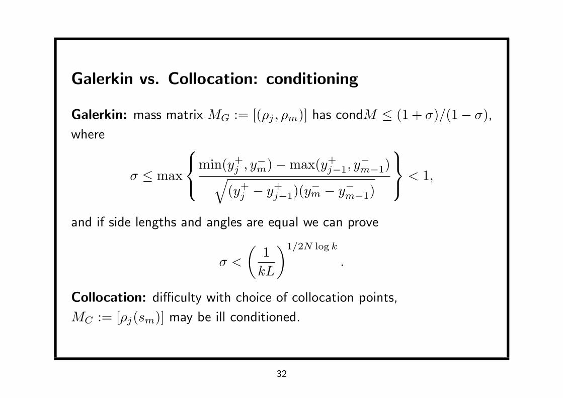
Galerkin vs. Collocation: conditioning
Galerkin: mass matrix MG := [(ρj , ρm)] has condM ≤ (1 + σ)/(1− σ),where
σ ≤ max
min(y+j , y
−m)−max(y+
j−1, y−m−1)√
(y+j − y+
j−1)(y−m − y−m−1)
< 1,
and if side lengths and angles are equal we can prove
σ <
(1kL
)1/2N log k
.
Collocation: difficulty with choice of collocation points,
MC := [ρj(sm)] may be ill conditioned.
32
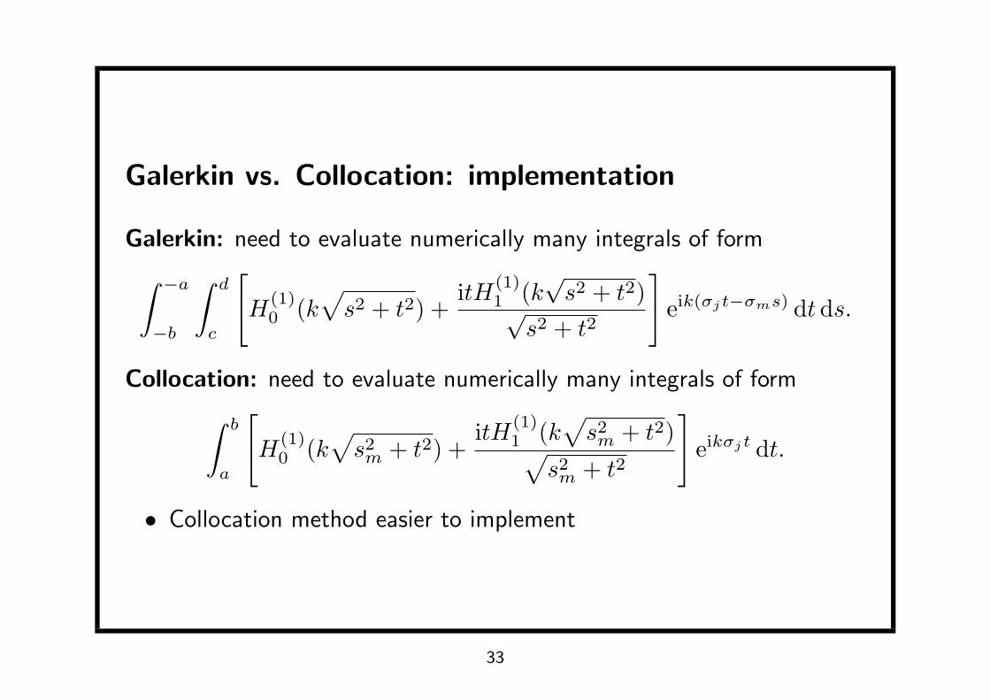
Galerkin vs. Collocation: implementation
Galerkin: need to evaluate numerically many integrals of form∫ −a
−b
∫ d
c
[H
(1)0 (k
√s2 + t2) +
itH(1)1 (k
√s2 + t2)√
s2 + t2
]eik(σjt−σms) dtds.
Collocation: need to evaluate numerically many integrals of form∫ b
a
[H
(1)0 (k
√s2m + t2) +
itH(1)1 (k
√s2m + t2)√
s2m + t2
]eikσjt dt.
• Collocation method easier to implement
33
Numerical results
scattering by a square, k = 5
scattering by a square, k = 10
34
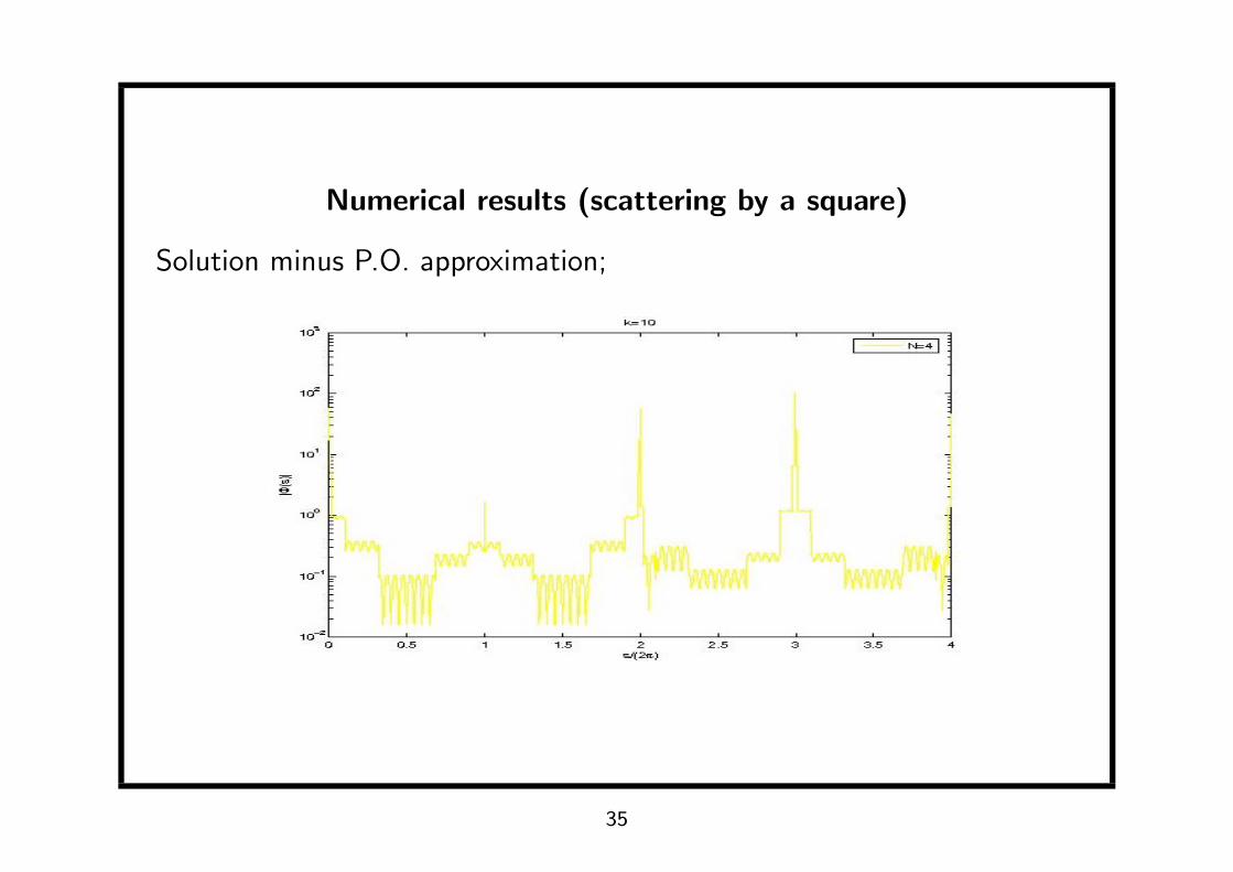
Numerical results (scattering by a square)
Solution minus P.O. approximation;
35
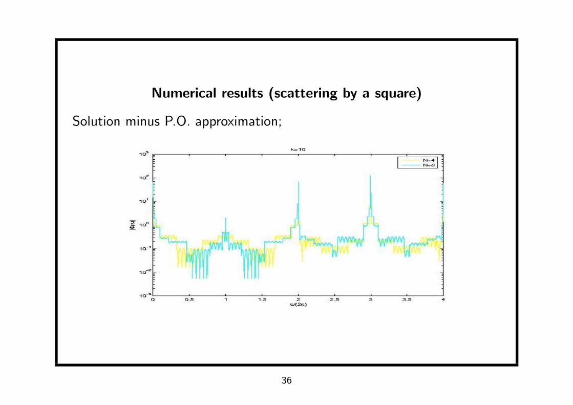
Numerical results (scattering by a square)
Solution minus P.O. approximation;
36
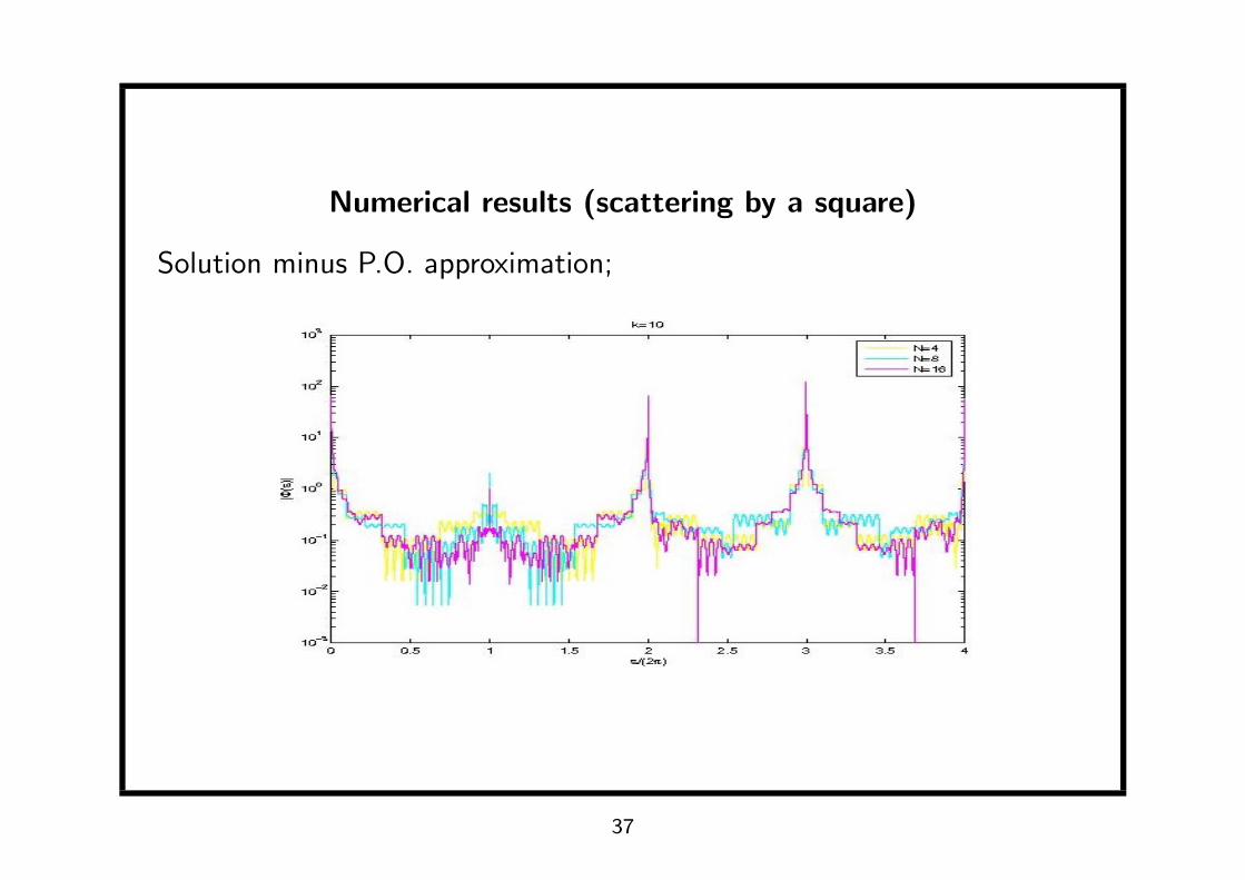
Numerical results (scattering by a square)
Solution minus P.O. approximation;
37
Numerical results (scattering by a square)
Solution minus P.O. approximation;
38
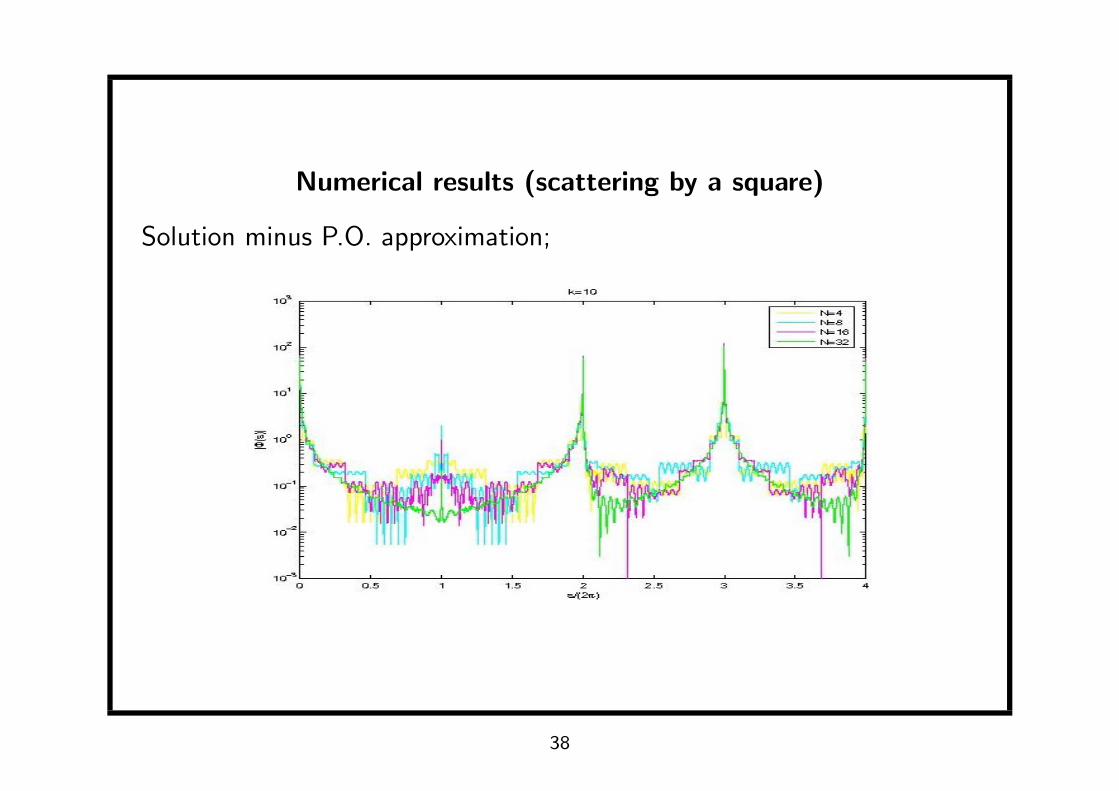
Numerical results (scattering by a square)
Solution minus P.O. approximation;
39
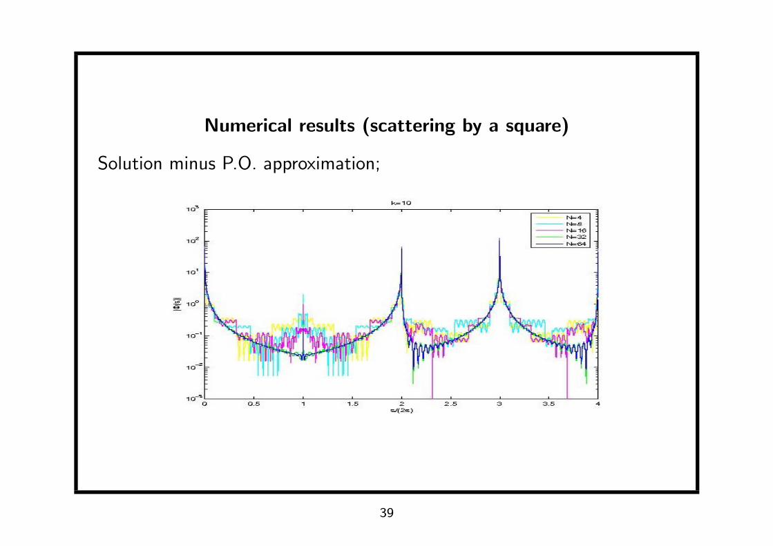
Numerical results (scattering by a square)
Solution minus P.O. approximation;
40
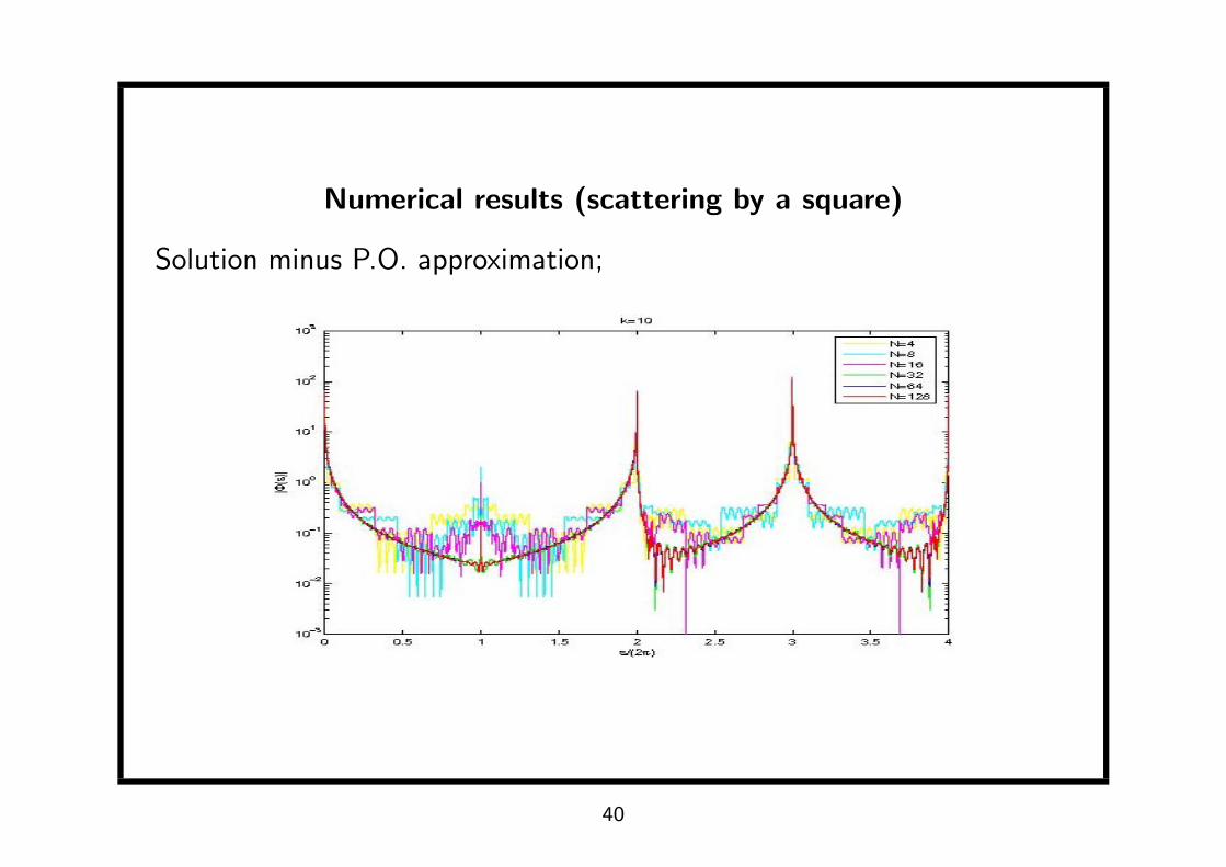
Numerical results (scattering by a square)
Solution minus P.O. approximation;
41
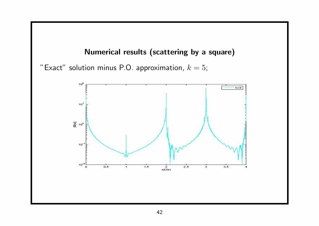
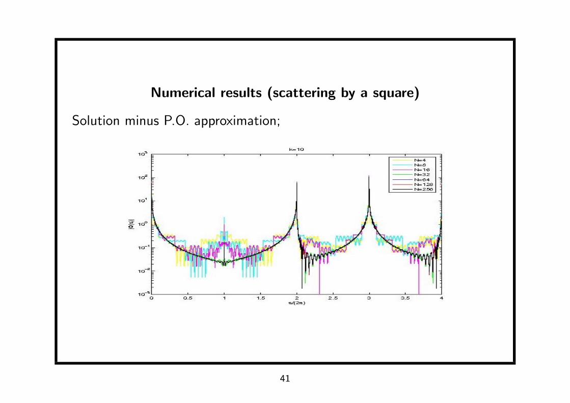
Numerical results (scattering by a square)
”Exact” solution minus P.O. approximation, k = 5;
42
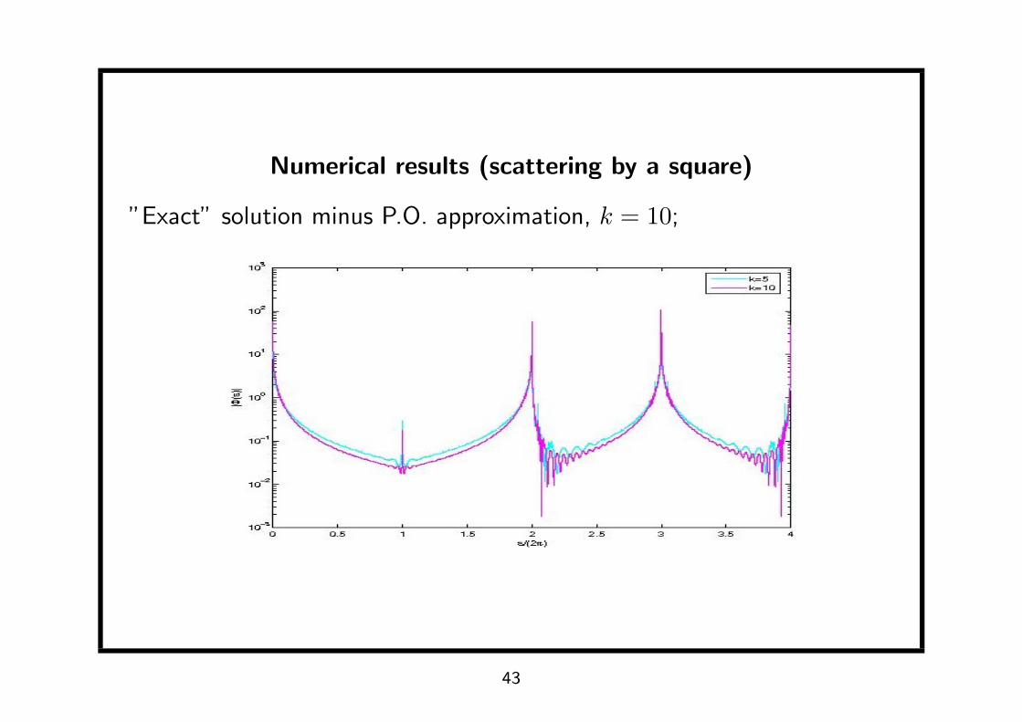
Numerical results (scattering by a square)
”Exact” solution minus P.O. approximation, k = 10;
43

Numerical results (scattering by a square)
”Exact” solution minus P.O. approximation, k = 20;
44
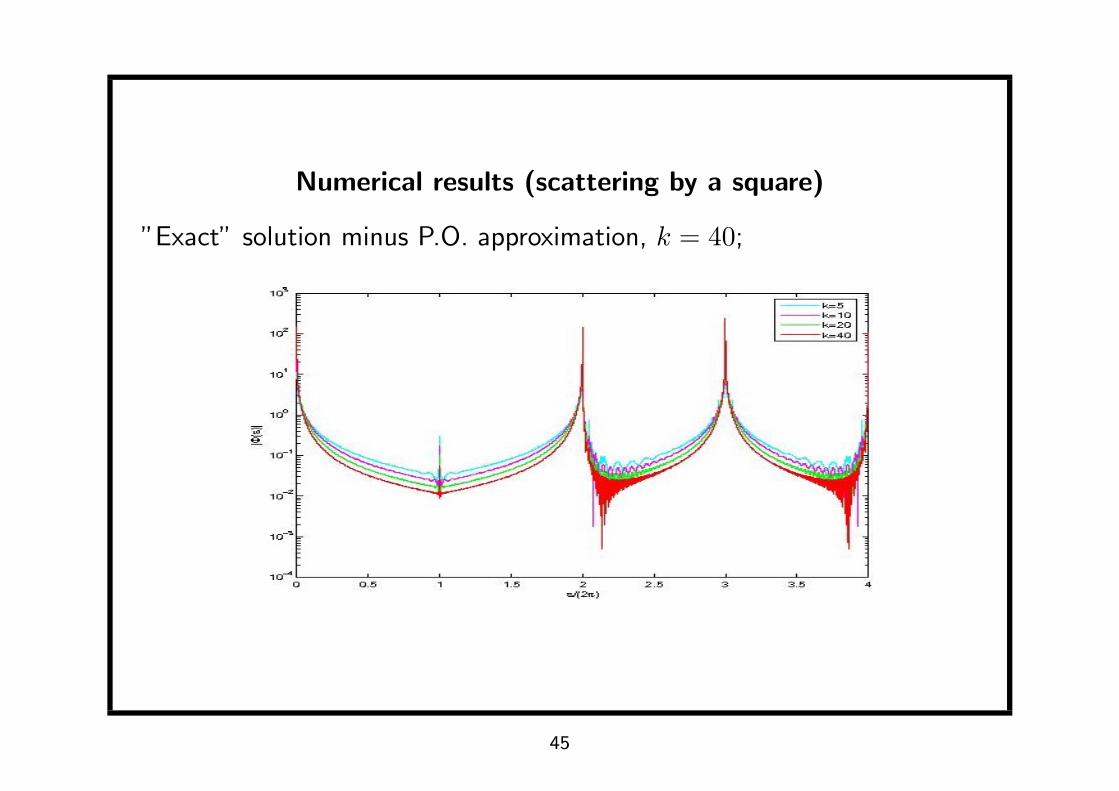
Numerical results (scattering by a square)
”Exact” solution minus P.O. approximation, k = 40;
45

Table 1: Relative errors, k = 10
k N dof‖ϕ−ϕNG
‖2‖ϕ‖2
‖ϕ−ϕNC‖2
‖ϕ‖2
10 2 24 1.1691×10+0 7.5453×10⁻¹
4 48 4.3784×10⁻¹ 4.7335×10⁻¹
8 96 2.2320×10⁻¹ 2.6980×10⁻¹
16 192 1.2106×10⁻¹ 1.2670×10⁻¹
32 376 1.1633×10⁻¹ 6.8440×10⁻²
64 752 2.8702×10⁻² 3.3034×10⁻²
46

Table 2: Relative errors, k = 160
k N dof‖ϕ−ϕNG
‖2‖ϕ‖2
‖ϕ−ϕNC‖2
‖ϕ‖2
160 2 32 7.2765×10⁻¹ 6.8901×10⁻¹
4 56 4.2628×10⁻¹ 4.4455×10⁻¹
8 112 4.9060×10⁻¹ 4.6445×10⁻¹
16 224 1.2847×10⁻¹ 2.3456×10⁻¹
32 456 8.4578×10⁻² 9.3327×10⁻²
64 904 3.4570×10⁻² 4.8153×10⁻²
47
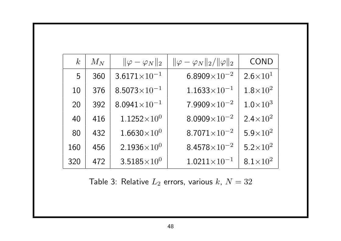
k MN ‖ϕ− ϕN‖2 ‖ϕ− ϕN‖2/‖ϕ‖2 COND
5 360 3.6171×10⁻¹ 6.8909×10⁻² 2.6×101
10 376 8.5073×10⁻¹ 1.1633×10⁻¹ 1.8×10²
20 392 8.0941×10⁻¹ 7.9909×10⁻² 1.0×10³
40 416 1.1252×100 8.0909×10⁻² 2.4×10²
80 432 1.6630×100 8.7071×10⁻² 5.9×10²
160 456 2.1936×100 8.4578×10⁻² 5.2×10²
320 472 3.5185×100 1.0211×10⁻¹ 8.1×10²
Table 3: Relative L2 errors, various k, N = 32
48
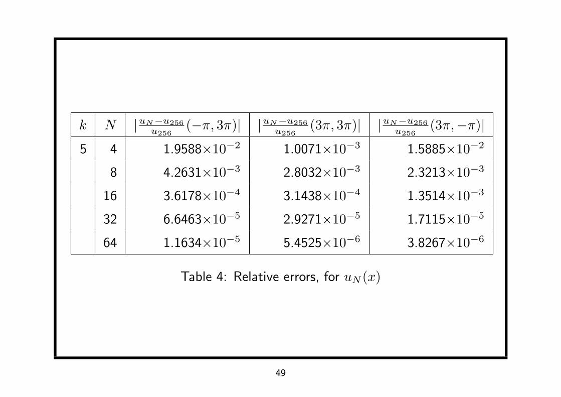
k N |uN−u256u256
(−π, 3π)| |uN−u256u256
(3π, 3π)| |uN−u256u256
(3π,−π)|
5 4 1.9588×10⁻² 1.0071×10⁻³ 1.5885×10⁻²
8 4.2631×10⁻³ 2.8032×10⁻³ 2.3213×10⁻³
16 3.6178×10⁻⁴ 3.1438×10⁻⁴ 1.3514×10⁻³
32 6.6463×10⁻⁵ 2.9271×10⁻⁵ 1.7115×10⁻⁵
64 1.1634×10⁻⁵ 5.4525×10⁻⁶ 3.8267×10⁻⁶
Table 4: Relative errors, for uN (x)
49
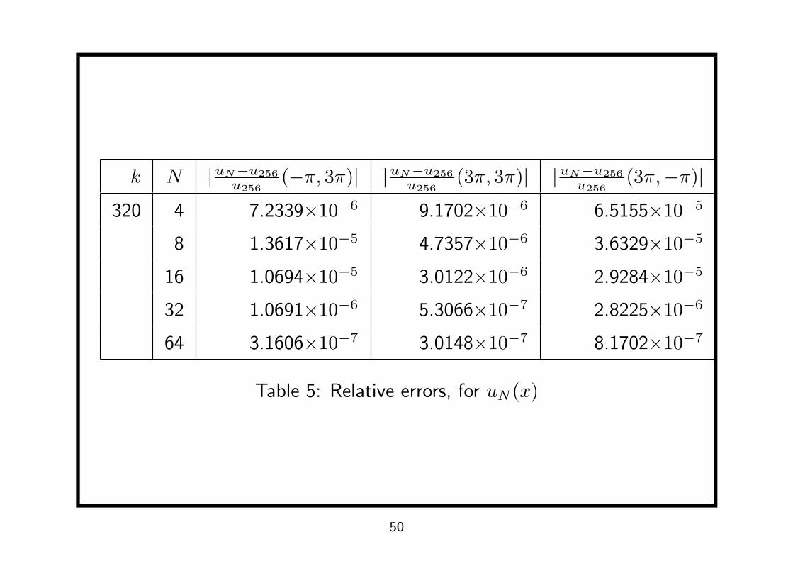
k N |uN−u256u256
(−π, 3π)| |uN−u256u256
(3π, 3π)| |uN−u256u256
(3π,−π)|
320 4 7.2339×10⁻⁶ 9.1702×10⁻⁶ 6.5155×10⁻⁵
8 1.3617×10⁻⁵ 4.7357×10⁻⁶ 3.6329×10⁻⁵
16 1.0694×10⁻⁵ 3.0122×10⁻⁶ 2.9284×10⁻⁵
32 1.0691×10⁻⁶ 5.3066×10⁻⁷ 2.8225×10⁻⁶
64 3.1606×10⁻⁷ 3.0148×10⁻⁷ 8.1702×10⁻⁷
Table 5: Relative errors, for uN (x)
50

What we actually are computing . . .
The difference between the exact solution and a leading order
approximation;
Figure 4: square, k = 5
51
What we actually are computing . . .
The difference between the exact solution and a leading order
approximation;
Figure 5: square, k = 10
52

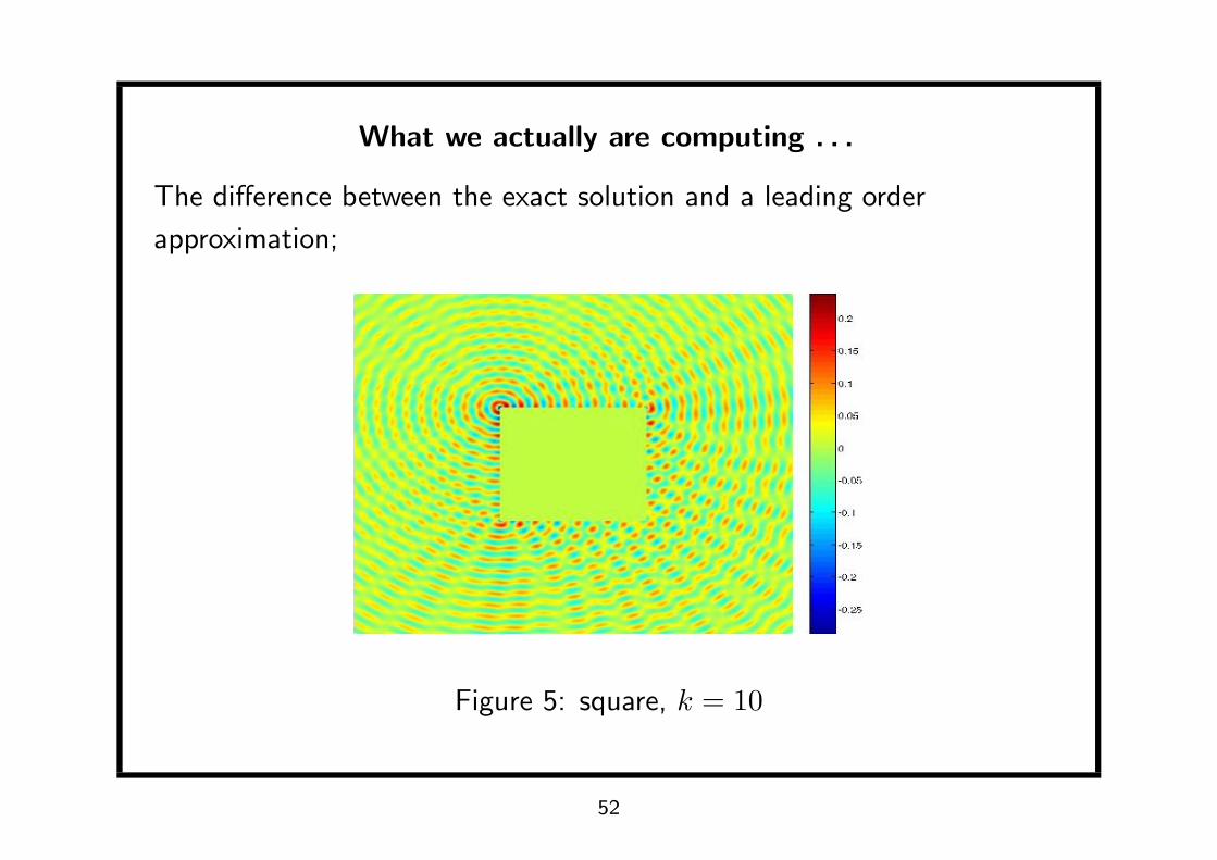
What we actually are computing . . .
The difference between the exact solution and a leading order
approximation;
Figure 6: square, k = 20
53
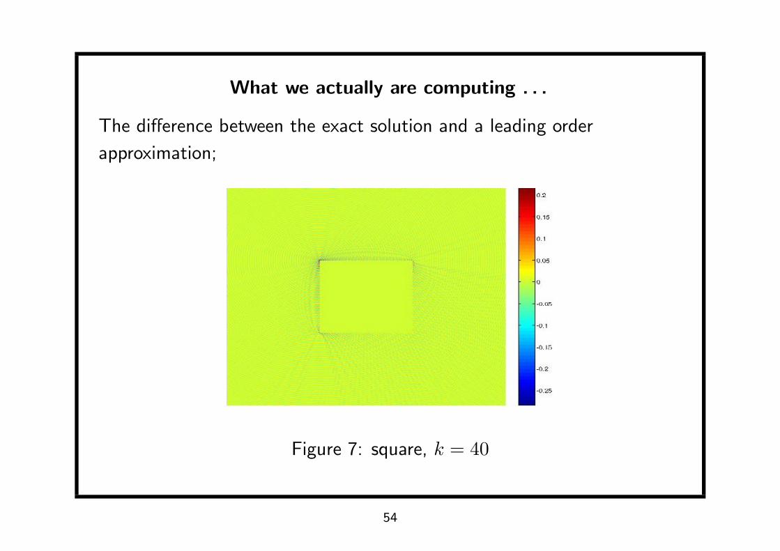
What we actually are computing . . .
The difference between the exact solution and a leading order
approximation;
Figure 7: square, k = 40
54
Summary and Conclusions
• Using Green’s representation theorem in a half-plane we can
understand behaviour of the field on the boundary and its
derivatives for scattering by a convex polygon (extends to convex
polyhedron in 3D)
• For a convex polygon, design of an optimal graded mesh for
piecewise polynomial approximation is then straightforward
• The number of degrees of freedom need only grow logarithmically
with the wavenumber to maintain a fixed accuracy
• Ongoing considerations
– Galerkin vs. Collocation - stability and convergence analysis
– Better schemes for evaluating oscillatory integrals
– hp ideas
55


![MATH-G Exam [E-24EKGT] Polygons and Circles Packet](https://static.fdokumen.com/doc/165x107/63156d0415106505030ba4e9/math-g-exam-e-24ekgt-polygons-and-circles-packet.jpg)