arX

iv:1

107.

2422

v1 [

cs.D

S] 1

2 Ju

l 201

1

A Linear Time Algorithm for Seeds Computation

(Full Version)

Tomasz Kociumaka∗ Marcin Kubica∗ Jakub Radoszewski∗

Wojciech Rytter ∗† Tomasz Walen∗

Abstract

Periodicity in words is one of the most fundamental areas of text algorithms and combi-natorics. Two classical and natural variations of periodicity are seeds and covers (also calledquasiperiods). Linear-time algorithms are known for finding all the covers of a word, howeverin case of seeds, for the past 15 years only an O(n logn) time algorithm was known (Iliopoulos,Moore and Park, 1996). Finding an o(n log n) time algorithm for the all-seeds problem was men-tioned as one of the most important open problems related to repetitions in words in a surveyby Smyth (2000). We show a linear-time algorithm computing all the seeds of a word, in par-ticular, the shortest seed. Our approach is based on the use of a version of LZ-factorization andnon-trivial combinatorial relations between the LZ-factorization and seeds. It is used here forthe first time in context of seeds. It saves the work done for factors processed earlier, similarlyas in Crochemore’s square-free testing.

Keywords: seed in a word, Lempel-Ziv factorization, suffix tree

∗Dept. of Mathematics, Computer Science and Mechanics, University of Warsaw, Warsaw, Poland,

[kociumaka,kubica,jrad,rytter,walen]@mimuw.edu.pl†Dept. of Math. and Informatics, Copernicus University, Torun, Poland

1

1 Introduction

The notion of periodicity in words is widely used in many fields, such as combinatorics on words,pattern matching, data compression, automata theory formal language theory, molecular biologyetc. (see [26]). The concept of quasiperiodicity is a generalization of the notion of periodicity,and was defined by Apostolico & Ehrenfeucht in [1]. A quasiperiodic word is entirely covered byoccurrences of another (shorter) word, called the quasiperiod or the cover. The occurrences ofthe quasiperiod may overlap, while in a periodic repetition the occurrences of the period do notoverlap. Hence, quasiperiodicity enables detecting repetitive structure of words when it cannot befound using the classical characterizations of periods. An extension of the notion of a cover is thenotion of a seed — a cover which is not necessarily aligned with the ends of the word being covered,but is allowed to overflow on either side. Seeds were first introduced and studied by Iliopoulos,Moore and Park [20].

Covers and seeds have potential applications in DNA sequence analysis, namely in the search forregularities and common features in DNA sequences. The importance of the notions of quasiperiod-icity follows also from their relation to text compression. Due to natural applications in molecularbiology (a hybridization approach to analysis of a DNA sequence), both covers and seeds have alsobeen extended in the sense that a set of factors are considered instead of a single word [22]. Thisway the notions of k-covers [8, 19], λ-covers [17] and λ-seeds [16] were introduced. In applicationssuch as molecular biology and computer-assisted music analysis, finding exact repetitions is not al-ways sufficient, the same problem holds for quasiperiodic repetitions. This lead to the introductionof the notions of approximate covers [29] and approximate seeds [6].

1.1 Previous results

Iliopoulos, Moore and Park [20] gave an O(n log n) time algorithm computing all the seeds of agiven word w ∈ Σn. For the next 15 years, no o(n log n) time algorithm was known for this problem.Computing all the seeds of a word in linear time was also set as an open problem in the survey [30].A parallel algorithm computing all the seeds in O(log n) time and O(n1+ǫ) space using n processorsin the CRCW PRAM model was given by Berkman et al. [3]. An alternative sequential O(n log n)algorithm for computing the shortest seed was recently given by Christou et al. [7].

In contrast, a linear time algorithm finding the shortest cover of a word was given by Apostolicoet al. [2] and later on improved into an on-line algorithm by Breslauer [4]. A linear time algorithmcomputing all the covers of a word was proposed by Moore & Smyth [28]. Afterwards an on-linealgorithm for the all-covers problem was given by Li & Smyth [25].

Another line of research is finding maximal quasiperiodic subwords of a word. This notionresembles the maximal repetitions (runs) in a word [23], which is another widely studied notionof combinatorics on words. O(n log n) time algorithms for reporting all maximal quasiperiodicsubwords of a word of length n have been proposed by Brodal & Pedersen [5] and Iliopoulos &Mouchard [21], these results improved upon the initial O(n log2 n) time algorithm by Apostolico &Ehrenfeucht [1].

1.2 Our results

We present a linear time algorithm computing a linear representation of all the seeds of a word. Ouralgorithm runs in linear time due to combinatorics on words: the connections between seeds andfactorizations stated in the following Reduction-Property Lemma and Work-Skipping Lemma; andalgorithmics: linear time implementation of merging smaller results into larger, due to efficient

2

Figure 1: The word abaa is the shortest seed of the word aaabaabaabaaabaaba.

processing of subtrees of a suffix tree (the function ExtractSubtrees), and efficient computation oflong candidates for seeds (the function ComputeInRange).

An important tool used in the paper is the f -factorization which is a variant of the Lempel-Zivfactorization [31]. It plays an important role in optimization of text algorithms (see [9, 24, 27]).Intuitively, we can save some work, reusing the results computed for the previous occurrences offactors. We also apply this technique here. The f -factorization can be computed in linear time[11, 13], using so called Longest Previous non-overlapping Factor (LPnF ) table.

Another important text processing tool is the suffix tree [10, 12]. The suffix tree of a word is acompact TRIE of all the suffixes of the word. The suffix tree can be constructed in O(n) time foran integer alphabet Σ (directly [14] or from the suffix array [10, 12]).

In the algorithm we assume that the alphabet Σ consists of integers, and its size is polynomialin n. Hence, the letters of w can be sorted in linear time.

1.3 Preliminaries

We consider words over Σ, u ∈ Σ∗; the positions in u are numbered from 1 to |u|. By Σn we denotethe set of words of length n. For u = u1u2 . . . un, let us denote by u[i . . j] a factor of u equal toui . . . uj.

We say that a word v is a cover of w (covers w) if every letter of w is within some occurrenceof v as a subword of w. A word v is a seed of w if it is a subword of w and w is a subword of someword u covered by v, see Fig. 1. The following lemma provides a useful property of covers whichwe will use also for seeds.

Lemma 1. If v is a cover of w then there exists a sequence of at most⌊

2 |w||v|

⌋

occurrences of v

which completely covers w.

Proof. The proof goes by induction over |w|. If |w| ≤ 2 |v| then the conclusion holds, since v isboth a prefix and a suffix of w. Otherwise, let i be the starting position of the last occurrence of vin w such that i ≤ |v|. Now let j be the first position of the next occurrence of v in w. Note thatboth positions i, j exist and that j > |v|.

The word v is a cover of w[j . . |w|]. By the inductive hypothesis, w[j . . |w|] can be covered by at

most⌊

2(|w|−j+1)|v|

⌋

=⌊

2 |w||v|

⌋

− 2 occurrences of v. Hence, w can be covered by all these occurrences

together with those starting at 1 and at i. This concludes the inductive proof.

2 The tools: factorizations and staircases

From now on, let us fix a word w ∈ Σn. The intervals [i . . j] = i, i + 1, . . . , j will be denoted bysmall Greek letters. Assume all intervals considered satisfy 1 ≤ i ≤ j ≤ n. We denote by |γ| thelength of the interval γ.

By a factorization of a word w we mean a sequence F = (f1, f2, . . . , fK) of factors of w suchthat w = f1f2 . . . fK and for each i = 1, 2, . . . ,K, fi is a subword of f1 . . . fi−1 or a single letter.Denote |F | = K. A factorization of w is called an f -factorization [10] if F has the minimal numberof factors among all the factorizations of w. An f -factorization is constructed in a greedy way, as

3

follows. Let 1 ≤ i ≤ K and j = |f1f2 . . . fi−1| + 1. If w[j] occurs in f1f2 . . . fi−1, then fi is thelongest prefix of w[j . . |w|] that is a subword of w[1 . . j − 1]. Otherwise fi = w[j].

There is a useful relation between covers and f -factorization, which then extends for seeds (seethe Quasiseeds-Factors Lemma in the next section). For a factorization F and interval λ, denoteby Fλ the set of factors of F which start and end within λ.

Lemma 2. Let F be an f -factorization of w and v be a cover of w. Then for λ = [|v| + 1 . . |w|]we have:

|Fλ| ≤⌊

2 |w||v|

⌋

.

Proof. We assume that |w| > |v|, otherwise the conclusion is trivial. By Lemma 1, the word w canbe completely covered with some occurrences of v at the positions i1, i2, . . . , ip, 1 = i1 < i2 < . . . <

ip, where p ≤⌊

2 |w||v|

⌋

. Additionally define ip+1 = |w|+ 1. Then there exists a factorization F ′ of w

such that:F ′λ = w[|v| + 1 . . i3 − 1] ∪ w[ij . . ij+1 − 1] : j = 3, 4, . . . , p.

This set forms a factorization of w[|v| + 1 . . |w|] and consists of p − 1 elements. This concludesthat for any f -factorization of w the set Fλ consists of at most p− 1 elements, since otherwise wecould substitute all the elements from this set by F ′

λ, shorten the rightmost element of F \ Fλ tothe position |v| and thus transform F into a factorization of w with a smaller number of factors,which is not possible.

Another useful concept is that of a staircase of intervals. An interval staircase covering w is asequence of intervals of length 3m with overlaps of size 2m, starting at the beginning of w; possiblythe last interval is shorter. More formally, an m-staircase covering w for a given 1 ≤ m ≤ n, is aset of intervals covering w, defined as follows:

S =

[k ·m+ 1 . . (k + 3) ·m− 1] ∩ [1 . . n], for k = 0, 1, . . . ,max(

0,⌈ n

m

⌉

− 3)

\ ∅.

A first informal description of the algorithm: The main algorithm finding the seedsworks recursively. The computation for the whole word w is reduced to the computation for severalsubwords of w. One could try to use the subwords corresponding to an interval staircase S, howeverthis would not bring any gain in the time complexity, since the total length of the intervals fromS could be about 3n. Instead, in the algorithm a reduced staircase K is used for determining therecursive calls (the definition of this notion follows). By the following Reduction-Property Lemma,for a smart choice of the parameter m the total length of the intervals in K is less than 1

2n, whichis very important in the analysis of the time complexity of the whole algorithm.

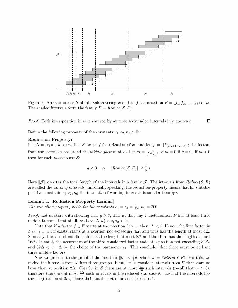
Let F = (f1, f2, . . . , fK) be an f -factorization of w. If S is an m-staircase covering w, let Kbe the family of those intervals λ = [i . . j] ∈ S, that w[i . . j +m] (an extended interval) does notlie within a single factor of F , that is w[i . . j + m] overlaps more than one factor of F . Then wesay that K is obtained by a reduction of S with regard to the f -factorization F and denote this byK = Reduce(S, F ).

There is a simple and useful relation between this reduction and the number of factors in agiven factorization.

Lemma 3. [Staircase-Factors Lemma]Assume we have an m-staircase S covering w and any factorization F of w. Then

|Reduce(S, F )| ≤ 4 (|F | − 1).

4

w :

S :

f1 f2 f3 f4 f5 f6 f7 f8

Figure 2: An m-staircase S of intervals covering w and an f -factorization F = (f1, f2, . . . , f8) of w.The shaded intervals form the family K = Reduce(S, F ).

Proof. Each inter-position in w is covered by at most 4 extended intervals in a staircase.

Define the following property of the constants c1, c2, n0 > 0:

Reduction-Property:Let ∆ = ⌊c1n⌋, n > n0. Let F be an f -factorization of w, and let g = |F[2∆+1..n−∆]|; the factors

from the latter set are called the middle factors of F . Let m =⌊

c2ng

⌋

, or m = 0 if g = 0. If m > 0

then for each m-staircase S:

g ≥ 3 ∧ ‖Reduce(S, F )‖ <1

2n.

Here ‖J ‖ denotes the total length of the intervals in a family J . The intervals from Reduce(S, F )are called the working intervals. Informally speaking, the reduction-property means that for suitablepositive constants c1, c2, n0 the total size of working intervals is smaller than 1

2n.

Lemma 4. [Reduction-Property Lemma]The reduction-property holds for the constants c1 = c2 =

150 , n0 = 200.

Proof. Let us start with showing that g ≥ 3, that is, that any f -factorization F has at least threemiddle factors. First of all, we have ∆(n) > c1n0 > 0.

Note that if a factor f ∈ F starts at the position i in w, then |f | < i. Hence, the first factor inF[2∆+1..n−∆], if exists, starts at a position not exceeding 4∆, and thus has the length at most 4∆.Similarly, the second middle factor has the length at most 8∆ and the third has the length at most16∆. In total, the occurrence of the third considered factor ends at a position not exceeding 32∆,and 32∆ < n −∆ by the choice of the parameter c1. This concludes that there must be at leastthree middle factors.

Now we proceed to the proof of the fact that ‖K‖ < 12n, where K = Reduce(S, F ). For this, we

divide the intervals from K into three groups. First, let us consider intervals from K that start nolater than at position 2∆. Clearly, in S there are at most 2∆

msuch intervals (recall that m > 0),

therefore there are at most 2∆m

such intervals in the reduced staircase K. Each of the intervals hasthe length at most 3m, hence their total length does not exceed 6∆.

5

Figure 3: A word w of length n with a f -factorization F = (f1, f2, . . . , f12). Here the middle factorsof F are: f7, f8, f9, f10, so g = 4. The segments above illustrate the family K = Reduce(S, F ). Bythe Reduction-Property Lemma, if these segments are short enough and ∆ is small enough, thenthe total length of these intervals, ‖K‖, does not exceed 1

2n.

Now consider the intervals from K which end at some position ≥ n−∆+1. Each of the intervalsstarts at the position not smaller than:

n−∆+ 1− 3m+ 1 ≥ n−∆(n) + 2− 3∆g

≥ n− 2∆ + 2.

In the second inequality we used the fact that g ≥ 3. Hence, all the considered intervals from Kare subintervals of an interval of length 2∆. Exactly in the same way as in the previous case weobtain that their total length does not exceed 6∆.

Finally, we consider the intervals from K which are subintervals of an interval

α = [2∆ + 1 . . n−∆] .

Let S ′ be the set of intervals obtained from S by extending each interval by m positions to theright. Let fi, fi+1, . . . , fj be all the factors of F with a non-empty intersection with the interval α.Note that j + 1− i ≤ g + 2. Then, due to the Staircase-Factors Lemma, we have:

|λ ∈ K : λ ⊆ α| = |Reduce(S, (fi, . . . , fj))| ≤ 4(g + 1).

The total length of such intervals does not exceed:

4 · (g + 1) · 3m ≤ gm(

12 + 1g

)

< 13 · c2n.

Here, again, we used the fact that g ≥ 3.In conclusion, we have:

‖K‖ < 2 · 6 · c1n+ 13 · c2n < 12n.

From now on we fix the values of the constants c1, c2, n0 as in Lemma 4.

3 Quasiseeds

Assume v is a subword of w. If w can be decomposed into w = xyz, where |x|, |z| < |v| and v is acover of y, then we say that v is a quasiseed of w. On the other hand, if w can be decomposed intow = xyz, so that |x|, |z| < |v| and v is a seed of w1vw3, then v is a border seed of w. We have thefollowing simple observation.

Observation 1. Let v be a subword of w. The word v is a seed of w if and only if v is a quasiseedof w and v is a border seed of w.

6

A quasiseed is a weaker and computationally easier version of the seed, the main part of thealgorithm computes representations of all the quasiseeds. Then from this information the seeds canbe computed in linear time, applying the border seed condition, by already known methods [7, 20].We describe this step in Subsection 3.2.

As a corollary of Lemma 2, we obtain a similar fact for quasiseeds (hence, also for seeds).

Lemma 5. [Quasiseeds-Factors Lemma]Let F be an f -factorization of w and v be a quasiseed of w. Then for α = [2 |v|+ 1 . . |w| − |v|] wehave:

|Fα| ≤⌊

2 |w||v|

⌋

.

A direct consequence of this lemma is one of key facts used to save the work of the algorithm.Due to this fact we can skip a large part of computations.

Lemma 6. [Work-Skipping Lemma]Let c1, c2, n0 be as in Lemma 4. Let g be the number of middle factors in an f -factorization F ofthe word w, w ∈ Σn for n > n0. Then there is no quasiseed v of w such that

2n

g< |v| ≤ c1n. (1)

Proof. Assume to the contrary that there exists a quasiseed v which satisfies the conditions (1). Bythe Quasiseeds-Factors Lemma we obtain that |Fα| · |v| ≤ 2 |w| where α = [2 |v|+1 . . |w|−|v|]. Dueto the condition |v| ≤ c1n = ∆, we have |Fα| ≥ |F[2∆+1..n−∆]| = g. We conclude that g · |v| ≤ 2 |w|,which contradicts the first inequality from (1).

3.1 Quasigaps

The suffix tree of the word w, denoted as T , is a compact TRIE of all suffixes of the word w#,for # /∈ Σ being a special end-marker. Recall that a suffix tree can be constructed in O(n) time[10, 12, 14]. For simplicity, we identify the nodes of T (both explicit and implicit) with the subwordof w which they represent. Leaves of T correspond to suffixes of w; the leaf corresponding tow[i . . n] is annotated with i.

Let us introduce an equivalence relation on subwords of w. We say that two words are equivalentif the sets of start positions of their occurrences as subwords of w are equal. Note that this relationis very closely bonded with the suffix tree. Namely, each equivalence class corresponds to the set ofimplicit nodes lying on the same edge together with the explicit deeper end of that edge. Quasiseedsbelonging to the same equivalence class turn out to have a regular structure. To describe it, let usintroduce the notion of quasigap, a key one for our algorithm.

Definition 1. Let v be a subword of w. If v is a quasiseed of w, then by quasigap(v) we denote thelength of the shortest quasiseed of w equivalent to v. Otherwise we define quasigap(v) as ∞.

The following observation provides a characterization of all quasiseeds of a given word using onlythe quasigaps of explicit nodes in the suffix tree T .

Observation 2. All quasiseeds in a given equivalence class are exactly the prefixes of the longestword v in this class (corresponding to an explicit node in the suffix tree) of length at least quasigap(v).

Proof. Let u and u′ be equivalent to v and such that |u| < |u′|. It suffices to show that if u is aquasiseed, then so is u′. Indeed, since the sets of occurrences of both words are equal, this is a clearconsequence of the definition of a quasiseed.

7

Example 1. Consider the words w = aaaaaabaaabaaabaaaa, v = aaabaaa. The equivalence classof v is E = aaabaaa, aaabaa, aaaba, aaab. In E quasiseeds are aaabaaa, aaabaa, aaaba. Amongthese quasiseeds only v is a border seed of w, hence a seed of w (in this case the only one). Allquasiseeds in E are the prefixes of v of length at least 5, hence quasigap(v) = 5.

3.2 From quasigaps to seeds

In this section we show how to reduce finding all seeds of w.to computing quasigaps. For this, dueto Observation 1, we need to identify all border seeds among quasiseeds of w. By Observation 2,the set of quasiseeds consists of a family of ranges v[1 . . k] : quasigap(v) ≤ k ≤ |v| on an edge(u, v) of T . We call such a range a candidate set.

The approach presented in [20] (section “Finding hard seeds”) can now be used. This algorithmtakes as its input all candidate sets of w and of wR, where wR is the reversed w. It returns allthe seeds of w represented as ranges on the edges of suffix trees of both w and wR. Alternatively,one can exploit an algorithm presented in [7], which, given a family of candidate sets of w, finds ashortest border seed of w belonging to this family, hence a shortest seed.

Both solutions run in linear time. Therefore, we have reduced the problem of finding seeds tocomputing quasigaps of explicit nodes in T . Hence, as soon as we show that this can be done inO(n) time (Theorem 2), we obtain the main result of the paper.

Theorem 1. An O(n)-size representation of all the seeds of w can be found in O(n) time. Inparticular, a shortest seed can be computed within the same time complexity.

4 Generalization to arbitrary intervals

The algorithm computing quasigaps (which are a representation of quasiseeds) has a recursivestructure. Unfortunately, the relation between quasiseeds in subwords of w and quasiseeds of entirew is quite subtle and we have to deal with technical representations of quasiseeds on the suffix tree.Even worse, the suffix trees of subwords of w are not exactly subtrees of the suffix tree of w. Dueto these issues, our algorithm operates on subintervals of [1 . . n] rather than subwords of w.

For an interval γ = [i . . j], we can introduce the notions of an f -factorization, an intervalstaircase covering γ and a reduced staircase in a natural way exactly as the corresponding notionsfor the subword w[i . . j].

4.1 Induced suffix trees

Let us define an induced suffix tree T (γ) for γ = [i . . j]. It is obtained from T as follows. First,leaves labelled with numbers from γ and all their ancestors are selected, and all other nodes areremoved. Then, the resulting tree is compacted, that is, all non-branching nodes become implicit.Still, the nodes (implicit and explicit) of such a tree can be identified with subwords of w. Ofcourse, T (γ) is not a suffix tree of w[i . . j].

By Nodes(T (γ)) we denote the set of explicit nodes of T (γ). Let v be a (possibly implicit) nodeof T (γ). By parent (v, γ) we denote the closest explicit ancestor of v. We assume that the rootthe only node that is an ancestor of itself. Additionally, for an implicit node v of T (γ), we definedesc(v, γ) as the closest explicit descendant of v. If v is explicit we assume desc(v, γ) = v.

8

4.2 Quasigaps in an arbitrary interval

Here we extend the notion of quasigaps to a given interval γ. We provide definitions which aretechnically more complicated, however computationally more useful.

Before that we need to develop some notation. Let v be an arbitrary subword of w, or equiva-lently a node of T . By Occ(v, γ) we denote the set of those starting positions of occurrences of vthat lie in the interval γ. Note that the set Occ(v, γ) represents the set of all leaves of T (γ) in thesubtree rooted at v. Let first(v, γ) = minOcc(v, γ) and last(v, γ) = maxOcc(v, γ). Here we assumethat min ∅ = +∞, max ∅ = −∞. A maximum gap of a set of integers X = a1, a2, . . . , ak, wherea1 < a2 < . . . < ak, is defined as:

maxgap(X) = maxai+1 − ai : 1 ≤ i < k or 0 if |X| ≤ 1.

For simplicity we abuse the notation and write maxgap(v, γ) instead of maxgap(Occ(v, γ)). Nowwe are ready for the the main definition.

Definition 2. Let v be a subword of w, and γ = [i . . j] be an interval. Denote ℓ1 = first(v, γ) =minOcc(v, γ), ℓ2 = last(v, γ) = maxOcc(v, γ). Let:

M = max

(

maxgap(v, γ), ℓ1 − i+ 1,

⌈

j − ℓ22

⌉

+ 1, |parent(v, γ)| + 1

)

. (2)

If M ≤ |v| then we define quasigap(v, γ) = M , otherwise quasigap(v, γ)def= ∞.

If quasigap(v, γ) 6= ∞ then we call v a quasiseed in γ.

A careful but simple analysis of this definition lets us observe that quasiseeds in γ are alsoquasiseeds of w[i . . j]. Hence, the generalized versions of the Quasiseeds-Factors Lemma and theWork-Skipping Lemma hold for arbitrary intervals γ. What is more, quasiseeds of w are also qua-siseeds in [1 . . n]. For arbitrary γ a similar statement does not hold, roughly because quasigap(v, γ)may not be equal to quasigap(v) restricted to the word w[i . . j], since the set Occ(v, γ) may alsodepend on at most |v| letters following γ.

Nevertheless quasigap(v, [1 . . n]) = quasigap(v) and for an arbitrary interval the quasiseeds in γlying on a single edge of T (γ) can still be described by a quasigap of the explicit deeper end of thisedge. More precisely, for u = desc(v, γ), we have:

quasigap(v, γ) =

quasigap(u, γ) if |v| ≥ quasigap(u, γ),

∞ otherwise.(3)

5 Main algorithm

In this section we provide a recursive algorithm that given an interval γ ⊆ [1 . . n], |γ| = N , and atree T (γ) computes quasigaps of all explicit nodes of T (γ); we call such nodes γ-relevant.

First, we compute an f -factorization F of the word w[i . . j]. Assume that F contains g middle

factors. Let us fix m =⌊

n50g

⌋

and ∆ = ⌊c1N⌋. We divide the values of finite quasigaps of γ-relevant

nodes into values exceeding m (large quasigaps) and the remaining (small quasigaps) not exceedingm. Note that if m = 0 then all quasigaps of γ-relevant nodes are considered large.

Due to the Work-Skipping Lemma, the large quasigaps can be divided into two ranges:

[

m, 2Ng

]

∪ [∆, N ] ⊆ [m, 50m] ∪ [∆, 50∆].

9

Thus all large quasigaps can be computed using the algorithm ComputeInRange(l, r, γ), describedin Section 8. This algorithm computes all quasigaps of γ-relevant nodes which are in the range [l, r]in O(N(1 + log r

l)) time. We apply it for r = 50 l, obtaining O(N) time complexity.

If m = 0 then there are no small quasigaps. Otherwise the small quasigaps are computedrecursively as follows. We start by introducing an m-staircase S of intervals covering γ and reducethe staircase S with respect to F to obtain a family K, see also Fig. 2. Recall that, by theReduction-Property Lemma, ‖K‖ ≤ N/2. We recursively compute the quasigaps for all intervalsλ ∈ K. However, before that, we need to create the trees T (λ) for λ ∈ K, which can be done inO(N) total time using the procedure ExtractSubtrees(γ, K), described in Section 6. Finally, theresults of the recursive calls are put together to determine the small quasigaps in T (γ). This Mergeprocedure is described in Section 7. Algorithm 1 briefly summarizes the structure of the MAINalgorithm.

Algorithm 1: Recursive procedure MAIN(γ)

Input: An interval γ = [i . . j] and the tree T (γ) induced by suffixes starting in γ.Output: quasigap(v, γ) for γ-relevant nodes of T (γ).

1 if |γ| ≤ n0 then apply a brute-force algorithm for quasigaps in T (γ); return2 F := f -factorization(w[i . . j])3 ∆ := ⌊|γ|/50⌋; g := the number of factors of F contained in [i+ 2∆ . . j −∆]4 m := ⌊n/(50g)⌋5 if m > 0 then ComputeInRange(m, 50m, γ) large quasigaps 6 ComputeInRange(∆, 50∆, γ) large quasigaps 7 if m = 0 then return no small quasigaps, hence no recursive calls 8 S := IntervalStaircase(γ, m)9 K := Reduce(S, F ) the total length of intervals in K is ≤ |γ|/2

10 ExtractSubtrees(γ, K) prepare the trees T (λ) for λ ∈ K 11 foreach λ ∈ K do MAIN(λ)12 Merge(γ, K) merge the results of the recursive calls

Theorem 2. The algorithm MAIN works in O(N) time, where N = |γ|.

Proof. All computations performed in a single recursive call of MAIN work in O(N) time. Theseare: computing the f -factorization in line 2 (see [11]), computing large quasigaps in lines 5–6 usingthe function ComputeInRange (see the Section 8), computing the family of working intervals K andthe trees T (λ) for λ ∈ K in lines 8–10 (see Lemma 7 in Section 6) and merging the results of therecursive calls in line 12 of the pseudocode (see Lemma 10 in Section 7). We perform recursive callsfor all λ ∈ K, the total length of the intervals from K is at most N/2 (by the Reduction-PropertyLemma). We obtain the following recursive formula for the time complexity, where M = |K| andC is a constant:

Time(N) ≤ C ·N +

M∑

i=1

Time(Ni), where Ni > 0,

M∑

i=1

Ni ≤N2 .

This formula easily implies that Time(N) ≤ 2C ·N .

In the following three sections we fill in the description of the algorithm by showing how to imple-ment the functions ExtractSubtrees, Merge and ComputeInRange efficiently.

10

6 Implementation of ExtractSubtrees

In this section we show how to extract all subtrees T (λ) from the tree T (γ), where λ ∈ K.Let λ ⊆ γ. Assume that all integer elements from the interval λ are sorted in the order of the

corresponding leaves of T (γ) in a left-to-right traversal: (i1, . . . , iM ). Then the tree T (λ) can beextracted from T (γ) in O(|λ|) time using an approach analogous to the construction of a suffix treefrom the suffix arrays [10, 12], see also Fig. 4. In the algorithm we maintain the rightmost pathP of T (λ), starting with a single edge from the leaf corresponding to i1 to the root of T (γ). Foreach ij , j = 2, . . . ,M , we find the (implicit or explicit) node u of P of depth equal to the lowestcommon ancestor (LCA) of the leaves ij−1 and ij in T (γ), traversing P in a bottom-up manner.The node u is then made explicit, it is connected to the leaf ij and the rightmost path P is thusaltered. Recall that lowest common ancestor queries in T (γ) can be answered in O(1) time withO(N) preprocessing time [18].

Figure 4: ExtractSubtrees(γ,K) for γ = [3 . . 11] and K = [5 . . 7], [7 . . 9], [9 . . 11].

Thus, to obtain an O(N) time algorithm computing all the trees T (λ), it suffices to sort allthe elements of each interval λ ∈ K in the left-to-right order of leaves of T (γ). This can be done,using bucket sort, for all the elements of K in O(|γ| + ‖K‖) = O(N) total time. Thus we obtainthe following result.

Lemma 7. ExtractSubtrees(γ,K) can be implemented in O(|γ|+ ‖K‖) time.

7 Implementation of Merge

In this section we describe how to assemble results of the recursive calls of MAIN to determinethe small quasigaps. Speaking more formally, we provide an algorithm that given an interval γ, apositive integer m, K – a reduced m-staircase of intervals covering γ and quasigaps of explicit nodesin T (λ) for all λ ∈ K, computes those quasigaps of explicit nodes in T (γ), that are not larger thanm. More precisely, for every explicit node v in T (γ), the algorithm either finds the exact value ofquasigap(v, γ) or says that it is larger than m. In the algorithm we use the following crucial lemmawhich provides a way of computing quasigap(v, γ) using the quasigaps of the nodes from T (λ) forall λ ∈ K, provided that quasigap(v, γ) ≤ m. Its rather long and complicated proof can be foundin the last section of the paper.

Lemma 8. Let v be an explicit node in T (γ).(a) If v is not an implicit or explicit node in T (λ) for some λ ∈ K then quasigap(v, γ) > m.(b) If |parent(v, γ)| ≥ m then quasigap(v, γ) > m.

11

(c) If the conditions from (a) and (b) do not hold, let

M ′(v) = maxquasigap(desc(v, λ), λ) : λ ∈ K.

If M ′(v) ≤ min(m, |v|) then quasigap(v, γ) = M ′(v), otherwise quasigap(v, γ) > m.

To obtain an efficient implementation of the criterion from Lemma 8, we utilize the followingauxiliary problem. Note that the “max” part of this problem is a generalization of the famousSkyline Problem for trees.

Problem 1 (Tree-Path-Problem). Let T be a rooted tree with q nodes. By Pv,u we denote thepath from v to its ancestor u, excluding the node u. Let P be a family of paths of the form Pv,u,each represented as a pair (v, u). To each P ∈ P a weight w(P ) is assigned, we assume that w(P )is an integer of size polynomial in n. For each node v of T compute maxw(P ) : v ∈ P and∑

P :v∈P w(P ).

Lemma 9. The Tree-Path-Problem can be solved in O(q + |P|) time.

Proof. Consider first the “max” part of the Tree-Path-Problem, in which we are to compute, foreach v ∈ Nodes(T ), the maximum of the w-values for all paths P ∈ P containing v (denote thisvalue asWmax(v)). We will show a reduction of this problem to a restricted version of the find/unionproblem, in which the structure of the union operations forms a static tree. This problem can besolved in linear time [15].

We will be processing all elements of P in the order of non-increasing values of w. We store apartition of the set Nodes(T ) into disjoint sets, where each set is represented by its topmost node inT (called the root of the set). Initially each node forms a singleton set. Throughout the algorithmwe will be assigning Wmax values to the nodes of T , maintaining an invariant that nodes withoutan assigned value form single-element sets.

When processing a path Pv,u ∈ P, we identify all the sets S1, S2, . . . , Sk which intersect thepath. For this, we start in the node v, go to the root of the set containing v, proceed to its parent,and so on, until we reach the set containing the node u. For all singleton sets among Si, we set thevalue Wmax of the corresponding node to w(Pv,u), provided that this node was not assigned theWmax value yet. Finally, we union all the sets Si.

Note that the structure of the union operations is determined by the child-parent relations inthe tree T , which is known in advance. Thus all the find/union operations can be performed inlinear time [15], which yields O(q + |P|) time in total.

Now we proceed to an implementation of the “+” part of the Tree-Path-Problem (we computethe values W+(v)). This time, instead of considering a path Pv,u with the value w(Pv,u), weconsider a path Pv,root with the value w(Pv,u) and a path Pu,root with the value −w(Pv,u). Noweach considered path leads from a node of T to the root of T .

For each u ∈ Nodes(T ) we store, as W ′(u), the sum of weights of all such paths starting in u.Note that W+(v) equals the sum of W ′(u) for all u in the subtree rooted at v. Hence, all W+ valuescan be computed in O(n) time by a simple bottom-up traversal of T .

Now let us explain how the implementation of Merge can be reduced to the Tree-Path-Problem.In our case T = T (γ). Observe that for each λ ∈ K an edge from the node u down to the nodev in T (λ) induces a path Pv,u in T (γ). Let P be a family of all such edges. If we set the weightof each path Pv,u corresponding to an edge (u, v) in T (λ) to 1, we can identify all nodes v′ whichare either explicit or implicit it each T (λ) for λ ∈ K as exactly those nodes for which the sum ofthe corresponding w(P ) values equals |K|. On the other hand, if we set the weight of such path to

12

quasigap(v, λ), we can compute for each v′ explicit in T (γ) the maximum of quasigap(desc(v′, λ), λ)over such λ that v′ is an explicit or implicit node in T (λ). In particular for nodes identified inthe previous part, this maximum equals M ′(v′). All the remaining conditions from Lemma 8 cantrivially be checked in time proportional to the size of T (γ), that is, in O(|γ|) time. Note that|P| = O(‖K‖) and all weights are from the set [0 . . |γ|] ∪ ∞, and therefore can be treated asbounded integers. Thus, as a consequence of Lemma 9, we obtain the following corollary.

Lemma 10. Merge(γ,K) can be implemented in O(|γ|+ ‖K‖) time.

8 Implementation of ComputeInRange

In this section we show how to compute quasigaps in a range [l, r] for γ-relevant nodes of T (γ). Moreprecisely, for each v ∈ Nodes(T (γ)) we either compute the exact value of quasigap(v, γ), report thatquasigap(v, γ) < l or that quasigap(v, γ) > r, we call such values [l, r]-restricted quasigaps. Notethat if we made the range larger, we still solve the initial problem, hence we may w.l.o.g. assumethat r

lis a power of 2. This lets us split the range [l, r] into several ranges of the form [d, 2d].

Below we give an algorithm for such intervals running in O(N) time (where N = |γ|), which for anarbitrary range gives O(N(1 + log r

l)) time complexity.

For many nodes v we can easily check that quasigap(v) > 2d. Thus, we may limit ourselves tothe nodes which we call plausible, that is, such v ∈ Nodes(T (γ)) that

|Occ(v, γ)| ≥ N2d ∧ first(v, γ) < i+ 2d ∧ last(v, γ) > j − 4d+ 1. (4)

If v is not a plausible node then certainly quasigap(v, γ) > 2d.Observe that if v is plausible then parent (v, γ) is also plausible. Hence, plausible nodes induce

a subtree of T . Let us call the branching nodes of this tree active. More precisely, the active nodesare: the root of T (γ) and the plausible nodes which have either none of more than one plausiblechild nodes. Non-active plausible nodes are called regular plausible nodes. Obviously, all active andplausible nodes of T (γ) can be found in O(N) time. The following lemma shows that the numberof active plausible nodes is very limited.

Lemma 11. The tree T (γ) contains O(d) active nodes.

Proof. Let us divide the set of all active nodes of T (γ) into the active nodes having plausiblechildren (the set X) and all the remaining active nodes (the set Y ). Apart from at most one node(the root of T (γ)), each node from X has at least two child subtrees containing active nodes, hence|X| ≤ |Y |. The size of the subtree of T (γ) rooted at any node from the set Y is Ω(N/d) and allsuch subtrees are pairwise disjoint. Hence, |Y | = O(d) and |X|+ |Y | = O(d).

Quasigaps of plausible nodes will be computed directly from (2). Note that the only computa-tionally difficult part of this equation is the maxgap. However, the [d, 2d]-restricted maxgaps forall plausible nodes can still be found in linear time. Precisely, for a plausible node v, we either findthe exact maxgap(v, γ) or report that maxgap(v, γ) < d or that maxgap(v, γ) > 2d.

The main idea of the algorithm computing restricted maxgaps is to have a bucket for each dconsecutive elements of γ (with the last bucket possibly smaller). Note that, since the gaps betweenelements of the same bucket are certainly smaller than d, the [d, 2d]-restricted maxgap(v, γ) dependsonly on the first and the last element of each bucket. Due to the small number of active nodes,this observation on its own lets us compute [d, 2d]-restricted maxgaps of all active nodes in O(N)time. The computation for regular plausible nodes requires more attention. We use the fact that

13

Figure 5: A sample tree with active nodes marked in black and regular plausible nodes marked ingrey.

all such nodes can be divided into O(d) disjoint paths connecting pairs of active nodes to developan algorithm for more efficient bucket processing.

For each plausible node we define the list L1(v) which consists of all l ∈ Occ(v, γ) such that thepath from v to l contains only one plausible node (namely v). For each active node we define thelist L2(v) which consists of all l ∈ Occ(v, γ) such that the path from v to l contains only one activenode (again, the node v). A sample tree with active and plausible nodes along with both kinds oflists marked is presented in Fig. 5. Note that each leaf can be present in at most one list L1, andat most one list L2, and additionally all the lists L1 and L2 can be constructed in O(N) total timeby a simple bottom-up traversal of T (γ). For each active node we introduce the set active-desc(v)(immediate active descendants) which consists of all active descendants u of v such that the pathfrom v to u contains no active nodes apart from v and u themselves.

Algorithm 2: Computing restricted maxgap values for active nodes

Input: A suffix tree T (γ), and an integer value d.Output: The suffix tree with active nodes annotated with maxgap values, for some nodes

we can use labels ”< d” or ”> 2d”.1 for v ∈ active-nodes(T (γ)) (from the bottom to the top) do2 Initialize Bv with empty doubly-linked lists3 foreach u ∈ active-desc(v) do UpdateBuckets(Bv , Bu)4 UpdateBuckets(Bv , L2(v))5 Replace each Bv[k] of size at least 3 with head (Bv[k]), tail (Bv [k])6 Compute maxgap(v) using the contents of Bv, use labels ”< d” or ”> 2d” if the result is

outside the range [d, 2d]

The algorithm first computes the [d, 2d]-restricted maxgaps of all active nodes, and lateron for all the regular plausible nodes. For each active node v, Algorithm 2 computes an ar-ray Bv[0 . . ⌈n/d⌉], such that Bv[k] contains the minimal and the maximal elements in the setOcc(v, [i + d · k . . i+ d · (k + 1)− 1]), provided that this set is not empty. To fill the Bv array, thealgorithm inspects all elements of L2(v) and the arrays Bu for all u ∈ active-desc(v). For this, anauxiliary procedure UpdateBuckets(B, L) is utilized, in which, while being updated, each bucketBv always contains an increasing sequence of elements. Afterwards, the [d, 2d]-restricted maxgap

14

of v can be computed by a single traversal of the Bv array.

Algorithm 3: UpdateBuckets(B, L) procedure

Input: An array of buckets B and a list of occurrences L.Output: The buckets from B updated with the positions from L.

1 foreach l ∈ L do2 Let k be the bucket assigned to the position l3 if empty(B[k]) then B[k] := l4 else if l < head(B[k]) then add l to the front of B[k]5 else if l > tail(B[k]) then add l to the back of B[k]6 else we can ignore l

Claim 1. Algorithm 2 has time complexity O(N).

Proof. The total size of all the arrays Bv is O(N), since there are O(d) active nodes and each sucharray has O(n/d) elements, each of constant size. We only need to investigate the total time of allUpdateBuckets(Bv , L) calls (note that a single call works in O(|L|) time). Recall that the totallength of all the lists L2 is O(N), therefore the calls in line 4 of the algorithm take O(N) totaltime. Similarly, each array Bu is used at most once in a call of UpdateBuckets(Bv , Bu) from line3, so this step also takes O(N) time in total.

Now we proceed to the computation of [d, 2d]-restricted maxgaps for regular plausible nodes. Weprocess them in maximal paths p1, . . . , pa, such that p0 = v is an active node and pk = parent(pk−1).Here we also store an array of buckets B, but this time each B[k] may contain more than 2 elements(stored in a doubly-linked list). Starting from Bv, we update B using the lists L1(p1), . . . , L1(pa).The [d, 2d]-restricted maxgap for pa is computed, by definition, from the array B, but the com-putations for pa−1, . . . , p1 require more attention. This time we remove elements of the listsL1(pa), . . . , L1(p1) from the buckets B. If we remove an occurrence l corresponding to bucketB[q], the [d, 2d]-restricted maxgap value can be altered only if l is the head or the tail of the listB[q]. In this case, if l is neither the globally first nor the globally last occurrence, the [d, 2d]-restricted maxgap can only increase, and we can update it in constant time by investigating afew neighbouring buckets. Otherwise we recompute the [d, 2d]-restricted maxgap using all buckets.Note that due to the restriction on first and last in the definition of plausible nodes (4), the lattercase may happen only if we delete something from one of the first few or the last few buckets, hencethis case is handled in line 15 of the algorithm.

Claim 2. Algorithm 4 has time complexity O(N).

Proof. Since the total length of the lists L1 is O(N), updating the buckets takes O(N) total time.Hence, it suffices to show that the total time of computing maxgaps is O(N). First, computationfrom scratch, taking O(N/d) time, is preformed O(d) times, since there are only O(d) active nodes(line 7) and also O(d) occurrences close to the beginning or the end of γ (line 15). Finally, therecomputation in line 17 is performed O(N) times in total and each such step takes O(1) time (notethat it suffices to consider only the peripheral elements of each of the buckets).

Thus we obtain the following lemma.

Lemma 12. For the tree T (γ) and any constant d, the [d, 2d]-restricted quasigaps for all nodes ofNodes(T (γ)) can be computed in O(N) time.

15

Algorithm 4: Computing restricted maxgap values for regular plausible nodes

Input: A suffix tree T (γ), and an integer value d.Output: The suffix tree with all plausible nodes annotated with [d, 2d]-restricted maxgap

values.1 Compute first(v, γ) and last(v, γ) for each node of T (γ)2 Compute buckets Bv and maxgap for all active nodes3 foreach v ∈ active-nodes(T (γ)) do4 Let p1, . . . , pa be the maximal path of regular plausible nodes defined as p0 = v,

pk = parent (pk−1, γ)5 B := Bv

6 for k = 1 to a do UpdateBuckets(B, L1(pk))7 curr := compute maxgap using the buckets B8 for k = a to 1 do9 maxgap(pk, γ) := curr

10 foreach l ∈ L1(pk) do11 let q be the bucket assigned to the occurrence l12 if l = head(B[q]) or l = tail(B[q]) then13 remove l from B[q]14 if l < i+ 2d or l > j − 4d+ 1 then15 curr := recompute maxgap from the buckets B16 else17 curr := recompute maxgap from curr using the contents of B[q− 2 . . q+2]

18 Replace maxgap values outside range [d, 2d] with labels ”< d” or ”> 2d”.

Proof. We compute [d, 2d]-restricted maxgap values for the plausible nodes of T (γ) using Algo-rithm 4. Given the maxgap values we can compute [d, 2d]-restricted quasigap values using formula(2) (in O(1) time for each node). For non-plausible nodes we set [d, 2d]-restricted quasigap to ∞.Claims 1 and 2 imply that the running time is linear.

9 Proof of Lemma 8

Lemma 8 is a deep consequence of the definitions of quasigap, f -factorization, interval staircaseand reduction with respect to a factorization. Its proof is rather intricate, hence we conduct it inseveral steps.

We start with two simple auxiliary claims. The first one concerns monotonicity of quasigapwith respect to the interval. The other binds the quasigaps in two intervals of equal length suchthat extensions of the corresponding subwords are equal.

Claim 3. Let v be a subword of w, λ ⊆ γ be two intervals. If quasigap(v, λ) is finite, thenquasigap(v, λ) ≤ quasigap(v, γ).

Proof. We prove the lemma straight from the definition of quasigaps, i.e., the formula (2).Let λ = [i′ . . j′] and γ = [i . . j]. Observe that the set Occ(v, γ) is obtained from Occ(v, λ) by

adding several elements less than i′ and greater than j′. Note that in this process the maxgapcannot decrease, therefore maxgap(v, λ) ≤ maxgap(v, γ).

Note that T (λ) is an induced subtree of T (γ), so the explicit nodes of T (γ) form a superset ofthe explicit nodes of T (λ). Hence, |parent (v, γ)| ≥ |parent (v, λ)|.

16

Now we show that

first(v, λ) − i′ + 1 ≤ max(maxgap(v, γ), first(v, γ) − i+ 1),

note that first(v, λ) < ∞, since quasigap(v, λ) is expected to be finite. Consider two cases. Iffirst(v, λ) = first(v, γ) then

first(v, λ) − i′ + 1 ≤ first(v, γ)− i+ 1.

Otherwise, let x ∈ Occ(v, γ) be the largest element of this set which is less than i′. Then

first(v, λ) − i′ + 1 ≤ first(v, λ) − x ≤ maxgap(v, γ).

Similarly, one can prove that

⌈

j′ − last(v, λ)

2

⌉

+ 1 ≤ max

(

maxgap(v, γ),

⌈

j − last(v, γ)

2

⌉

+ 1

)

.

Claim 4. Let v be a subword of w. Let 0 ≤ k ≤ n− |v| and 1 ≤ i, i′ ≤ n− |v| − k be such integers,that w[i . . i+ k + |v|] = w[i′ . . i′ + k + |v|]. Then, quasigap(v, [i . . i+ k]) = quasigap(v, [i′ . . i′ + k]).

Proof. Note that the induced suffix trees T ([i . . i+ k]) and T ([i′ . . i′ + k]) are compacted TRIEs ofwords w[i . . n]#, w[i+1 . . n]#, . . . , w[i+k . . n]# and words w[i′ . . n]#, w[i′+1 . . n]#, . . . , w[i′+k . . n]# respectively. Since w[i . . i+k+|v|] = w[i′ . . i′+k+|v|], the top |v|+1 levels of T ([i . . i+k])and T ([i′ . . i′ + k]) are identical. Moreover, i + x ∈ Occ(v, [i . . i + k]) if and only if i′ + x ∈Occ(v, [i′ . . i′ + k]). Hence, quasigap(v, [i . . i+ k]) = quasigap(v, [i′ . . i′ + k]).

For the rest of this section let us fix an interval γ with an f -factorization F . Recall the

denotation m =⌊

n50g

⌋

. Also let S be an m-staircase covering γ and K = Reduce(S, F ).

Lemma 8, which is the final aim of this section, concerns the reduced staircase. Now we provea similar result involving the regular m-staircase. It characterizes all small quasigaps in γ in termsof quasigaps in an interval staircase covering γ.

Claim 5. Let v be a subword of w and let

M = maxquasigap(v, λ) : λ ∈ S.

If M ≤ m then quasigap(v, γ) = M , otherwise quasigap(v, γ) > m.

First, let us prove the following claim.

Claim 6. Let [i . . j] and [i′ . . j′] be such intervals, that i ≤ i′ ≤ j ≤ j′, j − i′ ≥ 2m− 1, and

M = max(quasigap(v, [i . . j]), quasigap(v, [i′ . . j′])).

If M ≤ m, then quasigap(v, [i . . j′]) = M , otherwise quasigap(v, [i . . j′]) > m.

Proof (of Claim 6). Let O = Occ(v, [i . . j]), O′ = Occ(v, [i′ . . j′]) and O′′ = Occ(v, [i . . j′]). Notethat if M ≤ m, then [i′ . . j] contains an element of Occ(v), and thus

maxgap(O′′) = max(maxgap(O),maxgap(O′)).

17

Otherwise we have that maxgap(O′′) > m and consequently quasigap(v, γ) > m.Further assume that M ≤ m. Clearly min(O) = min(O′′) and max(O′) = max(O′′). Also,

min(O′)− i′ + 1 ≤ max(maxgap(O′′),min(O′′)− i+ 1)

andj −max(O) ≤ max(maxgap(O′′)− 1, j′ −max(O′′)).

Let us consider the node in T ([i . . j′]) corresponding to v. Let us observe that parent(v, [i . . j′]) isthe lower of the nodes parent(v, [i . . j]), parent (v, [i′ . . j′]). Finally, from the formula (2) we obtainthat quasigap(v, [i . . j′]) = M .

Proof (of Claim 5). The claim is proved by simple induction over |S|. Since the overlap betweeneach two consecutive intervals in S is 2m, the induction step follows from Claim 6.

Now, we provide a similar result concerning the reduced staircase instead of the regular staircase.Unfortunately, due to the assumptions of Claim 4 binding the length of v and the length of thesubwords of w which we require to be equal, we need to make an additional assumption limiting|v|.

Claim 7. Let v be such a subword of w, that |v| ≤ m. Additionally, let

M = maxquasigap(v, λ) : λ ∈ K.

If M ≤ m, then quasigap(v, γ) = M , otherwise quasigap(v, γ) > m.

Proof. By Claim 5, if quasigap(v, γ) ≤ m, then quasigap(v, λ) ≤ m for all intervals λ ∈ K, conse-quently M ≤ m. Thus if M > m then quasigap(v, γ) > m.

Now, let us assume that M ≤ m. Let the intervals in S = β1, . . . , βr be ordered fromleft to right, and let us denote Mp = maxh=1,..,p quasigap(v, βh). From Claim 5 we know thatquasigap(v, γ) = Mr. To prove the lemma, it suffices to show that Mr = M .

Let βh = [i . . j] ∈ S\K. By the definition of K, w[i . . j+m] occurs in some factor fq of F , and fqoccurs in w[β1∪ . . .∪βh−1]. Hence, w[i . . j+m] = w[i′ . . i′+ j− i+m], for some 1 ≤ i′ < 2i− j−m.By Claims 4 and 3, quasigap(v, βh) = quasigap(v, [i′ . . i′ + j − i]) ≤ Mh−1, and Mh = Mh−1. Bysimple induction, we obtain Mr = M .

The claim above does not provide any information on quasigaps of words longer than m. Thisgap needs to be filled in, therefore we prove that the assumption limiting the length can be replacedby a similar one involving the length of the parent. This is a major improvement since the lengthof the parent is a part of the definition of quasigaps. As a consequence we can finally characterizeall small quasigaps in a succinct way.

Claim 8. Let v be a subword of w, and let

M = maxquasigap(v, λ) : λ ∈ K.

If |parent(v, γ)| < m and M ≤ m, then quasigap(v, γ) = M , otherwise quasigap(v, γ) > m.

Proof. If |v| ≤ m, then the claim is an obvious consequence of Claim 7. So, let us assume that|v| > m. If |parent (v, γ)| ≥ m, then, by (2), quasigap(v, γ) > m. Let us assume that |parent (v, γ)| <m < |v|, and let v′ = v[1 . . m]. Note that for each λ ∈ K we have Occ(v, λ) = Occ(v′, λ).

If M ≤ m, then, by the definition of quasigaps, we have quasigap(v′, λ) = quasigap(v, λ) foreach λ ∈ K. By Claim 7, M = quasigap(v′, γ), and due to the formula (3), M = quasigap(v, γ).

On the other hand, if M > m, then quasigap(v′, λ) = ∞ for some λ ∈ K. From this we concludethat quasigap(v′, γ) = ∞ and thus quasigap(v, γ) > |v′| = m.

18

Both Claim 8 and Lemma 8 provide a characterization of all small quasigaps. The first oneis probably simpler and cleaner but it is the latter that enables computing small quasigaps in anefficient and fairly simple manner.

Lemma 8. Let v be an explicit node in T (γ).(a) If v is not an implicit or explicit node in T (λ) for some λ ∈ K then quasigap(v, γ) > m.(b) If |parent(v, γ)| ≥ m then quasigap(v, γ) > m.(c) If the conditions from (a) and (b) do not hold, let

M ′(v) = maxquasigap(desc(v, λ), λ) : λ ∈ K.

If M ′(v) ≤ min(m, |v|) then quasigap(v, γ) = M ′(v), otherwise quasigap(v, γ) > m.

Proof. Let M = maxquasigap(v, λ) : λ ∈ K. Recall the formula (3):

quasigap(v, λ) =

quasigap(desc(v, λ), λ) if |v| ≥ quasigap(desc(v, λ), λ),

∞ otherwise.

If v is neither an explicit nor an implicit node in T (λ) for some λ ∈ K then quasigap(v, λ) = ∞ anthus M = ∞. Hence (by Claim 8) quasigap(v, γ) > m, which concludes part (a) of the lemma. Letus assume otherwise, that v ∈ T (λ) for all λ ∈ K. Then we have:

M =

M ′(v) if |v| ≥ M ′(v),

∞ otherwise.

Indeed, if M ′(v) > |v| then, by (3), M = ∞ and, by Claim 8, quasigap(v, γ) > m. Otherwise, ifM ′(v) ≤ |v|, due to (3) we have M = M ′(v). Then the statement of the lemma becomes the sameas the statement of Claim 8.

References

[1] A. Apostolico and A. Ehrenfeucht. Efficient detection of quasiperiodicities in strings. Theor.Comput. Sci., 119(2):247–265, 1993.

[2] A. Apostolico, M. Farach, and C. S. Iliopoulos. Optimal superprimitivity testing for strings.Inf. Process. Lett., 39(1):17–20, 1991.

[3] O. Berkman, C. S. Iliopoulos, and K. Park. The subtree max gap problem with application toparallel string covering. Inf. Comput., 123(1):127–137, 1995.

[4] D. Breslauer. An on-line string superprimitivity test. Inf. Process. Lett., 44(6):345–347, 1992.

[5] G. S. Brodal and C. N. S. Pedersen. Finding maximal quasiperiodicities in strings. In R. Gi-ancarlo and D. Sankoff, editors, CPM, volume 1848 of Lecture Notes in Computer Science,pages 397–411. Springer, 2000.

[6] M. Christodoulakis, C. S. Iliopoulos, K. Park, and J. S. Sim. Approximate seeds of strings.Journal of Automata, Languages and Combinatorics, 10(5/6):609–626, 2005.

[7] M. Christou, M. Crochemore, C. S. Iliopoulos, M. Kubica, S. P. Pissis, J. Radoszewski, W. Ryt-ter, B. Szreder, and T. Walen. Efficient seeds computation revisited. In R. Giancarlo andG. Manzini, editors, CPM, volume 6661 of Lecture Notes in Computer Science, pages 350–363.Springer, 2011.

19

[8] R. Cole, C. S. Iliopoulos, M. Mohamed, W. F. Smyth, and L. Yang. The complexity of theminimum k-cover problem. Journal of Automata, Languages and Combinatorics, 10(5/6):641–653, 2005.

[9] M. Crochemore. Transducers and repetitions. Theor. Comput. Sci., 45(1):63–86, 1986.

[10] M. Crochemore, C. Hancart, and T. Lecroq. Algorithms on Strings. Cambridge UniversityPress, 2007.

[11] M. Crochemore, C. S. Iliopoulos, M. Kubica, W. Rytter, and T. Walen. Efficient algorithmsfor three variants of the LPF table. J. Discrete Algorithms, In Press, Corrected Proof, 2011.

[12] M. Crochemore and W. Rytter. Jewels of Stringology. World Scientific, 2003.

[13] M. Crochemore and G. Tischler. Computing longest previous non-overlapping factors. Inf.Process. Lett., 111(6):291–295, 2011.

[14] M. Farach. Optimal suffix tree construction with large alphabets. In FOCS, pages 137–143,1997.

[15] H. N. Gabow and R. E. Tarjan. A linear-time algorithm for a special case of disjoint set union.Proceedings of the 15th Annual ACM Symposium on Theory of Computing (STOC), pages246–251, 1983.

[16] Q. Guo, H. Zhang, and C. S. Iliopoulos. Computing the ambda-seeds of a string. In S.-W.Cheng and C. K. Poon, editors, AAIM, volume 4041 of Lecture Notes in Computer Science,pages 303–313. Springer, 2006.

[17] Q. Guo, H. Zhang, and C. S. Iliopoulos. Computing the lambda-covers of a string. Inf. Sci.,177(19):3957–3967, 2007.

[18] D. Harel and R. E. Tarjan. Fast algorithms for finding nearest common ancestors. SIAM J.Comput., 13(2):338–355, 1984.

[19] C. S. Iliopoulos, M. Mohamed, and W. F. Smyth. New complexity results for the k-coversproblem. Inf. Sci., 181(12):2571–2575, 2011.

[20] C. S. Iliopoulos, D. W. G. Moore, and K. Park. Covering a string. Algorithmica, 16(3):288–297,1996.

[21] C. S. Iliopoulos and L. Mouchard. Quasiperiodicity: From detection to normal forms. Journalof Automata, Languages and Combinatorics, 4(3):213–228, 1999.

[22] C. S. Iliopoulos and W. F. Smyth. An on-line algorithm of computing a minimum set of k-covers of a string. In Proc. of the Ninth Australian Workshop on Combinatorial Algorithms(AWOCA), pages 97–106, 1998.

[23] R. M. Kolpakov and G. Kucherov. Finding maximal repetitions in a word in linear time. InProceedings of the 40th Symposium on Foundations of Computer Science, pages 596–604, 1999.

[24] R. M. Kolpakov and G. Kucherov. Finding maximal repetitions in a word in linear time. InFOCS, pages 596–604, 1999.

20

[25] Y. Li and W. F. Smyth. Computing the cover array in linear time. Algorithmica, 32(1):95–106,2002.

[26] M. Lothaire, editor. Algebraic Combinatorics on Words. Cambridge University Press, 2001.

[27] M. G. Main. Detecting leftmost maximal periodicities. Discrete Applied Mathematics, 25(1-2):145–153, 1989.

[28] D. Moore and W. F. Smyth. Computing the covers of a string in linear time. In SODA, pages511–515, 1994.

[29] J. S. Sim, K. Park, S. Kim, and J. Lee. Finding approximate covers of strings. Journal ofKorea Information Science Society, 29(1):16–21, 2002.

[30] W. F. Smyth. Repetitive perhaps, but certainly not boring. Theor. Comput. Sci., 249(2):343–355, 2000.

[31] J. Ziv and A. Lempel. A universal algorithm for sequential data compression. IEEE Transac-tions on Information Theory, 23(3):337–343, 1977.

21