A level set method to study foam processing: a validation study
31
INTERNATIONAL JOURNAL FOR NUMERICAL METHODS IN FLUIDS Int. J. Numer. Meth. Fluids 2011; 68:1362–1392 Published online 14 September 2011 in Wiley Online Library (wileyonlinelibrary.com). DOI: 10.1002/fld.2671 A level set method to study foam processing: a validation study Rekha R. Rao * ,† , Lisa A. Mondy, David R. Noble, Harry K. Moffat, Douglas B. Adolf and P. K. Notz Sandia National Laboratories, Albuquerque, NM 87185, USA SUMMARY We have developed a production-level foam processing computational model suitable for predicting the self-expansion of foam in complex geometries. The model is based on a finite element representation of the equations of motion, with the movement of the free surface represented using the level set method. An empirically based time-dependent and temperature-dependent density model is used to encapsulate the complex physics of foam nucleation and growth in a numerically tractable manner. The evolving density drives the dynamics of foam self-expansion. This continuum-level model uses a homogenized description of foam, which does not include the gas explicitly, but allows varying local fields, such as temperature and gas volume fraction, and material models. In addition, material models vary with the location of the level set interface, taking properties of the displaced air phase in the negative level set region and the foam in the positive region. The level set zero describes the location of the interface, where surface forces are applied using the continuous surface force treatment. The variation from foam to gas properties is handled with a diffuse interface method using a smooth Heaviside function and equation averaging. Material model development was guided and populated by careful experiments. Results from the model are compared with temperature-instrumented flow visualization experiments giving the location of the foam front as a function of time for a physically blown, epoxy foam. Good qualitative agreement is seen between simulations and experiments, although some of the subtleties of the filling process are lost to the model. Published 2011. This article is a US Government work and is in the public domain in the USA. Received 13 May 2010; Revised 4 April 2011; Accepted 21 July 2011 KEY WORDS: exotherms; FEM; foam; interface capturing; level set method; numerical modeling; physically blown foam; polymerization 1. INTRODUCTION 1.1. Background Structural thermoset foams are ubiquitous low density materials used for a variety of applica- tions including vibration isolation of electronic components, cushioning, and the production of lightweight materials for the transportation industry [1]. Physically blown foams begin with a liquid blowing agent, usually in solution, that boils either when the temperature is increased or the pres- sure is decreased. For our applications, we are interested in an epoxy foam called Epoxy Foam Able Replacement (EFAR) that begin as an emulsion of the insoluble blowing agent, FC-72 Fluorinert (3M, Minneapolis, MN, USA), in epoxy monomer and curative. Once this emulsion is formed, the foam precursor is injected into a mold, which is then inserted into an oven to boil the Fluo- rinert and produce foam. The complex interplay between heat transfer, polymerization, wetting at solid surfaces and nucleation of Fluorinert can make predetermination of the final foam density and amount needed to fill the mold difficult. The goal of this work is to build an engineering model that can be used to address processing issues such as incomplete filling and inhomogeneous properties. *Correspondence to: Rekha R. Rao, Sandia National Laboratories, Albuquerque, NM 87185, USA. † E-mail: [email protected] Published 2011. This article is a US Government work and is in the public domain in the USA.
Transcript of A level set method to study foam processing: a validation study

INTERNATIONAL JOURNAL FOR NUMERICAL METHODS IN FLUIDSInt. J. Numer. Meth. Fluids 2011; 68:1362–1392Published online 14 September 2011 in Wiley Online Library (wileyonlinelibrary.com). DOI: 10.1002/fld.2671
A level set method to study foam processing: a validation study
Rekha R. Rao*,†, Lisa A. Mondy, David R. Noble, Harry K. Moffat,Douglas B. Adolf and P. K. Notz
Sandia National Laboratories, Albuquerque, NM 87185, USA
SUMMARY
We have developed a production-level foam processing computational model suitable for predicting theself-expansion of foam in complex geometries. The model is based on a finite element representation ofthe equations of motion, with the movement of the free surface represented using the level set method.An empirically based time-dependent and temperature-dependent density model is used to encapsulate thecomplex physics of foam nucleation and growth in a numerically tractable manner. The evolving densitydrives the dynamics of foam self-expansion. This continuum-level model uses a homogenized descriptionof foam, which does not include the gas explicitly, but allows varying local fields, such as temperatureand gas volume fraction, and material models. In addition, material models vary with the location of thelevel set interface, taking properties of the displaced air phase in the negative level set region and the foamin the positive region. The level set zero describes the location of the interface, where surface forces areapplied using the continuous surface force treatment. The variation from foam to gas properties is handledwith a diffuse interface method using a smooth Heaviside function and equation averaging. Material modeldevelopment was guided and populated by careful experiments. Results from the model are compared withtemperature-instrumented flow visualization experiments giving the location of the foam front as a functionof time for a physically blown, epoxy foam. Good qualitative agreement is seen between simulations andexperiments, although some of the subtleties of the filling process are lost to the model. Published 2011.This article is a US Government work and is in the public domain in the USA.
Received 13 May 2010; Revised 4 April 2011; Accepted 21 July 2011
KEY WORDS: exotherms; FEM; foam; interface capturing; level set method; numerical modeling;physically blown foam; polymerization
1. INTRODUCTION
1.1. Background
Structural thermoset foams are ubiquitous low density materials used for a variety of applica-tions including vibration isolation of electronic components, cushioning, and the production oflightweight materials for the transportation industry [1]. Physically blown foams begin with a liquidblowing agent, usually in solution, that boils either when the temperature is increased or the pres-sure is decreased. For our applications, we are interested in an epoxy foam called Epoxy Foam AbleReplacement (EFAR) that begin as an emulsion of the insoluble blowing agent, FC-72 Fluorinert(3M, Minneapolis, MN, USA), in epoxy monomer and curative. Once this emulsion is formed,the foam precursor is injected into a mold, which is then inserted into an oven to boil the Fluo-rinert and produce foam. The complex interplay between heat transfer, polymerization, wetting atsolid surfaces and nucleation of Fluorinert can make predetermination of the final foam density andamount needed to fill the mold difficult. The goal of this work is to build an engineering model thatcan be used to address processing issues such as incomplete filling and inhomogeneous properties.
*Correspondence to: Rekha R. Rao, Sandia National Laboratories, Albuquerque, NM 87185, USA.†E-mail: [email protected]
Published 2011. This article is a US Government work and is in the public domain in the USA.
A LEVEL SET METHOD TO STUDY FOAM PROCESSING: A VALIDATION STUDY 1363
Beyond troubleshooting, the model is expected to improve our foam mold filling process by aidingin optimization of gate and vent locations, material properties, and processing conditions.
Computational models have been developed to describe the foaming process of chemically blownpolyurethane foams (e.g., [2,3]) and physically blown polyurethane and thermoplastics (e.g., [4–7]).However, despite recent progress, polymeric foams are still not well understood at a fundamentallevel [8]. Previous computational models for foam process flows have focused on moving meshmethods [5,9,10], volume of fluids methods [2,4,11,12] or simple one-dimensional models [13]. Inthis paper, we describe a novel numerical method to address foam self expansion: the model is basedon a finite element representation of the equations of motion, with the movement of the free surfacerepresented using the level set method [14]. The level set method has been successfully appliedto many different systems involving moving boundaries, including incompressible two-phase flow(e.g., [15–17]), compressible flow [18], turbulent atomization [19], fluid–solid interaction [20] andelectrodeposition in semiconductor manufacturing [21].
We combine the complex physics of droplet nucleation and growth in a density model inspired byideas from Seo et al. [2]. This empirically based time-dependent and temperature-dependent densitymodel drives the motion of the foam to expand and fill the mold. This continuum-level model uses ahomogenized description of foam, which does not include the gas explicitly, but models the foam asa single material with an evolving density. For our epoxy foams, foam processing is nonisothermalbecause of the low temperature mixing step required by the physical blowing agent and the heatincrease associated with oven curing and the exothermic polymerization. The transport and thermalproperties for the foam vary with fields such as temperature, degree of polymerization, and gas vol-ume fraction. In addition, material models vary with the location of the level set interface, takingthermal and fluid properties of the displaced air phase in the negative level set region and those ofthe foam in the positive level set region. The variation from foam to gas properties is handled with adiffuse interface method using a smooth Heaviside function. Here, we use a variation of the standardproperty averaging based on a Heaviside function that averages equations instead of the propertiesthemselves and that can be applied directly to sharp interface methods. In addition, a variation ofthe Dohrmann–Bochev [22] pressure stabilization is presented that has proven to be superior to thestandard stabilization for multiphase flow problems where there is a jump in pressure at the freesurface because of capillary forces. All material model development was guided and populated bycareful experiments, and the model was validated using a flow visualization study in a mold withexpansions and contractions and a sinusoidal exit. This mold is a good test case for the encapsulationof parts with complex electronic components.
The paper is organized as follows. In the next subsection, we describe the composition and mixingprotocols for our epoxy foam. In Section 2, we describe the equations of motion used for a homoge-nized representation of the foam and the material models used in our computations and the physicalexperiments to determine the parameters. The numerical implementation, including the interfacetracking algorithm, discretization methods, and solvers, is outlined in Section 3. Validation of thecode is described in Section 4 where comparisons of results are made to experimental measurementsin a complex geometry. Conclusions are summarized in the final section and ideas for future workare presented.
1.2. Composition of EFAR, mixing, and foaming protocols
The EFAR-20 foam is initially mixed as a Part A and Part B mixture, where the ‘20’ indicates therecipe for a nominally 20 lb=ft3 foam. The detailed weight fractions and density of each componentare given in Table I.
For EFAR, Part A is preheated to the standard oven temperature of 65 ıC, while Part B remainsat room temperature to ensure that the Fluorinert does not boil prematurely. The boiling tempera-ture of Fluorinert at the altitude of Albuquerque, NM, is 53 ıC; thus, the Fluorinert is superheatedrelative to its boiling temperature in a 65 ıC oven. Part A and B are mixed vigorously to form anemulsion of Fluorinert droplets in an epoxy continuous phase. An additional effect of the mixing isthat a significant amount of air is entrained into the resulting mixture. The air phase plays an impor-tant role in nucleating the boiling of the liquid Fluorinert [23]. The foam precursor has Fluorinert
Published 2011. This article is a US Government work andis in the public domain in the USA.
Int. J. Numer. Meth. Fluids 2011; 68:1362–1392DOI: 10.1002/fld
1364 R. R. RAO ET AL.
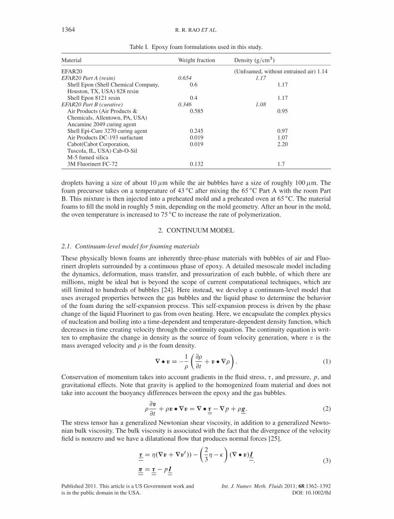
Table I. Epoxy foam formulations used in this study.
Material Weight fraction Density .g=cm3/
EFAR20 (Unfoamed, without entrained air) 1.14EFAR20 Part A (resin) 0.654 1.17
Shell Epon (Shell Chemical Company, 0.6 1.17Houston, TX, USA) 828 resinShell Epon 8121 resin 0.4 1.17
EFAR20 Part B (curative) 0.346 1.08Air Products (Air Products & 0.585 0.95Chemicals, Allentown, PA, USA)Ancamine 2049 curing agentShell Epi-Cure 3270 curing agent 0.245 0.97Air Products DC-193 surfactant 0.019 1.07Cabot(Cabot Corporation, 0.019 2.20Tuscola, IL, USA) Cab-O-SilM-5 fumed silica3M Fluorinert FC-72 0.132 1.7
droplets having a size of about 10�m while the air bubbles have a size of roughly 100�m. Thefoam precursor takes on a temperature of 43 ıC after mixing the 65 ıC Part A with the room PartB. This mixture is then injected into a preheated mold and a preheated oven at 65 ıC. The materialfoams to fill the mold in roughly 5 min, depending on the mold geometry. After an hour in the mold,the oven temperature is increased to 75 ıC to increase the rate of polymerization.
2. CONTINUUM MODEL
2.1. Continuum-level model for foaming materials
These physically blown foams are inherently three-phase materials with bubbles of air and Fluo-rinert droplets surrounded by a continuous phase of epoxy. A detailed mesoscale model includingthe dynamics, deformation, mass transfer, and pressurization of each bubble, of which there aremillions, might be ideal but is beyond the scope of current computational techniques, which arestill limited to hundreds of bubbles [24]. Here instead, we develop a continuum-level model thatuses averaged properties between the gas bubbles and the liquid phase to determine the behaviorof the foam during the self-expansion process. This self-expansion process is driven by the phasechange of the liquid Fluorinert to gas from oven heating. Here, we encapsulate the complex physicsof nucleation and boiling into a time-dependent and temperature-dependent density function, whichdecreases in time creating velocity through the continuity equation. The continuity equation is writ-ten to emphasize the change in density as the source of foam velocity generation, where v is themass averaged velocity and � is the foam density.
r � vD�1
�
�@�
@tC v �r�
�. (1)
Conservation of momentum takes into account gradients in the fluid stress, � , and pressure, p, andgravitational effects. Note that gravity is applied to the homogenized foam material and does nottake into account the buoyancy differences between the epoxy and the gas bubbles.
�@v
@tC �v �rvD r � � �rpC �g. (2)
The stress tensor has a generalized Newtonian shear viscosity, in addition to a generalized Newto-nian bulk viscosity. The bulk viscosity is associated with the fact that the divergence of the velocityfield is nonzero and we have a dilatational flow that produces normal forces [25].
� D �.rvCrvt //�
�2
3�� �
�.r � v/I
� D � � pI
. (3)
Published 2011. This article is a US Government work andis in the public domain in the USA.
Int. J. Numer. Meth. Fluids 2011; 68:1362–1392DOI: 10.1002/fld
A LEVEL SET METHOD TO STUDY FOAM PROCESSING: A VALIDATION STUDY 1365
It is a useful construct to define a total stress, �, based on the fluid stress and the pressure, as we will
see in subsequent sections. The generalized Newtonian viscosity models imply that the viscosities� and � vary with local fields, but still have a Newtonian form where stress is proportional to strain.However, the gradients of � and � are nonzero and must be included in the momentum equation.Here, both the shear and bulk viscosities are a function of temperature, degree of polymerization,and gas bubble volume fraction, which is related to the foam density (see Subsection 2.2.4). Oncethe stress tensor is substituted into the momentum equation, we obtain the usual Newtonian termsplus the bulk viscosity and gradients of the viscosity model.
Because the process is nonisothermal, heat transfer effects must be followed as well. The energyequation has a variable heat capacity, Cp , and thermal conductivity, k, both of which depend on thegas volume fraction. Heat is generated by the exothermic polymerization reaction and is depletedvia the evaporation of Fluorinert.
�Cp@T
@tC �Cpv �rT D r � .krT /C SrxnC Sevap (4)
Here, we ignore the effect of Fluorinert evaporation because it is a small effect compared withoven heating and exothermicity. Heat produced from the exothermic polymerization reaction of theepoxy-amine is tracked
Srxn D�Hrxn�Yo
ed�
dt, (5)
where Y oe is the initial mass fraction of epoxy prepolymer and � is the extent of reaction. The epoxypolymerization follows condensation chemistry, where the complex kinetics can be represented bythe extent of reaction � [19]. The extent of reaction is calculated from the following equation, whichincludes its time evolution, advection, and reaction kinetics:
@�
@tC v �r� D kieEa=RT .AC �m/.1� �/n. (6)
Material models to populate the conservation equations were determined from experimental mea-surements and literature review, as discussed in the next section. More details of the experimentsand experimental methods can be found in a report by Mondy et al. [23].
2.2. Material models for continuum equations
In this section, we discuss the material models used to populate the continuum conservationequations discussed in the previous section. Here we summarize our variable density models, curekinetics, complex viscosity and thermal properties.
2.2.1. Variable density models. From foam rise rate experiments, we can determine a time-dependent density function. Details of these experiments can be found elsewhere [23]. Followingthe idea of Seo et al. [2] to encapsulate foam nucleation and growth into a simple time-dependentdensity model with no spatial variations, we extend their model to include temperature dependence.Within the range of the temperatures tested, as the temperature increases, the foam rises faster. Here,we use the form suggested by Seo et al. [2], but use temperature-dependent parameters found fromempirical data,
�D .�initial � �final/ exp
��t
C.T /
�C �final
where C.T /DA
T�B
, (7)
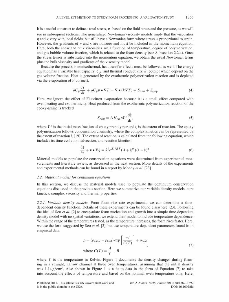
where T is the temperature in Kelvin. Figure 1 documents the density changes during foam-ing in a straight, narrow channel at three oven temperatures, assuming that the initial densitywas 1.14 g=cm3. Also shown in Figure 1 is a fit to data in the form of Equation (7) to takeinto account the effects of temperature and based on the nominal oven temperature only. Here,
Published 2011. This article is a US Government work andis in the public domain in the USA.
Int. J. Numer. Meth. Fluids 2011; 68:1362–1392DOI: 10.1002/fld

1366 R. R. RAO ET AL.
Figure 1. Foam density evolution as measured in original experiments at various temperatures, comparedwith Equation (7) with C.T /D A=T �B .
�final was taken to be 0.27 g=cm3, the value typically measured in this series of experiments.Fitting Equation (7) to the data in Figure 1 resulted in values for the parameters, A and B ,of 116,250 s and 274.26 s, respectively, yielding time constants for the exponential change in thefoam density of 69.5 s at 65 ıC and 7.1 s at 140 ıC. The model must be populated through specificexperiments, for each foam studied, to obtain coefficients A and B . Thus, it is an empirical model.However, if a different foam formulation is used, a reasonable model is obtained by using the initialand final density of the foam in the equation with a curve fit for C at the desired temperature. TheEFAR foam cannot be preheated to the oven temperature because that would boil the Fluorinert pre-maturely. The experiments for fitting the density function do involve a ramp of the temperature fromthe mixing/injection temperature, but this ramp was designed to be similar, if not identical, to thatoccurring in the validation experiment and the real applications. The mixing temperature is 43 ıC,and during injection through lines in the hot oven (at 65 ıC) into the preheated mold the prefoamedmaterial obtains an initial temperature of about 53 ıC before heating up to the oven temperature asit foams, as will be demonstrated in the results section.
2.2.2. Epoxy polymerization model. The reaction kinetics were measured with a TA Instruments(New Castle, DE, USA) Q200 differential scanning calorimeter. From these data, one can determinethe heat of reaction associated with the polymerization, the extent of reaction, and the derivativeof extent of reaction with time. With the extent of reaction and the reaction rate, in addition tothe assumption that the epoxy follows condensation chemistry [26], we can populate the parame-ters in Equation (6) and determine a kinetic rate model [35]. Figure 2 gives a comparison of theexperimental rate and extent of reaction to the modeled fits to the data.
The parameter values for the epoxy polymerization kinetics are also summarized in Table II.This detailed model of the polymerization reaction can be used to determine a curing viscosity
model as discussed in the following section.
2.2.3. Viscosity models. Foam rheological properties are complex measurements to perform in areproducible manner, because shearing the foam often changes the microstructure thereby alteringthe viscosity. For this reason, we decided to separate the viscosity into two parts dependent on: (1)continuous phase epoxy properties, extent of reaction and temperature and (2) gas bubble volumefraction. We assume these components are multiplicative because these effects are separable andcan be decoupled. (Note that the effect of Fluorinert droplets on the viscosity is ignored because itis a secondary effect). This assumption is based on the suspension/emulsion literature, which hasclearly shown that the effects of the continuous phase are separable from the discontinuous particle,
Published 2011. This article is a US Government work andis in the public domain in the USA.
Int. J. Numer. Meth. Fluids 2011; 68:1362–1392DOI: 10.1002/fld

A LEVEL SET METHOD TO STUDY FOAM PROCESSING: A VALIDATION STUDY 1367
Figure 2. Experimental data compared with curve fits of the extent of reaction (left) and the reaction rate,d=dt (right).
Table II. Epoxy polymerization kinetic parameters.
Epoxy cure parameter Value
Rate coefficient, ki 8.6� 103 1=sActivation energy, Ea 11 kcal/molRate parameter, A 0Rate exponent, m 0Rate exponent, n 1.4Heat of reaction, �Hrxn 250 J/g
emulsion, or gas bubble phases [27, 28].
�D �epoxy�� (8)
For the first term, rheological measurements were made for the continuous phase epoxy monomer,without Fluorinert, as a function of time as it polymerized in a Rheometrics ARES rheometerwith parallel plate geometry at a steady shear rate of 2 s�1. Various isothermal experiments wereundertaken at seven temperatures ranging from room temperature to 95 ıC.
The experimental data are shown in Figure 3.For operating temperatures far above the current glass transition temperature of the reacting
epoxy, the temperature dependence can be modeled accurately by an Arrhenius relationship [29].
Figure 3. Viscosity prediction for the continuous phase viscosity, without foaming.
Published 2011. This article is a US Government work andis in the public domain in the USA.
Int. J. Numer. Meth. Fluids 2011; 68:1362–1392DOI: 10.1002/fld

1368 R. R. RAO ET AL.
Dynamic percolation theory predicts a dependence of the Newtonian viscosity on extent of reactionwith the form
�epoxy D �00 exp
�Ea
RT
� �bc � �
b
�bc
!p(9)
where �c is the extent of reaction at the gel point, Ea is the activation energy, and �00 is the uncuredviscosity at reference temperature T0, and b and p are exponents for the model, with b being posi-tive and p being negative [30]. Note, also shown in Figure 3 is the curing viscosity model fit fromEquation (9). The parameters to populate this model are given in Table III.
We expected the foam viscosity �� to be a strong function of the gas volume fraction g and to fol-low the Taylor–Mooney form derived from emulsion experiments, extrapolating the discontinuousphase viscosity to zero [28]
�� D �0 exp
�g
1� g
�. (10)
To determine if this was a satisfactory approximation of the foam effective viscosity, we tested ourepoxy foam as it was expanding in a shear rheometer using the parallel plate geometry. Because thefoam was expanding during the test, the foam escaped out the side of the parallel plates and there-fore the volume of the sample did not change, but the density of the sample did. Both quantitiesare needed for the interpretation of the viscosity measurement. We used a temperature ramp in therheometer that mimicked that of the free-rise experiments. Knowing that the viscosity of the foamwould be sensitive to cell breakage, we tested a shear rate as low as possible given the resolution ofthe torque sensor in the rheometer. We assumed that the shear rate in the geometries of most inter-est, under the conditions of self expansion, would indeed be very low. The gas fraction (density) ateach moment in time was estimated from free-rise tests. The measured viscosity of the foam wascompared with that predicted by Equation (10) and found to be adequate (Figure 4) for low shearrates. The comparison is reasonable to a gas fraction greater than 0.6, while the expected limit ofthis equation is a gas fraction of 0.5 [28].
The total shear viscosity model, including the effects of curing epoxy and gas bubbles issummarized in the equation below
�foam D �00 exp
�Ea
RT
� �bc � �
b
�bc
!pexp
�g
1� g
�. (11)
To determine the foam stress tensor, we must understand both the shear and bulk viscosity. Follow-ing Batchelor [31], for the simple system of an incompressible liquid with a population of com-pressible bubbles, expansion occurs solely through the increase in the size of the bubbles while flowoccurs around each bubble. The effective expansion viscosity may be determined by equating thetotal dissipation as it would appear for a homogeneous fluid to the total dissipation from the ordinaryshear viscosity in the liquid surrounding the bubbles. Doing these calculations yields the result
� D4
3
�epoxy
g. (12)
Table III. Curing epoxy viscosity model parameters.
Curing epoxy viscosity model parameter Value
Uncured viscosity, at reference T , �00 4.0� 10�9 Pa sActivation energy, Ea 13 kcal/molExtent of reaction at gel point, �c 0.6Curing viscosity exponent, p �3.5Curing viscosity exponent, b 1.0
Published 2011. This article is a US Government work andis in the public domain in the USA.
Int. J. Numer. Meth. Fluids 2011; 68:1362–1392DOI: 10.1002/fld

A LEVEL SET METHOD TO STUDY FOAM PROCESSING: A VALIDATION STUDY 1369
Figure 4. Foam viscosity experiments (blue) plotted with Taylor–Mooney theoretical viscosity model (pink)for foam viscosity as a function of gas volume fraction.
Equation (12) may be extended to nondilute conditions, which was performed by Kraynik et al.[32] who used two-dimensional boundary integral calculations and three-dimensional ALE-freesurface calculations of expansion in a Kelvin cell. Their numerical results demonstrated thefollowing formula:
� D4
3�epoxy
.1� g/
g. (13)
We should note in any case that the Equation (13) results are the most pertinent because theyinvolve processes where the divergence of velocity is large. As g ! 0 the liquid becomes increas-ingly incompressible, the velocity becomes solenoidal .r � vD 0/, and bulk viscosity is no longerimportant.
2.2.4. Gas production model. The gas volume fraction, necessary for the viscosity and thermalmodels, can be determined from post-processing the density model and knowing some of the purecomponent mass fractions and densities
g D1� �
�i
1��ov�ol
C�Ya
�oa(14)
where �i is the initial precursor foam density, �0v is the density of pure Fluorinert vapor, �0l is thedensity of pure Fluorinert liquid, Ya is the mass fraction of air, and �0a is the density of pure air. Thevalues used for calculating the volume fraction of gas are summarized in Table IV.
Table IV. Parameters for gas evolution model.
Gas evolution parameter Value
Density of initial foam precursor, �i 1.14 g=cm3
Density of fluorinert liquid, 1.68 g=cm3
Density of fluorinert vapor, 0.0139 g=cm3
Mass fraction air, Ya 0–2.6e-4
Published 2011. This article is a US Government work andis in the public domain in the USA.
Int. J. Numer. Meth. Fluids 2011; 68:1362–1392DOI: 10.1002/fld

1370 R. R. RAO ET AL.
2.2.5. Thermal properties model. Foam heat capacity and thermal conductivity are strong func-tions of gas volume fraction and necessary for the energy equation, Equation (4). From Gibson andAshby [33], the foam heat capacity can be calculated from mixture theory for a two-phase materialof epoxy and gas bubbles
Cp DOcp,l�l.1� g/C Ocp,g�gg
�(15)
Here, Ocp,l is the heat capacity of the continuous liquid phase and Ocp,g is the heat capacity of the gasphase, �l is the density of the liquid phase and �g is the density of the gas phase.
An upper limit for the thermal conductivity of the foam mixture is given by the followingequation [34]:
k D2=3g kgC kl
�1�
2=3g
��2=3g � g
�kg
klC�1�
2=3g C g
� C kr. (16)
This equation stems from an analysis of conduction through a solid matrix with cubic bubblesarranged in line where kg is the gas conductivity, kl is the liquid phase conductivity, and kr is theheat conduction from radiation. In our initial implementation, we ignore any radiative contributionsassuming that at an oven temperature of 65 ıC, they will not be important. This can be tested whenwe undertake our thermal validation and compare this model to experimental data. Liquid phaseproperties were estimated by direct measurement, namely, density, and from experience with othersimilar epoxy systems [35]. Gas phase properties were estimated from air properties.
The summary of the parameters used in the thermal models is given in Table V. The initial massfractions of epoxy and air can be found in Tables I and IV.
3. NUMERICAL METHOD
The SIERRA (Sandia National Laboratories, Albuquerque, NM, USA) mechanics framework isbased on the FEM and designed to solve the equations of motion for both fluid and solid mechan-ics and has been chosen as the nuclear weapon’s tri-laboratory engineering analysis code [36].SIERRA/ARIA (Sandia National Laboratories, Albuquerque, NM, USA) was originally developedfor modeling low speed flows for applications such as manufacturing, focusing on incompress-ible flows [37]. Free surface flows, using both Eulerian and Lagrangian methods, were also afocus. ARIA was chosen as the development platform for foam encapsulation modeling becauseit had performed well for other similar free surface flows such as injection molding [38] and epoxyencapsulation [39].
3.1. Interface tracking via the level set method
As the foam expands via Fluorinert nucleation and growth, the material slowly fills the mold. Thelocation of the foam–air interface must be determined from the complex interplay of density evo-lution, velocity generation, viscous stress, surface tension, and gravitational effects, and it must bedetermined as part of the solution method. Many methods are available to determine the location of
Table V. Thermal model parameters.
Thermal model parameters Value
Heat capacity of liquid phase 2.0 J/gKHeat capacity of gas phase 1.0 J/gKDensity of liquid phase, �l 1.14 g=cm3
Density of gas phase, �g 0.001 g=cm3
Thermal conductivity of liquid phase, kl 0.18 W/mKThermal conductivity of liquid phase, kg 0.025 W/mKHeat of vaporization, Fluorinert, � OHevap 87.1 J/g
Published 2011. This article is a US Government work andis in the public domain in the USA.
Int. J. Numer. Meth. Fluids 2011; 68:1362–1392DOI: 10.1002/fld
A LEVEL SET METHOD TO STUDY FOAM PROCESSING: A VALIDATION STUDY 1371
the free surface from moving mesh methods to volume of fluid methods. Here, we use an Eulerianapproach based on a diffuse interface implementation of the level set method [14]. Because it isan Eulerian approach it can handle geometric complexity and topological changes, such as dropletbreakup, without complex remeshing and remapping steps.
The level set, .x,y, ´, t /, is a signed distance function of space and time. The magnitude of thelevel set function is the shortest distance from x to any point on the free surface, where the freesurface is defined by the level set zero. The sign of level set is used to indicate whether the pointx lies inside the material. It should be noted that should scale as a distance function, that is, themagnitude of its gradient is unity
jrj D 1. (17)
This level set representation of the interface presents numerous advantages. The location of theinterfacial curve can be determined exactly from interpolation of the finite element shape functions.In addition, the level set representing function provides immediate information about the normal,nls, and curvature, H, of the interfacial surface via these relations
nls Dr
jrj
HD�r2
jrj
. (18)
Because the level set zero,
.x,y, ´, t /D 0 (19)
is a material surface, it advects with the fluid velocity, whereas elsewhere it is unclear how the levelset equation evolves. For this reason, we use an advection equation for the entire level set function.
@
@tC u �r D 0. (20)
Because advection is only truly applicable at the interface, Equation (20) distorts the distance func-tion. This necessitates the use of a renormalizing algorithm, which must be run periodically tocorrect the distance function. Here, we utilize a constrained redistancing algorithm that attemptsto redistance the level set so that the volume of each phase remains unchanged. Details of therenormalization algorithm can be found below.
3.1.1. Property evaluation and equation averaging. Notationally, we denote these two sides of theinterface as ‘phase A’ and ‘phase B’ and often use ‘A’ and ‘B’ as subscripts on mathematical quanti-ties that are specific to a phase. By convention, we associate phase A with the negative level set fieldand B with the positive phase. The level set method uses continuous equations for both the foam andgas phase, but modulates the material properties based on the level set function. This property mod-ulation occurs via a numerical Heaviside function defined for phase A and B, where the Heavisidefunctions sum to one
HA./CHB./D 1. (21)
In the diffuse interface approach, the Heaviside function is regularized so that there is a smoothtransition from one phase to another. In this work, we use
HB./D1
2
0BB@1C
2C
sin
��
˛
��
1CCA ,�˛ < < ˛, (22)
Published 2011. This article is a US Government work andis in the public domain in the USA.
Int. J. Numer. Meth. Fluids 2011; 68:1362–1392DOI: 10.1002/fld

1372 R. R. RAO ET AL.
where ˛ is defined as half of the width of the diffuse interface, which is usually taken as about sixelements across. Here, HB is zero in phase A, 1 in phase B, and follows Equation (22) in the dif-fuse region. Another useful function related to the Heaviside function is the regularized Dirac deltafunction, which is defined as
ı˛./DdH./
dDjj
2˛
�1C cos
��
˛
��,�˛ < < ˛, (23)
where ı˛./ is large in the diffuse interface zone and zero elsewhere.We use an equation averaging technique to modulate between the properties in each phase. The
continuity equation, (1), can be rewritten including the Heaviside function to modulate the densityfrom foam to gas phase.
.HA�ACHB�B/r � vD�HA
�@�A
@tC v �r�A
��HB
�@�B
@tC v �r�B
�. (24)
Assuming here that the foam phase is designated A and the gas phase designated B, we assume thefoam has a variable density and ignore any density variations in the air phase because their variationswill be orders of smaller magnitude. This yields
.HA�ACHB�B/r � vD�HA
�@�A
@tC v �r�A
�. (25)
The momentum equation, (2), including property modulation, becomes
.HA�ACHB�B/
�@v
@tC v �rv
�DHAr � �ACHBr � �BC .HA�ACHB�B/g, (26)
where the phase-defined stress tensor is more complex for the foam, while the gas is assumed tohave a constant viscosity and be incompressible.
�A D �A � pAI
�B D �B � pBI(27)
The energy equation, (5), becomes
.HA�ACpACHB�BCpB/
�@T
@tC v �rT
�D r �..HAkACHBkB/rT /CHASrxnCHASevap (28)
with the heat source terms only occurring in the foam phase.The epoxy polymerization equation is also phase dependent and only has a nonzero right-hand
side source term in the foam phase.
3.1.2. Surface tension. Mold filling flows are often highly influenced by the capillary dynamicsat the fluid–gas interface, although it is unclear how important surface forces are to macroscopicfoam self-expansion flows. (On the microscopic level, surface forces are critical to understandingbubble expansion. However, gas evolution tends to drive the kinematics of foam filling.) Because ofthe implicit tracking of this interface, special care must be taken to enforce the capillary boundarycondition. The general form of the capillary boundary condition for constant surface tension, � , is
n � .�A� �
B/D�2H �n. (29)
Here, n is the unit normal along the exterior boundary of the domain. The value used for the surfacetension is that of the neat resin, as we assume that there is a resin-rich layer of fluid at the freesurface. For our epoxy polymer, we measure a surface tension of 39.8 dyne/cm.
Integrated boundary conditions, such as Equation (29), can be applied with the level set methodusing several techniques [40,41], only one of which we discuss here. To evaluate Equation (29), wemust construct a local mean curvature H. The local mean curvature is defined as
�HD r � n� r � nls Dr2
jrj(30)
Published 2011. This article is a US Government work andis in the public domain in the USA.
Int. J. Numer. Meth. Fluids 2011; 68:1362–1392DOI: 10.1002/fld
A LEVEL SET METHOD TO STUDY FOAM PROCESSING: A VALIDATION STUDY 1373
Hence, the curvature is related to the second derivative of . Because we use the standard finiteelement discretization for , it is only C 0 continuous and can only be differentiated once. Thus, inthis work, we solve for an approximation to the curvature, Hp, using a least squares, lumped massprojection that is integrated by parts, creating a boundary term in addition to the volume integral.Z
V
NiH pdV D�ZV
Ni .r � nls/dV D�ZV
rNi � nlsdV CZS
Nin � nlsdS . (31)
To enforce a prescribed contact angle, D cos�1.n � nls/ one would include the boundary term in(31) and replace n � nls with cos . For the application described here, we weakly impose D 90ı,so this boundary contribution is not included.
Because there is no explicit interface at D 0, we utilize the diffuse Dirac delta function andthe volumetric projection for the curvature Hp to implement the capillary boundary condition,Equation (29), viz.
n � .�B � �A/D 2�ı˛./H pnls (32)
following the continuous surface force literature [41].
3.1.3. Redistancing algorithm. One distinct aspect of the level set method is that while the levelset function might initially have the smooth properties of a distance function, this is not necessarilypreserved by the evolution scheme. It is almost certainly the case that as evolution proceeds it willdeviate away from a purely distance function. Indeed, sharp gradients might occur at some pointsin the flow, while very shallow gradients occur in others. The former is bad because it leads to inac-curacies in the integration of Equation (20); the latter is bad because it inappropriately widens thethickness of the interfacial zone. A necessary aspect of any level set method therefore is a periodicneed to redistance or renormalize the level set function back to a distance function. Our decisionto renormalize is based upon monitoring the average gradient magnitude of the level function overthe interfacial zone. In general, this average gradient is only allowed to vary between 1.25 and 0.75.Outside of this range it will trigger a redistancing procedure.
There are several methods by which this can be done. Sussman and Fatemi [42] described aredistancing step based upon a separate evolution of the level set field subject to a mass conservingconstraint. We have implemented a more algorithmic approach. The elements that contain the inter-face can be quickly identified as those whose nodal level set values have differing signs. On theseelements, a piecewise linear representation of the interface is constructed. For each node i in themesh, it is possible to find a minimum distanceDi to this set of facets. Renormalization of the levelset nodal unknown is made by the simple assignment
�j D sign�0jDj , (33)
where 0i is the value of the level set function prior to renormalization. Given a sufficient densityof facets, this procedure will yield good results and be fast and robust. However, it does present thepotential for slight, systemic motion of the zero level set contour and a consequent loss of mass.This is especially a problem for lower order (trilinear) interpolation of the level set function. Thiscan be avoided, however, by introducing a volume constraint. This is accomplished by finding asmall change to the distance function, ", such that the initial and final volumes are the same. Thedistance function at the end of the renormalization is thus given by
j D �j C " (34)
where " is found by solving the equationZV
H 0A.
�C "/dV DZV
H 0A.
0/dV . (35)
Published 2011. This article is a US Government work andis in the public domain in the USA.
Int. J. Numer. Meth. Fluids 2011; 68:1362–1392DOI: 10.1002/fld

1374 R. R. RAO ET AL.
The superscript on the Heaviside is used here to denote that this is the sharp Heaviside function,that is, unity where its argument is positive and zero elsewhere. The left-hand side of this equationis the volume of the phase A following the renormalization and the right-hand side is the volumebefore renormalization. By using this adjustment to the nearest point distance, we guarantee that thevolume of the phase A after renormalization will be the same as it was before renormalization.
3.2. Finite element discretization
The phase modulated equations of motion, conservation of energy, and kinetics equation, (25–28),together with the level set equation, (20), are discretized with the well-known Galerkin FEM. Fordetails of the FEM, see for instance Hughes [43]. The unknowns of interest are the velocity vector,pressure, temperature, extent of reaction, and level set. These fields are approximated with finiteelement basis function, Ni .x,y, ´/, and nodal variables, for example, ui , vi , wi , Ti , �i , i . BilinearLagrangian, C 0-continuous, basis functions are used for all variables. The velocity vector would beexpressed in the following manner:
uD
nXiD1
uiNi .x,y, ´/, vDnXiD1
viNi .x,y, ´/, w DnXiD1
wiNi .x,y, ´/ (36)
and pressure, temperature, extent of reaction, and level set are
p D
nXiD1
piNi .x,y, ´/, T DnXiD1
TiNi .x,y, ´/, � DnXiD1
�iNi .x,y, ´/, DnXiD1
iNi .x,y, ´/.
(37)
The approximate variables are substituted in the conservation equation, multiplied by a weightingfunction, and integrated over the domain. In the Galerkin FEM, the weight function is chosen tobe the bilinear shape functions themselves. Any second derivatives, such as the divergence of thestress tensor and the heat flux, are integrated by parts to improve the accuracy of the discretization asshown below. The integration by parts on the momentum and energy equations create surface termsthat serve as natural boundary conditions if no other conditions are applied at the domain bound-aries. (To make it easier to understand, we omit the Heaviside operation for equation averagingdiscussed in the previous section.)
Rcontinuityi D
ZV
Ni
��r � vC
�@�
@tC v �r�
��dV D 0, (38)
Rmomentumi D
ZV
�Ni
��@v
@tC �v �rv� �g
��r.eNi / W �
�dV C
ZS
n � � � eNidS D 0, (39)
Renergyi D
ZV
�Ni
��Cp
@T
@tC �Cpv �rT� Srxn � Sevap
��rNi � krT
�dV C
ZS
n�krT dS D 0,
(40)
Rcurei D
ZV
Ni
�@�
@tC v �r� � kieEa=RT .AC �m/.1� �/n
�dV D 0, (41)
Rlevelseti D
ZV
Ni
�@
@tC v �r
�dV D 0. (42)
Time derivative is discretized using a first-order backward Euler finite difference method. Theresulting weighted residual equations are integrated numerically using Gaussian quadrature.
Published 2011. This article is a US Government work andis in the public domain in the USA.
Int. J. Numer. Meth. Fluids 2011; 68:1362–1392DOI: 10.1002/fld

A LEVEL SET METHOD TO STUDY FOAM PROCESSING: A VALIDATION STUDY 1375
There exists an inf–sup condition constraining the pressure space to be one order lower than thevelocity space, which is termed the Ladyshenskaya-Babuska-Brezzi (LBB) condition [43]. To allowus to use equal order interpolation and circumvent the LBB condition, we must use a stabilizationmethod, an extra benefit of which is allowing us to use Krylov-based iterative solvers in place ofdirect solution methods. Details of the stabilization method used here are discussed in the followingsection.
3.2.1. Pressure stabilization. To circumvent the LBB condition, one must either use a compatiblepair of finite element basis functions between the velocity and pressure space or add stabilizationterms to relieve the mathematical restrictions. Many types of stabilization exist, the most commonbeing Galerkin least squares or pressure stabilized Petrov–Galerkin popularized by Hughes [43].These methods work well for moderate to high Reynolds’ number applications but have issues atthe Stokes limit. Other complexities arise relating to the scaling of the stabilization term and manypapers have been written trying to determine the best scaling coefficient.
Here, we employ the stabilization technique developed by Dohrmann and Bochev [22], which wasdeveloped for the Stokes problem and is termed pressure-stabilized pressure projection. In additionto being computationally efficient and easy to implement, this stabilization method is also easy touse because it requires no special treatment for boundary conditions. Numerically, this method sim-ply requires an additional volume integral term in the weak form of the continuity equation. Scalingof the stabilization term relies on dimensional analysis and does not contain an explicit mesh scal-ing. The first term is the standard Galerkin continuity-weighted residual, while the second term isthe stabilization.
Rcontinuityi D
ZV
Ni
��r � vC
�@�
@tC v �r�
��dV C
MXelem
�pspp.Ni �LNi /.p �Lp/dV
Lp D
ZVe
pdV=ZVe
dV
. (43)
For multiphase level set problems, there exists a pressure jump at the fluid–gas interface because ofsurface forces. Because we are applying a stabilization method developed for a single phase problemto a multiphase one, we have made a slight modification to the stabilization method that allows us tocapture the pressure jump at the fluid–gas interface. Instead of stabilizing on the pressure variable,we stabilize on the product of the time derivative of the pressure and the time step size as shownbelow
Rci D
ZV
Ni
�r � vC
1
�
�@p
@tC v �r�
��dV C
MXelem
�pspp�t.Ni �LNi /
�@p
@t�L
@p
@t
�dV
L@p
@tD
ZVe
@p
@tdV=
ZVe
dV
.
(44)This method has shown itself superior for mass conservation in level set problems compared withEquation (43) either with a single or dual pressure formulation [49].
3.2.2. Taylor–Galerkin upwinding for level set equation. The level set equation is purely hyper-bolic, whereas the Galerkin finite element works most effectively on elliptic differential equations.For that reason, we apply a Taylor–Galerkin upwinding term [44] to the level set equation to helpit behave well away from the interface. In the Taylor–Galerkin weighted residual of the level setadvection in Equation (20), the first two terms are the standard weighted residual advection operator,while the third term is the upwinding term.ZV
Ni
�nC1i � ni
�t
dV D�ZV
Ni�vnC1 �rnC1i
dV �
�t
2
ZV
.vn �rNi /�vn �rni
dV . (45)
Published 2011. This article is a US Government work andis in the public domain in the USA.
Int. J. Numer. Meth. Fluids 2011; 68:1362–1392DOI: 10.1002/fld

1376 R. R. RAO ET AL.
Because the magnitude of the gradient of the level set function is by definition a nearly constantvalue, the Taylor–Galerkin contribution is relatively small. This points to one of the advantages ofusing a smooth function to represent the interface location.
3.2.3. Streamline upwind Petrov–Galerkin for the momentum equation. As we move from theStokes’ regime to a moderate Reynolds’ number, we find that the differential equation changesfrom purely elliptic to hyperbolic-elliptic and some stabilization method is useful for the momen-tum equation. As the foam displaces the gas in the mold, the gas phase velocity increases resultingin a Reynolds’ number in the 10–100 range. This can trigger numerical issues such as oscillationsin the solution. We have found that adding some streamline upwinding Petrov–Galerkin (SUPG)improves the performance of the momentum equations and reduces oscillations in the pressure andvelocity. The SUPG method involves a modified weight function, Wi , consisting of the shape func-tion plus the velocity dotted into the gradient of the weight function multiplied by a scaling factorbased on element size.
Wi DNi C
MXelem
�SUPG.helem/v �rNi
jvj(46)
The weight function is applied only to the terms that are not integrated by parts, because a gradi-ent cannot be integrated by parts. This makes the SUPG method an inconsistent method for low tomoderate Reynolds’ numbers where the total stress dominates the residual. However, as the elementsize goes to zero it will asymptote to the correct partial differential equation
Rmomsupgi D
ZV
�Wi
��@v
@tC �v �rv� �g
��r.eNi / W �
�dV C
ZS
n � � � eNidS D 0. (47)
The SUPG primarily offers upwinding in the streamwise direction.
3.3. Matrix equations and Krylov-based iterative solvers
Once the residual equations are integrated, we obtain a set of nonlinear algebraic equations on eachelement that must be gathered into a global matrix and solved for the nodal unknowns. We solvethe level set equation in a separate matrix from the rest of the unknowns, because decoupling theequations seems to make the method more robust and improve convergence.
F.v,p,T , �/D 0
G./D 0. (48)
This system of equations is linearized and solved with the Newton–Raphson method, where F hasbeen expanded in a Taylor series about the kth iterate
F.v,p,T , �/C@F
@vjk.vkC1 � vk/C
@F
@pjk.pkC1 � pk/
C@F
@Tjk.T kC1 � T k/C
@F
@�jk.�kC1 � �k/D 0
@G
@jk.kC1 � k/D 0
. (49)
All the terms involving the kth iterate are gathered and placed on the right-hand side of the equation.This results in a matrix equation of the form
K.xk/�xkC1 D f , (50)
where K is an analytical Jacobian matrix and we solve for the unknown update from the last iter-ation, �xkC1. We have one matrix equation for the bulk fluid unknowns and one for the levelset unknowns.
Published 2011. This article is a US Government work andis in the public domain in the USA.
Int. J. Numer. Meth. Fluids 2011; 68:1362–1392DOI: 10.1002/fld

A LEVEL SET METHOD TO STUDY FOAM PROCESSING: A VALIDATION STUDY 1377
In two dimensions, we generally solve the fluid matrix equations with direct Gaussian elimina-tion, but in three dimensions, this becomes impossible because the matrix bandwidth is so muchlarger. Instead, we use Krylov-based iterative solvers from TRILINOS, an open source parallelsolver library developed at Sandia National Laboratories [45]. The stabilization of the continuityequation, Equation (44), has an additional benefit besides allowing equal order interpolants: it alsoadds a pressure term to the pressure equation, improving the diagonal dominance of the matrixequations (50), and reducing the matrix condition number. Needless to say, it would be near impos-sible to use iterative solvers on Equation (50) without stabilization. The discretized level set matrixequations, on the other hand, tend to be well-behaved as long as the velocity is well-behaved.
SIERRA/ARIA can be run in serial or parallel, where the parallel implementation is based ona message passing interface. For the problem discussed here, we focus on parallel solutions runon 68 processors on the Sandia National Laboratories capacity computing platform, Thunderbird.Each run on Thunderbird would take about 16–25 h, depending on the complexity of the physicsmodels used.
Parallel iterative solvers always require preconditioning. Some of the preconditioners suitable forlevel set foaming problems are ILU and ILUT, with fill factors of 1–3. Note that as we increase thefill factors, the time to solve the matrix equations increases sharply. Solvers used here range fromBiCGStab to GMRES. Generally, for the problems described here, we resort to ILUT(3)/GMRES,which is the most robust but also the most expensive choice.
3.4. Geometry, mesh, initial conditions and boundary conditions
A mold with a complex geometry has been developed to test foam quality. This quality assurance(QA) fixture developed at Kansas City Plant is pictured in Figure 5. For the QA fixture, a complexchannel is machined in an aluminum block and a clear acrylic cover is held on the front face withscrews. To monitor the quality of the foam during an encapsulation process, this mold is filled withthe foam encapsulant and monitored to make sure that it fills the part. Filling is through injectionports in the left hand corner of either the inner cup shape or the outer serpentine shape as shownin Figure 5. The mold was instrumented with four thermocouples. The first thermocouple, TC101,is in the injection port machined through the back wall. It is not quite in the main reservoir. Ther-mocouples TC102 and TC103 are in the foam channel as pictured, about halfway between the frontface of the back wall and the inner surface of the front cover and about halfway across the channelwidth. The fourth, TC104, is within the mold itself, centered in the aluminum block about 0.16 cm(1/16 in) from the inner face of the back wall, and so never touches foam.
The outer mold, consisting of narrow sections and serpentine routes for the foam to penetrate,was used for model validation studies. The inner cup was filled in the initial trials, but later ignored.
Figure 5. QA fixture (left), as seen in the videos and annotated (right).
Published 2011. This article is a US Government work andis in the public domain in the USA.
Int. J. Numer. Meth. Fluids 2011; 68:1362–1392DOI: 10.1002/fld
1378 R. R. RAO ET AL.
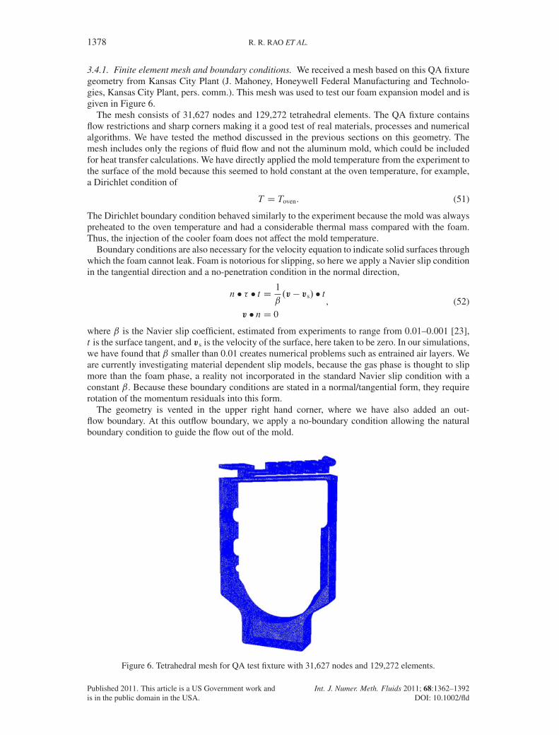
3.4.1. Finite element mesh and boundary conditions. We received a mesh based on this QA fixturegeometry from Kansas City Plant (J. Mahoney, Honeywell Federal Manufacturing and Technolo-gies, Kansas City Plant, pers. comm.). This mesh was used to test our foam expansion model and isgiven in Figure 6.
The mesh consists of 31,627 nodes and 129,272 tetrahedral elements. The QA fixture containsflow restrictions and sharp corners making it a good test of real materials, processes and numericalalgorithms. We have tested the method discussed in the previous sections on this geometry. Themesh includes only the regions of fluid flow and not the aluminum mold, which could be includedfor heat transfer calculations. We have directly applied the mold temperature from the experiment tothe surface of the mold because this seemed to hold constant at the oven temperature, for example,a Dirichlet condition of
T D Toven. (51)
The Dirichlet boundary condition behaved similarly to the experiment because the mold was alwayspreheated to the oven temperature and had a considerable thermal mass compared with the foam.Thus, the injection of the cooler foam does not affect the mold temperature.
Boundary conditions are also necessary for the velocity equation to indicate solid surfaces throughwhich the foam cannot leak. Foam is notorious for slipping, so here we apply a Navier slip conditionin the tangential direction and a no-penetration condition in the normal direction,
n � � � t D1
ˇ.v� vs/ � t
v � nD 0
, (52)
where ˇ is the Navier slip coefficient, estimated from experiments to range from 0.01–0.001 [23],t is the surface tangent, and vs is the velocity of the surface, here taken to be zero. In our simulations,we have found that ˇ smaller than 0.01 creates numerical problems such as entrained air layers. Weare currently investigating material dependent slip models, because the gas phase is thought to slipmore than the foam phase, a reality not incorporated in the standard Navier slip condition with aconstant ˇ. Because these boundary conditions are stated in a normal/tangential form, they requirerotation of the momentum residuals into this form.
The geometry is vented in the upper right hand corner, where we have also added an out-flow boundary. At this outflow boundary, we apply a no-boundary condition allowing the naturalboundary condition to guide the flow out of the mold.
Figure 6. Tetrahedral mesh for QA test fixture with 31,627 nodes and 129,272 elements.
Published 2011. This article is a US Government work andis in the public domain in the USA.
Int. J. Numer. Meth. Fluids 2011; 68:1362–1392DOI: 10.1002/fld
A LEVEL SET METHOD TO STUDY FOAM PROCESSING: A VALIDATION STUDY 1379
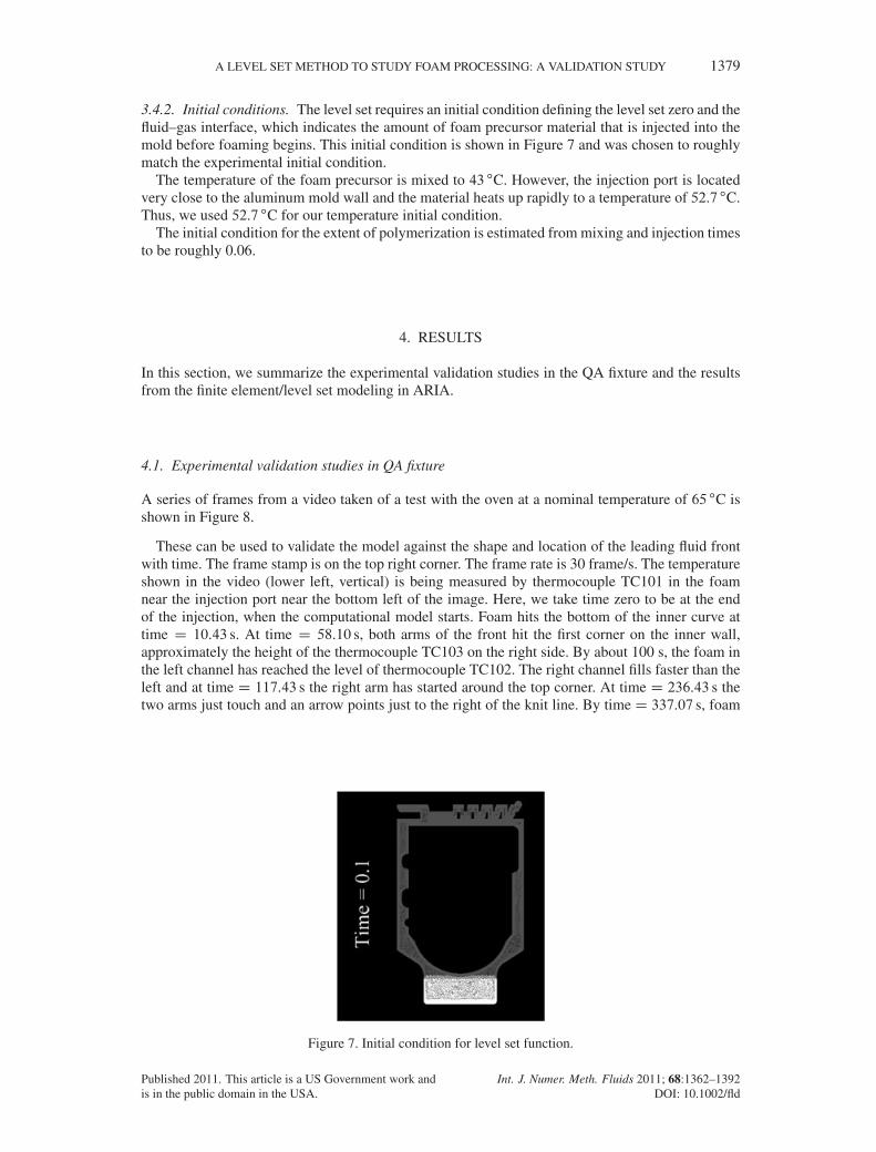
3.4.2. Initial conditions. The level set requires an initial condition defining the level set zero and thefluid–gas interface, which indicates the amount of foam precursor material that is injected into themold before foaming begins. This initial condition is shown in Figure 7 and was chosen to roughlymatch the experimental initial condition.
The temperature of the foam precursor is mixed to 43 ıC. However, the injection port is locatedvery close to the aluminum mold wall and the material heats up rapidly to a temperature of 52.7 ıC.Thus, we used 52.7 ıC for our temperature initial condition.
The initial condition for the extent of polymerization is estimated from mixing and injection timesto be roughly 0.06.
4. RESULTS
In this section, we summarize the experimental validation studies in the QA fixture and the resultsfrom the finite element/level set modeling in ARIA.
4.1. Experimental validation studies in QA fixture
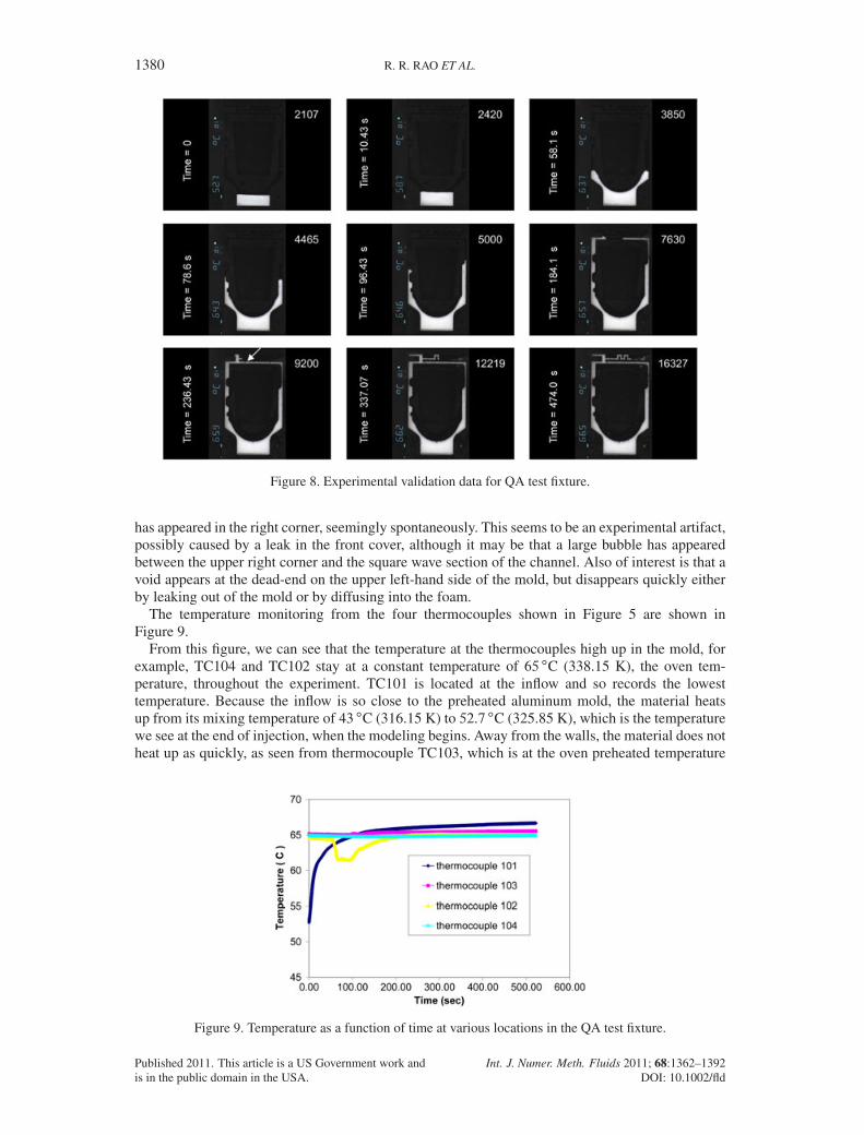
A series of frames from a video taken of a test with the oven at a nominal temperature of 65 ıC isshown in Figure 8.
These can be used to validate the model against the shape and location of the leading fluid frontwith time. The frame stamp is on the top right corner. The frame rate is 30 frame/s. The temperatureshown in the video (lower left, vertical) is being measured by thermocouple TC101 in the foamnear the injection port near the bottom left of the image. Here, we take time zero to be at the endof the injection, when the computational model starts. Foam hits the bottom of the inner curve attime D 10.43 s. At time D 58.10 s, both arms of the front hit the first corner on the inner wall,approximately the height of the thermocouple TC103 on the right side. By about 100 s, the foam inthe left channel has reached the level of thermocouple TC102. The right channel fills faster than theleft and at time D 117.43 s the right arm has started around the top corner. At time D 236.43 s thetwo arms just touch and an arrow points just to the right of the knit line. By time D 337.07 s, foam
Figure 7. Initial condition for level set function.
Published 2011. This article is a US Government work andis in the public domain in the USA.
Int. J. Numer. Meth. Fluids 2011; 68:1362–1392DOI: 10.1002/fld
1380 R. R. RAO ET AL.
Figure 8. Experimental validation data for QA test fixture.
has appeared in the right corner, seemingly spontaneously. This seems to be an experimental artifact,possibly caused by a leak in the front cover, although it may be that a large bubble has appearedbetween the upper right corner and the square wave section of the channel. Also of interest is that avoid appears at the dead-end on the upper left-hand side of the mold, but disappears quickly eitherby leaking out of the mold or by diffusing into the foam.
The temperature monitoring from the four thermocouples shown in Figure 5 are shown inFigure 9.
From this figure, we can see that the temperature at the thermocouples high up in the mold, forexample, TC104 and TC102 stay at a constant temperature of 65 ıC (338.15 K), the oven tem-perature, throughout the experiment. TC101 is located at the inflow and so records the lowesttemperature. Because the inflow is so close to the preheated aluminum mold, the material heatsup from its mixing temperature of 43 ıC (316.15 K) to 52.7 ıC (325.85 K), which is the temperaturewe see at the end of injection, when the modeling begins. Away from the walls, the material does notheat up as quickly, as seen from thermocouple TC103, which is at the oven preheated temperature
Figure 9. Temperature as a function of time at various locations in the QA test fixture.
Published 2011. This article is a US Government work andis in the public domain in the USA.
Int. J. Numer. Meth. Fluids 2011; 68:1362–1392DOI: 10.1002/fld
A LEVEL SET METHOD TO STUDY FOAM PROCESSING: A VALIDATION STUDY 1381
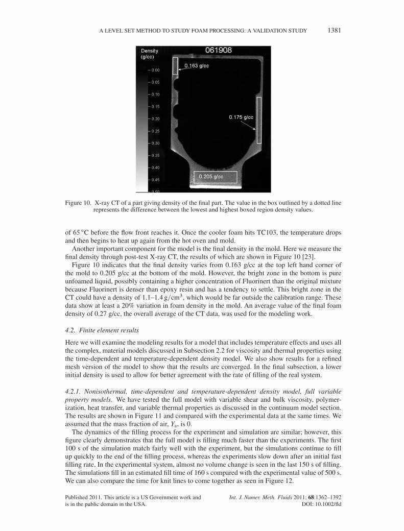
Figure 10. X-ray CT of a part giving density of the final part. The value in the box outlined by a dotted linerepresents the difference between the lowest and highest boxed region density values.
of 65 ıC before the flow front reaches it. Once the cooler foam hits TC103, the temperature dropsand then begins to heat up again from the hot oven and mold.
Another important component for the model is the final density in the mold. Here we measure thefinal density through post-test X-ray CT, the results of which are shown in Figure 10 [23].
Figure 10 indicates that the final density varies from 0.163 g/cc at the top left hand corner ofthe mold to 0.205 g/cc at the bottom of the mold. However, the bright zone in the bottom is pureunfoamed liquid, possibly containing a higher concentration of Fluorinert than the original mixturebecause Fluorinert is denser than epoxy resin and has a tendency to settle. This bright zone in theCT could have a density of 1.1–1.4 g=cm3, which would be far outside the calibration range. Thesedata show at least a 20% variation in foam density in the mold. An average value of the final foamdensity of 0.27 g/cc, the overall average of the CT data, was used for the modeling work.
4.2. Finite element results
Here we will examine the modeling results for a model that includes temperature effects and uses allthe complex, material models discussed in Subsection 2.2 for viscosity and thermal properties usingthe time-dependent and temperature-dependent density model. We also show results for a refinedmesh version of the model to show that the results are converged. In the final subsection, a lowerinitial density is used to allow for better agreement with the rate of filling of the real system.
4.2.1. Nonisothermal, time-dependent and temperature-dependent density model, full variableproperty models. We have tested the full model with variable shear and bulk viscosity, polymer-ization, heat transfer, and variable thermal properties as discussed in the continuum model section.The results are shown in Figure 11 and compared with the experimental data at the same times. Weassumed that the mass fraction of air, Ya, is 0.
The dynamics of the filling process for the experiment and simulation are similar; however, thisfigure clearly demonstrates that the full model is filling much faster than the experiments. The first100 s of the simulation match fairly well with the experiment, but the simulations continue to fillup quickly to the end of the filling process, whereas the experiments slow down after an initial fastfilling rate. In the experimental system, almost no volume change is seen in the last 150 s of filling.The simulations fill in an estimated fill time of 160 s compared with the experimental value of 500 s.We can also compare the time for knit lines to come together as seen in Figure 12.
Published 2011. This article is a US Government work andis in the public domain in the USA.
Int. J. Numer. Meth. Fluids 2011; 68:1362–1392DOI: 10.1002/fld

1382 R. R. RAO ET AL.
Figure 11. Comparison between simulation (top) and experiments (bottom) for the full model with variableproperties, heat transfer and polymerization.
Again, the knit lines are coming together much sooner for the simulation than the experiment andalso in different places. From viewing the movie and the stills, we find that there are several dis-crepancies between the experiment and the model. First, the upper right hand channel looks muchnarrower in the experiment, and because of the fineness of the channel we find single bubbles mov-ing although this part of the domain like red blood cells in a capillary. In other words, the bubblesare displaying noncontinuum effects not accounted for in our model where we need to have at least6–10 bubbles across the domain to assume a continuum.
Another issue that can affect the ARIA results is the choice of slip model and the value of theNavier slip coefficient. Using a Navier slip coefficient from PIV data [23] leads to an entrained gaslayer at the solid surfaces. However, we may be getting too much slip at the boundary and mayneed to investigate other wetting models. Other discrepancies between the model and the experi-ment occur in the density model itself and the choice of parameters to populate it, which will bediscussed in the following section.
As part of the study, we also wanted to check the convergence of the solution with mesh refine-ment. We took the fairly refined mesh given in Figure 6 and did a consistent mesh refinement,keeping the same topology and refining with the CUBIT mesh generation package [51]. This meshrefinement took every tetrahedral element and split it into eight tetrahedral elements. This resulted ina mesh with 916,512 nodes and 1,034,176 elements. The refined mesh solution ran for two months
Figure 12. Time and place where knit lines come together for ARIA simulations for full model and exper-imental flow visualization: the left is simulation at time D 132.1 s and right is data at time D 236.4 s. Red
arrows indicate the place where knit lines join in the mold.
Published 2011. This article is a US Government work andis in the public domain in the USA.
Int. J. Numer. Meth. Fluids 2011; 68:1362–1392DOI: 10.1002/fld
A LEVEL SET METHOD TO STUDY FOAM PROCESSING: A VALIDATION STUDY 1383
on all 64 processors of a shared memory cluster of eight multicore processors. Each processor is anIntel Xeon CPU running at 2.27 GHz.
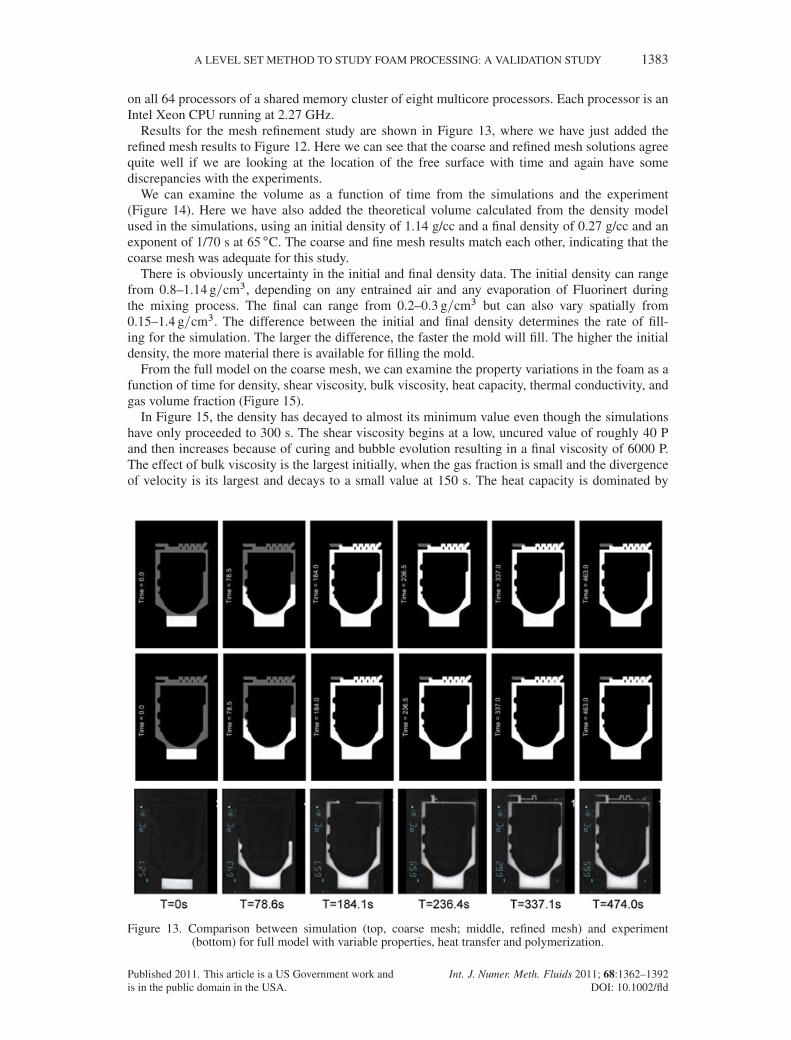
Results for the mesh refinement study are shown in Figure 13, where we have just added therefined mesh results to Figure 12. Here we can see that the coarse and refined mesh solutions agreequite well if we are looking at the location of the free surface with time and again have somediscrepancies with the experiments.
We can examine the volume as a function of time from the simulations and the experiment(Figure 14). Here we have also added the theoretical volume calculated from the density modelused in the simulations, using an initial density of 1.14 g/cc and a final density of 0.27 g/cc and anexponent of 1/70 s at 65 ıC. The coarse and fine mesh results match each other, indicating that thecoarse mesh was adequate for this study.
There is obviously uncertainty in the initial and final density data. The initial density can rangefrom 0.8–1.14 g=cm3, depending on any entrained air and any evaporation of Fluorinert duringthe mixing process. The final can range from 0.2–0.3 g=cm3 but can also vary spatially from0.15–1.4 g=cm3. The difference between the initial and final density determines the rate of fill-ing for the simulation. The larger the difference, the faster the mold will fill. The higher the initialdensity, the more material there is available for filling the mold.
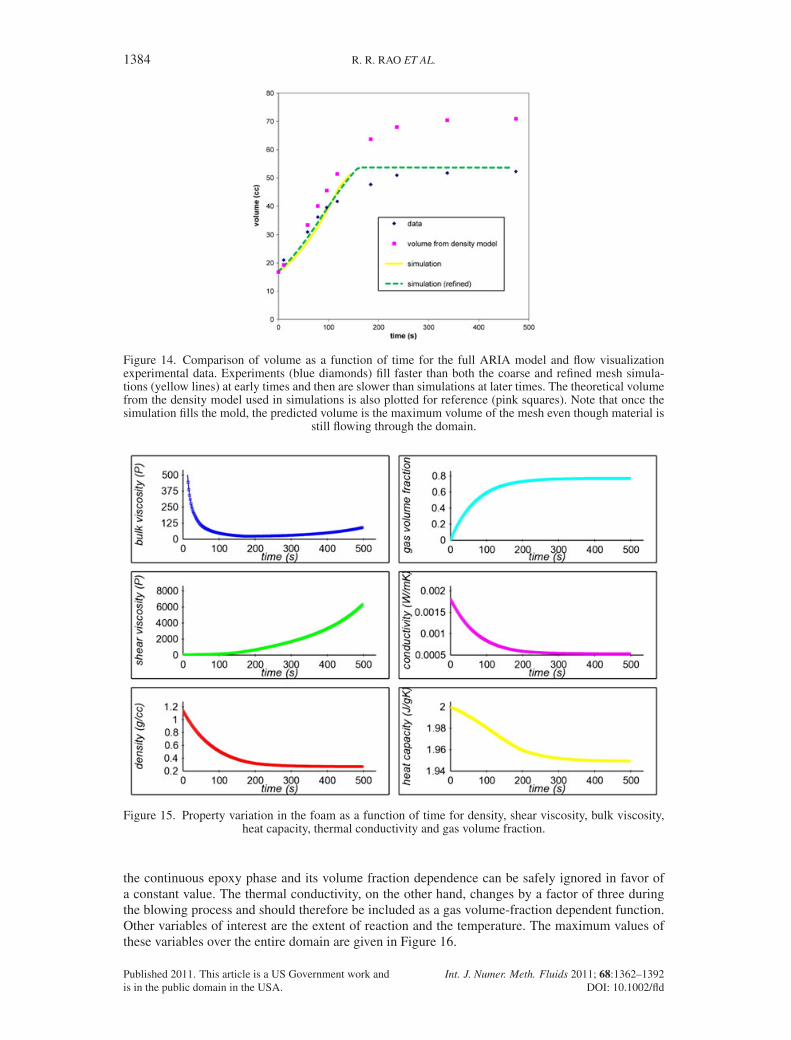
From the full model on the coarse mesh, we can examine the property variations in the foam as afunction of time for density, shear viscosity, bulk viscosity, heat capacity, thermal conductivity, andgas volume fraction (Figure 15).
In Figure 15, the density has decayed to almost its minimum value even though the simulationshave only proceeded to 300 s. The shear viscosity begins at a low, uncured value of roughly 40 Pand then increases because of curing and bubble evolution resulting in a final viscosity of 6000 P.The effect of bulk viscosity is the largest initially, when the gas fraction is small and the divergenceof velocity is its largest and decays to a small value at 150 s. The heat capacity is dominated by
Figure 13. Comparison between simulation (top, coarse mesh; middle, refined mesh) and experiment(bottom) for full model with variable properties, heat transfer and polymerization.
Published 2011. This article is a US Government work andis in the public domain in the USA.
Int. J. Numer. Meth. Fluids 2011; 68:1362–1392DOI: 10.1002/fld
1384 R. R. RAO ET AL.
Figure 14. Comparison of volume as a function of time for the full ARIA model and flow visualizationexperimental data. Experiments (blue diamonds) fill faster than both the coarse and refined mesh simula-tions (yellow lines) at early times and then are slower than simulations at later times. The theoretical volumefrom the density model used in simulations is also plotted for reference (pink squares). Note that once thesimulation fills the mold, the predicted volume is the maximum volume of the mesh even though material is
still flowing through the domain.
Figure 15. Property variation in the foam as a function of time for density, shear viscosity, bulk viscosity,heat capacity, thermal conductivity and gas volume fraction.
the continuous epoxy phase and its volume fraction dependence can be safely ignored in favor ofa constant value. The thermal conductivity, on the other hand, changes by a factor of three duringthe blowing process and should therefore be included as a gas volume-fraction dependent function.Other variables of interest are the extent of reaction and the temperature. The maximum values ofthese variables over the entire domain are given in Figure 16.
Published 2011. This article is a US Government work andis in the public domain in the USA.
Int. J. Numer. Meth. Fluids 2011; 68:1362–1392DOI: 10.1002/fld

A LEVEL SET METHOD TO STUDY FOAM PROCESSING: A VALIDATION STUDY 1385
From Figure 16, we can see that the extent of reaction increases fairly linearly from the initialcondition of 0.06 and reaches a maximum of 0.35, still far from the gel point of 0.6 but high enoughto produce excess heat to increase the temperature above the oven temperature of 338 K. We canalso look at temperature contours at a slice in the center of the mold (Figure 17). (If we look atthe temperature at the wall it would be quite uninteresting because it is set to the oven temperatureas a Dirichlet condition.) The initial temperature in the mold is assumed to be 52.7 ıC based onexperimental evidence from TC101. This temperature is set for both the foam and the air. A morecorrect initial condition would be to have the air at the oven temperature and the foam at 52.7 ıC.The foam heats up more slowly than the air in the mold as it has more thermal mass. Experimen-tally, we see that foaming begins immediately and the cool foam starts to fill the mold. We see thiscomputationally as well. By 200 s, the mold is full and has reached the oven temperature. By 500 s,exothermic reactions in the widest part of the mold have led to the foam being heated above theoven temperature, reaching a maximum of 355 ıC.
To determine the effect of the exotherm, in the future, we would have to carry out the simulationpast the filling stage. We have conducted similar work before on other curing systems where thefull fluid-thermal curing simulation was carried out until the epoxy reached the gel point, at whichpoint a thermal curing simulation was begun to determine the maximum temperatures attained inthe mold [52]. If we continued the calculations past this point, as we have for other curing epoxysystems, we would see that the temperature and degree of cure would continue increasing until thegel point at which time all the reactants would be used up and the reaction would cease producingheat. It would be good to also have our validation experiments extended through curing.
We can also examine the temperature in the ARIA simulations at locations similar to TC101, theinflow, and TC103, the thermocouple located in the side wall. These results can be seen in Figure 18
Figure 16. Maximum temperature and extent of reaction as a function of time.
Figure 17. Temperature contours at a slice in the center of the mold as a function of time.
Published 2011. This article is a US Government work andis in the public domain in the USA.
Int. J. Numer. Meth. Fluids 2011; 68:1362–1392DOI: 10.1002/fld

1386 R. R. RAO ET AL.
Figure 18. Temperature profiles from simulation for TC101 (blue) and TC103 (yellow) for a temperatureinitial condition of 52.7 ıC. The top is the simulation and the bottom is the experiment.
for a simulation using an initial condition for temperature of 52.7 ıC and the experimental resultsfrom the two thermocouples of interest. (The other two thermocouples are uninteresting as they justtrack the oven temperature and do not change during the foaming process.)
Comparing the results from the simulation with the experiment, in Figure 18, we can see that wedo a good job of representing the drop in temperature associated with the cool foam hitting TC103at roughly 70 s and its subsequent heating back up to the oven temperature; although in the simu-lation it heats back up more quickly than the experiment. Note these are also at the times when theflow profiles agree between the experiment and the model. For the inflow thermocouple, TC101,the material seems to start off at a slightly higher temperature, but heats up in a similar manner tothe experimental data. This thermocouple is very close to the wall and heats up because of this fact.For areas in the center of the mold, the temperature does not rise as quickly. We will investigate thisin the future by adding additional thermocouples to the mold in regions that are potentially colderinitially and then hotter because of the exothermic polymerization reaction. Overall, we feel the fullmodel gives a fairly good comparison with the experiment for properties we can measure such astemperature, filling profile, and void location.
4.2.2. Nonisothermal, time-dependent and temperature-dependent density model, full variableproperty models with a lower initial density. By comparing the theoretical volume from the densitymodel used in the simulation shown in Subsection 4.2.1, we see that this model is inconsistent withexperimental volume data. This implies that either the final volume determined from X-ray CT orinitial material density, assuming no gas phase present, is inconsistent with the volume versus timedata. We can determine a density function that balances the mass of the initial and final material andis consistent with the data. In other words, if the final density truly averages 0.27 g/cc in the knownvolume of the mold, the initial density would be roughly 0.85 g/cc. The uncertainty in initial andfinal densities just highlights the difficulties associated with foam experiments in complex moldswhere the material is changing volume as a function of time and also has a small mass comparedwith the metal mold into which it is injected.
Figure 19 documents another set of density changes during foaming in a straight, narrow channelat two oven temperatures near the operating temperatures in an actual application. It was possibleto measure the final density of these foams because they could be removed from the simple moldcompletely and weighed. The final density of these samples averaged to 0.22 g=cm3. Independenttests of the initial density of the foam were carried out by mixing a known mass of material andmeasuring its volume. A typical initial density was 0.9˙ 0.075 g=cm3, reflecting air entrainmentand early foaming during the mixing process [23]. Also shown in Figure 19 is a fit to data in the
Published 2011. This article is a US Government work andis in the public domain in the USA.
Int. J. Numer. Meth. Fluids 2011; 68:1362–1392DOI: 10.1002/fld

A LEVEL SET METHOD TO STUDY FOAM PROCESSING: A VALIDATION STUDY 1387
Figure 19. Foam density evolution as measured in experiments at two temperatures, compared withEquation (7) with C.T /D A=T �B and with C equal to a constant 55.
form of Equation (7) using the value of C given in Subsection 2.2.1 and used for the results pre-sented in Subsection 4.2.1. The model here is shown compared with data at a lower oven temperature.53.5 ıC/, outside the range of the original fit, and is shown to still be fairly reasonable. We notethat a value of C equal to a constant 55 fits the early time data for an oven temperature of 65 ıCbetter than the temperature-dependent model in Equation (7).
For the Kansas City mold, we looked at the analytical density model compared with the datafor volume with time and fit the initial density to the data. Recall this yielded an initial density of0.85 g/cc using the final density of 0.27 g/cc from the X-ray CT data, which is reasonable and con-sistent with the new set of density experiments. The simulation results for the new density fit arealso shown in Figure 20.
Because the volume from this model will more closely match the experimental one, we shouldhave a better match to the filling profile as well. This density model fills the mold more slowly andmatches with experiments for filling profiles better than the density model in the previous section(Figure 21).
Figure 20. Volume as a function of time for flow visualization experiments (blue diamonds) fit to a theoreti-cal volume, based on a consistent density model (pink squares). To match the volume data the initial densityis 0.85 g/cc, the final density is 0.27 g/cc and the time dependent exponent is 1/55 s at 65°C. The simulation
results using the new density fit are also shown (green line).
Published 2011. This article is a US Government work andis in the public domain in the USA.
Int. J. Numer. Meth. Fluids 2011; 68:1362–1392DOI: 10.1002/fld
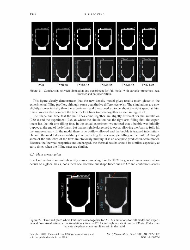
1388 R. R. RAO ET AL.
Figure 21. Comparison between simulation and experiment for full model with variable properties, heattransfer and polymerization.
This figure clearly demonstrates that the new density model gives results much closer to theexperimental filling profiles, although some quantitative differences exist. The simulations are nowslightly slower initially than the experiment, and then speed up to be about the right speed at latertimes. We can also compare the time for knit lines to come together as seen in Figure 22.
The shape and time that the knit lines come together are slightly different for the simulation(220 s) and the experiment (236 s), where the simulation has the right arm filling first, the exper-iment has the left arm filling first. In the actual experiment we noticed that a bubble was initiallytrapped at the end of the left arm, but that a slight leak seemed to occur, allowing the foam to fully fillthe arm eventually. In the model there is no outflow allowed and the bubble is trapped indefinitely.Overall, the model does a credible job of predicting the macroscopic filling of the mold. Althoughsome of the subtleties of the flow are obviously missing, it is an adequate production-scale model.Because the thermal properties are unchanged, the thermal results should be similar, especially atearly times when the filling rates are similar.
4.3. Mass conservation
Level set methods are not inherently mass conserving. For the FEM in general, mass conservationoccurs on a global basis, not a local one, because our shape functions are C o and continuous across
Figure 22. Time and place where knit lines come together for ARIA simulations for full model and experi-mental flow visualization: left is simulation at timeD 220.1 s and right is data at timeD 236.4 s. Red arrows
indicate the place where knit lines join in the mold.
Published 2011. This article is a US Government work andis in the public domain in the USA.
Int. J. Numer. Meth. Fluids 2011; 68:1362–1392DOI: 10.1002/fld

A LEVEL SET METHOD TO STUDY FOAM PROCESSING: A VALIDATION STUDY 1389
element boundaries. This can lead to areas with mass sources and sinks, which then can lead to eitheran increase or a decrease in the mass of phases A and B. Foam self-expansion can be particularlysusceptible to mass loss issues compared with incompressible flow problems because volume andvelocity generation occur via the continuity equation, which also includes the stabilization terms.Sources of mass loss include pressure jumps at the interface because of capillarity, time integration,pressure stabilization, level set advection, level set renormalization and the diffuse interface inter-acting with small geometric features or large curvatures. Using a constant time step and keeping theCourant number under 0.25 seems to improve the performance of the first-order Backward–Eulertime integration [48].
Mass conservation can be estimated in the high-end visualization tool Ensight [47] by integratingthe density over the foam phase to get the mass as a function of time and comparing this to theinitial mass
mass.t/D
ZV
.�foam/dV . (53)
The algorithm above was designed to keep mass loss to a minimum, but some mass loss did occur.For the time-dependent density function, using renormalization based on checking the gradient ofthe level set function that was carried out at a maximum of every three times step, mass is conservedto 2% if we look at the deviation. The mass as a function of time is shown in Figure 23 for both thecoarse and fine mesh. The initial mass is plotted for comparison and is used for our exact solution.This is a stringent test because both the density and volume of integration are changing with time.
The numerical mass goes above and below the analytical solution, which is disconcerting.However, the noise in the mass is relatively small and improves somewhat with mesh refinement.
We can also look at some other measures of the error in the solution such as the L2 norm of errorin mass as defined
kek2 D
0BB@numPiD1
.mass.ti /�massinit/2
numPiD1
.massinit/2
1CCA1=2
, (54)
where num is the number of points in the mass as a function of time plot. We can also look at theintegral of the error with time
I2 D
tDtfillZtD0
.mass.ti /�massinit/2dt . (55)
Figure 23. Mass conservation as a function of time for coarse and fine mesh solutions.
Published 2011. This article is a US Government work andis in the public domain in the USA.
Int. J. Numer. Meth. Fluids 2011; 68:1362–1392DOI: 10.1002/fld

1390 R. R. RAO ET AL.
Table VI. Error norms for coarse and refined meshes.
Mesh Number of nodes kek2 I2
Coarse 114,600 0.01114 2.68Refined 916,512 0.01055 2.55
The error norms are summarized in Table VI for the coarse and fine meshes.Here, we can see that we do get a reduction in the error with mesh refinement, but this reduc-
tion is quite small considering how much finer the mesh is and how drastic the increase inrequired computational time. This is another indication that our coarse mesh was adequate for foamexpansion studies.
5. CONCLUSIONS AND FUTURE WORK
We have developed a production scale model that can be used to study foam self-expansion incomplex geometries. The model is based on a finite element/level set implementation in the ARIAmodule of the SIERRA mechanics framework. The foam model is based on a continuum theory thathomogenizes the effects of gas bubbles into a time-dependent density model. ARIA was run on upto 68 processors to obtain results in a test fixture that included nonisothermal effects, in additionto curing, variable properties, and dilatational viscosity. The results from the model were comparedwith flow visualization data. The model performed fairly well, although there were some quanti-tative differences between the filling rates and shapes thought to come from uncertainties in thedensity model.
This model is an engineering design tool that will allow us to study processing variables suchas temperature and Fluorinert and air concentrations, and the effect of gate and vent locations foroptimizing the foam encapsulation process. It has many good features, such as: (i) it is reasonablyrobust numerically; (ii) it is fast enough that it can be run in complex geometries of real applications;(iii) it is fairly easy to understand and populate via simple experiments and experimental analysisand can be applied to other foams; and (iv) it can predict trends for engineering optimization.
However, there is obviously room for improvement and we would like to develop a more quan-titative model. We are currently developing a detailed treatment of the Fluorinert nucleation andgrowth that does not rely wholly on the density model for the correct foaming. The effect of evolv-ing shear viscosity never slows the predicted expansion of the fluid because the density model doesnot include the effect of cure. The normal stress from the dilatational viscosity also does not affectthe dynamics of mold filling because a Newtonian model without this effect shows the same behav-ior [49]. A more physics-based model for bubble expansion, which includes the effect of evolvingviscosity and elasticity of the polymer and capillarity all coupled to Fluorinert nucleation and boil-ing, would produce a more realistic model. Missing from our current model is this effect, along withthe density gradients created by the buoyancy of the gas bubbles relative to the epoxy that result increaming. We will include the effects of bubble transport using a model similar to models for glassmicroballoons in curing epoxy, which proved useful for predicting the complex flow of floatingmicroballoons in curing epoxy in complex geometries [50].
ACKNOWLEDGEMENTS
We appreciate the funding provided by Accelerated Strategic Computing (ASC) to develop this model,implement it in SIERRA/ARIA, and document the results. The model would be nothing without the experi-mental team who made experimental discoveries for model development, determined parameters to populatethe model, and provided validation data. The experimental team, in addition to authors Lisa Mondy and DougAdolf, included Anne Grillet, Ed Russick, Chris Brotherton, Chris Bourdon, Allen Gorby, Ray Cote, JaimeCastañeda, and Kyle Thompson. Andy Kraynik has been invaluable for pointing us in the right direction forcorrelations from the foam literature and his general knowledge of foam. Jim Mahoney from Kansas CityPlant has inspired this project by politely asking for a foam self-expansion modeling tool because none arecommercially available at the present time. He has also tirelessly provided meshes and geometries, addingand changing the boundary conditions at our insistence.
Published 2011. This article is a US Government work andis in the public domain in the USA.
Int. J. Numer. Meth. Fluids 2011; 68:1362–1392DOI: 10.1002/fld
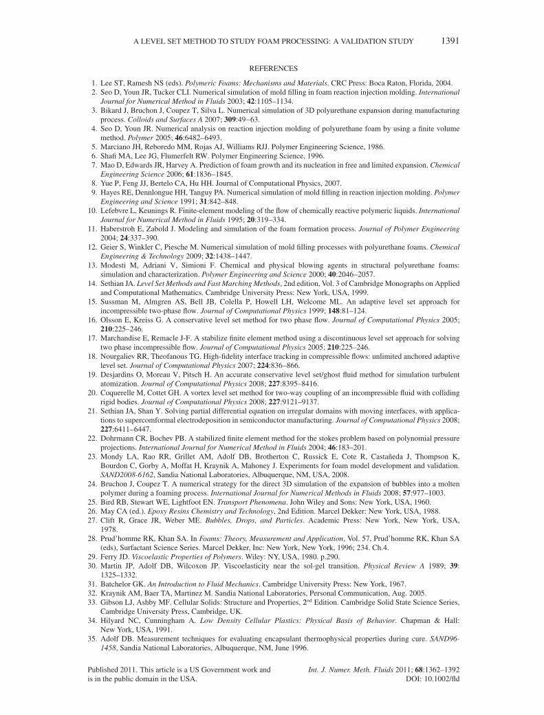
A LEVEL SET METHOD TO STUDY FOAM PROCESSING: A VALIDATION STUDY 1391
REFERENCES
1. Lee ST, Ramesh NS (eds). Polymeric Foams: Mechanisms and Materials. CRC Press: Boca Raton, Florida, 2004.2. Seo D, Youn JR, Tucker CLI. Numerical simulation of mold filling in foam reaction injection molding. International
Journal for Numerical Method in Fluids 2003; 42:1105–1134.3. Bikard J, Bruchon J, Coupez T, Silva L. Numerical simulation of 3D polyurethane expansion during manufacturing
process. Colloids and Surfaces A 2007; 309:49–63.4. Seo D, Youn JR. Numerical analysis on reaction injection molding of polyurethane foam by using a finite volume
method. Polymer 2005; 46:6482–6493.5. Marciano JH, Reboredo MM, Rojas AJ, Williams RJJ. Polymer Engineering Science, 1986.6. Shafi MA, Lee JG, Flumerfelt RW. Polymer Engineering Science, 1996.7. Mao D, Edwards JR, Harvey A. Prediction of foam growth and its nucleation in free and limited expansion. Chemical
Engineering Science 2006; 61:1836–1845.8. Yue P, Feng JJ, Bertelo CA, Hu HH. Journal of Computational Physics, 2007.9. Hayes RE, Dennlongue HH, Tanguy PA. Numerical simulation of mold filling in reaction injection molding. Polymer
Engineering and Science 1991; 31:842–848.10. Lefebvre L, Keunings R. Finite-element modeling of the flow of chemically reactive polymeric liquids. International
Journal for Numerical Method in Fluids 1995; 20:319–334.11. Haberstroh E, Zabold J. Modeling and simulation of the foam formation process. Journal of Polymer Engineering
2004; 24:337–390.12. Geier S, Winkler C, Piesche M. Numerical simulation of mold filling processes with polyurethane foams. Chemical
Engineering & Technology 2009; 32:1438–1447.13. Modesti M, Adriani V, Simioni F. Chemical and physical blowing agents in structural polyurethane foams:
simulation and characterization. Polymer Engineering and Science 2000; 40:2046–2057.14. Sethian JA. Level Set Methods and Fast Marching Methods, 2nd edition, Vol. 3 of Cambridge Monographs on Applied
and Computational Mathematics. Cambridge University Press: New York, USA, 1999.15. Sussman M, Almgren AS, Bell JB, Colella P, Howell LH, Welcome ML. An adaptive level set approach for
incompressible two-phase flow. Journal of Computational Physics 1999; 148:81–124.16. Olsson E, Kreiss G. A conservative level set method for two phase flow. Journal of Computational Physics 2005;
210:225–246.17. Marchandise E, Remacle J-F. A stabilize finite element method using a discontinuous level set approach for solving
two phase incompressible flow. Journal of Computational Physics 2005; 210:225–246.18. Nourgaliev RR, Theofanous TG. High-fidelity interface tracking in compressible flows: unlimited anchored adaptive
level set. Journal of Computational Physics 2007; 224:836–866.19. Desjardins O, Moreau V, Pitsch H. An accurate conservative level set/ghost fluid method for simulation turbulent
atomization. Journal of Computational Physics 2008; 227:8395–8416.20. Coquerelle M, Cottet GH. A vortex level set method for two-way coupling of an incompressible fluid with colliding
rigid bodies. Journal of Computational Physics 2008; 227:9121–9137.21. Sethian JA, Shan Y. Solving partial differential equation on irregular domains with moving interfaces, with applica-
tions to supercomformal electrodeposition in semiconductor manufacturing. Journal of Computational Physics 2008;227:6411–6447.
22. Dohrmann CR, Bochev PB. A stabilized finite element method for the stokes problem based on polynomial pressureprojections. International Journal for Numerical Method in Fluids 2004; 46:183–201.
23. Mondy LA, Rao RR, Grillet AM, Adolf DB, Brotherton C, Russick E, Cote R, Castañeda J, Thompson K,Bourdon C, Gorby A, Moffat H, Kraynik A, Mahoney J. Experiments for foam model development and validation.SAND2008-6162, Sandia National Laboratories, Albuquerque, NM, USA, 2008.
24. Bruchon J, Coupez T. A numerical strategy for the direct 3D simulation of the expansion of bubbles into a moltenpolymer during a foaming process. International Journal for Numerical Methods in Fluids 2008; 57:977–1003.
25. Bird RB, Stewart WE, Lightfoot EN. Transport Phenomena. John Wiley and Sons: New York, USA, 1960.26. May CA (ed.). Epoxy Resins Chemistry and Technology, 2nd Edition. Marcel Dekker: New York, USA, 1988.27. Clift R, Grace JR, Weber ME. Bubbles, Drops, and Particles. Academic Press: New York, New York, USA,
1978.28. Prud’homme RK, Khan SA. In Foams: Theory, Measurement and Application, Vol. 57, Prud’homme RK, Khan SA
(eds), Surfactant Science Series. Marcel Dekker, Inc: New York, New York, 1996; 234. Ch.4.29. Ferry JD. Viscoelastic Properties of Polymers. Wiley: NY, USA, 1980. p.290.30. Martin JP, Adolf DB, Wilcoxon JP. Viscoelasticity near the sol-gel transition. Physical Review A 1989; 39:
1325–1332.31. Batchelor GK. An Introduction to Fluid Mechanics. Cambridge University Press: New York, 1967.32. Kraynik AM, Baer TA, Martinez M. Sandia National Laboratories, Personal Communication, Aug. 2005.33. Gibson LJ, Ashby MF. Cellular Solids: Structure and Properties, 2nd Edition. Cambridge Solid State Science Series,
Cambridge University Press, Cambridge, UK.34. Hilyard NC, Cunningham A. Low Density Cellular Plastics: Physical Basis of Behavior. Chapman & Hall:
New York, USA, 1991.35. Adolf DB. Measurement techniques for evaluating encapsulant thermophysical properties during cure. SAND96-
1458, Sandia National Laboratories, Albuquerque, NM, June 1996.
Published 2011. This article is a US Government work andis in the public domain in the USA.
Int. J. Numer. Meth. Fluids 2011; 68:1362–1392DOI: 10.1002/fld

1392 R. R. RAO ET AL.
36. Edwards HC. SIERRA framework version 3: core theory and design. SAND2002-3616, Sandia National Laboratories,Albuquerque, NM, November 2002.
37. Notz PK, Subia SR, Hopkins MM, Moffat HK, Noble DR. ARIA manual aria 1.5: user’s manual. SAND2007-2734,Sandia National Laboratories, Albuquerque, NM, April, 2007.
38. Rao RR, Mondy LA, Noble DR, Hopkins MM, Notz PK, Baer TA, Halbleib LL, Yang P, Burns GR, GrilletAM, Brooks CF, Cote RO, Castaneda JN. Modeling injection molding of net-shape active ceramic components.SAND2006-6786, Sandia National Laboratories, Albuquerque, NM, November 2006.
39. Mondy LA, Rao RR, Brooks CF, Noble DR, Givler RC, Sun AC, Kraynik AM, Baer TA, Wilkes ED, Notz PK,Hopkins MM, Grillet AM, Cote RO, Castaneda JN, Adolf DB, Mahoney J, Berchtold K, Brooks M, Graham A. Wet-ting and free surface flow modeling for potting and encapsulation. SAND2007-3316, Sandia National Laboratories,Albuquerque, NM, May 2007.
40. Brackbill JU, Kothe DB, Zemach C. A continuum method for modeling surface-tension. Journal of ComputationalPhysics 1992; 100:335–354.
41. Jacqmin D. Three dimensional computations of droplet collisions, coalescence, and droplet/wall interactions using acontinuum surface-tension method. AIAA-95-0883, 1995.
42. Sussman M, Fatemi E. An efficient, interface-preserving level set redistancing algorithm and its application tointerfacial incompressible fluid flow. SIAM Journal of Scientific Computing 1999; 20:1165–1191.
43. Hughes TJR. The Finite Element Method. Dover Publications: New York, USA, 2000.44. Donea J. A Taylor-Galerkin method for convective transport problems. International Journal for Numerical Method
in Engineering 1984; 20:101–119.45. Trilinos. http://trilinos.sandia.gov, 2010.46. Kern DQ. Process Heat Transfer. McGraw-Hill Book Company: New York, USA, 1950.47. Ensight. Computational Engineering International, www.ensight.com, 2011.48. Finlayson BA. Numerical Methods for Problems with Moving Fronts. Ravenna Park Publishing: Seattle, USA, 1992.49. Rao RR, Mondy LA, Moffat HK, Noble DR, Notz PK, Adolf DB, Baer TA. Foam process models. SAND2008-6094,
Sandia National Laboratories, Albuquerque, NM, USA, 2008.50. Rao RR, Mondy LA, Altobelli SA. Instabilities during batch sedimentation in geometries containing obstacles:
a numerical and experimental study. International Journal for Numerical Method in Fluids 2007; 55:723–735.51. CUBIT Geometry and Mesh Generation Toolkit, http://cubit.sandia.gov, 2011.52. Mondy LA, Rao RR, Lindgren ER, Sun AC, Adolf DB, Retallack C, Thompson K. Modeling coupled migration and
settling of particulates in curing filled epoxies. Journal of Applied Polymer Science 2011; 122:1587–1598.
Published 2011. This article is a US Government work andis in the public domain in the USA.
Int. J. Numer. Meth. Fluids 2011; 68:1362–1392DOI: 10.1002/fld