A Large-Scale Study of Microbial and Physico-Chemical Quality of Selected Groundwaters

and Surface Waters in the North West Province, South Africa

Report to the

Water Research Commission

by

CC Bezuidenhout and the North-West University Team

WRC Report No. 1966/1/13

ISBN 978-1-4312-0400-7

APRIL 2013

ii

Obtainable from Water Research Commission Private Bag X03 GEZINA, 0031 orders@wrc.org.za or download from www.wrc.org.za This report contains a CD with raw data measurements.

DISCLAIMER

This report has been reviewed by the Water Research Commission (WRC) and approved for publication. Approval does not signify that the contents necessarily reflect the views and policies of the WRC, nor does mention of trade names or commercial products constitute

endorsement or recommendation for use.

© WATER RESEARCH COMMISSION

iii

North-West University Project team and their contributions

Carlos Bezuidenhout Project Leader, Compiled this report and supervised Simone Ferreira, Lesego Molale, Deidre van Wyk (Co- supervised), Karen Jordaan, Werner Ressouw, Wesley van Oeffelen, Suranie Prinsloo (Co-supervised), Rasheed Adeleke Owen Rhode Supervise yeast work (ARC – Potchefstroom) Thami Sitebe Supervise the phage work Collins Ateba Supervise the phage work Rialet Pieterse Supervise the cytoxicity Rasheed Adeleke Enterovirus analysis Maureen Taylor Phage and enterovirus analysis (University of Pretoria) Simone Ferreira Groundwater physico-chemical and bacteriological analysis Lesego Molale Surface water physico-chemical and bacteriological analysis Deidre van Wyk Surface water physico-chemical and yeast analysis Keabetswe Mabote Phage analysis Werner Ressouw Phage analysis – Mooi River Karen Jordaan Denaturing gradient gel electrophoresis and high throughput sequencing analysis Wesley van Oeffelen (Avans multiplex PCR analysis of E. coli Hogen School, Netherlands) Suranie Prinsloo Cytoxicity assay development and analysis Jaco Bezuidenhout Assisted with the statistics

iv

v

EXECUTIVE SUMMARY

BACKGROUND AND RATIONALE

Water from the North West Province (NWP) catchment areas supports prosperous gold and

platinum mining, manufacturing industries, agricultural sector as well as a growing urban and

rural population. This land-locked province thus contributes generously to the Gross

Domestic Product of South Africa. However, water allocation for the province has almost

reached the quota available, based on surface water estimates. Furthermore, there are

reports that the source water within the catchment may be exposed to pollution from various

sources but particularly from economic activities. These reports have demonstrated that

several surface waters and groundwaters are faecally contaminated and some with

opportunistic pathogenic bacteria.

Faecal pollution of surface waters has been blamed on service delivery problems in several

peri-urban areas and small towns. There are also reports of poorly treated and in some

cases untreated effluent being discharged into rivers and other receiving waters. This

practice has health, economic as well as environmental implications. The growth in the

agricultural and mining sectors has resulted in increased water requirements as well as

pollution. These developments have also played a role in human population distribution

dynamics. Such economic activities were responsible for the development of major growth

points in the province.

Mining activities are mainly centred in the eastern part of the province and the agricultural

development across the province. Mining operations were (in some cases still are)

responsible for decant of heavy metal-containing water of low pH (acid mine drainage: AMD)

into surface water. This has devastating ecological and economics effects. The real impacts

of the AMD on groundwater in the North West Province are undetermined. Water pollution

from agricultural runoff from livestock farming, including poultry farming and feedlots as well

as several other practices in the province is also undetermined.

Rainfall in the eastern and central parts of the province is higher than the western part. The

latter borders on and is part of the Kalahari Desert. Further social and economic

developments as well as climate change will impact on the anticipated water availability,

requirements and quality of water. Baseline data in these categories will be important for

long-term planning. Water requirements are national priorities and processes such as

National Water Resource Strategy are in place. However, detailed large water quality studies

vi

have not been conducted. The present study was an effort to address this gap. It extended

the WRC-funded work done by Bezuidenhout (2011).

AIM

1. To determine the water quality of surface and groundwater in the North West

Province from chemico-physical and microbiological perspectives.

2. To determine the profile of selected gastroenteritis-associated pathogens in the

contaminated water sources.

3. To investigate the usefulness of molecular fingerprinting data in microbial water

quality determination.

4. To determine the cytotoxic effects of associated with consumption of untreated water

as well as such effects exerted by some of the indicator mycological and bacterial

species isolated from the water sources.

5. To investigate potential risk of consuming such water without any prior treatment.

6. To provide an overview of previous large-scale water quality studies conducted

nationally and internationally.

7. To generate a report on whether human health risks could be associated with current

trends of water provision in the North West Province and if necessary suggest

improvement strategies.

The following describes the scope of the work in each chapter:

Chapter 2: The purpose of this work was to generate data on microbiological and physico-

chemical quality of surface water sources in the North West Province. A secondary goal was

to establish skills with respect to several research methodologies. These technologies

include determining levels of (a) culturable indicator bacteria (faecal coliforms, enterococci),

(b) yeasts, (c) pathogenic E. coli (d) bacteria by culture independent microbial detection

methods (Denaturing Gradient Gel Electrophoresis and High Throughput Sequencing) and

(e) enteroviruses and bacteriophages.

vii

Chapter 3: The purpose was to generate data on microbiological and physico-chemical

quality of groundwater using some of the methodologies and methods referred to in

Chapter 2.

Chapter 4: The purpose was to evaluate faecal sterol determination in water quality

applications in the North West Province.

Chapter 5: The purpose was to evaluate the various bacteria and fungi isolated during this

study for potential human health effects and to develop a cost an effective method to

determine the cytotoxicity effects of polluted water on intestinal cells.

Chapter 6: The purpose was to conduct a social and water management study in order to

identify the most important social aspects for future research and interventions in the

province.

METHODOLOGY

Water samples were collected at specific time periods from selected groundwater and

surface water sources in the North West Province using standard procedures. An effort was

made to include dry winter as well as wet summer sampling periods for each of the sites.

The groundwater sampling sites were grouped into sampling areas so groundwater locations

in this report refer to an area, not specific boreholes.

Standard methodologies were used to collect and analyse the water samples. Global

positioning data (GPS waypoints) were recorded and used to generate the sampling maps.

Certain physical and chemical (temperature, pH, electrical conductivity) parameters were

measured on site using multi-probe equipment. Chemical parameters such as chemical

oxygen demand, nitrates, phosphates etc. were measured in the laboratory using Hach kits

and equipment. The levels of faecal indicators and other microbial organisms were

determined using standard or previously-published methods. Standard biochemical and DNA

sequencing methods were used for identification of microbes. The presence of E. coli and

pathogenic E. coli were determined in water using direct DNA isolation and PCR. Faecal

sterol levels were determined by the Szűcs method which involves liquid-liquid extraction

and resolution by Gas Chromatography-Mass Spectrometry. Levels of bacteriophages were

determined by standard methods and enterovirus by qPCR based methodology.

A sequential exploratory mixed-methods design was used for the social water management

study. A mixed-methods approach includes the use of both qualitative and quantitative

viii

research methods to collect, analyse and interpret the research data. Interviews, focus group

discussions and observations (n = 25 participants) were used as the main data gathering

methods during the qualitative phase. This was followed by the development of a research

questionnaire and a community survey (n = 1 000 participants) during the quantitative phase

of the study.

RESULTS AND DISCUSSION

Microbiological and physico-chemical quality of surface water sources

Selected river systems covering the upper middle and lower Vaal river management areas

were targeted. Average physico-chemical and microbial levels measured at some sites

during the 2010 and 2011 seasons were elevated. Some exceeded the Target Water Quality

Range (TWQR) for full and intermediate recreational contact, livestock watering and

irrigation. Elevated electrical conductivity when compared to TWQR for drinking water was

not at levels likely to cause health impacts. However, this elevated EC could be indicative of

increasing salinisation occurring. This may have long-term effects on agriculture activities

but also on drinking water production. Electrical conductivity should be flagged as a

parameter that is critical to monitor.

Enterococcus spp. as well as Escherichia coli were isolated from various surface water

sources. Isolation of enterococci such as E. faecium and E. faecalis from surface waters

illustrates that any full contact activity in the water is risky and could result in infectious

disease. Bacteriophage data supported the general findings of the bacterial analysis, namely

that many of the water sources in the North West Province have some form of faecal

pollution. The following yeast genera were also isolated and identified in surface waters:

Candida, Clavispora, Cryptococcus, Cystofilobasidium Hanseniaspora, Meyerozyma, Pichia,

Rhodotorula, Saccharomyces, Sporidiobolis, and Wickerhamomyces. Amongst these are

several opportunistic pathogenic species that could cause invasive infections when

individuals come into contact with contaminated water.

Baseline culture-independent molecular profiling (Polymerase Chain Reaction Denaturing

Gradient Gel Electrophoresis (PCR-DGGE) and Next Generation Sequencing (NGS)) data of

the dominant bacterial communities in the Vaal River are also provided. Although DGGE

profiling has some limitations it allowed for the identification of the bacterial community

composition and dynamics in the planktonic component in this river system. Next generation

sequencing or high through-put sequencing (HTS) analysis presented a better resolution of

the bacterial diversity and dynamics in the Vaal River. This technology was not suitable for

ix

detecting faecal indicator bacteria in surface water samples that contained known high levels

of E. coli and enterococci.

Results presented here demonstrated that some of the wastewater treatment plants

(WWTPs) were decanting huge concentrations of enterovirus particles into surface water

sources. This was probably due to the operational challenges at the plants. Some other

plants in the province were operating in such a manner that up to 99.99% of enteroviruses

were removed. Impacts of municipal WWTPs as well as other forms of faecal pollution on

virus diversity and dynamics in water sources should be further investigated. Such a study

should focus on the percentage of viable viruses that are reaching the water bodies and the

epidemiology thereof. In such a virology study the presence of other relevant viruses should

also be targeted. Furthermore, detection of bacteriophages in the surface waters that are

associated with faecal pollution supports the finding that some of the targeted surface water

sources in the North West Province are faecally polluted.

Microbiological and physico-chemical quality of groundwater

In the North West Province more than 80% of the rural community depend on groundwater

for all their water needs. The approach was to mainly target boreholes that provided water

for domestic use. This included urban, peri-urban and rural areas. A total of 114 boreholes

were sampled. Physico-chemical analyses demonstrated that the pH and EC levels were at

acceptable ranges for domestic use. However, it was found that only 28% of the boreholes

tested complied with the South African TWQR for nitrate (<6 mg/ℓ), and 43% of the

boreholes had nitrate levels greater than 20 mg/ℓ. This study also demonstrated that

groundwater from the North West Province is vulnerable to nitrate contamination.

In 2009 49% of the 76 boreholes tested were positive for faecal coliforms and 67% for faecal

streptococci. Forty seven percent of these boreholes were also positive for presumptive

P. aeruginosa and 7% for S. aureus. 33% of the boreholes had heterotrophic plate bacteria

exceeding 1000 cfu/ml. In 2010, 38 boreholes were sampled. Of these 55% were positive for

faecal coliforms and 63% for faecal streptococci. During this sampling period 55% of the

boreholes were positive for P. aeruginosa. Detection of faecal indicators was higher in the

warm wet seasons than the cold dry season. This was observed in both the number of

positive results as well as levels detected. Members of the Enterobacteriaceae family

identified included E. coli and K. pneumonia.

Based on MLGA results, 34% of the boreholes sampled in 2010 were positive for E. coli.

However, using multiplex PCR on DNA directly isolated from water samples it was found that

x

E. coli was present in 47% of boreholes. This indicates that the membrane filtration

approach underestimated the presence of E. coli in borehole water in the NWP. Using

FC/FS (faecal coliform/faecal streptococci) ratio determination, it was estimated that at least

14% of the boreholes tested had FC/FS ratio >2, indicating potential human faecal

contamination.

Next generation sequencing (or high through-put sequencing) results provided data on the

microbial diversity in borehole water of the NWP. This method is rapid and provided

information about the bacterial community structure in these water samples. It was

demonstrated that the winter and summer bacterial compositions were different. In the

summer samples there were Gamma and Beta proteobacteria as well as Actinobacteria

present. Enterobacter sp., Proteus sp., Stenotrophomonas maltophilia are species that were

always detected among the Gamma proteobacteria. Sequences from E. coli as well as

Pseudomonas sp. and S. aureus were also detected in the summer samples. These results

are consistent with the results from the culture dependent method. Next generation

sequencing (or HTS) thus holds promise as a method for monitoring bacterial indicator

species in groundwater. This, however, needs to be further tested.

The results presented here indicated that microbiological quality of groundwater in the North

West Province may be of concern as more than 75% of boreholes were positive for faecal

pollution. This indicates that groundwater should be tested and treated before being

supplied to communities. It was, however, demonstrated that 23% of the boreholes tested

negative for both faecal coliforms and faecal streptococci. This result indicates that there are

boreholes where no faecal pollution has occurred. This could be due to protection of the

borehole and thus the aquifer. Management practices should be put in place to prevent

pollution of aquifers.

Faecal sterol determination in water quality applications

In this study the Szűcs method, an established method for detecting faecal sterols in water,

was used to detect six target sterols (coprostanol, cholesterol, dehydrocholesterol,

stigmasterol, β-sitosterol, and stigmastanol) in water samples from the NWP. Wastewater

treatment plant influent and effluent samples were collected and analysed for human faecal

sterol biomarkers. Environmental water samples were spiked with faeces from cattle,

chickens, horses, pigs, and sheep. All the samples were subjected to liquid-liquid extraction,

silylation and derivatisation. Derivatised samples were analysed by GC-MS. The method

was evaluated for quantitation and differences between the water samples from each

species. Standard curve assays were linear up to 160 ng/ℓ and the limit for quantification

xi

was 20 ng/ℓ. Coprostanol was the human faecal sterol biomarker, while herbivore profiles

were dominated by terrestrial sterol biomarkers (stigmasterol and stigmastanol). Differences

in sterol fingerprints and concentrations between various animals and humans provide the

opportunity to determine the origin of faecal pollution.

Water samples collected from boreholes and rivers were analysed for faecal sterols,

physico-chemical properties and bacteriological quality. Coprostanol and cholesterol were

detected in one groundwater sample. These results were in some cases supported by

bacteriological data and in other cases not. Sterols may become bound to soil particles. It is

therefore not expected that sterols will be detected in groundwater. Their detection in

groundwater in this study should therefore be further explored.

Surface water samples were also analysed for faecal sterols using the Szűcs method.

Cholesterol was detected in some samples and was the only faecal sterol detected. This

indicates that the faecal pollution at these sites were likely to be from animals, not humans.

Faecal sterol analysis is a powerful method and has potential to distinguish between faecal

pollution from various animal as well as human sources.

Potential human health effects

The main human health concern is the high level of nitrates in some of the groundwater

sources, some exceeding the 20 mg/ℓ level that could cause methaemaglobinemia. This was

not the case with surface water sources in associated areas. Signs of salinisation were

observed for some of the surface water samples. However, at the moment this cannot be

linked to human health concerns.

Faecal indicator and opportunistic bacteria were regularly detected in surface and

groundwater sources of the NWP. It was shown that pathogenic E. coli may also be present

among the environmental E. coli population. Various known opportunistic pathogenic

enterococci were regularly detected in surface waters. Pseudomonas spp. were also

regularly detected in groundwaters. Among the yeasts isolated several opportunistic

pathogenic species were also regularly detected. These studies were conducted over two

separate sampling periods, about one year apart. The results suggest that these bacteria

(and in the case of surface waters also yeast) could be ubiquitous. This is cause for concern

and regular monitoring of such sites is proposed. It could indicate that pathogenic

microorganisms such as viruses (enterovirus, adenovirus and hepatitis A & B) and bacteria

(Vibrio cholerae, Shigella spp. Yersina spp. and Enterocolitica spp.) may also be present in

these water sources. This study has also detected bacteriophages associated with faecal

xii

pollution. The phages are surrogates for human viruses. What the study has further

demonstrated is that entoviruses are being discharged into receiving surface waters. This

study did not determine whether the viruses were viable. However, if one considers that

faecal bacteria detected in the water sources were all viable there is a chance that the

viruses may also be viable. The detection of virus genetic material in a water source is thus

a cause for concern. All these findings demonstrate that people in the North West Province

that directly use untreated water for household purposes or recreation may be exposed to

several pathogenic or opportunistic pathogens. Such exposures imply that the health of

these individuals may be compromised.

Amongst the enterococci isolates from surface waters, up to 20% displayed β-haemolysis, a

character that demonstrates the production of an enzyme that is associated with virulence.

Furthermore, dominant multiple antibiotic resistance patterns were observed for faecal

streptococci isolates at most sites in both years. Between 40 and 55% of the isolates were

resistant to selected β-lactam antibiotics including Penicillin G. Not all the isolates that were

resistant to Penicillin G were resistant to Ampicillin or Amoxillin. A large proportion was also

resistant to Vancomycin. Up to 68% was resistant to Neomycin and 56% to Ciprofloxacin.

Most of the isolates (up to 99%) were susceptible to Streptomycin. All β-haemolysis positive

isolates (potential pathogenic) were resistant to 3 and more antibiotics from various antibiotic

groups. Similar results were observed for both study periods

Several of the faecal coliform isolates from surface water were resistant to multiple

antibiotics, especially β-lactam antibiotics. Table 1 is a summary of the percentage of faecal

coliforms that were resistant to antibiotics.

Table 1: Antibiotic resistance profiles (%) among faecal coliforms isolated in 2009 and 2010.

2009 2010

Amoxyllin 54 21

Ampicillin 41 15

Cephalothin 40 42

Oxytetracyclin 30 22

Trimetroprim 11 8

Fewer isolates in 2010 were resistant to β-lactam antibiotics compared to those from 2009.

However, resistance to Cephalothin, a cephem β-lactam, was similar for both sampling

periods.

xiii

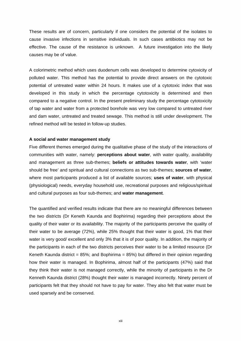
These results are of concern, particularly if one considers the potential of the isolates to

cause invasive infections in sensitive individuals. In such cases antibiotics may not be

effective. The cause of the resistance is unknown. A future investigation into the likely

causes may be of value.

A colorimetric method which uses duodenum cells was developed to determine cytoxicity of

polluted water. This method has the potential to provide direct answers on the cytotoxic

potential of untreated water within 24 hours. It makes use of a cytotoxic index that was

developed in this study in which the percentage cytotoxicity is determined and then

compared to a negative control. In the present preliminary study the percentage cytotoxicity

of tap water and water from a protected borehole was very low compared to untreated river

and dam water, untreated and treated sewage. This method is still under development. The

refined method will be tested in follow-up studies.

A social and water management study

Five different themes emerged during the qualitative phase of the study of the interactions of

communities with water, namely: perceptions about water, with water quality, availability

and management as three sub-themes; beliefs or attitudes towards water, with ‘water

should be free’ and spiritual and cultural connections as two sub-themes; sources of water,

where most participants produced a list of available sources; uses of water, with physical

(physiological) needs, everyday household use, recreational purposes and religious/spiritual

and cultural purposes as four sub-themes; and water management.

The quantified and verified results indicate that there are no meaningful differences between

the two districts (Dr Keneth Kaunda and Bophirima) regarding their perceptions about the

quality of their water or its availability. The majority of the participants perceive the quality of

their water to be average (72%), while 25% thought that their water is good, 1% that their

water is very good/ excellent and only 3% that it is of poor quality. In addition, the majority of

the participants in each of the two districts perceives their water to be a limited resource (Dr

Keneth Kaunda district = 85%; and Bophirima = 85%) but differed in their opinion regarding

how their water is managed. In Bophirima, almost half of the participants (47%) said that

they think their water is not managed correctly, while the minority of participants in the Dr

Kenneth Kaunda district (28%) thought their water is managed incorrectly. Ninety percent of

participants felt that they should not have to pay for water. They also felt that water must be

used sparsely and be conserved.

xiv

With regard to their beliefs and attitudes towards water, almost half of the participants said

that they have a spiritual connection with water (45%) and that they use water for example to

cleanse themselves or others after a funeral ceremony (75%) or to make contact with their

ancestors (45%).

The study also confirmed that the majority of households make use of municipal water

(77%). Sources of water did not differ greatly between the two districts, except in regard to

the harvesting of rain water. In the Bophirima district, communities make more use of rain

water harvesting (32%), compared to the Dr Kenneth Kaunda district where only 11%

harvest water. Other sources of water such as a borehole with a windmill (21%), or a

borehole with an electrical pump (10%), seasonal pans (6%), fountains (5%), dams and

rivers (4%) and wells (4%) are used to a lesser extent.

A number of uses differed statistically and practically between the two districts. In the

Bophirima district, traditional uses such as using water to drive out evil spirits (cleansing

themselves or members of their family or house) differed from the Dr Keneth Kaunda district

(Table 2). It demonstrates that more individuals in the Bophirima district uses their water for

the purposes listed compared to the Dr Kenneth Kaunda district participants.

Table 2: Recreational and traditional uses of water (%).

Bophirima Dr Kenneth Kaunda

Drive out spirits 75 50

Make traditional medicine 81 57

Recreational purposes 75 55

Harvest food 43 20

Livestock watering 70 28

Other popular uses of water that scored above 88% include the use of water for house

building or other physical structures (for example in combination with soil) (94.2%), to cook

their food (99%), to drink (98%), and to flush their toilet (96%). More than 90% indicated that

water helps them when they are fasting (92%). Ninety seven percent indicated that water is

used during religious ceremonies (e.g. washing their own or other’s feet before church)

Almost all the participants indicated that they use water to wash their goods (cleaning of

physical objects other than themselves) (99.3%). More than 19% indicated that they use

water for gardening (domestic plants) (93.2). Eighty eight percent indicated that they use

water to make traditional beer (umqhombothi).

xv

The use of water for self-cleansing (enema) seemed less popular (68%). Seventy six percent

indicated that they use water to initiate the traditional healer/s in their community. More than

60% indicated that they use water to wash themselves or others after a funeral service.

Amongst all the participants 28% were farmers using water on a large scale to produce

crops.

The majority of households still appear to make use of a tap in their yard. Fewer had access

to piped water in their houses. A section of the communities was still using a communal tap

for which they have to travel less than 50 meters or to a lesser extent more than 50 meters.

Finally, most households appear to store water inside their homes (65%) where it is cooled

down in most cases (83%). However, communities in the Bophirima district tend to store

water more often in containers outside their house (56%) compared to those participants

from the Dr Keneth Kaunda district (34%).

CONCLUSIONS

The purpose of the research was to conduct a large-scale study of microbial and physico-

chemical quality of selected surface waters and groundwaters in the North West Province,

South Africa. The sampling period was from 2009 to 2011. Results have shown various

trends.

• Nitrates in groundwater and salts in surface water are the main physico-chemical

hazards.

• A number of the groundwater and surface water sources in the North West Province

are polluted with faecal matter. The faecal pollution was demonstrated by various

methods including standard culture methods, direct DNA isolation and PCR, faecal

sterols, bacteriophages and in the case of groundwater, also next generation

sequencing.

• Bacteriophage and enterovirus data indicated that the sources may also contain

viruses that could be human pathogens.

• Large numbers of faecal coliforms and enterococci isolated in this study were

resistant to several antibiotic groups. This is cause for concern as it may eventually

have human and animal health as well as plant pathology implications.

• A cytoxicity test to determine the impacts of microorganisms on human cell cultures

was also developed as part of this study. It may be useful in future studies where

water quality and suitability for human consumption is determined. The adaptations

xvi

proposed in the study make it more rapid and precise but also, at the moment, more

costly to conduct.

• Baseline data on social aspects of source and drinking water management was also

provided for 6 communities from 2 of the 4 districts of the North West Province. The

study presented some data on how members from these communities interact with

and manage water. It also demonstrated that certain perceptions, beliefs and

behaviours are associated with these interactions. The results demonstrated that

water has important social and cultural meaning and importantly, that future

education programmes could build on knowledge existing with these communities.

RECOMMENDATIONS FOR FUTURE RESEARCH

• Sources of high EC values should be investigated as this could have serious

implications on soil quality in the province and by implication also food security. It

may eventually also impact on drinking water purification processes. Long-term

studies are thus necessary to generate data that would be useful for predictive

modelling studies. Such data would also be useful to provide advice to agricultural

and water purification authorities.

• Boreholes should be identified that may be vulnerable to certain types of

contamination. Data from the present study will be useful in identifying areas for

further investigation. Once identified appropriate interventions or treatment options

could then be put in place before such water is supplied as safe for human or animal

consumption.

• Sources of faecal pollution in surface water should also be identified and

programmes be put in place to ensure that this type of pollution is prevented. Data

from the present study could be used to identify specific areas in the selected rivers

that should be further investigated for faecal pollution sources.

• Results from this study have demonstrated that a full health risk assessment should

be conducted on some of the water sources in the province. This is needed

particularly within the context of the large section of the community of the NWP,

particularly in rural and peri-urban centres, that are immuno-compromised. At present

health effects of consuming the faecally-contaminated water could be under-reported

and a detailed study is thus necessary

• The cause of multiple antibiotic resistance and the mechanisms involved should be

further investigated. This was not established in the present study but should be

determined. Broader understanding of antibiotic resistance may provide means to

predict the spread of the resistance and in the process provide tools to curb the

xvii

spread. As more pathogens become resistant to available drugs the search for newer

more effective drugs may drain resources. This could result in a vicious circle in the

treatment of human, animal and plant infectious diseases.

• Future studies to determine the presence of E. coli and other indicators in the water

should be conducted also using PCR (qPCR) methods instead of only culture based

methods. Quantitative PCR (qPCR) is more accurate and rapid compared to plating

methods. Analysis times will be decreased and larger numbers of samples could be

analysed.

• In-depth HTS (and culture-based) analysis of the microbial diversity and water quality

in the surface and groundwater is recommended with the focal point on the

identification of specific species within the major key groups. This should be

conducted for viruses, bacteria, yeasts, fungi and other eukaryotes that may have

health implications. Culture dependent methods are time consuming and a limited

number of samples are normally analysed. These methods also require specific

media types for specific microorganisms and many important microorganisms may

not be detected in samples. Methods based on analysis of genetic material (HTS,

qPCR) are more efficient than culture dependent methods.

• More knowledge about the social context and management of water at a community

level in the North West Province should also be obtained. In the present study data

were collected from only 6 communities in 2 of the 4 districts of the province. These

communities represent only a small section of the NWP and should thus be extended

to include more communities but also communities from the other two districts. Data

contained in these reports must also be responsibly translated into information that

the affected communities could relate to and use.

xviii

ACKNOWLEDGEMENTS

The authors would like to thank the Reference Group of the WRC Project for the assistance

and the constructive discussions during the duration of the project:

Dr K Murray WRC Research Manager

Prof N Potgieter University of Venda

Dr JC Taylor North-West University

Prof SN Venter University of Pretoria

Prof MNB Momba Tswane University of Technology

Mr Jan Pietersen Midvaal Water Company

Dr Tobias Barnard University of Johannesburg

Mr Sampie van der Merwe North West Nature Conservation

Ms Hermien Roux North West Nature Conservation

Dr Martella du Preez Council for Scientific and Industrial Research

xix

TABLE OF CONTENTS

EXECUTIVE SUMMARY ....................................................................................... V ACKNOWLEDGEMENTS ................................................................................. XVIII TABLE OF CONTENTS...................................................................................... XIX LIST OF FIGURES ............................................................................................ XXII LIST OF TABLES............................................................................................. XXVII LIST OF ABBREVIATIONS ............................................................................... XXX CHAPTER 1 ............................................................................................................ 1 INTRODUCTION .................................................................................................... 1

1.1 Water and water quality ........................................................................... 1 1.2 Large-scale studies of water quality ........................................................ 1 1.3 Water quality in South Africa ................................................................... 3 1.4 Water in the North West Province of South Africa ................................... 5

1.4.1 Mooi River ............................................................................. 7 1.4.2 Harts River ............................................................................. 7 1.4.3 Schoonspruit River ...................................................................... 8 1.4.4 Vaal River ............................................................................. 8

1.5 Health and commercial implications of water and water quality ............ 10 1.6 General structure of the report .............................................................. 14

CHAPTER 2 ......................................................................................................... 15 SURFACE WATER QUALITY IN THE NORTH WEST PROVINCE ................... 15

2.1 Introduction ............................................................................................ 15 2.1.1 Indicator bacteria ....................................................................... 15 2.1.2 Culture-independent microbial diversity ..................................... 16 2.1.3 Bacteriophages and viruses ...................................................... 17 2.1.4 Yeasts ........................................................................... 18 2.1.5 Aim and objective ...................................................................... 19

2.2 Experimental procedures ...................................................................... 19 2.2.1 Sampling ........................................................................... 19 2.2.2 Physico-chemical parameters .................................................... 20 2.2.3 Culturable indicator bacteria ...................................................... 20 2.2.4 Yeast ........................................................................... 21 2.2.5 Molecular studies of microbial diversity ..................................... 22 2.2.6 Enteroviruses and bacteriophages ............................................ 23 2.2.7 Statistical analysis ..................................................................... 25

2.3 Results and Discussion ......................................................................... 25 2.3.1 Physico-chemical parameters .................................................... 25 2.3.2 Levels of culturable indicator bacteria ....................................... 27 2.3.3 Enterococcal species identification ............................................ 31 2.3.4 Levels and diversity of yeasts .................................................... 36 2.3.5 Phenotypic and genetic identification of yeasts ......................... 43 2.3.6 Molecular studies of microbial diversity ..................................... 47 2.3.7 Enteroviruses and bacteriophages in water ............................... 53

xx

2.4 Conclusions ........................................................................................... 58 CHAPTER 3 .......................................................................................................... 60 GROUNDWATER QUALITY IN THE NORTH WEST PROVINCE...................... 60

3.1 Introduction ............................................................................................ 60 3.2 Experimental procedures ...................................................................... 61

3.2.1 Sampling ........................................................................... 61 3.2.2 Physico-chemical parameters .................................................... 64 3.2.3 Culturable indicator bacteria ...................................................... 64 3.2.4 Detection and identification of E. coli directly from water

samples .............................................................. 65 3.2.5 Bacterial diversity by High Through-put sequencing ................. 65 3.2.6 Statistical analysis ..................................................................... 66

3.3 Results and Discussion ......................................................................... 66 3.3.1 Physico-chemical quality ........................................................... 66 3.3.2 Bacteriological quality of borehole water ................................... 70 3.3.3 Bacterial diversity by High Through-put sequencing ................. 80

3.4 Conclusion ............................................................................................. 82 CHAPTER 4 .......................................................................................................... 84 QUANTIFICATION OF FAECAL STEROLS IN ENVIRONMENTAL

WATERS.................................................................................................... 84 4.1 Introduction ............................................................................................ 84 4.2 Experimental procedures ...................................................................... 86

4.2.1 Preparation of standard solutions .............................................. 86 4.2.2 Derivatisation procedure ............................................................ 86 4.2.3 Instrumentation and GC-MS conditions ..................................... 86 4.2.4 Preparation of calibrators and calibration curves ....................... 87 4.2.5 Preparation of water samples for GC-MS analysis .................... 88

4.3 Results and Discussion ......................................................................... 88 4.3.1 Chromatograms ......................................................................... 89 4.3.2 Surface and groundwater .......................................................... 94

4.4 Conclusions ........................................................................................... 98 CHAPTER 5 .......................................................................................................... 99 WATER-RELATED HEALTH RISK POTENTIAL ................................................. 99

5.1 Introduction ............................................................................................ 99 5.2 Experimental procedures .................................................................... 102

5.2.1 Physico-chemical parameters .................................................... 102 5.2.2 Culturable bacteriological parameters ........................................ 102 5.2.3 Antibiotic resistance and haemolytic patterns ............................ 102 5.2.4 Pathogenic E. coli ....................................................................... 103 5.2.5 Culture independent microbial diversity ...................................... 104 5.2.6 Enterovirus and bacteriophages ................................................. 104 5.2.7 Cytotoxicity of culturable bacteria ............................................... 104

5.3 Results and Discussion ....................................................................... 105 5.3.1 Physico-chemical parameters .................................................... 105

xxi

5.3.2 Culturable bacteriological parameters ........................................ 106 5.3.3 Antibiotic resistance and haemolytic patterns ............................ 108 5.3.4 Pathogenic E. coli ....................................................................... 113 5.3.5 Culturable independent microbial diversity ................................. 114 5.3.6 Enterovirus and bacteriophages ................................................. 114 5.3.7 Cytotoxicity of culturable bacteria ............................................... 114

5.4 Conclusion ........................................................................................... 116 CHAPTER 6 ........................................................................................................ 118 SOCIAL CONTEXT OF WATER ........................................................................ 118

6.1 Introduction .......................................................................................... 118 6.1.1 Research questions .................................................................... 118

6.2 Experimental procedures .................................................................... 119 6.2.1 Sampling area ......................................................................... 119 6.2.2 Participants (samples) ............................................................. 120 6.2.3 Procedure ......................................................................... 122 6.2.4 Data gathering methods .......................................................... 122 6.2.5 Data analysis ......................................................................... 123

6.3 Qualitative results ................................................................................ 124 6.3.1 Perceptions about water .......................................................... 125 6.3.2 Beliefs about and attitudes towards water ............................... 125 6.3.3 Sources of water ...................................................................... 126 6.3.4 Uses of water ......................................................................... 126 6.3.5 Water management ................................................................. 126

6.4 Quantitative results .............................................................................. 127 6.5 Discussion and conclusion .................................................................. 132 6.6 Limitations ........................................................................................... 134 6.7 Recommendations .............................................................................. 135

CHAPTER 7 ........................................................................................................ 137 CONCLUSIONS AND RECOMMENDATIONS .................................................. 137

7.1 CONCLUSIONS .................................................................................. 137 7.2 RECOMMENDATIONS ....................................................................... 139

REFERENCES ................................................................................................... 143 ANNEXURE 1 ..................................................................................................... 171 ANNEXURE 2 ..................................................................................................... 172

xxii

LIST OF FIGURES

Figure 1: The orientation of the North West Province (Map 1) and a map of rivers and dams

(Map 11). The details of these can be found at

(http://www.nwpg.gov.za/soer/FullReport/NWPSOERM.html)......................................... 6

Figure 2: Incidence of diarrhoea among children under 5 years (per 1000);

(http://www.healthlink.org.za/healthstats/132/data). EC: Eastern Cape FS: Free

State GP: Gauteng KZN: KwaZulu-Natal LP: Limpopo MP: Mpumalanga NC:

Northern Cape NW: North West WC: Western Cape. ................................................. 13

Figure 3: HIV prevalence and projected prevalence rate in South Africa

(http://www.metam.co.za/documents_v2/File/RedRibbon_2009/Provincial%20HIV%20a

nd%20AIDS%20statistics%20for%202008.pdf) EC: Eastern Cape FS: Free State GP:

Gauteng KZN: KwaZulu-Natal LP: Limpopo MP: Mpumalanga NC: Northern

Cape NW: North West WC: Western Cape. ................................................................ 13

Figure 4: Map illustrating the spatial distribution and geographical location of each sampling

site within the surface water systems of interest. Surface water samples were collected

for indicator bacteria and yeast analysis on the same day. ........................................... 19

Figure 5: Correlation biplot of 2010 data showing the relationship between dominant

physico-chemical parameters (pH, Temperature, TDS, EC, NO2-, NO3- and PO42-) and

the levels of enterococci, total coliforms, faecal coliforms and E. coli in 5 surface water

sources. The physico-chemical parameters are represented by red arrows, while the

species are represented by blue arrows. ....................................................................... 30

Figure 6: Correlation biplot of 2011 data illustrating the relationship between dominant

physico-chemical parameters (pH, Temperature, TDS, EC, NO2-, NO3

- and PO42-) and

the prevalence of enterococci, total coliforms, faecal coliforms and E. coli at 5 surface

water sources. The physico-chemical parameters are represented by red arrows, while

the species are represented by blue arrows. ................................................................. 31

Figure 7: Neighbour-joining (N-J) tree showing the phylogenetic relationships of 35

enterococci species isolated from the 5 surface water systems in 2010. The Jukes

Cantor model was used to generate the N-J tree. Bootstrap percentages are indicated

at the branching points of the dendrogram. ................................................................... 33

Figure 8: Neighbour-joining graph showing the phylogenetic relationships of 56 enterococci

species isolated from 5 surface water systems in 2011 according to the Jukes Cantor

model. Bootstrap percentages are indicated at the branching points of the

dendrogram. .................................................................................................................. 35

Figure 9: Redundancy analysis (RDA) diagram illustrating the correlation between

environmental variables and species (pigmented and non-pigmented yeasts) measured

xxiii

in 2010. The red vectors represent the environmental parameters and blue vectors the

species (pigmented and non-pigmented yeasts). Eigenvalues for the first two axes were

0.115 and 0.032 respectively. ........................................................................................ 37

Figure 10: Redundancy analysis (RDA) diagram illustrating the correlation between

environmental variables and species (pigmented and non-pigmented yeasts) measured

in 2011. The red vectors represent the environmental parameters and blue vectors the

species (pigmented and non-pigmented yeasts). Eigenvalues for the first two axes were

0.107 and 0.025 respectively. ........................................................................................ 41

Figure 11: Photograph of some of the isolated yeasts (400X magnification) ........................ 44

Figure 12: Neighbour-joining tree based on partial sequences of D1/D2 domain of 26S rDNA

obtained in 2010. The tree was constructed using the Kimura two-parameter method.

Local bootstrap probability values obtained by maximum likelihood analysis are

indicated at the branche nodes. ..................................................................................... 45

Figure 13: Neighbour-joining tree based on partial sequences of D1/D2 domain of 26S rDNA

obtained in 2010. The tree was constructed using the Kimura two-parameter method.

Local bootstrap probability values obtained by maximum likelihood analysis are

indicated at the branche nodes. ..................................................................................... 46

Figure 14: DGGE bacterial community analyses for surface water in winter and summer at

the Vaal river sampling sites, Deneysville (D), Parys (P), Scandinawieë Drift (SD) and

Barrage (B). Indicator species included were E. coli (E.c), Pseudomonas aeruginosa

(P.a), Streptococcus faecalis (S.f) and Staphylococcus aureus (S.a). .......................... 47

Figure 15: The relative abundance and composition of the dominant bacterial phylogenetic

groups in the Vaal river obtained from high-throughput sequencing technology for the

various sample sites [(A) Deneysville – summer, (B) Vaal Barrage – summer, (C) Parys

– summer, (D) Parys – winter, (E) Scandinawieë Drift – summer and (F) Scandinawieë

Drift – winter]. ................................................................................................................. 52

Figure 16: Standard curve (A) of the real time PCR assays for the detection of serially diluted

cDNA templates of enterovirus 50 to 55(B). .................................................................... 54

Figure 17: Typical somatic phages plaques (A) and F-specifc RNA phages (B) observed. . 55

Figure 18: Comparison of coliphage counts isolated from surface water (Sites 1-5) and

groundwater (Trim Park, School & Cemetery) samples. ............................................... 58

Figure 19: A map indicating the locations of the boreholes sampled in 2009 and 2010. ...... 62

Figure 20: A log graph of the nitrate levels of the boreholes sampled in 2009. The x-axis

represents the individual boreholes (1 to 76) and the horizontal line represents that 20

mg/ℓ level above which methaemoglobinemia is most likely to occur if young children

and infants were to consume the water. ........................................................................ 68

xxiv

Figure 21: A log graph of the nitrate levels of the boreholes sampled in 2010. The x-axis

represents the individual boreholes (1 to 38) and the horizontal line represents that 20

mg/ℓ level above which methaemogloninemia is most likely to occur if young children

and infants were to consume the water. ........................................................................ 69

Figure 22: A 1.5% (w/v) Ethidium bromide stained agarose gel illustrating multiplex PCR

results for boreholes that tested positive for E. coli on MLGA. One hundred nanograms

of DNA were used as template. The left lane contains a 100bp molecular marker

(O’GeneRulerTM 100bp DNA ladder, Fermentas Life Sciences, US). Lane 1 –

Wolmaransstad; lane 2 – Potchefstroom2; lane 3 – Potchefstroom-Ventersdorp; lane 4

– Biesiesvlei; lane 5 – Sannieshof; lane 6 – Coligny-Biesiesvlei; lane 7 – Brits; lane 8 –

Rustenburg2; lane 9 – Zeerust; lane 10 – Delarey-Ottosdal; lane 11 – Setlagole; lane 12

– Sekhing; and Lane 13 – Christiana. The last two lanes contain the positive (+cont. E.

coli ATCC 10536) and no template controls (-cont.). ..................................................... 75

Figure 23: A 1.5% (w/v) ethidium bromide stained agarose gel illustrating multiplex PCR

results for boreholes that tested positive for faecal coliforms on m-Fc agar but negative

for E. coli on MLGA. One hundred nanograms of DNA were used as template. The left

lane contains a 100bp molecular marker (O’GeneRulerTM 100bp DNA ladder, Fermentas

Life Sciences, US). Lane 1 – Klerksdorp; lane 2 – Potchefstroom1; lane 3 – Geystown;

lane 4 – Taung; lane 5 – Hartswater; lane 6 – Christiana2; and lane 7 – Ganyea. The

last two lanes contain the positive (+cont. E. coli ATCC 10536) and no template controls

(-cont.). .......................................................................................................................... 75

Figure 24: A 1.5% (w/v) ethidium bromide stained agarose gel illustrating multiplex PCR

results for boreholes that tested positive for total coliforms on MLGA but negative for E.

coli on MLGA and faecal coliforms on m-Fc (lane 1-3). Lane 4-12 represents multiplex

PCR results for boreholes that tested negative for total coliforms, faecal coliforms and E.

coli. One hundred nanograms of DNA were used as template. The left lane contains a

100bp molecular marker (O’GeneRulerTM 100bp DNA ladder, Fermentas Life Sciences,

US). Lane 1 – Ventersdorp-Coligny; lane 2 – Mafikeng; lane 3 – Amalia; lane 4 –

Orkney; lane 5 – Stilfontein; lane 6 – Lichtenburg; lane 7 – Derby; lane 8 –

Hartbeespoort; lane 9 – Rustenburg; lane 10 – Broedersput; lane 11 – Vryburg; and

lane 12 – Ganyesa2. The last two lanes contain the positive (+cont. E. coli ATCC

10536) and no template controls (-cont.). ...................................................................... 76

Figure 25: Correlation biplot of the relationship between the environmental variables and

indicator bacteria levels measured during the 2009 sample period. Environmental

variables are represented by red arrows and include: water temperature (Temp), pH,

total dissolved solids (TDS) and electrical conductivity (EC). Indicator bacteria are

xxv

represented by blue arrows and include: faecal streptococci (FS), faecal coliforms (FC),

total coliforms (TC) and heterotrophic plate count bacteria (HPC). ............................... 79

Figure 26: Correlation biplot of the relationship between the environmental variables and

indicator bacteria levels measured during the 2010 sample period. Environmental

variables are represented by red arrows and include: water temperature (Temp), pH,

total dissolved solids (TDS) and electrical conductivity (EC). Indicator bacteria are

represented by blue arrows and include: E. coli, faecal streptococci (FS), faecal

coliforms (FC), total coliforms (TC), and heterotrophic plate count bacteria (HPC)....... 80

Figure 27: The relative abundance and composition of the dominant bacterial phylogenetic

groups in the groundwater obtained through high-throughput sequencing for the

Wolmeransstad borehole. .............................................................................................. 81

Figure 28: The relative abundance and composition of the dominant bacterial phylogenetic

groups in the groundwater obtained through high-throughput sequencing for the

Schweizer-Reneke borehole. ......................................................................................... 82

Figure 29: Standard curves of all sterols that where tested for with the Szűcs method........ 89

Figure 30: The sterol profiles of the herbivore species; a.) chicken, b.) cattle, c.) horse and

d.) sheep. ....................................................................................................................... 91

Figure 31: Sterol profiles of a.) pig, b.) untreated influent, and c.) treated effluent. .............. 92

Figure 32: The GC-MS Chromatogram of the Christiana groundwater sample that was

analysed for faecal sterols. ............................................................................................ 96

Figure 33: The GC-MS chromatograms of the (a) Geystown and (b) Taung groundwater

samples that were analysed for faecal sterols. .............................................................. 97

Figure 34: Three 2.5% (W/ V) agarose gels showing environmental E. coli PCR products of; (I)

genomic and plasmid, (II) genomic, and (III) plasmid templates. Lane 1 contains 100bp

molecular weight marker (O’GeneRuler, Fermentas Life Sciences, US), lane 2 and 3 the

positive and negative controls, respectively. Lane 4 to 6 contains PCR products of

genomic and/or plasmid DNA of environmental isolated E. coli. ................................. 113

Figure 35: Map of study area. ............................................................................................. 119

Figure 36: Diagrammatic presentation of research design. ................................................ 120

Figure 37: Perceptions about water quality. ........................................................................ 127

Figure 38: Perceptions related to the availability (scarce resource) and management of

water. ........................................................................................................................... 128

Figure 39: Beliefs and attitudes towards water. .................................................................. 128

Figure 40: Sources of water (1 = Borehole with a windmill; 2 = Borehole with an electrical

pump (motor); 3 = By collecting rain water; 4 = Cave or underground source; 5 = Dam; 6

= Fountain; 7 = Municipal water (tap); 8 = Pan (seasonal or permanent); 9 = River; 10 =

Well (e.g. draw-well, pit, etc.)). .................................................................................... 129

xxvi

Figure 41: Uses of water (1 = Build our house/other physical structure (for example in

combination with mud); 2= Cleanse myself/ourselves from the inside (enema); 3 = Cook

my/our food; 4 = Drink (when I am/we are thirsty); 5= Drive out evil spirits/to remove evil

spirits (cleansing myself/members of my family or house); 6 = Flush my/our toilet; 7 =

Give to my/our livestock (to drink); 8 = Help me when I am fasting; 9 = Initiate the

traditional healer/s in our community; 10 = Make traditional medicine (to steam, drink, or

mix with other herbs, etc); 11 = Swim or fish in (recreational purposes); 12 = Fish in, to

harvest plants from or any other edible creatures (for food); 13 = Grow/water crops

(larger scale farming); 14 = Make traditional beer (umqhombothi);15 = Wash my clothes

in;16 = Wash my/other’s feet before church;17 = Wash my/our goods (cleaning of

physical objects other that myself); 18 = Wash myself (bath); 19 = Wash myself/others

after a funeral service; 20 = Wash my/our hands; 21 = Water my garden (domestic

plants); 22 = Water my vegetables (on smaller scale/for subsistence)). ..................... 130

Figure 42: Water availability and management. .................................................................. 131

Figure 43: Storage and management of water. .................................................................. 132

xxvii

LIST OF TABLES

Table 1: Antibiotic resistance profiles among faecal coliforms isolated in 2009 and 2010. ... xii

Table 2: Recreational and traditional uses of water. ............................................................. xiv

Table 3: Water yield and requirements in the three WMA in which the NWP lies. The 2000

values are the actual values in that year. The 2025 values are predicted for 2025 (at

base; NWRS 2004). ......................................................................................................... 5

Table 4: Common waterborne diseases caused by the transmission of pathogens (WRC,

2003). ............................................................................................................................. 11

Table 5: Sequence details of the set of primers and probe used (Primers and Probe for

amplification of enterovirus were synthesised by Bioresearch Technologies, Inc.). ...... 24

Table 6: Physico-chemical parameters measured at each of the sampling sites at the

respective surface water source during 2010 sampling period. Highlighted values

exceeded TWQR for domestic use. ............................................................................... 26

Table 7: Physico-chemical parameters measured at each of the sampling sites at the

respective surface water sources during 2011. Highlighted values exceeded TWQR for

domestic use. ................................................................................................................. 27

Table 8: The microbiological water quality analysis of each sampling site within the 5

respective surface water systems sampled in 2010 & 2011. TWQR for recreational

use. ................................................................................................................................ 28

Table 9: Number of Enterococci species identified in the samples from the various sites.

Results are provided for 2010 and 2011 sampling periods. .......................................... 32

Table 10: Average yeast numbers (cfu/ℓ) at various water sources of different sites indicating

pigmented and non-pigmented yeasts distribution of 2010. .......................................... 38

Table 11: Average yeast numbers (cfu/ℓ) at various water sources of different sites indicating

pigmented and non-pigmented yeasts distribution of 2011. .......................................... 39

Table 12: Percentage ascomycetous and basidiomycetous yeasts from the North West

Province during 2010. .................................................................................................... 42

Table 13: Percentage ascomycetous and basidiomycetous yeasts from the North West

Province during 2011. .................................................................................................... 42

Table 14: Percentage ascomycetous and basidiomycetous yeasts growing at various

temperatures. ................................................................................................................. 43

Table 15: Sequence identification of PCR-DGGE bands using reference sequences in the

NCBI database. ............................................................................................................. 50

Table 16: Preliminary enterovirus data indicating removal efficacy of 3 WWTPs and the

counts of viruses entering the water bodies after tertiary treatment. ............................. 54

xxviii

Table 17: Physical parameters measured and levels of phages for potable water from

selected sites in the North West Province. Highlited values exceeded TWQR for

domestic use. ................................................................................................................. 55

Table 18: Physical parameter measurements and levels of phages detected in the various

water sources. Highlited values exceeded TWQR for full contact recreation use. ....... 56

Table 19: Physical parameter measurements detected in the various water sources in the

Mooi river Catchments area in 2012. ............................................................................. 57

Table 20: Sample areas (A09-J09) number and distribution of boreholes sampled in 2009. .. 63

Table 21: Sample areas (A10-J10) number and distribution of boreholes sampled in 2010. .. 63

Table 22: Primer sets used in the E. coli multiplex PCR. ...................................................... 65

Table 23: Physico-chemcial data of water from boreholes for various sampling areas (A09 –

J09) measured in 2009. The details of the area location are found in Table 17.

Highlighted values exceeded TWQR for domestic use. ................................................ 66

Table 24: Physico-chemical data of water from boreholes for various sampling areas (A10 –

J10) measured in 2010. The details of the area location are found in Table 18.

Highlighted values exceeded TWQR for domestic use. ................................................ 67

Table 25: Summary of percentage boreholes that exceeded TWQR values as well as those

exceeding levels that are most likely to cause methaemoglobinemia. .......................... 70

Table 26: Indicator bacteria counts and % of boreholes that were positive for S. aureus and

P. aeruginosa of areas A-J sampled in 2009. ................................................................ 71

Table 27: Indicator organism’s counts and % boreholes that were positive for P. aueruginosa

of areas A-J sampled in 2010. ....................................................................................... 72

Table 28: FC/FS ratios of 2009 and 2010 . ........................................................................... 78

Table 29: Target (T) and qualifier (Q1 and Q2) ions of m/z applied for GC-MS quantitation of

faecal sterols. ................................................................................................................. 87

Table 30: Concentrations of all marker sterols that eluted for the seven samples analysed. 94

Table 31: Physico-chemical properties of the groundwater samples taken at the various

sites. .............................................................................................................................. 95

Table 32: Bacterial counts for groundwater samples. ........................................................... 95

Table 33: Physico-chemical properties of the Baberspan samples. ..................................... 98

Table 34: Bacterial counts for the Baberspan water samples. .............................................. 98

Table 35: Details of the antibiotics used in this study. The susceptibility specifications are

only for E. coli (NCCLS, 1999). .................................................................................... 102

Table 36: Primers used in the multiplex PCR reaction for detection of pathogenic E. coli. 104

Table 37: Summary of percentage boreholes that exceeded TWQR values as well as those

exceeding levels that are most likely to cause methaemoglobinemia. ........................ 105

xxix

Table 38: Percentage resistance (R), intermediate resistance (IR) and susceptibility (S) of

selected faecal coliform isolated from groundwater during the 2009 sampling period. 108

Table 39: Percentage resistance (R), intermediate resistance (IR) and susceptibility (S) of

selected faecal coliform isolated from groundwater during the 2010 sampling period. 109

Table 40: Haemolysis patterns and major multiple antibiotic resistant phenotypes for 80

enterococci isolated from the 5 surface water systems in 2010. ................................. 111

Table 41: Haemolysis patterns and major multiple antibiotic resistant phenotypes for

enterococci isolated from the 5 surface water systems in 2011. ................................. 112

Table 42: Detection percentage of genes in environmental E. coli. .................................... 114

Table 43: The cytotoxicity index (Ci) for each water sample at two exposure periods. ...... 115

Table 44: Overview of qualitative results. ........................................................................... 124

xxx

LIST OF ABBREVIATIONS

AMD Acid mine drainage

β Beta

CSIR Council for Scientific and Industrial Research

DGGE Denaturing Gradient Gel Electrophoresis

DoH Department of Health

EAEC Entero-Aggregative E. coli

EC electrical conductivity

EHEC Entero-Hemorrhagic E. coli

EIEC Entero-Invasive E. coli

EPEC Entero-Pathogenic E. coli

ETEC Entero-Toxigenic E. coli

EU WFD European Union Water Framework Directive

FC/FS Faecal coliform/faecal streptococci ratio

GC-MS Gas Chromatography-Mass Spectrometery

GDP Gross Domestic Product

HIV Human Immuno-deficiency Virus

HPC Heterotrophic plate count

HTS High Through-put Sequencing

IWRM Integrated water resources management

mg/ℓ milligram per litre

ng/mℓ nanogram per millilitre

NGS Next Generation Sequencing

NMMP National Microbial Monitoring Programmes

NWDACE-SOER North West Department of Agriculture, Conservation

and Environment – State of the Environment Report

NWP North West Province

NWRS National Water Resource Strategy

PCR Polymerase Chain Reaction

qPCR quantitative Polymerase Chain Reaction

RDA Redundancy analysis

TDS Total dissolved solids

Temp Temperature

TWQR Target Water Quality Range

USA EPA United States of America – Environmental Protection

Agency

xxxi

UN-WATER United Nations – Water

VBNC Viable but non-culturable

WHO World Health Organisation

WMA Water management area

WWTP Waste water treatment plant

μg/mℓ microgram per millilitre

1

CHAPTER 1

INTRODUCTION

1.1 Water and water quality

Water quality is used to describe the chemical, physical and biological characteristics of

water. This is done usually in respect to its suitability for an intended purpose (DWAF, 2005).

The standards of water quality vary for domestic, agricultural and industrial uses.

Furthermore, water quality differs from continent to continent as well as from region to

region. This is due to differences in climate, geomorphology, geology and biotic composition

(Dallas and Day, 2004). The Department of Water Affairs (DWAF, 1996) defines the Target

Water Quality Range (TWQR) for a particular constituent and water use as the range of

concentrations or levels at which the presence of the constituent would have no known

adverse effects on the fitness of the water assuming long-term continuous use. Thus, good

quality drinking water may be consumed in any desired amount without adverse effect on

health. It is free from harmful bacteria, viruses, minerals, and organic substances. It is also

aesthetically acceptable (in respect of taste, colour, turbidity, and odours) (Haman &

Bottcher, 1986). Both natural and human factors can influence the quality of a water source.

It is therefore necessary to identify the factors involved that individually or jointly affect the

quality of the water source. Once these factors that negatively impact on water quality are

identified, correct remediation measures can be applied and regulations to monitor and

maintain a required standard can be established (Reinert & Hroncich, 1990).

1.2 Large-scale studies of water quality

From a number of international and national peer-reviewed articles and other published

resources it is evident that integrated management of quantity and quality of water is critical

if a good ecological status is to be maintained (Hinsby et al., 2008; Janelidze et al., 2011;

Loos et al., 2009; Nickel et al., 2005; Plummer and Long, 2007; Pybus, 2002; Roux et al.,

1991; Sanchez et al., 2009; Verma et al., 2008). The European Union Water Framework

Directive (EU WFD) aims at achieving good ecological status of all water bodies in the EU

(Achleitner et al., 2005). Several groups used this directive as the basis to develop area

specific water supply decision models (Hinsby et al., 2008; Loos et al., 2009; Moss, 2004;

Nickel et al., 2005; Sanchez et al., 2009; Whiteman et al., 2010).

Ioris et al. (2008) developed and applied water management sustainability indicators in water

catchment areas in Brazil and Scotland. They observed that this application was a

challenging one since results of sustainability indicators needed organisation and

2

presentation to the water managers in the two countries for it not to be plagued by biases.

What made this study valuable is that the two countries have different needs and

requirements in so far as sustainability indicators are concerned. It also demonstrated that

for implementation of water quality frameworks it is critical to determine the exact needs of

an area. The latter observation was also made by Nickel et al. (2005) who used a large-

scale water resources management strategy within an existing research project to

investigate setting up a model that would take various aspects of the dynamics of the system

into account. Moss (2004) also argued this point and demonstrated that successful

governance of land use in river basins is dependent on taking existing structures and

practices into account.

To do justice to delineating groundwater bodies in accordance with EU WFD requirements

Sanchez et al. (2009) developed a methodology and tested it on a Spanish river basin. They

found that the WFD requirements presented some problems. An alternative delineating

method was proposed to solve the complexity of the process. This application demonstrated

that frameworks and directives may not always be static but may need some revision for

practical application. In addition to this Whiteman et al. (2010) used the WFD to determine

whether significant damage occurred to groundwater-dependent wetlands in England and

Wales. This assessment was, however, only based on quantitative chemical parameters.

What the researchers pointed out was that insufficient data was available, even for this

developed, first world region.

Loos et al. (2009) used a large-scale water quality approach and global data sets to model

impacts of nutrients on the Rhine basin as the river passes through the Netherlands. This

study demonstrated the usefulness of such global data sets to develop nutrient flux models

for specific applications. This model also provided the opportunity for predicting the effects of

climate change on certain water sustainability issues.

Besides chemical and physical parameters, microbial faecal indicators could also be used in

large-scale studies. Crowther et al. (2002) used faecal-indicator concentrations to

demonstrate relationships between land use and farming practices in Britain. These authors

also refer to models that were being developed that may assist with evaluating effectiveness

of improvement strategies for bacteriological quality of surface water in particularly rural

catchment. In Australia Toze et al. (2010) used quantitative microbial risk assessment to

pathogen risks in an unconfined aquifer that is used for aquifer recharge. In this study it was

demonstrated how the initial level of pathogens, aquifer retention times and conditions could

influence the eventual acceptable health risk for water reclaimed for drinking purposes.

3

Nwachuku and Gerba (2004) argued that microbial risk assessment strategies should

attempt to report on health and exposure data for adults and children separately. This is so

because children may have greater risk when exposed to environmentally transmitted

pathogens.

From the selected examples above it is evident that legislative and administrative

frameworks for water quality management, the dynamic interaction of the environment,

social and economics data are required for large-scale studies. Ioris et al. (2008) argued that

it is evident that sustainable water resource management does not only imply establishing

and maintaining physico-chemically and biologically stable water systems but also economic

efficiency of water use, equitable distribution of cost and benefits as well as participatory

systems to policy and decision making.

1.3 Water quality in South Africa

Water resources of the South Africa are in the form of rivers, dams, lakes, wetlands and

subsurface aquifers (DWAF, 2004a). The country has an average rainfall of 480 mm/annum.

This is below the world average of 860 mm/annum. Water is thus a scarce resource in South

Africa and the amount of water available for human use depends on the availability and

sustainability of the resource (Stats SA, 2010a).

South Africa shares water from four of its main rivers [Inkomati, Pongola (Maputo), Orange

(Senqu) and Limpopo] with neighbouring countries. Surface water resources (river and

dams) contribute 77% of the total exploited water supplies across the country (Stats SA,

2010a). Groundwater contributes 9% while 14% is water which has been made available for

re-use from return flows (National Treasury, 2011).

Of the available water resources 63% is used by afforestation, agriculture (livestock

watering, and irrigation). Municipal and domestic demands utilise 27%, which is divided into

24% for urban areas and 3% for rural areas. Industry, mining and power generation each

contribute 2% of the total water demand (DWAF, 2010).

Water is a key resource that plays a central role in many cultural and religious ceremonies

(Zenani and Mistri, 2005). In terms of Section 31 of the South African Constitution

(108/1996) water from rivers, streams, dams and springs may be utilised for cultural and

religious purposes such as baptism and initiation ceremonies (Zenani and Mistri, 2005).

4

In 2011 during a parliament briefing, the Acting Chief Director General for Water Resources

Information Programmes at the Department of Water Affairs stated that the health status of

South Africa's rivers is deteriorating (Parliamentary Monitoring Group, 2011). Faecal

pollution (Anon, 2009b; Mguni, 2009; Thom, 2010), eutrophication high salinity and toxicity

were among the major challenges mentioned (van Vuuren, 2009ab; DWAF, 2009). This is

worrisome, particularly when one considers the link between the state of the environment

and human health (CSIR, 2010). Measures regarding the protection and quality of South

Africa’s water resources are imperative when considering the current state thereof.

The South African Department of Water Affairs has introduced two water certification

schemes for municipalities to encourage provision of safe drinking water (Blue drop) and to

ensure wastewater (Green drop) is sustainably managed (Swanepoel, 2008). Even so, and

in the face of the possibility of being shamed by the authorities, several municipalities did not

take part in these schemes (DWA, 2012a: Blue Drop report; DWA, 2012b: Green Drop

Report). Since the inception of these certification programmes a general increase in the Blue

and Green Drop score cards is observed. Although this is encouraging, concerns about

inadequate facilities, skills shortages at all levels, overstretching of facilities, poor

understanding of wastewater treatment as well as underfunding of facilities were raised

(DWA, 2012b: Green Drop Report)

In South Africa several legislative processes governs water provision and wastewater

management. This includes the National Water Act (No. 36 of 1998), Water Services Act (No

108 of 1997), Municipal Structures Act (No. 117 of 1998) and Municipal Systems Act (No. 32

of 2000). The legal framework is sometimes confusing and may result in parties not taking

responsibility when there is a need to. Sometimes these inactions by management may

cause severe pollution that may result in civil action (Anon, 2009b; Tempelhoff, 2009; Thom,

2010). As critical as it is to provide safe drinking water, there is also a responsibility to

dispose of used water in such a condition that it is not harmful to the environment. To ensure

that resource water is of appropriate quality the NWA (No. 36 of 1998) recognises that

National Monitoring Programmes should be established. It is also recognised by the National

Water Resource Strategy (NWRS, 2004) that a variety of monitoring programs is needed to

provide an overview of the condition of various water sources. This includes the National

Microbial Monitoring Programmes (NMMP) for surface and groundwater (Murray et al., 2004;

2007).

5

1.4 Water in the North West Province of South Africa

South Africa’s water resources have been decentralised into 19 water management areas

(WMAs) (DWAF, 2010). The North West Province shares some 4 these WMAs with

neighbouring provinces as well as an independent country (Botswana). Figure 1 also

provides an orientation of the North West Province (Map1) and location of the various rivers

and dams (Map 11).

Many of the surface water sources in the North West Province (rivers, dams, pans and

wetlands) are non-perennial. This is a key limiting factor for development in certain areas

(NWDACE-SOER, 2008). Available and future water requirements for the three major Water

Management Areas in which the North West Province lies are depicted in Table 3.

Table 3: Water yield and requirements in the three WMA in which the NWP lies. The 2000 values are

the actual values in that year. The 2025 values are predicted for 2025 (at base; NWRS 2004).

2000 actual

2025 at base

Water management areas

Yield million m3/annum

Requirements million

m3/annum

Yield million m3/annum

Requirements million

m3/annum Crocodile-West and Marico

716 1184 846 1438

Middle Vaal 126 643 127 641 Lower Vaal 50 369 55 381

According to table 1 the requirements and availability at base means that a considerable

amount of water will have to be transferred into these WMAs, and this may include sections

of the North West Province. Sections of all three WMAs are in the low rainfall region. From

the present state of water requirements and future needs it make sense that resources are

made available to investigate water quality related issues in these WMAs and develop

models to predict impacts of future developments. Kalule-Sabiti and Heath (2008) indicated

that several regions in the North West Province have been labelled as environmental

pollution “hot spots” and recommended for surface- and groundwater monitoring.

6

Figure 1: The orientation of the North West Province (Map 1) and a map of rivers and dams

(Map 11). The details of these can be found at

(http://www.nwpg.gov.za/soer/FullReport/NWPSOERM.html).

7

1.4.1 Mooi River

The Mooi river catchment falls within the Upper Vaal Water Management Area. It is situated

in the eastern region of North West Province and a section of the western region of Gauteng.

It is divided into three sub-catchments: the Mooi River, Wonderfontein Spruit and the Loop

Spruit. The catchment area is regulated by the Klerkskraal, Klipdrift, Boskop and

Potchefstroom Dams (van der Walt et al., 2002; Wade et al., 2002). It has a total surface

area of 1800 km2. Only 44.2% of this surface area yields run-off. Most of the precipitation

ends up as groundwater recharge (van der Walt et al., 2002).

Water management challenges are becoming increasingly complex in the Mooi River

catchment. This is due to an increased water demand and pollution (le Roux, 2005). In 2001,

Environmental problems experienced within the Mooi River are a result of the impact of gold

mining, population growth and increased water utilisation (Currie, 2001). It has long been

established that major gold mining activities carried out in this catchment have the potential

of polluting surface and groundwater sources (DWAF, 1999). Water quality in the Mooi River

catchment is heavily impacted on by water from the Wonderfontein Spruit tributary. This is

mainly due to the regular pollution by gold mining industries and associated underground

flooding of abandoned mines (le Roux, 2005; van der Walt et al., 2002). The mining pollution

is a problem because the Tlokwe Local Municipality is currently reliant on the Mooi River as

its sole source of domestic water and extracts a small portion of water (DWAF, 1999; le

Roux, 2005). The Mooi River joins the Vaal River approximately 30 km downstream from

Potchefstroom.

1.4.2 Harts River

The Harts River is situated in the Lower Vaal Water Management Area (DWAF, 2002b). It

flows in a south-western direction and in the process into Barberspan, a Ramsar site

(DWAF, 2009a). This catchment area is regulated by the Taung and Spitskop dams. The

Little Harts River flows from near Coligny and the Great Harts River from Lichtenberg

(DWAF, 2009c). The Great Harts River is one of the significant tributaries of the Vaal River

(DWAF, 2009a). The Dry Harts River, on the other hand, is a seasonal river that passes

Taung.

Large sections of the Harts River are located in a semi-arid to arid region. Rainfall in this

catchment ranges from 100 mm to 500 mm per year. Evaporation rates reach 2 800 mm per

year (DWAF, 2002b). One of the world’s largest irrigation schemes, the Vaalharts irrigation

scheme, is located where the Vaal and Harts Rivers confluence (The Water Wheel, 2010).

Land-use activities along the river and in the irrigation scheme include extensive livestock

8

farming of beef, dairy, cattle, goats, sheep, pigs, ostriches, cotton, maize, wheat and

groundnuts (DWAF, 2004a; The Water Wheel, 2010).

The water quality of the Harts River is impacted on by irrigation and municipal return flows.

Water downstream from the irrigation scheme has been reported to be high in salinity due to

saline leachates (DWAF, 2004c). The Vaalharts irrigation scheme contributes 50 000 t/a of

fertiliser to the system while 130 000 t/a of salts are moving towards the Harts river in from

the upper and middle Vaal WMA’s (Ellington, 2003).

Baberspan is connected to the Harts River via a channel (DWAF, 2004a). The pan is

situated ±17km north-east of Delareyville and is the largest pan and wetland in province

(NWDACE-SoeR, 2002). It lies 9 m lower than the Harts River. Compared to other pans in

the region, Barberspan is a perennial water body with a water depth of about 10 m (Swart

and Cowan, 1994). It is recognised as an important sanctuary for birds in this relatively dry

region (DWAF, 2002). The pan is state controlled and protected as a provincial nature

reserve. It is used for bird watching and angling. Land use areas surrounding the pan include

cattle and maize farming (Swart and Cowan, 1994).

1.4.3 Schoonspruit River

The Schoonspruit River is also a tributary of the Vaal River, has a catchment area of

325 km2. It is located in the Middle Vaal WMA and is one of the major rivers in this WMA.

The upper Schoonspruit, above Ventersdorp, is characterised by a –peat wetland habitat fed

by a dolomitic eye. Below Ventersdorp, a narrow channel is found and the riparian zone is

dominated by willows and white poplars. The lower Schoonspruit River is again an extensive

wetland system (DWAF, 2007).

Dolomite springs in the upper regions feeds the Schoonspruit River (DWAF, 2004d). This

river supplies most of Ventersdorp with its urban and irrigation water requirements. Diamond

digging and agriculture are implicated as major sources of pollution in the Schoonspruit

River (DWAF, 2004d). As a result of these mining operations, the Schoonspruit River also

negatively impacts on water quality of the Vaal River (The Water Wheel, 2008). It is

estimated that the Schoonspruit contributes to close to 26.7 million m3/annum of water

associated with salt loadings to the Vaal river (DWAF, 2004d).

1.4.4 Vaal River

The Vaal River is divided into three Water Management Areas (Upper, Middle and lower

Vaal; DWAF, 2009a). It originates in the Drakensburg escarpment and drains majority of the

9

South African central Highveld. The catchment area stretches through five provinces (parts

of Gauteng, Free State, Mpumalanga, North West and the Northern Cape). It is the largest

tributary of the Orange River. Water flow in the Vaal River is regulated by the Grootdraai,

Vaal and Bloemhof Dams as well as a number of weirs. The larger weirs include the Vaal,

Vaal Harts, and Douglas Barrages (DWAF, 2009b). Water drawn from the Vaal River

supports 12 million consumers in Gauteng as well as smaller towns in the NWP including

Vryburg.

1.4.4.1 Upper Vaal Water Management Area

The upper Vaal Water Management Area (WMA) covers part of Gauteng, Free State,

Mpumalanga and North West Province. Major rivers in this WMA include Wilge, Klip,

Liebenbersvlei, Waterval, Suikerbosrand and the Mooi Rivers. Climate is characterised by

seasonal (summer) rainfall. Peak rainfall is during December and January (DWAF, 2004b;

DWAF, 2009b).

The Upper Vaal WMA is economically important because it contributes approximately 20%

to South Africa’s Gross Domestic Products (GDP) making it the second largest contribution

to the national wealth amongst all nineteen WMAs in the country (DWAF, 2004a). Water

quality in this WMA is impacted by seepage from waste facilities, industries, waste water

treatment plant discharges, mining and agriculture return flows (DWAF, 2004a; 2009b).

1.4.4.2 Middle Vaal Water Management Area

The middle Vaal WMA is located in a semi-arid region (DWAF, 2002b). A large section of

this segment of the Vaal River forms the southern border of the North West Province and the

Northern border of the and Free State Province. Other major rivers in this WMA include

Schoonspruit (North West Province), Rhenoster, Vals and Vet Rivers (Free State province).

The middle Vaal WMA is, however, dependent on water flowing from the upper Vaal WMA in

order to meet water supply requirements for land use activities and urban sectors in

Klerksdorp-Hartebeesfontein-Orkney-Stilfontein, Wolmaranstad as well as Welkom-Virginia

areas (DWAF, 2009c).

Land use activities in the middle Vaal WMA contribute 4% of GDP of South Africa and

include extensive dry land agriculture (wheat, maize, sorghum, sunflower), and gold mining

(DWAF, 2002). Water quality is impacted on by return flows in the form of treated effluent

from urban areas and mines as well as from agriculture. High nutrient washout from the

agricultural lands results in periodic algal blooms which have aesthetic effects on the water

10

in the WMA. Water is also subjected to high total dissolved solids (TDS) levels (DWAF,

2009a).

1.4.4.3 Lower Vaal Water Management Area

The Lower Vaal WMA is located in the north western region of South Africa and borders

Botswana in the North (DWAF, 2002b). It originates downstream from Bloemhof Dam and

flows to the confluence of the Vaal and Orange rivers. Major rivers found in this WMA

include the Molopo, Harts, Dry Harts, Kuruman and Vaal Rivers (DWAF, 2004b).

In conclusion, water provision in the North West Province includes several WMAs. However,

reports have indicated concerns about the quality of water in the province (Van Wyk et al.

2012; Van der Walt et al. 2002; Kalule-Sabiti and Heath, 2008; Mpenyana-Monyatsi and

Momba, 2012; Ateba and Maribeng, 2011; Dikobe et al., 2011; Kwenamore and

Bezuidenhout, 2008; 2009; Fereira and Bezuidenhout, 2011; Carstens and Bezuidenhout,

2012; Adeleke and Bezuidenhout, 2011ab; Ateba and Maribeng, 2011). These reports

mainly dealt with physico-chemical but in many of the recent ones also with microbiological

quality of the water. Concerns about indicator bacteria as well as other bacterial species are

also discussed in these reports. Two of these studies (Van der Walt et al. 2002; Adeleke and

Bezuidenhout, 2011a) also discussed the water in the North West Province from an

integrated water resources management (IWRM) perspective.

1.5 Health and commercial implications of water and water quality

Direct links with consumption of water of poor quality and diarrhoea has long been

established (Barrel et al., 2000; Pedley and Howard, 1997; Ashbolt, 2004; Ministry of health,

2005; WRC, 2003; Craun & Calderon, 1997) and demonstrated in South Africa (Grabow,

1996; Gaoganediwe, 2006; GCIS, 2005; Hemson and Dube, 2004). More than 3.4 million

people die as a result of water related diseases every year, making it the leading cause of

disease and death around the world (WHO, 2003). Primary waterborne transmission often

goes unnoticed because a disease only manifests itself after secondary or tertiary

transmission (Grabow, 1996). Table 4 summarises some of the most common waterborne

pathogens, diseases, symptoms of the diseases as well as the bacteria, viruses or parasites

causing the disease.

11

Table 4: Common waterborne diseases caused by the transmission of pathogens (WRC, 2003).

Pathogen Disease Symptoms

Enterovirus, Adenovirus, Rotavirus, Salmonella enteritis, E. coli 0157

Gastroenteritis Vomiting, watery diarrhoea, moderate fever & stomach cramps

Hepatitis A virus Hepatitis Inflammation of liver, fatigue, loss of appetite, tender liver, white stool & jaundice

Vibrio Cholerae

Cholera

Profuse diarrhoea & vomiting – Fatal dehydration: if untreated death within 6 hours

Camphylobacter jejuni

Camphylobacteriosis Slight to severe diarrhoea (might be bloody), abdominal cramps & fever. In severe cases vomiting & convulsions.

Cryptosporidium parvum

Cryptosporidiosis Watery diarrhoea & stomach pains. Sometimes vomiting & slight fever. Life threatening to HIV patients.

Giardia lamblia Giardiasis Mild diarrhoea with flatulence, bloating, cramps and loose grease stools

Shigella dysentery Shigellosis Abdominal pain, cramps, diarrhoea. Mucus & blood in stools, fever and dehydration – kidney failure

Salmonella typhi Typhoid fever Headache, fever, abdominal pain. Initial constipation, bronchitis later.

Diarrhoea, abdominal pain, vomiting and slight fever are the most common symptoms

associated with waterborne diseases (Table 4). Several of the pathogens listed in Table 2

are associated with faecal matter. However, infections from water sources are not limited to

enteric diseases but may be extended to the skin, throat, ears, nose and eyes (Yoshpe-

Pures & Golderman, 1987; van Wyk et al., 2012). This commonly-used list also exclude

various other water borne enteric and other diseases that could have devastating effects on

communities with high levels of immune-compromised individuals. Even so, waterborne

diseases remain a cause for concern in both developing and developed countries (Duncker,

2000).

Water-borne diseases in South Africa are a major concern (National Treasury, 2011). South

Africa’s location is such that countries with greater environmental health challenges such as

water-borne diseases border it (DoH, 2011). Population migration across borders is an

12

influencing factor in the spread of diseases. This places the inhabitants of certain regions in

South Africa at a vulnerable position especially with respect to water-borne diseases

(DWAF, 2002a). In 2002 it was estimated that as many as 43 000 South Africans may die

annually as a result of diarrhoeal diseases (DWAF, 2002a). An estimated 70% of diarrhoeal

incidents in South Africa occur in children under the age of 5 years is linked to unacceptable

basic level of service which include lack of sufficient potable water (DWAF, 2010; DoH,

2011). This is a global problem that is directly linked to a lack of potable water (WHO & UN-

WATER, 2010).

To attain optimum human health gains an all-inclusive understanding of the interrelationship

between water and human health is essential for the sustainable management of water

quality (CSIR, 2010). According Statistics South Africa (Stats SA, 2010b), intestinal

infectious diseases are among the leading underlying natural causes of death through all

age groups. The leading cause of infant mortality (22.4%) in 2008 was attributed to intestinal

infectious diseases. Many of the pathogens that could cause such diseases are listed in

Table 1.

Health statistics for the North West Province indicates health burden increases in the

economically marginalised group. For instance, in 1998 the incidence of diarrhoea among

children in the North West Province that was younger than 5 years was the 5th highest

among the nine provinces of South Africa. In 2000 these statistics (Figure 2) showed that

diarrhoea among this age group has increased and was the highest in the country. The

situation had improved since then but for the years 2001, 2003 and 2005 it was still the 3rd

highest in South Africa (Figure 2).

The North West Province has also seen a general increase in the prevalence of HIV

(Figure 3). It increased from less than 2% of the population in 1994 to over 10% by 2009.

This figure is expected to stabilise (Figure 3). However, provision of good quality domestic

water will be critical in establishing such a maturation rate for HIV prevalence.

13

Figure 2: Incidence of diarrhoea among children under 5 years (per 1000);

(http://www.healthlink.org.za/healthstats/132/data). EC: Eastern Cape FS: Free State GP: Gauteng KZN:

KwaZulu-Natal LP: Limpopo MP: Mpumalanga NC: Northern Cape NW: North West WC: Western Cape.

Figure 3: HIV prevalence and projected prevalence rate in South Africa (http://www.metam.co.za/documents_v2/File/RedRibbon_2009/Provincial%20HIV%20and%20AIDS%20statistics%20for%202008.pdf) EC: Eastern Cape FS: Free State GP: Gauteng KZN: KwaZulu-Natal LP: Limpopo MP: Mpumalanga NC: Northern Cape NW: North West WC: Western Cape.

Available (scattered) data on water quality in the North West Province demonstrated that a

large number of these water sources are generally of a poor quality and that it may be

deteriorating (Kalule-Sabiti and Heath, 2008; Kwenamore and Bezuidenhout, 2008;

Mulamattathil et al., 2000; NWP-SOER, 2002; Van der Walt et al., 2002; Mpenyana-

Monyatsi and Momba, 2012; Ateba and Maribeng, 2011; Dikobe et al., 2011; Kwenamore

and Bezuidenhout, 2008; 2009; Fereira and Bezuidenhout, 2011; Carstens and

0

100

200

300

400

500

600

1998 2000 2001 2002 2003 2004 2005 2006 2007 2008 2009

EC

FS

GP

KZN

LP

MP

NC

NWP

WC

14

Bezuidenhout, 2012; Adeleke and Bezuidenhout, 2011ab; Ateba and Maribeng, 2011).

Furthermore, available data includes mostly physical and chemical parameters that were

measured but recently some microbiological data have also been generated (Mpenyana-

Monyatsi and Momba, 2012; Ateba and Maribeng, 2011; Dikobe et al., 2011; Kwenamore

and Bezuidenhout, 2008; 2009; Fereira and Bezuidenhout, 2011; Carstens and

Bezuidenhout, 2012; Adeleke and Bezuidenhout, 2011ab; Ateba and Maribeng, 2011). Even

though water of a poor microbiologically quality can have detrimental effects on individuals

almost immediately, this aspect has until recently generally been neglected in ground water

quality monitoring regimes. This is cause for concern. Adeleke and Bezuidenhout (2011a)

argue for the inclusion of microbiological data in integrated water resources management

(IWRM) schemes and the expansion of this, particularly in South Africa.

There is a need to establish water quality monitoring regimes in a coordinated manner and

to use such data to influence policy towards protection of the water sources (Kalule-Sabiti

and Heath, 2008). This resource, water, is the fibre of the socio-economics of society and

must be managed appropriately. However, coordinated research efforts are necessary to

demonstrate the impact of agriculture and the mining (as well as related) industries on water

quality. Based on such data, these industries could be held accountable and required to

assist in purifying and protection efforts. For this to be valid it would be essential that

appropriate source tracking of the pollution is demonstrated (Nichols and Leeming, 1991). It

is also important that the most appropriate parameters are measured. Conventional

parameters may not always provide sufficient data about pollution and the sources thereof.

Research programmes should thus also be established to investigate the appropriateness of

newly developed technologies. In addition to this, it is critically important to generate data

about water related social and water management issues in communities where sampling is

conducted (Tempelhoff, 2009).

1.6 General structure of the report

This report is further divided into 4 research chapters, each one providing a focussed set of

data. Chapter 2 provides data from the surface water study, Chapter 3 deals with the

groundwater study, Chapter 4 with health aspects, antibiotic resistance, haemolysis and a

cell culture based assay. Chapter 5 is an exploratory study of faecal sterol applications in

water quality studies in the NWP. Chapter 6 presents the data from social and water

management study. The social study (Chapter 6) format is different from the rest of the

report (natural science format). In Chapter 7 conclusions and recommendations are

provided.

15

CHAPTER 2

SURFACE WATER QUALITY IN THE NORTH WEST PROVINCE

2.1 Introduction

Water is generally a scarce resource in the North West Province particularly in the central

and western regions. There is also an increasing demand on water for drinking, irrigation,

mining and industrial purposes. Surface water is one of the main resources and is

sometimes transferred into areas of the province (NWRS, 2004). This resource should thus

be well managed and protected (Brettar and Höfle, 2008). Successful management should

include regular monitoring data of the physico-chemical and bacteriological quality of water.

Bacteria, viruses, inorganic, organic and water soluble substances are considered as the

major water pollutants contributing to the deterioration of water quality and responsible for

various public health problems (Azizullah et al., 2011).

2.1.1 Indicator bacteria

Within the context of safe drinking water provision it is impracticable and expensive to

monitor water supplies for all potential human pathogens (Barrel et al., 2000; Zamxaka et

al., 2004). Surrogates (indicators organisms) are used to indicate the possible faecal

contamination. Faeces are regarded as the most frequent source of health-significant

microbial contamination of water supplies (Barrel et al., 2000; Ministry of Health, 2005). As

indicator organisms, the surrogates they should ideally fulfil several criteria (DWAF, 1996;

Grabow, 1996). They should: 1) be suitable for all types of water; 2) be present in sewage

and polluted waters whenever pathogens are present and in numbers higher than the

pathogens; 3) not multiply in the aquatic environment, but must survive in the environment

for at least as long as pathogens; 4) be absent from unpolluted water; 5) be detectable by

practical and reliable methods; and 6) should not be pathogenic (safe to work with in the

laboratory). There is no single indicator that meets all of these requirements. According to

Jagals et al. (2006), cases where water samples tested positive for faecal indicator

bacteria, does not necessarily mean that pathogens are also present. On the other hand,

the absence of indicator bacteria in water sources would not necessarily imply the absence

of pathogens (Jagals et al., 2006). There are thus gaps that need to be addressed when

water quality is determined based on indicator organisms. Using a battery of indicators help

to eliminate or predict better potentials of health risk.

The most commonly measured bacterial indicators are total coliforms, faecal coliforms and

enterococci (Noble et al., 2003). Heterotrophic plate count (HPC) bacteria are also an

16

indicator of the microbial quality of water sources (LeChevallier et al., 1980; WHO, 2008).

The World Health Organisation (WHO, 2008) as well as the Department of Water Affairs

(DWAF, 1996) has compliance guidelines for these organisms. According to these norms

100 mℓ of water should be absolutely free from faecal indicator species (DWAF, 1996;

Fricker & Fricker, 1996; WRC, 2003). Limited levels of total coliforms and HPC are also

allowed. There are debates about the health risk potential of several commonly occurring

HPC in drinking water. Insufficient clinical and epidemiological evidence are available to

conclude that HPC bacteria in drinking water pose a health risk (Allen et al., 2004; Calderon

& Mood, 1991; Selma et al., 2004).

Due to the high prevalence of water-transmitted infectious diseases, regular screening for

faecal indicator bacteria, like E. coli, is necessary (WHO & UN-WATER, 2010). Although E.

coli is commensal in the human colonic micro-flora, it can be pathogenic after infection of

mucosal surfaces (Caper and Nature 1998). Five groups of pathogenic E. coli are known to

utilise environmental water as a reservoir after faecal contamination by sewage pollution

(Kong et al. 2001) or open defecation (Ashbolt 2004). These groups of E. coli are; (I) Entero-

Pathogenic E. coli (EPEC), (ii) Entero-Toxigenic E. coli (ETEC), (iii) Entero-Hemorrhagic

E. coli (EHEC), (iv) Entero-Invasive E. coli (EIEC) and (v) Entero-Aggregative E. coli (EAEC)

(Caper, 2005; Nature and Caper, 1998). However E. coli is used to confirm faecal

contamination (DWAF, 1996), some restrictions are encountered using E. coli as indicator

organism (Oliver et al., 2005; Leo et al., 2005, Kong et al., 2002). First, the treatment of

sewage water by chlorine induces E. coli into a viable but non-culture able (VBNC) state

(Oliver et al., 2005). The VBNC E. coli will still be able to cause infection, though it will not be

detected by culture based methods (Lleo et al., 2005; Kong et al., 2002). Second, there are

commensal and pathogenic species of E. coli (Kaper, 2005). To indicate the public health

hazard of the polluted water, the pathogenicity of the detected E. coli strain must be

determined and quantified.

2.1.2 Culture-independent microbial diversity

In aquatic microbial ecology the identification of bacterial assemblages in these ecosystems

and their role in metabolic processes are major objectives. Traditionally this was

accomplished through cultivation and subsequent characterisation of isolates (Cardenas and

Tiedje, 2008). However, cultivation methods are insufficient to fully assess the bacterial

diversity in environmental samples (Schäfer & Muyzer, 2001). Nutritional requirements and

environmental parameters for every population of microorganisms existing within an aquatic

community are unknown. Thus less than 1% of bacteria will grow on nutrient-rich media

(Moyer, 2001; Hobbie & Ford, 1993). In addition, microscopic limitations such as the lack of

17

conspicuous morphology and small cell size do not allow for the identification of most

environmental bacteria (Schäfer & Muyzer, 2001). During the last decade, molecular

methods, in particular the Polymerase Chain Reaction Denaturaing Gradient Gel

Electrophoresis (PCR-DGGE) technology, have been developed and applied in several

aquatic studies to determine microbial diversity without the need for cultivation (Xingqing et

al., 2008; de Figueiredo et al., 2012; Zhang et al., 2011). Molecular techniques such as

PCR-DGGE and other DNA profiling and detection methods have allowed insight into the

vast diversity, interactions and metabolic processes of microorganisms present in complex

environments (Gilbride et al., 2006). Although PCR-based molecular methods are fast and

sensitive alternatives to culture-dependent techniques, biases and limitations have been

identified (Dorigo et al. 2005). This called for new approaches to estimate total microbial

diversity and functionality within natural environments, as well as to study specific groups

that are unknown and uncharacterised.

Next generation sequencing (NGS) also known as high through-put sequencing (HTS) or

metagenomic analysis of microbial ecology has lately been the focus of several

environmental studies such as soil (Lemos et al., 2011), freshwater lakes (Marshall et al.,

2008), planktonic marine assemblages (Breitbart et al., 2009) and deep sea microbiota

(Sogin et al., 2006). Metagenomics is the study of microbial communities in natural

environments based on direct sequencing of the community DNA (Committee on

Metagenomics, 2007). It provides extensive information on community structure and

composition (Kakirde et al., 2010). Phylogenetic and functional analyses of microorganisms

can thus be determined at community level (Cowan et al., 2005).

2.1.3 Bacteriophages and viruses

It is essential to ensure that sewage effluents are properly treated at all times because they

always find their way into water bodies either intentionally (after treatment) or through

contamination. Municipal wastewater treatment systems, even in developed countries are

capable of reducing the load of the above-mentioned microbes but in many cases cannot

completely remove them from the effluent (Carducci et al., 2008). This is particularly of

concern if the poor state of waste water treatment plants in South Africa is considered,

particularly those decanting into the into the Vaal river and its tributaries (DWA, 2009). In

many cases these systems are exceeding their design flow capacity, are not maintained, etc.

(DWA, Green Drop report 2012). These problems lead to poorly treated (or untreated)

sewage reaching the receiving waters. Within this matrix could be viruses that may have

human health implications. Methods are available to test for these viruses but these are

18

expensive. Although somatic phages are used as indicators of the presence of human

enteric viruses, this indirect approach is not adequate (Carducci et al., 2008).

Bacteriophages closely resemble human enteric viruses in composition and structure and

they are more persistent in aquatic environments than bacterial species (Snowdon Cliver,

1989). These phages occur abundantly in faecal polluted environments and are relatively

resistant to inactivation by natural and treatment processes. They have therefore, been

suggested as good indicators of human viral pollution as proposed by the USA EPA

(Havelaar, 1993). Phages also have a potential application of being used to track or identify

sources of faecal contamination as being either human or non-human in origin (Kott, 1984).

2.1.4 Yeasts

Domestic sewage usually contains, besides heavy protozoan, bacterial and viruses loads,

also pathogenic and potential pathogenic yeasts and fungi. Treatment process should allow

for the removal of the yeast and fungi. When WWTP systems do not work effectively these

microorganism are deposited in receiving water bodies. The occurrence of yeasts in different

types of natural aquatic environments has also been reported for lakes and ponds (Sláviková

& Vadkertiová, 1997; Medeiros et al., 2008), estuaries, coasts and mangrove areas (van

Uden & Fell, 1968) as well as oceans and the deep sea (Nagahama et al., 2003). Only a

few studies have reported on the presence of yeasts in river water (Sláviková & Vadkertiová,

1997; Medeiros et al., 2008; Van Wyk et al., 2012).

More than 100 yeast species that have been identified as human pathogens, have been

isolated from water (Fromtling et al., 2003). Most of these pathogens are classified in the

genus Candida. Hurley et al. (1987) list these particular pathogenic yeasts that cause

candidosis in probable descending order of virulence for man as: C. albicans, C. tropicalis,

C. stellatoidea, C. glabrata, C. krusei, C. parapsilosis, C. guilliermondii, C. viswanathii,

Clavispora lusitaniae (Candida lusitaniae) and Rhodotorula mucilaginosa (Rh.rubra).

Awareness has been raised by recent studies on the presence of potentially pathogenic

yeasts in both surface and ground water (Pereira et al., 2009). Several studies have

focused on the occurrence of yeasts related to wastewater (Hagler & Mendonça-Hagler,

1981; More et al., 2010). These studies have demonstrated that yeast counts can be a

potential monitoring indicator that may complement coliform counts reflecting the

eutrophication potential of water (Hagler & Ahearn, 1997). High levels of yeasts in water

sources could be an indication of either heavy pollution or low pollution, depending on the

type of yeasts present in the specific water source (Woollett & Hendrick, 1970).

Neverth

the qua

2.1.5

The obj

quality o

well as

PCR an

2.2 E

2.2.1

Water s

maps fo

yeast a

laborato

Figure

within th

bacteria

heless, com

ality of wate

Aim and o

jective of th

of surface w

culture ind

nd sequenc

Experimenta

Sampling

samples we

or the samp

analysis we

ory based m

4: Map illus

he surface w

and yeast a

mpared to b

r systems is

bjective

his part of t

water in the

ependent m

ing.

al procedu

ere collecte

pling sites a

ere collecte

methods we

strating the s

water system

analysis on th

bacteria and

s at stake (A

he study w

e North Wes

methods. Va

ures

d from surf

are provide

ed from site

ere used to a

spatial distri

ms of intere

he same day

19

d viruses, y

Arvanitidou

was to deter

st Province,

arious meth

face water s

ed in Figure

es indicate

analyse the

bution and

est. Surface

y.

yeasts are

et al., 2002

mine the ph

, South-Afri

hodologies w

sources in t

es 4 to 6. S

d on the m

e samples.

geographica

water samp

receiving li

2).

hysico-chem

ca using cu

were used a

the North W

Surface wat

map in Fig

al location of

ples were co

ittle attentio

mical and m

ulture depen

and include

West Provin

ter for bacte

gure 4. Ons

f each samp

ollected for

on when

microbial

ndent as

ed direct

nce. The

eria and

site and

pling site

indicator

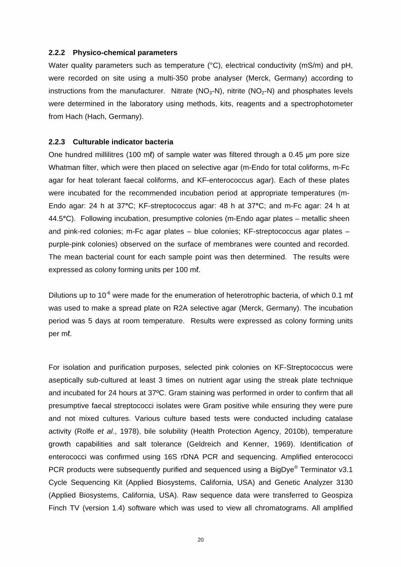
20

2.2.2 Physico-chemical parameters

Water quality parameters such as temperature (°C), electrical conductivity (mS/m) and pH,

were recorded on site using a multi-350 probe analyser (Merck, Germany) according to

instructions from the manufacturer. Nitrate (NO3-N), nitrite (NO2-N) and phosphates levels

were determined in the laboratory using methods, kits, reagents and a spectrophotometer

from Hach (Hach, Germany).

2.2.3 Culturable indicator bacteria

One hundred millilitres (100 mℓ) of sample water was filtered through a 0.45 μm pore size

Whatman filter, which were then placed on selective agar (m-Endo for total coliforms, m-Fc

agar for heat tolerant faecal coliforms, and KF-enterococcus agar). Each of these plates

were incubated for the recommended incubation period at appropriate temperatures (m-

Endo agar: 24 h at 37°C; KF-streptococcus agar: 48 h at 37°C; and m-Fc agar: 24 h at

44.5°C). Following incubation, presumptive colonies (m-Endo agar plates – metallic sheen

and pink-red colonies; m-Fc agar plates – blue colonies; KF-streptococcus agar plates –

purple-pink colonies) observed on the surface of membranes were counted and recorded.

The mean bacterial count for each sample point was then determined. The results were

expressed as colony forming units per 100 mℓ.

Dilutions up to 10-6 were made for the enumeration of heterotrophic bacteria, of which 0.1 mℓ

was used to make a spread plate on R2A selective agar (Merck, Germany). The incubation

period was 5 days at room temperature. Results were expressed as colony forming units

per mℓ.

For isolation and purification purposes, selected pink colonies on KF-Streptococcus were

aseptically sub-cultured at least 3 times on nutrient agar using the streak plate technique

and incubated for 24 hours at 37ºC. Gram staining was performed in order to confirm that all

presumptive faecal streptococci isolates were Gram positive while ensuring they were pure

and not mixed cultures. Various culture based tests were conducted including catalase

activity (Rolfe et al., 1978), bile solubility (Health Protection Agency, 2010b), temperature

growth capabilities and salt tolerance (Geldreich and Kenner, 1969). Identification of

enterococci was confirmed using 16S rDNA PCR and sequencing. Amplified enterococci

PCR products were subsequently purified and sequenced using a BigDye® Terminator v3.1

Cycle Sequencing Kit (Applied Biosystems, California, USA) and Genetic Analyzer 3130

(Applied Biosystems, California, USA). Raw sequence data were transferred to Geospiza

Finch TV (version 1.4) software which was used to view all chromatograms. All amplified

21

DNA sequences were identified using BLAST searches

(http://www.ncbi.nlm.nih.gov/BLAST). Consensus sequences were imported into Mega 5.0

(www.megasoftware.net) (Tamura et al., 2011) within which neighbour-joining trees were

constructed using the Jukes Cantor model and bootstrap values based on 1,000 replications

were selected (Tamura et al., 2011).

Antibiotic susceptibility tests were performed on enterococci isolates using the Kirby-Bauer

disk diffusion method according to Bauer et al. (1966). The overnight cultures were spread

onto Mueller Hinton agar (Merck, Germany) and these were allowed to dry. Antibiotics used

included: Ampicillin (10 µg), Amoxicillin (10 µg), Neomycin (30 µg), Streptomycin (300 µg),

Chloramphenicol (30 µg), Ciprofloxacin (5 µg), Oxy-tetracycline (30 µg), and Trimethoprim

(2.5 µg), Penicillin G (10 µg) and Vancomycin (30 µg) and were obtained from Mast

Diagnostics (UK). After incubation inhibition zones were measured in millimetres and

compared to the NCCLS growth inhibition zone standards for Streptococci (NCCLS, 1999).

2.2.4 Yeast

Yeast-malt-extract agar (YM) (10 g/ℓ glucose, 3 g/ℓ malt extract, 3 g/ℓ yeast extract, 5 g/ℓ

peptone and 15 g/ℓ agar) (Wickerham, 1951), supplemented with 100 ppm chloramphenicol

pH 5.5 was used for isolation of yeast. This was done using the membrane filter method

(APHA, 1988). Fifty millilitres of water was filtered through 0.45 µm HA membrane filters

(Whatman®). Each sample was analysed in duplicate. These membranes were then

placed onto YM agar plates, and incubated at 25°C. The formation of yeasts colonies were

examined daily during a 5 day period. Isolates were purified by sub culturing by streaking

onto YM agar (Wickerham, 1951).

The Diazonium blue B (Sigma-Aldrich, Germany) test was carried out to distinguish between

ascomycetous and basidiomycetous yeasts (Kurtzman & Fell, 1998). Isolates were further

identified using the ID 32C system (bioMerieux, France). The identities of the isolates were

confirmed by generating 26S rRNA sequencing data. A similar approach and methodology to

those used for the enterococci (Section 2.2.3) were used. Phylogenetic analysis was

performed with the MEGA version 5 software (Tamura et al., 2011). Statistical analysis was

based on the neighbour-joining method using bootstrap test of phylogeny (1000 replications)

and maximum composite likelihood model.

22

2.2.5 Molecular studies of microbial diversity

In this part of the study DNA was directly isolated from water samples. Water was filtered

through a 0.45 (and later through 0.22) μm filter and subsequently placed in a 1 mg/mℓ

lysozyme solution and glass beads. The filter was incubated at 37°C in a shaking water bath

for 10 min.

Proteinase K (1 mg/mℓ) was added and the solution still having the filter was incubated at

56°C for an additional 30 min. DNA was subsequently isolated from the crude lysate using

the PeqGold Bacterial DNA Kit (PEQLAB Biotechnologie GmbH, Erlangen, Germany). The

quality and quantity of the isolated nucleic acids were determined using the Nanodrop

ND1000 (NanoDrop Technologies, Delaware, USA) and agarose electrophoresis.

In the culture independent method PCR was performed directly using the community

genomic DNA. Denaturing gradient gel electrophoresis (DGGE) was conducted using

methods described by Muyzer et al., (1993). DNA bands were excised from DGGE gels with

a sterile scalpel blade, resuspended in twenty microlitres of nuclease-free water and

incubated overnight at 4°C. The eluate was then amplified using corresponding primer pairs

previously described (341F and 907R, Muyzer et al., 1993) without a GC-clamp. Amplified

PCR products were subsequently purified with the NucleoSpin Extract II Kit (Macherey-

Nagel GmbH, Dueren, Germany) and directly sequenced using a BigDye® Terminator

version 3.1 Cycle Sequencing Kit (Applied Biosystems, California, USA) and Genetic

Analyzer 3130 (Applied Biosystems, California, USA) as described in the manufacturer’s

instructions. Chromatograms were viewed in Geospiza Finch TV (version 1.4) software and

BLASTN searches (http://www.ncbi.nlm.nih.gov/BLAST) were used to determine the identity

of the amplified bands. The same sequencing approach was used in other Sections. DGGE

sequences were subsequently submitted to GenBank with accession numbers JQ085826-

JQ085849.

For NGS analysis the V1-V3 region of the 16S rRNA gene was amplified producing ~ 500 bp

fragments. The pyrosequencing sequencing analysis was contracted to Inqaba Biotech,

South Africa using the Roche 454 GS-FLXTM System. Sequences obtained from them were

trimmed to remove GS tags and further analysed with the CLC Bio Genomics Workbench

version 4.7.2 software (CLC Bio, Aarhus, Denmark). Sequences shorter than 200 bp in

length were excluded from data sets. All remaining sequences were subjected to the

National Center for Biotechnology Information (NCBI) database for BLAST analysis.

Sequences were then submitted to Pintail version 1.0 to detect the presence of PCR

artifacts. PCR products with chimeric properties were eliminated from data sets prior to

23

phylogenetic analysis. The remaining sequences were submitted to GenBank with accession

numbers JN865256-JN866178.

2.2.6 Enteroviruses and bacteriophages

a) Enteroviruses

Influent raw sewage (debris and grit already removed) and final effluent samples were

collected from three different waste water treatment plants in South Africa, namely

Potchefstroom (North West Province), Fochville and Carletonville (Gauteng province).

Influent samples were labelled CSW, FSW and PSW representing Carletonville, Fochville

and Potchefstroom respectively. Similarly, effluent samples were labelled CEF, FEF and

PEF for Carletonville, Fochville and Potchefstroom respectively (randomly numbered 1 to

and 3 not to identify the specific plant, results in Table 19 should not be associated with the

order of plant names presented here). Samples were immediately transferred on ice to the

laboratory for processing.

From November 2010 to September 2011, a total of 78 samples (13 influent and 13 effluent

samples from each of the three sites) were collected. A total volume of 2 ℓ wastewater

sample was collected at each instance.

Collected samples were processed immediately for virus recovery. The virus recovery

method used has been described previously by Nadan et al. (2003) and Meley et al. (2008).

Samples were replicated (n = 2) and named EF1 and EF2 for treated sewage and SW1 and

SW2 for untreated sewage. The samples were clarified by centrifugation using centrifuge

Harrier 18/8 for 30 min at 3,000 rpm. Each resultant pellet was resuspended in 10 mℓ of

supernatant fluid and clarified by addition of 10% (v/v) of chloroform.

The supernatant from first and second clarification procedures were pooled. The combined

supernatants were supplemented with 2.2% (W/v) NaCl and 7% (W/v) polyethylene glycol

6000. The mixture was stirred at 4°C overnight and then centrifuged for 2 h at 2,000 rpm at

4°C. The supernatant was discarded and the pellet was resuspended in lysis buffer of RNA

purification kit.

A two-step qRT-PCR was carried out. In the first stage, extracted RNA samples were

transcribed into cDNA using GoScript™ reverse transcription system. The resulting cDNA

templates were later used in the second stage for real time PCR (primer and probe

sequences are provided in Table 5). Standards were generated using known concentration

24

of enterovirus culture. The concentrations of the target enterovirus were quantified by using

the standard curves generated from known concentration of the enterovirus (Figure 16).

Table 5: Sequence details of the set of primers and probe used (Primers and Probe for amplification

of enterovirus were synthesised by Bioresearch Technologies, Inc.).

Primer Sequence Reference

Ev1 5'-GATTGTCACCATAAGCAGC-3' Fuhrman et al., 2005

Ev2 5'-CCCCTGAATGCGGCTAATC--3'

Probe 5'-FAM-CGGAACCGACTACTTTGGGTGTCCGT-BHQ-Phosphor-3'

b) Phage detection

i) Somatic coliphages

For isolation of somatic coliphages Escherichia coli strain C (ATCC 700078), also known as

WG5, a nalidixic acid-resistant mutant of ATCC 13706 was used (Green et al., 1999;

Ogorzaly and Ganzer, 2006). Into an microfuge tube 0.5 ml of the bacterial host and 1 ml of

a test sample (or an appropriate dilution if needed) was pipetted, the eppendorf tube was

then placed in an incubator at 37ºC for approximately 20-30 minutes for the phages to bind

to their host bacteria. This phage-host mixture was then poured into the test tube containing

the molten top agar (supplemented with naladixic acid) held at 50°C, mixed thoroughly and

then rapidly poured on top of the bottom agar. The top agar was allowed to solidify and dry

by opening the lids slightly. Once solidified and cooled, plates were incubated aerobically at

37°C for 18 hours. This procedure was carried out in duplicate.

ii) F-RNA phages

Salmonella enterica serovar Typhimurium WG 49 (ATCC 700730) was used as host in the

isolation of F-RNA phages. Processes were followed as described by Grabow, (2001) and

Mooijman et al. (2002). The host culture must be in a logarithmic, or log, phase of growth to

ensure the formation of the fertility-pili. To achieve this, an overnight culture is added to

Tryptone Soy Broth. The flask with bacterial culture is then placed in a shaking incubator for

2 to 4 hours at 37°C (100-150 rpm) and at intervals the absorbance is measured at a

wavelength 520 nm. At an absorbance approximately 0.5 the bacterial culture should be in

the logarithmic growth phase and is ready for use.

To top agar (2.5 ml; supplemented with naladixic acid) held at 50°C in a water bath, 1 ml of

premixed host and sample mixture was added, swirled to mix and poured onto the bottom

25

agar layer in a 90 mm petri dish. This was allowed to solidify and dry before inverted and

incubated overnight at 37°C.

2.2.7 Statistical analysis

The statistical analysis of all physico-chemical and microbiological parameters such as

standard deviation, minimum and maximum values were conducted in Statistica version 10

(StatSoft, US) and Microsoft Office Excel 2007. This data was a representation of three

replicates. Canoco (Canoco for Windows Version 4.0, GLW-CPRO ©) was used to create a

Redundancy Analysis (RDA) multivariate ordination diagram (Ter Braak, 1990). The RDA

was used to determine the relationship between dominant physico-chemical parameters and

bacterial or yeast species isolated from the respective surface water systems in 2010 and

2011. Data was log-transformed and significance tests were carried out using the Monte

Carlo permutation tests (499 permutations; p ≤ 0.05). All statistical analyses relationships

were considered to be statistically significant when the probability level was 0.05 or less

(≤0.05).

2.3 Results and Discussion

2.3.1 Physico-chemical parameters

The physico-chemical parameters for surface water measured in 2010 and 2011 were

generally within the Target Water Quality Ranges for domestic and recreational use.

Electrical conductivity (EC) for some of the sites was quite high which indicates potentially

some underlying quality challenges (Tables 7 and 8). The elevated EC levels were evident in

the sample sites associated with the Harts River (including Baberspan). These elevated EC

could be a sign of increasing salinity that could be a result of pollution.

26

Table 6: Physico-chemical parameters measured at each of the sampling sites at the respective

surface water source during 2010 sampling period. Highlighted values exceeded TWQR for domestic

use.

Water Source Sampling site

TWQR

pH

6-9

Temp (°C)

-

EC (mS/m)

0-70

NO3-N (mg/ℓ )

0-6 mg/ℓ

NO2-N (mg/ℓ )

0-6 mg/ℓ

PO42-

(mg/ℓ )

-

Mooi river Klerkskraal Dam 8.36 23.6 39 0.5 2 1.42

Muiskraal Dam 8.01 23.1 47 0.2 0 0.86

Around The World Bridge

7.76 23.0 70 0.6 4 0.68

Thabo Mbeki Drive 8.22 24.3 64 0.1 3 0.81

Trimpark North Bridge

8.25 24.6 65 0.4 3 0.02

Pedestrian Bridge 8.25 25.0 66 0.3 9 0.12

Viljoenroad Bridge 8.11 26.0 61 0.1 11 1.80

Harts river Dam 8 8.23 24.0 62 - - -

Jan Kempdorp 7.90 26.1 165 - 19 -

HRP Dam 7.10 24.1 135 3.5 2 1.70

Schoonspruit river

Orkney 7.61 21.7 52 1.7 3 2.44

Klerksdorp Bridge 7.74 22.5 39 - 2 0.41

Brakspruit 8.05 21.1 52 0.3 3 0.55

Bodenstein 7.91 20.4 60 0 4 0.63

Lower Vaal river

Windsorton 8.23 21.1 36 - 1 0

Barkley-Wes 8.47 19.3 40 - - 0

Schmidtsdrift 8.80 18.7 40 0.2 8 0

Christiana 7.86 19.0 36 0.4 4 0

Bloemhof 8.05 18.0 37 - 3 0

Barberspan Harts River 8.62 13.7 121 3.0 0.7 1.68

Inflow 8.58 15.2 115 4.0 - 1.02

Hotel 9.23 14.7 132 - - 0.11

Outflow 8.61 12.0 147 4.0 1.2 0.19

TWQR – target water quality range; Temp = temperature; EC = electrical conductivity; mS/m = milli siemens per

meter)

27

Table 7: Physico-chemical parameters measured at each of the sampling sites at the respective

surface water sources during 2011. Highlighted values exceeded TWQR for domestic use.

Water Source Sampling site

TWQR

pH

6-9

Temp (°C)

-

EC (mS/m)

0-70 mS/m

NO3-N (mg/ℓ )

0-6 mg/ℓ

NO2-N (mg/ℓ )

0-6 mg/ℓ

PO42- (mg/ℓ )

-

Harts river Spitskop Dam 8.25 16.4 84.3 - 2 0.44

Harts-Pampier Dam

8.28 15.4 133.1 1.0 4 0.33

Taung 7.95 11.8 47.9 0.3 3 0.43

Schweizer Reneke 8.33 13.7 78.8 0.1 4 0.34

Delareyville 8.75 13.1 109.6 0.4 4 0.70

Schoonspruit river

Orkney 7.88 18.9 51.2 - 3 0.33

Klerksdorp Bridge 7.85 18.9 43.2 0.1 2 0.86

Brakspruit 8.01 18.0 54.1 0.3 4 0.58

Bodenstein 7.92 17.0 64.4 0.8 3 1.03

Lower Vaal river

Windsorton 7.73 16.1 38.9 - - 0.10

Barkley-Wes 8.47 17.0 39.5 - 3 0.45

Schmidtsdrift 9.06 15.6 60.0 - 2 0.16

Christiana 9.08 11.2 40.1 - - -

Bloemhof 8.58 11.2 36.0 0.3 4 0.25

Barberspan and the upper Harts river

Harts River 7.92 22.4 47.1 0.8 5 1.74

Inflow 7.51 22.0 37.8 0.2 2 1.60

Hotel 8.75 22.6 99.8 0.2 1 -

Outflow 8.60 23.5 101.6 0.2 2 0.52

Sannieshof 7.58 23.6 45.4 0.1 3 2.19

Biesiesvlei 7.91 22.7 60.6 - 2 2.65

Lichtenburg 8.02 23.3 129.8 0.4 4 2.97

TWQR – target water quality range; Temp = temperature; EC = electrical conductivity; mS/m = milli siemens per

meter)

2.3.2 Levels of culturable indicator bacteria

Overall average total coliform, faecal coliform and E. coli levels were generally high at the

Lower Harts and Schoonspruit rivers while Barberspan had the lowest levels (Table 8). Low

28

levels of bacteria measured at Baberspan in 2010 may be due to the low water

temperatures. These samples were collected during winter. Sampling in 2011 was during the

warmer months and bacterial levels were considerably higher.

Total coliform, faecal coliform, E. coli and enterococci were present in all surface water

systems sampled. From Table 8 it is evident that except for the Schoonspruit, overall

average faecal coliform levels measured in surface water systems were generally within the

permissible TWQR for full (150 cfu/100 mℓ) and intermediate contact recreational (0-1000

cfu/100 mℓ) activities (DWAF, 1996).

Table 8: The microbiological water quality analysis of each sampling site within the 5 respective

surface water systems sampled in 2010 & 2011. TWQR for recreational use.

River system

TWQR

Sampling period

Total coliformscfu/100 mℓ

N/A

Faecal coliformscfu/100 mℓ

0-150

E. coli cfu/100 mℓ

0-130

Enterococcicfu/100 mℓ

0-30

Mooi Min Max

Ave±SD

2010

65.3 154.3

107.9±38.0

51.0 60.0

55.5±3.9

2.0

>17.0 9.2±5.2

17.3

147.0 47.1±47.0

Lower Harts Min Max

Ave±SD

2010

70.0

>300.0 192.5±173.2

20.6 242.0

131.0±126.5

22.0 76.0

49.0±38.2

44.0

287.3 165.8±117.8

Baberspan Min Max

Ave±SD

2010

4.0

270.0 80.0±127.1

6.0

130.0 36.7±62.5

0.0

33.6 9.6±16.1

36.0

127.3 68.7±40.5

Schoonspruit Min Max

Ave±SD

2010

252.6

>300.0 269.8±57.0

72.0 134.0

99.1±28.6

34.0 54.0

44.3±8.2

44.6 62.0

64.5±17.2 Vaal

Min Max

Ave±SD

2010

74.6

132.0 103.7±26.1

42.6 86.6

64.2±18.2

17.3 36.0

28.2±8.7

64.6

165.3 89.7±42.8

Lower Harts Min Max

Ave±SD 2011

26.0 >300.0

121.0±112.5

36.0 139.0

62.14±44.0

2.0 128.6.0

47.8±49.1

2.0 252.0

70.8±102.6Upper Harts & Baberspan

Min Max

Ave±SD

2011

156.0 >300.0

262.0±53.6

44.0 287.0

146.1±88.76

14.0 178.0

90.8±64.5

86.6 228.6

158.7±55.7 Schoonspruit

Min Max

Ave±SD

2011

202.3

>300.0 286.8±56.4

174.0

>300.0 279.8±70.5

91.3

>300.0 259.1.0±111.9

76.0

>300.0 250.3±116.6

Vaal Min Max

Ave±SD

2011

64.0 146.0

96.4±33.7

10.6

44.6.0 24.64. ±12.7

2.0

18.7 13.2±9.5

3.3 50.6

16.0.±20.4

TWQR – target water quality range; N/A – not applicable; cfu – colony forming unit; Min – minimum; Max –

maximum; Ave – average; SD – standard deviation

29

During the 2010 sampling period results indicated that Barberspan and the Schoonspruit

River had the highest overall average total coliform, faecal coliform, E. coli and enterococci

levels, while the Vaal River had the lowest levels. Total coliform and particularly faecal

coliform, E. coli and enterococci were also detected at all surface water systems during the

2011 sampling period. In this case Schoonspruit river was the only system with an overall

average faecal coliform level exceeding the TWQR for full contact recreational activities

(0-150 cfu/100 mℓ).

In 2010, enterococci levels measured at some of the sites in the Mooi River, Harts River,

Barberspan, Schoonspruit and Vaal Rivers exceeded the TWQR for full contact recreational

use. Enterococci levels exceeding the full contact recreational use TWQR were found at all

Barberspan and Schoonspruit sampling sites as well as some sites in the Harts and Vaal

Rivers. The acceptable TWQR for enterococci intermediate contact is 0-230 cfu/100 mℓ.

Some of the sites in the Harts River and Schoonspruit also exceeded this TWQR range.

The presence of enterococci that exceeded the TWQR for full contact use in these river

systems is of concern. This is because this water source is used for various water based

recreational as well as religious activities such as full body baptism, where the body is fully

submerged for brief periods. The lower body of the participants are in the water for extended

periods during the ceremony.

The biplots in Figures 5 and 6 represent the joint effect of environmental variables on the

levels of selected bacteria (Ter Braak, 1990). In these biplots the physico-chemical

parameters are represented by the thick red arrows and the species (bacterial faecal

indicators) by the thin blue arrows. The angle between the species (indicator bacteria) and

environmental variables reflect the influence on each other. A small angle indicates that a

strong correlation exists between data sets. An angle of 90° and larger indicates that there is

no correlation.

A positive correlation existed between levels of faecal coliform and E. coli. This is

demonstrated by the very small angles between these two variables in both Figures 5 and 6.

This type of relationship is expected since E. coli is a subgroup of faecal coliforms. Both

these figures further demonstrate that a positive correlation also existed between these

groups of bacteria (faecal coliforms and E. coli) on the one hand, and temperature and

phosphate levels on the other. A positive correlation also existed between enterococci and

total coliform levels measured in 2010. The same correlation was not seen with the 2011

data (Figure 6). However, in this biplot (Figure 6) a positive correlation between enterococci

30

on the one hand, and nitrate and TDS on the other hand is demonstrated. A positive

correlation also exists between the enterococci and nitrate levels. The same correlation was,

however, not observed in Figure 5.

Figure 5: Correlation biplot of 2010 data showing the relationship between dominant physico-

chemical parameters (pH, Temperature, TDS, EC, NO2-, NO3- and PO42-) and the levels of

enterococci, total coliforms, faecal coliforms and E. coli in 5 surface water sources. The physico-

chemical parameters are represented by red arrows, while the species are represented by blue

arrows.

-0.8 1.0

-0.6

0.6

Total coliforms

Faecal coliforms

E. coli

Faecal streptococciTemp

pH

EC

TDS

NO3-

NO2-

PO42-

SPECIES

ENV. VARIABLES

31

Figure 6: Correlation biplot of 2011 data illustrating the relationship between dominant physico-

chemical parameters (pH, Temperature, TDS, EC, NO2-, NO3

- and PO42-) and the prevalence of

enterococci, total coliforms, faecal coliforms and E. coli at 5 surface water sources. The physico-

chemical parameters are represented by red arrows, while the species are represented by blue

arrows.

2.3.3 Enterococcal species identification

Species identification was based on phenotypic and 16S rRNA sequence data. Table 9

below, presents a total of six species that were identified. These include Enterococcus

faecalis, E. faecium, E. mundtii, E. casseliflavus, E. gallinarum and E hirae. The most

frequently isolated species in 2010 were E. faecium (34%), E. casseliflavus (25%), and

E. mundtii (20%). Seventeen percent of the 2010 isolates were Enterococcus gallinarum.

-0.2 1.0

-1.0

Total coliforms

Faecal coliforms

E. coli

Faecal streptococci

Temp

pH

EC

TDS

NO3-

NO2-

PO42-

SPECIES

ENV. VARIABLES

32

The most frequently isolated species in 2011 were E. mundtii (37%), E. faecalis (33%) and

E. faecium (20%) E. casseliflavus, E. gallinarum and E hirae were less frequently isolated in

2011. Prevalence levels were 7% and below (Table 7). Enterococcus faecium was isolated

from all the water systems, for each sampling period in 2010 and 2011. Enterococcus

faecalis was only isolated in 2011.

Table 9: Number of Enterococci species identified in the samples from the various sites. Results are

provided for 2010 and 2011 sampling periods.

River System Year Enterococci species

E. faecalis

E. faecium

E. mundtii

E. casseliflavus

E. gallinarum

E. hirae

Mooi river 2010 8 1 1

Lower Harts

River 2010 1 1

2011 1 1 10 1 1

Barberspan &

Upper Harts 2010 1 7

2011 8 3 8

Schoonspruit 2010 1 2 3

2011 6 3 1 1

Vaal river 2010 1 6

2011 4 5 3 1

A neighbour-joining phylogenetic tree of enterococci species isolated from water systems in

2010 in provided in Figure 7. The tree is divided into 2 main clusters (A and B). Cluster A is

composed of 2 sub-clusters A1 and A2. Sub-cluster A1 is consists of E. mundtii and

E. faecium species whereas sub-cluster A2 is consists of E. faecium species. Furthermore,

in cluster B, E. casseliflavus and E. gallinarum species grouped into a single cluster. The

E. faecium group in cluster A is further grouped into 2 sub-clusters differentiated by distinct

branches. In this cluster grouping was according to species and strains but also according to

spatial distribution.

33

Figure 7: Neighbour-joining (N-J) tree showing the phylogenetic relationships of 35 enterococci

species isolated from the 5 surface water systems in 2010. The Jukes Cantor model was used to

generate the N-J tree. Bootstrap percentages are indicated at the branching points of the

dendrogram.

The neighbour-joining phylogenetic tree of enterococci species isolated from 5 surface water

systems during 2011 is depicted in Figure 8. This tree was similar to the 2010 tree depicted

in Figure 7. In Figure 8 there are also 3 main clusters, A and B. Cluster A is composed of 3

10.9 Enterococcus mundtii Aq5

10.11 Enterococcus mundtii Aq5

10.6 Enterococcus mundtii Aq5 10.4 Enterococcus mundtii Aq5 10.8 Enterococcus mundtii Aq5 10.7 Enterococcus mundtii Aq5 10.1 Enterococcus mundtii Aq5 38 Enterococcus hirae M10_2A 4.2 Enterococcus faecium SJL302

4.6 Enterococcus faecium 044

4.8 Enterococcus faecium 044

4.3 Enterococcus faecium SJL302

A1

8.9 Enterococcus faecium CE3.A

4.1 Enterococcus faecium CE3.A

10.10 Enterococcus faecium CE3.A

6.1 Enterococcus faecium CE3.A

1.4 Enterococcus faecium CE3.A

4.16 Enterococcus faecium CE3.A

4.17 Enterococcus faecium CE3.A

5.6 Enterococcus faecium CE3.A

A2

6.6 Enterococcus casseliflavus RZC110

8.5 Enterococcus casseliflavus RZC110

6.3 Enterococcus casseliflavus RZC110

8.7 Enterococcus casseliflavus RZC110 8.8 Enterococcus casseliflavus RZC110 8.3 Enterococcus casseliflavus LHICA_41_ 6 8.6 Enterococcus casseliflavus LHICA_41_6 8.4 Enterococcus casseliflavus LHICA_41_6

5.1 Enterococcus gallinarum W184

5.3 Enterococcus gallinarum W184

4.9 Enterococcus casseliflavus LHICA_41_6

5.2 Enterococcus gallinarum W184

6.11 Enterococcus gallinarum W184 6.9 Enterococcus gallinarum W184

6.12 Enterococcus gallinarum U82

B1

66

66

59

66

52100

67

66

58

81

99

56

55

53

78

98

99

0.002 Sequence similarity (%)

A

B

34

sub-clusters A1, A2 and A3. These are species specific consisting of Enterococcus mundtii

(A1), E. faecium (A2) and E. casseliflavus (A3). The A1 and A2 subclusters are supported

by a 99% bootstrap. Cluster B is composed of the E. faecalis group. The individual isolates

from the E. mundtii group is closely related to strain Aq5 sequences that were available on

GenBank. These E. mundtii species were isolated from the Lower Harts River and

Barberspan.

The E. faecalis species was first identified in the 2011 surface water samples. This group

was predominantly isolated from the Upper Harts and Schoonspruit rivers. The E. faecalis

group is divided into two subgroups at the interspecies level and the relatedness of these

species is supported by an 88% bootstrap confidence. The sequences from two strains in

GenBank (E12 and UGRA10) were identified in this species group.

35

Figure 8: Neighbour-joining graph showing the phylogenetic relationships of 56 enterococci species

isolated from 5 surface water systems in 2011 according to the Jukes Cantor model. Bootstrap

percentages are indicated at the branching points of the dendrogram.

13.14 Enterococcus mundtii Aq5

14.6 Enterococcus mundtii Aq5

14.9 Enterococcus mundtii Aq5

13.12 Enterococcus mundtii Aq5

14.2 Enterococcus mundtii Aq5

14.4 Enterococcus mundtii Aq5

14.3 Enterococcus mundtii Aq5

14.12 Enterococcus mundtii Aq5

14.10 Enterococcus mundtii Aq5

11.7 Enterococcus mundtii Aq5

14.5 Enterococcus mundtii Aq5

13.4 Enterococcus mundtii Aq5

11.2 Enterococcus mundtii Aq5

14.1 Enterococcus mundtii Aq5

14.11 Enterococcus mundtii Aq5

11.9 Enterococcus mundtii Aq5

11.8 Enterococcus mundtii Aq5

11.11 Enterococcus mundtii Aq5

11.21 Enterococcus mundtii HAMB 13965

11.10 Enterococcus mundtii Aq5 11.12 Enterococcus mundtii Aq5

A1

13.7 Enterococcus faecium SJL302

11.16 Enterococcus faecium SJL302

13.11 Enterococcus faecium SJL302

11.4 Enterococcus faecium SJL302

12.2 Enterococcus faecium SJL302

13.10 Enterococcus faecium 044

12.4 Enterococcus faecium 004

12.1 Enterococcus faecium 004

14.7 Enterococcus faecium 044

11.1 Enterococcus faecium SJL302

12.5 Enterococcus faecium 0104

13.5 Enterococcus faecium 044

13.6 Enterococcus faecium 044

A2

13.9 Enterococcus casseliflavus LHICA_41_6

14.14 Enterococcus gallinarum UPAA106

12.9 Enterococcus casseliflavus RZC110

14.13 Enterococcus casseliflavus RZC110

A3

11.13 Enterococcus faecalis E12 11.18 Enterococcus faecalis E12

11.3 Enterococcus faecalis E12

11.5 Enterococcus faecalis E12

11.19 Enterococcus faecalis E12

12.10 Enterococcus faecalis E12

12.7 Enterococcus faecalis E12

13.1 Enterococcus faecalis E12

11.17 Enterococcus faecalis E12

12.3 Enterococcus faecalis E12

13.13 Enterococcus faecalis E12

14.8 Enterococcus faecalis E12

12.6 Enterococcus faecalis E12

12.8 Enterococcus faecalis E12

11.14 Enterococcus faecalis E12

13.3 Enterococcus faecalis E12

12.11 Enterococcus faecalis E12

13.2 Enterococcus faecalis E12

B1

86

60

54

99

65

62

60

95

63

58

74

99

99

89

0.002 Sequence similarities (%)

A

B

36

2.3.4 Levels and diversity of yeasts

The average yeast numbers, statistical differences in pigmented and non-pigmented yeasts

between sites and their percentage detected at the sites are presented in Tables 8 and 9.

The physico-chemical parameters listed in Tables 5 and 6 are also relevant for the levels of

yeast. Sampling was done on the same days when sampling for enterococci was done.

When the values of Tables 8 and 9 are compared to the physico-chemical data in Tables 5

and 6 it is evident that the non-pigmented yeast numbers were higher when the water

temperature was elevated. This was expected as yeast generally preferred warmer

temperatures.

Overall comparison of the total number of pigmented and non-pigmented yeasts shows that

the latter were detected in a much higher levels. In 2010, the highest number of pigmented

yeasts was found among the Schoonspruit river samples (e.g. Klerksdorp Bridge, 1066

cfu/L). Tukey’s HSD statistics revealed significant differences in pigmented yeast numbers

between different sites but no significant differences in non-pigmented yeasts (Tables 8 and

9). Pigmented yeast levels in the Schoonspruit River were significantly higher (P< 0.05)

than in all the other water sources.

The results were analysed by Canoco software (Ter Braak, 1990). Figure 9 is a redundancy

analysis diagram showing the correlations between the environmental parameters and levels

of yeasts. Results obtained by RDA analysis indicated a positive correlation between the

pigmented yeasts and phosphates (Figure 9). It also indicated that a positive correlation

existed between Orkney, Klerkskraal Dam and Viljoen Road Bridge sites on the one hand,

and phosphates on the other. The non-pigmented yeasts had a positive correlation with

temperature. Furthermore, a positive correlation also existed between the yeast levels at

Around the World bridge and Thabo Mbeki drive sites on the one hand, and temperature on

the other. The other two environmental parameters (TDS and NO2-N) however, did not have

any correlation with the pigmented or non-pigmented yeast levels

37

Figure 9: Redundancy analysis (RDA) diagram illustrating the correlation between environmental

variables and species (pigmented and non-pigmented yeasts) measured in 2010. The red vectors

represent the environmental parameters and blue vectors the species (pigmented and non-pigmented

yeasts). Eigenvalues for the first two axes were 0.115 and 0.032 respectively.

-1.0 1.0

-1.0

1.0

Pigmented

Non-pigmentedTemp

TDS NO2

PO4

BB_HR

BB_inf

BB_H

BB_out

MR_KD

MR_MK

MR_ATWB

MR_TMD

MR_TP

MR_PB

MR_VRB

VR_BHD

VR_Chr

VR_WN

VR_BW

VR_SD

SS_Ork

SS_KDB

SS_BS

SS_Bond

HR_Dam8

HR_JKDHR_HR

SPECIES

ENV. VARIABLES

SAMPLES

Barberspan Mooi River Vaal River Schoonspruit River Harts River

38

Table 10: Average yeast numbers (cfu/ℓ) at various water sources of different sites indicating

pigmented and non-pigmented yeasts distribution of 2010.

Water Source Sites Ave±SD (cfu/ℓ) 1,2 Percentage (%)3

Mooi river Klerkskraal Dam Pigmented 73.0±64.0a, b 2.3

Non-pigmented

3070.0±1930.0a 97.7

Muiskraal Bridge Pigmented 210.0±93.0a, b, c 42.5

Non-pigmented

280.0±23.0a 57.5

Around The World Bridge

Pigmented 0.0a 0

Non-pigmented

8680.0±7810.0a 100

Thabo Mbeki drivePigmented 0.0a 0

Non-pigmented

473.0±154.0a 100

Trimpark North Bridge

Pigmented 0.0a 4.4

Non-pigmented

2270.0±1920.0a 95.6

Pedestrian Bridge Pigmented 0.0a 0

Non-pigmented

0.0a 0

Viljoenroad Bridge Pigmented 0.0a 0

Non-pigmented

1000.0±580.0a 100

Lower Harts river Dam 8 Pigmented 0.0a 0

Non-pigmented

16.0±4.0a 100

Jan Kempdorp Pigmented 2.0±0.3a 66.7

Non-pigmented

1.0±0.6a 33.3

HRP Dam Pigmented 0.0a 0

Non-pigmented

33.0±9.0a 100

Schoonspruit

Orkney Pigmented 646.0±26.6d 58.0

Non-pigmented

466.7±145.3a 42.0

Klerksdorp Bridge Pigmented 1066.0±67.0e 72.7 Non-

pigmented 400.0±28.9a 27.3

Brakspruit Pigmented 430.0±190.0c, d 73.8 Non-

pigmented 150.0±55.0a 26.1

Bodenstein Pigmented 300.0±12.0b, c 100 Non-

pigmented 0.0a 0

Vaal river Windsorton Pigmented 0.0a, b 0

Non-

pigmented 35.0±5.0a 100

Barkley-Wes Pigmented 0.0a, b 0

39

Water Source Sites Ave±SD (cfu/ℓ) 1,2 Percentage (%)3

Non-

pigmented 10.0±5.0a 100

Schmidtsdrift Pigmented 10.0±2.0a, b 7.5

Non-

pigmented 120.0±2.5a 92.5

Christiana Pigmented 0.0a, b 0

Non-

pigmented 47.0±7.0a 100

Baberspan Harts River (Town)

Pigmented 20.0±20.0a, b 41.0

Non-

pigmented 10.0±10.0a 59.0

Inflow Pigmented 45.0±15.0a, b 52.9

Non-

pigmented 40.0±40.0a 47.1

Hotel Pigmented 0.0a, b 0

Non-

pigmented 5.0±5.0a 100

Outflow Pigmented 10.0a, b 40.0

Non-pigmented

15.0±5.0a 60.0

1Values given are average values at each sampled site (Ave) ± standard deviation (SD). 2Sites with the same combination of superscript alphabetic letters a,b,c,d indicate no significant differences (P> 0.05) among sites, while those with different letters indicate significant differences at P< 0.05 (Tukey’s HSD). 3Percentage pigmented and non-pigmented yeasts Table 11: Average yeast numbers (cfu/ℓ) at various water sources of different sites indicating

pigmented and non-pigmented yeasts distribution of 2011.

Water Source Sites Ave±SD (cfu/ℓ) 1,2 Percentage (%)3

Upper Harts river

Spitskop Dam Pigmented 0.0a 0

Non-pigmented

4120.0±200.0a 100

Harts-Pampier Dam

Pigmented 1310.0±270.0b 51.6

Non-pigmented

1230.0±50.0a 48.4

Taung Pigmented 180.0±80.0a 0.1

Non-

pigmented 17200.0±1760.0c, d 99

Schweizer Reineke

Pigmented 60.0a 0.4

Non-pigmented

16120.0±920.0c 99.6

Delareyville Pigmented 30.0±10.0a 0.6

Non-

pigmented 4590.0±190.0a, b 99.4

Schoonspruit Orkney Pigmented 3760.0±400.0c 13.9

Non-

pigmented 23240.0±1960.0c, d 86.1

40

Water Source Sites Ave±SD (cfu/ℓ) 1,2 Percentage (%)3

Klerksdorp Bridge

Pigmented 100.0±20.0a 0.4

Non-pigmented

28280.0±520.0d 99.6

Brakspruit Pigmented 130.0±110.0a 0.8

Non-

pigmented 16040.0±8200.0b, c 99.2

Bodenstein Pigmented 10.0±10.0a 1.4

Non-

pigmented 730.0±310.0a 98.6

Vaal river Windsorton Pigmented 40.0±20.0a 17.4

Non-

pigmented 190.0±50.0a 82.6

Barkley-Wes Pigmented 0.0a 0

Non-

pigmented 1830.0±1770.0a 100

Schmidtsdrift Pigmented 0.0a 0

Non-

pigmented 4180.0±2260.0a 100

Christiana Pigmented 280.0±120.0a 31.1

Non-

pigmented 620.0±140.0a 68.9

Bloemhof Dam Pigmented 20.0±20.0a 1.7

Non-

pigmented 1150.0±250.0a 98.3

Upper Harts river and

Baberspan

Harts River (Town)

Pigmented 230.0±150.0a 33.8

Non-

pigmented 450.0±50.0a 66.2

Inflow Pigmented 1180.0±160.0b 43.4

Non-

pigmented 1540.0±120.0a 56.6

Hotel Pigmented 50.0±10.0a 18.5

Non-

pigmented 220.0±20.0a 81.5

Outflow Pigmented 400.0±80.0a 18.0

Non-

pigmented 1820.0±120.0a 82.0

Sannieshof Pigmented 50.0±10.0a 3.3

Non-

pigmented 1450.0±250.0a 96.7

Biesiesvlei Pigmented 10.0±10.0a 0.3

Non-

pigmented 2960.0±560.0a 99.7

Lichtenburg Pigmented 110.0±90.0a 5.8

Non-pigmented

1800.0±400.0a 94.2 1Values given are average values at each sampled site (Ave) ± standard deviation (SD). 2Sites with the same combination of superscript alphabetic letters a,b,c,d indicate no significant differences (P> 0.05) among sites, while those with different letters indicate significant differences at P< 0.05 (Tukey’s HSD). 3Percentage pigmented and non-pigmented yeasts.

41

During the 2011 sampling significant differences were also found when pigmented and non-

pigmented yeasts levels between sites were compared (Table 8). The only significant

differences in pigmented yeast levels were observed between Harts Pampierstad Bridge,

Baberspan Inflow and the Orkney sites. Pigmented yeast levels in the Schoonspruit River

were again higher (P< 0.05) than in all the other water sources. In Section 2.3.2 it was also

demonstrated that the enterococci levels at Schoonspruit was on average higher than the

other sampling points.

The 2011 results were also analysed by Canoco software (Ter Braak, 1990). Figure 10 is a

redundancy analysis diagram showing the correlations between the environmental

parameters and levels of yeasts.

Figure 10: Redundancy analysis (RDA) diagram illustrating the correlation between environmental

variables and species (pigmented and non-pigmented yeasts) measured in 2011. The red vectors

represent the environmental parameters and blue vectors the species (pigmented and non-pigmented

yeasts). Eigenvalues for the first two axes were 0.107 and 0.025 respectively.

RDA analysis indicated a positive correlation existed between the levels of non-pigmented

yeasts and nitrate (Figure 10). It also indicated that yeast levels measured at Barkley-Wes

and Schweizer Reineke were correlated to nitrate levels. The rest of the environmental

-1.0 1.0

-1.0

1.0

pigm

non_pigm

Temp

TDS

NO2

PO4BB_HRBB_inf

BB_H BB_out

BB_SH

BB_BV

BB_LB

VR_BHD

VR_Chr

VR_WNVR_BW VR_SD

SS_Ork

SS_KDBSS_BS

SS_Bond

HR_SDam

HR_HR

HR_Tau

HR_SWRHR_DVH

SPECIES

ENV. VARIABLES

SAMPLES

Barberspan Vaal River Schoonspruit River Harts River

42

parameters, however, did not have any correlation with the pigmented or non-pigmented

yeasts or the levels of yeast at the specific sites.

Results in Table 10 are further summarised in Table 12 and results of Table 11 summarised

in Table 13. These tables indicate that a large number of yeasts were isolated but also that

the distribution of the various yeasts was not uniform.

Table 12: Percentage ascomycetous and basidiomycetous yeasts from the North West Province

during 2010.

Surface water sources

% Ascomycetous yeasts

% Basidiomycetous Yeasts

% Pigmented

% non- Pigmented

Mooi river (n=23)

85 - - 100 - 15 5 -

Harts river (n=17)

95 - - 100 - 5 0 -

Schoonspruit river

(n=25)

28 - - 100 - 72 56 44

Lower Vaal river (n=25)

61 - - 100 - 39 92 8

Barberspan (n=13)

8 - - 100 - 92 38 62

Table 13: Percentage ascomycetous and basidiomycetous yeasts from the North West Province

during 2011.

Surface water sources

% Ascomycetous yeasts

% Basidiomycetous Yeasts

% Pigmented

% non-

Pigmented

Harts river (n=22)

50 - - 100 - 50 32 18

Schoonspruit River

(n=22)

64 - - 100 - 36 27 9

Lower Vaal river (n=18)

83 - - 100 - 17 17 6

Barberspan (n=26)

50 - - 100 - 50 38 12

All ascomycetous and basidiomycetous yeasts from the respective water sources were able

to grow at 25°C (Table 14). This was expected since all these yeasts were isolated at this

temperature. However, a large percentage of the isolates were able to grow at 37°C and

higher temperatures. Determining the ability of yeasts to grow at 37°C may be important as

this temperature is associated with warm-blooded animals. Human opportunistic pathogenic

yeasts are known to thrive at this temperature. Typically such species include Candida

43

albicans and Candida tropicalis and a number of other opportunistic pathogenic yeasts

(Medeiros et al., 2008). Results also indicated that isolates from the respective surface

water sources can grow at a minimum temperature of 4°C (psycrophylic) and at the

maximum temperature used in this study (40°C; thermo-tolerant).

Table 14: Percentage ascomycetous and basidiomycetous yeasts growing at various temperatures.

Surface water sources

% of isolates that grew at

4°C 25°C 30°C 37°C 40°C

Harts river (n=22)

Ascomycetous 68 100 68 64 70

Basidiomycetous 32 100 32 36 25

Schoonspruit river

(n=22)

Ascomycetous 100 100 100 18 0

Basidiomycetous 100 100 100 0 0

Lower Vaal river (n=18)

Ascomycetous 83 100 83 50 33

Basidiomycetous 17 100 17 11 6

Barberspan (n=26)

Ascomycetous 42 100 42 27 38

Basidiomycetous 50 100 50 19 38

2.3.5 Phenotypic and genetic identification of yeasts

The morphological characteristics were determined by microscopy. Figure 11 shows

photographs of selected isolates indicating the morphological appearance. The cells were

spheroidal or ovoidal. Yeast colonies were cream to tan or pink colour, with a smooth

texture.

44

Figure 11: Photograph of some of the isolated yeasts (400X magnification)

Biochemical identification of the yeasts indicated that Candida spp. were the most prevalent,

followed by Rhodotorula spp., Wickerhamomyces spp., Pichia spp., Clavispora spp.,

Cryptococcus spp., Sporidiobolus spp., Hanseniaspora spp., Cystofilbasidium spp.,

Meyerozyma spp., Aureobasidium spp. and Saccharamyces spp.. Identities of these species

were confirmed using D1/D2 region of the 26S rRNA gene sequence data. These sequence

data were analysed by MEGA 5 software and the resulting neighbour joining tree for the

2010 sampling period is provided in Figure 12 and those of the 2011 period in Figure 13.

45

Figure 12: Neighbour-joining tree based on partial sequences of D1/D2 domain of 26S rDNA

obtained in 2010. The tree was constructed using the Kimura two-parameter method. Local

bootstrap probability values obtained by maximum likelihood analysis are indicated at the branche

nodes.

HOTEL2WIT NL-1

79 NL 1

95 NL 1

Wickerhamomyces anomalus

Candida boidinii 86 NL 1

Candida temnochilae HW-1 NL-1

Candida tropicalis 85 NL 1

Candida nivariensis JW-1 NL1

19 NL 1

21 NL 1Candida pseudolambica

JW-2 NL-1

22 NL 1

32 NL 1

Pichia kudriavzevii

89 NL 1

C NL 1Clavispora lusitaniae

Ascomycetous yeasts

Rhodotorula slooffiae JW-3 NL-1

Sporidiobolus pararoseus HR NL-1

OUTPINK NL-1

G NL 1

B NL 1

D NL 1

Rhodotorula glutinis

F NL 1

28 NL 1

yv1 NL 1

96 NL 1

HOTEL1PINK NL-1

A NL 1

Rhodotorula mucilaginosa

Basidiomycetous yeasts

100

100

99

100

100

58

100

76

51

71

53

52

100

79

65

91

99

100

73

67

64

98

66

0.05

46

Figure 13: Neighbour-joining tree based on partial sequences of D1/D2 domain of 26S rDNA

obtained in 2010. The tree was constructed using the Kimura two-parameter method. Local

bootstrap probability values obtained by maximum likelihood analysis are indicated at the branche

nodes.

SW1 pink NL 1

Brak1 pink NL 1(2)

LIG2P NL-1

OUTPINK NL-1

Rhodotorula glutinis

Rhodotorula sp. CP1 NL-1

BIES1PINK NL-1

Ork2 pink NL-1

HOTEL1PINK NL-1

Tg2 pink NL-1

D1 pink NL-1

Rhodotorula mucilaginosa

Sporidiobolus pararoseus HR NL-1

Rhodotorula slooffiae HP2 pink NL-1

Cystofilobasidium sp. WW-2 NL-1

IF 1 NL 1

SW2 wit NL 1Cryptococcus flavescens

Cryptococcus albidosimilis Out wit 2 NL 1

Klerk1 orange NL-1

Klerk2 wit2 NL-1Cryptococcus diffluens

Basidiomycetous yeasts

BIESWIT NL-1

BW-3 NL-1

Tg1 wit NL-1

Candida intermedia

Klerk2 wit1 NL 1

Brak1 wit3 NL 1(2)Clavispora lustaniae

BW1-1 NL-1

Brak2 wit3 NL 1

Bod2 wit1 NL 1

Candida pseudolambica

Pichia kudriavzevii SpD1 wit NL-1

Pichia sp. CW 2 NL 1

SW4 NL-1

WW-1 NL-1Hanseniaspora uvarum

Candida navariensis SpD2 wit NL1

Saccharomyces sp. SAN2W NL-1

Ork1 wit2 NL-1

Ork2 wit2 NL-1Candida glaebosa

Meyerozyma guilliermondii LIG2WIT NL-1

Candida temnochilae HP1 wit NL-1

Meyerozyma guilliermondii WP-1 NL-1

WW-3 NL-1

BW-1 NL-1

HOTEL2WIT NL-1

Wickerhamomyces anomalus

Ascomycetous yeasts

75

100

100

100

100

100

100

97

99

72

75

70

55

82

63

62

86

48

65

90

98

94

56

100

82

99

73

73

99

54

98

84

69

69

0.05

47

The ascomycedious and basidiomycetous yeast formed separate clusters in both

phyogenetic trees (Figures 12 and 13). Ascomycetous yeasts consisted mainly of

Wickerhamomyces sp., Candida sp., Pichia sp. and Clavispora sp. The basidiomycetous

yeast group was made up of Rhodotorula sp. and Sporidiobolis sp. In 2011 similar groupings

were observed in the neighbour-joining tree. However, in this case there was a greater

diversity of both basio- and ascomycetous yeasts. Cryptococcus sp. as well as

Cystofilobasidium sp. were present among the basidiomycetous yeasts. Amongst the

ascomycetous yeasts Hanseniaspora sp., Saccharomyces sp., and Meyerozyma sp. were

also isolated (Figure 13).

2.3.6 Molecular studies of microbial diversity

Denaturing gradient gel electrophoresis (DGGE) as well as high throughput sequencing

(HTS) or metagenomic sequencing was used to determine the diversity of bacterial species

in some surface water sources. DGGE banding profiles of the bacterial diversity for the

winter and summer season are depicted in Figure 14.

Figure 14: DGGE bacterial community analyses for surface water in winter and summer at the Vaal

river sampling sites, Deneysville (D), Parys (P), Scandinawieë Drift (SD) and Barrage (B). Indicator

species included were E. coli (E.c), Pseudomonas aeruginosa (P.a), Streptococcus faecalis (S.f) and

Staphylococcus aureus (S.a).

48

DGGE profiles demonstrated high resolution and intensity at a denaturing gradient of

30–60%. Several bands were observed in the DGGE profiles. Four bacterial species,

Escherichia coli, Pseudomonas aeruginosa, Streptococcus feacalis and Staphylococcus

aureus, were included in DGGE gels to determine the potential of using such an approach to

establish the presence of these species in water samples. Corresponding bands for

Staphylococcus aureus and Pseudomonas aeruginosa were observed for Parys,

Scandinawieë Drift and Vaal Barrage. In addition, Parys had a band with similar migration

patterns to Escherichia coli. The corresponding bands were excised and sequenced but

produced poor quality sequences with indefinite identification. Since sequence data could

not confirm accurate identification of the excised bands, results remain inconclusive. Bands

with similar migration patterns for Streptococcus feacalis were not observed in DGGE

profiles (Figure 14).

Spatial and temporal changes in the bacterial community composition among the four

sampling sites were evident (Figure 14). DGGE profiles yielded several distinct bands

representing the structure of the numerically dominant bacterial population at the time of

sampling. There were a large number of faint bands that were visible in the gels that could

potentially indicate community complexity. Dominant bands present at Vaal Barrage, Parys

and Scandinawieë Drift displayed similar migration patterns that may indicate the distribution

of potentially related and dominant bacterial species between the three sampling points. In

contrast, Deneysville illustrated a distinctive bacterial diversity compared to the three other

sites. In this case (Deneysville sample), a small number of dominant bands exhibited similar

migration patterns to Parys, Scandinawieë Drift and Vaal Barrage. Similar banding patterns

of dominant bands may suggest the growth and reproduction of a few dominant species at

the Deneysville sampling site, compared to the downstream sampling sites (Parys,

Scandinawieë Drift and Vaal Barrage)

Dominant bands across all sampling sites were excised, re-amplified and sequenced.

Sequence quality for the DGGE bands was generally sufficient for identification.

Identification details are provided in Table 15. Phylogenetic groups present during the winter

and summer season included Cyanobacteria, Bacteroidetes and Betaproteobacteria.

However, bacterial community compositions for the four sampling stations shifted during

seasonal changes. Community composition for Deneysville mainly consisted of

Betaproteobacteria during the winter season, whereas Cyanobacteria dominated during the

summer season. The high abundance of Cyanobacteria during summer may be associated

with the green algal blooms observed at the time of sampling. Vaal Barrage, Parys and

Scandinawieë Drift consisted primarily of Bacteroidetes and Cyanobacteria during winter, but

49

shifted in community composition during summer so that Bacteroidetes and

Betaproteobacteria were dominant at all three sites.

50

Tab

le 1

5: S

eque

nce

iden

tific

atio

n of

PC

R-D

GG

E b

ands

usi

ng r

efer

ence

seq

uenc

es in

the

NC

BI d

atab

ase.

DG

GE

ban

d n

o.

NC

BI a

cces

sio

n

no

.

Clo

sest

rel

ativ

e (a

cces

sio

n n

o.)

P

hyl

og

enet

ic a

ffili

atio

nP

erce

nta

ge

(%)

sim

ilari

ty

B1

JQ08

5826

U

ncul

ture

d ba

cter

ium

clo

ne X

YH

PA

.091

2.16

0 (H

Q90

4787

) B

acte

ria

100

B2

JQ08

5827

U

ncul

ture

d M

ethy

loph

ilace

ae b

acte

rium

clo

ne Y

L203

(H

M85

6564

) B

eta

prot

eoba

cter

ia

100

B3

JQ08

5828

U

ncul

ture

d ba

cter

ium

clo

ne S

W-O

ct-1

07 (

HQ

2038

12)

Bac

teria

10

0

B4

JQ08

5829

U

ncul

ture

d C

yano

bact

eriu

m c

lone

TH

_g80

(E

U98

0259

) C

yano

bact

eria

10

0

B5

JQ08

5830

U

ncul

ture

d ba

cter

ium

clo

ne S

INO

976

(HM

1300

28)

Bac

teria

99

B6

JQ08

5831

U

ncul

ture

d H

alis

com

enob

acte

r sp

. clo

ne W

R41

(H

M20

8523

) B

acte

roid

etes

96

B7

JQ08

5832

U

ncul

ture

d ba

cter

ium

clo

ne M

cSIP

B07

(F

J604

747)

B

acte

ria

98

B8

JQ08

5833

U

ncul

ture

d ba

cter

ium

clo

ne E

S3-

64 (

DQ

4632

83)

Bac

teria

99

B9

JQ08

5834

U

ncul

ture

d ba

cter

ium

clo

ne A

NT

31 (

HQ

0152

63)

Bac

teria

10

0

B10

JQ

0858

35

Unc

ultu

red

bact

eriu

m c

lone

SIN

G42

3 (H

M12

9081

) B

acte

ria

99

B11

JQ

0858

36

Unc

ultu

red

Bac

tero

idet

es s

p. c

lone

MA

161E

10 (

FJ5

3286

4)

Bac

tero

idet

es

100

B12

JQ

0858

37

Unc

ultu

red

Nitr

osom

onad

acea

e b

acte

rium

clo

ne Y

L004

(H

M85

6379

)B

eta

prot

eoba

cter

ia

92

B13

JQ

0858

38

Aph

aniz

omen

on g

raci

le A

CC

S 1

11 (

HQ

7008

36)

Cya

noba

cter

ia

91

B14

JQ

0858

39

Ana

baen

a ci

rcin

alis

LM

EC

YA

123

(E

U07

859)

C

yano

bact

eria

97

B15

JQ

0858

40

Cym

bella

Hel

vetic

a s

trai

n N

JCH

73 (

JF27

7135

) C

yano

bact

eria

99

B16

JQ

0858

41

Unc

ultu

red

bact

eriu

m c

lone

Frs

Fi2

08 (

JF74

7973

) B

acte

ria

99

B17

JQ

0858

42

Unc

ultu

red

Cya

noba

cter

ium

clo

ne L

iUU

-11-

80 (

HQ

3866

09)

Cya

noba

cter

ia

98

B18

JQ

0858

43

Unc

ultu

red

bact

eriu

m c

lone

TG

-FD

-0.7

-May

-09-

B06

1 (H

Q53

2969

) B

acte

ria

99

B19

JQ

0858

44

Unc

ultu

red

bact

eriu

m c

lone

C_J

97 (

EU

7357

34)

Bac

teria

89

B20

JQ

0858

45

U

ncul

ture

d ba

cter

ium

clo

ne L

c2yS

22-M

L-05

6 (F

J355

035)

Bac

teria

97

B21

JQ

0858

46

Unc

ultu

red

bact

eriu

m c

lone

ncd

240a

07c1

(H

M26

8907

) B

acte

ria

91

B22

JQ

0858

47

Unc

ultu

red

Sph

ingo

bact

eriu

m s

p. H

aLB

8 (H

M35

2374

) B

acte

roid

etes

10

0

B23

JQ

0858

48

Unc

ultu

red

Cya

noba

cter

ium

isol

ate

DG

GE

gel

ban

d B

5 (J

N37

7930

) C

yano

bact

eria

98

B24

JQ

0858

49

Unc

ultu

red

Dec

hlor

osom

a sp

. clo

ne M

BfR

-NS

P-1

59 (

JN12

5313

) B

eta

prot

eoba

cter

ia

86

The sam

16S rRN

sites. T

me DNA sa

NA. A total

his data we

amples wer

of eighteen

ere analysed

re subjected

n phylogene

d and are p

51

d to high th

etic groups

provided in F

hrough put

were ident

Figure 15 (A

sequencing

tified among

A-F).

g (HTS) ana

g the four s

alysis of

sampling

Figure 1

the Vaa

Deneysv

Scandin

Betapro

remaind

classifie

Bactero

similar.

15: The rela

l river obtain

ville – summ

nawieë Drift –

oteobacteria

der of the s

ed. Relative

oidetes (2-4

Betaprote

ative abunda

ned from high

mer, (B) Vaa

– summer an

a was the

equences a

e abundan

4%) at Vaal

obacteria d

nce and com

h-throughput

al Barrage –

nd (F) Scand

only grou

affiliated to

nce of Prot

l Barrage, P

dominated

52

mposition of t

t sequencing

– summer, (C

inawieë Drift

up identifie

unidentified

teobacteria

Parys and S

bacterial c

the dominan

g technology

C) Parys – s

t – winter].

ed at Den

d bacteria th

(13-17%),

Scandinaw

communities

t bacterial ph

for the vario

summer, (D)

eysville (F

hat could no

Actinobac

ieë Drift wa

s at Vaal

hylogenetic g

ous sample

) Parys – w

Figure 15 A

ot be taxon

cteria (5-10

as, to some

Barrage, w

groups in

sites [(A)

inter, (E)

A). The

omically

0%) and

e extent,

whereas

53

Gammaproteobacteria was the main bacterial class at Parys and Scandinawieë Drift. The

remaining groups belonged to nine phyogenetic groups: Acidobacteria, Chloroflexi,

Cyanobacteria, Euglenoidea, Eukaryote, Fibrobacteres, Firmicutes, Fusobacteria, and

Verrrucomicrobia. The dominant groups Betaproteobacteria, Gammaproteobacteria and

Actinobacteria, largely comprised of Pandoraea sp., Pseudomonas sp. and Microbacterium

sp., respectively.

Identification of the four indicator organisms employed in DGGE profiling remains

inconclusive. HTS analysis verified that the Pseudomonadaceae family and Escherichia

species were present in some of the samples.

2.3.7 Enteroviruses and bacteriophages in water

a) Enteroviruses

Enterovirus cell cultures were obtained from Professor Maureen Taylor, Medical campus,

University of Pretoria. RNA was extracted from these cultures and was subsequently used to

set the standard that can be used for quantification. This enabled the preparation of a

standard curve as shown in Figure 16.

The standard curve (Figure 16A) was used to estimate the amount of viruses in all the

samples. The generated standard curve reflects the efficacy of the PCR assay as a

quantification method, considering the values of linear correlation coefficient and slope,

which were 0.984 and -3.319, respectively.

All the effluent samples from 3 wastewater treatment plants that decant into surface water

sources had high viral counts, in some cases equal and greater than 103 (Table 16).

Although the level of infectivity of the detected viruses could not be confirmed with the qPCR

results, previous studies have established a link between qPCR results and data from cell

culture methods. The frequent detection of viral genome in sewage effluents suggests that

treated sewage may represent a source of environmental contamination with potentially

infectious enteroviruses. From the results (Table 16), only site 3 had an average of +90%

reduction in the concentration of enterovirus contained in the treated sewage. Even so, the

fact that large quantities of viral particles are entering the surface water bodies is cause for

concern. During this preliminary study two of the WWTPs did not effectively remove virus

particles. On two occasions, plant 1 removed 31.45% and 39.17% of virus particles. Virus

removal in plant 2 was also varying and on two occasions removed only 18.82% and 20.74%

virus particles. On these occasions plant 3 remove between 90.05 and 99.97% of viruses.

Figure

diluted

Table 1

viruses e

Date samp

collecMay 10, 2

May 23, 2

June 08,

16: Standa

cDNA temp

6: Prelimina

entering the

of ple tion

Sites

2011 1

2

3

2011 1

2

3

2011 1

2

3

A

B

ard curve (

plates of ent

ary enterovir

water bodies

s Viral centerovi

(A) of the

terovirus 50

us data indi

s after tertiar

count (Influeirus particle

7.54E+08

4.34E+06

8.38E+06

1.20E+04

2.72E+04

2.16E+04

3.18E+03

5.42E+01

2.02E+03

54

real time P0 to 55(B).

cating remo

ry treatment.

ent -es/mℓ)

Ven

PCR assays

val efficacy

Viral Count nterovirus p

2.54E

3.44E

2.10E

7.30E

2.28E

2.14E

2.18E

4.40E

1.20E

s for the d

of 3 WWTP

(Effluent–articles/mℓ)

+05

+06

+03

+03

+03

+03

+03

+01

+01

detection of

Ps and the c

) Percen

reductio

99.9

20.7

99.9

39.

91.6

90.0

31.4

18.8

99.4

f serially

counts of

ntage on (%)

97

74

97

17

62

09

45

82

41

55

b) Bacteriophages

Water samples were collected from different non-potable (rivers and dams) and potable

(taps, boreholes, windmills) sources in the four districts of the North West Province. Some

of the sampling sites were selected based on visual observation of water usage by the

people living near the bank of the river or dam. Activities included fishing, washing of

clothes, baptism and also animal watering. Figure 17 indicates typical plaques that were

observed on the plates and counted.

A) (B)

Figure 17: Typical somatic phages plaques (A) and F-specific RNA phages (B) observed.

Phage detection results are presented in Tables 20 and 21 as well as in Figure 18. Tables

20 to 22 have some values for physico-chemical parameters that were measured. Turbidity

was quite high and exceeded the TWQR for full contact recreational use (0-3 NTU; Table 15)

as well as domestic used (0-1 NTU; Table 14). Some of the pH levels were also outside

these specific TWQRs. What is of concern is that several of the sources were positive for

somatic and F-RNA phages indicating potential faecal pollution. A further concern is that

these included potable water sources (Table 17). This is an aspect that needs further

investigation.

Table 17: Physical parameters measured and levels of phages for potable water from selected sites

in the North West Province. Highlited values exceeded TWQR for domestic use.

Sample Site Temperature pH Turbidity Somatic phages F-RNA phages (˚C) (NTU) pfu/mℓ pfu/mℓ TWQR for domestic use

6-9 0-1 0 0

Disaneng Ground water

7.8 7.87 13.9 0 0

Madobigo Tap 12.0 7.4 5.8 0 0

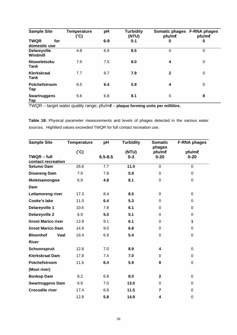
56

Sample Site Temperature pH Turbidity Somatic phages F-RNA phages (˚C) (NTU) pfu/mℓ pfu/mℓ TWQR for domestic use

6-9 0-1 0 0

Delareyville Windmill

4.8 6.9 8.5 0 0

Ntsweletsoku Tank

7.6 7.5 8.0 4 0

Klerkskraal Tank

7.7 6.7 7.9 2 0

Potchefstroom Tap

8.5 6.4 5.9 4 0

Swartruggens Tap

5.6 6.8 8.1 0 8

TWQR – target water quality range; pfu/mℓ – plaque forming units per millilitre.

Table 18: Physical parameter measurements and levels of phages detected in the various water

sources. Highlited values exceeded TWQR for full contact recreation use.

Sample Site Temperature pH Turbidity Somatic phages

F-RNA phages

(˚C) (NTU) pfu/mℓ pfu/mℓ TWQR – full contact recreation

6.5-8.5 0-3 0-20 0-20

Setumo Dam 26.6 7.7 11.0 0 0

Disaneng Dam 7.9 7.8 5.9 0 0

Moletsamongwe

Dam

6.9 4.8 8.1 0 0

Letlamoreng river 17.3 8.4 8.5 0 0

Cooke’s lake 11.0 6.4 5.3 0 0

Delareyville 1 10.6 7.8 6.1 0 0

Delareyville 2 6.9 5.0 5.1 0 0

Groot Marico river 12.8 9.1 6.1 0 1

Groot Marico Dam 14.9 9.0 6.8 0 0

Bloemhof Vaal

River

16.4 6.9 5.4 0 0

Schoonspruit 12.8 7.0 8.9 4 0

Klerkskraal Dam 17.8 7.4 7.0 0 0

Potchefstroom

(Mooi river)

11.6 6.4 5.9 8 0

Boskop Dam 8.2 6.8 8.0 2 0

Swartruggens Dam 6.9 7.0 13.0 0 0

Crocodile river 17.4 6.8 11.5 7 0

12.8 5.8 14.9 4 0

57

Sample Site Temperature pH Turbidity Somatic phages

F-RNA phages

(˚C) (NTU) pfu/mℓ pfu/mℓ TWQR – full contact recreation

6.5-8.5 0-3 0-20 0-20

Lendlyspoort Dam

Vaalkop Dam 13.9 6.6 12.0 2 0

TWQR – target water quality range; pfu/mℓ – plaque forming units per millilitre.

An expansion of the phage measurements in the Mooi river catchment is provided in Figure

18. Physico-chemical parameters from these sources were within TWQRs for various uses

including recreation and livestock watering (Table 19). Results indicated that very high levels

of phages are present in this river system, particularly in the borehole samples. The lower

phage levels presented in Table 17 and 19 could be due to slight methodology differences.

Table 19: Physical parameter measurements detected in the various water sources in the Mooi River

Catchments area in 2012.

Sample Site Temp (˚C) pH Conductivity (mS/m)

DO mg/mℓ

TWQR – Recreational use

6.0-9.0 0-70

Muiskraal 9.1 8.48 44.5 8.6

Around the world bridge

11.5 8.41 66.4 8.6

Potch dam 11.8 8.45 68.3 8.8

Viljoenskroon road bridge

73.7 8.47 10.0 8.0

Mooi river and Vaal river confluence

11.6 8.57 54.1 9.8

Borehole samples

Trimpark 19.9 7.58 94.3 2.3

School 22.4 7.16 126.1 3.5

Cemetery 22 7.10 33.4 2.2

Temp = temperature; TWQR = target water quality range; DO = Dissolved oxygen; mS/m = micro Siemens per

meter

More coliphages were detected in the borehole samples. Somatic coliphages averaging

4.3x104 pfu/mℓ and F-specific coliphages at 5.3X103 pfu/mℓ. Somatic coliphages from the

surface water averages at 4.1x102 pfu/mℓ and F-specific coliphages at 1.4x102 pfu/mℓ.

58

Figure 18: Comparison of coliphage counts isolated from surface water (Sites 1-5) and groundwater

(Trim Park, School & Cemetery) samples.

2.4 Conclusions

• Physico-chemical results for surface water indicated that the water was generally

suitable for several purposes such as full contact recreational as well as domestic

use. This was reflected by TWQRs (DWAF, 1996). Although electrical conductivity

(or TDS) for some of the sources was high, there were no cases of the levels being

such that they would cause negative health implications if the water is consumed

without treatment. This elevated EC could be indicative of increasing salinisation, one

of the problems identified by DWAF (2009) for the Vaal River. Elevated EC was also

observed at sites in the Harts River.

• Enterococcus sp. as well as Escherichia coli, were isolated from various surface

water sources. This demonstrates that surface water of the North West Province is

contaminated by various faecal indicator bacteria. Several of these are potentially

pathogenic species if the correct conditions prevail.

• It was also demonstrated that several of the yeast species were found in the surface

water sources of the North West Province. These included the following genera

Candida, Clavispora, Cryptococcus, Cystofilobasidium Hanseniaspora, Meyerozyma,

Pichia, Rhodotorula, Saccharomyces, Sporidiobolis, and Wickerhamomyces. Some

the species of these genera could cause invasive infections as opportunistic

pathogens if sensitive individuals are exposed to them.

1

10

100

1000

10000

Somatic coliphages

F-specific coliphage

59

• This study provides baseline data on the investigation of the dominant bacterial

communities in the Vaal River using molecular methods including DGGE and High

Throughput Sequencing. Although there are some limitations to DGGE analysis, this

approach permitted the identification of the bacterial community compositions which

may have not been detected with cultivation-based methods. Due to the limitations,

HTS analysis was applied in this study that presented a better resolution of the

bacterial diversity and dominant groups in the Vaal River. Data of the present study

may be useful in future bacterial community studies that might be investigating the

links between pollution and microbial community dynamics.

• Bacteriophages were detected in several potable and non-potable water sources.

The results of the non-potable water sources support the general findings of the

bacterial analysis i.e. that many of the water sources in the North West Province

have some form of faecal pollution. The major concern is that several of the potable

water sources were also contaminated as demonstrated by bacteriophage results. A

further worrying aspect is that some of the wastewater treatment plants were

decanting up to 106 enterovirus particles/mℓ into surface water sources. The qPCR

method could not determine the viability of the virus particles. However, such high

concentrations of enteroviruses flowing into surface water sources is of concern

particularly if one considers that bacterial and yeast opportunistic pathogens were

also detected in the surface water sources.

60

CHAPTER 3

GROUNDWATER QUALITY IN THE NORTH WEST PROVINCE

3.1 Introduction

Apart from the surface water resources, the NWP has a large reservoir of subterranean

water in the form of fractured aquifers and dolomitic compartments (Kalule-Sabiti & Heath,

2008). Dolomitic aquifers are porous, facilitating fast and easy infiltration into this

groundwater resource, therefore increasing the risk and probability of contamination.

Anthropogenic activities exert strong pressures on groundwater resources (Murray et al.,

2004; Usher et al., 2004b). A study by Kwenamore (2006) showed relatively high bacteria

counts of total and faecal coliforms in groundwater from the Disobotla and Molopo districts

of the Province. It is known that elevated faecal coliforms in water may pose a public

health risk (Bezuidenhout et al., 2002; Stevens et al., 2003).

In the NWP cultivated agriculture lands are either dryland or irrigation farming. In the latter

case surface and/or groundwater is used. In many cases livestock receives water from

groundwater sources (NWDACE, 2008). The rural communities of the NWP require about

70 million m3 water per annum. Of this 25 million m3 per annum is used for domestic

consumption and the remainder is used for livestock-watering and irrigation agriculture

(NWDACE, 2008). Studies demonstrated that solid waste dumps, grey water, animal

rearing activities and pit latrines are major non-point sources related to shallow

groundwater quality problems in informal settlements in South Africa, including the NWP

(Dzwairo et al., 2006; Kulabako et al., 2007).

In most instances, commercial farmers have boreholes that are drilled much deeper into the

underground aquifers that rural those of informal communities. The greater vertical distance

of deeper boreholes and the absence of open pit latrines, leads to these boreholes being

less-contaminated than shallow wells mostly found in informal settlements. The results of

Gallegos et al. (1999) support this deduction. The authors detected higher coliform counts in

shallow (<10 m) boreholes than deeper boreholes. Informal dwellers usually use these

shallow wells (Gallegos et al, 1999), that are in many cases not properly sealed and which

may be exposed to open faecal pollution for abstracting drinking water (Dzwairo et al., 2006;

Griesel et al., 2006; Kulabako et al., 2007; Grönwall et al. 2010).

Research by the CSIR showed that groundwater in the NWP has high concentrations of

fluoride and nitrate (Ashton, 2009). In many areas the concentrations of these substances

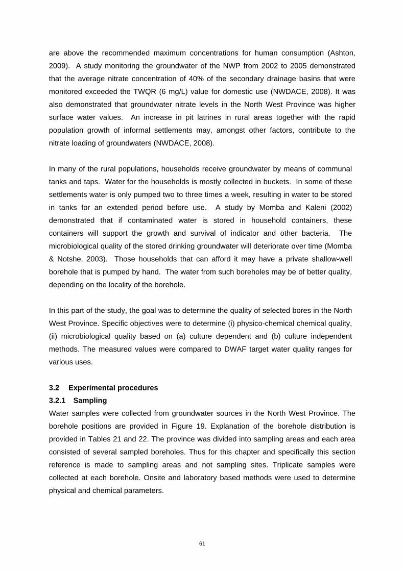
61

are above the recommended maximum concentrations for human consumption (Ashton,

2009). A study monitoring the groundwater of the NWP from 2002 to 2005 demonstrated

that the average nitrate concentration of 40% of the secondary drainage basins that were

monitored exceeded the TWQR (6 mg/L) value for domestic use (NWDACE, 2008). It was

also demonstrated that groundwater nitrate levels in the North West Province was higher

surface water values. An increase in pit latrines in rural areas together with the rapid

population growth of informal settlements may, amongst other factors, contribute to the

nitrate loading of groundwaters (NWDACE, 2008).

In many of the rural populations, households receive groundwater by means of communal

tanks and taps. Water for the households is mostly collected in buckets. In some of these

settlements water is only pumped two to three times a week, resulting in water to be stored

in tanks for an extended period before use. A study by Momba and Kaleni (2002)

demonstrated that if contaminated water is stored in household containers, these

containers will support the growth and survival of indicator and other bacteria. The

microbiological quality of the stored drinking groundwater will deteriorate over time (Momba

& Notshe, 2003). Those households that can afford it may have a private shallow-well

borehole that is pumped by hand. The water from such boreholes may be of better quality,

depending on the locality of the borehole.

In this part of the study, the goal was to determine the quality of selected bores in the North

West Province. Specific objectives were to determine (i) physico-chemical chemical quality,

(ii) microbiological quality based on (a) culture dependent and (b) culture independent

methods. The measured values were compared to DWAF target water quality ranges for

various uses.

3.2 Experimental procedures

3.2.1 Sampling

Water samples were collected from groundwater sources in the North West Province. The

borehole positions are provided in Figure 19. Explanation of the borehole distribution is

provided in Tables 21 and 22. The province was divided into sampling areas and each area

consisted of several sampled boreholes. Thus for this chapter and specifically this section

reference is made to sampling areas and not sampling sites. Triplicate samples were

collected at each borehole. Onsite and laboratory based methods were used to determine

physical and chemical parameters.

62

Fig

ure

19:

A m

ap in

dica

ting

the

loca

tions

of t

he b

oreh

oles

sam

pled

in 2

009

and

2010

.

63

Table 20: Sample areas (A09-J09) number and distribution of boreholes sampled in 2009.

Sample date Sample Areas

Season n – number of boreholes sampled in area 16/2/2009 Klerksdorp; Stilfontein; Orkney; Mooibank; Potchefstroom

A09 Summer n = 8 10/3/2009 Carletonville-Ventersdorp Fochville-Welverdiend

B09 Summer n = 5

26/3/2009 Lichtenburg; Koster; Doornkop; Makokskraal; Derby;

Coligny C09 Summer n = 7 4/4/2009 Hartbeespoortdam; Brits; Matrooster; Rustenburg

D09 Autumn n = 8

17/4/2009 Hartbeespoortdam

E09

Autumn n = 5 9/5/2009 Delareyville; Zeerust; Mafikeng; Stella; Setlagole; Ottosdal

F09 Autumn n = 8 26/5/2009 Schweizer-Reneke; Bloemhof; Wolmaransstad; Christiana

G09 Autumn n = 5 10/6/2009 Vryburg-Ganyesa

H09 Winter n = 4

23/6/2009 Bray; Vostershoop; Piet-Plessis; Makopeng;

Molopo;Tseoge I09 Winter n = 9

26/7/2009 Taung; Salpeterspan; Sekhing; Geluk; Amalia; Reivilo J09 Winter n = 9

Table 21: Sample areas (A10-J10) number and distribution of boreholes sampled in 2010.

Sample date Sample Areas Season n – quantity boreholes sampled in area

12/04/2010 Klerksdorp; Stilfontein; Orkney; Potchefstroom A10 Autumn n = 5

27/04/2010 Ventersdorp; Coligny; Lichtenburg; Biesiesvlei;

Sannieshof B10 + C10 Autumn n = 6

10/05/2010 Hartbeespoortdam; Brits; Derby; Rustenburg D10 Autumn n = 5

18/05/2010 Delareyville-Ottosdal; Zeerust; Mafikeng; Geysdorp;

Setlagole; F10 Autumn n = 5

23/03/2010 Schweizer-Reneke; Bloemhof; Wolmaransstad G10 Autumn n = 7

64

Sample date Sample Areas Season n – quantity boreholes sampled in area

31/05/2010 Vryburg; Ganyesa; Broedersput H10 Autumn n = 4

24/05/2010 Taung; Hartswater; Sekhing; Amalia; Christiana J10 Autumn n = 6

3.2.2 Physico-chemical parameters

Details are provided in section 2.2.2

3.2.3 Culturable indicator bacteria

Details are provided in section 2.2.3.

In addition, mannitol salt agar was used for enumeration of Staphylococcus aureus.

Incubation was at 37ºC for 24 hours. On these plates – small to large yellow colonies

surrounded by a yellow zone were counted.

Dilutions up to 10-6 were made for the enumeration of heterotrophic plate count bacteria, of

which 0.1 mℓ was used to make a spread plate on R2A agar. The incubation period was 5

days at room temperature. Results were expressed as colony forming units per mℓ.

Presumptive Pseudomonas aeruginosa were isolated from m-FC agar plates (grey colonies).

Representative grey colonies from each borehole (when present) were sub-cultured onto

nutrient agar plates. If the nutrient agar plates changed colour to green after a 24 hour at

37ºC incubation period it was noted as potentially P. aeruginosa. E. coli were identified by

biochemical methods including API 20 E (bioMerieux, Inc. Hazelwood) according to the

instruction of the manufacturer. Identities confirmed by PCR amplification of the lacZ and

mdh genes.

For the isolation of E. coli, the same methods were followed as described in section 2.2.3.

However, in 2010 a different selective agar was used to enumerate total coliforms and

E. coli. Membrane lactose glucuronide agar (MLGA) (Oxoid, UK) was used to enumerate

E. coli (green colonies) and total coliforms (green and yellow colonies). This agar

substituted M-Endo agar for the enumeration of total coliforms, while also providing valuable

E. coli counts. MLGA plates were incubated for 24 h at 37°C. The remainder of the

selective agars for bacterial enumeration was the same as those used in 2009.

65

3.2.4 Detection and identification of E. coli directly from water samples

Multiplex PCR (mPCR) was used to detect the presence of E. coli without culturing in

borehole water samples. DNA was isolated directly from borehole water samples using the

NexttecTM Genomic DNA isolation kit for bacteria (NexttecTM Biotechnology GmbH,

Germany). See section 2.2.5 for more details of the DNA isolation process. The mPCR was

optimised to simultaneously amplify fragments two of the E. coli house-keeping genes

[malate dehydrogenase gene (mdh) and of the lactose promoter (lacZ)]. Each reaction

consisted of 1 x PCR Mastermix (2 mM MgCl2, 0.2 mM of each dNTP, 0.025 U/μl Taq-

polymerase; Fermentas Life Sciences, US) forward and reverse primers (1μM; Table 22),

additional (0.5 mM) MgCl2 and (0.1 mM) betaine. RNase/DNase free PCR grade water

(Fermentas Life Sciences, US) was used to make a final volume of 25 μl. One hundred

nanogram of DNA was used as template in each reaction. Cycle conditions consisted of:

initial denaturation at 95°C for 300 seconds, 40 cycles of denaturation at 95°C for 30

seconds, annealing at 55°C for 30 seconds and extension at 72°C for 60 seconds. Final

extension was at 72ºC for 300 seconds. PCR reactions were processed in an ICycler (Bio-

Rad, UK). Agarose electrophoresis was used to visualise the PCR fragments.

Table 22: Primer sets used in the E. coli multiplex PCR.

Primer Specificity Sequence (5’ 3’) Size

(bp) Reference

mdh E. coli FW: GGTATGGATCGTTCCGACCT

RV: GGCAGAATGGTAACACCAGAGT 301 Tarr et al., 2004.

lacZ E. coli FW: CTGGCGTAATAGCGAAGAGG

RV: GGATTGACCGTAATGGGATATG 228 Ram & Shanker, 2005

3.2.5 Bacterial diversity by High Through-put sequencing

Water from two of the boreholes were selected and analysed by HTS as described in section

2.2.5. One sample was from a rural borehole that is used for agricultural purposes (near

Schweizer-Reineke). The other sample was from a rural town (Wolmaransstad) and in this

case was used for drinking purposes. In each case a sample was collected in summer and

one in winter.

66

3.2.6 Statistical analysis

See section 2.2.7

3.3 Results and Discussion

3.3.1 Physico-chemical quality

The sampling sites were grouped into sample areas (A to J). In 2009 a total of 76 boreholes

were sampled and in 2010, 38. pH levels for groundwater were within the TWQR for

domestic use (pH 6-9). What is of concern is the very high electrical conductivity and nitrates

(Tables 24 and 25). The nitrate levels are further explored in Figures 20 and 21.

Table 23: Physico-chemical data of water from boreholes for various sampling areas (A09 – J09)

measured in 2009. The details of the area location are found in Table 17. Highlighted values

exceeded TWQR for domestic use.

Sample pH Temp EC Nitrate – nitrogen Area

TWQR

6-9

(°C)

(mS/m)

0-70 mS/m

(mg/ℓ NO3-N)

0-6 mg/ℓ Min 6.8 20.4 34.7 1.8

A09 Max 7.6 24.5 140.0 209.8 Ave±SD 7.1±0.3 22.9±1.4 88.4±41.03 33.1±71.4

Min 6.8 21.1 6.7 0.1 B09 Max 7.9 22.3 70.0 3.0

Ave±SD 7.4±0.4 21.6±0.5 44.7±23.7 0.9±1.2 Min 6.9 20.6 12.7 4.5

C09 Max 7.5 26.0 135.0 120.9 Ave±SD 7.1±0.2 23.0±6.9 66.2±41.8 58.7±59.2

Min 7.1 20.2 48.9 0.9 D09 Max 8.1 24.1 122.5 55.2

Ave±SD 7.3±0.4 23.0±1.8 90.0±26.5 14.1±6.9 Min 6.4 19.2 31.2 0.3

E09 Max 7.7 24.3 114.6 8.4 Ave±SD 7±0.4 22.4±1.6 81.9±30.1 5.9±3.3

Min 6.8 21.0 21.4 0.6 F09 Max 7.6 22.4 121.8 160.0

Ave±SD 7.2±0.3 21.6±0.9 90.2±32.7 12.4±11.5 Min 6.9 18.6 57.4 5.5

G09 Max 7.5 19.5 175.8 47.0 Ave±SD 7.1±0.4 18.7±2.1 97.6±48.9 32.2±14.9

Min 6.7 16.6 96.0 38.6 H09 Max 7.0 18.5 173.1 63.6

Ave±SD 6.9±0.1 17.7±0.8 124.7±33.6 49.9±10.7 Min 7.1 16.2 63.7 0.5

I09 Max 8.2 24.0 113.4 454.5 Ave±SD 7.4±04 20.6±2.6 91.2±16.3 171.6±188.2

Min 7.0 15.5 75.8 3.9 J09 Max 8.8 21.5 144.5 454.5

Ave±SD 7.4±0.5 19.7±2.1 106.2±24.5 210.7±223.1

67

Min 6.4 15.5 6.7 0.1 Total 76 Max 8.8 24.5 175.8 454.5 Boreholes Ave±SD 7.2±0.4 20.9±3.2 89.1±35.8. 67.0±124.3

Min – minimum; Max – maximum; SD – standard deviation Ave – average; Temp – temperature; EC – electrical conductivity; TDS – total dissolved solids

Table 24: Physico-chemical data of water from boreholes for various sampling areas (A10 – J10)

measured in 2010. The details of the area location are found in Table 18. Highlighted values

exceeded TWQR for domestic use.

Sample pH Temp EC Nitrate – nitrogen

Area

TWQR

6-9

(°C)

(mS/m)

0-70 mS/m

(mg/ℓ )

0-6 mg/ℓ

Min 6.9 20.9 64.1 0.8 A10 Max 8.7 22 146.4 11.4

Ave 7.4±0.7 21.7±0.5 103.0±36.3 8.3±4.4 Min 6.8 19.5 22.3 11.1

B + C10 Max 7.3 21.1 183.1 74.1 Ave 7.2±0.2 20.3±0.7 72.7±58.5 30.1±25.8 Min 6.7 18.8 11.3 0.7

D10 Max 7.6 23.5 95.2 44.3 Ave 7.1±0.3 21.2±2.2 59.3±35.3 12.6±18.0 Min 7.0 18.1 62.4 8.2

F10 Max 7.8 20.5 253.0 23.9 Ave 7.4±0.4 20.3±0.9 134.2±74.4 15±6.5 Min 6.7 20.8 66.9 23.3

G10 Max 7.2 25.8 90.5 148.2 Ave 7.0±0.4 23.9±2.0 77.1±15.1 44±42.0 Min 7.1 16.0 80.4 15.2

H10 Max 7.6 21.2 125.9 28.9 Ave 7.4±0.2 18. 6±2.4 103.9±25.1 23.3±6.7 Min 6.8 19.4 86.1 1.6

J10 Max 7.7 24.4 286.0 23.2 Ave 7.3±0.4 22.0±2.0 149.0±72.3 13.5±8.7 Min 6.7 16.0 11.3 0.7

Total 38 Max 8.7 25.8 286.0 74.1 Boreholes Ave 7.2±0.4 21.1±2.1 98.2±56.3 24.9±27.4

Min – minimum; Max – maximum; SD – standard deviation Ave – average; Temp – temperature; EC – electrical conductivity; TDS – total dissolved solids.

68

Figure 20: A log graph of the nitrate levels of the boreholes sampled in 2009. The x-axis represents

the individual boreholes (1 to 76) and the horizontal line represents that 20 mg/ℓ level above which

methaemoglobinemia is most likely to occur if young children and infants were to consume the water.

Each bar in Figures 19 and 20 represents the nitrate concentrations (logarithmic scale) of

each borehole sampled individually. Figure 19 indicates the levels of nitrates measured in

2009. In some cases nitrate levels were alarmingly high. The average nitrate levels of only

two sampling areas (B09 and E09) were within the TWQR for domestic use (<6 mg/ℓ NO3-N).

In six of the ten sampling areas average nitrate levels exceeded 20 mg/ℓ NO3-N. A total of

thirty-one (40.8%) of the boreholes sampled in 2009 had nitrate concentrations exceeding

this limit. Methaemoglobinemia in infants and young children may occur if this high nitrate

load is consumed over an extended period of time (Sadeq et al., 2008). Furthermore, in six

of the sampling areas, average nitrate concentration exceeded the maximum acceptable

value of nitrate for the use of irrigation purposes (30 mg/ℓ NO3-N; DWAF, 1996). The

average nitrate level for all 76 boreholes sampled was a very high (67.0 mg/ℓ NO3-N). In

areas I09 and J09 the highest nitrate levels (171.6±188.2 and 210.7±223.1, respectively)

were measured.

69

Figure 21: A log graph of the nitrate levels of the boreholes sampled in 2010. The x-axis represents

the individual boreholes (1 to 38) and the horizontal line represents that 20 mg/ℓ level above which

methaemogloninemia is most likely to occur if young children and infants were to consume the water.

In 2010 the observed nitrate levels were, in many cases, higher than the 6 mg/ℓ NO3-N

TWQR for domestic use (Figure 21). However, the levels were lower than those measured

in 2009. The average nitrate level for all the boreholes sampled in 2010 were 24.9±27.4

mg/ℓ NO3-N compared to the 67.0±124.3 mg/ℓ NO3-N of 2009 (Table 22). None of the areas

sampled in 2010 had average nitrate levels below 6 mg/ℓ NO3-N. The highest measured

nitrate level was from a borehole in area G10 (148.2 mg/ℓ NO3-N). Areas I09 and J09 both had

boreholes with nitrate levels at 450.0 mg/ℓ NO3-N or higher. The average nitrate level of

sample area J, situated in the western part of the province, was much higher in 2009 than

in 2010. The average for area J10 was 13.5±8.7 mg/ℓ and that for J09 210.7±223.1 mg/ℓ

NO3-N. Although the boreholes sampled during these two periods were in the same

sampling areas, they were not exactly the same ones. This finding, however, indicates that

some boreholes within sample areas had water of different qualities that could potentially

be ascribed different aquifers. Boreholes from B09 had the lowest average nitrate levels

(0.9±1.2 mg/ℓ NO3-N) in 2009 but the second highest average nitrate levels (30±25.8 mg/ℓ

NO3-N) in 2010. Sixteen (42.1%) of the boreholes sampled in 2010 exceeded the critical

methaemoglobinemia causing limit (20 mg/ℓ NO3-N; x-axis) whereas 40.8% of the

boreholes sampled in 2009 exceeded this limit (Table 25).

70

Table 25: Summary of percentage boreholes that exceeded TWQR values as well as those

exceeding levels that are most likely to cause methaemoglobinemia.

2009 2010

% Boreholes exceeding domestic TWQR (6 mg/ℓ) 67.0 82.0

% Boreholes exceeding definite methaemoglobinemia

causing levels (20 mg/ℓ) 40.8 42.1

3.3.2 Bacteriological quality of borehole water

Table 24 summarises the minimum, maximum and average heterotrophic plate count

bacteria (HPC), total coliforms, faecal coliforms and enterococci counts of each of the 10

sample areas of 2009. Samples were also screened for the presence of the opportunistic

pathogens Pseudomonas aeruginosa and Staphylococcus aureus. Results for the latter two

were reported as the percentage of boreholes from each sample area that tested positive for

the opportunistic pathogens.

Faecal coliforms were detected in at least one borehole water sample from every sample

area. Three sample areas (A09, B09, and D09) had at least one borehole with enterococci

counts exceeding 300 cfu/100 mℓ (Table 24). Based on the average counts of all the

indicator bacteria (Table 24), it is demonstrated that area B09 was highly contaminated by

faecal and other bacteria. This area (B09) is located in the south-eastern part of the North

West Province and includes Ventersdorp, Carletonville and Fochville. These are urban areas

but recently there had been sanitation and water quality issues in some of the towns

(http://www.pmg.org.za/print/29951). Area J09 had the lowest overall bacterial counts. This

area (J09) is located in the south-western part of the Province and the boreholes are

generally deep. Area A09 to E09 was sampled in the warm and wet season and F09 to J09 was

sampled in the cold and dry winter season. Average faecal coliform and enterococci counts

were lower in area E09 to J09 with the exception of area I09 which had a high average faecal

coliform (70±95.6 cfu/100 mℓ) as well as enterococci (56±52.0 cfu/100 mℓ) count. This

observation could statistically be linked to lower ambient and water temperature (Figure 25).

Pseudomonas aeruginosa was detected in 46% of the 76 boreholes sampled and

Staphylococcus aureus in 7% (Table 26). Staph. aureus were detected in only four of the 10

sample areas. A future study on occurrence and distribution of Staph. aureus in groundwater

in the province could focus on the areas that were positive and determine the potential

source of the pollution.

71

Table 26: Indicator bacteria counts and % of boreholes that were positive for S. aureus and P.

aeruginosa of areas A-J sampled in 2009.

HPC – Heterotrophic plate count; TC – Total coliforms; FC – Faecal coliforms; FS – Enterococci; Min – minimum

count; Max – maximum count; Ave – Average count; SD –Standard deviation; cfu – colony forming unit.

Thirty eight boreholes were sampled during the 2010 sampling period. Table 25 shows the

microbiological results of each sample area for this period. Compared to 2009

microbiological results the 2010 results included E. coli and excluded the opportunistic

pathogen S. aureus. Membrane Lactose Glucuronide agar (MLGA) was used as substitute

for m-Endo agar that was used in 2009. MLGA selects for and differentiate between E. coli

and total coliforms. In 2009 several false positives were observed with the use of Mannitol

Salt agar (MSA) for the detection of S. aureus. Also, a minority of the sites sampled in 2009

Sampling Area HPC TC FC FS P. aeruginosa S. aureus

cfu/mℓ cfu/100 mℓ cfu/100 mℓ cfu/100 mℓ %Present %PresentTWQR - Domestic 0-100 0-5 0 N/A

A09 Min 34 12 0 0

0% 13% Max 3076 >300 200 >300 Ave±SD 798±1089.2 >76±92.7 34±68.7 >49±104.0

B09 Min 60 17 8 2

0% 0% Max 3100 >300 260 >300 Ave±SD 1145±1240.9 >182±108.0 140±97.7 >125±160.3

C09 Min 87 16 0 0

0% 22% Max 4666 180 163 50 Ave±SD 1490±1437.7 60±54.8 36±57.3 7±16.5

D09 Min 180 23 0 0

75% 14% Max 3360 215 106 >300 Ave±SD 1468±1226.9 92±63.8 38±46.1 >87±145.8

E09 Min 47 7 0 0

100% 0% Max 1333 230 92 9 Ave±SD 451±560.9 62±77.0 12±32.5 2±3.2

F09 Min 43 2 0 0

75% 0% Max 7500 220 104 5 Ave±SD 2205±2645.7 54±69.4 14±36.3 1±1.7

G09 Min 10 0 0 0

100% 13% Max 1900 230 20 54 Ave±SD 933±722.7 52±76.4 4±7.1 12±21.9

H09 Min 133 6 0 5

0% 0% Max 3000 77 42 7 Ave±SD 2117±2661.8 31±32.2 11±21.0 6±1.0

I09 Min 166 30 0 1

75% 0% Max 1263 >300 280 159 Ave±SD 660±340.9 >114±94.5 70±95.6 56±52.0

J09 Min 50 5 0 0

44% 0% Max 400 120 3 94 Ave±SD 228±122.7 47±39.2 <1±1.0 12±30.8

Overall Min 10 0 0 0 Max 7500 >300 280 >300 46% 7% Ave±SD 1068±1400.6 >75±78.6 33±62.9 >33±77.2

72

were positive for S. aureus. Therefore, enumeration of this opportunistic pathogen was

excluded from the 2010 sampling period.

Table 27: Indicator organism’s counts and % boreholes that were positive for P. aueruginosa of areas

A-J sampled in 2010.

HPC – Heterotrophic plate count; TC – Total coliforms; FC – Faecal coliforms; FS – Enterococci; Min – minimum

count; Max – maximum count; Ave – Average count; SD – Standard deviation; cfu – colony forming unit.

A large proportion of the boreholes sampled in 2010 had faecal coliforms present. Of

particular concern was that some of the boreholes from areas F10 and J10 had faecal

coliforms levels exceeding 300 cfu/100 mℓ (Table 27). The boreholes from J09 (Table 26)

had the least number of faecal coliforms present during the 2009 sampling period. This

discrepancy was due to the inclusion of the Hartswater samples in the 2010 sampling period.

Water samples from boreholes from this area had very high levels of faecal coliforms and

other bacteria.

Enterococci levels in borehole water samples were lower 2010 compared to the 2009

samples. The average 2010 enterococci counts for all the boreholes sampled were 10±29.2

Area HPC TC FC E. coil

FS P. aeruginosa

cfu/mℓ cfu/100 mℓ cfu/100 mℓ cfu/100 mℓ cfu/100 %Present TWQR - Domestic 0-100 0-5 0 0 N/A

A10 Min 110 0 0 0 2

40% Max 800 21 17 1 8 Ave±SD 341±290.6 8.2±10.8 5±7.3 <1±0.4 2±3.5

B+C10 Min 163 0 0 0 0

50% Max 1 393 98 15 12 10 Ave±SD 547±490.5 34±39.2 6±6.3 4±4.0 5±3.5

D10 Min 273 0 0 0 0

0% Max 4 066 280 126 36 26 Ave±SD 1833±1769.9 58±124.1 26±56.0 7±16.0 5±11.5

F10 Min 20 3 0 0 0

60% Max 5 500 >300 >300 34 8 Ave±SD 2129±2241.7 >62±133.3 >68±130.2 8±14.8 4±3.8

G10 Min 70 0 0 0 0

100% Max 647 5 2 2 8 Ave±SD 208±190.6 1±2.1 <1±0.8 <1±0.8 3±3.4

H10 Min 0 0 0 0 0

25% Max 966 300 220 0 6 Ave±SD 425±495.4 75±150 55±110 0 2±2.8

J10 Min 100 2 0 0 10

83% Max 3 650 >300 >300 3 180 Ave±SD 943±1340.1 >96±134.0 >64±118.1 <1±1.4 45±66.9

Overall

Min 0 0 0 0 0 55% Max 5 500 >300 >300 36 180

Ave±SD 898±1293.3 >46±95.6 >29±76.6 3±8.0 10±29.2

73

cfu/100 mℓ compared to the 2009 average of >33±77.2 cfu/100 mℓ. Area J10 had the highest

average for enterococci (45±66.9 cfu/100 mℓ). This could once again be ascribed to the

Hartswater samples. The remainder of the 2010 sample areas (A10 – H10) had low

enterococci averages.

A higher percentage of boreholes had P. aeruginosa present in 2010 (55%) compared to

2009 (46%). Only one of the sample areas of 2010 (D10), tested negative for P. aeruginosa

and four (A09, B09, C09 & H09) in 2009. P. aeruginosa was detected in all of the boreholes

sampled in area G10.

Over the two sampling periods, a total of 114 boreholes were sampled. Of these boreholes,

88% tested positive for total coliforms, 50% for thermo-tolerant faecal coliforms and 68% for

enterococci. These results indicate that several groundwater sources in the NWP are

contaminated by faecal matter that could be of human or non-human origin. The results of

this study are reflective of the results of Kwenamore (2006). That study sampled 304

groundwater sources from the Ditsobotla and Molopo districts in the NWP. Samples were

taken twice seasonally; winter and spring in 2003 and summer and autumn in 2004. Faecal

and total coliform bacteria, Enterococcus spp., Klebsiella spp. and Citrobacter spp. were

detected throughout the sampling period (Kwenamore, 2006).

Indicator bacteria in the groundwater may promote additional deterioration of the water

quality during its residence time in storage tanks and household containers. Studies by

Momba and Kaleni (2002) and Momba and Notshe, (2003) showed that these containers will

support the growth and survival of indicator bacteria and that the microbiological quality of

the stored drinking groundwater will deteriorate consistently with the length of storage.

Groundwater as a source for domestic use is almost always stored in large storage tanks.

Inhabitants of informal settlements in rural areas usually store their water in smaller

household containers (e.g. 20ℓ). The drinking water containers of communities in the North

West Province may thus harbour various indicator and other bacterial species. This is an

aspect that could be further explored in future studies.

With the groundwater study the focus was on determining the identity of faecal coliforms

using API 20 E. Of the 110 selected faecal coliform isolates tested with the API 20 E system,

98 were identified at 90% or greater accuracy. Amongst these 98 representatives the

following enteric bacteria from the family Enterobacteriaceae was confirmed. Enterobacter

cloacae (34%), Enterobacter aerogenes (31%), Klebsiella pneumonia (15%), Escherichia

coli (10%), Raoutella planticola (4%), Raoutella terrigena (3%), and Pantoea spp. 2 (3%).

74

E. coli identified were isolated from the following boreholes and sample areas: Stilfontein

(A09); Fochville, Ventersdorp 1 and Ventersdorp 2 (B09); Groenfontein (C09); Matrooster (D09);

Stella (F09); Christiana 1 (G09); and Tseoge and Molopo (I09).

Thirty-two of the 38 boreholes sampled in 2010 were screened for the presence of E. coli

using mPCR. Area H was sampled in the beginning 2010 when the DNA isolation directly

from water and mPCR conditions had not been optimised. Therefore, this area was

excluded. The remaining 32 borehole samples were clustered into three groups. This

grouping was done based on their culture based microbiological results. The mPCR was

performed on each of the three groups. All the samples that had presumptive E. coli present

(green colonies on MLGA) were grouped (Figure 22). Faecal coliform positive sites (blue

colonies on m-FC agar) that had no green colonies on MLGA were grouped (Figure 23).

The third group consisted of three sites that were positive for total coliforms (yellow colonies

on MLGA) but negative for faecal coliforms and E. coli (lane 1-3; Figure 24), and nine sites

that were negative for total coliforms, faecal coliforms and E. coli (lane 4-12; Figure 24).

75

Figure 22: A 1.5% (w/v) Ethidium bromide stained agarose gel illustrating multiplex PCR results for

boreholes that tested positive for E. coli on MLGA. One hundred nanograms of DNA were used as

template. The left lane contains a 100bp molecular marker (O’GeneRulerTM 100bp DNA ladder,

Fermentas Life Sciences, US). Lane 1 – Wolmaransstad; lane 2 – Potchefstroom2; lane 3 –

Potchefstroom-Ventersdorp; lane 4 – Biesiesvlei; lane 5 – Sannieshof; lane 6 – Coligny-Biesiesvlei;

lane 7 – Brits; lane 8 – Rustenburg2; lane 9 – Zeerust; lane 10 – Delarey-Ottosdal; lane 11 –

Setlagole; lane 12 – Sekhing; and Lane 13 – Christiana. The last two lanes contain the positive

(+cont. E. coli ATCC 10536) and no template controls (-cont.).

Figure 23: A 1.5% (w/v) ethidium bromide stained agarose gel illustrating multiplex PCR results for

boreholes that tested positive for faecal coliforms on m-Fc agar but negative for E. coli on MLGA.

One hundred nanograms of DNA were used as template. The left lane contains a 100bp molecular

marker (O’GeneRulerTM 100bp DNA ladder, Fermentas Life Sciences, US). Lane 1 – Klerksdorp; lane

2 – Potchefstroom1; lane 3 – Geystown; lane 4 – Taung; lane 5 – Hartswater; lane 6 – Christiana2;

and lane 7 – Ganyea. The last two lanes contain the positive (+cont. E. coli ATCC 10536) and no

template controls (-cont.).

76

Figure 24: A 1.5% (w/v) ethidium bromide stained agarose gel illustrating multiplex PCR results for

boreholes that tested positive for total coliforms on MLGA but negative for E. coli on MLGA and faecal

coliforms on m-Fc (lane 1-3). Lane 4-12 represents multiplex PCR results for boreholes that tested

negative for total coliforms, faecal coliforms and E. Coli. One hundred nanograms of DNA were used

as template. The left lane contains a 100bp molecular marker (O’GeneRulerTM 100bp DNA ladder,

Fermentas Life Sciences, US). Lane 1 – Ventersdorp-Coligny; lane 2 – Mafikeng; lane 3 – Amalia;

lane 4 – Orkney; lane 5 – Stilfontein; lane 6 – Lichtenburg; lane 7 – Derby; lane 8 – Hartbeespoort;

lane 9 – Rustenburg; lane 10 – Broedersput; lane 11 – Vryburg; and lane 12 – Ganyesa2. The last

two lanes contain the positive (+cont. E. coli ATCC 10536) and no template controls (-cont.).

Two distinct bands of PCR product of the expected fragment size for the mdh and lacZ

primer sets were visible in lanes 1, 3, 4, 5, 7, 8 and 9 of Figure 22. Faint bands were visible

in lanes 6, 11, 12 and 13. Lane 2 and 10 were negative for the target E. coli gene

fragments. The culture based method therefore gave two potentially false positives for

E. coli (lane 2 and 10). Potchefstroom2 (lane 2) had one green colony (presumptive E. coli)

on MLGA in a 100 ml of sample water and Delarey-Ottosdal (lane 10) had two. Overall

results indicate that the selective and differential agar, MLGA, was 85% accurate in the

positive detection E. coli, given that all the sites represented by lane 1-13 tested positive for

E. coli when MLG-agar was used. Due to the low number of E. coli detected in a 100 ml of

sample by MLGA for Potchefstroom 2 and Delarey-Ottosdal, it is possible that E. coli could

have been detected by PCR if extraction were preceded with a 1-3 hour enrichment period.

Boreholes sampled in both the sampling periods (2009 and 2010) were situated on farms as

well as rural settlements. Almost all the boreholes from rural settlements were shallow wells

pumped by hand. The remainder of the boreholes sampled were situated on small-holdings

and towns. It was expected that the main source of faecal contamination would be from

animal origin. Farm animals (cows, chickens, pigs and horses) were found grazing in close

proximity to most of the boreholes. In the case of the shallow wells found in the rural

77

settlements, faecal contamination from human and animal origin was expected. Most of the

shallow wells sampled in rural settlements were situated in close proximity to open pit

latrines. Water abstracted from a shallow well within a lateral distance of about 25 m from a

pit latrine may be contaminated by faecal bacteria (Dzwairo et al., 2006). In most cases

these shallow wells are not maintained or sealed properly at the ground surface, increasing

the potential for contamination (Gallegos et al., 1999).

The ratio between faecal coliform and enterococci was used to indicate the most likely

source of faecal contamination. A study by Jagals et al. (1995) supports the assumption that

the origin of faecal contamination is more likely to be animal waste if enterococci counts are

higher than that of faecal coliforms. The movement of animal wastes (frequently applied as

soil fertilisers) into groundwater is often cited as a major factor contributing to the pollution of

groundwater (Cho et al., 2000). Even though there were mixed indications of the origin of

faecal pollution, it was established that water sources were polluted and that the species

isolated could have health implications for humans.

The faecal coliforms (FC) and faecal streptococci (FS) ratio can be used as an indication of

the possible source of contamination (Csuros& Csuros, 1999; Wyer & Kay, 1995). Table 28

summarises the % boreholes from each sample area that had a 1) FC/FS ratio <0.7,

indicating possible contamination from non-human origin; 2) FC/FS ratios between 2 and 4,

indicating possible contamination from human waste; 3) FC/FS ratios >4, indicating possible

human faecal matter contamination (Csuros& Csuros, 1999; Wyer & Kay, 1995) and 4) the

% boreholes that were negative for faecal coliforms as well as faecal streptococci.

78

Table 28: FC/FS ratios of 2009 and 2010.

2009 Sampling period

% FC/FS ratio % boreholes no FC or

FS detected

2010 Sampling period

% FC/FS ratio % boreholes no FC or

FS detected <0.7 2-4

>4 <0.7 2-4

>4

A09 50 13 13 13 A10 0 40 0 40 B09 20 20 40 0 B+C10 33 33 0 17 C09 33 0 44 22 - - - - - D09 57 0 29 14 D10 0 20 20 60 E09 38 0 13 50 - - - - - F09 25 13 25 38 F10 20 0 20 20 G09 38 13 13 38 G10 43 0 0 57 H09 75 0 25 0 H10 50 0 25 25 I09 55 11 11 0 - - - - - J09 55 0 0 33 J10 50 17 0 0 Total 76 boreholes 45 7

20 22

Total 38 boreholes 32 16

8 32

In Table 28 it is demonstrated that non-human origin (FC/FS ratio <0.7) of faecal

contamination was more common in both sampling compared to contamination by human

waste (FC/FS ratio 2-4) or human faecal matter (FC/FS ratio >4). This may be so because

the majority of boreholes sampled were situated on farms and rural areas. Areas B09, C09

had a high percentage of boreholes with possible contamination from human sources. This

was not the case for area B+C10. None of the boreholes from sample areas B09, H09, I09 and

J10 tested negative for both faecal coliforms and faecal streprococci, indicating that

boreholes from these areas were all subjected to faecal contamination. All the boreholes of

the latter sample areas (B09, H09, I09 and J10), except for area B09, were indicated to be mainly

contaminated from non-human faecal sources. It was also observed that the samples from

area C09 were predominantly contaminated by human faecal waste. The overall 20% of

boreholes in 2009 and 8% in 2010 that had FC/FS ratio >4 is cause for concern and needs

to be further investigated.

Canonical ordination redundancy analysis (RDA) was applied to determine the correlation

between the environmental variables (temperature, TDS, EC and NO3-N) and the indicator

bacteria levels detected in 2009 and 2010. Mean biplots were used to visualise the results

of the multi-variate analysis. The biplots represent the joint effect of environmental variables

on the selected bacteria in a single plane (Ter Braak, 1990). The angles in the biplot

between the response (indicator bacteria) and environmental variables, and between the

response variables themselves or environmental variables themselves, reflect their

79

correlations. Figure 25 shows the RDA biplot obtained from using the environmental

variable data and bacterial counts of 2009 and Figure 26 provides the latter for the 2010

data.

Figure 25: Correlation biplot of the relationship between the environmental variables and indicator

bacteria levels measured during the 2009 sample period. Environmental variables are represented by

red arrows and include: water temperature (Temp), pH, total dissolved solids (TDS) and electrical

conductivity (EC). Indicator bacteria are represented by blue arrows and include: faecal streptococci

(FS), faecal coliforms (FC), total coliforms (TC) and heterotrophic plate count bacteria (HPC).

The biplot (Figure 25) shows that the two environmental variables having the closest

correlation with faecal coliforms (FC) and faecal streptococci (FS) were temperature (Temp)

and pH. Furthermore, a strong correlation also existed between FC and FS. Total coliforms

(TC) and heterotrophic plate count (HPC) bacteria were strongly correlated. Total coliform

counts were more strongly correlated with pH than HPC bacteria. On the other hand HPC

bacterial levels were strongly correlated with EC than TC. Nitrate-nitrogen (NO3-N) levels

did not show a correlation to levels of any of the bacterial tested for. Biplots of the 2010

results are shown in Figure 26.

80

Figure 26: Correlation biplot of the relationship between the environmental variables and indicator

bacteria levels measured during the 2010 sample period. Environmental variables are represented by

red arrows and include: water temperature (Temp), pH, total dissolved solids (TDS) and electrical

conductivity (EC). Indicator bacteria are represented by blue arrows and include: E. coli, faecal

streptococci (FS), faecal coliforms (FC), total coliforms (TC), and heterotrophic plate count bacteria

(HPC).

The biplot (Figure 26) shows that the environmental variable having the closest correlation

with faecal coliforms (FC), faecal streptococci (FS) and total coliforms (TC) were electrical

conductivity (EC). Nitrate-nitrogen levels showed a weak correlation with E. coli.

Furthermore, a strong correlation between heterotrophic plate count (HPC) bacteria and E.

coli is also observed. This was also seen for TC and FC. In the 2010 analysis none of the

bacteria showed a correlation with temperature.

3.3.3 Bacterial diversity by High Through-put sequencing

The relative abundance of various bacterial phylogenetic groups in the water of the

boreholes are depicted in Figures 27 and 28. In both cases the uncultured bacterial

component was greater (70.55-78.09%) in the winter when compared to the summer

samples (31.65 to 34.79%). In the summer samples of both the boreholes the Gamma and

Beta proteobacteria as well as Actinobacteria made up greater proportions of the bacterial

community structure. Among the Gamma proteobacteria, Enterobacter sp., Proteus sp.,

Stenotrophomonas maltophilia are species that were always detected. There were also

several other species that were consistent with the culture dependent results. Sequences

from E. coli as well as Pseudomonas sp. and Staph aureus were also detected in the

summer samples.

81

The most important message from these results is that HTS is a powerful tool to provide

data on the microbial diversity in borehole water. Results are generated much quicker and

presence of indicator bacteria were also demonstrated.

Figure 27: The relative abundance and composition of the dominant bacterial phylogenetic groups in

the groundwater obtained through high-throughput sequencing for the Wolmaransstad borehole.

82

Figure 28: The relative abundance and composition of the dominant bacterial phylogenetic groups in

the groundwater obtained through high-throughput sequencing for the Schweizer-Reneke borehole.

3.4 Conclusion

• All water samples complied with the domestic use TWQR for pH (DWAF, 1996).

Although EC readings were mostly high, the values were also at acceptable levels for

domestic use. Nitrate contamination was the major contaminant. Twenty eight

percent of all the boreholes tested complied with the national nitrate limit (6 mg/L

NO3N) for drinking water. Forty three percent of the boreholes had nitrate levels

greater than 20 mg/L NO3-N. Some of the levels were greater than 400 mg/L NO3-N.

• Microbiological results showed that groundwater of the North West Province may be

prone to contamination from faecal sources. The study also showed that

opportunistic pathogens (P. auruginosa and Staph aureus) associated with faecal

pollution are present in the water from some boreholes.

83

• Next generation sequencing (or high through-put sequencing) results provided data

on the microbial diversity in borehole water. This method is fast in comparison to

culture based methods. It was demonstrated that this method holds promise to be

used in monitoring indicator bacterial species in groundwater.

84

CHAPTER 4

QUANTIFICATION OF FAECAL STEROLS IN ENVIRONMENTAL WATERS

4.1 Introduction

Sewage tracers can be used to examine a) the presence of current, past, sewage inputs and

b) the distribution and transport of sewage in the environment (Pratt, 2005). In this respect,

the biomarkers are organic compounds that, once released into the environment, retain their

structural integrity for their source to be recognised (Leeming et al., 1996). The distribution of

sterols found in faeces and hence their source-specificity, depends on the animal’s ability to

synthesise its own sterols as well as the intestinal micro-biota (Leeming, 2006).

Combinations of these factors determine “the sterol fingerprint”. Field studies (Leeming,

1996) and a major validation study (Leeming et al., 1998) highlighted the possibility of using

sterols in combination with bacterial indicator concentrations as faecal pollution indicators in

any water column.

The principal human faecal sterol, coprostanol (COP; 5β(H)-cholestan-3β-ol) constitutes

about 60% of the total sterols found in human faeces. Coprostanol itself is not a contaminant

of concern, but it provides the opportunity to assess other particulate bound contaminants

such as viruses, PCB’s, bacteria, hydrocarbons and endocrine disrupters (Writer et al.,

1995). Coprostanol is much more stable and resistant to environmental changes compared

to faecal coliform bacteria (Nishimura and Koyama, 1977). The C29 homologue of

coprostanol is 24-ethylcoprostanol (24-ethyl-5β(H)-cholestan-3β-ol) which is the main faecal

sterol excreted by herbivores. Both coprostanol and 24-ethylcoprostanol are present in

different ratios in both human and animal faeces. It is possible to determine the relative

contributions by calculating the ratio of coprostanol to 24-ethylcoprostanol in human and

herbivore (e.g. sheep, cow, and possum) faeces (Leeming et al., 1996). Cholesterol (CHL;

5-cholesten-3β-ol) is the main sterol synthesised in the body of animals, and is absent from

prokaryotes (bacteria) and plants. It is not completely absorbed by the body and is also

excreted as a component of bile (Anon2, 2007).

Stigmasterol (SROL; 3β-hydroxy-24-ethyl-5,22-cholestadiene) is an un-saturated plant sterol

occurring in plant fats and oils (Baxter et al., 1999), whereas stigmastanol (SNOL; β-

sitostanol) is an algae sterol and is found in reducing environments. Stigmastanol’s presence

in water indicates algae presence and does not signify human or animal waste (Pratt et al.,

2007). β-sitosterol (β-SIT; 24β-ethylcholesterol) is a phytosterol. It originates from a wheat

85

germ, peanuts, soybeans, pumpkin seeds and corn oil. The presence β-sitosterol in water

thus indicates sterols originating from plants and not humans or animals (Lam, 2009).

The naturally occurring stanol in unspoiled environments is 5α-cholestanol (DCHL;

dehydrocholesterol). It is thermodynamically the most stable isomer. By comparing ratios of

coprostanol to 5α-cholestanol (Leeming and Nichols, 1995), one can determine if

coprostanol found in organic–rich, or anaerobic sediments are of faecal origin.

Dehydrocholesterol is found in trace amounts (relative to coprostanol) in human faeces, but

increases in relative proportions in digested sewage sludges (Leeming, 2006). Increased

amounts of dehydrocholesterol relative to coprostanol indicate older human faecal

contamination (such as faecal sludges from sewer pipes). Measurement of these sterols

from a non-faecal origin in the water column indicates that organic matter had been re-

suspended from highly anaerobic sediments (Leeming, 2006).

Sterols are extracted and isolated from surface water samples and wastewater samples by

liquid-liquid extraction using dichloromethane. Coprostanol, however, has an a-polar

character, which slightly reduces its solubility in dichloromethane, making it more difficult to

recover. A surrogate solution is added (perylene) in order to test the recovery of the sterols

in the water samples. An internal standard (perylene-d12) is added to quantitate the sterols

that elute (Szűcs et al., 2006). Because significant differences occur in individual

composition of human and animal faeces due to alterations in dietary intake, sterol patterns

in water can provide information to distinguish, and determine the origin of faecal pollution.

High ratios of coprostanol could be associated with anthropogenic faecal contamination in

water, while abundances in cholesterol and β-sitosterol are typical sterols from dogs or birds

(Szűcs et al., 2006). In accordance, herbivore profiles have terrestrial sterols and

phytosterol abundances.

Faecal sterols in biological and environmental samples are usually quantitated by using gas

chromatographic (GC) techniques such as, GC with flame ionisation detection (FID) (Batta et

al., 2002) and GC-electron capture detection (Jayasinghe et al., 1998). Identification is

confirmed by GC-MS (mass spectrometry) (Batta et al., 2002). Because cost and

effectiveness is of concern when testing environmental water samples for faecal sterol

content, the identification and quantitation of sterols in a single chromatographic run is of

importance. The objectives of this study was to use the validated Szűcs method (Szűcs et

al., 2006) in determining faecal sterol fingerprints for various animal species and humans, as

well as the quantitation of these sterol profiles and the differences between each of the

86

profiles. This method was also evaluated for the presence of faecal sterols in selected

surface and groundwater sources.

4.2 Experimental procedures

The method used was from Szűcs et al. (2006), with some modifications. This (Szűcs et al.,

2006) was used to validate simultaneous determination of faecal sterols in water by gas

chromatography-mass spectrometry. Only six target sterols (COP, CHL, DCHL, SROL,

SNOL, β-SITO) were analysed in this method.

Dichloromethane (HPLC grade), acetonitrile (HPLC grade), sodium hydroxide, and

standards of faecal sterols (COP, CHL, DHCL, SROL, SNOL, β-SIT) as well as the

surrogate standard solution (Perylene), and the internal standard (Perylene-d12) were all

provided by Sigma-Aldrich (Stenheim, Germany). N,O-bis-trimethylsilyl-trifluoroacetamide

(BSTFA) with 1% trimethylchlorosilane (TMCS) was from Supelco (Germany).

4.2.1 Preparation of standard solutions

For optimisation of GC-MS conditions, a standard mixture of COP, CHL, DCHL, SROL, β-

SIT, SNOL, and perylene (surrogate standard) was prepared in dichloromethane at a

concentration of 1.0 mg/mℓ for each component. For quantitative determination, perylene-

d12 was used as an internal standard (IS) and dissolved in dichloromethane to obtain a

stock solution of 1.0 mg/mℓ. In order to determine the extraction efficiency (recovery) of the

faecal sterols in unknown water samples, a 0.25 mg/mℓ perylene surrogate standard solution

was prepared in acetonitrile.

4.2.2 Derivatisation procedure

The GC-MS analysis of target sterols was carried out after derivatisation with BSTFA-TMCS.

A 25 μℓ aliquot of the standard mixture as well as 20 μℓ of IS solution was pipetted into 1.5

mℓ auto sampler vial (Supelco, Germany) and dried completely under nitrogen flow. The

residue was reconstituted in 125 μℓ of dichloromethane and mixed with 125 μℓ of BTSFA-

TMCS. The vial was closed with a Teflon-lined screw cap, and the sample was silylated at

70˚C for 30 min. Following derivatisation, 1 μℓ of the mixture was injected into the GC-MS.

4.2.3 Instrumentation and GC-MS conditions

The samples were analysed on a Hewlett-Packard (Palo Alto, CA) GC-MS system consisting

of an HP 6890 GC with an HP 5973 mass selective detector (MSD) and an Agilent 7683

automatic liquid sampler (Agilent Technologies, Palo Alto, CA). Separations were

accomplished using an Supelco Equity-5 fused silica capillary column (Hewlett-Packard)

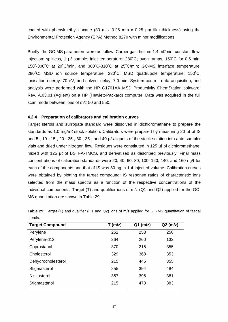
87

coated with phenylmethylsiloxane (30 m x 0.25 mm x 0.25 μm film thickness) using the

Environmental Protection Agency (EPA) Method 8270 with minor modifications.

Briefly, the GC-MS parameters were as follow: Carrier gas: helium 1.4 mℓ/min, constant flow;

injection: splitless, 1 μℓ sample; inlet temperature: 280˚C; oven ramps, 150˚C for 0.5 min,

150˚-300˚C at 20˚C/min, and 300˚C-310˚C at 25˚C/min; GC-MS interface temperature:

280˚C; MSD ion source temperature: 230˚C; MSD quadrupole temperature: 150˚C;

ionisation energy: 70 eV; and solvent delay: 7.0 min. System control, data acquisition, and

analysis were performed with the HP G1701AA MSD Productivity ChemStation software,

Rev. A.03.01 (Agilent) on a HP (Hewlett-Packard) computer. Data was acquired in the full

scan mode between ions of m/z 50 and 550.

4.2.4 Preparation of calibrators and calibration curves

Target sterols and surrogate standard were dissolved in dichloromethane to prepare the

standards as 1.0 mg/mℓ stock solution. Calibrators were prepared by measuring 20 μℓ of IS

and 5-, 10-, 15-, 20-, 25-, 30-, 35-, and 40 μℓ aliquots of the stock solution into auto sampler

vials and dried under nitrogen flow. Residues were constituted in 125 μℓ of dichloromethane,

mixed with 125 μℓ of BSTFA-TMCS, and derivatised as described previously. Final mass

concentrations of calibration standards were 20, 40, 60, 80, 100, 120, 140, and 160 ng/ℓ for

each of the components and that of IS was 80 ng in 1μℓ injected volume. Calibration curves

were obtained by plotting the target compound: IS response ratios of characteristic ions

selected from the mass spectra as a function of the respective concentrations of the

individual components. Target (T) and qualifier ions of m/z (Q1 and Q2) applied for the GC-

MS quantitation are shown in Table 29.

Table 29: Target (T) and qualifier (Q1 and Q2) ions of m/z applied for GC-MS quantitation of faecal

sterols.

Target Compound T (m/z) Q1 (m/z) Q2 (m/z)

Perylene 252 253 250

Perylene-d12 264 260 132

Coprostanol 370 215 355

Cholesterol 329 368 353

Dehydrocholesterol 215 445 355

Stigmasterol 255 394 484

ß-sitosterol 357 396 381

Stigmastanol 215 473 383

88

Identity of the target sterols was examined by comparing the obtained mass spectra with

those of the corresponding reference substances using the HP 5973 MSD reference

collection, NIST MS search program, and spectrald database collection, Version 1.5 (1996)

(Hewlett-Packard).

4.2.5 Preparation of water samples for GC-MS analysis

A raw domestic wastewater sample (influent) was obtained from an urban sewage treatment

plant (Potchefstroom Wastewater Treatment Plant) as well as a treated wastewater sample

(effluent). Surface water samples were also spiked with faeces from animals (cattle,

chickens, horses, pigs and sheep). Samples were processed for extraction within 24-36 h.

Water samples (300 mℓ) were mixed with 200 μℓ of 0.125 mg/mℓ surrogate standard solution

and 10 g NaOH. Samples were then saponified in a shaking incubator at 60˚C for 1 h.

Following saponification, the spiked water samples and the effluent were extracted (see

section on recovery), derivatised (see section on derivatisation procedure), and analysed by

GC-MS (see section on instrumentation and GC-MS conditions). The untreated wastewater

sample (influent) was prepared for GC-MS in the same manner, but it was mixed with 50 mℓ

of dichloromethane and ultra-sonicated with 10μm amplitude for 10 min before extraction.

Concentrations of target sterols and surrogate were calculated on the basis of calibration

curves by the data analysis software (HP ChemStation)

Groundwater samples (300 ml) were collected from boreholes and surface water samples

from several sites in the North West Province and analysed by using the Szucs et al. (2006)

method.

4.3 Results and Discussion

Standard curves (Figure 29) were constructed by dividing the area of the peak for perylene-

d12 (IS), by the area of the peak for each of the target sterols (COP, CHL, DCHL, SROL,

SNOL, β-SIT). This was done for each concentration of the standard solution. The ratios

were determined and plotted on a concentration/response graph.

The calibration curves for COP, CHL, DCHL, SROL, β-SITO and SNOL were obtained from

three different series. Target compound-IS response ratios were linear up to 160ng for each

target sterol molecule. Lines of best fit obtained by linear regression were described by:

COP: y = 0.0311x – 0.1999, where r2 = 0.9094; CHL: y = 0.0311x – 0.2285, where r2 =

0.9044; DCHL: y = 0.0499x – 0.2802, where r2 = 0.9339; SROL: y = 0.0353x – 0.2711,

where r2 = 0.8995; Β-SITO: y = 0.0268x – 0.2131, where r2 = 0.8981;

SNOL: y = 0.0504x – 0.3302, where r2 = 0.9250.

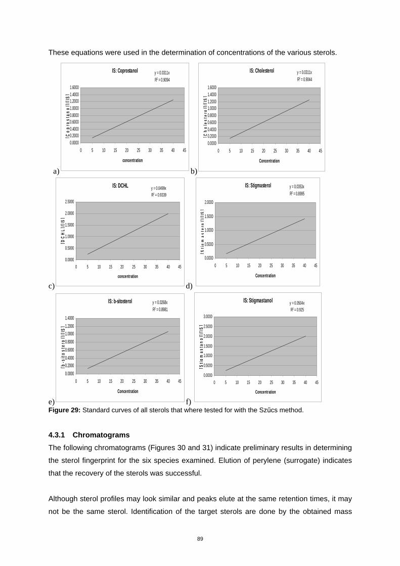
89

These equations were used in the determination of concentrations of the various sterols.

a) b)

c) d)

e) f) Figure 29: Standard curves of all sterols that where tested for with the Szűcs method.

4.3.1 Chromatograms

The following chromatograms (Figures 30 and 31) indicate preliminary results in determining

the sterol fingerprint for the six species examined. Elution of perylene (surrogate) indicates

that the recovery of the sterols was successful.

Although sterol profiles may look similar and peaks elute at the same retention times, it may

not be the same sterol. Identification of the target sterols are done by the obtained mass

IS: Coprostanol y = 0.0311xR2 = 0.9094

0.00000.20000.40000.60000.80001.00001.20001.40001.6000

0 5 10 15 20 25 30 35 40 45

concentration

[Co

pro

stan

ol]

/[IS

]IS: Cholesterol y = 0.0311x

R2 = 0.9044

0.00000.20000.40000.60000.80001.00001.20001.40001.6000

0 5 10 15 20 25 30 35 40 45

Concentration

[Ch

ole

ster

ol]

/[IS

]

IS: DCHL y = 0.0499xR2 = 0.9339

0.0000

0.5000

1.0000

1.5000

2.0000

2.5000

0 5 10 15 20 25 30 35 40 45

concentration

[DC

HL

]/[I

S]

IS: Stigmasterol y = 0.0353xR2 = 0.8995

0.0000

0.5000

1.0000

1.5000

2.0000

0 5 10 15 20 25 30 35 40 45

Concentration

[Sti

gm

aste

rol]

/[IS

]

IS: b-sitosterol y = 0.0268xR2 = 0.8981

0.0000

0.2000

0.4000

0.6000

0.8000

1.0000

1.2000

1.4000

0 5 10 15 20 25 30 35 40 45

Concentration

[b-s

ito

ster

ol]

/[IS

]

IS: Stigmastanol y = 0.0504xR2 = 0.925

0.0000

0.5000

1.0000

1.5000

2.0000

2.5000

3.0000

0 5 10 15 20 25 30 35 40 45

Concentration

[Sti

gm

asta

no

l]/[

IS]

spectra

some c

by the M

Establis

sterol a

(Leemin

sterols

a)

b)

a for each e

compound m

MS detecto

shing stero

analysis and

ng et al., 1

and one su

eluted comp

may overlap

r, were use

l fingerprin

d helps wit

996). GC-M

rrogate. Pe

pound and

p during elu

d to identify

ts is neces

h understa

MS conditio

eaks of all th

90

not by rete

ution. Targe

y target ster

ssary becau

nding the o

ons were o

he target ste

ention time

et and qual

rols of all sp

use it form

origin of fae

optimised w

erols could

s. This is n

ifier ions (T

pecies.

s the base

ecal pollutio

with a stand

be seen (Fi

necessary b

Table 28), o

eline for the

on in a wat

dard mixtur

igures 30 a

because

obtained

e faecal

ter body

re of six

nd 31).

c)

d)

Figure 3

Figure 3

to level

such re

Table 2

Elution

abunda

levels t

eluted d

30: The stero

30a shows

ls of copros

esults indica

2.

of choleste

ances. Thos

that their qu

dehydrocho

ol profiles of

higher abu

stanol. This

ate faecal p

erol and th

se of cattle

uantities co

olesterol and

the herbivor

ndance of c

s is in agre

pollution fro

e phytoster

(Figure 30

ould not be

d stigmaste

91

re species; a

cholesterol

eement with

om birds. Th

rol, β-sitost

0b) and hor

e determine

erol that was

a.) chicken, b

and β-sitos

h Szűcs et

his phenom

terol, occur

rse (Figure

ed. Horse s

s not found

b.) cattle, c.)

sterol was o

al., (2006)

menon is als

rs in all ste

30c) profile

terol profile

in the stero

horse and d

observed co

), which su

so demonst

erol profiles

e were of s

e (Figure 3

ol profile of

.) sheep.

ompared

ggested

trated in

s, at low

such low

0c) also

the cow

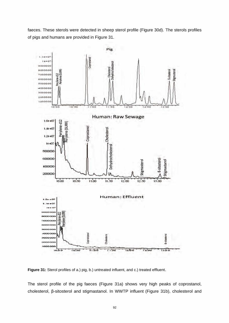
faeces.

of pigs

Figure 3

The ste

choleste

These ster

and human

31: Sterol pro

erol profile

erol, β-sitos

rols were de

ns are provid

ofiles of a.) p

of the pig

sterol and

etected in s

ded in Figu

pig, b.) untrea

faeces (Fi

stigmastano

92

sheep stero

re 31.

ated influent

igure 31a)

ol. In WWT

ol profile (Fig

t, and c.) trea

shows ver

TP influent

gure 30d). T

ated effluent.

ry high pea

(Figure 31b

The sterols

.

aks of copr

b), choleste

s profiles

rostanol,

erol and

93

coprostanol was found. Coprostanol is the main human faecal sterol biomarker, indicating

fresh human faecal contamination (Leeming, 1996; Szűcs et al., 2006). All other five sterols

were found in varying concentrations. Coprostanol, cholesterol and β-sitosterol was found in

very low levels in WWTP effluent (Figure 31c).

Comparing the sterol profiles of pigs (Figure 31a) and sewage (Figure 31b), a distinct

difference between the two profiles can be seen. All target sterols eluted in the sewage

sterol profile (Figure 31b). Levels of β-sitosterol and the terrestrial sterols (stigmastanol and

stigmasterol) were all low. Coprostanol and cholesterol were present at higher concentration.

The pig sterol profile (Figure 31a) had high coprostanol but low cholesterol levels. The

concentration of dehydrocholesterol and stigmastanol were much higher in the pig profile

than in the WWTP influent profile (Figure 31b).

Comparing the WWTP influent sterol profile (Figure 31b) to the treated effluent (Figure 31c),

it can be deducted that the target sterols tested for in this study has been radically

decreased or completely removed. There were also fewer peaks in the treated water

demonstrating that the wastewater treatment works was removing sterols from wastewater.

This result implies that one could evaluate the efficiency of wastewater treatment plants

using GC-MS analysis of faecal sterols.

In all the samples that contained mainly human faecal matter, the concentration of

coprostanol and cholesterol concentrations were higher than the other sterols. In the case of

cow, horse, sheep and chicken faecal samples, the concentration of coprostanol was lower

than other sterols. This observation forms the basis for differentiating human from non-

human sources of faecal contamination in environmental water samples.

Concentrations of the various sterols that eluted are important because from the

concentrations, ratios can be established (Leeming, 2006). The ratios of the concentrations

are used to determine the origin of faecal pollution. Concentrations of the target sterols were

calculated by integrating the peaks that eluted for each species and determining the area of

each peak. Using the standard curve’s y-values and r2-values, the concentrations of each

sterol that eluted for each of the various species could be calculated by the straight line

equation: y = mx + c. The values are depicted in Table 30.

94

Table 30: Concentrations of all marker sterols that eluted for the seven samples analysed.

COP CHL DCHL SROL ß-SITO SNOL

(ppm) (ppm) (ppm) (ppm) (ppm) (ppm)

Chicken 29.998 81.126 0 0 119.828 0

Cow 0 5.859 0 0 4.875 0

Horse 0 3.785 4.740 3.078 8.024 0

Sheep 26.995 12.698 21.227 8.442 28.126 74.828

Pig 111.008 49.280 34.957 0 14.070 68.336

Sewage

Influent 14.297 15.012 1.685 0.636 3.513 1.012

Sewage

Effluent 1.368 2.004 0 0 2.887 0

Table 30 indicates that the treated effluent had very low concentrations of sterol to be of any

consequence. All species had cholesterol and β-sitosterol in their profiles. Sheep, horse, pig

and raw sewage samples had dehydrocholesterol and are consistent with observations by

Leeming, (2006). The WWTP influent, horse and sheep faecal samples were the only

profiles that had stigmasterols present. Large amounts of β-sitosterol were found among

horse and sheep profiles, but less in cow faeces. This is contradictory since these species

are all herbivores. All the herbivore species had large amounts of stigmastanol and

stigmasterol compared to the other species. This is because of their diet, as stigmasterol

and stigmastanol are both terrestrial sterol biomarkers (Leeming, 2006).

4.3.2 Surface and groundwater

Water samples collected from boreholes were subjected to analysis for faecal sterols. The

same groundwater samples were also analysed for physico-chemical properties and

bacteriological quality (Ferreira, 2011). Tables 32 and 33 are summaries of the results. The

electrical conductivity and nitrate levels were high, mostly exceeding the drinking water

TWQR (DWAF, 1996). These are discussed in Chapter 3 and implications further explored in

Chapter 5.

95

Table 31: Physico-chemical properties of the groundwater samples taken at the various sites.

Site pH Temp

(°C)

EC

(mS/m)

NO3-N

(mg/ℓ)

Mafikeng 7.1 19.3 141.6 8.2

Zeerust 7.8 20.1 62.4 9.5

Delarey-Ottosdal 7.2 20.5 133.2 23.9

Setlagole 7.0 19.5 253.0 18.4

Geystown 7.8 18.1 810.0 15.2

Taung 7.7 24.4 916.0 16.4

Hartswater 7.6 20.2 286.0 22.3

Sekhing 7.3 24.0 142.7 1.6

Christiana 7.5 19.4 143.7 23.2

Christiana 2 6.9 22.2 86.1 11.6

Vryburg 7.2 16.0 125.4 28.9

Ganyessa 7.5 17.3 125.9 28.6

Ganyessa 2 7.1 21.2 84.0 15.2

mS/m = micro Siemens per metre; mg/ℓ= milligram per litre; NO3-N=Nitrate-nitrogen

The values of the bacteriological counts are provided in Table 29. Very high total coliform

and faecal coliforms were detected in four of the boreholes samples. In the case of the

Hartswater sample the faecal streptococci levels were also high. These samples were also

analysed for the presence of faecal sterols. Most of the samples tested negative.

Chromatograms for the samples that were positive are shown in Figures 31 to 33.

Table 32: Bacterial counts for groundwater samples.

Site TC

(cfu/100 ml)

FC

(cfu/100 ml)

E. coli (cfu/100 ml)

FS

(cfu/100 ml)

Mafikeng 3 0 0 8

Zeerust 5 3 2 3

Delarey-Ottosdal 27 3 2 2

Setlagole >300 >300 34 8

Geystown 4 2 0 0

Taung 10 7 0 9

Hartswater >300 >300 0 180

Sekhing 5 3 2 10

Christiana 233 65 3 32

Christiana 2 26 9 0 18

96

Site TC

(cfu/100 ml)

FC

(cfu/100 ml)

E. coli (cfu/100 ml)

FS

(cfu/100 ml)

Vryburg 0 0 0 2

Ganyessa >300 220 0 6

Ganyessa 2 0 0 0 0

Figure 32: The GC-MS Chromatogram of the Christiana groundwater sample that was analysed for

faecal sterols.

The chromatogram (Figure 32) showed peaks for coprosanol and cholesterol in the

groundwater sample from Christiana. Coprostanol may indicate human and cholesterol

human or animal faecal pollution. These faecal sterols were also present in the GC-MS

chromatograms of Geystown and Taung samples (Figure 33). Both these samples had very

low levels of total coliforms (Table 31). They also did not have any E. coli present. Since

sterols interact with and become particle bound it was not expected to find any of these

organic substances in the groundwater. These positive results should be further explored in

future studies.

7.50 8.00 8.50 9.00 9.50 10.00 10.50 11.00 11.50 12.00 12.50 13.00

500000

1000000

1500000

2000000

2500000

3000000

3500000

4000000

4500000

5000000

5500000

6000000

Time-->

Abundance

TIC: CHRIST.D

7.50 8.00 8.50 9.00 9.50 10.00 10.50 11.00 11.50 12.00 12.50 13.00

500000

1000000

1500000

2000000

Time-->

Coprosanol

Cholestero

97

Figure 33: The GC-MS chromatograms of the (a) Geystown and (b) Taung groundwater samples that

were analysed for faecal sterols.

Surface water samples were also collected and analysed for the presence of faecal sterols.

These surface water samples were collected from the Baberspan Bird Sanctuary, previously

described. They were also analysed for their physico-chemical properties and levels of

bacteria (Molale, 2012). From Table 33 it is evident that the electrical conductivity for these

sites was high and that the nitrate levels were very low.

7.50 8.00 8.50 9.00 9.50 10.00 10.50 11.00 11.50 12.00 12.50 13.00

1000000

2000000

3000000

4000000

5000000

6000000

Time-->

Abundance

TIC: GEYSTWN.D

7.50 8.00 8.50 9.00 9.50 10.00 10.50 11.00 11.50 12.00 12.50 13.00

1000000

Time-->

Cholesterol

Coprostanol

7.50 8.00 8.50 9.00 9.50 10.0010.5011.0011.5012.0012.5013.00

500000

1000000

1500000

2000000

2500000

3000000

3500000

4000000

4500000

5000000

5500000

Time-->

Abundance

TIC: TAUNG.D

Pe

ry

len

e(

Su

rr

Pe

ry

len

e-

d1

2

7.50 8.00 8.50 9.00 9.50 10.0010.5011.0011.5012.0012.5013.00

500000

Time-->

ne

(S

ur

r

Coprostanol

Cholesterol

98

Table 33: Physico-chemical properties of the Baberspan samples.

Baberspan

sampling

pH Temp

(°C)

EC

(mS/m)

NO3-N

(mg/ℓ)

Harts river 8.6 12.0 147.1 1.2

Inflow 9.2 14.7 135.1 0.5

Hotel 8.6 15.2 115.2 0

Outflow 8.6 13.7 120.9 0.7

Table 34: Bacterial counts for the Baberspan water samples.

Baberspan

sampling

TC

(cfu/100ml)

FC

(cfu/100ml)

E. coli (cfu/100ml)

FS

(cfu/100ml)

Cholesterol

(ppm)

Harts river 265 130 3 127 0

Inflow 27 7 3 18 6.212

Hotel 19 1 1 50 6.008

Outflow 4 0 0 61 7.258

Bacterial counts for the Baberspan water samples were low, except for the Harts River site

(Table 34). All sites were positive for faecal streptococci. Low levels of faecal coliforms and

E. coli were detected at the inflow and the hotel sites. Water samples collected at the

Baberspan Bird Sanctuary were also analysed for faecal sterols using the Szucs method

(Szucs et. al., 2006). The only faecal sterol that was detected was cholesterol at the inflow,

hotel and outflow sites. No faecal sterols were detected at the Harts river site.

4.4 Conclusions

• Using water samples that were spiked with agricultural animal faeces as well as two

samples (influent and effluent) from a water treatment plant. faecal sterol profiles that

were animal species specific were generated. This demonstrated the potential of

using such an approach in source tracking faecal pollution in river systems in the

NWP.

• The potential of using this method for surface and groundwater studies to track

pollution was also demonstrated.

• Another potential application of the faecal sterol analysis is to use it to evaluate the

efficiency of wastewater treatment plants since it is a relatively quick method and

small amounts of water is needed to be analysed. This could prove to be very

beneficial since South Africa is a country of coherent wastewater treatment plant

failures (DWAF, 2009).

99

CHAPTER 5

WATER-RELATED HEALTH RISK POTENTIAL

5.1 Introduction

There is a close relationship between poverty and poor water quality available for domestic

use (Schreiner et al., 2002). In many cases poor communities are deprived of the benefits of

good quality water because they lack the finances as well as technological assets to

determine the quality of the water available of drinking purposes and, if necessary, initiate

remediation processes. They are thus forced to drink water, particularly surface water, of

low quality (Schreiner et al., 2002). In South Africa, in the recent past, several service

delivery social upheavals occurred due to the inability of local authorities to provide sufficient

quantity and acceptable quality of drinking water to these communities (e.g. Gaoganediwe,

2006; GCIS, 2005; Landman, 2009; Tempelhoff, 2009). Such urban South African

communities in these modern times are still deprived of sufficient water that is safe for

human consumption. This includes several communities in the North West Province and

these community members may be reliant on untreated water sources.

Health risks associated with untreated drinking water cause diseases such as shigellosis,

cholera, salmonellosis, diarrhoea and a variety of fungal, parasitic, bacterial and viral

infections (Zamxaka et al., 2004). A list of enteric diseases is presented in Table 1. The

majority infections from consuming untreated polluted water are associated with secondary

infections that are due to weakened defence mechanisms. People who are particularly

susceptible include very young children with underdeveloped immune systems, individuals

with compromised immune systems and the elderly with weakened immune systems (WHO

& UN-WATER, 2010). Patients under medical treatment after an organ transplant or

immune-compromising infections, such as AIDS (Acquired Immune Deficiency Syndrome),

are also at risk of infection (Pavlov et al., 2004). It is recognised that microbial flora of

humans play an important role in immunity to microorganisms (Candela et al., 2010).

However, individuals that are immune-compromised may not have such microbial flora. Such

immune-compromised individuals may even be infected by microorganisms that generally

have very low virulence and that would not typically infect healthy individuals (Glasmacher et

al., 2003). Studies on water quality and the impacts thereof should thus also determine the

general diversity of organisms present in the water samples. For this culture dependent as

well as culture independent methods are available. Both of these methods have advantages

100

as well as disadvantages when used in a study where the aim is to investigate potential

health impacts.

E. coli is used when the microbiological quality of water is determined (DWAF, 1996; Kong et

al., 2002; Lleo et al., 2005; Oliver et al., 2005). Although it is a commensal bacterium of

various animals inhabiting the colon, certain strains are pathogenic and infect mucosal

surfaces of the intestines (Kaper and Nataro 1998). Five groups of pathogenic E. coli are

known may use environmental water as a reservoir and transport agent after faecal

contamination (Kong et al. 2001; Ashbolt, 2004). These groups of E. coli are: (i) Entero-

Pathogenic E. coli (EPEC), (ii) Entero-Toxigenic E. coli (ETEC), (iii) Entero-Hemorrhagic

E. coli (EHEC), (iv) Entero-Invasive E. coli (EIEC) and (v) Entero-Aggregative E. coli (EAEC)

(Kaper, 2005; Nataro and Kaper, 1998). Under certain conditions chlorine treatment induces

E. coli into a viable but non-cultureable (VBNC) state (Oliver et al., 2005). This also holds

true for certain environmental conditions. The VBNC E. coli will not be detected by culture

based methods but will be able to cause infection (Lleo et al., 2005, Kong et al., 2002).

Polymerase chain reaction methods are available for the detection of E. coli. Multiplex PCR

methods had been developed for the identification of pathogenic E. coli from environmental

water sources (Omar et al., 2010; Bai et al., 2010; Wang et al., 2010; Rodas et al., 2009).

This is based on the direct PCR detection of several DNA markers by a single PCR (Omar et

al., 2010).

Besides bacteria, environmental water can also contain viruses and bacteriophages.

Municipal wastewater treatment systems, even in developed countries are capable of

reducing the load of these but in many cases cannot completely remove them from the

effluent (Carducci et al., 2008). This is particularly of concern if the poor state of waste water

treatment plants in South Africa is considered, particularly those decanting into the Vaal

River and its tributaries (DWA, 2009). In many cases these systems are exceeding their

design flow capacity, are not maintained, etc. (DWAF, 2012). These problems lead to poorly

treated (or untreated) sewage reaching the receiving waters. Within this matrix there will be

viruses that could have human health implications.

Yeasts of various types have been reported to have been isolated from lakes and ponds

(Sláviková & Vadkertiová, 1997; Medeiros et al., 2008), estuaries, coasts and mangrove

areas (van Uden & Fell, 1968) as well as oceans and the deep sea (Nagahama et al., 2003).

Only a few studies have reported on the presence of yeasts in river water (Sláviková &

Vadkertiová, 1997; Medeiros et al., 2008; van Wyk et al., 2012). Furthermore, more than

100 yeast species that are known to occur in environmental water sources have been

101

identified as human pathogens (Fromtling et al., 2003). A large percentage of these

pathogens are classified in the genus Candida. Hurley et al. (1987) list following pathogenic

yeasts that may be causal agents for candidosis: C. albicans, C. tropicalis, C. stellatoidea, C.

glabrata, C. krusei, C. parapsilosis, C. guilliermondii, C. viswanathii, Clavispora lusitaniae

(Candida lusitaniae) and Rhodotorula mucilaginosa (Rh.rubra).

There are major health risks associated with untreated drinking water because it may cause

diseases such as shigellosis, cholera, salmonellosis, diarrhoea and a variety of fungal,

parasitic, bacterial and viral infections (Zamxaka et al., 2004). Infectious particles and

pathogenic (potential pathogenic) microorganisms may cause various impacts on mucosal

cells of the intestine. Some of the impacts may be cytotoxic. In order for consumed microbes

to cause gastrointestinal diseases they must meet a number of virulence characteristics:

secrete extracellular enzymes, be cytotoxic to cells, adhere to cells, and survive passing

through the gastric fluids (Yuk, & Marshall, 2004). Various methodologies are available to

investigate cytotoxic effects. Each of these has their own advantages and disadvantages

(Lyle and Dufour, 1991).

This chapter is a focus on potential health implication of water samples collected during this

study and is based on potential use (general domestic and recreational). The objectives

were to:

1) use the microbial and physico-chemical quality data to determine if there are any health

risks associated if this water is used for domestic and recreational purposes;

2) determine antibiotic resistance and haemolytic potential of selected isolates and comment

on the potential human health risks;

3) investigate if pathogenic strains of E. coli are present in selected environmental water

sources;

4) determine the general microbial diversity in surface and groundwater sources by using

culture independent methods and whether amongst these there may be potential pathogens.

5) comment on the detection of enteroviruses in treated sewage and sewage-contaminated

water sources in selected water sources in the North West Province, South Africa;

6) develop and test a MTT method to determine the cytotoxicity effects on intestinal cells.

102

5.2 Experimental procedures

5.2.1 Physico-chemical parameters

Details of investigation are provided in Chapters 2, 3 and 4

5.2.2 Culturable bacteriological parameters

Details of investigation are provided in Chapters 2 and 3

5.2.3 Antibiotic resistance and haemolytic patterns

Antibiotic susceptibility tests were performed on faecal coliforms and enterococci isolates

using the Kirby-Bauer disk diffusion method (Bauer et al., 1966). Overnight cultures of faecal

coliforms and enterococci were grown in Brain Heart Infusion Broth (BHI) (Merck, Germany)

at 37°C and spread onto Mueller Hinton agar (Merck, Germany). In addition to the antibiotics

listed in Table 35, Neomycin (30 µg) Penicillin G (10 µg) and Vancomycin (30 µg) were used

for enterococci. For this group (enterococci) Cephalothin and Kanamycin was not included.

All antibiotics were obtained from Mast Diagnostics (UK). After incubation inhibition zones

were measured in millimetres and compared to the NCCLS growth inhibition zone standards

for Streptococci (NCCLS. 1999).

Table 35: Details of the antibiotics used in this study. The susceptibility specifications are only for E.

coli (NCCLS, 1999).

Antibiotic Classification

Antibiotics Abb Conc (µg)

Resistant (mm)

Intermediate Resistant

(mm)

Susceptible (mm)

Penicillin Β-lactam& derivatives

Ampicillin AMP 10 ≤ 13 14-16 ≥ 17

Cephalothin CEP 30 ≤ 14 15-17 ≥ 18

Amoxicillin AMOX 20 ≤ 13 14-17 ≥ 18

Amino-glycosides

Kanamysin Streptomycin

KAN STR

30 10

≤ 13 ≤ 11

14-17 12-14

≥ 18 ≥ 15

Quinolones Ciprofloxacin CIP 5 ≤ 15 16-20 ≥ 21

Trimethoprim Trimethoprim TM 1.25 ≤ 10 11-15 ≥ 16

Chloram-phenicol

Chloram-phenicol

CHL 30 ≤ 12 13-17 ≥ 18

Tetracyclines Oxy-

Tetracycline OXY-TET

30 ≤ 14 15-18 ≥ 19

From the data obtained multiple antibiotic resistant (MAR) phenotypes and indices of

sample area in the groundwater study were determined. Only antibiotics to which more than

103

20% of isolates were resistant to was included in determining the most prevalent MAR

phenotype. MAR indices were calculated only for faecal coliforms using the following formula

(Guan et al., 2002):

MARindices = Numberofisolatesinaspecificpopulationresistantnumberofantibioticstested x totalnumberoforganismsinsample

Haemolysis was performed as described by Frobisher and co-workers (1928). Briefly,

purified overnight cultures were spot inoculated on 5% (v/v) sheep blood agar plates

(National Health Laboratories, SA) and incubated at 37°C for 24 hours. All green colonies

surrounded by a clear margin were identified as α-haemolytic. The β-haemolysis isolates

caused complete cell lysis and were identified by in a clear zone around the colony. Where

no change occurred on the blood agar the isolate was classified γ-haemolytic (Health

Protection Agency, 2008)

5.2.4 Pathogenic E. coli E. coli isolates were obtained from surface and groundwater samples. When E. coli isolates

were characterised for pathogenicity, genomic and plasmid DNA was isolated. The E. coli

strains were incubated at 37°C for 18 hours in Luria broth. Genomic DNA and plasmid DNA

were isolated using the NucleoSpin® Tissue Kit (Separations, US) and NucleoSpin® Plasmid

DNA Purification Kit (Separations, US), respectively.

Multiplex PCR using the Qiagen® multiplex PCR Kit (Southern Cross Biotechnology, SA)

was conducted according to the instructions of the manufacturer. Optimised reactions

contained 1 X multiplex PCR master mix, 1 X Q-solution, 2.5 mM MgCl2, 0.5 µM of mdh and

lacZ and 1.5µM of Eagg, LT and ST (See Table 36 for sequences) and 100-150 ng template

DNA. Cycle conditions consisted of 95°C for 15 minutes, 40 cycles of 94°C for 30 seconds,

56°C for 90 seconds and 68°C for 90 seconds. This was followed by a final extension at

72°C for 10 minutes. A C1000TM Thermal Cycler (Bio-Rad, UK) was used and PCR

fragments were resolved on 2.5% (w/V) Seakem Agarose (WhiteSci, SA) gels and 1 X TBE

(89.0 mM Tris-base, 89.0 mM boric acid, 2.0 mM EDTA, pH 8.0) as electrophoresis buffer.

The gels contained 1µg/ml Ethidium Bromide (Bio-Rad, UK) for visualisation of the PCR

amplified fragments under UV light after electrophoresis. Five microliters of the PCR product

and 5 µl of 6x Orange Loading Dye (Fermentas Life Sciences, US) were mixed and loaded

into wells in the gel. A 2.5µl 100bp molecular weight marker (O'GeneRuler, Fermentas Life

Sciences, US) was used to confirm the size of the amplification products. Electrophoresis

was performed for 45 min at 80V. A GeneGenius Bio Imaging System (Syngene, Synoptics,

104

UK) was used to capture gel images using GeneSnap (version 6.00.22) software

(Bezuidenhout et al., 2006).

Table 36: Primers used in the multiplex PCR reaction for detection of pathogenic E. coli.

Name Specificity Sequence (5’3’) Size Reference

Mdh E. coli FW GGTATGGATCGTTCCGACCT RV GGCAGAATGGTAACACCAGAGT

301bp Tarr et al., 2002

lacZ E. coli FW CTGGCGTAATAGCGAAGAGG RV GGATTGACCGTAATGGGATATG

228bp Ram & Shanker, 2005

ST ETEC FW TTTCCCCTCTTTTAGTCAGTCAACTG RV GGCAGGATTACAACAAAGTTCACA

159bp Pass et al., 2000

LT ETEC FW GGCGACAGATTATACCGTGC RV CGGTCTCTATATTCCCTGTT

440bp Lopez-Saucedo et al., 2003

Eagg EAEC FW AGACTCTGGCGAAAGACTGTATC RV ATGGCTGTCTGTAATAGATGAGAAC

193bp Pass et al., 2000

5.2.5 Culture independent microbial diversity

Details of investigation are provided in Chapters 2.

5.2.6 Enterovirus and bacteriophages

Details of investigation are provided in Chapters 2.

5.2.7 Cytotoxicity of culturable bacteria

HuTu-80 cells were maintained in Dulbecco’s Modified Eagle’s Medium (DMEM) (Sigma

D2902) with a pH of 7.1 and supplemented with 10% (V/V) foetal bovine serum (FBS)

(Thermo Scientific Hyclone) and 0.08 N NaHCO3. The cells were grown in tissue culture

dishes (90 mm x 20 mm) (Tooltech Pty) in a humidified atmosphere at 37°C and 5% CO2

with media changes every 2-3 days (Reidling et al., 2006). Cells were passaged when

confluent.

One litre of water was collected from the various sources (taps, dam, river, sewage

wastewater effluent, boreholes). Water samples were filtered through 0.22 μm filters.

Unfiltered and filtered water were used to make-up the media for the cells. De-ionised water

was used as a control.

The cells were exposed to the media that contained the various filtered and unfiltered water.

After 24 hour of exposure, the cell debris was removed and the media containing the

exudates were used to expose freshly prepared cells. After exposure these cells that were

exposed to the excudates were then analysed by the MTT test according to Vistejnova et al.

(2009). Analysis was conducted after 6 and again after 12 hours.

105

An internal control (total carbon) for each of the water types was determined. The TC

content was determined by the Eco-Analytica Laboratory (Potchefstroom, South Africa) on a

LECO TruSpec CN analyser with an elemental infra-red detector.

Appropriate statistics using SPSS software (SPSS, 2011) were used to interpret the results.

Sample size dictated that non-parametric tests should be performed. p-values less than 0.05

were considered statistically significant. In some cases where p-values were greater than

0.05, effect sizes were determined. Effect sizes indicate the practical significance and were

determined according to Ellis and Steyn (2003).

5.3 Results and Discussion

5.3.1 Physico-chemical parameters

Physico-chemical quality of surface water was generally within TWQR for recreation as well

as agricultural applications (Chapter 2). In some cases the electrical conductivity was very

high. This however, does not pose human health risks. The scenario with groundwater was

similar except for very high nitrate levels in some cases for the groundwater that were used

for drinking purposes.

Table 37: Summary of percentage boreholes that exceeded TWQR values as well as those

exceeding levels that are most likely to cause methaemoglobinemia.

2009 2010

% Boreholes exceeding domestic TWQR (6 mg/ℓ) 67.0 82.0

% Boreholes exceeding definite

methaemoglobinemia causing levels (20 mg/ℓ) 40.8 42.1

High nitrate levels were measured in borehole water during both the 2009 and 2010

sampling periods. Table 37 indicates that 67% of the 2009 samples had nitrate levels that

exceeded the TWQR for domestic use (6 mg/ℓ NO3-N). In 2010, 82% of exceeded this

value. This observation is similar to the results of Al-Khatib & Arafat (2009). These authors

tested 111 groundwater samples and found that 84.7% were non-compliant with WHO

standards for nitrates (Al-Khatib & Arafat, 2009).

In Table 37 it is shown that 40.8% of boreholes sampled in the present study in 2009 and

42.1% of the 2010 boreholes exceeded the nitrate limit of 20 mg/ℓ above which

methaemoglobinemia may occur (Craun et al., 1981; Sadeq et al., 2008; Super et al., 1981).

Only one of the boreholes from the 2010 sampling period had an exceptionally high nitrate

measurement. Nitrate levels as high as 454.5 mg/ℓ NO3-N were measured in 2009 and 148

106

mg/ℓ NO3-N in 2010. Darwish et al. (2011) measured the nitrate concentration of 21 wells in

a cultivated area of Lebanon-East. The authors reported that 12 (more than 50%) wells had

nitrate concentrations exceeding 200 mg/ℓ. Extremely high nitrate levels in water sources of

rural communities had thus been reported elsewhere.

Groundwater nitrate levels may be impacted on by land use practices that require nitrogen

application. Remnant fertiliser plays a major role in contributing to the high nitrates levels

(van der Voet et al., 1996). The NWP is known for its Agricultural practices that use large

quantities of fertilisers (Kalule-Sabiti & Heath, 2008). This might have contributed to the high

concentrations of NO3-N measured in this study. Other potential contributors to the high

nitrates levels may be faecal pollution or the geology of the region (Kalule-Sabiti & Heath,

2008). Only by careful designed experiments can one determine which factor is the major

contributor in a particular area. Another impact that also requires a careful experimental

approach is epidemiological studies of the consequences of the high nitrate levels.

5.3.2 Culturable bacteriological parameters

Species from the genus Enterobacter was the most frequently detected amongst the 98

faecal coliforms isolated and purified in this study. Enterobacter cloacae and Enterobacter

aerogenes were the two most common species identified. These species are responsible for

various nosocomial diseases as well as community acquired infections (Fraser, 2010). Such

infections include urinary tract, soft tissue and wound infections Enterobacter spp.

possesses ß-lactamases that allow these bacteria to develop resistance to third-generation

cephalosporins and penicillins (Fraser, 2010).

Fifteen percent of the faecal coliforms were identified as Klebsiella pneumonia. The gastro-

intestinal tract of animals serves as a reservoir for pathogenic Klebsiella. The latter may

cause urinary tract infections, pneumonia, septicaemias and soft tissue infections

(Podschun & Ullmann, 1998). Finding this bacterium in the groundwater that is used for

drinking and other domestic purposes is cause for concern.

The detection of E. coli in many of the surface and groundwater sources may be an

indication of recent faecal contamination in those sources (Edhberg et al. 2000; Kaper,

2005). The survival and potential replication of E. coli strains in water, on algae and in soils

is known (Ishii and Sadowsky, 2008). Therefore the possibility exists that E. coli detected in

surface and groundwater may be soil-naturalised E. coli strains. These may have attenuated

in soil and infiltrated to the water table. Detection of E. coli in surface and groundwater may

thus not necessarily indicate recent faecal pollution.

107

E. coli may become pathogenic after infection (co-infection) of mucosal surfaces (Nataro &

Kaper, 1998). E. coli infections occur mostly in the debilitated or immune-suppressed host. It

may also occur when gastrointestinal barriers are violated. Clinical syndromes which result

from an infection with E. coli are sepsis, meningitis, urinary tract infection or enteric diarrheal

diseases (Nataro & Kaper, 1998). These are not as a result of known pathogenic E. coli

strains. Thus whenever studies are conducted and the samples are positive for E. coli then

tests should be conducted to determine if these are not one of the pathogenic strains.

In 49% of the 114 boreholes sampled, Pseudomonas aeruginosa were detected in

conjunction with either faecal coliforms or enterococci (Chapter 3). A total of 13 boreholes

(11%) were positive for P. aeruginosa where no faecal coliforms were detected. Therefore it

could be presumed that the pseudomonas from the latter 13 boreholes may not have

originated from faecal contamination. In the present study P. auruginosa detected could

have been due to water infiltrating the water table. The presumptive P. aeruginosa detected

in the 33 boreholes that also had faecal indicators present, could potentially be associated

with faecal contamination. Wheater et al. (1980) found significant numbers of P. auruginosa

in human faecal specimens, but to a lesser extent in animal faeces. According to Hardalo

and Edberg (1997) it is not practical to remove this bacterium from food and water sources.

This is due to its ubiquitous nature as well as the small margin of risk it poses to healthy

human subjects. A review by Mena and Gerba (2009) confirmed that the risk from ingesting

P. aeruginosa in drinking water is low. This risk is slightly elevated if an individual is on an

antibiotics treatment course that suppresses the natural intestinal flora (Mena & Gerba,

2009). The greatest health risk for healthy individuals in contact with water contaminated

with P. aeruginosa is skin exposure in hot tubs and lung exposure from inhaling aerosols

(Mena & Gerba, 2009). Immune-comprised individuals that drink water and/or bath in water

contaminated with this species are at risk of infection of wounds, ears, urinary tract and

respiratory organs (Lester & Birkett, 1999).

It can be assumed that the presumptive P. aeruginosa isolates detected in the present study

may not pose a risk to water users that are healthy. Poor immune-comprised individuals

often inhabit rural communities. These individuals are at risk and should therefore not be

exposed to these opportunistic pathogens.

Staphylococcus aureus was detected in 7% of the 76 boreholes sampled in 2009 (Chapter

3). LeChevallier and Seidler (1980) and Lamka et al. (1980) detected S. aureus in small

percentage of samples from rural drinking water supplies they sampled (<10%). Both these

authors found no correlation between the simultaneous presence of coliform indicator

108

species and staphylococci. However, the authors (LeChevallier & Seidler, 1980; Lamka et

al., 1980) reported that high heterotrophic plate counts could be linked to the detection of

S. aureus. All of the boreholes in the present study that had S. aureus present also had total

and faecal coliform bacteria present.

S. aureus is a potential pathogen that may cause pneumonia and Staphylococcus aureus

bacteremia in immune-comprised individuals (Kaye et al., 1990; Lowly, 1998). S. aureus

may also infect open wounds and could result in toxic shock syndrome (Dryden, 2009). The

presence of this bacterium in water sources is thus cause for concern and it is particularly

immune compromised individuals that are at greater risk.

5.3.3 Antibiotic resistance and haemolytic patterns

a) Antibiotic resistance of isolated faecal coliforms in groundwater

Another aspect that is of concern is antibiotic resistance amongst bacteria occurring in water

sources. Infections caused by these organisms may be difficult to treat using general

antibiotics of therapeutic importance. Tables 39 and 40 present the antibiotic resistance data

for faecal coliforms.

Table 38: Percentage resistance (R), intermediate resistance (IR) and susceptibility (S) of selected

faecal coliform isolated from groundwater during the 2009 sampling period.

Sample area

n FC isolates AMOX AMP CEP KAN STREP TM

OXY-

TET CIP CHL

1

(A09+B09+C09)

n = 23

% R 39 39 13 0 0 17 30 0 0

% IR 39 22 31 0 0 30 61 0 0

% S 22 39 56 100 100 53 9 100 100

MAR: 0.150 Most prevalent MAR phenotype: AMOX-AMP-OXYTET

2

(D09+E09+F09)

n = 21

% R 57 38 38 0 0 23 43 0 10

% IR 29 14 33 0 0 48 57 0 5

% S 14 48 29 100 100 29 14 100 85

MAR: 0.233 Most prevalent MAR phenotype: AMOX-AMP-CEP-TM-OXYTET

3 (G09+ H09+I09

+J09)

n = 40

% R 84 49 47 0 0 5 28 0 0

% IR 8 18 20 5 0 53 49 0 8

% S 8 33 33 95 100 42 23 100 92

109

A total 85 faecal coliform isolates were tested against 9 antibiotics (Table 38). A large

percentage of these (40% to 54%) were resistant to β-lactam antibiotics (AMOX, AMP and

CEP). Percentage of isolates that were resistant to OXY-TET was also high (30%). The high

percentage of the isolates that had intermediate resistance (53%) to OXY-TET is alarming.

More than half (52%) of the isolates were susceptible to TM, however, 37% of the isolates

had intermediate resistance to this antibiotic. All isolates tested were susceptible to STREP

and CIP.

The MAR index for all 85 isolates tested was 0.213. A value of 1 would indicate that all

isolates were resistant to the 9 antibiotics used, whereas 0 would indicate that none of the

isolates were resistant to any of the antibiotics used. Thus, on average, each isolate was

resistant to just more than two of the antibiotics tested.

Table 39: Percentage resistance (R), intermediate resistance (IR) and susceptibility (S) of selected

faecal coliform isolated from groundwater during the 2010 sampling period.

MAR: 0.239 Most prevalent MAR phenotype: AMOX-AMP-CEP-OXYTET

Total FC

isolates

n = 85

% R 54 41 40 0 0 11 30 0 1

% IR 21 17 22 4 0 37 53 0 4

% S 25 42 38 96 100 52 17 100 95

Total MAR index for 2009 sampling period: 0.213

Most Prevalent MAR phenotype: AMOX-AMP-CEP-OXYTET

Sample area

n FC isolates AMOX AMP CEP KAN STREP TM

OXY-

TET CIP CHL

1 (A10&B+C10)

n = 24

% R 21 21 46 0 0 4 38 0 0

% IR 54 58 41 13 0 63 45 0 0

% S 25 21 13 87 100 33 17 100 100

MAR: 0.176 Most Prevalent MAR phenotype: AMOX-AMP-CEP-OXYTET

2 (D10 + F10)

n = 16

% R 6 0 44 0 0 6 6 0 0

% IR 44 50 12 19 0 13 69 0 13

% S 50 50 44 81 100 81 25 100 87

MAR: 0.074 Most Prevalent MAR phenotype: CEP

3

(G10+H10+J10)

n = 20

% R 35 25 35 0 0 15 20 0 10

% IR 35 45 55 80 0 20 7 0 0 5

% S 30 30 10 20 100 65 10 100 85

110

The following observations can be made from Table 39: Among the 60 faecal coliform

isolates tested in 2010 more between 15 and 42% were resistant to β-lactam antibiotics

(AMOX, CEP and OXY-TET). This is less than the 2009 levels. Of concern was the fact that

42% of the isolates were resistant to CEP. All the isolates tested were completely

susceptible to CIP and STREP. This observation was similar for the 2009 sampling period

(Table 39). In 2010, sample area 1 (A10&B+C10) had the highest MAR index value (0.176),

followed by area 3 (G10+H10+J10; 0.155) and 2 (D10 + F10; 0.074). The 2009 results were

different and the MAR indices were higher. In this case area 3 (G09+Ho9+I09+J09; 0.239)

followed area 2 (D09+E09+F09; 0.233) had the highest MAR index values and sample area 1

(A09+B09+C09; 0.15) the lowest (Table 39).

The average MAR index value for the isolates of the 2010 sample period were 0.126, with

the most prevalent MAR phenotype being AMOX-CEP-OXY-TET. The most prevalent MAR

in 2009 was AMOX-AMP-CEP-OXY-TET. Resistance to β-lactam and tetracycline

antibiotics was thus generally observed among faecal coliforms isolated from groundwater

sources. An aspect that is of concern is that a high percentage of the isolates had

intermediate resistance to several antibiotics. This could indicate that the resistance to

these antibiotics is emerging and could become a problem in the future.

b) Antibiotic resistance and haemolysis of isolated enterocci

A further concern is the number of multiple antibiotic resistant enterococci that were isolated

from the water sources. Resistance to β-lactam antibiotics were generally observed at most

of the sites (Tables 41 and 42). In addition to this, several of the enterococci that were

isolated from surface water sources during 2010 and 2011 were also resistant to

trimetroprim, neomycin and vancomycin. Many of these isolates were also haemolytic. This

implies that these bacteria produce enzymes that are could render virulence capabilities.

Detailed virulence profiles were not determined for the isolates from the present study.

MAR: 0.155 Most Prevalent MAR phenotype: AMOX-CEP-OXYTET

Total FC

isolates

n = 60

% R 21 15 42 0 0 8 22 0 3

% IR 44 51 36 37 0 32 61 0 6

% S 35 34 22 63 100 60 17 100 91

Total MAR index for 2010 sampling period: 0.126

Most Prevalent MAR phenotype: AMOX-CEP-TET

111

Table 40: Haemolysis patterns and major multiple antibiotic resistant phenotypes for 80 enterococci

isolated from the 5 surface water systems in 2010.

River system N Sample site

Haemolysis: α,β,γ

MAR phenotype

Mooi river 3 Klerkskraal Dam α,α,α AMP-PG-CIP 3 Muiskraal α,α,α AMP-NE-TM

2 Around the World Bridge

α,α AMP-PG-NE-TM

3 Thabo Mbeki Drive α, α, β -

3 Trimpark North Bridge

α, β, β -

3 Pedestrian Bridge α, β, β PG-NE-TM-OT 3 Viljoen road Bridge α, α, α -

Lower Harts river 4

Harts-Pampierstad Bridge

β, α , β, α -

4 Dam 8 α, α, α, β AMP-PG-NE-TM Barberspan 4 Town-Harts γ, γ, γ, γ AMOX-AMP-VAN

4 Inflow γ, γ, γ, γ AMOX-AMP-NE-VAN 4 Hotel γ, γ, γ, γ AMOX-PG-NE-VAN

4 Outflow γ, γ, γ,γ AMOX-AMP-PG-CIP-NE-VAN

Schoonspruit river 4 Bodenstein β, β, β, α PG-NE-CIP-VAN

4 Brakspruit β, β, β, α PG-NE-CIP-VAN 4 Voortrekker α, α, β, α PG-CIP-NE-TM

4 Orkney β, β, β, α CIP-NE-VAN AMOX-PG-TM

Vaal river 4 Bloemhof α, α, α, β CIP-NE-VAN-TM

4 Christiana α, α, α, α AMP-PG-NE-VAN-TM 4 Windsorton α, β, β, β AMP-PG-NE-VAN-CIP-TM 4 Barkley-Wes β, α, α, β - 4 Schmidtsdrift β, β, α, α -

α – alpha, β-beta, γ –gamma haemolysis. Multiple antibiotic resistant (MAR) phenotypes were determined for isolates

showing resistance to three or more antibiotics per site. AMP-Ampicillin, AMOX-Amoxicillin, PG-Penicillin G, NE-Neomycin,

STREP-Streptomycin, VAN-Vancomycin, CHLOR-Chloramphenicol, CIP-Ciprofloxacin, OT-Oxy-tetracycline, TM-

Trimethoprim.

Enterococci isolates obtained in 2010 were tested for susceptibility to 10 antibiotics. Among

the isolates 55 (68.8%) were resistant to Penicillin G (10 µg), 52 (65%) to Neomycin (30 µg)

and 40 (50%) to Vancomycin (30 µg). Seventy eight percent of these isolates were

susceptible to Amoxicillin (10 µg) while 79 (98.8%) were susceptible to Streptomycin (100

µg). There were thus varying β-lactam resistance phenotypes observed among the isolates.

Not all the isolates that were resistant to Penicillin G were resistant to Amoxicillin or

Ampicillin and vice versa. Forty seven percent of the enterococci isolates (Table 38) caused

α-haemolysis, 26 (32.5%) β-haemolysis while 16 (20.0%) were γ haemolytic. The highest

number of enterococci causing β-haemolysis (12.5%) was isolated from the Schoonspruit

River. All the γ non-haemolysis producing enterococci were obtained from Barberspan. The

antibiotic susceptibility and haemolysis data of 2011 are presented in Table 41.

112

Table 41: Haemolysis patterns and major multiple antibiotic resistant phenotypes for enterococci

isolated from the 5 surface water systems in 2011.

River system N Sample site Haemolysis: α,β,γ

MAR phenotype

Lower Harts river 3 Delareyville-Harts α, α, α STREP-VAN-CHLOR-CIP-OT-TM 3 Schweizer-Reneke α, α, α AMOX-VAN-CIP 3 Taung α, α, α NE-STREP-CIP 3 Harts-pamp Dam α, α, α PG-NE-OT 2 Spitskop Dam β, β AMOX-AMP-PG-VAN-CHLOR-CIP

Upper Harts river 3 Lichtenburg α, α, α AMOX-NE-CIP 3 Biesiesvlei α, α, α AMOX-NE-CIP 3 Sannieshof α, α, α NE-VAN-TM

Barberspan 3 Town-Harts α, α, α PG-VAN-CIP 3 Inflow α, α, α AMOX -AMP-NE 3 Hotel α, α, α - 3 Outflow α, α, α AMP-PG-OT

Schoonspruit river 3 Bodenstein β, α, α - 2 Brakspruit α, α AMOX-PG-NE-STREP-CHLOR-CIP3 Voortrekker α, α, α NE-STREP-CIP 3 Orkney α, α, β NE-STREP-CHLOR

Vaal river 3 Bloemhof α, α, α - 3 Christiana α, α, α AMOX-AMP-TM 2 Windsorton α, α PG-NE-STREP-VAN-TM 3 Barkley-Wes α, α, α AMOX -AMP-PG-NE-CIP-OT 2 Schmidtsdrift α, α PG-NE-CIP

α- alpha, β-beta, γ-gamma haemolysis. Multiple antibiotic resistant (MAR) pattern/phenotypes were determined for isolates

showing resistance to three or more antibiotics per site. AMP-Ampicillin, AMOX-Amoxicillin, PG-Penicillin G, NE-Neomycin,

STREP-Streptomycin, VAN-Vancomycin, CHLOR-Chloramphenicol, CIP-Ciprofloxacin, OT-Oxy-tetracycline, TM-Trimethoprim

Twenty four (40.7%) enterococci isolated in 2011 were resistant to Amoxicillin (10 µg), 32

(54.2%) to Penicillin G (10 µg), 40 (67.8%) to Neomycin (30 µg) and 33 (55.9%) to

Ciprofloxacin (5 µg). Sixteen (27.1%) were susceptible to Chloramphenicol (30 µg) while 26

(44.1%) to Trimethroprim (2.5 µg). All 4 β-haemolysis positive isolates were resistant to 3 or

more antibiotics including amongst others, Vancomycin (30 µg) and Penicillin G (10 µg).

Among the 2011 enterococci isolates, α-haemolysis was the major haemolysis phenotype

observed. Only 4 (6.8%) displayed β-haemolysis. This is less than the proportion among the

2010 isolates. Unlike the 2010 isolates where all the isolates displayed γ-hemolysis, 21 of

the Barberspan 2011 isolates displayed α-haemolysis. There was no γ-hemolysis amongst

the isolates.

Haemolysis activity is a virulence factor and is based on the secretion of haemolysin by the

bacterium which is involved in the lysis of erythrocytes. Positive (β- and α-haemolysis)

results indicate potential pathogenicity. This is a first tier screening for pathogenicity. To

confirm this feature more extracellular enzyme production of bacteria needs to be

conducted. Antibiotic resistance of bacterial isolates may not have direct human health

impacts

of bact

positive

Among

Gram

resistan

haemol

antibiot

5.3.4 Pa

The pur

Luria b

using N

Kit (Sep

Figure 3

Figure

genomic

weight m

controls

environm

A summ

genomi

housek

lacZ ge

s. However

terial infect

e bacteria f

the Gram

positive ba

nce may a

ysis positiv

ics.

athogenic

rified E. col

roth and in

NucleoSpin®

parations, U

34.

34: Three 2

c and plasm

marker (O’Ge

, respective

mental isolat

mary of the

c DNA sam

eeping gen

enes, anothe

, antibiotic

tions. The

from the N

negative,

acteria that

also be a c

ve enteroco

E. coli li strains tha

cubated at ® Tissue Kit

US), respec

2.5% (W/ V)

mid, (II) geno

eneRuler, Fe

ly. Lane 4

ed E. coli.

PCR resul

mples tested

nes of E. co

er housekee

resistance

results dem

orth West

bacteria T

t are resis

challenge p

cci isolated

at were isol

37°C for 1

t (Separatio

ctively. Exa

agarose ge

omic, and (II

ermentas Lif

to 6 contai

ts are prov

d positive fo

oli. However

eping genes

113

become a

monstrated

Province m

Tetracycline

stant to tr

particularly

d in this stu

lated from e

18 hours. G

ons, US) an

amples of re

els showing

I) plasmid te

fe Sciences,

ns PCR pro

vided in Tab

for the mdh

r, 90.5% of

s.

problem du

that Gram

may be res

resistance

imetroprim,

if one co

udy were re

environmen

Genomic an

nd NucleoSp

esults after

environmen

emplates. La

US), lane 2

oducts of ge

ble 42. The

h gene. This

the same s

uring therap

m negative

sistant to β-

e may also

neomycin

nsiders tha

esistant to t

ntal sources

d plasmid

pin® Plasmi

multiplex P

tal E. coli P

ane 1 conta

and 3 the p

enomic and/

e results de

s was expe

samples tes

peutic interv

as well a

-lactam an

be comm

n and vanc

at some of

these (3 an

s were incu

DNA were

id DNA Pur

PCR is pro

PCR produc

ains 100bp m

positive and

/or plasmid

emonstrated

ected for on

sted positive

ventions

s Gram

tibiotics.

on. The

comycin

f the β-

d more)

bated in

isolated

rification

vided in

cts of; (I)

molecular

negative

DNA of

d that all

ne of the

e for the

114

Table 42: Detection percentage of genes in environmental E. coli.

Template mdh(%) lacZ(%) Eagg(%) ST(%) LT(%)

I. Genomic + plasmids DNA 42.8 47.6 0 0 0

II. Genomic DNA 100 90.5 0 4.8 0

III. Plasmid DNA 38.1 38.1 0 0 0

A large proportion of the plasmid DNA also tested positive for both mdh and lacZ genes.

When the same genomic and plasmids DNA samples were combined, less than 50% of the

samples were positive for the mdh and lacZ genes. The plasmid DNA thus appeared to have

had an inhibitory effect on the PCR of mdh and lacZ genes. Among the environmental water

samples 4.8% tested positive for the shigatoxin gene. This result demonstrated that potential

pathogenic E. coli species are present in water sources of the North West Province. The low

frequency is consistent with Ateba and Mbewe (2011) who also detected low levels of

pathogenic E. coli in water samples of the same province.

5.3.5 Culturable independent microbial diversity

HTS analysis showed that DNA of opportunistic pathogens were present in low densities

(few sequences detected) at Vaal Barrage, Parys and Scandinawieë Drift included

Roseomonas sp., Ralstonia sp., Serratia sp. and Stenotrophomonas sp. Human infections

and diseases are often associated with these opportunistic pathogens (Berg et al., 2005;

Mahlen, 2011) and have caused mortalities in immunocompromised individuals (Fergie et

al., 1994; Paez and Costa, 2008). The relative abundance of these pathogens was low. In

healthy individuals many of these species will not have a direct health impact. However, their

impact on immune-compromised is undetermined (WHO, 2008).

5.3.6 Enterovirus and bacteriophages

Viral genomes were frequently detected in treated sewage effluent of three WWTPs that

discharged into rivers in the North West Province. Two of these plants could not effectively

remove the virus particles and levels of up to 2.54x105. Infectivity of the detected viruses

could not be confirmed. However, previous studies have established a link between qPCR

results and data from cell culture methods. The frequent detection of viral genome in sewage

effluents suggests that treated sewage may represent a source of environmental

contamination with potentially infectious enteroviruses.

5.3.7 Cytotoxicity of culturable bacteria

Water from different sources was subjected to a MTT based assay to establish the ability of

this assay to differentiate between water of varying microbial quality. For this assay to work

115

effectively cells had to be exposed to the test water first. Microbial exudates from this first

step are harvested and added to sterile media. A new set of cells is then exposed to this

combined media-exudate-complex. The difference in cell viability is then measured by an

MTT colorimetric assay. Viability assay results in this preliminary study were statistically

significant for all types of water except for borehole water (Table 43). Differences in

viabilities indicated that treated sewage, dam, river and both types of tap water decreased

cell viability over a 6 and 12 hour period. The effect was particularly severe for the treated

sewage, dam and river water where the entire population of exposed cells was destroyed

after a 6 h exposure period.

In this study a cytotoxicity index was developed as a tool for use when prioritising water

sources for treatment. Essentially, the cytotoxicity index is an indication of how many times a

specific water samples is less toxic than the negative control (no cells found). The cytotoxic

index (Ci) varies between 0 and 1 where 1 is the maximum toxicity. For example, treated

sewage was as toxic as the negative control (Table 40) but the filtered tap water after 12 h

was only 0.2 times as toxic. The Ci was calculated after adjusted % viability was inverted to

% cytotoxicity by subtracting from 100. C = %cytotoxicityofwatersample%cytotoxicityofnegativecontrol

Table 43: The cytotoxicity index (Ci) for each water sample at two exposure periods. Water type Time (h) Adj. % viability % cytotoxicity Ci

Positive control 6 100 0 0

12 100 0 0

Borehole 6 82 18 0.2

12 79 28 0.2

Treated sewage 6 0 100 1

12 0 100 1

Dam 6 0 100 1

12 0 100 1

river 6 0 100 1

12 0 100 1

Unfiltered tap 6 71 29 0.3

12 62 39 0.4

Filtered tap 6 95 5 0.1

12 78 3 0.2

Negative control 6 0 100 1

12 0 100 1

116

The Ci for treated sewage, dam and river water indicates that those water samples were as

toxic to the intestinal human cells as the negative control. The filtered tap water had the

lowest Ci after 6 h exposure, but toxicity was higher after 12 h exposure. The unfiltered tap

water had a higher Ci than the filtered tap water for both exposure periods. This was even

higher than the borehole water.

This test is being further developed. The development includes the use of an xCELLigence

RTCA system (Roche, Germany) to determine cell viability after exposure to the different

water types. This system measures electrical impedance across microelectrodes integrated

to the bottom of these E-plates where the cells attach and can provide information on the cell

numbers, morpholgy and viability in real-time.

5.4 Conclusion

The major questions of this chapter are whether groundwater of the North West Province is

safe to use for domestic purposes and surface water for recreation and full contact activities.

• From the results it is evident that the groundwater in several areas is subjected to

various contaminants, particularly nitrates and various bacterial species. E. coli and

enterococci were isolated from surface and groundwater sources, indicating faecal

pollution of these water sources. Surface water is not recommended for direct use. It

should be treated before being provided as potable water.

• Several bacterial species were also isolated from several of the groundwater sources

using selective culture media. Culture independent methods (PCR-DGGE and HTS)

supported groundwater results for the presence of faecal indicator bacteria.

Additional pathogenic and potential pathogenic species were also identified by these

methods. These species pose a health risk to individuals that are exposed to such

water sources.

• Several yeast species that are human pathogens/opportunistic pathogens were

isolated from surface water sources. This demonstrates that the water poses a

potential health risk during exposure when participating in full contact recreational

activities.

• Bacteriophage analysis supported the bacteriological observation, i.e. that surface

and groundwater sources are in many cases contaminated with faecal matter.

Enterovirus (qPCR) analysis at WWTPs demonstrated that the possibility exists that

enteric viruses may be present in the surface water sources. This may be due to

poorly or untreated sewage being discharged into such water sources.

117

• Environmental Escherichia coli was successfully identified by multiplex PCR when

using the mdh and lacZ and genomic DNA as template. Almost 5% of the E. coli

strains tested were enterotoxigenic and the remainder was neither ETEC nor EAEC.

This part of the study demonstrated that pathogenic E. coli (although at low

frequency) were present among environmental E. coli isolated from surface water of

the North West Province. This is a real cause for concern since some of the

pathogenic strains could cause disease at very low dosage (10-100 cells/intake).

• From the results of the study it is evident that faecal pollution of the water sources is

a major problem that could be addressed by improving the quality of sewage and

preventing sewage spills. This impact that faecal pollution has on surface water is

mainly with respect to direct contact such as recreation and religious practices.

• The perception that groundwater is free from contamination is refuted by results

presented here and elsewhere. It is thus important that groundwater in this province

be tested and appropriately treated before use. The low compliance of the boreholes

tested to national standards indicates that there are health risks if this water is used

for domestic purposes without any prior treatment.

• A cytotoxicity test developed in this study demonstrated that it could act as a first tier

test in evaluating the potential of water for negative health impacts. Such a method

needs to be further refined and could be a useful system for a widespread application

to water in the North West Province and elsewhere. All samples showing cytotoxicity

could then be further investigated for the actual causes.

118

CHAPTER 6

SOCIAL CONTEXT OF WATER

6.1 Introduction

Water has been and is still used by all humans to process and prepare food, for washing, for

its heat exchange properties, for transportation and even for recreational purposes, to name

just a few. Humans also have a special connection and affinity for water, something that

often manifests in their cultural, social and political orientations (Biswas, 2004). However,

humans not only use it and need it, but they have a dramatic effect on water and are often

responsible for wasting or polluting it (Gleick, 2003). The latter may have a negative effect

on the health and survival of other life forms. Scientists have, therefore, focused their

research attention on aspects such as water quality, pollution and the associated risks to

human health.

Seeing that water is so important to all humans, the need to understand how they interact

with water has become apparent. The purpose of this study was, therefore, to explore how

and for what reasons people in the North West Province (NWP) of South Africa interact with

water, especially on a community level.

6.1.1 Research questions

Three research questions guided this study:

Research question 1: How and for what reasons do communities in the North West

Province interact with water? (Qualitative question)

Research question 2: Is there a difference between the interactions of communities with

water in the Dr. Kenneth Kaunda District (high rainfall where water is perceived to be more

abundant) compared to the Bophirima District (with a lower rainfall where water is perceived

to be less abundant)? (Quantitative question)

Research question 3: To what extent do the quantitative results confirm the qualitative

results? (Mixed-methods question)

The aim of the second question is to quantify and verify the results in order to identify the

most important aspects for future research and interventions in the province.

Recommendations for future research and interventions will, therefore, be based on the

quantitative results of the study.

119

6.2 Experimental procedures

6.2.1 Sampling area

The NWP has four district municipalities, namely Dr. Kenneth Kaunda (Southern District),

Bophirima, Dr. Ngaka Modiri Molema (Central District) and Bojanala (e.g. 21 local

municipalities). Figure 34 illustrates the municipal areas and locations of the six communities

that formed part of this study.

Figure 35: Map of study area.

Six communities, four from the Dr. Kenneth Kaunda District (Southern District) and two from

the Bophirima District, were included in the study (Figure 34). Magopa is a small rural

village, situated to the north of Ventersdorp. Tigane is the former township area of the town

Hartebeesfontein, situated just to the north of it on the R503, the road that leads to Ottosdal.

Kgakala is the former township area of the town Leeudoringstad, situated north-east of the

town between the R502 and the R504. Lebaleng is the former township area of the town

Maquassi, situated just to the south of the town on the R502. Setshing and Tlbabologang are

both large rural villages situated near Taung. Residents in all six communities speak a

combination of Setswana, Afrikaans and English (Website: www.researchlogistics.co.za).

A sequ

researc

quantita

includes

and inte

Figure 3

The be

underst

‘multiple

is more

6.2.2

During

purpose

could p

familiar

embedd

tradition

commit

vice-pri

primary

During

betwee

further

follows

QDaRe

ential explo

chers to use

ative instru

s the use o

erpret the re

36: Diagramm

enefits of u

tanding of

e angles’ th

e intuitive’ by

Participan

the qualita

eful samplin

potentially g

r with the un

ded. The f

nal leaders

tee membe

ncipals), yo

y healthcare

the quantit

n the six d

explore th

:

QUAL ata & sults

oratory mixe

e the qualita

ument (Cre

of both qua

esearch dat

matic presen

using a mi

any resear

hat provide d

y basically m

ts (sample

ative phase

ng. Purpose

give an inf

nique histor

final group

s (tribal au

ers), religiou

outh leader

e facilities).

tative phas

ifferent com

eir interact

ed-methods

ative finding

swell and

alitative and

ta (Figure 2

ntation of res

xed-method

rch topic c

different ‘pic

mirroring ‘re

s)

e of the st

eful samplin

ormed opin

rical, socio-c

of particip

uthorities),

us leaders (

rs and hea

e, a sampl

mmunities (a

ions with w

120

s design wa

gs to guide t

Piano Cla

d quantitativ

2).

search design

d approach

ompared to

ctures’, and

eal life’ (Cre

tudy, 25 p

ng refers to

nion about

cultural and

pants includ

political le

(pastors), e

alth practitio

le of 1000

according t

water. Thei

QUADataResu

as used. Th

the develop

ark, 2007).

ve research

n.

h are that

o a single

d it is more

eswell and P

articipants

o the select

a specific

d political co

ded a sele

aders (mu

ducational

oners (i.e. s

participants

o their size

ir basic soc

AN a & ults

his kind of d

pment and im

A mixed-m

h methods

it provides

approach.

naturalistic

Piano Clark

were selec

ion of spec

research t

ontext in wh

ction of co

nicipal war

leaders (sc

social work

s was prop

e) and syste

cio-demogr

design ena

mplementa

methods a

to collect,

s a more

In short, i

in the sens

k, 2007).

cted by m

cific individu

topic and w

hich the res

ommunity a

rd councillo

chool princip

kers and nu

portionately

ematically d

raphic prof

Inter

bled the

tion of a

pproach

analyse

detailed

t allows

se that ‘it

eans of

uals who

who are

search is

activists,

ors and

pals and

urses at

divided

drawn to

ile is as

rpretation

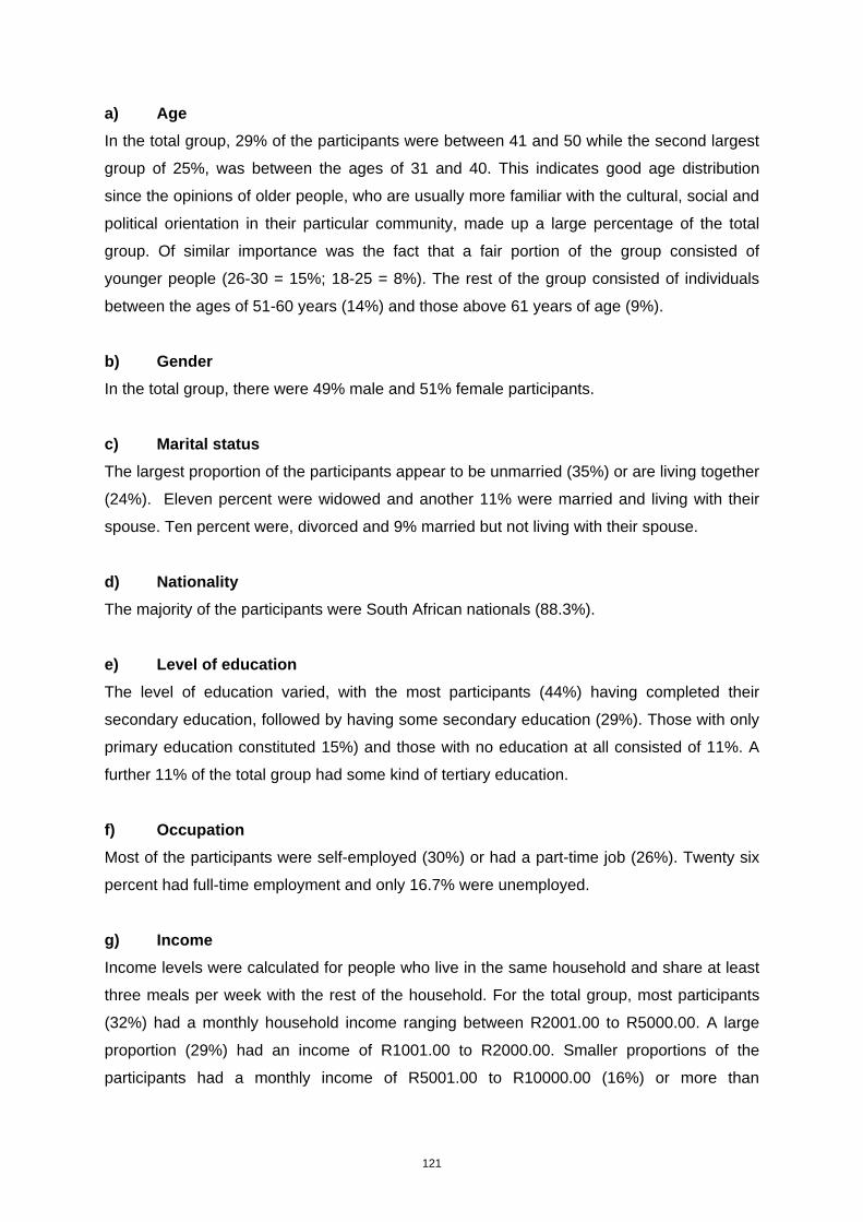
121

a) Age

In the total group, 29% of the participants were between 41 and 50 while the second largest

group of 25%, was between the ages of 31 and 40. This indicates good age distribution

since the opinions of older people, who are usually more familiar with the cultural, social and

political orientation in their particular community, made up a large percentage of the total

group. Of similar importance was the fact that a fair portion of the group consisted of

younger people (26-30 = 15%; 18-25 = 8%). The rest of the group consisted of individuals

between the ages of 51-60 years (14%) and those above 61 years of age (9%).

b) Gender

In the total group, there were 49% male and 51% female participants.

c) Marital status

The largest proportion of the participants appear to be unmarried (35%) or are living together

(24%). Eleven percent were widowed and another 11% were married and living with their

spouse. Ten percent were, divorced and 9% married but not living with their spouse.

d) Nationality

The majority of the participants were South African nationals (88.3%).

e) Level of education

The level of education varied, with the most participants (44%) having completed their

secondary education, followed by having some secondary education (29%). Those with only

primary education constituted 15%) and those with no education at all consisted of 11%. A

further 11% of the total group had some kind of tertiary education.

f) Occupation

Most of the participants were self-employed (30%) or had a part-time job (26%). Twenty six

percent had full-time employment and only 16.7% were unemployed.

g) Income

Income levels were calculated for people who live in the same household and share at least

three meals per week with the rest of the household. For the total group, most participants

(32%) had a monthly household income ranging between R2001.00 to R5000.00. A large

proportion (29%) had an income of R1001.00 to R2000.00. Smaller proportions of the

participants had a monthly income of R5001.00 to R10000.00 (16%) or more than

122

R10000.00 (6%). Less than 9% of the participants had income of less than R1000.00 per

month.

h) Number of dependants

Most of the participants (46%) had one or two dependants. Twenty two percent had, three

dependants, 18% had no dependants and a further 18% had four or more.

6.2.3 Procedure

A list with the contact details for ward councillors in each municipal area was obtained during

the qualitative phase from their respective local municipal offices. First contact with the

participants was made by means of a general telephonic conversation. The aim of this

conversation was to determine each participant’s willingness to take part in the research, to

inform him/her about the broad objectives of the study and to discuss the nature and

duration of his/her participation, should the participant agree to take part in the research.

Meetings were then scheduled for face-to-face interviews and focus groups with participants

(at a time and place most convenient to each of them) during which the details of the study

were discussed before participants were asked to tell the researchers about their community

and, more specifically, their interactions with water in their particular community.

During the quantitative phase, local community members were recruited as fieldworkers and

trained in the questionnaire and on how to conduct a community survey. In proclaimed areas

where street names and numbers are present, the sample was pre-planned (systematically

conducted and proportionately allocated according to the number of households in each

community). In unproclaimed areas, the number of households was first counted, the sample

proportionately allocated (according to its size) and then systematically conducted.

6.2.4 Data gathering methods

Three data gathering methods (de Vos et al., 2007) were used during the qualitative phase,

namely in-depth interviews with key informants, focus group discussions and observations.

All verbal data (interviews) were tape-recorded and transcribed to ensure accuracy. To

ensure validity in the qualitative findings, Guba’s model of trustworthiness (Kreftin, 1991),

consisting of four criteria (credibility, transferability, dependability and confirmability), was

applied using strategies proposed by Shenton (2004). A research questionnaire (Appendix

2) was then developed and used in a survey of the communities.

123

In-depth interviews: Face-to-face interviews were conducted with each participant, because

of their usefulness for gathering data in a person’s own, verbalised words. A benefit of using

interviews as a data gathering method is that it permits immediate follow-up questions that

can be used for clarifications. They can therefore be regarded as a flexible mode of data

collection that not only contributes to the trustworthiness of the data but the general

credibility of the study. Open-ended questions were used to ask participants to share

information about their community (interactions with water).

Focus group discussions: Small groups of between two and five participants were asked to

express their opinions on a specific set of open-ended questions regarding the community in

general, as well as their community’s interactions with water. Focus groups are more cost-

and time effective than individual interviews.

Observations: General non-participant observations/field notes were made in each

community to supplement or support the data generated by interviews and to ensure that the

results of the study were context specific.

During the quantitative phase (community survey), a consent form (Appendix 1), a page

consisting of eight demographic questions and a semi-structured questionnaire were

developed for use in the second phase of the research (Appendix 2). The demographic

questionnaire was used to collect basic demographic/background information (age, gender,

marital status, nationality, level of education, occupation, average household income per

month, number of dependants in household).

6.2.5 Data analysis

Thematic content analysis was used to analyse the verbal data during the qualitative phase.

Each transcribed text was first read and studied in detail to gain a broad overview of the

data. Units of meaning, including sentences or paragraphs relating to the topic, were then

identified in each of the texts and coded accordingly. This was followed by grouping related

units of meaning under a descriptive theme. Each theme was then again carefully studied in

detail to check that the original data truly supported the theme identified as well as to identify

the units of meaning and links with other themes.

The statistical consultation services of the North-West University were used for the statistical

analysis in this study. Descriptive statistics, including frequency tables, were calculated for

all themes and subthemes in each community and also for the weighted population of the

total group. Crosstabs and Cramer’s V test was used to determine if there were any

124

statistical or practical differences between the two districts. Statistical significant differences

are indicated by p < 0.05, with 0.10 indicating a small difference, 0.30 a medium difference

and 0.50 a large difference (that is practical significant). Cramer’s V becomes significant at

0.25.

6.3 Qualitative results

Five different themes emerged in relation to the interactions of communities with water.

Table 44 indicates these themes and the subthemes that emerged and gives verbatim

examples to support each theme or subtheme.

Table 44: Overview of qualitative results.

Theme Subtheme Verbatim example

Perceptions

about water

Quality

Availability

Management

“Here in our village water is scarce, but very

good. We drink it. Our livestock drink it. No

problem.”

“Water is a scarce resource and it must be

conserved”

“Sometimes we have problems, but in

general there is no problems”

Beliefs/attitudes

towards water

Water should be free

Spiritual and cultural

connections

“We all need water. Us humans and our

livestock. It is government’s responsibility”

“Water is very important to our people

(culture)”

Sources of

water

(most came up with a list)

Uses of water Physical (physiological)

needs

Everyday household use

Recreational purposes

Religious/spiritual and

cultural purposes

“In our community we can fish for food and

we drink the water every day”

“We use it for everything, from washing to

cooking and building”

“The small children swim here (pointing to a

small pond) after school”

(same as under beliefs)

125

Water

management

“Now we are lucky. In the past we used to

walk far. Now we have a tap in the yard”

6.3.1 Perceptions about water

Quality: The quality of water according to most participants refers to aspects such as the

colour (cleanliness and brightness), smell and composition (if there are debris of plants or

animal material) of their water. Perceptions of the quality of water in each community varied

considerably from poor to very good or excellent. One of the participants captured the

general opinion of the group very well when he said: “Here in our village water is scarce, but

very good. We drink it. Our livestock drink it. No problem”, while a small group of participants

in another community said: “We don’t like the water here. It is not good.”

Availability: In some of the communities in the Dr. Kenneth Kaunda District, participants

often commented on the availability of water, including that it is freely available compared to

communities in the Bophirima District where it was often said that “water is a scarce

resource and it must be conserved”.

Management: Most participants thought that their water resources were managed effectively

and optimally by local and provincial authorities. Most participants said that they do

“encounter problems every now and then” but, in general, they can’t complain.

6.3.2 Beliefs about and attitudes towards water

Water should be free. Participants often referred to water as a “shared resource” that should

be available free of charge. In other words, that no person should be expected to pay for

water and that it is government’s prerogative to provide people with water and for other

water-related uses such as sanitary purposes. One participant made this clear when he said:

“We all need water. Us humans and our livestock. It is government’s responsibility.”

Spiritual and cultural connections: Many participants indicated that they or “the people of

their community” have a strong spiritual connection with water. They therefore use water in

rituals or ceremonial acts to cleanse themselves/others, for example after a funeral, or to get

in contact with their ancestors. One participant said it best when he noted that: “Water is

very important to our people (culture). We use it to make contact with our ancestors. We also

use it to wash people before church or after a funeral.”

126

6.3.3 Sources of water

A number of sources of water were indicated in each community, including by pumping

water from a borehole/well (e.g. draw-well, pit, etc.) with a windmill or an electrical pump

(motor), by collecting rain water (rain harvesting) or by obtaining water from a cave or

underground source (Tigane), dam, fountain, pan (seasonal or permanent) or river or by

making use of municipal water (“tap water”).

6.3.4 Uses of water

Physical (physiological) needs: Participants use water for a variety of reasons related to

physical needs, for example to drink on a daily basis, to fish in, or to harvest plants/other

edible creatures (for food). One participant described it best when he said: “In our

community we can fish for food and we drink the water every day.”

Everyday household use: According to the participants, water for everyday household use

includes using it to build, by using a mixture of soil and water (mud) for building or

construction purposes (e.g. houses), for cooking food, to flush their toilets, to give to their

livestock (to drink), to grow/water crops (larger scale farming), wash their clothes in, to wash

goods (cleaning of physical objects other that themselves), to wash themselves (bath) or

their hands before or after eating, to water their gardens (domestic plants) and for example

to water their vegetables (on smaller scale/for subsistence). One participant summarised it

when she said: “We use it for everything, from washing to cooking and building.”

Recreational purposes: Participants, especially the youth in their communities, use water for

swimming and/fishing (recreational purposes). This appears to be more common in the rural

areas, especially in Bophirima. A teacher from one of the schools confirmed this when he

said that: “The small children swim here (pointing to a small pond) after school.”

Religious/spiritual and cultural purposes: This includes the use of water to wash their/other’s

feet before church or to wash themselves/others after a funeral service, the use of water to

drive out evil spirits/to remove evil spirits (cleansing themselves/members of their family or

house), to help them when they are fasting, to initiate a traditional healer/s in their

community or to make traditional medicine (to steam, drink or mix with other herbs, etc.), and

for example to make traditional beer (umqhombothi).

6.3.5 Water management

The theme water management includes how water is obtained and managed after it has

been obtained. For example, one of the participants said: “Now we are lucky. In the past we

127

used to walk far. No we have a tap in the yard.” It the past, people often had to travel large

distances to get water. Nowadays, in most cases, it appears as if they get most of their water

directly from a tap in the house/homestead, or from a tap in their yard, or by using a

communal tap for which they have to walk a distance of between less than 50 m from

homestead to larger distances of more than 50-100 m. Some communities experience water

shortages (from time to time) or lack infrastructure and therefore have to depend on water

that is delivered to them by a water tank/truck. Once the water is obtained, it is generally

either stored in a container in the house where it may be cooled down (e.g. by keeping it in a

fridge) or it is simply kept in a container outside the home.

6.4 Quantitative results

Results for the total group are reported, except where there was a significant statistical or

practical difference between the two districts. (All y-axis are percentages).

a) Perceptions about water

Figure 37: Perceptions about water quality.

There were no meaningful differences between the two districts regarding their perceptions

about the quality of their water or its availability. The majority of the participants perceived

the quality of their water to be average (72%), while 25% thought that their water is of good

quality. A small percentage (0.5%) thought that their water is of very good or excellent

quality and only 2.5% that it is of poor quality (Figure 37).

0

10

20

30

40

50

60

70

80

Poor Average Good Very good/excellent

128

Figure 38: Perceptions related to the availability (scarce resource) and management of

water.

The majority of the participants in each of the two districts perceives their water to be a

scarce resource (Dr Kenneth Kaunda district = 84.6%; and Bophirima district = 85.2%) but

differed in their opinion regarding how their water is managed (Figure 38). In Bophirima,

almost half of the participants (47%) said that they think their water is not managed correctly,

while the majority of participants in Kenneth Kaunda (72%) thought their water is managed

correctly (p < 0.05; Cramer’s V = 0.20).

b) Beliefs about and attitudes towards water

Figure 39: Beliefs and attitudes towards water.

0

10

20

30

40

50

60

70

80

90

Availibility Management

Total group

Dr. KK

Bophirima

0

20

40

6080

100

120

Water should befree

Conserved Spiritual connection Self cleancing afterfuneral

Contact withancestors

Total group

129

Ninety percent of participants felt that they should not have to pay for water. A larger

percentage (97%) felt that water must be used sparsely or should be conserved. Forty

percent of the participants (said that they have a spiritual connection with water. A large

percentage (75%) indicated that they use water for example to cleanse themselves or others

after a funeral or burial ceremony. Forty five percent use water to make contact with their

ancestors (Figure 39).

c) Sources of water

Figure 40: Sources of water (1 = Borehole with a windmill; 2 = Borehole with an electrical

pump (motor); 3 = By collecting rain water; 4 = Cave or underground source; 5 = Dam; 6 =

Fountain; 7 = Municipal water (tap); 8 = Pan (seasonal or permanent); 9 = River; 10 = Well

(e.g. draw-well, pit, etc.)).

The majority of households (76.5%) make use of municipal water. Sources of water did not

differ greatly between the two districts, except in regard to the harvesting of rain water. In the

Bophirima district, more of the participants make more use of rain water harvesting (32.3%),

compared to the Dr Kenneth Kaunda district (32% vs. 11%). Other sources of water include

boreholes with windmills (21%), or borehole with electrical pumps (10%), seasonal pans

(6%), fountains (5%), dams and rivers (4%) as well as wells (4%) (Figure 40).

0

20

40

60

80

100

1 2 3 4 5 6 7 8 9 10

Total group

Bophirima

Dr. KK

130

d) Uses of water

Figure 41: Uses of water (1 = Build our house/other physical structure (for example in

combination with mud); 2= Cleanse myself/ourselves from the inside (enema); 3 = Cook

my/our food; 4 = Drink (when I am/we are thirsty); 5= Drive out evil spirits/to remove evil

spirits (cleansing myself/members of my family or house); 6 = Flush my/our toilet; 7 = Give to

my/our livestock (to drink); 8 = Help me when I am fasting; 9 = Initiate the traditional healer/s

in our community; 10 = Make traditional medicine (to steam, drink, or mix with other herbs,

etc.); 11 = Swim or fish in (recreational purposes); 12 = Fish in, to harvest plants from or

any other edible creatures (for food); 13 = Grow/water crops (larger scale farming); 14 =

Make traditional beer (umqhombothi);15 = Wash my clothes in;16 = Wash my/other’s feet

before church;17 = Wash my/our goods (cleaning of physical objects other that myself); 18 =

Wash myself (bath); 19 = Wash myself/others after a funeral service; 20 = Wash my/our

hands; 21 = Water my garden (domestic plants); 22 = Water my vegetables (on smaller

scale/for subsistence)).

The number of uses of water differed statistically and practically between the two districts

(Figure 41). When comparing the Bophirima and Dr Kenneth Kaunda districts the following

pattern emerges:

• traditional uses such as using water to drive out evil spirits or to remove evil spirits

(cleansing themselves or members of their family or house) (75% vs. 50%; p < 0.05;

Cramer’s V = 0.25)

• making traditional medicine (to steam, drink, or mix with other herbs, etc.) (81% vs.

56%; p < 0.05; Cramer’s V = 0.26),

• swim or fish in (recreational purposes) (75% vs. 54%; p < 0.05; Cramer’s V = 0.21)

0

20

40

60

80

100

120

1 2 3 4 5 6 7 8 9 10 11 12 13 14 15 16 17 18 19 20 21 22

Total group

Bophirima

Dr. KK

131

• to fish in (to harvest plants from or any other edible creatures (for food) (43% vs.

20%; p < 0.05; Cramer’s V = 0.25) and

• livestock watering (70% vs. 28%; p < 0.05; Cramer’s V = 0.41).

Other popular uses of water that 88% more of the participants mentioned include

the use of water for house building or other physical structures (for example in combination

with soil) (94%),

• to cook their food (99%), to drink (98%),

• to flush their toilet (96%),

• to help them when they are fasting (92%),

• to wash their clothes (99%),

• to wash their brother’s feet before church (97%),

• to wash their goods (cleaning of physical objects other that themselves) (99%),

• to wash themselves (bath) (98%),

• wash their hands (99%) and

• to water their garden (domestic plants) (93) and to make traditional beer

(umqhombothi) (88%).

Other uses of water include:

• self-cleansing (enema) (68%),

• to initiate the traditional healer/s in their community (75.9%),

• larger scale farming (grow/water crops) (27.8%),

• to wash themselves or others after a funeral service (62.9%) and

• to use water for smaller scale/subsistence farming (to grow vegetables (69.8) (Figure

41).

e) Water management

Figure 42: Water availability and management.

020406080

100120

In house Tap in yard Communal tap Travel large distance Delivered

Total group

132

The majority of households (97%) appear to make use of a tap in their yard even though

45% have water in their houses. Very small percentage of participants use a communal tap

(4%) for which they have to travel less than 50 meters. Two percent have to fetch water

more than 50 meters from their dwelling and another 2% gets water that is delivered to them

(Figure 42).

Figure 43: Storage and management of water.

Most households appear to store water inside their homes (64.5%) where it is cooled down

in most cases (82.9%). Communities in the Bophirima district tend to store water more

regularly in containers outside their house compared to the Dr Kenneth Kaunda district

participants (56% vs. 34%; p < 0.05; Cramer’s V = 0.30; Figure 43).

6.5 Discussion and conclusion

From the findings it is clear that people’s interactions with water elicit certain perceptions,

beliefs and attitudes and behaviours (e.g. uses of water, water management, etc.). There

were, however, no meaningful differences between people’s (i.e. the different communities’)

perceptions regarding the quality of their water. This is something that is subjective and it will

be interesting to compare this to actual water quality data in the different communities. The

management and availability of water are more objective, because it is something that is

experienced by the communities on a daily basis. The good news is that people in these

communities appear to realise that water is a scarce resource and that it should be

conserved and used sparsely. In terms of future interventions, there is, therefore, no need to

start education or awareness campaigns in these communities. Education programmes

could build on the existing knowledge and understanding of community members.

There were, however, differences regarding people’s perceptions about how their water is

managed. This is something that needs to be taken up with local authorities, where they can

come up with better strategies to involve the local communities in their planning. A good

0102030405060708090

Container in house Container outside house Cool down

Total group

Bophirima

Dr. KK

133

public participation process will make the people from these communities feel more involved

or will at least sort out misperceptions if they exist.

One aspect that people felt very strongly about is that they should not be expected to pay for

water. Water is often regarded as a shared resource that should be respected, but

something that belongs to everyone. It is no surprise in a democratic country such as South

Africa that people are aware and willing to stand up for their basic rights, like in this case free

access to water. The South African government currently provides a certain amount of water

free to all the people of South Africa (ANC freedom charter), but the amount of free water is

often considered insufficient for everyday household use. From the results it is evident that

the average number of dependants per household is small. It could thus be argued that due

to this average households should have sufficient free water. Government has also come a

long way to provide access to water, to households. However, this study has shown that

most households make use of a tap in their yard. Similar results were found by Coetzee and

Du Toit (2011) in the rest of the province.

An interesting result is that there are differences between communities regarding the

harvesting of rainwater. More people in communities in Bophirima district tend to harvest

water compared to people living in communities in Dr. Kenneth Kaunda district. Water is a

scarce resource and education and awareness programmes related to water harvesting in

the Dr. Kenneth Kaunda district will definitely help to provide and use water in the district in a

more sustainable manner.

Other interesting results are the fact that a significant number of people in the communities

that were surveyed still make use of borehole water that is powered by a windmill. This is

presumably as a secondary source of water but it needs to be confirmed whether or not

community members consider this as the provision of water from local government. It also

opens up the possibility to introduce more sustainable sources of water provision and even

ways to generate energy in communities in the NWP, seeing that there is no shortage of

sunshine and wind. If added up, it also appears as if a significant number of people in the

province, especially in rural areas, still use natural sources of water such as pans, dams and

rivers to get water. This makes them vulnerable to water pollution and the associated risks

that go with it (Beekman, 1998)

In general, the uses of water appear to be similar in most communities and compare well

with more common uses documented in the literature (Coetsee, 2011). Some uses such

134

using water for transportation was not found, because the North West Province has very few

permanent water bodies like rivers.

In order to answer the rest of the second research question, it was found that some uses of

water differed significantly between the communities, for example uses of a more cultural

nature, e.g. to drive out evil spirits/to remove evil spirits (cleansing themselves/members of

their family or house) and to make traditional medicine. The use of traditional medicine is not

always common knowledge especially in more urban areas where traditional knowledge is

often lost due to acculturation (people becoming more westernised) and enculturation

(knowledge not being transferred) (Reeder, 2011). This result can perhaps be explained by

the fact that the two communities in the Bophirima district are more rural compared to the

semi-urban communities in the Dr. Kenneth Kaunda district and the aforementioned

reasons. Furthermore, rural communities also often have different values than people in

more urban areas (with a different set of social and political dynamics) which could explain

why children tend to swim or fish more for recreational purposes or to harvest plants or other

edible creatures from it. People in rural areas also tend to keep more livestock due to the

availability of communal grazing areas.

Finally, the quantitative results confirmed that most people in the communities that were

surveyed have a strong spiritual and cultural connection with water. Some of the more

spiritual and cultural interactions that people have with water, in terms of uses, include the

use of water to wash themselves before and after funeral services. This is presumably as a

sign of respect for the deceased. It is something that is prominent in many African cultures

(Reeder, 2011). This is an aspect that needs further exploration if culture sensitive

interventions need to be developed in future.

In conclusion, this study has shown that people interact with water in various ways and that

certain perceptions, beliefs and behaviours are associated with these interactions. It has

also shown that water has important social and cultural meanings to people and also the

biggest difference when communities from Dr. Kenneth Kaunda are compared to Bophirima.

Finally, although the study has limitations, in general, it provides an excellent platform for

future research and interventions in the province.

6.6 Limitations

• The biggest limitation is that, due to funding and other restraints, not more

communities could be included in the research. Six out of a potential 50 communities

(own estimate) could be included. The communities that were included do, however,

135

appear to be fairly representative in terms of general size and structure and

dynamics when compared to other communities in the province.

• Other limitations include the fact that this is an ad hoc study and it is a pity that more

social-orientated studies are not done in the province.

• A final limitation is the fact that the current project does not allow a report back to all

the communities that were surveyed to share with them what has been learned.

6.7 Recommendations

• A study to compare the perceptions of the six communities that were included in this

study of the quality of their water to the actual water quality should be conducted. In

the present study the actual water quality of the communities were not determined.

Actual microbiological and physico-chemical quality data would provide insights into

the perception of the community members. This study on water quality perceptions

and actual water quality should then be repeated in new communities that were not

previously included.

• A study to confirm the amount of water needed by communities on a household level

per day should also be conducted. This should be done over a larger number of

communities particularly those on rural and peri-urban areas. In the present study

most of the communities were in reasonable close proximity of potable water

sources. This could be accepted as the norm for the North West Province.

• More in-depth research on the spiritual and cultural connection that people have with

water in this province is needed. Some interesting uses of water with regards to

religious, traditional and cultural practices were mentioned by some of the

participants. There could be other uses as well such as full-body baptisms of adults

that were not mentioned. A study that focuses on these aspects should provide a

more in-depth knowledge of the association the people of the North West Province

and water.

• A study to determine the perceptions of the urban populations of the North West

Province on water quality, quantity interactions and management of water should

also be done. This was not initially part of the current study but this part of the

provincial population should be included in future studies.

• Study to investigate the feasibility of providing alternative water sources and sources

of energy (e.g. to pump or manage water) to communities should be conducted. For

example a programme in the harvesting of rain water should be considered. The

province is in a summer rainfall region and large quantities of water could be

136

harvested during this period. This water could then be used for various purposes

during the dry winter period.

137

CHAPTER 7

CONCLUSIONS AND RECOMMENDATIONS

7.1 CONCLUSIONS

The overall purpose was to conduct a large-scale study of microbial and physico-chemical

quality of groundwater and surface water in the North West Province, South Africa and to

provide a report of the results. The following conclusions were drawn from the results:

• Target water quality range comparisons (DWAF, 1996) of physico-chemical

parameters of selected surface water sources indicated that this water was generally

suitable for several uses including recreational and domestic uses. In some cases

electrical conductivity was elevated but not to an extent where negative health

implications would be associated with the consumption of the water. This elevated

EC could be indicative of increasing salinisation.

• Enterococcus spp. as well as Escherichia coli, were isolated demonstrating that the

specific surface water sources are contaminated by various faecal indicator bacteria.

Several of the enterococci species identified are potentially pathogenic to humans

and animals. A very small percentage of E. coli isolates were entero-pathogenic

strains and could have human and animal health implications.

• Candida, Clavispora, Cryptococcus, Cystofilobasidium Hanseniaspora, Meyerozyma,

Pichia, Rhodotorula, Saccharomyces, Sporidiobolis, and Wickerhamomyces are

various yeast genera that were isolated. Some these species of these genera may

cause invasive infections in sensitive individuals.

• Baseline culture independent molecular profiling data of the dominant bacterial

communities in the Vaal River were also provided by DGGE and HTS profiling.

These methods allowed for the identification of the bacterial community composition

and dynamics in the planktonic component in this river system. Next generation

sequencing or (HTS, high through-put sequencing) analysis presented a better

resolution of the bacterial diversity and dynamics in the Vaal River compared to

DGGE.

138

• The bacteriophage data supported the general findings of the bacterial analysis i.e.

that many of the water sources in the North West Province have some form of faecal

pollution. Phages were also isolated from potable water sources and this is a cause

for concern.

• Boreholes that were sampled generally complied with the drinking water TWQR

(DWAF, 1996) accept for nitrates. Less than 30% all boreholes tested complied with

<6 mg/ℓ NO3N for drinking water (DWAF, 1996). Some of the levels were greater

than 400 mg/ℓ NO3-N. Such high levels of nitrates could have human health

implications.

• Faecal contamination of the groundwater was demonstrated by data from indicator

bacteria, bacteriophage and faecal sterol data. In addition to bacterial faecal

indicators, P. auruginosa and Staph aureus were also found in many borehole water

samples. Next generation sequencing (or high through-put sequencing) results

provided supported the culture dependent data.

• Animal species-specific faecal sterol profiles were generated using the Szuc method.

This method demonstrated the potential of using such an approach in source tracking

faecal pollution in the North West Province for local application.

• Another potential application of the faecal sterol analysis is to use it to evaluate the

efficiency of wastewater treatment plants. However, more accurate sterol recovery

methods and larger sample volumes needs to be considered (Leeming, 2006) and

the method optimised and validated.

• Sterol analysis may also aid in the water quality determination of both ground- and

surface water. It can is used to determine the source of faecal pollution by utilising

the faecal sterol ratios.

• Culture independent methods (PCR-DGGE and HTS) supported groundwater

bacteriological plating results for faecal indicator bacteria. Additional pathogenic and

potential pathogenic species were also identified by these methods.

• The results indicated that several human pathogens as well as opportunistic yeast

pathogens were present in the water sources. Enterovirus (qPCR) analysis

139

demonstrated that WWTPs may be decanting large amounts of this (and potentially

other viruses) into receiving water bodies if poorly or untreated sewage is allowed

into such water sources.

• Results of a cytotoxicity test developed during this study demonstrated that such a

test could act as a first tier evaluation of the potential of water for negative health

impacts. Once refined it could be a useful system for a widespread application to

water in the North West Province and elsewhere. All flagged samples could then be

further investigated for the actual causes of cytotoxicity.

• The social and water management part of the study has shown that people interact

with water in various ways. It also demonstrated that certain perceptions, beliefs and

behaviours are associated with these interactions. It was demonstrated that water

has important social and cultural meaning. Responses from people in the

communities surveyed indicated that they realise that water is a scarce resource and

that it should be conserved and used sparingly.

7.2 RECOMMENDATIONS

• Microbiological and physico-chemical quality of drinking-water boreholes should be

combined with epidemiological studies to determine how many water users served by

these groundwater sources become ill each year as a result of using this source. The

present study, as well as previous ones, has demonstrated that several of the

surface waters and groundwater sources are polluted by faecal matter. These results

have indicated that nitrate concentrations are high in some areas. However, no

epidemiology data is available to demonstrate conclusively that the pollution is linked

to disease burden. Disease states should include diarrhoea, physiological conditions

as well as skin and invasive infections. A study that is focused on the nitrate

concentrations in groundwater of the North West Province should also be conducted.

The geology of the area, depth of the boreholes, rainfall events, fertiliser application

rates and the proximity of the boreholes to agricultural lands and human settlements

should be considered.

• Another aspect that needs to be addressed is the elevated electrical conductivity that

was observed at several of the sites. Sources of these high EC values should be

investigated as this could have serious implications on soil quality in the province and

by implication also food security. The North West Province is one of the main grain

140

producers in the country producing a large percentage of maize and sorghum,

amongst others. In many cases these crops are under irrigation. Salinisation of soils

will reduce the carrying capacity thereof and eventually render it unproductive. In

regions of the Vaalharts irrigation scheme, salinisation of soils has resulted in large

sections becoming waterlogged which are now completely unproductive. This could

also happen in the North West Province if early interventions are not put in place.

Elevated electrical conductivity will also impact negatively on livestock production. If

environmental water salt levels become such that additional treatment is required

then this will add cost to such operations. This will also have impacts on food

affordability and security. Continuously increasing EC will eventually also impact on

drinking water production in the process will add costs to drinking water. Although

elevated electrical conductivity does not appear to be a threat at the moment, it

should be carefully monitored, sources of the increases identified and appropriately

managed.

• Boreholes should be identified that may be vulnerable to certain types of

contamination. Site-specific conditions such as soil properties, vegetation, and

topography may affect contaminant transport at boreholes. Various sources could

further contribute to nitrate contamination of boreholes. These include the geology,

agricultural practices such as high density feed lots, use of un-composted faecal

material as well as fertiliser remnants in soil. Some of the factors and sources

mentioned could contribute to high levels of nitrates and faecal matter in groundwater

in the North West Province (NWP-SOER, 2002). Causes of contamination of

groundwater should not be generalised and specific ones affecting specific boreholes

investigated. Large sections of the rural communities in the North West Province are

dependent on groundwater for all their domestic needs. Thus when groundwater is

supplied to communities and schools in this province, a detailed analysis of the water

quality should be conducted. Regular tests should also be done by the supply water

authorities to ensure that the water is of suitable quality for the intended use. In

cases where the nitrate and electrical conductivity levels are high purification steps

should be considered. These boreholes should be sampled and analysed on a

regular basis. During every sample event, the surrounding area, human and

environmental influences as well as seasonal variables should be recorded. This will

allow for insights into the factors promoting the contamination of the groundwater and

preventative or remedial processes could be put in place.

141

• Future studies to determine the presence of E. coli and other indicators in the water

should be conducted also using PCR methods instead of only culture based

methods. The latter methods are tedious and confirmation of identities takes several

days. False negative results are a cause for concern particularly if pathogenic E. coli

may be present in the samples. PCR methods will only give qualitative results i.e.

present or absent but results will be available in a much shorter time frame than what

is feasible with culture dependent methods. Also, quantitative analyses may be

achieved using real-time PCR technologies. Reverse Transcription-qPCR may be

useful to distinguish between viable and non-viable bacteria. PCR based methods

allow for a faster turnaround time of results and may provide more accurate results

than the traditional culture based methods.

• The traditional culture based methods provided microbiologists with a number of

organisms that could be used to indicate pollution events. Such methods mainly

focus on the microbial quality of water for specific uses. The methods also do not

have sufficient resolution to provide insights into the important ecological processes

occurring within aquatic ecosystems. This is because cultivation procedures allow for

a small number of microbes to be cultivated. Estimating the total microbial diversity

and identifying microbial assemblages as well as proposing their role at community

level is thus not possible. Understanding the microbial community dynamics in

aquatic systems may provide microbiologists with better approaches to determine

and predict the effects of pollution. Since organisms normally act within in

communities their abundance will then be dependent on the selection forces

prevailing within the community and environment. In the present study two culture

independent approaches demonstrated that the traditional indicator bacterial species

were not detected in large quantities. Both these approaches found various other

bacterial phylogenetic groups present of which some uncultured species were

previously detected in aquatic ecosystems. Future work in this regard is thus

necessary. It should concentrate on in-depth HTS analysis of the microbial diversity

and water quality in the surface and groundwater with the focal point on the

identification of specific species within the major key groups. Identification may

phylogenetically affiliate uncultured bacteria with known bacterial genera or species.

It may thus be possible to cultivate some of these previously uncultured bacteria

using specific nutrient, pH and temperature conditions. Morphological descriptions

may then be possible. Such species may then be further exploited as indicators

species of specific pollution event

142

• Further research into the levels and diversity of yeasts in the North West Province

should be conducted. Their potential sources should also be investigated. The

association of yeast and organic carbon pollution should also be investigated. What

also needs to be determined is an equivalent level of risk of illness. There is

presently no regulation or risk model for yeasts in aquatic ecosystems. The various

yeast genera and species identified in the present study are mostly associated with

opportunistic infections in immune-compromised. Cryptococcus neoformans is one

species of particular concern. However, in the present study a species that causes

the same symptoms as C. neoformans was isolated. The levels and distribution of

this species is unknown. There may also be other species that are of clinical

importance that could be present in the water source of the North West Province.

This is against the back drop of numerous waste water treatment plants in the

province not operating optimally and in many of these cases, untreated sewage is

allowed to enter waterways. In the present study the number of sampling sites and

isolates identified were limited. A large-scale study should be designed particularly

around the areas that are most frequently used by the community of the North West

Province for full contact activities. This will provide clearer insights into the actual

infection risks of exposure to the various yeast species.

• A need exists to gain more knowledge about the social context and management of

water at a community level in the North West Province. In the present study rural and

peri-urban communities were targeted. Future studies should include urban

communities a larger cross section to include all the economic groups. Such a study

should also include a section of the water needs and efforts that community

members make to conserve water. More in-depth research on the spiritual and

cultural connection that people have with water should also be considered. A study to

investigate the feasibility of providing alternative sources energy to pump (or

manage) water to communities. Education and awareness programmes to promote

the harvesting and use of rain water should also be considered, particularly for the

western part of the province that borders on and is part of the Kalahari Desert. It is

imperative that communities are made aware of, and understand the risks involved

with using untreated groundwater as a source for domestic purposes. By having

knowledge of the water quality they use, communities should be encouraged to treat

the water at household level (boiling of water, point-of-use chlorination, UV treatment

and safe storage practices). These practises will aid in the prevention of waterborne

diseases. Education on the routes and sources of contaminants should also

encourage communities to take ownership of their health.

143

REFERENCES

Achleitner S., DeToffol S., Engelhard C., Rauch W. (2005). The European Water Framework

Directive: Water Quality Classification and Implications to Engineering Planning.

Environmental Management, 35 (1), 1-9.

Adeleke, R., Bezuidenhout, C.C. 2011a. Integrated Water Resources Management (IWRM)

in South Africa –Challenges of Microbiology quality of water resources. African Journal of

Science Technology Innovation and Development, 3(4) 55-64

Adeleke, R., Bezuidenhout, C.C. 2011b. Detection of high levels of enteric viruses in some

treated sewage water from the Northwest Province. South African Society for Microbiology,

Cape Town, 6-9 November

Al-Khatib, I.A., Arafat, H.A. 2009. Chemical and microbiological quality of desalinated

water, groundwater and rain-fed cisterns in the Gaza strip, Palestine. Desalination, 249(3),

1165-1170.

Allen, M.J., Reasoner, J., Edberg, S.C. 2004. Heterotrophic plate count bacteria – What is

their significance in drinking water? International Journal of Food Microbiology, 92: 265–

274.

ANC Freedom-charter: http://www.marxists.org/subject/africa/anc/1955/freedom-charter.htm

(accessed 30 April 2012)

Anon. 2007. Cholesterol in your body. http://www.prolipid.com/background-

articles/cholesterol-in-your-body.html (accessed 26 May 2011).

Anon. 2009a. The water project. The Water Project, Inc. is a public charity under Section

501(c) (3) of the Internal Revenue Code. [URL:

http://thewaterproject.org/water_scarcity.asp?gclid=CKnVgeG1 h54CFUQA4wodxleMoQ

Date Accessed: 10 November 2009]

Anon. 2009b. Case 1498/09 http://www.saflii.org/za/cases/ZANWHC/2009/17.pdf)

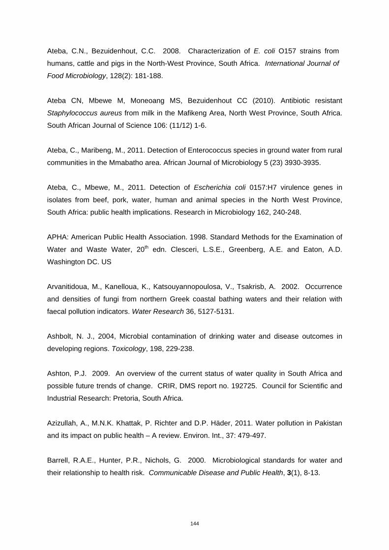
144

Ateba, C.N., Bezuidenhout, C.C. 2008. Characterization of E. coli O157 strains from

humans, cattle and pigs in the North-West Province, South Africa. International Journal of

Food Microbiology, 128(2): 181-188.

Ateba CN, Mbewe M, Moneoang MS, Bezuidenhout CC (2010). Antibiotic resistant

Staphylococcus aureus from milk in the Mafikeng Area, North West Province, South Africa.

South African Journal of Science 106: (11/12) 1-6.

Ateba, C., Maribeng, M., 2011. Detection of Enterococcus species in ground water from rural

communities in the Mmabatho area. African Journal of Microbiology 5 (23) 3930-3935.

Ateba, C., Mbewe, M., 2011. Detection of Escherichia coli 0157:H7 virulence genes in

isolates from beef, pork, water, human and animal species in the North West Province,

South Africa: public health implications. Research in Microbiology 162, 240-248.

APHA: American Public Health Association. 1998. Standard Methods for the Examination of

Water and Waste Water, 20th edn. Clesceri, L.S.E., Greenberg, A.E. and Eaton, A.D.

Washington DC. US

Arvanitidoua, M., Kanelloua, K., Katsouyannopoulosa, V., Tsakrisb, A. 2002. Occurrence

and densities of fungi from northern Greek coastal bathing waters and their relation with

faecal pollution indicators. Water Research 36, 5127-5131.

Ashbolt, N. J., 2004, Microbial contamination of drinking water and disease outcomes in

developing regions. Toxicology, 198, 229-238.

Ashton, P.J. 2009. An overview of the current status of water quality in South Africa and

possible future trends of change. CRIR, DMS report no. 192725. Council for Scientific and

Industrial Research: Pretoria, South Africa.

Azizullah, A., M.N.K. Khattak, P. Richter and D.P. Häder, 2011. Water pollution in Pakistan

and its impact on public health – A review. Environ. Int., 37: 479-497.

Barrell, R.A.E., Hunter, P.R., Nichols, G. 2000. Microbiological standards for water and

their relationship to health risk. Communicable Disease and Public Health, 3(1), 8-13.

145

Bai, J., Shi, X., Nagaraja, T. G., 2010, A multiplex PCR procedure for the detection of six

major virulence genes in Escherichia coli O157:H7 Journal Microbiological Methods, 82, 85-

89.

Batta A. K., Salen G., Batta P., Tint G. S., Alberts D. S., Earnest D. I. (2002). Simultaneous

quantitation of fatty acids, sterols and bile acids in human stool by capillary gas-liquid

chromatography. Journal of Chromatography B, 775, 153-161.

Bauer, A., Kirby, W.M.M., Sherris, J.C., Turck, M. 1966. Antibiotic susceptibility testing by

single disc method. American Journal of Clinical Pathology, 45: 493.

Baxter H., Harborne J.B., Mass G.P. (1999). Phytochemical Dictionary: A handbook of

Bioactive compounds from plants, 2nd edn. Taylor and Francis, London, pp. 2975.

Beekman, G.B. (1998): Water conservation, recycling and reuse. International Journal of

Water Resources Development, 14:3, 353-364.

Berg, G., Eberl, L., Hartmann, A., 2005. The rhizosphere as a reservoir for opportunistic

human pathogenic bacteria. Environmental Microbiology, 7 (11), 1673-1685.

Bezuidenhout, C.C., Mthembu, N., Puckree, T., Lin, J. 2002. Microbiological evaluation of

the Mhlathuze River, Kwazulu-Natal (RSA). Water SA, 28: 281-286.

Bezuidenhout, C.C., Prinsloo, M., Van der Walt, A.M. 2006. Multiplex PCR-based detection

of potential fumonisin-producing Fusarium in traditional African vegetables. Environmental

Toxicology, 21: 360-366.

Biswas, A. K. (2004). Integrated water resources management: A reassessment. Water

International, 29(2):248-256.

Breitbart, M., Hoare, A., Nitti, A., Siefert, J., Haynes, M., Dinsdale, E., Edwards, R., Souza,

V., Rohwer, F., Hollander, D., 2009. Metagenomic and stable isotopic analyses of modern

freshwater microbialites in Cuatro Ciénegas, Mexico. Environmental Microbiology, 11 (1),

16-34.

Brettar, I., Höfle, M.G. (2008) Molecular assessment of bacterial pathogens – a contribution

to drinking water safety. Current Opinion in Biotechnology 19: 274-280.

146

Calderon, R.L., Mood, E.W. 1991. Bacterial colonizing point-of use, granular activated

carbon filters and their relationship to human health (CR-813978-01-0). U.S. Environmental

Protection Agency.

Candela, M., Maccaferri, S., Turroni, S., Carnevali, P., Brigidi, P. 2010. Functional

intestinal microbiome, new frontiers in prebiotic design. International Journal of Food

Microbiology, 140, 93–101

Cardenas, E., Tiedje, J.M., 2008. New tools for discovering and characterizing microbial

diversity. Current Opinion in Biotechnology, 19, 544–549

Carducci, A., Morici, P., Pizzi, F., Battistini, R., Rovini, E. Verani, M. 2008. Study of the viral

removal efficiency in a urban wastewater treatment plant. Water Science and Technology,

58 (4), 893-897.

Carstens, A., Bezuidenhout, C.C. 2012. Evaluation of microbiological and physico-chemical

quality of water from selected DWA (Department of Water Affairs) monitoring boreholes in

the North West Province, South Africa. Water Institute of Southern Africa, Cape Town, 6-10

May

Cho J.C., Cho H.B., Kim S.J. 2000. Heavy contamination of a subsurface aquifer and a

stream by livestock wastewater in a stock farming area, Wonju, Korea. Environmental

Pollution, 109(1), 137-146.

Coetzee, H.C. 2009. Needs assessment conducted in the Dr. Kenneth Kaunda (Southern)

District, North West Province, South Africa. A North-West Living Lab Baseline Project.

Coetzee, H.C. & Du Toit, I. 2011. Community needs and assets in the North West Province:

A baseline study to guide future community engagement and interventions in the province.

Collins, M.D., Farrow, J.A.E., Jones, D. 1986. Enterococcus mundtii sp.nov. International

Journal of Systematic Bacteriology, 36(1), 8-12.

Committee on Metagenomics: Challenges and functional applications, National Research

Council of the National Academies. The new science of metagenomics: revealing the secrets

of our microbial planet. 2007. Washington, DC: National Academic Press.

147

Constitution of the Republic of South Africa Act. Act No. 108, December 1996. Government

Gazette No. 17678. Cape Town, South Africa.

Cowan, D., Meyer, Q., Stafford, W., Muyanga, S., Cameron, R., Wittwer, P., 2005.

Metagenomic gene discovery, past, present and future. Trends Biotechnology, 23, 321-329.

Craun, G.F., Greathouse, D.G., Gunderson, D.H. 1981. Methemoglobinemia levels in

young children consuming high nitrate well water in the United States. International Journal

of Epidemiolology, 10(4), 309-317.

Craun, G.F., Calderon, R. 1997. Microbial risk in groundwater systems: Epidemiology of

water borne outbreaks. In: Under the Microscope examining microbes in Groundwater,

AWWA Research Foundation, Denver, Colorado

Creswell, J.W., Plano Clark, V.L. (2007). Designing and conducting mixed methods

research.CA, USA: Sage Publications

Crowther, J. Kay, D. Wyer, M.D. 2002. Faecal-indicator concentrations in waters draining

lowland pastoral catchments in the UK: relationships with land use and farming practices.

Water Research 36, 1725-1734.

CSIR: Council for Scientific and Industrial Research. 2010. The impact of an unhealthy

environment on human health in South Africa

Csuros, M., Csuros, C. 1999. Microbiological examination of water and wastewater.

Florida: CRC press, 245p.

Currie, S.L. 2001. The implementation of an environmental decision-making support system:

the Mooi River catchment as a case study. Potchefstroom: PU vir CHO. (Dissertation –

D.Phil).

Dallas, H.F., Day, J.A. 2004. The effect of water quality variables on aquatic ecosystems: a

Review. Water Research Commission, Report no. TT 224/04.

Darwish, T., Atallah, T., Francis, R., Saab, C., Jomaa, I., Shaaban, A., Sakka, A., Zdruli, P.

2011. Observations on soil and groundwater contamination with nitrate: A case study from

Lebanon-East Mediterranean. Agricultural Water Management, 99(1), 74-84.

148

de Figueiredo, D.R., Ferreira, R.V., Cerqueira, M., Condesso de Melo, T., Pereira, M.J.,

2012. Impact of water quality on bacterioplankton assemblage along Cértima River Basin

(central western Portugal) assessed by PCR–DGGE and multivariate analysis.

Environmental Monitoring and Assessment, 184 (1), 471-485.

De Vos, A., Strydom, H., Fouche, C.B., Delport, C.S.L. 2007. Research at grassroots for

social and human service professions. Pretoria: Van Schaik Publishers.

Dikobe, B.T., Sithebe, N.P., Ateba, C.N. 2011. Detection of E. Coli Isolates in water from

Setumo Dam Mmabatho Area – North West Province, South Africa using mdh specific PCR

analysis. Journal of Human Ecology 36(1), 29-35.

DoH: Department of Health. 2006. Standard treatment guidelines and essential drugs list

for South Africa. National Department of Health: Pretoria. Web:

http://www.kznhealth.gov.za/edladult06.pdf [Date accessed: 20 October 2010].

Dorigo, U., Volatien, L., Humbert, J.-F. 2005. Molecular approaches to the assessment of

biodiversity in aquatic microbial communities. Water Research, 39, 2207-2218.

Dryden M.S. 2009. Skin and soft tissue infection: Microbiology and epidemiology.

International Journal of Antimicrobial Agents, 34(1), S1-S7.

Dryden M.S. 2009. Skin and soft tissue infection: Microbiology and epidemiology.

International Journal of Antimicrobial Agents, 34(1): S1-S7

Duncker, L.C. 2000. Hygiene awareness for rural water supply and sanitation projects.

Water Research Commission, Report no. 819/1/100. Pretoria, RSA

DWAF: Department of Water and Forestry. 1996a. South African water quality guidelines,

Volume 1: Domestic use, 2nd Ed. Pretoria, South Africa.

DWAF: Department of Water Affairs and Forestry. 1996b. South African water quality

guidelines, Volume 4: Agricultural use: Irrigation, 2nd Ed. Pretoria, South Africa.

DWAF: Department of Water Affairs and Forestry. 1996c. South African water quality

guidelines, Volume 2: Recreational use: 2nd Ed. Pretoria, South Africa.

149

DWAF: Department of Water and Forestry. 1996d. South African water quality guidelines,

Volume. 8: Field Guide, 1st Ed. Pretoria, South-Africa.

DWAF: Department of Water Affairs and Forestry. 1996e. South African water quality

guidelines, Volume 5: Agricultural use: Livestock watering, 2nd Ed. Pretoria, South Africa.

DWAF: Department of Water and Forestry. 1999. Report on the radioactivity monitoring

programme in the Mooi River (Wonderfontein Spruit) catchment. Institute for water quality

studies, Report no. N/C200/00/RPQ/2399. Pretoria, South Africa.

DWAF: Department of Water and Forestry. 2000. National Microbial Water Quality

Monitoring Programme – A First Report on the Identification and Prioritisation of Areas in

South Africa with a Potentially High Health Risk Due to Faecally Polluted Surface Water.

Report No: N /0000/00/RE/Q/4399. Pretoria, South Africa.

DWAF: Department of Water Affairs and Forestry. 2002a. Guideline for the management of

waterborne epidemics, with the emphasis on Cholera. Co-ordination, communication, Action

and Monitoring. Edition 1. Pretoria, South Africa.

DWAF: Department of Water Affairs and Forestry, 2002b. Proposed First Edition National

Water Resource Strategy. Pretoria. South Africa.

DWAF: Department of Water Affairs and Forestry, 2002c. National Microbial Monitoring

Programme for Surface Water. Implementation Manual. Pretoria. South Africa.

DWAF: Department of Water Affairs and Forestry. 2002d. A groundwater mapping strategy

for South Africa. Directorate Geohydrology publication, Pretoria, South-Africa.

DWAF: Department of Water Affairs and Forestry. 2004a. National Water Resource

Strategy. Chapter 2. Pretoria, South Africa. Pretoria, South Africa.

DWAF: Department of Water Affairs and Forestry. 2004b. Strategic Framework for National

Water Resource Quality Monitoring Programmes. Grobler, D.C. and Ntsaba, M. Report No.

N/0000/REQ0204. ISBN 0-621-35069-9. Resource Quality Services, Department of Water

Affairs and Forestry. Pretoria, South Africa.

150

DWAF: Department of Water Affairs and Forestry. 2004c. National Water Resource

Strategy. Chapter 1. Pretoria, South-Africa.

DWAF: Department of Water and Forestry. 2004d. Lower Vaal Water Management Area:

Internal Strategic Perspective. Prepared by DWAF Report No WMA 10/000/00/0304.

Pretoria, South-Africa.

DWAF: Department of Water Affairs and Forestry, South Africa. 2004e. Crocodile (West)

and Marico Water Management Area: Internal Strategic Perspective of the Marico-Upper

Molopo & Upper Ngotwane catchments. Prepared by Goba Moahloli Keeve Steyn in

association with Golder and Associates and Tlou and Matji (Pty) Ltd. DWAF Report No. P

WMA 03/000/00/0404

http://www.ewisa.co.za/misc/RiverNWMarico/defaultLanduses.htm

DWAF: Department of Water Affairs and Forestry. 2005. A drinking water quality

management framework for South-Africa. Pretoria, South-Africa.

DWAF: Department of Water and Forestry. 2007. Habitat Integrity of selected Rivers of the

North West Province. Pretoria, South Africa.

http://www.dwa.gov.za/iwqs/rhp/state_of_rivers/northwest/nw_wr_ihi07.pdf .Date of access:

4 May 2010.

DWAF: Department of Water and Forestry. 2009a. Development of an intergrated water

quality management plan for the Vaal River System. Task 8: Water Quality Management

Strategy for the Vaal River System. Report No P RSA C000/00/2305/7.

DWAF: Department of Water and Forestry. 2009b. Adopt-A-River programme phase II:

Development of an implementation plan water resource quality situation assesment.

Prepared by Hendriks, H. & Rossouw, J.N.

DWAF: Department of Water Affairs and Forestry. 2010. Strategic overview of the water

sector in South Africa. Pretoria, South-Africa

DWA: Department of Water Affairs DWA. 2012a. Blue drop report: South African waste

water quality management performance. Version 1. Pretoria, South Africa

151

DWA: Department of Water Affairs DWA. 2012b. Green drop report: South African waste

water quality management performance. Version 1. Pretoria, South Africa

Dynowska, M. 1997. Yeasts-like fungi possessing bio-indicator properties isolated from the

Lyna river. Acta Mycologica, 32, 279-286.

Dzwairo, B., Hoko, Z., Love, D., Guzha, E. 2006. Assessment of the impacts of pit latrines

on groundwater quality in rural areas: A case study from Marondera district, Zimbabwe.

Physics and Chemistry of the Earth, Parts A/B/C, 31(15-16): 779-788

Edberg, S.C., Rice, E.W., Karlin, R.J., Allen, M.J. 2000. Escherichia coli: the best biological

drinking water indicator for public health protection. Symposium Series Society for Applied

Microbiolology, 29, 106S-116S.

Ellington, R.G. 2003. Quantification of the impact of irrigation on aquifer underlying the

Vaalharts irrigation scheme. Free State: UFS. (Dissertation-M.Sc)

Ellis, S.M., Steyn, H.S. 2003. Practical significance (effect sizes) versus or in combination

with statistical significance (p-values). Management Dynamics, 12, 51-53.

Fergie, J.E., Shema, S.J., Lott, L., Crawford, R., Patrick, C.C., 1994. Pseudomonas

aeruginosa bacteremia in immunocompromised children: analysis of factors associated with

a poor outcome. Clinical Infectious Disease, 18 (3), 390-394.

Ferguson, M. W., Maxwell, J. A., Vincent, T. S., da Silva, J., Olson, J. C. 2001 Comparison

of the exoS gene and protein expression in soil and clinical isolates of Pseudomonas

aeruginosa. Infection and Immunity 69, 2198–2210.

Ferguson, D.M. Moore, D.F., Getrich, M.A., Zhowandai, M.H. 2005. Enumeration and

speciation of enterococci found in marine and intertidal sediments and coastal water in

southern California. Journal of Applied Microbiology, 99: 598-608.

Fernandez-Guerrero, M. L., Herrero, L., Bellver, M., Gadea, I., Roblas, R. F., de Gorgolas,

M. 2002. Nosocomial enterococcal endocarditis: a serious hazard for hospitalized patients

with enterococcal bacteraemia. Journal of International Medicine 2525, 10–515.

152

Ferreira, S.L 2011. Microbial and physico-chemical quality of groundwater in the North-West

Province, South Africa. M.Sc Dissertation. North-West University: South Africa.

Ferreira, S.L., Bezuidenhout, C.C. 2011 Microbiological and chemical quality of domestic

groundwater sources in the North West Province, South-Africa. 16TH INTERNATIONAL

SYMPOSIUM ON HEALTH-RELATED WATER MICROBIOLOGY, Rotorua, New Zealand,

18-23 September

Fraser, S.L. 2010. Enterobacter infections. Medscape reference: Drugs, Diseases and

Procedures. Web: http://emedicine.medscape.com/article/216845-overview [Date accessed:

9 September 2010].

Fricker, E.J., Fricker, C.R. 1996. Use of two presence/absence systems for the detection

of E. coli and coliforms from water. Water Research, 30(9), 2226-2228.

Frobisher, M, Denny, E. R. 1928. Variations of streptococci with a note on hemolysin

production. Journal of Bacteriology, 16(2):109-119.

Fromtling R.A., Rhodes J.C., Dixon D.M. 2003. Taxonomy, classification, and morphology

of the fungi. In: Murray PR, Baron EJ, Jorgensen JH, Pfaller M, Yolken, R.H (Eds), Manual

of Clinical Microbiology, ASM Press, Washington, 1653-1658.

Fuhrman, J. A., Liang, X., Noble, R. T. 2005. Rapid detection of enteroviruses in small

volumes of natural waters by real-time quantitative reverse transcriptase PCR. Applied and

Environmental Microbiology, 71(8): 4523-4530.

Gallegos, E., Warren, A., Robbes, E., Campoy, E., Calderon, A., Sainz, M.G., Bonilla, P.,

Escolero, O. 1999. The effects of wastewater irrigation on groundwater quality in Mexico.

Water Science and Technology, 40(2): 45-52.

Gaoganediwe, B. 2006 Diarrhoea outbreak in Bloemhof stabilising. http://www.info.gov.za/speeches/2006/06022209151002.html (Date Accessed: 20 April 2010) GCIS. 2005, Diarrhoea and typhoid outbreak in Delmas under control. http://www.sabcenews.com/south_africa/health/0,22172,113421,00.html (Web: accessed 20 April 2010)

Geldreich, E.E., Kenner, B.A. 1969. Concepts of faecal streptococci in stream pollution.

Journal of the Water Pollution Control Federation, 41: R336-352.

153

Gilbride, K.A., Lee, D.-Y., Beaudette, L.A., 2006. Molecular techniques in wastewater:

Understanding microbial communities, detecting pathogens, and real-time process control.

Journal of Microbiological Methods, 66, 1-20.

Glasmacher, A., Engelhart, S., Exner, M. 2003. Infections from HPC organisms in drinking-

water amongst the immunocompromised. In: Bartram, J., Cotruvo, J., Exner, M., Fricker, A.,

Glasmacher, A. (Eds) Heterotrophic plate counts in drinking-water safety. IWA Publishing,

London, UK ,137-145.

Gleick, P. H. 2003. Global freshwater resources: Soft-path solutions for the 21st century.

Science, 302:524-528.

Grabow, W.O.K. 1996. Waterborne diseases: update on water quality assessment and

control. Water SA, 22(2), 193-202.

Grabow, W.O.K. 2001. Bacteriophages: Update on application as models for viruses in water. Water SA, 27:2.

Graves, A.K., Weaver, R.W. 2009. Characterization of enterococci populations collected

from a subsurface flow constructed wetland. Journal of Applied Microbiology, 108, 1364-

5072.

Green, J., Bruce, K., Conner, C., Mutesi, R. 1999. The APHA Standard For The

Enumeration Of Somatic Coliphages In Water Has Low Efficiency Of Plating. Water

Research, 34(3): 759-762.

Griesel, M., Kuhn, A., Kempster, P., Mamabolo, M., Silberbauer, M. 2006. Report on an

integrated water quality monitoring programme conducted in the town of Delmas. November

2005 to June 2006. Resource Quality services, Department of Water Affairs: Pretoria, South

Africa

Grönwall, J.T., Mulenga, M., Mc Granahan, G. 2010. Groundwater, self-supply and urban

dwellers: A review with case studies of Bangalore and Lusaka. Human Settlements

Working Paper Series. Water and Sanitation. Web: http://pubs.iied.org/pdfs/10584IIED.pdf

[Date accessed: 26 June 2011].

154

Guan, S., Xu, R., Chen, S., Odumeru, J., Gyles, C. 2002. Development of a procedure for

discriminating among Escherichia coli isolates from animal and human sources. Applied and

Environmental Microbiology, 68: 2690-2698.

Guion, C.E., Ochoa, T.J., Walker, C M., Barletta, F., Cleary, T.G. 2008, Detection of

diarrheagenic Escherichia coli by use of melting-curve analysis and real-time multiplex PCR.

Journal of Clinical Microbiology, 46(5), p1752-1757.

Hagler, A. N., Ahearn, D. G. 1997, Ecology of Aquatic yeast. In: Rose, A. N. and Harison, J.

S. (Eds). The yeasts: Biology of yeasts. London : Academic Press. 181-205.

Hagler, A.N., Mendonça-Hagler, L.C. 1981. Yeasts from marine and estuarine waters with

different levels of pollution in the state of Rio de Janeiro, Brazil. Applied and Environmental

Microbiology, 41, 173–178.

Haman, D.A., Bottcher, D.B. 1986. Home water quality and safety. Circular 703, Florida

Cooperative Extension Service, Institute of Food and Agricultural Sciences, University of

Florida, Gainesville.

Hardalo, C., Edberg, S.C. 1997. Pseudomonas aeruginosa: Assessment of risk from

drinking water. Critical Reviews in Microbiology, 23(1), 47-75.

Harwood, V. J., Whitlock J., Withington. V. H. 2000. Classification of the antibiotic resistance

patterns of indicator bacteria by discriminant analysis: use in predicting the source of fecal

contamination in subtropical Florida waters. Applied Environmental Microbiology, 66, 3698-

3704.

Havelaar, A.H. 1993. Bacteriaphages as models of human enteric viruses in the

environment. American Society of Microbiology news, 59(12), 614-619.

Health Protection Agency. 2008. Introduction of the Preliminary Identification of Medically

Important Bacteria. National Standard Method BSOP ID 1 Issue 1.4.

http://www.hpastandardmethods.org.uk/pdf_sops.asp. [Date Accessed: 15 February 2010].

Health Protection Agency. 2010b. Bile Solubility Test. National Standard Method BSOP TP 5

Issue 2.1. Web: http://www.hpa-standardmethods.org.uk/pdf_sops.asp [Date Accessed: 15

February 2010].

155

Hemson, D., Dube, B., 2004, Water services and public health: The 2000-01 cholera

outbreak in KwaZulu-Natal, South-Africa, 8th World Congress on Environmental Health 22-27

February 2004, Durban, South-Africa

Higashide, T., Takahashi, M., Kobayashi, A., Ohkubo, S., Sakurai, M., Shirao, Y.,

Tamura, T., Sugiyama, K. 2005. Endophtalmitis caused by Enterococcus mundtii.

Journal of Clinical Microbiology, 43, 1475–1476.

Hinsby, K., Condesso de Melo, M.T., Dahl, M. 2008. European case studies supporting the

derivation of natural background levels and groundwater threshold values for the protection

of dependent ecosystems and human health. Science of the Total Environment, 401, 1-20.

Hobbie, J.E., Ford, T.E., 1993. A perspective on the ecology of aquatic microbes, in: Ford,

T.E., (Eds.), Aquatic Microbiology: An ecological approach. Blackwell Scientific Publications,

Oxford London.

Hurley, R., de Louvois, J., Mulhall, A. 1987. Yeasts as Human and Animal Pathogens. In:

Rose A.H., Harrison, J.S. (Eds), The yeasts, Vol 1, Academic Press, London, 207–281.

Iaria, C., Stassi, G., Bruno, G. B., Leo, R.D., Toscano, A., Casccio, A. 2005. Enterococcal

meningitis caused by Enterococcus casseliflavus. First case report. BioMed Central, 5(3),

1471-2334.

Ibekwe, M.A., Lyon, S.R. 2008. Microbiological evaluation of fecal bacterial composition from

surface water through aquifer sand material. Journal of Water and Health, 6(3), 411-421.

Ioris, A.R., Hunter, C., Walker, S. 2008. The development and application of water

management indicators in Brazil and Scotland. Journal of Environmental Management,

88(4), 1190-1201

Ishii, S., Sadowsky, M.J. 2008. Escherichia coli in the environment: Implications for water

quality and human health. Microbes and Environments, 23(2): 101-108.

Jagals, P., Grabow, W.O.K., de Villiers, J.C. 1995. Evaluation of indicators for assessment

of human and animal faecal pollution of surface run-off. Water Science and Technology,

31(5-6), 235-241.

156

Jagals, P., Traore, H.N., Barnard, T.G. 2006. Inflammatory potential measurement as a

supplement to health-related microbial water-quality assessment. Water Research

Commission, Report No. 1444/1/06, Pretoria

Janelidze, N., Jaiani, E., Lashkhi, N., Tskhvediani, A., Kokashvili, T., Gvarishvili, T., Jgenti,

D., Mikashavidze, E., Diasamidze, R., Narodny, S., Obiso, R., Whitehouse, C.A., Huq, A.,

Tediashvili, A. 2011. Microbial water quality of the Georgian coastal zone of the Black Sea.

Marine Pollution Bulletin, 62, 573-580.

Jayasinghe L. Y., Marriot P.D., Carpenter P. D., Nichols P. D. 1998. Application of

pentafluorophenyldimethylsilyl derivatization for gas chromatography-electron capture

detection of supercritically extracted sterols. Journal of Chromatography A, 809, 109-120.

Kulabako, N.R., Nalubega, M., Thunvik, R. 2007. Study of the impact of land use and

hydrogeological setting on the shallow groundwater quality in a peri-urban area of Kampala,

Uganda. Science of the Total Environment, 381: 180-199.

Kalule-Sabiti, M., Heath, R. 2008. Underground water – a key resource – and the

associated environmental issues in North West Province of South Africa. WISA Biennial

Conference, Sun City, 18 to 22 May

(http://www.ewisa.co.za/misc/WISAConf/default2008.htm)

Kakirde, K.S., Parsley, L.C., Liles, M.R., 2010. Size does matter: Application-driven

approaches for soil metagenomics. Soil Biology and Biochemistry, 42, 4399-4406.

Kaper, J. B., 2005, Editorial: Pathogenic Escherichia coli. International Journal of Medical

Microbiology, 295, 355-356.

Kaper, J. B., Nataro, J. P., 1998, Diarrheagenic Escherichia coli. Clinical Microbiology

Reviews, 11(1), 142-201.

Kaye, M.G., Fox, M.J., Bartlett, J.G., Braman, S.S., Glassroth, J. 1990. The clinical

spectrum of Staphylococcus aureus pulmonary infection. Chest, 97, 788-792.

Kong, R. Y. C., Lee, S. K. Y., Law, T. W. F., Law, S. H. W., Wu, R. S. S., 2001, Rapid

detection of six types of bacterial pathogens in marine waters by multiplex PCR. Water

Research, 36, 2802-2812.

157

Kong, R. Y. C., Lee, S. K. Y., Law, S. H. W., Wu, R. S. S. 2002, Rapid detection of six types

of bacterial pathogens in marine water by multiplex PCR. Water Research, 36, 2802-2812.

Kott, Y. 1984. Coliphages as reliable enteric virus indicators. In Enteric Viruses in the Water

Environment: An Underestimated Problem. In: Melnick, J.L. (Ed). Journal of American Water

Works Association, 71:445-449.

Kreftin, L. 1991. Rigor in qualitative research: The assessment of trustworthiness. The

American Journal of Occupational Therapy, 45, 214-222.

Kurtzman, C.P., Fell, J.W. 1998. Definition, classification and nomenclature of the yeast. In:

Kurtzman, C.P. and Fell, J.W. (Eds.). The yeasts, A taxonomic study, (4th edn). Elsevier

Science B.V., Amsterdam, 3-5

Kwenamore, K.M. 2006. Investigation of the levels of antibiotic resistant Enterococcus spp.

and coliform bacteria from groundwater sources within Disobotla and Molopo districts of the

North West Province, South-Africa. Mafikeng, South Africa: NWU (Dissertation – M.Sc)

Kwenamore, K.M., Bezuidenhout, C.C. 2008. Characteristics faecal coliforms and

enterococci isolated from ground-drinking water sources within Ditsobotla and Molopo

districts, North-West Province, South Africa, WISA Biennial Conference, Sun City, 18-22

May (http://www.ewisa.co.za/misc/WISAConf/default2008.htm)

Kwenamore, K.M., Bezuidenhout , CC. 2009. Microbial pollution of groundwater within

Ditsobotla and Molopo districts: A case study. Groundwater Conference: Pushing the Limits,

Geological Society of South Africa, Cape Town, 15 to 18 November

Lam M. 2009. Β-sitosterol. http://www.drlam.com/opinion/beta_sitosterol.asp (Date

Accessed 25 May 2011)

Lamka, K.G., LeChevallier, M.W., Seidler, R.J. 1980. Bacterial contamination of drinking

water supplies in a modern rural neighborhood. Applied and Environmental Microbiology,

39(4), 734-738.

Landman, W.A. 2009. Tswaing is trying to convinve Sannieshof that the moon is made of

green cheese. http://www.ethicsa.org/index.php?page=articlestswaing [Accessed on 30

January 2012].

158

LeChevallier M.W., Seidler, R.J. 1980. Staphylococcus aureus in rural drinking water.

Applied and Environmental Microbiology, 30(4), 739-742.

LeChevallier, M.W., Seidler, R.J., Evans, T.M. 1980. Enumeration and characterization of

standard plate count bacteria in chlorinated and raw water supplies. Applied Environmental

Microbiology, 40, 922–930.

Leeming R., Ball A., Ashbolt N., Nichols P.D. 1996. Using faecal sterols from humans and

animals to distinguish faecal pollution in receiving waters. Water Research. 30, 2893-2900.

Leeming R. 2006. Lab Guide to the Analysis of Faecal Biomarkers. Lab Protocols.

Prepared and used by R. Leeming (CSIRO Division of Oceanography, Tasmania, Australia)

Leeming R., Bate N., Hewlett R., Nichols P.D. (1998a). Discriminating faecal pollution: a

case study of storm water entering Port Phillip Bay, Australia. Water Science and

Technology, 38, 15-22.

Lemos, L.N., Fulthorpe, R.R., Triplett, E.W., Roesch, L.F.W., 2011. Rethinking microbial

diversity analysis in the high throughput sequencing era. Journal of Microbiological Methods,

86, 42-51.

Le Roux, E. 2005. Improving the quality of raw water to Potchefstroom: PU vir CHO. (Mini-

Dissertation – (M.Env.Man).

Lester, J.N., Birkett, J.W. 1999. Microbiology and Chemistry for Environmental Scientists

and Engineers, E and FN Spoon, New York. Management, Office of Water Quality,

Assessment Branch, Surveys Section, Indianapolis, (2nd edn.), 143-147.

Lleo, M. M., Bonato, B., Tafi, M. C., Signoretto, C., Pruzzo, C., Canepari, P. 2005, Molecular

vs. culture methods for the detection of bacterial faecal indicators in groundwater for human

use. Letters in Applied Microbiology, 40, 289-294.

Limbrick, K.J. 2003. Baseline nitrate concentration in groundwater of the Chalk in South-

Dorset, UK. The Science of the Total Environment, 414-416, 89-98.

159

Loos, S., Middelkoop, H., van der Perk, M., van Beek, P. 2009. Large scale nutrient

modeling using globally available datasets: A test for the Rhine basin. Journal of Hydrology,

369, 403-415.

Lowly, F.D. 1998. Staphylococcus aureus infections. New England Journal of Medication,

339: 520-532.

Lye, D.J., Dufour, A.P. 1991. A membrane filter procedure for assaying cytotoxic activity in

heterotrophic bacteria isolated from drinking water. Journal of Applied Bacteriology 70: 89-

94.

Mahlen, S.D., 2011. Serratia infections: From military experiments to current practice.

Clinical Microbiology Reviews, 24 (4), 755-791.

Marshall, M.M., Amos, R.N., Henrich, V.C., Rublee, P.A., 2008. Developing ssu rDNA

metagenomic profiles of aquatic microbial communities for environmental assessments.

Ecological Indices, 8, 442-453.

Medeiros, A.O., Kohler, L.M., Hamdan, J.S., Missagia, B.S., Barbosa, F.A.R., Rosa, C.A.

2008. Diversity and antifungal susceptibility of yeasts from tropical freshwater environments

in Southeastern Brazil. Water Research, 42, 3921-3929.

Mena, K.D., Gerba, C.P. 2009. Risk assessment of Pseudomonas aeruginosa in water.

Reviews of Environmental Contamination and Toxicology, 201, 71-115.

Meley, E., Banyai, K., Martella, V., Jiang, B., Kocsis, B., Kisfali, P. 2008. Detection and

quantification of group C rotaviruses in communal sewage. Applied and Environmental

Microbiology, 74(11), 3394-3399.

Ministry of Health. 2005. Drinking-water Standards for New Zealand. Wellington: New

Zealand.

Mnguni, H. 2009. Vaal river pollution will last. http://www.citizen.co.za/index/article.aspx?pDesc=84812,1,22

Molale, L.G. 2012. Surface water quality of the North West Province based on physico-

chemical properties and faecal streptococci levels. M.Sc Dissertation. North-West University

:South Africa

160

Momba, M.N.B., Kaleni, P. 2002. Regrowth and survival of indicator microorganisms on the

surfaces of household containers used for the storage of drinking water in rural communities

of South Africa. Water Research, 36: 3023-3028.

Momba, M.N.B., Notshe, T.L. 2003. The microbiological quality of groundwater-derived

drinking water after long storage in household containers in a rural community of South

Africa. Aqua – Journal of Water Supply: Research and Technology, 52(1), 67-78.

Moneoang, M.S., Bezuidenhout, C.C. 2009. Characterisation of enterococci and E. coli

isolated from commercial and communal pigs from Mafikeng district, North-West Province,

RSA. African Journal of Microbiology Research, 3(3), 088-096.

Mooijman, K.A., Bahar, M., Muniesa, M., Havelaar, A.H. 2002. Optimisation of ISO 10705-1

on enumeration of F-specific bacteriophages. Journal of Virological Methods, 103: 129-136.

More, T.T., Yan, S., Tyagi, R.D., Surampalli, R.Y. 2010. Potential use of filamentous fungi

for wastewater sludge treatment. Bioresources Technology, 101: 7691-7700.

Moss, T. 2004. The governance of land use in river basins: Prospects for overcoming

problems of institutional interplay with the EU Water Framework Directive. Land Use Policy.

21, 85-95.

Moyer, C.L., 2001. Molecular phylogeny: Applications and implications for marine

microbiology. Methods in Microbiology, 30, 375–394.

Mpenyana-Monyatsi, L., Momba, M.N.B. 2012. Assessment of groundwater quality in rural

areas of the North West Province, South Africa. Scientific Research and Essays, 7(8), 903-

914.

Mulamattathil, S.G., Esterhuysen, H.A., Pretorius P.J. 2000, Antibiotic resistant Gram-

negative bacteria in a virtually closed water reticulation system. Journal of Applied

Microbiology, 88, 930-937

Müller, T., Ulrich, A., Ott, E.M., Muller, M. 2001. Identification of plant associated

enterococci. Journal of Applied Microbiology 91, 268–78.

161

Murray, K., du Preez, M., Meyer, R. 2007. Pilot study to refine the design of the National

Microbial Monitoring Programme for groundwater. Water Research Commission report No.

1494/1/07, Pretoria.

Murray, K., du Preez, Taylor, M.B., Meyer, R., Parsons, R., van Wyk, E., Kuhn, A., van

Niekerk, H., Ehlers, M.M. 2004. National microbial monitoring program for groundwater:

Research Report. Water Research Commission, Report No. 1277/1/04.

Muyzer, G., de Waal, E.C., Uitterlinden, A.G. 1993. Profiling of complex microbial

populations by denaturing gradient gel electrophoresis analysis of polymerase chain

reaction-amplified genes encoding for 16S rRNA. Applied and Environmental Microbiology,

59, 695–700.

Nadan, S., Walter, J. E., Grabow, W. O. K., Mitchell, D. K., Taylor, M. B. 2003. Molecular

characterization of astroviruses by reverse transcriptase PCR and sequence analysis:

Comparison of clinical and environmental isolates from South Africa. Applied and

Environmental Microbiology, 69(2), 747-753.

Nagahama, T. 2006. Yeast biodiversity in freshwater, marine and deep-sea environments.

In: Rosa, C.A., Ga´ bor, P. (Eds.), Biodiversity and Ecophysiology of Yeasts. Springer,

Berlin, 241–262.

Nagahama, T., Hamamoto, M., Nakase, T., Horikoshi, K. 2003. Rhodotorula benthica sp.

nov. and Rhodotorula calyptogenae sp. nov., novel yeast species from animals collected

from the deep-sea floor, and Rhodotorula lysiniphila sp. nov., which is related

phylogenetically. International Journal of Systematic Evolutionary Microbiology 53, 897-903.

Nataro, J. P., Kaper, J. B., 1998, Diarrheagenic Escherichia coli. Clinical Microbiological

Reviews, 11(1), 142-201.

National Treasury. 2011. Local Government Budgets and Expenditure Review 2006/07 –

2010/13. South Africa. Available from: www.treasury.gov.za

National Water Resource Strategy (NWRS). 2004. 1st ed, September, Pretoria

162

NCCLS (National Committee for Clinical Laboratory Standards). 1999. Performance

standards for antimicrobial susceptibility testing. Ninth international supplement, Vol.19(1).

NCCLS document M100-S9.

Nichols, P.D., Leeming, R. 1991. Tracing sewage in the marine environment. Chemistry in Australia. 58, 274-276.

Nickel, D., Barthel, R., Braun, J. 2005. Large-scale water resources management within the

framework of GLOWA-Danube-The water supply model. Physics and Chemistry of the Earth.

30, 383-388.

Nishimura M., T. Koyama. (1977). The Occurrence of Stanols in Various Living Organisms

and the Behaviour of Sterols in Contemporary Sediments. Geochimica et Cosmochimica

Acta. 41, 379-385

Noble, R.T., Moore, D.F., Leecaster, M.K., McGee, C.D., Weisberg, S.B. 2003. Comparison

of total coliform, fecal coliform, and enterococcus bacterial indicator response for ocean

recreational water quality testing. Water Research, 37(7), 1637-1643.

Nwachuku, N., C. P. Gerba. 2004. Microbial risk assessment: don’t forget the children. Curr.

Opinion Microbiol. 7:1-4.

NWDACE (North West Department of Agriculture, Conservation and Environment). 2008.

Environment outlook: A report on the state of the environment, Mmabatho. South Africa.

http://www.nwpg.gov.za/Agriculture/NW_ENVIRONMENTAL_OUTLOOK/chapter.asp. [Date

Accessed: 21 January 2010]

NWP-SOER – 2002. North-West Province – State of the Environment Report.

http:www.environment.gov.za/soer/reports/northwest/01%20Contents.pdf (Date Accessed

20 July 2010).

Ogorzaly L, Gantzer C 2006. Development of real-time RT-PCR methods for specific

detection of F-specific RNA bacteriophage genogroups: Application to urban raw

wastewater. Journal of Virological Methods 138, 131-139.

Oliver, J. D., Dagher, M., Linden, K., 2005, Induction of Escherichia coli and Samonella

typhimurium into viable but noncultureable state following chlorination of wastewater. Journal

of Water and Health, 3(3), 249-257.

163

Omar, K. B., Barnard, T. G., Jagals, P., 2010, Development of a competitive PCR assay for

the quantification of total Escherichia coli DNA in water. African Journal of Biotechnology,

9(4): 564-572.

Omar, K. B., Potgieter, N., Barnard, T. G., 2010, Development of a rapid screening method

for the detection of pathogenic Escherichia coli using a combination of Colilert® Quanti-

Trays/2000 and PCR. Water Science Technology, 10(1): p7-13.

Paez, J.I.G., Costa, S.F., 2008. Risk factors associated with mortality of infections caused by

Stenotrophomonas maltophilia: A systematic review. Journal of Hospital Infection, 70, 101-

108.

Parliamentary Monitoring Group, 2011. Health of the rivers.

http://www.pmg.org.za/report/20110817-department-water-affairs-health-rivers – [Date

accessed 30 January 2012]

Pavlov, D., de Wet, C.M.E., Ehlers, M.M., Grabow, W.O.K. 2004. Potentially pathogenic

features of heterotrophic plate count bacteria isolated from treated and untreated drinking

water. International Journal of Food Microbiology, 92(3): 275-287.

Pedley, S., Howard, G. 1997 The public health implications of microbiological contamination

of groundwater. Quarterly Journal of Engineering Geology, 30, 179–188.

Pereira., V.J., Bası´lio., M.C., Fernandes, D., Domingues, M., Paiva, J.M., Benoliel, M.J.,

Crespo, M.T., San Roma˜o, M.V. 2009. Occurrence of filamentous fungi and yeasts in three

different drinking water sources. Water Research, 43: 3813-3819.

Pinto B., Pierotti R., Canale G. Reali D., Reali D. 1999. Characterisation of faecal

streptococci as indicators of faecal pollution and distribution in the environment. Applied

Microbiology, 29, 258-263.

Plummer, J.D., S.C. Long. 2007. Monitoring Source Water for Microbial Contamination:

Evaluation of water quality measures. Water Research 41(16): 3716-3728.

Podschun, R., Ullmann, U. 1998. Klebsiella spp. as nosocomial pathogens: epidemiology,

taxonomy, typing methods, and pathogenicity factors. Clinical Microbiology Reviews, 11(4),

589-603.

164

Pratt C. 2005. Investigations into faecal sterols and E. coli as indicators of sewage and non-

sewage inputs into a subtropical estuarine embayment system in eastern QLD, Australia.

PhD Thesis. Australia: James Cook University.

Pratt C., Warnken J., Leeming R., Arthur J.M., Grice D.I. 2007. Detection of intermittent

sewage pollution in a subtropical, oligotrophic, semi-enclosed embayment system using

sterol signatures in sediments. Journal of Environmental Science and Technology, 41(3),

792-802.

Pybus, P. 2002. Guidelines for the Implementation of Benchmarking Practices in the

Provision of Water Services in South Africa. Water Research Commission, Pretoria.

Reeder, M. 2011. A sangoma’s story. South Africa: Penguin books.

Reidling, J.C., Nabokina, S.M. Said, H.M. 2006. Molecular mechanisms involved in the

adaptive regulation of human intestinal biotin uptake: A study of the hSMVT system.

American Journal of Physiology-Gastrointestinal and Liver Physiology, 292, 275-281.

Reinert, R.H., Hroncich, J.A. 1990 . Source water quality management. In:F.W. Potius (ed)

Water quality treatment. McGraw-Hill Inc. New York pp 189-228

Roux, P.H., Balu, K., Bennett, R. 1991. A large-scale retrospective groundwater monitoring

study for metolachlor. Groundwater Monitoring 104-114.

Ratanasuwan, W., Iwen, P.C., Hinrichs, S.H., Rupp, M.E. 1999. Bacteremia due to

motile Enterococcus species: clinical features and outcomes. Clinical Infectious

Diseases, 28, 1175-7.

Reid, K.C., Cockerill, I.F., Patel, R. 2001. Clinical and epidemiological features of

Enterococcus casseliflavus/flavescens and Enterococcus gallinarum bacteremia: A report of

20 cases. Clinical Infectious Diseases, 32, 1540–1546.

Rodas, C., Iniguez, V., Qadri, F., Wiklund, G., Svennerholm, A., Sjöling, Å, 2009,

Development of multiplex PCR assays for detection of enterotoxigenic Escherichia coli

(ETEC) colonization factors and toxins. Journal of Clinical Microbiology, 47(4), p1218-1220.

165

Rolfe, R.D., Hentegs, D.J. Campbell, B.J., Barnett, J.T. 1978. Factors related to the oxygen

tolerance of anaerobic bacteria. Applied and environmental microbiology, 36 (2): 306-313.

Sadeq, M., Moe, C.L., Benaissa, A., Cherkaoui, I., ElAouda, R., Idrissi, L. 2008. Drinking

water nitrate and prevalence of methemoglobinemia among infants and children aged 1-7

years in Moroccan areas. International Journal of Hygiene and Environmental Health, 211,

546-554.

Sanchez, D., Carraso, F., Andreo, B. 2009. Proposed methodology to delineate of

groundwater according to the European water framework directive. Application in a pilot

Mediterranean river basin (Malaga, Spain). Journal of Environmental Management. 90,

1523-1533.

Saxena, S., Prakash, S. K., Malik, V. K., Mathur, M. D. 2003. Vancomycin resistant

Enterococcus in nosocomial urinary tract infections. Indian Journal of Pathology and

Microbiology, 46, 256–258.

Schäfer, H., Muyzer, G., 2001. Denaturing gradient gel electrophoresis in marine microbial

ecology. in: Paul, J.H., (Eds.), Methods in Microbiology: Marine Microbiology, 30. Academic

Press, London, United Kingdom.

Schreiner B, van Koppen B., Khumbane T 2002 Hydropolitics in the Developing World: A

Southern African Perspective ed A Turton and R Henwood (Pretoria: African Water Issues

Research Unit, Centre for International Political Studies (CIPS)) pp 127–40

Shenton, A.K. (2004). Strategies for ensuring trustworthiness in qualitative projects.

Education for Information, 22, 63-75.

Sla´vikova,´ E., Vadkertiova,´ R. 1997. Seasonal occurrence of yeasts and yeast like

organisms in the river Danube. Antonie van Leeuwenhoek, 72, 77–80.

Snowdon, J.A., Cliver, D.O. 1989. Coliphages as indicators of human enteric viruses in

groundwater. CRC Critical Reviews in Environmental Control, 19, 231-249.

Sogin, M.L., Morrison, H.G., Huber, J.A., Mark Welch, D., Huse, S.M., Neal, P.R., Arrieta,

J.M., Herndl, G.J., 2006. Microbial diversity in the deep sea and the underexplored “rare

biosphere”. Proceedings of the National Academy of Sciences, USA 103, 12115-12120.

166

Soupir, M.L., Mostaghimi, S., Yagow, E.R., Hagedorn, C., Vaughan, D.H. 2006. Transport of

fecal bacteria from poultry litter and cattle manures applied to pastureland. Water Air Soil

Pollution, 169, 125–136

Stats SA: Statistics South Africa. 2010a. Environmental Economic Accounts, Water

Management Areas in South Africa. Statistical release D0405.8. Pretoria: Statistics South

Africa.

Stats SA: Statistics South Africa. 2010b. Mortality and causes of death in South Africa, 2008:

Findings from death notification. Statistical release PO309.3. Pretoria: Statistics South

Africa.

Stelma, G.N., Lye, D.J., Smith, B.G., Messer, J.W., Payment, P. 2004. Rare occurrence of

heterotrophic bacteria with pathogenic potential in potable water. International Journal of

Food Microbiology, 92: 249-254.

Stevens, M., Ashbolt, N., Cunlie, D. 2003. Recommendation to change the use of coliform as

microbial indicators of drinkingwater quality. National Health and Medical Research Council,

Australia.

Swanepoel, E. 2008. DWAF unveils new water certification scheme for municipalities.

Engineering News online.

Swart, D.R. Cowan G.I. 1994. Barberspan RAMSAR Data.

http://www.environment.gov.za/branches/bioconservation/17ramsar/barberspan/barberspan

_ris.htm Date of access: 19 July 2011.

Super, M., de V. Heese, H., MacKenzie, D., Dempster, W.S., du Plessis, J., Ferreira, J.J.

1981. An epidemiological study of well-water nitrates in a group of south west

African/Namibian infants. Water Research, 15(11), 1265-1270.

Szücs S., Sárváry A., Cain T., Ádány R. 2006. Method validation for the simultaneous

determination of faecal sterols in surface waters by gas chromatography-mass spectrometry.

Journal of Chromatographic Science. 44, 70-75.

167

Tamura, K., Peterson, D., Peterson, N., Stecher, G., Nei, M., Kumar, S. 2011. MEGA5:

Molecular evolutionary genetics analysis using maximum likelihood, evolutionary distance,

and maximum parsimony methods. Molecular Biology and Evolution, 28 (10), 2731–2739.

Tempelhoff, J.W.N. 2009. Civil society and sanitation hydropolitics: A case study of South

Africa’s Vaal River Barrage. Physics and Chemistry of the Earth 34, 164-175.

Ter Braak, C.J.F. 1990. Interpreting canonical correlation analysis through biplots of

structure correlations and weights. Psychometrika, 55: 519–531.

Ter Braak, C.J.F., Smilauer, P. 2002. CANOCO reference manual and canonical

community ordination (version 4.5). Ithaca, New York, USA. Web (Available at

www.canoco.com [Date accessed: 12 February 2011].

The Water Wheel May/June. 2008. Start saving or start paying, river studies warn.

http://www.wrc.org.za/Knowledge%20Hub%20Documents/Water%20Wheel/Articles/2008/03

/WaterWheel_2008_03_06%20Vaal%20p%2014-18.pdf Date of access: 4 May 2011.

The Water Wheel Jan/Feb. 2010. VAALHARTS – a garden in the desert.

http://www.ewisa.co.za/misc/DamFSVaalhartz%20Weir/09%20Vaalharts%20p%2020-24.pdf

Date of access: 4 May 2011.

Thom, L. 2010. Madibeng council might face charges on Hartbeespoort Dam pollution.

(http://www.eyewitnessnews.co.za/articleprog.aspx?id=33934). Date Accessed 04 March

1010

Toye, B., Shymanski, J., Bobrowska, M., Woods, W., Ramotar, K. 1997. Clinical and

epidemiologic significance of enterococci intrinsically resistant to vancomycin (Possessing

the vanC Genotype). Journal of Clinical Microbiology, 35(12), 3166-3170.

Toze, S., Bekele, E., Page, D., Sidhu, J., Shackleton, M. 2010. Use of static quantitative

microbial risk assessment to determine pathogen risks in an unconfined carbonate aquifer

used for managed aquifer recharge. Water Research. 44, 1038-1049

Tredoux, G., Cavé, L., Engelbrecht, P. 2004. Groundwater pollution: Are we monitoring

appropriate parameters? Special Edition. Water SA, 30(5), 4378-4738.

168

Usher, B.H., Pretorius, J.A., Dennis, I., Jovanovic, N., Clarke, S., Cave, L., Titus, R. Xu, Y.

2004b. Identification and prioritisation of groundwater contaminants and sources in South-

Africa’s urban catchments, Report 2: Guidelines for assessing impacts on groundwater in

urban catchments. Water Research Commission, Report No. 1326/1/04, Pretoria, South

Africa.

Van der Walt, I.J., Winde, F., Nell, B. 2002. Integrated Catchment Management: The Mooi

River (NorthWest Province, South Africa as a case study). Caudernos de Investigacion

Geografica. 109-126.

http://www.dialnet.unirioja.es/servlet/fichero_articulo?codigo=258542&orden=74456. (Date

Accessed: 10 June 2010)

van der Voet, E., Kleijn, R.K., Udo de Haes, H.A. 1996. Nitrogen pollution in the European

Union-origins and proposed solutions. Environment Conservation, 23: 120-132.

van Uden, N., Fell, J.W. 1968. Marine yeasts. In Droop, M.R., Wood, E.J.F. (Eds.),

Advances in Microbiology of the Sea, vol. 1, pp. 167–201. Academic Press, New York.

Van Vuuren, L. 2009a. Start saving or start paying, river studies warn? The WaterWheel,

May/June, 14-18.

Van Vuuren, L. 2009b. The state of water in South Africa – Are we heading for a crisis? The

WaterWheel, Sept/Oct, 31-33.

Van Wyk, D.A.B., Rhode, O., Bezuidenhout C.C. Diversity and characteristics of yeasts

isolated from water sources in the North West Province South Africa. Water Science and

Technology. 12 (4): 422–430

Verma, S., Kampman, D.A., van der Zaag, P., Hoekstra, A.Y. 2009. Going against the flow:

A critical analysis of inter-state virual water trade in the context of Indias National River

Linking Program. Physics and Chemistry of the Earth, Parts A/B/C, 34(4–5), 261-269.

Vistejnova, L., Dvorakova, J., Hasova, M., Muthny, T., Velebny V., Soucek, K., Kubala L.

2009. The comparison of impedance-based method of cell proliferation monitoring with

commonly used metabolic-based techniques. Neuroendocrinology Letters 30:121-127.

169

Wade, P.W., Woodborne, S., Morris, W.M., Jarvis, N.W. 2002. Tier risk assessment of

selected radionucleotides in sediments of the Mooi River Catchment. WRC Report No.

1095/1/02.

Walker, W.H. 1973. Ground-water nitrate pollution in rural areas. Ground Water, 11(5): 19-

22.

Wang, Q., Ruan, X., Wei, D., Hu, Z., Wu, L., Yu, T., Feng, L., Wang, L., 2010, Development

of a serogroup-specific multiplex PCR assay to detect a set of Escherichia coli serogroups

based on the identification of their O-antigen gene clusters, Molecular Cellular Probes, 24(5):

p286-290.

Wheater, D.W.F., Mara, D.D., Jawad, L., Oragui, J. 1980. Pseudomonas aeruginosa and

Escherichia coli in sewage and fresh water. Water Research, 14(7), 713-721.

Whiteman M, Brooks, A., Skinner, A., Hulmes, P. 2010. Determining significant damage to

groundwater-dependent terrestrial ecosystems in England and Wales for use in

implementation of the Water Framework Directive. Ecological Engineering, 36, 1118-1125

WHO: World Health Organization. 2003. Guidelines for safe recreational water

environments. Volume 1: Coastal and fresh waters.

WHO: World Health Organization. 2008. Guidelines for drinking-water quality: Incorporating

1st and 2nd addenda, 1(3), Geneva, Switzerland, ISBN 978 92 4 154761 1.

WHO-UN: World Health Organization and United Nations-Water. 2010. UN-Water global

annual assessment of sanitation and drinking-water (GLAAS) 2010: Targeting resources for

better results, Geneva, Switzerland, ISBN 978 92 4 159935 1.

Wickerham L. 1951. Taxonomy of yeasts. US Dept of Agriculture Technical Bulletin 1029,

1-56.

Woollett, L.L., Hendrick, L.R. 1970. A statistical evolution of the ecology of yeasts in

polluted water. Antonie van Leeuwenhoek, 36, 437-444.

170

WRC: Water Research Commission. 2003. Management of water-related microbial

diseases. Vol. 1: What is the problem? Disease characteristics, 1st Ed. Report No.

TT175/03, Pretoria, South-Africa.

Writer J.H., Leenheer J.A., Barber L.B., Amy G.L., Chapra S.C. 1995. Sewage

contamination in the upper Mississippi River as measured by faecal sterol, coprostanol.

Water Research. 29(6), 1427-1436.

Wyer, M.D., Kay, D. 1995. Indicator organism sources and coastal water quality: a

catchment study on the island of Jersey. Journal of Applied Bacteriology 78(3): 290–296.

Xingqing, Z., Liuyan, Y., Zhenyang, Y., Naiying, P., Lin, X., Daqiang, Y., Boqiang, Q. 2008.

Characterization of depth-related microbial communities in lake sediment by denaturing

gradient gel electrophoresis of amplified 16S rRNA fragments. Journal of Environmental

Science, 20, 224–230.

Yoshpe-Pures, Y., Golderman, S. 1987. Occurrence of Staphylococcus aureus and

Pseudomonas auruginosa in Israeli coastal water. Applied and Environmental Microbiology,

53(5), 1138-1141.

Yuk, H-G., Marshall, D.L. 2004. Adaptation of Escherichia coli O157:H7 to pH alters

membrane lipid composition, verotoxin secretion and resistance to simulated gastric fluid

acid. Applied and Environmental Microbiology, 70, 3500-3505.

Zenani V., Mistri A. 2005. A desktop study on the cultural and religious uses of water using

regional case studies from South Africa. Department of Water Affairs and Forestry. Pretoria,

South Africa.

Zamxaka, M., Pironcheva, G. Muyima, N.Y.O. 2004. Microbiological and physico-chemical

assessment of the quality of domestic water sources in selected rural communities of the

Eastern Cape Province, South Africa. Water SA, 30, 333-340.

Zhang, S., Yang, G., Hou, S., Wang, Y., 2011. Abundance and diversity of glacial bacteria

on the Tibetan Plateau with environment. Geomicrobiology Journal 27 (8), 649–655.

171

ANNEXURE 1

INFORMED CONSENT1

An exploration of people’s interactions with water in the NWP I have been informed that the purpose of the research is to explore people’s interactions with water in the North West Province. My participation will involve answering questions related to my/our household’s (myself and the members of my family’s) interactions with water and that the interview will take approximately 15-30 minutes. I understand that there are no foreseeable risks or discomforts if I agree to participate in the study. I understand that the results of the study may be published but that my name or identity will not be revealed. I also understand that the results of the study may be used for secondary studies connected to this project, but that my name or identity will not be revealed. The North-West University will maintain confidentiality of all records and materials. I have been informed that I will not be compensated for my participation. I have been informed that any questions I have concerning this research study or my participation in it before or after my consent will be answered by the investigators of this study. I understand that I may withdraw my consent and discontinue participation at any time without penalty or loss of benefit to myself. In signing this consent form, I am not waiving any legal claims, rights or remedies. I, the undersigned, _________________________________ (full names), have read and understand the above information and by signing this form indicate that I will participate in the research voluntarily. ___________________ ____________________ Participant’s signature Date

1 All prescribed ethical guidelines were adhered to before, during and after the research. Informed consent was obtained from all participants and information communicated included the voluntary nature of their participation, possible risk factors, factors which may cause discomfort, the expected benefits of taking part in the research, their right to withdraw at any stage from the research without having to give reasons for doing so and that all information shared with the researchers will be considered confidential and anonymous.

172

ANNEXURE 2

A. What is your age? B. Gender (do not ask!)

18-25 1 Male 1 26-30 2 Female 2 31-40 3 41-50 4 51-60 5 61+ 6

C. Marital status D. Nationality

Married, living with spouse 1 Married, not living with spouse 2 Cohabiting 3 Unmarried 4 Divorced 5 Widowed 6

E. Level of education None Primary Some secondary Completed secondary Tertiary F. Occupation Unemployed Self-employed Part-time job Full-time job G. Average household income per month R0-100 R101-200 R201-300 R301-500 R501-800 R801-1000 R1001-2000 2001-5000 5001-10000 More than R10,000.00 H. Number of dependants in household (living in the same household and sharing at least 3 meals per week with the rest of the household) None One Two Three Four or more Please answer the following questions:

1. The quality of the water in my community is…

1 Poor

2 Average

3 Good

4 Very good/excellent

RSA Other

173

2. I have the following beliefs and/attitudes about water:

a) That water is freely available in my community 1 Yes

2 No

b) That the water source/s in my community is/are managed correctly

1 Yes

2 No

c) That water should be free (we should not pay for it) 1 Yes

2 No

d) That I/we must use water sparsely/conserve water

1 Yes

2 No

e) That I have a spiritual connection with water 1 Yes

2 No

f) That I must cleanse myself/others with water after a funeral 1 Yes

2 No

g) That I can get in contact with my ancestors through water 1 Yes

2 No

3. I/we use water to:

a) Build our house/other physical structures ( for example in combination with mud)

If other that house, what?...............................................................................................

1 Yes

2 No

b) Cleanse myself/ourselves from the inside (enema) 1 Yes

2 No

c) Cook my/our food 1 Yes

2 No

d) Drink (when I/we am/are thirsty) 1 Yes

2 No

e) Drive out evil spirits/to remove evil spirits (cleansing myself/members of my family or house)

1 Yes

2 No

f) Flush my/our toilet 1 Yes

2 No

g) Give to my/our livestock (to drink) 1 Yes

2 No

h) Help me when I am fasting 1 Yes

2 No

i) Initiate the traditional healer/s in our community 1 Yes

2 No

j) Make traditional medicine (to steam, drink or mix with other herbs, etc)

1 Yes

2 No

k) Swim or fish in (recreational purposes) 1 Yes

2 No

l) Fish in, to harvest plants from or any other edible creatures (for food)

1 Yes

2 No

m) Grow/water crops (larger scale farming) 1 Yes

2 No

n) Make traditional beer (umqhombothi) 1 Yes

2 No

o) Wash my clothes in 1 Yes

2 No

174

p) Wash my/other’s feet before church 1 Yes

2 No

q) Wash my/our goods (cleaning of physical objects other that myself)

1 Yes

2 No

r) Wash myself (bath) 1 Yes

2 No

s) Wash myself/others after a funeral service 1 Yes

2 No

t) Wash my/our hands 1 Yes

2 No

u) Water my garden (domestic plants) 1 Yes

2 No

v) Water my vegetables (on smaller scale/for subsistence) 1 Yes

2 No

4. I/we get my/our water from the following sources:

a) Borehole with a windmill 1 Yes

2 No

b) Borehole with an electrical pump (motor) 1 Yes

2 No

c) By collecting rain water 1 Yes

2 No

d) Cave or underground source 1 Yes

2 No

e) Dam 1 Yes

2 No

f) Fountain 1 Yes

2 No

g) Municipal water (tap) 1 Yes

2 No

h) Pan (seasonal or permanent) 1 Yes

2 No

i) River 1 Yes

2 No

j) Well (e.g. draw-well, pit, etc.) 1 Yes

2 No

5. I/we have water in my/our house 1 Yes

2 No

6. I have water (a tap) in my yard 1 Yes

2 No

7. I use a communal tap less than 50 m from house 1 Yes

2 No

8. I/we have to travel large distances to get water (further than 50 meters)

1 Yes

2 No

9. Someone delivers water to our community (water tank/truck)

1 Yes

2 No

175

10. When I/we get my/our water we: Store it in a container in the house 1

Yes 2

No Store it in a container outside the house 1

Yes 2

No We cool it down/keep it in a fridge 1

Yes 2

No Other: