CSMA 201110e Colloque National en Calcul des Structures

9-13 Mai 2011, Presqu’île de Giens (Var)

A Lagrangian finite element method for non-Newtonian free-surfacefluid flows and fluid-structure interaction problems

M. Cremonesi1, F. Frangi2, U. Perego3

1 Laboratoire de Mécanique et Technologie, École Normale Supérieure de Cachan, France, cremonesi@lmt.ens-cachan.fr2 Department of Structural Engineering, Politecnico di Milano, Italy, attilio.frangi@polimi.it3 Department od Structural Engineering, Politecnico di Milano, Italy, umberto.perego@polimi.it

Résumé —A Lagrangian Finite Element method is applied to the discretization of the Navier-Stokes equations

to simulate fluid problems with significant evolution of the free-surfaces. The same approach is also usedto treat fluid-structure interaction problems. Both Newtonian and non-Newtonian fluid behaviours areconsidered. Different examples are performed to show the potentialities of the approach.Mots clés — Lagrangian fluid, free-surface, fluid-structure interaction, non-Newtonian fluids.

1 Introduction

A critical point in the simulation of the fluid flow problems is the treatment of the free surface.Similarly, in fluid-structure interaction problems the efficent determination of interface between solidand fluid, is always crucial. The Arbitrary Lagrangian Eulerian method (ALE), in which the movementof the fluid particles is independent of that of the mesh nodes, is often used to solve this kind of problems.Other possible solution schemes are based on the volume of fluid or level set algorithms. Meshfreeand meshless methods are often used for their ability to recover the free-surfaces and the interfaces.In this work an other possibility to overcome the difficulties concerning the tracking of the interfacesis presented. A Lagrangian approach is used to describe both the fluid and the structural phases. Inparticular, a staggered scheme is considered in which the fluid is treated using a new implementation [1]of the Particle Finite Element Method (PFEM), first proposed by Oñate, Idelsohn and coworkes [2, 3],and the structure using a classical finite element method.

Using a Lagrangian approach for the fluid flow the convective terms in the momentum conservationequation, typical difficulty of the Eulerian framework, disappear. The difficulty is however transferred tothe necessity of a frequent remeshing of the fluid domain. In fact, in a Lagrangian framework the positionof element nodes is updated as a consequence of the fluid flow and the element distortion can becomeexcessive. To avoid these distortions, a possible remedy consists of a systematic remeshing of the volumeof the problem. To this purpose, an efficient Delaunay triangulation has been adopted. Moreover, to definethe integration domain and to correctly impose the boundary conditions, an “alpha shape method” [4] isused.

The proposed Lagrangian Finite Element Method is particularly suited also for the solution of fluid-structure interaction problems in the presence of free-surfaces, in conjunction with a classical finiteelement method for the solid part.

2 Governing equations

The Particle Finite Element Method (PFEM) [2, 3] is conceived for the solution of fluid-dynamicsproblems using a Lagrangian approach based on the formulation of the Navier-Stokes equations in ma-terial coordinates. In the Lagrangian framework the equations of motion of a fluid can be written as :

ρ0DuDt

= DivΠ+ρ0b in Ω0× (0,T ) (1)

Div(JF−1u

)= 0 in Ω0× (0,T ) (2)

1

where ρ0 is the density of the fluid, u is the velocity, Π = JσF−T is the first Piola-Kirchhoff stress tensor,σ is the Cauchy stress tensor, F is the deformation gradient, J is the determinant of F and Ω0 representsthe initial (and reference) configuration. The Cauchy stress tensor σ can be related to the velocity u andto the pressure p by the relation :

σ =−pI+ τ(u) (3)

where τ(u) represents the deviatoric stress. If a Newtonian constitutive law is considered, the deviatoricstress can be directly expressed as a function of the velocity :

τ = µ(gradu+graduT ) (4)

where µ is the viscosity of the fluid. If, insted, a non-Newtonian behaviour is considered, the deviatoricstress is a generic nonlinear function of the velocity.

2.1 Space discretization

To discretize in space the problem (1)-(2) an isoparametric finite element discretization is introduced.As explained in the next section, the same order of interpolation is used for both velocity and pressureunknows. The semi-discretized form of the equations (1)-(2) reads :

M(x)DUDt

+K(x)V+DT (x)P = B (5)

D(x)U = 0 (6)

where M is the mass matrix, K is the fluid stiffness matrix, D is the discretization of the divergenceoperator and B is the vector of external forces :

Mab =∫

Ω0

ρ0NaNbIdΩ0

Dab =∫

Ω0

JNaGrad(Nb)F−1dΩ0

Kab =∫

Ω0

µJ(Grad(Na)F−1)⊗ (

Grad(Nb)F−1)dΩ0

Ba =∫

Ω0

ρ0bNa d Ω0

where I is the identity matrix and Na the nodal shape function. The matrix operators K and D clearlydepend on the current configuration through the deformation gradient F.

2.2 Pressure stabilization

In the present approach every time the mesh is regenerated (connecting the points with the Delauanytriangulation), the informations related to the element are lost. The same occurs for informations relatedto nodes not coinciding with triangle vertices. Consequently, to avoid convecting data from the old to thenew mesh, only vertx node data can be stored, and only linear shape functions can be used in the spacediscretization of the problem (1)-(2). To avoid spurious oscillations due to the fact that the inf-sup con-dition is not satisfied [5], a stabilization must be introduced. In particular a pressure-stabilizing/Petrov-Galerkin (PSPG) stabilization is adopted [6]. Introducing the stabilization in the finite element spacediscretization previously considered, the semi-discrete stabilized equations read :

M(x)DUDt

+K(x)V+DT (x)P = B (7)

C(x)DUDt

+D(x)V+L(x)P = H(x) (8)

2

where the matrices C, L and H are given by :

Cab =Nel

∑e=1

∫Ωe

0

τepspgGrad(Na)NbdΩ0

Lab =Nel

∑e=1

∫Ωe

0

τepspg

ρGrad(Na) ·Grad(Nb)F−1dΩ0

Ha =Nel

∑e=1

∫Ωe

0

τepspgGrad(Na) ·bdΩ0

and the stabilization parameter is defined as :

τepspg =

ze

2‖u‖(9)

and ze is the "element length" defined to be equal to the diameter of the circle which is area-equivalentto the element e.

2.3 Time integration

The time integration is performed with a classical backward Euler scheme. Introducing a partition ofthe time domain into N time steps of the same length ∆t, and choosing as the reference configuration attime tn, the discretized system reads :

1∆t

M[Un+1−Un]+K(Un+1)Un+1 +DT (Un+1)Pn+1 = B (10)

1∆t

C[Un+1−Un]+D(Un+1)Un+1 +L(Un+1)Pn+1 = H (11)

where the matrices K, D and L and the vector H depend nonlinearly on the vector Un+1.

3 Description of the method

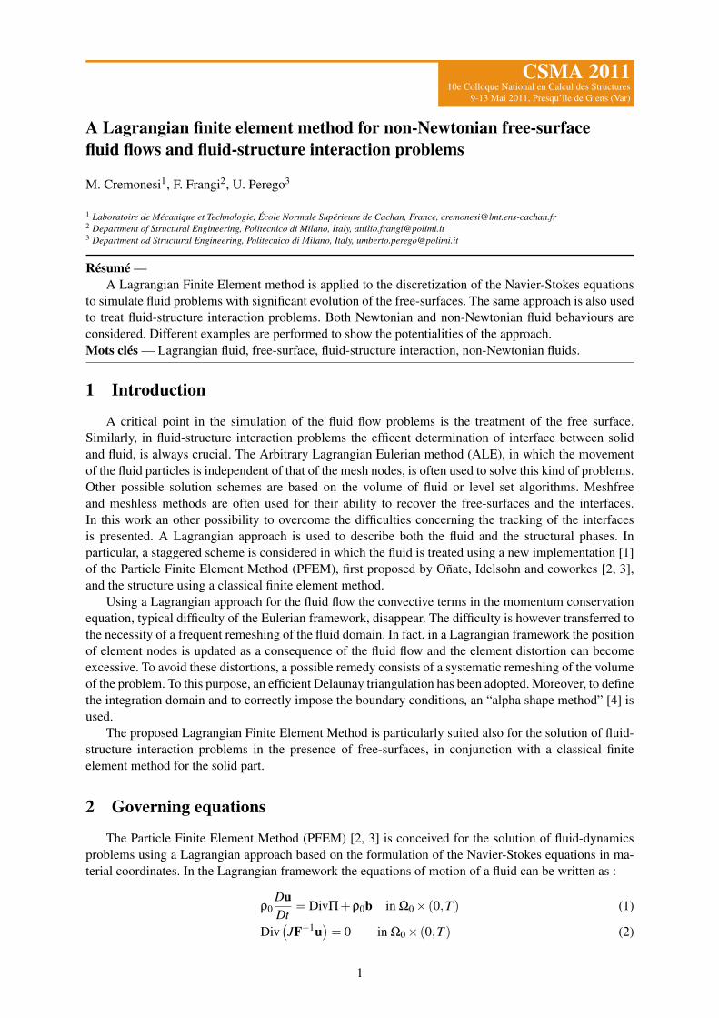
The PFEM, in the form implemented in the present work, consists of the following conceptual steps(see also [2] and reference therein). Figure 1 shows a pictorial representation of the steps.

1. Fill the fluid domain with a set of points referred to as "particles" (Figure 1(a)). The accuracy ofthe numerical solution is clearly dependent on the considered number of particles.

2. Generate a finite element mesh using the particles as nodes. This is achieved using a Delaunaytriangulation (Figure 1(b)).

3. Identify the external and internal boundaries to compute the domain integrals and to impose cor-rectly the boundary conditions (Figure 1(c)).

4. Solve the non-linear Lagrangian equations of motion (10)-(11) finding velocity and pressure atevery node of the mesh.

5. Update the particle positions using the computed values of velocity and pressure (Figure 1(d)).

6. Check the mesh distortion :– if the mesh is too distorted go back to step 2 and repeat for the next time step.– if the mesh is not too distorted go back to step 3 and repeat for the next time step.

3.1 Mesh generation and identification of external boundaries

To solve the Lagrangian Navier-Stokes equations in a domain defined by the particles, a finite elementmesh is necessary. A possibility to generate a mesh starting from a particle distribution is the Delaunaytriangulation. The Delaunay triangulation generates the convex hull of the set of particles, i.e. the convexfigure with minimum area that encloses all the particles belonging to the set.

3

(a) Initial point set (b) Mesh generation

(c) Boundary identification (d) Update of the particle position

FIGURE 1 – Steps of Particle Finite Element Method

Therefore, in a Lagrangian framework the external boundary Γt = ∂Ωt and the current volume Ωt

are defined by the position of the material particles. Every time that the mesh is regenerated with theDelaunay triangulation, the particles belonging to the boundary may change and the new boundary nodes(and therefore the particles) have to be identified. The identification process is divided in two phases :

– identification of the real shape of the particle distribution ;– identification of the nodes that belong to the boundary.

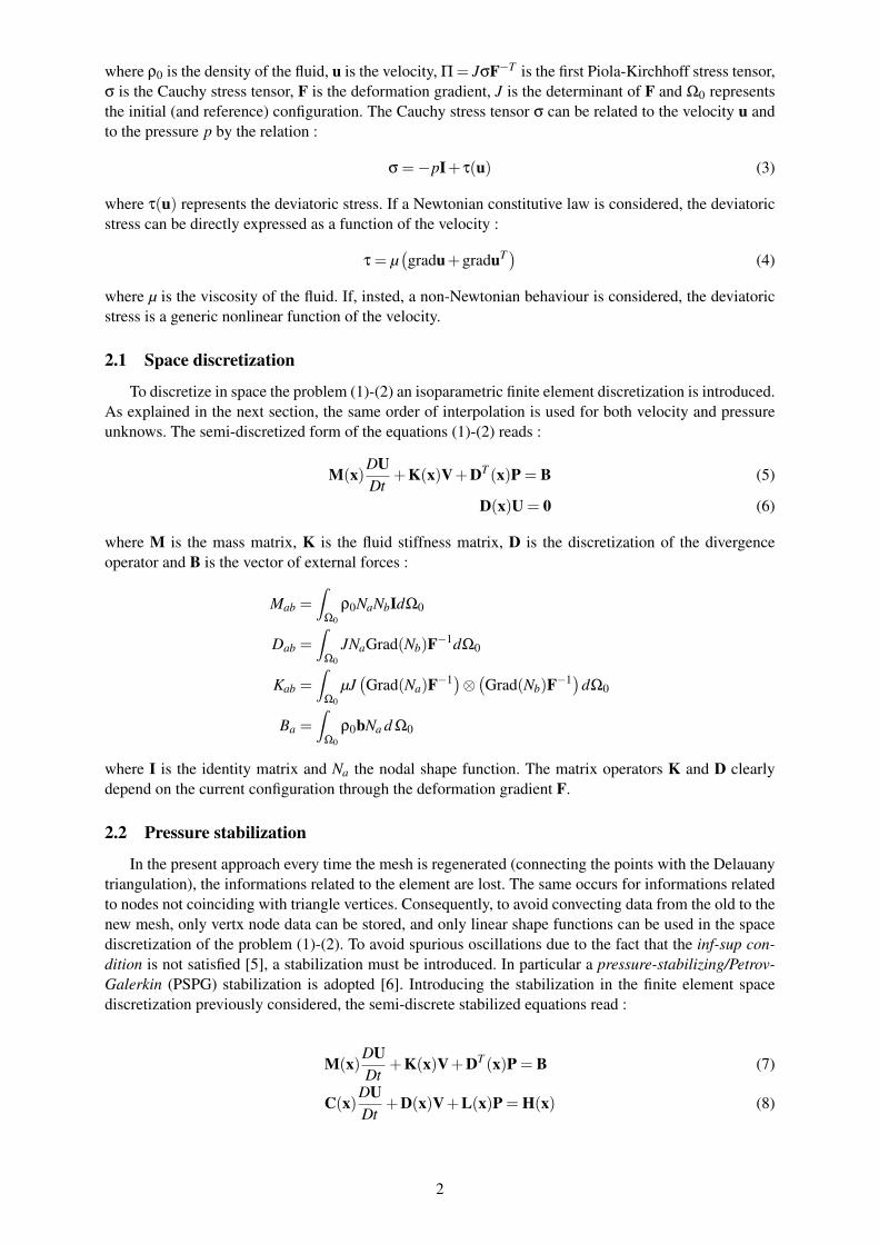
The second phase is almost trivial, but the first one is critical. As introduced, the Delaunay triangulationgenerates the convex hull of the set of particles. However, the convex hull may be not conformal withthe external boundaries. To clarify this problem, a set of points is shown in Figure 2(a) and its Delaunaytriangulation in Figure 2(b). It is clear that the Delaunay triangulation does not match the real boundaries.

(a) (b) (c)

FIGURE 2 – (a) Distrubution of points, (b) Delaunay triangulation, (c) Delaunay triangulation with α-shape.

A possibility to overcome this problem is to correct the generated mesh using the so called α-shapemethod [4] as proposed in [7]. The key idea is to remove the unnecessary triangles from the mesh using a

4

criterion based on the mesh distortion. For each triangle e of the mesh, the minimal distance he betweentwo nodes in the element and the radius Re of the circumcircle of the element are defined. If h is computedas the mean value of all the he, the shape factor :

αe =Re

h≥ 1√

3, (12)

is an index of the element distortion. It is worth recalling that Re/he = 1/√

3 is the ratio for an equilateraltriangle. All the elements that do not satisfy the condition :

αe ≤ α (13)

are removed from the mesh, where α ≥ 1 is assumed. Figure 2(c) shows the Delaunay triangulationcoupled with the alpha-shape scheme for the example introduced before.

In general, increasing the value of α, fewer triangles are removed from the original mesh and, forα→ ∞, the original Delaunay triangulation is always recovered.

Once the unnecessary triangles are removed from the Delaunay triangulation, the particles whichactually belong to the boundary can be identified.

The α-shape method can also be used for the identification of the fluid particles which separates fromthe rest of the domain. When a particle on the boundary is a vertex of only one triangle and the triangleis overly distorted, the particle is separated from the domain and all the mass of the triangle is assignedto this particle in order to preserve the total fluid mass. After separation, the motion of these particles isgoverned by the body force and the initial velocity which they are subjected to. At each new Delaunaytriangulation, the separated particles become vertices of triangles. In the case that a separated particle hasapproached enough the fluid free boundary, the triangle is not eliminated by the α-shape method checkand the particle is again incorporated in the fluid mass.

4 Fluid-structure interaction

The proposed Lagrangian Finite Element Method is particularly suited for the solution of fluid-structure interaction problems in the presence of free-surfaces, in conjunction with a classical finite ele-ment method for the solid part. A critical issue of fluid-structure interaction schemes is the identificationof the contact interfaces between the solid and fluid domains. The evolution of the interaction surfaces istracked using a novel algorithm which exploits the features of the Lagrangian approach based on the con-tinuous remeshing introduced for the fluid solution. The proposed algorithm is based on the superpositionof a set of fictitious fluid particles (called “ghost particles”) to the nodes of the solid domain, which cancome in contact with the fluid domain. When the Delaunay triangulation is performed, the alpha-shapecriterion selects those parts of the interface where the fluid particles can possibly come into contact withthe structure. If the two discretized domains are not in contact, the fluid and the solid analyses are per-formed separately without any interaction. If instead parts of the two discretized domains are in contact,a coupled analysis is performed with a Dirichlet-Neumann iterative approach. The fundamental steps ofthe interaction can be listed as follows.

– Superpose a set of ghost particles to the solid surfaces which can possibly come into contact withthe fluid domain.

– Perform the Delaunay triangulation.– Apply the α-shape method to remove the unnecessary triangles.– Check whether the fluid is in contact with the solid part. The fluid element is assumed to be in

contact with the solid if at least one of its nodes is a ghost particle.– If the two discretized domains are not in contact, the fluid and the solid analyses are performed

separately without any interaction.– If the two discretized domains are in contact, a coupled analysis is necessary.

5 Applications

The proposed scheme has been applied to both Newtonian and non-Newtonian fluids. Comparisonswith numerical benchmarks and with experimental results are presented to show its potentialities.

5

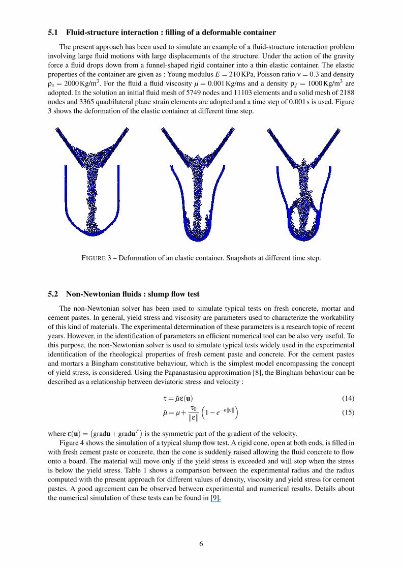
5.1 Fluid-structure interaction : filling of a deformable container

The present approach has been used to simulate an example of a fluid-structure interaction probleminvolving large fluid motions with large displacements of the structure. Under the action of the gravityforce a fluid drops down from a funnel-shaped rigid container into a thin elastic container. The elasticproperties of the container are given as : Young modulus E = 210KPa, Poisson ratio ν = 0.3 and densityρs = 2000Kg/m3. For the fluid a fluid viscosity µ = 0.001Kg/ms and a density ρ f = 1000Kg/m3 areadopted. In the solution an initial fluid mesh of 5749 nodes and 11103 elements and a solid mesh of 2188nodes and 3365 quadrilateral plane strain elements are adopted and a time step of 0.001s is used. Figure3 shows the deformation of the elastic container at different time step.

FIGURE 3 – Deformation of an elastic container. Snapshots at different time step.

5.2 Non-Newtonian fluids : slump flow test

The non-Newtonian solver has been used to simulate typical tests on fresh concrete, mortar andcement pastes. In general, yield stress and viscosity are parameters used to characterize the workabilityof this kind of materials. The experimental determination of these parameters is a research topic of recentyears. However, in the identification of parameters an efficient numerical tool can be also very useful. Tothis purpose, the non-Newtonian solver is used to simulate typical tests widely used in the experimentalidentification of the rheological properties of fresh cement paste and concrete. For the cement pastesand mortars a Bingham constitutive behaviour, which is the simplest model encompassing the conceptof yield stress, is considered. Using the Papanastasiou approximation [8], the Bingham behaviour can bedescribed as a relationship between deviatoric stress and velocity :

τ = µε(u) (14)

µ = µ+τ0

‖ε‖

(1− e−n‖ε‖

)(15)

where ε(u) =(gradu+graduT

)is the symmetric part of the gradient of the velocity.

Figure 4 shows the simulation of a typical slump flow test. A rigid cone, open at both ends, is filled inwith fresh cement paste or concrete, then the cone is suddenly raised allowing the fluid concrete to flowonto a board. The material will move only if the yield stress is exceeded and will stop when the stressis below the yield stress. Table 1 shows a comparison between the experimental radius and the radiuscomputed with the present approach for different values of density, viscosity and yield stress for cementpastes. A good agreement can be observed between experimental and numerical results. Details aboutthe numerical simulation of these tests can be found in [9].

6

FIGURE 4 – Mini-slump-flow test. Snapshots at different time steps for a cement paste.

density (Kg/m3) viscosity (Pa s) yield stress (Pa) exp. radius (m) computed radius (m)2252 4.018 18.0182 0.2249 0.22002242 3.511 7.4457 0.2668 0.25202231 3.009 2.4997 0.3333 0.32262252 5.014 25.8860 0.2249 0.22282242 3.836 10.6969 0.2682 0.28042231 3.585 3.5913 0.3333 0.3291

TABLE 1 – Mini-slump-flow test : comparisons for varying density, viscosity and yield stress for cementpastes.

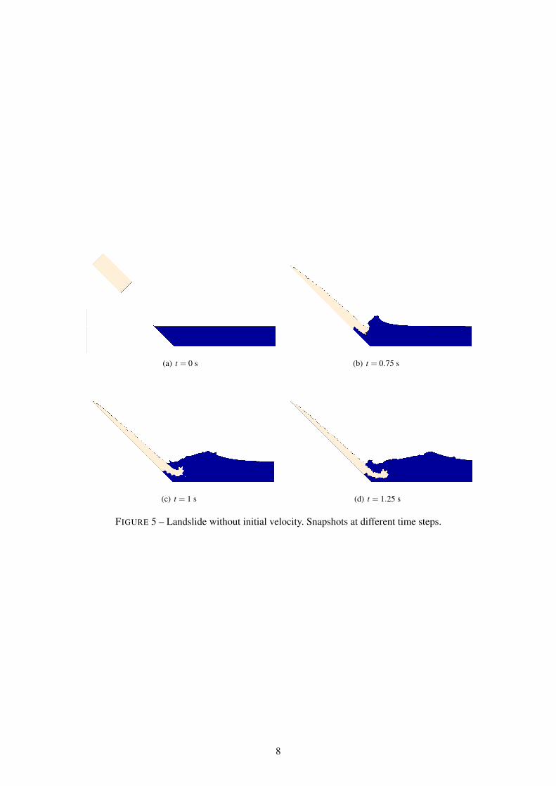
5.3 Deformable landslide simulation

The proposed approach is then used to simulate the wave generated by a deformable mass of granularmaterial sliding in a water channel. This example is particularly interesting because impulse waves inbays, lakes or reservoirs generated by landslides or rock falls may propagate with possibly catastrophicconsequences for the surronding enviroment.

For the numerical simulation of the sliding mass a non-Newtonian Bingham fluid behaviour is as-sumed, while a classical Newtonian behaviour is considered for the water [10]. Figure 5 shows snapshotsof the analysis at different time steps.

Références

[1] M. Cremonesi, A. Frangi, and U. Perego. A lagrangian finite element approach for the analysisof fuid-structure interaction problems. International Journal for Numerical Methods in Engineering,(doi :10.1002/nme.2911), 2010.

[2] E. Oñate, S.R. Idelsohn, F. Del Pin, and R. Aubry. The particle finite element method. An overview. Inter-national Journal of Computational Methods, 1(2) :267–307, 2004.

[3] S.R. Idelsohn, E. Oñate, and F. Del Pin. The particle finite element method : a powerful tool to solve in-compressible flows with free-surfaces and breaking waves. International Journal for Numerical Methods inEngineering, 61(7) :964–989, 2004.

[4] H. Edelsbrunner and E. P. Mucke. Three dimensional alpha shapes. ACM Transactions on Graphics,13(1) :43–72, January 1994.

[5] F. Brezzi and M. Fortin. Mixed and Hybrid Finite Element Method. Springer-Veralg, 1991.[6] T. E. Tezduyar, S. Mittal, S. E. Ray, and R. Shih. Incompressible flow computations with stabilized bilinear

and linear equal-order-interpolation velocity-pressure elements. Computer Methods in Applied Mechanicsand Engineering, 95(2) :221–242, March 1992.

[7] S. R. Idelsohn, E. Oñate, and F. Del Pin. A lagrangian meshless finite element method applied to fluid-structure interaction problems. Computers & Structures, 81(8-11) :655–671, May 2003.

[8] T. C. Papanastasiou. Flows of materials with yield. Journal of Rheology, 31(5) :385–404, 1987.[9] M. Cremonesi, L. Ferrara, A. Frangi, and U. Perego. Simulation of the flow of fresh cementitious suspensions

by a lagrangian finite element approach,. Journal of Non-Newtonian Fluid Mechanics, 165 :1555–1563, 2010.[10] M. Cremonesi, A. Frangi, and U. Perego. A lagrangian finite element approach for the simulation of water-

waves induced by landslides,. Computers and Structures, doi :10.1016/j.compstruc.2010.12.005, 2011.

7

(a) t = 0 s (b) t = 0.75 s

(c) t = 1 s (d) t = 1.25 s

FIGURE 5 – Landslide without initial velocity. Snapshots at different time steps.

8