A KAM theorem without action-angle variables for elliptic lower dimensional tori
64
A KAM theorem without action-angle variables for elliptic lower dimensional tori Alejandro Luque Jordi Villanueva February 15, 2010 Departament de Matem` atica Aplicada I, Universitat Polit` ecnica de Catalunya, Diagonal 647, 08028 Barcelona (Spain). [email protected] [email protected] Abstract We study elliptic lower dimensional invariant tori of Hamiltonian systems via parame- terizations. The method is based in solving iteratively the functional equations that stand for invariance and reducibility. In contrast with classical methods, we do not assume that the system is close to integrable nor that is written in action-angle variables. We only re- quire an approximation of an invariant torus of fixed vector of basic frequencies and a basis along the torus that approximately reduces the normal variational equations to constant co- efficients. We want to highlight that this approach presents many advantages compared with methods which are built in terms of canonical transformations, e.g., it produces sim- pler and more constructive proofs that lead to more efficient numerical algorithms for the computation of these objects. Such numerical algorithms are suitable to be adapted in order to perform computer assisted proofs. Mathematics Subject Classification: 37J40 Keywords: Elliptic invariant tori; KAM theory; Parameterization methods
-
Upload
independent -
Category
Documents
-
view
0 -
download
0
Transcript of A KAM theorem without action-angle variables for elliptic lower dimensional tori
A KAM theorem without action-angle variables forelliptic lower dimensional tori
Alejandro Luque Jordi Villanueva
February 15, 2010
Departament de Matematica Aplicada I,Universitat Politecnica de Catalunya,
Diagonal 647, 08028 Barcelona (Spain)[email protected] [email protected]
Abstract
We study elliptic lower dimensional invariant tori of Hamiltonian systems via parame-terizations. The method is based in solving iteratively the functional equationsthat standfor invariance and reducibility. In contrast with classical methods, we do not assume thatthe system is close to integrable nor that is written in action-angle variables. Weonly re-quire an approximation of an invariant torus of fixed vector of basic frequencies and a basisalong the torus that approximately reduces the normal variational equationsto constant co-efficients. We want to highlight that this approach presents many advantages comparedwith methods which are built in terms of canonical transformations, e.g., it produces sim-pler and more constructive proofs that lead to more efficient numerical algorithms for thecomputation of these objects. Such numerical algorithms are suitable to be adapted in orderto perform computer assisted proofs.
Mathematics Subject Classification: 37J40Keywords: Elliptic invariant tori; KAM theory; Parameterization methods
2 KAM theorem without action-angle for elliptic tori
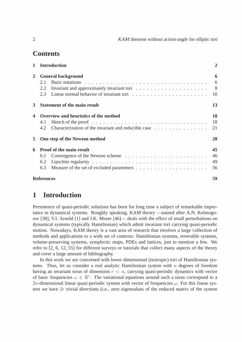
Contents
1 Introduction 2
2 General background 62.1 Basic notations . . . . . . . . . . . . . . . . . . . . . . . . . . . . . . . . . . 62.2 Invariant and approximately invariant tori . . . . . . . . . .. . . . . . . . . . 82.3 Linear normal behavior of invariant tori . . . . . . . . . . . . .. . . . . . . . 10
3 Statement of the main result 13
4 Overview and heuristics of the method 184.1 Sketch of the proof . . . . . . . . . . . . . . . . . . . . . . . . . . . . . . . .184.2 Characterization of the invariant and reducible case . . .. . . . . . . . . . . . 21
5 One step of the Newton method 28
6 Proof of the main result 456.1 Convergence of the Newton scheme . . . . . . . . . . . . . . . . . . . . .. . 466.2 Lipschitz regularity . . . . . . . . . . . . . . . . . . . . . . . . . . . . .. . . 496.3 Measure of the set of excluded parameters . . . . . . . . . . . . .. . . . . . . 56
References 59
1 Introduction
Persistence of quasi-periodic solutions has been for long time a subject of remarkable impor-tance in dynamical systems. Roughly speaking, KAM theory —named after A.N. Kolmogo-rov [38], V.I. Arnold [1] and J.K. Moser [46]— deals with the effect of small perturbations ondynamical systems (typically Hamiltonian) which admit invariant tori carrying quasi-periodicmotion. Nowadays, KAM theory is a vast area of research that involves a large collection ofmethods and applications to a wide set of contexts: Hamiltonian systems, reversible systems,volume-preserving systems, symplectic maps, PDEs and lattices, just to mention a few. Werefer to [2, 6, 12, 55] for different surveys or tutorials that collect many aspects of the theoryand cover a large amount of bibliography.
In this work we are concerned with lower dimensional (isotropic) tori of Hamiltonian sys-tems. Thus, let us consider a real analytic Hamiltonian system with n degrees of freedomhaving an invariant torus of dimensionr < n, carrying quasi-periodic dynamics with vectorof basic frequenciesω ∈ R
r. The variational equations around such a torus correspond to a2n-dimensional linear quasi-periodic system with vector of frequenciesω. For this linear sys-tem we have2r trivial directions (i.e., zero eigenvalues of the reduced matrix of the system
A. Luque and J.Villanueva 3
restricted to these directions) associated to the tangent directions of the torus and the symplec-tic conjugate ones (these trivial directions are usually referred as the central directions of thetorus). If the remaining2(n − r) directions (normal directions of the torus) are hyperbolic, wesay that the torus is hyperbolic or whiskered. Hyperbolic tori are very robust under perturba-tions [15, 20, 23, 28, 41]. For example, if we consider a perturbation of the system dependinganalytically on external parameters, it can be established, under suitable conditions, the exis-tence of an analytic (with respect to these parameters) family of hyperbolic tori having the samebasic frequencies. In the above setting, if the torus possesses some elliptic (oscillatory) normaldirections we say that it is elliptic or partially elliptic.In this case the situation is completely dif-ferent, since we have to take into account combinations between basic and normal frequencies inthe small divisors that appear in the construction of these tori (the corresponding non-resonanceconditions are usually referred as Melnikov conditions [43, 44]). As a consequence, families ofelliptic or partially elliptic invariant tori with fixed basic frequenciesω cannot be continuous ingeneral, but they turn out to be Cantorian with respect to parameters. First rigorous proofs ofexistence of elliptic tori were given in [49] forr = n − 1 and in [17, 40] forr < n. We referalso to [5, 6, 24, 31, 35, 36, 52, 54, 62, 64, 66] as interestingcontributions covering differentpoints of view.
The main source of difficulty in presence of elliptic normal directions is the so-called lack ofparameters problem [6, 49, 63]. Basically, since we have onlyas many internal parameters (“ac-tions”) as the number of basic frequencies of the torus, we cannot control simultaneously thenormal ones, so we cannot prevent them from “falling into resonance”. This is equivalent to saythat, for a given Hamiltonian system, we cannot construct a torus with a fixed set of basic andnormal frequencies because there are not enough parameters. The previous fact leads to the ex-clusion of a small set of these internal parameters in order to avoid resonances involving normalfrequencies. To control the measure of the set of excluded parameters, it is necessary to assumethat the normal frequencies “move” as a function of the internal parameters. Another possibilityto overcome this problem is to apply the so-called Broer-Huitema-Takens theory (see [7]). Thisconsists in adding as many (external) parameters as needed to control simultaneously the valuesof both basic and normal frequencies (this process is referred as unfolding). With this setting, wecan prove that —under small perturbations— there exist invariant tori for a nearly full-measureCantor set of parameters. TheC∞-Whitney smoothness of this construction is also established.Finally, in order to ensure the existence of invariant tori for the original system (free of pa-rameters), one can apply the so-called Herman’s method. Indeed, external parameters can beeliminated —under very weak non-degeneracy conditions— bymeans of an appropriate techni-cal result concerning Diophantine approximation on submanifolds (see [6, 59, 61, 62, 63, 64]).
Another issue linked to persistence of lower dimensional invariant tori refers to reducibilityof the normal variational equations (at least in the elliptic directions) which is usually askedin order to simplify the study of the linearized equations involved. In order to achieve thisreducibility, it is typical to consider second order Melnikov conditions [43, 44] to control thesmall divisors of the cohomological equations appearing inthe construction of the reduced ma-
4 KAM theorem without action-angle for elliptic tori
trix. Other approaches for studying persistence of invariant tori in the elliptic context, withoutsecond order Melnikov conditions, are discussed in Remark 3.10.
Classical methods for studying persistence of lower dimensional tori are based on canonicaltransformations performed on the Hamiltonian function. These methods typically deal with aperturbative setting in such a way that the problem is written as a perturbation of an “integrable”Hamiltonian (in the sense that it has a continuous family of reducible invariant tori), and takeadvantage of the existence of action-angle-like coordinates for the unperturbed Hamiltonian sys-tem. These coordinates play an important role in solving thecohomological equations involvedin the iterative KAM process, and they also allow us to control the isotropic1 character of thetori thus simplifying a lot of details. However, classical approaches present some shortcomings,mainly due to the fact that they only allow us to face perturbative problems. For example:
• In many practical applications (design of space missions [21, 22], study of models inCelestial Mechanics [11], Molecular Dynamics [53, 65] or Plasma-Beam Physics [45],just to mention a few) we have to consider non-perturbative systems. For such systems wecan obtain approximate invariant tori by means of numericalcomputations or asymptoticexpansions, but in general we cannot apply classical results to prove the existence of theseobjects. Furthermore, in some cases it is possible to identify an integrable approximationof a given system but the remaining part cannot be consideredas an arbitrarily smallperturbation.
• Even if we are studying a concrete perturbative problem, sometimes it is very compli-cated to establish action-angle variables for the unperturbed Hamiltonian. In some casesaction-angle variables are not explicit, become singular or introduce problems of regu-larity (for example, when we approach to a separatrix). Although in many contexts thisshortcoming has been solved by means of several techniques (see for example [16, 27, 51]for a construction in the case of an integrable Hamiltonian or [8, 37] for a constructionaround a particular object), it introduces more technical difficulties in the problem.
• From the computational viewpoint, methods based on transformations are sometimes in-efficient and quite expensive. This is a serious difficulty inorder to implement numericalmethods or computer assisted proofs based on them.
An alternative to the classical approach is the use of so-called parameterization methods,which consist in performing an iterative scheme to solve theinvariance equation of the torus.Instead of performing canonical transformations, this scheme is carried out by adding a smallfunction to the previous approximation of the torus. This function is obtained by solving (ap-proximately) the linearized equation around the approximated torus (Newton method). Suchapproach is suitable for studying existence of invariant tori of Hamiltonian systems without us-ing neither action-angle variables nor a perturbative setting. We point out that the geometry of
1If we pull-back an isotropic torus by means of a symplectomorphism, the isotropic character is preserved.
A. Luque and J.Villanueva 5
the problem plays an important role in the study of these equations. Such geometric approach—also referred as KAM theory without action-angle variables— was introduced in [13] for La-grangian tori and extended in [20] to hyperbolic lower dimensional tori, following long-timedeveloped ideas (relevant work can be found in [11, 31, 47, 48, 58, 60, 67]). Roughly speaking,the insight of these methods is summarized in the following quote from [31]:“...near approxi-mate solutions of certain equations satisfying certain non-degeneracy assumptions, we can findtrue solutions defined on a large set.”
The aim of this paper is to adapt parameterization methods tostudy normally elliptic toriwithout using action-angle variables and in a non-perturbative setting. Concretely, we assumethat we have a 1-parameter family of Hamiltonian systems forwhich we know a 1-parameterfamily of approximately invariant lower dimensional elliptic tori —all of them with the samevector of basic frequencies— and also approximations of thevectors of normal frequencies andthe corresponding normal directions associated to these frequencies (i.e., a basis of the nor-mal directions along each torus that approximately reducesthe normal variational equationsto constant coefficients). Then, we show that under suitablehypotheses of non-resonance andnon-degeneracy, for a Cantorian subset of parameters —of large relative Lebesgue measure—there exists a true elliptic torus close to the approximate one, having the same vector of basicfrequencies and slightly modified vector of normal frequencies. The scheme to deal with re-ducibility of the normal directions of these tori is the maincontribution of this paper, and itconsists in performing suitable (small) corrections in thenormal directions at each step of theiterative procedure.
This setting has been selected in order to simplify some technical aspects of the result —bothin the assumptions and in the proof— thus highlighting the geometric construction of the paper.We point out that all the basic ideas linked to parameterization methods, without using action-angle variables, for reducible lower-dimensional tori arepresent in our approach. In Section 3we discuss several extensions and generalizations that canbe tackled with the method presentedin this paper.
Let us remark that parameterization methods, as presented above, are computationally ori-ented in the sense that they can be implemented numerically,thus obtaining very efficient algo-rithms for the computation of invariant tori. For example, if we approximate a torus by usingNFourier modes, such algorithms allow us to compute the object with a cost of orderO(N log N)in time andO(N) in memory (see Remark 3.11). This is another advantage of our approach incontrast with classical methods based on transformation theory. The reader interested in suchalgorithms is referred to [14] for the implementation of theideas in [13, 20] for Lagrangianand whiskered tori (see also [9] for the case of lattices and twist maps) and to [32] for the im-plementation of the ideas of [34] for reducible elliptic andhyperbolic tori for quasi-periodicskew-product maps (in this case, which corresponds to quasi-periodic perturbations of equilib-rium points for flows, the geometric part discussed in the present paper is not required).
Finally, we observe that in presence of hyperbolic directions one can approach the prob-lem by combining techniques in [20] (for studying hyperbolic directions) together with those
6 KAM theorem without action-angle for elliptic tori
introduced here (for studying elliptic directions). Indeed, the methodology presented in thiswork can be adapted to deal with invariant tori with reducible hyperbolic directions, but thisassumption is quite restrictive (see [25]) in the hyperbolic context (reducibility is not requiredin [20]).
The paper is organized as follows. In Section 2 we provide some notations, definitionsand background of the problem. In Section 3 we state the main result of this paper and wediscuss several extensions and generalizations of the method presented. A motivating sketchof the construction performed in the proof of this result is given in Section 4, together with adetailed description of some geometric properties of elliptic lower dimensional invariant toriof Hamiltonian systems. Next, in Section 5 we perform one step of the iterative method tocorrect both an approximation of an elliptic invariant torus and a basis along this torus thatapproximately reduces the normal variational equations toconstant coefficients. The new errorsin invariance and reducibility are quadratic in terms of theprevious ones. The main result isproved in Section 6.
2 General background
In this section we introduce some notation and, in order to help the reader, we recall the basicterminology and concepts related to the problem. Thus, after setting the notation used along thepaper in Section 2.1, we provide the basic definitions regarding lower dimensional invariant toriof Hamiltonian systems (Section 2.2) and their normal behavior (Section 2.3).
2.1 Basic notations
Given a real or complex functionf of several variables, we denoteDf the Jacobian matrix,grad f = Df⊤ the gradient vector andhess f = D2f the Hessian matrix, respectively.
For any complex numberz ∈ C we denotez∗ ∈ C its complex conjugate number andRe(z), Im(z) the real and imaginary parts ofz, respectively. We extend these notations tocomplex vectors and matrices.
Given a complex vectorv ∈ Cl we denote bydiag (v) ∈ Ml×l(C) the diagonal matrix
having the components ofv in the diagonal. Moreover, givenZ ∈ Ml×l(C), we denote bydiag (Z) ∈ Ml×l(C) the diagonal matrix having the same diagonal entries asZ.
For anyk ∈ Zr, we denote|k|1 = |k1| + . . . + |kr|. Given a vectorx ∈ C
l, we set|x| = supj=1,...,l |xj| for the supremum norm and we extend the notation to the induced normfor complex matrices. Furthermore, given an analytic function f , with bounded derivatives in acomplex domainU ⊂ C
l, andm ∈ N we introduce theCm-norm forf as
‖f‖Cm,U = supk∈(N∪0)l
0≤|k|1≤m
supz∈U
|Dkf(z)|.
A. Luque and J.Villanueva 7
We denote byTr = Rr/(2πZ)r the realr-dimensional torus, withr ≥ 1. We use the
| · |-norm introduced above to define the complex strip aroundTr of width ρ > 0 as
∆(ρ) = θ ∈ Cr/(2πZ)r : |Im(θ)| ≤ ρ.
Accordingly we will consider the Banach space of analytic functionsf : ∆(ρ) → C equippedwith the norm
‖f‖ρ = supθ∈∆(ρ)
|f(θ)|.
Similarly, if f takes values inCl, we set‖f‖ρ = |(‖f1‖ρ, . . . , ‖fl‖ρ)|. If f is a matrix valuedfunction, we extend‖f‖ρ by computing the| · |-norm of the constant matrix defined by the‖·‖ρ-norms of the entries off . We observe that if the matrix product is defined then this space is aBanach algebra and we have‖f1f2‖ρ ≤ ‖f1‖ρ‖f2‖ρ. In addition, we can use Cauchy estimates
∥∥∥∥∂f
∂θj
∥∥∥∥ρ−δ
≤‖f‖ρ
δ, j = 1, . . . , r.
For any functionf analytic onTr and taking values inC, C
l or in a space of complexmatrices, we denote its Fourier series as
f(θ) =∑
k∈Zn
fkei〈k,θ〉, fk =
1
(2π)r
∫
Tr
f(θ)e−i〈k,θ〉dθ
and its average as[f ]Tr = f0. We also setf(θ) = f(θ)−[f ]
Tr . Moreover, we have the followingbounds
| [f ]Tr | ≤ ‖f‖ρ, ‖f‖ρ ≤ 2‖f‖ρ, |fk| ≤ ‖f‖ρe
−ρ|k|1 .
Now, we introduce some notation regarding Lipschitz regularity. Assume thatf(µ) is afunction defined forµ ∈ I ⊂ R —the subsetI may not be an interval— taking values inC, C
l
or Ml1×l2(C). We say thatf is Lipschitz with respect toµ on the setI if
LipI(f) = supµ1,µ2∈Iµ1 6=µ2
|f(µ2) − f(µ1)|
|µ2 − µ1|< ∞.
The valueLipI(f) is called the Lipschitz constant off on I. For these functions we define‖f‖I = supµ∈I |f(µ)|. Similarly, if we have a familyµ ∈ I ⊂ R 7→ fµ, wherefµ is a functiononT
r taking values inC, Cl or Ml1×l2(C), we extend the previous notations as
LipI,ρ(f) = supµ1,µ2∈Iµ1 6=µ2
‖fµ2 − fµ1‖ρ
|µ2 − µ1|< ∞, ‖f‖I,ρ = sup
µ∈I‖fµ‖ρ.
8 KAM theorem without action-angle for elliptic tori
Analogously, given a familyµ ∈ I ⊂ R 7→ fµ, wherefµ is an analytic function with boundedderivatives in a complex domainU ⊂ C
l, we introduce form ∈ N
LipI,Cm,U(f) = supµ1,µ2∈Iµ1 6=µ2
‖fµ1 − fµ2‖Cm,U
|µ1 − µ2|, ‖f‖I,Cm,U = sup
µ∈I‖fµ‖Cm,U .
Finally, we say thatf is Lipschitz from below with respect toµ on the setI if
lipI(f) = infµ1,µ2∈Iµ1 6=µ2
|f(µ2) − f(µ1)|
|µ2 − µ1|< ∞.
In this work we are concerned with Hamiltonian systems inR2n with respect to the standard
symplectic formΩ0, given byΩ0(ξ, η) = ξ⊤Jnη where
Jn =
(0 Idn
−Idn 0
)
is the canonical skew-symmetric matrix. We extend the notation above to writeJj for any1 ≤ j ≤ n, andIdj for any1 ≤ j ≤ 2n. For the sake of simplicity, we denoteJ = Jn andId = Id2n.
Finally, given matrix-valued functionsA : Tr → M2n×la(C) andB : T
r → M2n×lb(C),we set the notationsGA,B(θ) = A(θ)⊤B(θ), ΩA,B(θ) = A(θ)⊤JB(θ), GA(θ) = GA,A(θ) andΩA(θ) = ΩA,A(θ).
2.2 Invariant and approximately invariant tori
Given a Hamiltonian functionh : U ⊂ R2n → R, we study the existence of lower dimensional
quasi-periodic invariant tori for the Hamiltonian vector fieldXh(x) = Jgrad h(x).
Definition 2.1. For any integer1 ≤ r ≤ n, T ⊂ U is an r-dimensional quasi-periodicinvariant torus with basic frequenciesω ∈ R
r for Xh, if T is invariant under the flow ofXh
and there exists a parameterization given by an embeddingτ : Tr → U such thatT = τ(Tr),
making the following diagram commute
Tr
Tr
T T
-Tt,ω
?
τ
?
τ
-φt|T
(1)
whereTt,ω(x) = x + ωt is the (parallel) flow of the constant vector field
Lω = ω1∂
∂θ1
+ . . . + ωr∂
∂θr
A. Luque and J.Villanueva 9
andφt is the flow of the Hamiltonian vector fieldXh. In addition, if
〈k, ω〉 6= 0, ∀k ∈ Zr\0, (2)
then we say thatω is non-resonant.
If ω ∈ Rr is non-resonant, then the quasi-periodic functionz(t) = τ(ωt + θ0) is an integral
curve ofXh for anyθ0 ∈ Tn that fills denselyT . Equivalently, we have that the embeddingτ
satisfies
Lωτ(θ) = Xh(τ(θ)). (3)
By means ofτ we can pull-back toTr both the restrictions toT of the standard metric andthe symplectic structure, obtaining the following matrix representations
GDτ (θ) = Dτ(θ)⊤Dτ(θ), ΩDτ (θ) = Dτ(θ)⊤JDτ(θ), θ ∈ Tr.
Remark 2.2. We note that asτ is an embedding we haverank(Dτ(θ)) = r for everyθ ∈ Tr, so
it turns out thatdet GDτ (θ) 6= 0 for everyθ ∈ Tr. Moreover, we see that the average[ΩDτ ]Tr
is zero since if we writeτ(θ) = (x(θ), y(θ)) then we haveΩDτ (θ) = Dα(θ) − Dα(θ)⊤, whereα(θ) = Dx(θ)⊤y(θ) and, by definition,[Dα]
Tr = 0.
Lemma 2.3. Let h : U ⊂ R2n → R be a Hamiltonian function andT an r-dimensional
invariant torus forXh of non-resonant frequenciesω. Then the submanifoldT is isotropic, i.e.,ΩDτ (θ) = 0 for everyθ ∈ T
r. In particular, if r = n thenT is Lagrangian.
Remark 2.4. Along the text there appear many functions depending onθ ∈ Tr. In order to
simplify the notation sometimes we omit the dependence onθ —eventually we even omit the factthat some functions are evaluated atτ(θ) if there is no source of confusion.
Proof of Lemma 2.3.The isotropic character ofT is obtained as it was done in [13]. First, wecompute
Lω(ΩDτ ) = Lω(Dτ⊤JDτ) = [D(Lωτ)]⊤JDτ + Dτ⊤JD(Lωτ)
= [Jhess h(τ)Dτ ]⊤JDτ + Dτ⊤JJhess h(τ)Dτ = 0,
where we used thatD Lω = Lω D, the hypothesisLωτ(θ) = Xh(τ(θ)) and the propertiesJ⊤ = −J andJ2 = −Id. Then, sinceω is non-resonant, the fact that the derivativeLω vanishesimplies thatΩDτ = [ΩDτ ]Tr . Finally, from Remark 2.2 we conclude thatΩDτ = 0.
Finally, we set the idea of parameterization of an approximately invariant torus. Essentially,we measure how far to commute is diagram (1).
10 KAM theorem without action-angle for elliptic tori
Definition 2.5. Given a Hamiltonianh : U ⊂ R2n → R and an integer1 ≤ r ≤ n, we say that
T ⊂ U is an r-dimensional approximately quasi-periodic invariant torus with non-resonantbasic frequenciesω ∈ R
r for Xh provided that there exists an embeddingτ : Tr → U , such
thatT = τ(Tr), satisfying
Lωτ(θ) = Jgrad h(τ(θ)) + e(θ),
wheree : Tr → R
2n is “small” in a suitable norm.
Among the conditions needed to find a true invariant torus around an approximately invari-ant one, we are concerned with Diophantine conditions on thevector of basic frequencies.
Definition 2.6. We say thatω ∈ Rr satisfies Diophantine conditions of(γ, ν)-type, forγ > 0
andν > r − 1, if
|〈k, ω〉| ≥γ
|k|ν1, k ∈ Z
r\0. (4)
It is well-known that if we consider a fixedν then, for almost everyω ∈ Rr, there isγ > 0
for which (4) is fulfilled (see [42]).
2.3 Linear normal behavior of invariant tori
In order to study the behavior of the solutions in a neighborhood of anr-dimensional quasi-periodic invariant torus of basic frequenciesω —parameterized byτ— it is usual to considerthe variational equations around the torus, given by
Lωξ(θ) = Jhess h(τ(θ))ξ(θ). (5)
If r = 1 the system (5) is2π/ω-periodic. Then, following Floquet’s theorem, there existsa linear periodic change of variables that reduces the system to constants coefficients. Ifr >1, then we consider reducibility to constant coefficients (inthe sense of Lyapunov-Perron) asfollows.
Definition 2.7. We say that the invariant torusT in Definition 2.1 is reducible if there existsa linear change of coordinatesξ = M(θ)η, defined forθ ∈ T
r, such that the variationalequations(5) turn out to beLωη(θ) = Bη(θ), whereB ∈ M2n×2n(C).
It is immediate to check that this property is equivalent to the fact thatM satisfies thedifferential equation
LωM(θ) = Jhess h(τ(θ))M(θ) − M(θ)B. (6)
In the Lagrangian caser = n, under regularity assumptions, such transformation existsprovidedω satisfies (4) due to the geometric constrains of the problem (see [13]). Indeed, wecan take derivatives at both sides of the invariance equation (3), thus obtaining
LωDτ(θ) = Jhess h(τ(θ))Dτ(θ).
A. Luque and J.Villanueva 11
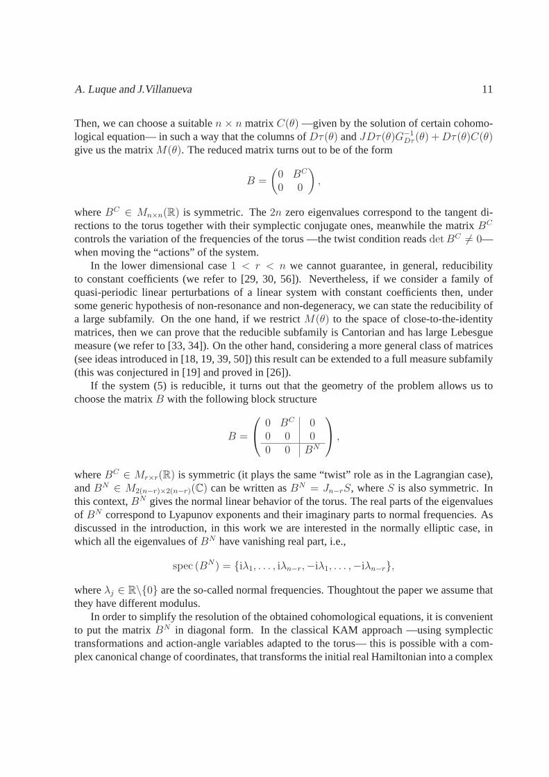
Then, we can choose a suitablen × n matrix C(θ) —given by the solution of certain cohomo-logical equation— in such a way that the columns ofDτ(θ) andJDτ(θ)G−1
Dτ (θ) + Dτ(θ)C(θ)give us the matrixM(θ). The reduced matrix turns out to be of the form
B =
(0 BC
0 0
),
whereBC ∈ Mn×n(R) is symmetric. The2n zero eigenvalues correspond to the tangent di-rections to the torus together with their symplectic conjugate ones, meanwhile the matrixBC
controls the variation of the frequencies of the torus —the twist condition readsdet BC 6= 0—when moving the “actions” of the system.
In the lower dimensional case1 < r < n we cannot guarantee, in general, reducibilityto constant coefficients (we refer to [29, 30, 56]). Nevertheless, if we consider a family ofquasi-periodic linear perturbations of a linear system with constant coefficients then, undersome generic hypothesis of non-resonance and non-degeneracy, we can state the reducibility ofa large subfamily. On the one hand, if we restrictM(θ) to the space of close-to-the-identitymatrices, then we can prove that the reducible subfamily is Cantorian and has large Lebesguemeasure (we refer to [33, 34]). On the other hand, considering a more general class of matrices(see ideas introduced in [18, 19, 39, 50]) this result can be extended to a full measure subfamily(this was conjectured in [19] and proved in [26]).
If the system (5) is reducible, it turns out that the geometryof the problem allows us tochoose the matrixB with the following block structure
B =
0 BC 00 0 00 0 BN
,
whereBC ∈ Mr×r(R) is symmetric (it plays the same “twist” role as in the Lagrangian case),andBN ∈ M2(n−r)×2(n−r)(C) can be written asBN = Jn−rS, whereS is also symmetric. Inthis context,BN gives the normal linear behavior of the torus. The real partsof the eigenvaluesof BN correspond to Lyapunov exponents and their imaginary partsto normal frequencies. Asdiscussed in the introduction, in this work we are interested in the normally elliptic case, inwhich all the eigenvalues ofBN have vanishing real part, i.e.,
spec (BN) = iλ1, . . . , iλn−r,−iλ1, . . . ,−iλn−r,
whereλj ∈ R\0 are the so-called normal frequencies. Thoughtout the paperwe assume thatthey have different modulus.
In order to simplify the resolution of the obtained cohomological equations, it is convenientto put the matrixBN in diagonal form. In the classical KAM approach —using symplectictransformations and action-angle variables adapted to thetorus— this is possible with a com-plex canonical change of coordinates, that transforms the initial real Hamiltonian into a complex
12 KAM theorem without action-angle for elliptic tori
one, having some symmetries. As these symmetries are preserved by the canonical transforma-tions performed along these classical proofs, the final Hamiltonian can be realified and thusthe obtained tori are real. In this paper we perform this complexification by selecting a com-plex matrix functionN : T
r → M2n×(n−r)(C) associated to the eigenfunctions of eigenvaluesiλ1, . . . , iλn−r. It is clear that the real and imaginary parts of these vectors span the associatedreal normal subspace at any point of the torus. Indeed, from Equation (6), the matrix functionN satisfies
LωN(θ) = Jhess h(τ(θ))N(θ) − N(θ)Λ,
whereΛ = diag (iλ) = diag (iλ1, . . . , iλn−r). Then, together with these vectors, we resort tothe use of the complex conjugate ones, that clearly satisfy
LωN∗(θ) = Jhess h(τ(θ))N∗(θ) + N∗(θ)Λ,
to span a basis of the complexified normal space along the torus (this is guaranteed by theconditionsdet GN,N∗ 6= 0 onT
r).As we have pointed out in the introduction of the paper, in order to face the resolution of
the cohomological equations standing for invariance and reducibility of elliptic tori, we assumeadditional non-resonance conditions apart from (2).
Definition 2.8. We say that the normal frequenciesλ ∈ Rn−r are non-resonant with respect to
ω ∈ R if〈k, ω〉 + λi 6= 0, ∀k ∈ Z
r, i = 1, . . . , n − r, (7)
and〈k, ω〉 + λi ± λj 6= 0, ∀k ∈ Z
r\0, i, j = 1, . . . , n − r. (8)
Conditions(7) and (8) are referred as first and second order Melnikov conditions, respectively(see [43, 44]).
In the spirit of Definition 2.5, we introduce the idea of approximate reducibility as follows.
Definition 2.9. We say that the approximately invariant torusT in Definition 2.5 is approxi-mately elliptic if there exists a mapN : T
r → M2n×(n−r)(C) and normal frequenciesλ ∈ Rn−r,
which are non-resonant with respect toω, satisfying
LωN(θ) = Jhess h(τ(θ))N(θ) − N(θ)Λ + R(θ),
whereΛ = diag (iλ), det GN,N∗ 6= 0 on Tr and R : T
r → M2n×(n−r)(C) is “small” in asuitable norm.
In order to avoid the effect of the small divisors associatedto (7) and (8), we assume addi-tional Diophantine conditions.
A. Luque and J.Villanueva 13
Definition 2.10. Let us consider non-resonant basic and normal frequencies(ω, λ) ∈ Rr×R
n−r
and constantsγ > 0 andν > r−1. We say thatλ satisfies Diophantine conditions of(γ, ν)-typewith respect toω if
|〈k, ω〉 + λi| ≥γ
|k|ν1, |〈k, ω〉 + λi ± λj| ≥
γ
|k|ν1, (9)
∀k ∈ Zr\0 andi, j = 1, . . . , n − r.
3 Statement of the main result
In this section we state the main result of the paper. Concretely, if we have a 1-parameter familyof Hamiltonian systems for which we know a family of parameterizations of approximately(with small error) elliptic lower dimensional invariant tori, all with the same basic frequenciesand satisfying certain non-degeneracy conditions, then weuse the parameter to control thenormal frequencies in order to prove that there exists a large set of parameters for which wehave a true elliptic invariant torus close to the approximate one. We emphasize that we do notassume that the system is given in action-angle-like coordinates nor that the Hamiltonians areclose to integrable.
Theorem 3.1. Let us consider a family of Hamiltoniansµ ∈ I ⊂ R 7→ hµ with hµ : U ⊂R
2n → R, whereI is a finite interval andU is an open set. Letω ∈ Rr be a vector of basic
frequencies satisfying Diophantine conditions(4) of (γ, ν)-type, withγ > 0 and ν > r − 1.Assume that the following hypotheses hold:
H1 The functionshµ are real analytic and can be holomorphically extended to some complexneighborhoodU of U . Moreover, we assume that‖h‖I,C4,U ≤ σ0.
H2 There exists a family of approximate invariant and elliptictori of hµ in the sense of Def-initions 2.5 and 2.9, i.e., we have families of embeddingsµ ∈ I ⊂ R 7→ τµ, matrixfunctionsµ ∈ I ⊂ R 7→ Nµ and approximated normal eigenvaluesΛµ = diag (iλµ), withλµ ∈ R
n−r, satisfying
Lωτµ(θ) = Jgrad hµ(τµ(θ)) + eµ(θ),
LωNµ(θ) = Jhess hµ(τµ(θ))Nµ(θ) − Nµ(θ)Λµ + Rµ(θ),
for certain error functionseµ andRµ, whereτµ andNµ are analytic and can be holomor-phically extended to∆(ρ) for certain0 < ρ < 1, satisfyingτµ(∆(ρ)) ⊂ U . Assume alsothat we have constantsσ1, σ2 such that
‖Dτ‖I,ρ, ‖N‖I,ρ, ‖G−1Dτ‖I,ρ, ‖G
−1N,N∗‖I,ρ < σ1, dist(τµ(∆(ρ)), ∂U) > σ2 > 0,
for everyµ ∈ I, where∂U stands for the boundary ofU .
14 KAM theorem without action-angle for elliptic tori
H3 We havediag[ΩNµ,N∗
µ
]Tr
= iIdn−r for everyµ ∈ I.
H4 The family of matrix functions
A1,µ(θ) = G−1Dτµ
(θ)Dτµ(θ)⊤(T1,µ(θ) + T2,µ(θ) + T2,µ(θ)⊤)Dτµ(θ)G−1Dτµ
(θ),
where
T1,µ(θ) = J⊤hess hµ(τµ(θ))J − hess hµ(τµ(θ)),
T2,µ(θ) = Tµ,1(θ)J [Dτµ(θ)GDτµ(θ)−1Dτµ(θ)⊤ − Id] Re(iNµ(θ)N∗
µ(θ)⊤),
satisfies the non-degeneracy (twist) condition‖ [A1]−1Tr ‖I < σ1.
H5 There exist constantsσ3, σ4 such that for everyµ ∈ I the approximated normal frequen-ciesλµ = (λ1,µ, . . . , λn−r,µ) satisfy
0 <σ3
2< |λi,µ| <
σ4
2, 0 < σ3 < |λi,µ ± λj,µ|,
for i, j = 1, . . . , n − r, with i 6= j.
H6 The objectshµ, τµ, Nµ andλµ are at leastC1 with respect toµ, and we have∥∥∥∥
dh
dµ
∥∥∥∥I,C3,U
,
∥∥∥∥dτ
dµ
∥∥∥∥I,ρ
,
∥∥∥∥dDτ
dµ
∥∥∥∥I,ρ
,
∥∥∥∥dN
dµ
∥∥∥∥I,ρ
,
∥∥∥∥dλi
dµ
∥∥∥∥I
< σ5,
for i = 1, . . . , n − r. Moreover, we have the next separation conditions
0 <σ6
2<
∣∣∣∣d
dµλi,µ
∣∣∣∣ , 0 < σ6 <
∣∣∣∣d
dµλi,µ ±
d
dµλj,µ
∣∣∣∣ ,
for i, j = 1, . . . , n − r, with i 6= j.
Under these assumptions, givenγ0 ≤ 12min1, γ andν > ν, there exists a constantC1,
that depends on the initial objects but is independent ofγ0, such that if
ε∗ = ‖e‖I,ρ + ‖R‖I,ρ +
∥∥∥∥de
dµ
∥∥∥∥I,ρ
+
∥∥∥∥dR
dµ
∥∥∥∥I,ρ
satisfiesε∗ ≤ C1γ80 , then there exists a Cantorian subsetI(∞) ⊂ I such that∀µ ∈ I(∞) the
Hamiltonianhµ has anr-dimensional elliptic invariant torusTµ,(∞) with basic frequenciesωand normal frequenciesλµ,(∞) that satisfy Diophantine conditions of the form
|〈k, ω〉 + λi,µ,(∞)| ≥γ0
|k|ν1, |〈k, ω〉 + λi,µ,(∞) ± λj,µ,(∞)| ≥
γ0
|k|ν1, ∀k ∈ Z
r\0,
A. Luque and J.Villanueva 15
for i, j = 1, . . . , n − r, such that
‖τ(∞) − τ‖I(∞),ρ/2 ≤C2ε∗γ2
0
, ‖N(∞) − N‖I(∞),ρ/2 ≤C2ε∗γ4
0
, (10)
and fori = 1, . . . , n − r,
‖λi,(∞) − λi‖I(∞)≤
C2ε∗γ2
0
. (11)
Moreover,I(∞) has big relative Lebesgue measure
measR(I\I(∞)) ≤ C3γ0. (12)
The constantsC2 andC3 depend on|ω|, γ, ν, ν, r, n, σ0, σ1, σ2, σ3, σ4, σ5 andσ6.
Remark 3.2. We will see that, if‖e‖I,ρ and‖R‖I,ρ are small enough, hypothesisH2 andH5,together with suitable Diophantine conditions onω andλ, imply that the matrixΩN,N∗ is pureimaginary, approximately constant and close to diagonal (see Propositions 4.1 and 5.3 fordetails). In order to follow our approach for constructing an approximately symplectic basisalong the torus, we assume that the average of this matrix is non-singular. According to this,it is clear that we can assume (after a suitable choice of the sign of the components ofλ andscaling of the columns ofN ) that diag [ΩN,N∗ ]
Tr = iIdn−r, as it is done in hypothesisH3 ofTheorem 3.1.
Remark 3.3. As it is customary in parameterization methods —we encouragethe reader tocompare this result with those in [13, 20, 31]— the conditionsof Theorem 3.1 can be verifiedusing information provided by the initial approximations.This fact is useful in the validationof numerical computations that consist in looking for trigonometric functions that satisfy in-variance and reducibility equations approximately. Concretely, let us assume that for a givenparameterµ0 ∈ I we have computed approximationsτµ0, Nµ0 andΛµ0 satisfying the explicitconditions of Theorem 3.1 for certainω ∈ R
r. Then, for most of the values ofµ close toµ0,there exist an elliptic quasi-periodic invariant torus nearby, whose normal frequencies are justslightly changed.
Remark 3.4. HypothesisH4 is called twist condition because when applying this result ina per-turbative setting it stands for the Kolmogorov non-degeneracy condition (see the computationsperformed for Hamiltonian(13) below). Observe that in the Lagrangian case hypothesisA1,µ
reads asA1,µ = G−1Dτµ
Dτ⊤µ T1,µDτG−1
Dτµfor the same matrixT1,µ, thus recovering the condition
in [13].
Remark 3.5. Let us assume that forµ = 0 we have a true elliptic quasi-periodic invarianttorus satisfying the Diophantine and non-degeneracy conditions of Theorem 3.1. In this case,it is expected that the measure of true invariant tori nearbyis larger that the one predictedby our result. Actually, it is known that the complementary set [−µ0, µ0]\I(∞) has measure
16 KAM theorem without action-angle for elliptic tori
exponentially small whenµ0 → 0 (see [35, 36]). To obtain such estimates we would needto modify slightly some details of the proof performed here —but not the scheme— asking forDiophantine conditions as those used in [34, 36] (which turn out to be exponentially small in|k|1).
Remark 3.6. Theorem 3.1 can be extended to the case of exact symplectic maps. Actually, theparameterization approach in the context of maps is the mainsetting in [13, 20, 31]. To thisend, we should “translate” the computations performed alongthe paper to the context of maps,following the “dictionary” of these references. Attemptionshould be taken in order to adaptthe geometric conditions that we highlight in Remarks 4.5 and4.7, which are not true for maps,but satisfied up to quadratic terms (this is enough for the convergence of the scheme).
Remark 3.7. It would be also interesting to extend the result in order to deal with symplecticvector fields or symplectic maps. Let us recall that a vector field X on a symplectic manifoldwith 2-form Ω is said to be symplectic ifLXΩ = 0, i.e., if the2-form is preserved along theflow ofX (symplectic vector fields that are not Hamiltonian can be found for example in thecontext of magnetic fields). In this situation, the method of“translated torus” should be adaptedas it is done in [20] for the hyperbolic case. To this end, it must be taken into account thatthe cohomology of the torus must be compatible with the cohomology class of the contractionΩ(·, X).
Remark 3.8. The scheme of the proof of Theorem 3.1 can be also used for proving the existenceof reducible tori having some hyperbolic directions, underthe assumption of first and secondorder Melnikov. In this case, we need to adapt the geometricalideas of the paper in order todeal simultaneously with elliptic and hyperbolic directions. However, as hyperbolic tori areknown to exist beyond the breakdown of reducibility (see [25]), it is interesting to approachthe problem of partially elliptic tori by combining techniques in [20] (for studying hyperbolicdirections) together with those presented here (for studying elliptic directions).
Remark 3.9. The scheme can be also adapted to deal with the classical Broer-Huitema-Takensapproach (see [7]) explained in the introduction. On the onehand, this allows obtainingC∞-Whitney regularity for the constructed tori, and on the other hand this permits to deal with de-generate cases where Kolmogorov condition does not hold, butwe have other higher-order non-degeneracy conditions such as the so-called Russmann’s non-degeneracy condition (see [62]).
Remark 3.10. After the work in [3, 4, 19, 26, 66] it is known that second order Melnikov con-ditions are not necessary for proving existence of lower dimensional tori in the elliptic context.For example, Bourgain approached the problem without using reducibility, thus avoiding toask for these non-resonance conditions. However, cumbersome multiescale analysis is requiredto approximate the solution of truncated cohomological equations, thus leading to a processwhich is not suitable for numerical implementations —at eachstep, one has to invert a largematrix which has a huge computational cost. Nevertheless, asking for reducibility we end upinverting a diagonal matrix in Fourier space (see Remark 3.11). Another approach to avoid
A. Luque and J.Villanueva 17
second Melnikov conditions was proposed by Eliasson in [19] and consists in performing afar-from-identity transformation when we have to deal with such resonant frequencies. Con-cretely, ifλ ∈ R
n−r does not satisfies second Melnikov conditions, then we can introduce newnormal frequenciesλj = λj − 〈mj, ω/2〉, and we can choose carefully the vectorsmj ∈ Z
r
in such a way that second Melnikov conditions are satisfied (itis also necessary to work in thedouble covering2T
r = Rr/(4πZ)r of the torus). In this paper we study reducible tori without
using Eliasson’s method (thus emphasizing the geometric ideas linked with parameterizationmethods), so we ask for second Melnikov conditions paying theprice of excluding a small setof invariant tori. Nevertheless, when implementing numerically this method, the use of Ellias-son’s transformation is very useful (this was used in [25] to continue elliptic tori beyond theirbifurcation to hyperbolic tori).
Remark 3.11. All the computations performed in the proof of Theorem 3.1 can be implementedvery efficiently in a computer. For example, the solution of cohomological equations with con-stant coefficients and the computation of derivatives likeDτ or Lωτ correspond to diagonaloperators in Fourier space. Other algebraic manipulationscan be performed efficiently in realspace and there are very fast and robust FFT algorithms that allow passing from real (or com-plex) space to Fourier space (and “vice versa”). Accordingly, if we approximate a torus byusingN Fourier modes, we can implement an algorithm to compute the object with a cost oforder O(N log N) in time andO(N) in memory. We refer to the works [9, 14, 32] to analo-gous algorithms in several contexts. Therefore, this approach presents significant advantagesin contrast with methods which require to deal with large matrices, since they represent a costofO(N2) in memory andO(N3) in time (we refer for example to [10]).
Although one of the main features of both the formulation andthe proof of Theorem 3.1is that we do not require to write the problem in action-anglecoordinates, we think that itcan be illustrative to express this result for a close-to-integrable system, in order to clarify themeaning of hypothesesH3 andH4 in this context. Indeed, let us consider the following familyof Hamiltonian systems written in action-angle-like coordinates(ϕ, y, z) ∈ T
r × Rr × R
2(n−r)
hµ(ϕ, y, z) = h0(y, z) + µf(ϕ, y, z) (13)
such that fory = 0, we have thatz = 0 is an elliptic non-degenerate equilibrium for the systemh0(y, z). This means thatτ0(θ) = (θ, 0, 0) gives a parameterization of an invariant torus ofh0
with basic frequenciesω = grad yh0(0, 0) ∈ Rr. By performing a suitable canonical change of
variables in order to eliminate crossed quadratic terms in(y, z), we can assume that
h0(y, z) = 〈ω, y〉 +1
2〈y,Ay〉 +
1
2〈z, Bz〉 + O3(y, z)
close to(y, z) = (0, 0), whereA andB are symmetric matrices, such that
spec (Jn−rB) = iλ1, . . . , iλn−r,−iλ1, . . . ,−iλn−r,
18 KAM theorem without action-angle for elliptic tori
are the normal eigenvalues of the torus given byTr × 0 × 0. The associated normal
directions are given by the real and imaginary parts of the matrix of eigenvectors satisfyingJn−rBN = NΛ, whereΛ = diag (iλ) = diag (iλ1, . . . , iλn−r). Using symplectic properties,we can select the signs of the components ofλ and the complex matrixN in such a way that itsatisfiesN⊤Jn−rN
∗ = iIdn−r.Then, to apply Theorem 3.1 to the family of Hamiltonianshµ given by (13), for small|µ|,
we consider the family of approximately elliptic and invariant toriτµ(θ) = τ0(θ) + O(µ) withnormal frequenciesλµ = λ + O(µ) and normal vectorsNµ(θ)⊤ = (0 0 N⊤) + O(µ), wherethe termsO(µ) stand for the first order corrections inµ —they can be computed by means ofLindstedt series or normal forms with respect toµ— that are needed in order to check that thenormal frequencies “move” as a function ofµ. This family satisfies
Lωτµ(θ) = Jgrad hµ(τµ(θ)) + O2(µ),
LωNµ(θ) = Jhess hµ(τµ(θ))Nµ(θ) − Nµ(θ)Λµ + O2(µ),
and, forµ = 0, we have
Dτ0(θ) =
Idr
00
, N0(θ) =
00
N
, G−1
Dτ0(θ) = Idr, ΩN0,N∗
0(θ) = iIdn−r.
Moreover, it is not difficult to check that the matrixA1,µ(θ) in H4 at µ = 0 reads asA1,0(θ) =−A, which implies thatH4 is equivalent to the standard (Kolmogorov) non-degeneracycondi-tion for the unperturbed system.
4 Overview and heuristics of the method
In this section we outline the main ideas of the presented approach emphasizing the geometricinterpretation of our construction and highlighting the additional difficulties with respect to theLagrangian and normally hyperbolic cases. First, in Section 4.1, we sketch briefly the proofof Theorem 3.1. Our aim is to emphasize that —even though someparts of the proof involvequite cumbersome computations— the construction of the iterative procedure is fairly natural.Then, in Section 4.2 we focus on the geometric properties of the invariant and elliptic case thatallow us to obtain approximate solutions for the equations derived in Section 4.1 associated toapproximately invariant and elliptic tori.
4.1 Sketch of the proof
Let h : U ⊂ R2n → R be a Hamiltonian function and let us suppose thatT is an approximately
invariant and elliptic torus of basic frequenciesω ∈ Rr and normal onesλ ∈ R
n−r, satisfying
A. Luque and J.Villanueva 19
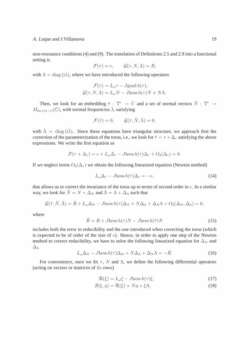
non-resonance conditions (4) and (9). The translation of Definitions 2.5 and 2.9 into a functionalsetting is
F(τ) = e, G(τ,N, Λ) = R,
with Λ = diag (iλ), where we have introduced the following operators
F(τ) = Lωτ − Jgrad h(τ),
G(τ,N, Λ) = LωN − Jhess h(τ)N + NΛ.
Then, we look for an embeddingτ : Tr → U and a set of normal vectorsN : T
r →M2n×(n−r)(C), with normal frequenciesλ, satisfying
F(τ) = 0, G(τ , N , Λ) = 0,
with Λ = diag (iλ). Since these equations have triangular structure, we approach first thecorrection of the parameterization of the torus, i.e., we look for τ = τ +∆τ satisfying the aboveexpressions. We write the first equation as
F(τ + ∆τ ) = e + Lω∆τ − Jhess h(τ)∆τ + O2(∆τ ) = 0.
If we neglect termsO2(∆τ ) we obtain the following linearized equation (Newton method)
Lω∆τ − Jhess h(τ)∆τ = −e, (14)
that allows us to correct the invariance of the torus up to terms of second order ine. In a similarway, we look forN = N + ∆N andΛ = Λ + ∆Λ such that
G(τ , N , Λ) = R + Lω∆N − Jhess h(τ)∆N + N∆Λ + ∆NΛ + O2(∆N , ∆Λ) = 0,
whereR = R + Jhess h(τ)N − Jhess h(τ)N (15)
includes both the error in reducibility and the one introduced when correcting the torus (whichis expected to be of order of the size ofe). Hence, in order to apply one step of the Newtonmethod to correct reducibility, we have to solve the following linearized equation for∆N and∆Λ
Lω∆N − Jhess h(τ)∆N + N∆Λ + ∆NΛ = −R. (16)
For convenience, once we fixτ , N andΛ, we define the following differential operators(acting on vectors or matrices of2n rows)
R(ξ) = Lωξ − Jhess h(τ)ξ, (17)
S(ξ, η) = R(ξ) + Nη + ξΛ, (18)
20 KAM theorem without action-angle for elliptic tori
so Equations (14) and (16) are equivalent to invertR andS
R(∆τ ) = −e, S(∆N , ∆Λ) = −R. (19)
As it was done in [13], the main idea is to use the geometric properties of the problemto prove that the linearized Equation (14) can be transformed, using a suitable basis alongthe approximate torus, into a simpler linear equation —withconstant coefficients— that can beapproximately solved by means of Fourier series. Indeed, anapproximate solution with an errorof quadratic size ine andR is enough for the convergence of the scheme —the Newton methodstill converges quadratically if we have a good enough approximation of the Jacobian matrix.Under suitable conditions of non-resonance and non-degeneracy, iteration of this process leadsto a quadratic scheme that allows us to overcome the effect ofthe small divisors of the problem.The main contribution of this paper is to adapt this construction (that we describe next in a moreprecise way) to deal with Equations (14) and (16) simultaneously.
Let us discuss the construction of the basis mentioned above. In the Lagrangian case weonly have to deal with Equation (14) and the columns of the matricesDτ andJDτG−1
Dτ give usan approximately symplectic basis ofR
2n at any point of the torus. Moreover, it turns out thatR(Dτ) = 0 +O(e) andR(JDτG−1
Dτ ) = DτA1 +O(e), whereA1 : Tn → Mn×n(R) is a sym-
metric matrix. Using this basis we can write the linearized equation (14) in “triangular form”with respect to the projections of∆τ overDτ andJDτG−1
Dτ , in such a way that the problemis reduced to solve two cohomological equations with constant coefficients. However, in thelower dimensional case the previous construction is not enough since we also have to take intoaccount the normal directions of the torus. As mentioned in the introduction, this scheme hasbeen recently adapted in [20] for the normally hyperbolic case, without requiring reducibility ofthe normal variational equations. The main ingredient is that there exists a splitting between thecenter and the hyperbolic directions of the torus and we can reduce the study of Equation (14)to the projections according to this splitting. The dynamics on the hyperbolic directions is char-acterized by asymptotic (geometric) growth conditions2 —both in the future and in the past—and the linearized equation (14) restricted to the center subspace follows as in the Lagragiancase (now the ambient space isR
2r).In the normally elliptic context, we ask for reducibility inorder to express equation (14) in a
simple form. Hence, we solve simultaneously equation (16),thus obtaining a basis that reducesthe normal variational equations of the torus to constants coefficients up to a quadratic error.In this case, the approximately (with an error of the order ofthe size ofe andR) symplecticbasis is obtained by completing the columns ofDτ , N andiN∗ with the columns of a suitablyconstructed matrixV : T
r → M2n×r(R). Basically, we take advantage of the fact thatVsatisfiesR(V ) = DτA1 modulo terms of ordere andR, whereA1 : T
r → Mr×r(R) will bespecified later on. Hence, we find approximately solutions for equations (19) in terms of the
2Concretely, the solution for the equations projected into the hyperbolic directions are obtained by means ofabsolutely convergent power series. See details in [20].
A. Luque and J.Villanueva 21
constructed basis as follows
∆τ = Dτ∆1 + V ∆2 + N∆3 + iN∗∆4,
∆N = DτP1 + V P2 + NP3 + iN∗P4,
where∆i, Pi, with i = 1, . . . , 4, are the solutions of cohomological equations (37)-(40),and (42)-(45), respectively. The correction∆Λ in the normal eigenvalues is determined fromthe compatibility condition of these last equations.
Let us observe that in order to correct the reducibility of the torus we have to change slightlythe normal directions and the normal frequencies. Since thenormal frequenciesλ are modifiedat each step of the process, we do not know in advance if they will satisfy the required Diophan-tine conditions for all steps —unless we have enough parameters to control the value of all ofthem simultaneously. To deal with this problem we require some control on the change of thesefrequencies, in such a way that we can remove parameters thatgive rise to resonant frequencies.Since at every step of the inductive process we are removing adense set of parameters, this doesnot allow us to keep any kind of smooth dependence with respect to them (because now theymove on a set of empty interior).
There are several methods in the literature to deal with thisproblem. The first approachwas due to Arnold (see [1]) and it consists in working, at every step of the inductive procedure,with a finite number of terms in the Fourier expansions (“ultraviolet cut-off”). Then, sincewe only need to deal with a finite number of resonances at everystep, we can work on opensets of parameters and keep the smooth dependence on these sets. Another possibility is toconsider Lipschitz parametric dependence and to check thatthis dependence is preserved alongthe iterative procedure (this is the method used in [33, 34, 35, 36]). Lipschitz regularity sufficesto control the measure of the resonant sets. In this paper we follow the Lipschitz approachbecause it does not forces to modify, by the effect of the “ultraviolet cut-off”, the geometricconstruction we have developed in the Diophantine case.
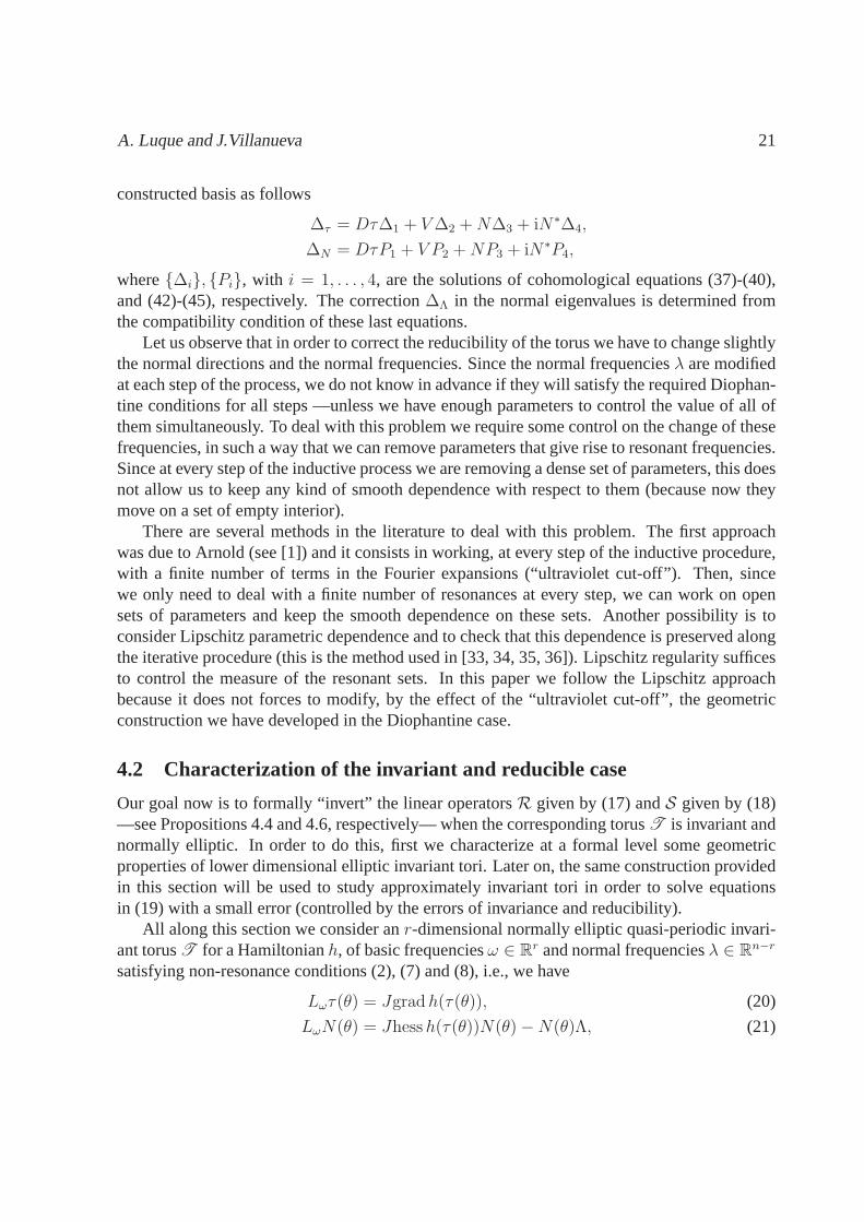
4.2 Characterization of the invariant and reducible case
Our goal now is to formally “invert” the linear operatorsR given by (17) andS given by (18)—see Propositions 4.4 and 4.6, respectively— when the corresponding torusT is invariant andnormally elliptic. In order to do this, first we characterizeat a formal level some geometricproperties of lower dimensional elliptic invariant tori. Later on, the same construction providedin this section will be used to study approximately invariant tori in order to solve equationsin (19) with a small error (controlled by the errors of invariance and reducibility).
All along this section we consider anr-dimensional normally elliptic quasi-periodic invari-ant torusT for a Hamiltonianh, of basic frequenciesω ∈ R
r and normal frequenciesλ ∈ Rn−r
satisfying non-resonance conditions (2), (7) and (8), i.e., we have
Lωτ(θ) = Jgrad h(τ(θ)), (20)
LωN(θ) = Jhess h(τ(θ))N(θ) − N(θ)Λ, (21)
22 KAM theorem without action-angle for elliptic tori
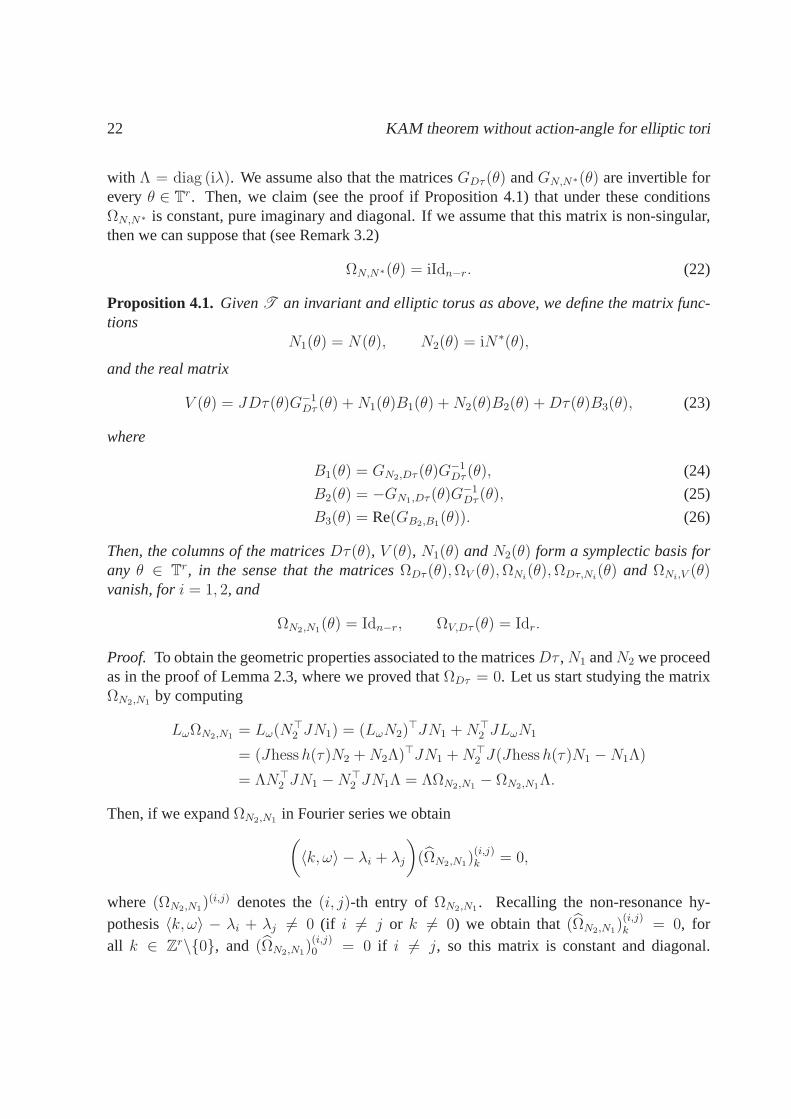
with Λ = diag (iλ). We assume also that the matricesGDτ (θ) andGN,N∗(θ) are invertible foreveryθ ∈ T
r. Then, we claim (see the proof if Proposition 4.1) that underthese conditionsΩN,N∗ is constant, pure imaginary and diagonal. If we assume that this matrix is non-singular,then we can suppose that (see Remark 3.2)
ΩN,N∗(θ) = iIdn−r. (22)
Proposition 4.1. GivenT an invariant and elliptic torus as above, we define the matrix func-tions
N1(θ) = N(θ), N2(θ) = iN∗(θ),
and the real matrix
V (θ) = JDτ(θ)G−1Dτ (θ) + N1(θ)B1(θ) + N2(θ)B2(θ) + Dτ(θ)B3(θ), (23)
where
B1(θ) = GN2,Dτ (θ)G−1Dτ (θ), (24)
B2(θ) = −GN1,Dτ (θ)G−1Dτ (θ), (25)
B3(θ) = Re(GB2,B1(θ)). (26)
Then, the columns of the matricesDτ(θ), V (θ), N1(θ) andN2(θ) form a symplectic basis forany θ ∈ T
r, in the sense that the matricesΩDτ (θ), ΩV (θ), ΩNi(θ), ΩDτ,Ni
(θ) and ΩNi,V (θ)vanish, fori = 1, 2, and
ΩN2,N1(θ) = Idn−r, ΩV,Dτ (θ) = Idr.
Proof. To obtain the geometric properties associated to the matricesDτ , N1 andN2 we proceedas in the proof of Lemma 2.3, where we proved thatΩDτ = 0. Let us start studying the matrixΩN2,N1 by computing
LωΩN2,N1 = Lω(N⊤2 JN1) = (LωN2)
⊤JN1 + N⊤2 JLωN1
= (Jhess h(τ)N2 + N2Λ)⊤JN1 + N⊤2 J(Jhess h(τ)N1 − N1Λ)
= ΛN⊤2 JN1 − N⊤
2 JN1Λ = ΛΩN2,N1 − ΩN2,N1Λ.
Then, if we expandΩN2,N1 in Fourier series we obtain(〈k, ω〉 − λi + λj
)(ΩN2,N1)
(i,j)k = 0,
where (ΩN2,N1)(i,j) denotes the(i, j)-th entry of ΩN2,N1. Recalling the non-resonance hy-
pothesis〈k, ω〉 − λi + λj 6= 0 (if i 6= j or k 6= 0) we obtain that(ΩN2,N1)(i,j)k = 0, for
all k ∈ Zr\0, and (ΩN2,N1)
(i,j)0 = 0 if i 6= j, so this matrix is constant and diagonal.
A. Luque and J.Villanueva 23
Moreover,Ω⊤N2,N1
= Ω∗N2,N1
so its entries are real. Finally, using hypothesis (22) we writeΩN2,N1 = iΩN∗,N = −iΩ⊤
N,N∗ = Idn−r.To prove thatΩN1 vanishes we compute
LωΩN1 = −ΛΩN1 − ΩN1Λ,
in a similar way as above. Now, the Fourier coefficients ofΩN1 satisfy(〈k, ω〉 + λi + λj
)(ΩN1)
(i,j)k = 0,
so it turns out that all of them vanish (using the non-resonance conditions). Moreover, takingderivatives at Equation (20) we obtain
LωDτ = Jhess hDτ,
that together with Equation (21), leads to
LωΩDτ,N1 = −ΩDτ,N1Λ,
which implies thatΩDτ,N1 = 0, since the Fourier coefficients of the component functions satisfythe equation (
〈k, ω〉 + λi
)(ΩDτ,N1)
(i,j)k = 0.
Finally, it is easy to see thatΩN2 = −Ω∗N1
andΩDτ,N2 = iΩ∗Dτ,N1
, so these matrices also vanish.Next, we see that the columns of the (real) matricesDτ , JDτG−1
Dτ , Re(N) and Im(N) formaR-basis ofR2n. To this end, it suffices to check that the columns ofDτ , JDτG−1
Dτ , N1 andN2
areC-independent onC2n. Thus, let us consider a linear combination
Dτa + JDτG−1Dτb + N1c + N2d = 0,
for vector functionsa, b : Tr → C
r andc, d : Tr → C
n−r. Multiplying by Dτ⊤, Dτ⊤J , N⊤2 J
andN⊤1 J and using the geometric properties proved above, we obtain the following system of
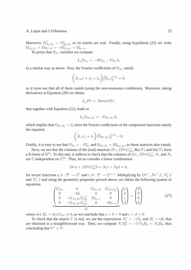
equations
GDτ 0 GDτ,N1 GDτ,N2
0 −Idr 0 00 −GN2,DτG
−1Dτ Idn−r 0
0 −GN1,DτG−1Dτ 0 −Idn−r
︸ ︷︷ ︸M1
abcd
=
0000
, (27)
wheredet M1 = det GDτ 6= 0, so we conclude thata = b = 0 andc = d = 0.To check that the matrixV is real, we use the expressionsN∗
1 = −iN2 andB∗1 = iB2 that
are obtained in a straightforward way. Then, we computeN∗1 B∗
1 = −i2N2B2 = N2B2, thusconcluding thatV ∗ = V .

24 KAM theorem without action-angle for elliptic tori
Finally, the following computations are straightforward
ΩDτ,V = − Idr + ΩDτ,N1B1 + ΩDτ,N2B2 + ΩDτB3 = −Idr,
ΩN1,V = − GN1,DτG−1Dτ + ΩN1B1 + ΩN1,N2B2 + ΩN1.DτB3
= − GN1,DτG−1Dτ − B2 = 0,
ΩN2,V = − GN2,DτG−1Dτ + B1 = 0,
ΩV = (G−1DτDτ⊤J⊤ + B⊤
1 N⊤1 + B⊤
2 N⊤2 + B⊤
3 Dτ⊤)JV
= G−1DτGDτ,N1B1 + G−1
DτGN2,DτB2 + B3 − B⊤3
= − GB2,B1 + GB1,B2 + B3 − B⊤3
= iIm(GB1,B2 − GB2,B1) = 0.
In the last computation we used thatV is real.
Remark 4.2. Notice that the matrixB3 can be taken modulo the addition of a symmetric realmatrix. This freedom can be used to ask for reducibility alsoin the “central directions” of thetorus. Hence, instead of the matrixA1 that appears in Lemma 4.3 we would obtain its average[A1]Tr . Since this does not give us any significant advantage, we do not resort to this fact.
In the invariant and reducible case, we characterize the action of R on Dτ(θ), N1(θ) andN2(θ) in a very simple way
R(Dτ(θ)) = 0, R(N1(θ)) = −N1(θ)Λ, R(N2(θ)) = N2(θ)Λ. (28)
The first expression follows immediately from equation (20)—invariance— and the other onesfrom equation (21) —reducibility. Moreover, we have the following result forV (θ).
Lemma 4.3. Under the setting of Proposition 4.1, we have that
R(V (θ)) = Dτ(θ)A1(θ),
whereA1 : Tr → Mr×r(R) is given by the real symmetric matrix
A1(θ) = G−1Dτ (θ)Dτ(θ)⊤(T1(θ) + T2(θ) + T2(θ)
⊤)Dτ(θ)G−1Dτ (θ), (29)
where
T1(θ) = J⊤hess h(τ(θ))J − hess h(τ(θ)), (30)
T2(θ) = T1J [Dτ(θ)GDτ (θ)−1Dτ(θ)⊤ − Id] Re(N1(θ)N2(θ)
⊤).
A. Luque and J.Villanueva 25
Proof. We only have to write the expression forR(V ) in terms of the previously constructedsymplectic basis
R(V ) = DτA1 + V A2 + N1A3 + N2A4, (31)
and then to show thatA1 is given by (29) andA2 = A3 = A4 = 0. First, we use (23) and (28)to expressR(V ) as
R(V ) = R(JDτG−1Dτ ) + N1(LωB1 − ΛB1) + N2(LωB2 + ΛB2) + DτLωB3.
Then, multiplying at both sides of equation (31) byV ⊤J , Dτ⊤J , N⊤2 J , N⊤
1 J and using thesymplectic properties of the basis we obtain the following expressions:
A1 = LωB3 + V ⊤JR(JDτG−1Dτ ), (32)
A2 = −Dτ⊤JR(JDτG−1Dτ ), (33)
A3 = LωB1 − ΛB1 + N⊤2 JR(JDτG−1
Dτ ), (34)
A4 = LωB2 + ΛB2 − N⊤1 JR(JDτG−1
Dτ ). (35)
First, introducingB1 = GN2,DτG−1Dτ into equation (34), we obtain
A3 = Lω(N⊤2 DτG−1
Dτ ) − ΛN⊤2 DτG−1
Dτ + N⊤2 JR(JDτG−1
Dτ )
= LωN⊤2 DτG−1
Dτ + N⊤2 Lω(DτG−1
Dτ ) − ΛN⊤2 DτG−1
Dτ
+ N⊤2 JLω(JDτG−1
Dτ ) + N⊤2 hess hJDτG−1
Dτ
= (LωN2 − Jhess hN2︸ ︷︷ ︸R(N2)
−N2Λ)⊤DτG−1Dτ = 0,
where we used the property (28) forN2. Recalling thatN2 = iN∗1 we observe thatA∗
3 = iA4 sowe also haveA4 = 0.
Now, we expand the expression forR(JDτG−1Dτ ), obtaining
R(JDτG−1Dτ ) = R(JDτ)G−1
Dτ + JDτLω(G−1Dτ )
= − hess hDτG−1Dτ − JDτG−1
Dτ (Dτ⊤Jhess h − Dτ⊤hess hJ)DτG−1Dτ
− Jhess hJDτG−1Dτ = (Idr + JDτG−1
DτDτ⊤J)T1DτG−1Dτ ,
where we used expression (30) forT1. Then, on the one hand we haveDτ⊤JR(JDτG−1Dτ ) = 0
—in combination with (33) this implies thatA2 = 0— and on the other hand we have
V ⊤JR(JDτG−1Dτ ) = (B⊤
3 Dτ⊤ + B⊤2 N⊤
2 + B⊤1 N⊤
1 + G−1DτDτ⊤J⊤)JR(JDτG−1
Dτ )
= − B⊤2 (LωB1 − ΛB1) + B⊤
1 (LωB2 + ΛB2) + G−1DτDτ⊤T1DτG−1
Dτ ,
26 KAM theorem without action-angle for elliptic tori
where we have used equations (34) and (35) taking into account thatA3 = A4 = 0. Finally, weintroduce this last expression into (32) and recall thatB3 = Re(GB2,B1) in order to obtain
A1 = Re(Lω(B⊤2 B1)) − B⊤
2 (LωB1 − ΛB1) + B⊤1 (LωB2 + ΛB2) + G−1
DτDτ⊤T1DτG−1Dτ
= Re(LωB⊤2 B1 − B⊤
2 LωB1 + 2B⊤2 ΛB1) + G−1
DτDτ⊤T1DτG−1Dτ ,
where we used that(B⊤1 (LωB2 + ΛB2))
∗ = −B⊤2 (LωB1 − ΛB1). Now we replaceB1 andB2
by equations (24) and (25) respectively, and we expand the expression forLωB1 andLωB2 asfollows (we also use thatB1 = −iB∗
2)
LωB2 = − LωN⊤1 DτG−1
Dτ − N⊤1 Lω(DτG−1
Dτ )
= ΛN⊤1 DτG−1
τ − N⊤1 hess hJ⊤DτG−1
Dτ − N⊤1 Lω(DτG−1
Dτ )
= − ΛB2 + N⊤1 JT1DτG−1
Dτ − N⊤1 DτLω(G−1
Dτ )
= − ΛB2 + N⊤1 JT1DτG−1
Dτ − N⊤1 DτG−1
DτDτ⊤JT1DτG−1Dτ .
LωB1 = ΛB1 − N⊤2 JT1DτG−1
Dτ + N⊤2 DτG−1
DτDτ⊤JT1DτG−1Dτ .
From this expressions we observe that term2B⊤2 ΛB1 in A1 is cancelled. Finally, since(N1N
⊤2 )∗ =
−N2N⊤1 = (−N1N
⊤2 )⊤, it turns out that Re(N1N
⊤2 ) = Re((−N1N
⊤2 )⊤) so we obtain the ex-
pression (29) forA1.
Now we have all the ingredients for inverting formally the operatorR.
Proposition 4.4. Under the setting of Proposition 4.1, we assume that the matrix A1 givenin (29) satisfies the twist conditiondet [A1]Tr 6= 0. Then, given a functione : T
r → R2n
satisfying[Dτ⊤Je
]Tr = 0, we obtain a formal solution for the equation
R(∆τ (θ)) = Lω∆τ − Jhess h(τ)∆τ = −e(θ),
which is unique up to terms inker(R) = DτA : A ∈ Mr×r(R).
Proof. We express the unknown∆τ (θ) in terms of the constructed symplectic basis
∆τ = Dτ∆1 + V ∆2 + N1∆3 + N2∆4, (36)
expandR(∆τ ) and project to compute the functions∆ii=1,...,4. Concretely, we have
R(∆τ ) = R(Dτ)∆1 + R(V )∆2 + R(N1)∆3 + R(N2)∆4
+ DτLω∆1 + V Lω∆2 + N1Lω∆3 + N2Lω∆4
= Dτ(Lω∆1 + A1∆2) + V Lω∆2 + N1(Lω∆3 − Λ∆3) + N2(Lω∆4 + Λ∆4).
A. Luque and J.Villanueva 27
Multiplying at both sides of this expression byV ⊤J , Dτ⊤J , N⊤2 J andN⊤
1 J , we obtain thefollowing four cohomological equations:
Lω∆1 + A1∆2 = −V ⊤Je, (37)
Lω∆2 = Dτ⊤Je, (38)
Lω∆3 − Λ∆3 = −N⊤2 Je, (39)
Lω∆4 + Λ∆4 = N⊤1 Je. (40)
As[Dτ⊤Je
]Tr = 0, the solution of equation (38) is unique, up to an arbitrary average
[∆2]Tr , provided that the non-resonance condition (2) holds. Then, using the non-degeneracyconditiondet [A1]Tr 6= 0, we choose
[∆2]Tr = [A1]−1Tr
([−V ⊤Je
]Tr −
[A1∆2
]Tr
)(41)
in such a way that[A1∆2 + V ⊤Je
]Tr = 0 so we have a unique solution for∆1 up to the
freedom of fixing[∆1]Tr . Actually, it is easy to check (39) and (40) have unique solution for∆3 and∆4 provided that the non-resonance condition (9) is fulfilled.Moreover, sincee is a realfunction, we conclude that∆∗
3 = i∆4 and this allows us to guarantee that the expression (36) isalso real.
Remark 4.5. We will see that the compatibility condition[Dτ⊤Je
]Tr = 0 is automatically
fulfilled if τ parametrices and approximately invariant torus,e being the error of invariance—see computations in(93).
Proposition 4.6.Under the setting of Proposition 4.1, given a functionR : Tr 7→ M2n×(n−r)(C),
we obtain a solution for the equation
S(∆N , ∆Λ) = R(∆N) + N∆Λ + ∆NΛ = −R,
which is unique for∆Λ and for∆N up to terms inker(S) = ND : D = diag (d), d ∈ Cn−r.
Proof. As before, we write the solution∆N of this equation in terms of the symplectic basis as
∆N = DτP1 + V P2 + N1P3 + N2P4.
Then, we compute the action ofS on the pair(∆N , ∆Λ), thus obtaining
S(∆N , ∆Λ) = R(∆N) + N1∆Λ + ∆NΛ
= R(Dτ)P1 + R(V )P2 + R(N1)P3 + R(N2)P4
+ DτLωP1 + V LωP2 + N1LωP3 + N2LωP4 + N1∆Λ
+ DτP1Λ + V P2Λ + N1P3Λ + N2P4Λ
28 KAM theorem without action-angle for elliptic tori
= Dτ(LωP1 + P1Λ + A1P2) + V (LωP2 + P2Λ)
+ N1(LωP3 + P3Λ − ΛP3 + ∆Λ) + N2(LωP4 + P4Λ + ΛP4) = R.
If we multiply this expression byV ⊤J , Dτ⊤J , N⊤2 J andN⊤
1 J , we end up with the follow-ing four cohomological equations:
LωP1 + P1Λ + A1P2 = −V ⊤JR, (42)
LωP2 + P2Λ = Dτ⊤JR, (43)
LωP3 + P3Λ − ΛP3 = −N⊤2 JR − ∆Λ, (44)
LωP4 + P4Λ + ΛP4 = N⊤1 JR. (45)
Let us observe that, under the assumed non-resonance conditions (7) and (8), the only un-avoidable resonances are those in the diagonal of the average of equation (44), so we requirethat the diagonal of the average of the right-hand side of this equation vanishes. This is attainedby fixing the correction of the normal eigenvalues∆Λ = −diag [N⊤
2 JR]Tr . Therefore, we ob-tain a unique solutionP1, P2, P3, P4 and∆Λ —modulo terms indiag [P3]Tr— of this system ofequations.
Remark 4.7. We will see that ifR corresponds to the error in reducibility as defined in equa-tion (15) then the geometry imposes that the correction∆Λ is a pure imaginary diagonal matrix,thus preserving the elliptic normal behavior —see computations in(96).
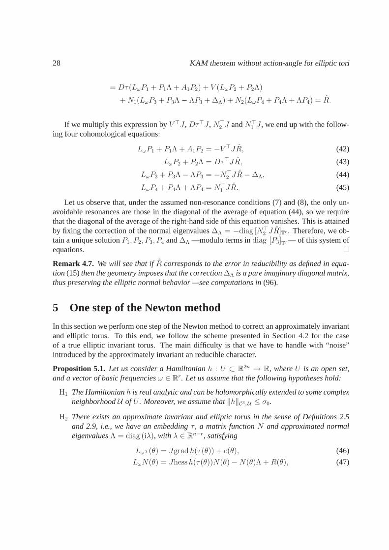
5 One step of the Newton method
In this section we perform one step of the Newton method to correct an approximately invariantand elliptic torus. To this end, we follow the scheme presented in Section 4.2 for the caseof a true elliptic invariant torus. The main difficulty is that we have to handle with “noise”introduced by the approximately invariant an reducible character.
Proposition 5.1. Let us consider a Hamiltonianh : U ⊂ R2n → R, whereU is an open set,
and a vector of basic frequenciesω ∈ Rr. Let us assume that the following hypotheses hold:
H1 The Hamiltonianh is real analytic and can be holomorphically extended to somecomplexneighborhoodU of U . Moreover, we assume that‖h‖C3,U ≤ σ0.
H2 There exists an approximate invariant and elliptic torus inthe sense of Definitions 2.5and 2.9, i.e., we have an embeddingτ , a matrix functionN and approximated normaleigenvaluesΛ = diag (iλ), with λ ∈ R
n−r, satisfying
Lωτ(θ) = Jgrad h(τ(θ)) + e(θ), (46)
LωN(θ) = Jhess h(τ(θ))N(θ) − N(θ)Λ + R(θ), (47)
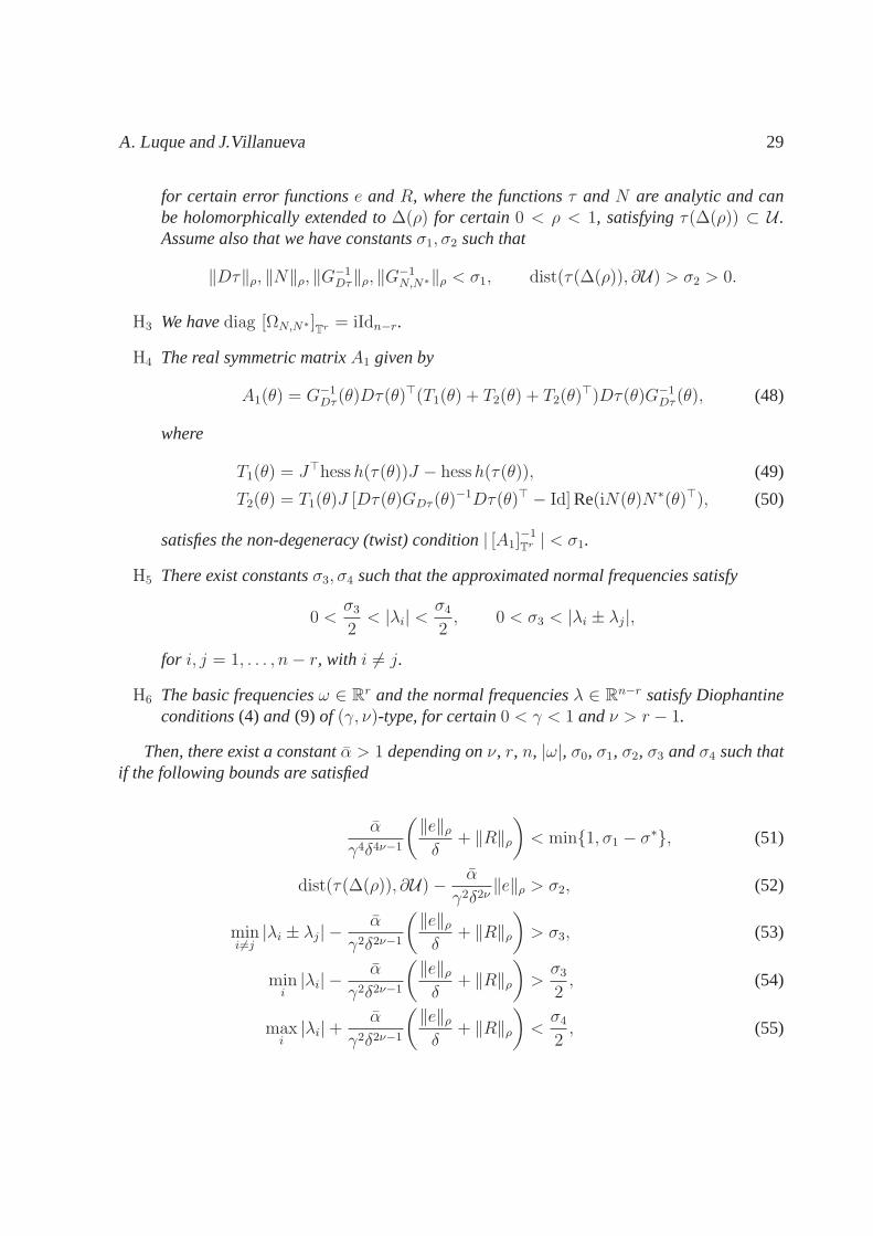
A. Luque and J.Villanueva 29
for certain error functionse andR, where the functionsτ andN are analytic and canbe holomorphically extended to∆(ρ) for certain 0 < ρ < 1, satisfyingτ(∆(ρ)) ⊂ U .Assume also that we have constantsσ1, σ2 such that
‖Dτ‖ρ, ‖N‖ρ, ‖G−1Dτ‖ρ, ‖G
−1N,N∗‖ρ < σ1, dist(τ(∆(ρ)), ∂U) > σ2 > 0.
H3 We havediag [ΩN,N∗ ]Tr = iIdn−r.
H4 The real symmetric matrixA1 given by
A1(θ) = G−1Dτ (θ)Dτ(θ)⊤(T1(θ) + T2(θ) + T2(θ)
⊤)Dτ(θ)G−1Dτ (θ), (48)
where
T1(θ) = J⊤hess h(τ(θ))J − hess h(τ(θ)), (49)
T2(θ) = T1(θ)J [Dτ(θ)GDτ (θ)−1Dτ(θ)⊤ − Id] Re(iN(θ)N∗(θ)⊤), (50)
satisfies the non-degeneracy (twist) condition| [A1]−1Tr | < σ1.
H5 There exist constantsσ3, σ4 such that the approximated normal frequencies satisfy
0 <σ3
2< |λi| <
σ4
2, 0 < σ3 < |λi ± λj|,
for i, j = 1, . . . , n − r, with i 6= j.
H6 The basic frequenciesω ∈ Rr and the normal frequenciesλ ∈ R
n−r satisfy Diophantineconditions(4) and (9) of (γ, ν)-type, for certain0 < γ < 1 andν > r − 1.
Then, there exist a constantα > 1 depending onν, r, n, |ω|, σ0, σ1, σ2, σ3 andσ4 such thatif the following bounds are satisfied
α
γ4δ4ν−1
(‖e‖ρ
δ+ ‖R‖ρ
)< min1, σ1 − σ∗, (51)
dist(τ(∆(ρ)), ∂U) −α
γ2δ2ν‖e‖ρ > σ2, (52)
mini6=j
|λi ± λj| −α
γ2δ2ν−1
(‖e‖ρ
δ+ ‖R‖ρ
)> σ3, (53)
mini
|λi| −α
γ2δ2ν−1
(‖e‖ρ
δ+ ‖R‖ρ
)>
σ3
2, (54)
maxi
|λi| +α
γ2δ2ν−1
(‖e‖ρ
δ+ ‖R‖ρ
)<
σ4
2, (55)
30 KAM theorem without action-angle for elliptic tori
whereσ∗ = max
‖Dτ‖ρ, ‖N‖ρ, ‖G
−1Dτ‖ρ, ‖G
−1N,N∗‖ρ, | [A1]
−1Tr |
,
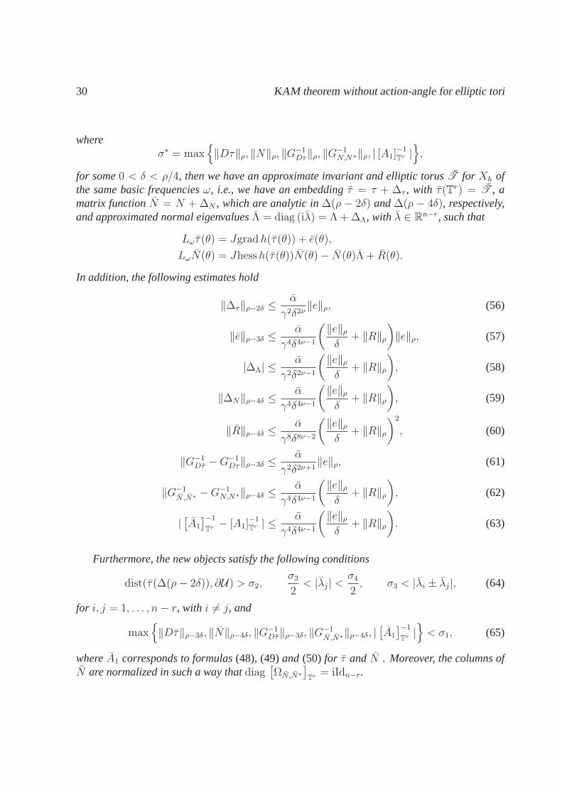
for some0 < δ < ρ/4, then we have an approximate invariant and elliptic torusT for Xh ofthe same basic frequenciesω, i.e., we have an embeddingτ = τ + ∆τ , with τ(Tr) = T , amatrix functionN = N + ∆N , which are analytic in∆(ρ − 2δ) and∆(ρ − 4δ), respectively,and approximated normal eigenvaluesΛ = diag (iλ) = Λ + ∆Λ, with λ ∈ R
n−r, such that
Lω τ(θ) = Jgrad h(τ(θ)) + e(θ),
LωN(θ) = Jhess h(τ(θ))N(θ) − N(θ)Λ + R(θ).
In addition, the following estimates hold
‖∆τ‖ρ−2δ ≤α
γ2δ2ν‖e‖ρ, (56)
‖e‖ρ−3δ ≤α
γ4δ4ν−1
(‖e‖ρ
δ+ ‖R‖ρ
)‖e‖ρ, (57)
|∆Λ| ≤α
γ2δ2ν−1
(‖e‖ρ
δ+ ‖R‖ρ
), (58)
‖∆N‖ρ−4δ ≤α
γ4δ4ν−1
(‖e‖ρ
δ+ ‖R‖ρ
), (59)
‖R‖ρ−4δ ≤α
γ8δ8ν−2
(‖e‖ρ
δ+ ‖R‖ρ
)2
, (60)
‖G−1Dτ − G−1
Dτ‖ρ−3δ ≤α
γ2δ2ν+1‖e‖ρ, (61)
‖G−1N,N∗
− G−1N,N∗‖ρ−4δ ≤
α
γ4δ4ν−1
(‖e‖ρ
δ+ ‖R‖ρ
), (62)
|[A1
]−1
Tr − [A1]−1Tr | ≤
α
γ4δ4ν−1
(‖e‖ρ
δ+ ‖R‖ρ
). (63)
Furthermore, the new objects satisfy the following conditions
dist(τ(∆(ρ − 2δ)), ∂U) > σ2,σ3
2< |λj| <
σ4
2, σ3 < |λi ± λj|, (64)
for i, j = 1, . . . , n − r, with i 6= j, and
max‖Dτ‖ρ−3δ, ‖N‖ρ−4δ, ‖G
−1Dτ‖ρ−3δ, ‖G
−1N ,N∗
‖ρ−4δ, |[A1
]−1
Tr |
< σ1, (65)
whereA1 corresponds to formulas(48), (49) and (50) for τ andN . Moreover, the columns ofN are normalized in such a way thatdiag
[ΩN ,N∗
]Tr = iIdn−r.
A. Luque and J.Villanueva 31
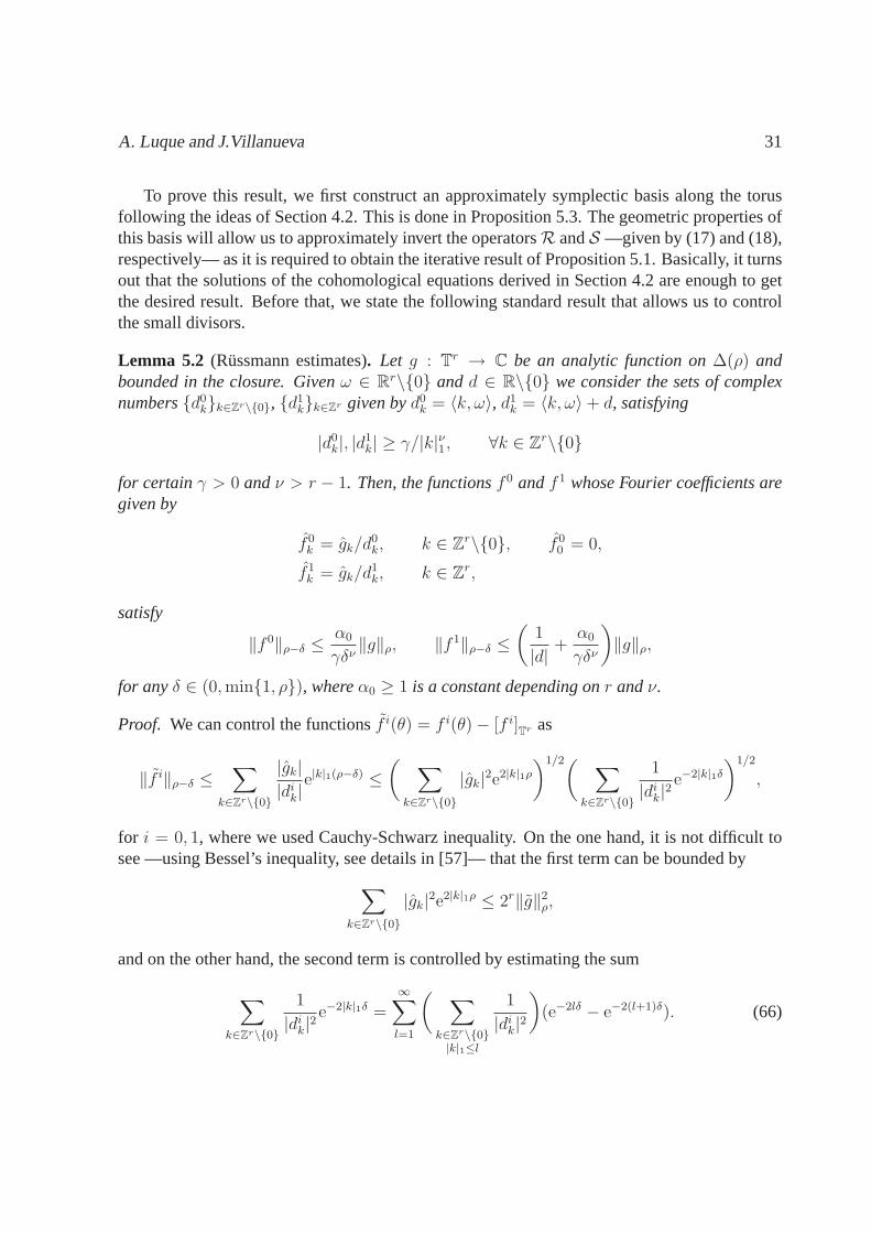
To prove this result, we first construct an approximately symplectic basis along the torusfollowing the ideas of Section 4.2. This is done in Proposition 5.3. The geometric properties ofthis basis will allow us to approximately invert the operatorsR andS —given by (17) and (18),respectively— as it is required to obtain the iterative result of Proposition 5.1. Basically, it turnsout that the solutions of the cohomological equations derived in Section 4.2 are enough to getthe desired result. Before that, we state the following standard result that allows us to controlthe small divisors.
Lemma 5.2 (Russmann estimates). Let g : Tr → C be an analytic function on∆(ρ) and
bounded in the closure. Givenω ∈ Rr\0 andd ∈ R\0 we consider the sets of complex
numbersd0kk∈Zr\0, d1
kk∈Zr given byd0k = 〈k, ω〉, d1
k = 〈k, ω〉 + d, satisfying
|d0k|, |d
1k| ≥ γ/|k|ν1, ∀k ∈ Z
r\0
for certainγ > 0 andν > r − 1. Then, the functionsf 0 andf 1 whose Fourier coefficients aregiven by
f 0k = gk/d
0k, k ∈ Z
r\0, f 00 = 0,
f 1k = gk/d
1k, k ∈ Z
r,
satisfy
‖f 0‖ρ−δ ≤α0
γδν‖g‖ρ, ‖f 1‖ρ−δ ≤
(1
|d|+
α0
γδν
)‖g‖ρ,
for anyδ ∈ (0, min1, ρ), whereα0 ≥ 1 is a constant depending onr andν.
Proof. We can control the functionsf i(θ) = f i(θ) − [f i]Tr as
‖f i‖ρ−δ ≤∑
k∈Zr\0
|gk|
|dik|
e|k|1(ρ−δ) ≤
( ∑
k∈Zr\0
|gk|2e2|k|1ρ
)1/2( ∑
k∈Zr\0
1
|dik|
2e−2|k|1δ
)1/2
,
for i = 0, 1, where we used Cauchy-Schwarz inequality. On the one hand, itis not difficult tosee —using Bessel’s inequality, see details in [57]— that thefirst term can be bounded by
∑
k∈Zr\0
|gk|2e2|k|1ρ ≤ 2r‖g‖2
ρ,
and on the other hand, the second term is controlled by estimating the sum
∑
k∈Zr\0
1
|dik|
2e−2|k|1δ =
∞∑
l=1
( ∑
k∈Zr\0
|k|1≤l
1
|dik|
2
)(e−2lδ − e−2(l+1)δ). (66)

32 KAM theorem without action-angle for elliptic tori
Now, we study in detail the case ofd1k (the case ofd0
k is analogous). First, we observe that thedivisorsd1
k = 〈k, ω〉 + d satisfydk1 6= dk2 if k1 6= k2. Then, givenl ∈ N, we define
Dl = k ∈ Zr\0 : |k|1 ≤ l andd1
k > 0
and we sort the divisors according to0 < dk1 < . . . < dk#Dlwith kj ∈ Dl, for j = 1, . . . , #Dl.
Then, we observe that (since|kj − kj−1| ≤ 2l)
d1kj− d1
kj−1= |〈kj − kj−1, ω〉| ≥ d0
2l,min, (67)
where the have introduced the notation
dil,min = min
k∈Zr\0
|k|1≤l
|dik|.
From expression (67) we obtain recursively
d1kj
= d1kj−1
+ d1kj− d1
kj−1≥ d1
kj−1+ d0
2l,min ≥ d1l,min + (j − 1)d0
2l,min.
Then, using thatd02l,min ≥ γ/(2l)ν andd1
l,min ≥ γ/lν , we have
#Dl∑
j=1
1
(d1kj
)2≤
#Dl∑
j=1
1
(d1l,min + (j − 1)d0
2l,min)2≤
∞∑
j=1
l2ν
γ2(1 + (j − 1)2−ν)2≤
α(ν)
γ2l2ν ,
and using a similar argument ford1kj
< 0, we obtain
∑
k∈Zr\0
|k|1≤l
1
|d1k|
2≤
2α(ν)
γ2l2ν ,
so we can control the sum (66) as follows
∑
k∈Zr\0
1
|dik|
2e−2|k|1δ ≤
∞∑
l=1
2δα(ν)
γ2
∫ l+1
l
x2νe−2δxdx ≤α(ν)
γ2(2δ)2νΓ(2ν + 1).
Combining the obtained expressions —and using that| [f 1]Tr | = |g0|/|d|— we end up with the
stated estimates.
Proposition 5.3. Under the same notations and assumptions of Proposition 5.1, we define thematrix functions
N1(θ) = N(θ), N2(θ) = iN∗(θ),
A. Luque and J.Villanueva 33
and the real analytic matrixV (θ) given by(23)-(26). Then, for any0 < δ < ρ/2 the followingestimates hold:
‖ΩDτ‖ρ−2δ ≤α
γδν+1‖e‖ρ, (68)
‖ΩNi‖ρ−δ ≤
α
γδν‖R‖ρ, (69)
‖ΩDτ,Ni‖ρ−2δ ≤
α
γδν
(‖e‖ρ
δ+ ‖R‖ρ
), (70)
‖ΩN2,N1 − Idn−r‖ρ−δ ≤α
γδν‖R‖ρ, (71)
‖ΩV,Dτ − Idr‖ρ−2δ ≤α
γδν
(‖e‖ρ
δ+ ‖R‖ρ
), (72)
‖ΩV,Ni‖ρ−2δ ≤
α
γδν
(‖e‖ρ
δ+ ‖R‖ρ
), (73)
‖ΩV ‖ρ−2δ ≤α
γδν
(‖e‖ρ
δ+ ‖R‖ρ
), (74)
for i = 1, 2, whereα > 1 is a constant depending onν, r, n, |ω|, σ0, σ1, σ3 andσ4. Furthermore,if the errors‖e‖ρ and‖R‖ρ satisfy
α
γδν
(‖e‖ρ
δ+ ‖R‖ρ
)≤
1
2, (75)
then the columns ofDτ(θ), V (θ), N1(θ), N2(θ) form an approximately symplectic basis foreveryθ ∈ T
r. In addition, it turns out that the action of the operatorR given in(17) on V isexpressed in terms of this basis as
R(V (θ)) = Dτ(θ)(A1(θ) + A+1 (θ)) + V (θ)A+
2 (θ) + N1(θ)A+3 (θ) + N2(θ)A
+4 (θ), (76)
whereA1 is the matrix(48)andA+1 , A+
2 , A+3 andA+
4 satisfy the estimate
‖A+i ‖ρ−2δ ≤
α
γδν+1
(‖e‖ρ
δ+ ‖R‖ρ
), (77)
for i = 1, . . . , 4.
Proof. For the sake of simplicity, we redefine (enlarge) the constant α along the proof to meetthe different conditions given in the statement. For example, we observe that there exist aconstantα > 0, depending onr, n, |ω|, σ0 andσ1, such that
‖Bi‖ρ, ‖T1‖ρ, ‖T2‖ρ, ‖A1‖ρ, ‖V ‖ρ ≤ α, ‖LωBi‖ρ−δ ≤α
δ, (78)
34 KAM theorem without action-angle for elliptic tori
for i = 1, 2, 3 —we recall thatT1 andT2 are given in (49) and (50), respectively. Now wetake derivatives at both sides of the approximated invariance equation in (46) and we read thereducibility equations in (47) forN1 andN2
LωDτ = Jhess h(τ)Dτ + De,
LωN1 = Jhess h(τ)N1 − N1Λ + R,
LωN2 = Jhess h(τ)N2 + N2Λ + iR∗. (79)
Using the previous expressions, we compute the derivateLω of the matricesΩDτ , ΩN1,ΩDτ,N1 andΩN2,N1 thus obtaining
Lω(ΩDτ ) = ΩDe,Dτ + ΩDτ,De, (80)
Lω(ΩN1) = −ΛΩN1 − ΩN1Λ + ΩR,N1 + ΩN1R, (81)
Lω(ΩDτ,N1) = −ΩDτ,N1Λ + ΩDe,N1 + ΩDτ,R, (82)
Lω(ΩN2,N1) = ΛΩN2,N1 − ΩN2,N1Λ + iΩR∗,N1 + ΩN2,R. (83)
First, we get estimate (68) forΩDτ by applying Lemma 5.2 to the(i, j)-component ofΩDτ
obtained from (80), i.e., takingd0k = 〈ω, k〉 andg = −i(ΩDe,Dτ +ΩDτ,De)
(i,j) that (using Cauchyestimates) is analytic in∆(ρ − δ). Moreover, since[ΩDτ ]Tr = 0 (see Remark 2.2), we obtain
‖ΩDτ‖ρ−2δ ≤α0
γδν‖g‖ρ−δ ≤
α
γδν+1‖e‖ρ.
Then, we proceed in a similar way to get (69) forN1, by applying Lemma 5.2 to the(i, j)-component ofΩN1 obtained from (81), i.e., takingd1
k = 〈ω, k〉 + λi + λj andg = −i(ΩR,N1 +ΩN1R)(i,j), analytic in∆(ρ). To bound the average ofΩN1 , we use hypothesisH5 of Proposi-tion 5.1.
‖ΩN1‖ρ−δ ≤
(1
mini,j |λi + λj|+
α0
γδν
)‖g‖ρ ≤
(1
σ3
+α0
γδν
)≤
α
γδν‖R‖ρ,
Analogous computations from Equations (82) and (83) allow us to obtain estimate (70) forN1
and (71). Of course, to obtain (71) we resort to the hypothesis diag [ΩN,N∗ ]Tr = iIdn−r in H3
of Proposition 5.1. The corresponding estimates (69) and (70) for N2 are straightforward usingthatΩN2 = −Ω∗
N1andΩDτ,N2 = iΩ∗
Dτ,N1.
Next we show that the columns ofDτ , JDτG−1Dτ , Re(N1) and Im(N1) form a R-basis of
R2n. As in the proof of Proposition 4.1, we consider a linear combination
Dτa + JDτG−1Dτb + N1c + N2d = 0,
A. Luque and J.Villanueva 35
for functionsa, b : Tr → C
r andc, d : Tr → C
n−r. We project this equation multiplying byDτ⊤, Dτ⊤J , N⊤
2 J andN⊤1 J , thus obtaining
M1 +
0 ΩDτG−1Dτ 0 0
ΩDτ 0 ΩDτ,N1 ΩDτ,N2
ΩN2,Dτ 0 ΩN2,N1 − Idn−r ΩN2
ΩN1,Dτ 0 ΩN1 ΩN1,N2 + Idn−r
︸ ︷︷ ︸M2
abcd
=
0000
,
whereM1 is the same matrix that appears in equation (27). Now, we haveto invert the matrixM1 + M2 = M1(Id + M−1
1 M2), where
M−11 =
G−1Dτ M1,2 −G−1
DτGDτ,N1 G−1DτGDτ,N2
0 −Idr 0 00 −GN2,DτG
−1Dτ Idn−r 0
0 GN1,DτG−1Dτ 0 −Idn−r
,
with M1,2 = G−1Dτ (GDτ,N1GN2,Dτ − GDτ,N2GN1,Dτ )G
−1Dτ , so it is clear that‖M−1
1 ‖ρ ≤ α. Bymeans of Neumann series we obtain
‖(Id + M−11 M2)
−1‖ρ−2δ ≤1
1 − ‖M−11 M2‖ρ−2δ
,
that it is well posed since (using bounds (68)-(71))
‖M−11 M2‖ρ−2δ ≤
α
γδν
(‖e‖ρ
δ+ ‖R‖ρ
)≤
1
2,
and applying hypothesis (75). Then, it must bea = b = 0 andc = d = 0 alongTr.
Now, we consider the basis defined by the columns ofDτ , V , N1 andN2, whereV is givenby (23)-(26), and we characterize the fact that the new basisis approximately symplectic. It isstraightforward to compute
ΩDτ,V = −Idr + ΩDτ,N1B1 + ΩDτ,N2B2 + ΩDτB3,
ΩN1,V = −GN1,DτG−1Dτ + ΩN1B1 + ΩN1,N2B2 + ΩN1,DτB3
= ΩN1B1 + (ΩN1,N2 + Idn−r)B2 + ΩN1,DτB3,
ΩV = B⊤3 (ΩDτ,V + Idr) + B⊤
1 ΩN1,V + B⊤2 ΩN2,V + G−1
DτΩDτG−1Dτ ,
andΩN2,V = iΩ∗N1,V . Then, estimates (72)-(74) follow from (68)-(71) and (78).
Let us characterize the action of the linear operatorR on the elements of this basis. Byhypothesis, we immediately have that
R(Dτ) = De, R(N1) = −N1Λ + R, R(N2) = N2Λ + iR∗, (84)
36 KAM theorem without action-angle for elliptic tori
and we have to see that if we write
R(V ) = Dτ(A1 + A+1 ) + V A+
2 + N1A+3 + N2A
+4 ,
whereA1 is the matrix (29), then the functionsA+1 , A+
2 , A+3 andA+
4 are small —i.e., theysatisfy (77). To this end, expandingR(V ) in the previous expression as
R(V ) = R(JDτG−1Dτ ) + N1(LωB1 − ΛB1) + N2(LωB2 + ΛB2) + DτLωB3
+ RB1 + iR∗B2 + DeB3,
and multiplying at both sides of this equation byV ⊤J , Dτ⊤J , N⊤2 J andN⊤
1 J , we obtain thelinear system
(Id + M3
)
A+1
A+2
A+3
A+4
=
C1
C2
C3
C4
, (85)
where
M3 =
ΩV,Dτ − Idr ΩV ΩV,N1 ΩV,N2
−ΩDτ ΩV,Dτ − Idr −ΩDτ,N1 −ΩDτ,N2
ΩN2,Dτ ΩN2,V ΩN2,N1 − Idn−r ΩN2
−ΩN1,Dτ −ΩN1,V −ΩN1 ΩN2,N1 − Idn−r
(86)
and the functionsC1, C2, C3 andC4 have the following form
C1 =
C+1︷ ︸︸ ︷
V ⊤JR(JDτG−1Dτ ) + LωB3 − A1 +ΩV,N1(LωB1 − ΛB1) + ΩV,N2(LωB2 + ΛB2)
+ V ⊤J(RB1 + iR∗B2 + DeB3) + (ΩV,Dτ − Idr)(LωB3 − A1),
C2 =
C+2︷ ︸︸ ︷
−Dτ⊤JR(JDτG−1Dτ )−ΩDτ,N1(LωB1 − ΛB1) − ΩDτ,N2(LωB2 + ΛB2)
− Dτ⊤J(RB1 + iR∗B2 + DeB3) + ΩDτ (A1 − LωB3),
C3 =
C+3︷ ︸︸ ︷
N⊤2 JR(JDτG−1
Dτ ) + LωB1 − ΛB1 +ΩN2(LωB2 + ΛB2) + ΩN2,Dτ (LωB3 − A1)
+ (ΩN2,N1 − Idn−r)(LωB1 − ΛB1) + N⊤2 J(RB1 + iR∗B2 + DeB3),
C4 =
C+4︷ ︸︸ ︷
−N⊤1 JR(JDτG−1
Dτ ) + LωB2 + ΛB2 −ΩN1(LωB1 − ΛB1) + ΩN1,Dτ (A1 − LωB3)
− (ΩN1,N2 + Idn−r)(LωB2 + ΛB2) − N⊤1 J(RB1 + iR∗B2 + DeB3),
A. Luque and J.Villanueva 37
and we observe thatC4 = −iC∗3 andC+
4 = −i(C+3 )∗. Apart fromC+
1 , C+2 , C+
3 andC+4 , the size
of the other terms that appear in the above expressions are easily controlled in terms of‖e‖ρ
and‖R‖ρ —using approximately symplectic properties in (68)-(74).We see next thatC+j , for
j = 1, . . . , 4, are also controlled in a similar way, since they are given byequation which areclose to (32)-(35) for the invariant and reducible case. Forexample, using equation (24) forB1
in the expressions ofC+3 we obtain
C+3 = (LωN2 − Jhess hN2 − N2Λ)⊤DτG−1
Dτ = iGR∗,DτG−1Dτ , (87)
where we used equation (79). To controlC+1 andC+
2 we have to compute the action ofR onthe matrixJDτG−1
Dτ
R(JDτG−1Dτ ) = R(JDτ)G−1
Dτ + JDτLω(G−1Dτ ) = (Id + JDτG−1
DτDτ⊤J)T1DτG−1Dτ
+ JDeG−1Dτ − JDτG−1
Dτ [GDe,Dτ + GDτ,De]G−1Dτ .
whereT1 is given by (49). Then, if we multiply this expression byDτ⊤J we get
C+2 = −GDe,DτG
−1Dτ (88)
and if we multiply byV ⊤J and use the definitions ofC+2 , C+
3 andC+4 , we obtain
C+1 = (B⊤
3 Dτ⊤ + B⊤2 N⊤
2 + B⊤1 N⊤
1 + G−1DτDτ⊤J⊤)JR(JDτG−1
Dτ ) + LωB3 − A1
= − B⊤3 C+
2 + B⊤2 (C+
3 − LωB1 + ΛB1) + B⊤1 (−C+
4 + LωB2 + ΛB2)
+ G−1DτDτ⊤R(JDτG−1
Dτ ) + LωB3 − A1
= − B⊤3 C+
2 + B⊤2 C+
3 − B⊤1 C+
4 + G−1DτΩDτG
−1DτDτ⊤JT1DτG−1
Dτ (89)
+ G−1DτΩDτ,DeG
−1Dτ − G−1
DτΩDτG−1Dτ (GDe,Dτ + GDτ,De)G
−1Dτ + C++
1 ,
whereC++1 is given as
C++1 = G−1
DτDτ⊤T1DτG−1Dτ + B⊤
1 (LωB2 + ΛB2) − B⊤2 (LωB1 − ΛB1) + LωB3 − A1
= G−1DτDτ⊤T1DτG−1
Dτ + Re(LωB⊤2 B1 − B⊤
2 LωB1 + 2B⊤2 ΛB1) − A1,
where we used thatB3 = Re(GB2,B1) and(B⊤1 (LωB2 + ΛB2))
∗ = −B⊤2 (LωB1 − ΛB1). By
introducing the expression (48) forA1, expandingLωB1 andLωB2 as in Lemma 4.3
LωB2 = − ΛB2 + N⊤1 JT1DτG−1
Dτ − N⊤1 DτG−1
DτDτ⊤JT1DτG−1Dτ
− GR,DτG−1Dτ − GN1,DeG
−1Dτ + GN1,DτG
−1Dτ (GDe,Dτ + GDτ,De)G
−1Dτ .
LωB1 = ΛB1 − N⊤2 JT1DτG−1
Dτ + N⊤2 DτG−1
DτDτ⊤JT1DτG−1Dτ
+ iGR∗,DτG−1Dτ + GN2,DeG
−1Dτ − GN2,DτG
−1Dτ (GDe,Dτ + GDτ,De)G
−1Dτ ,
38 KAM theorem without action-angle for elliptic tori
and using that Re(N1N⊤2 ) = −Re((N1N
⊤2 )⊤) and Re(GDτ,RGN2,Dτ )
⊤ = −Re(iGDτ,N1GR∗,Dτ ),we obtain (after some cancellations)
C++1 = Re(T3 + T⊤
3 ), (90)
where
T3 = −G−1Dτ
(GDτ,R + GDe,N1 − (GDe,Dτ + GDτ,De)G
−1DτGDτ,N1
)GN2,DτG
−1Dτ . (91)
Now, we control the expressions (88), (87), (91) and (90) as
‖C+2 ‖ρ−δ ≤
α
δ‖e‖ρ, ‖C+
3 ‖ρ−δ, ‖C+4 ‖ρ−δ ≤ α‖R‖ρ, ‖T3‖ρ−δ, ‖C
++1 ‖ρ−δ ≤ α
(‖e‖ρ
δ+‖R‖ρ
)
and we use these bounds to control the expression (89) as follows
‖C+1 ‖ρ−2δ ≤ α
(‖e‖ρ
γδν+1+
‖e‖2ρ
γδν+2+ ‖R‖ρ
),
and we use hypothesis (75) to get rid of the quadratic terms, thus obtaining
‖C+1 ‖ρ−2δ ≤
α
γδν
(‖e‖ρ
δ+ ‖R‖ρ
).
Therefore, we have
‖Ci‖ρ−2δ ≤α
γδν+1
(‖e‖ρ
δ+ ‖R‖ρ
),
for i = 1, . . . , 4. Finally, we obtain estimates for the inverse of the matrixId + M3 that appearsin system (85), given by
‖(Id + M3)−1‖ρ−2δ ≤
1
1 − ‖M3‖ρ−2δ
, (92)
that, by using hypothesis (75) again, is well-posed since
‖M3‖ρ−2δ ≤α
γδν
(‖e‖ρ
δ+ ‖R‖ρ
)≤
1
2.
Therefore, we obtain (77) for the functionsA+i i=1,...,4.
A. Luque and J.Villanueva 39
Proof of Proposition 5.1.We organize the proof of this iterative procedure in three parts. Inpart I ), we correct the invariance of the torus by approximately solving the linearized equationR(∆τ ) = −e, given by (17), as it was explained in Proposition 4.4. Next,in partII ) we correctthe reducibility of the torus by approximately solving the linearized equationS(∆N , ∆Λ) =−R, given by (15) and (18), as it was explained in Proposition 4.6. Finally, in partIII ) wecompute some additional estimates regarding the non-degeneracy conditions for the new torus.
Firstly, let us observe that condition (51) implies condition (75) in Proposition 5.3 by takinga constantα larger thanα. Then, we use Proposition 5.3 construct an approximately symplecticbasis at every point of the torus. As before, we redefine (enlarge) the constantα along the proofto meet the different conditions given in the statement.
I ) Correction of the torus:The idea is that the solution of the equationR(∆τ ) = −eobtained in the invariant and reducible case —as discussed in Proposition 4.4— provides anapproximate solution in the approximately invariant case.To this end, we consider the function
∆τ = Dτ∆1 + V ∆2 + N1∆3 + N2∆4,
where∆i, for i = 1, . . . , 4, are solutions of the cohomological equations (37)-(40), taking[∆1]Tr = 0 and [∆2]Tr given by (41). Then we claim that the new embeddingτ = τ + ∆τ
parameterizes an approximate reducible and invariant torus T with an error which is quadraticin ‖e‖ρ and‖R‖ρ. Of course, first we have to check the compatibility condition
[Dτ⊤Je
]Tr =
0, that follows from the next computation
Dτ⊤Je = Dτ⊤J(Lωτ − Jgrad h(τ)) = ΩDτω + grad θ(h(τ)), (93)
by observing that both terms at the right hand side have zero average (see Remark 2.2). It isimportant to observe that∆∗
3 = i∆4 so the correction∆τ is real analytic.As far as the estimates are concerned, we have (using Lemma 5.2 to control the solution of
the cohomological equations)
‖∆1‖ρ−2δ ≤α
γ2δ2ν‖e‖ρ, ‖∆i‖ρ−δ ≤
α
γδν‖e‖ρ,
for i = 2, 3, 4, so we can control the correction∆τ in the parameterization as follows
‖∆τ‖ρ−2δ ≤α
γ2δ2ν‖e‖ρ,
thus obtaining estimate (56). Moreover, we observe that thederivative of the new parameteri-zation can be controlled easily as follows
‖Dτ‖ρ−3δ ≤ ‖Dτ‖ρ + ‖D∆τ‖ρ−3δ ≤ ‖Dτ‖ρ +α
γ2δ2ν+1‖e‖ρ < σ1,
40 KAM theorem without action-angle for elliptic tori
where we used hypothesis (51), and also the distance ofτ(∆(ρ − 2δ)) to the boundary ofU
dist (τ(∆(ρ − 2δ)), ∂U) ≥ dist (τ(∆(ρ)), ∂U) − ‖∆τ‖ρ−2δ
≥ dist (τ(∆(ρ)), ∂U) −α
γ2δ2ν‖e‖ρ > σ2,
where we used hypothesis (52). Notice that we have achieved part of (64) and (65).Next we control the new error in the invariance. To this end, we first introduce∆τ into
R(∆τ ) + e and we use properties (76) and (84) of the operatorR and also the cohomologicalequations (37)-(40), thus obtaining
R(∆τ ) + e = R(Dτ)∆1 + R(V )∆2 + R(N1)∆3 + R(N2)∆4
+ DτLω∆1 + V Lω∆2 + N1Lω∆3 + N2Lω∆4 + e
= De∆1 + (DτA+1 + V A+
2 + N1A+3 + N2A
+4 )∆2 + R∆3 + iR∗∆4
−DτV ⊤Je + V Dτ⊤Je − N1N⊤2 Je + N2N
⊤1 Je + e︸ ︷︷ ︸
e+
(94)
We note that the terms not included ine+ are clearly quadratic ine andR, since the functionsA+
i i=1,...,4 and∆ii=1,...,4 are controlled by‖e‖ρ and‖R‖ρ. Then, it suffices to study theremaining parte+. To this end, we writee+ in terms of the constructed basis
e+ = Dτe+1 + V e+
2 + N1e+3 + N2e
+4 ,
and obtaine+i i=1,...,4 by multiplying at both sides byV ⊤J , Dτ⊤J , N⊤
2 J andN⊤1 J . This leads
to study the linear system
(Id + M3
)
e+1
e+2
e+3
e+4
=
D1
D2
D3
D4
, (95)
whereM3 is given in (86) and the matrices in the right-hand side are the following
D1 = − (ΩV,Dτ − Idr)V⊤Je + ΩV Dτ⊤Je − ΩV,N1N
⊤2 Je + ΩV,N2N
⊤1 Je,
D2 = ΩDτV⊤Je − (ΩDτ,V + Idr)Dτ⊤Je + ΩDτ,N1N
⊤2 Je − ΩDτ,N2N
⊤1 Je,
D3 = − ΩN2,DτV⊤Je + ΩN2,V Dτ⊤Je − (ΩN2,N1 − Idn−r)N
⊤2 Je + ΩN2N
⊤1 Je,
D4 = − iD∗3.
Now we control these functions using estimates (68)-(74) inProposition 5.3
‖Di‖ρ−2δ ≤α
γδν
(‖e‖ρ
δ+ ‖R‖ρ
)‖e‖ρ,
A. Luque and J.Villanueva 41
for i = 1, . . . , 4. We have shown in the proof of Proposition 5.3 that the matrixId + M3 isinvertible and that‖(Id + M3)
−1‖ρ−2δ ≤ 2 (see (92)) so we conclude that
‖e+‖ρ−2δ ≤α
γδν
(‖e‖ρ
δ+ ‖R‖ρ
)‖e‖ρ.
Going back to equation (94) we get
‖R(∆τ ) + e‖ρ−3δ ≤α
γ2δ2ν+1
(‖e‖ρ
δ+ ‖R‖ρ
)‖e‖ρ,
and therefore, we conclude thatR(∆τ ) = −e is solved modulo quadratic terms in the errors.Then, we observe that
e = Lω τ − Jgrad h(τ)
= R(∆τ ) + e + J(grad h(τ) + hess h(τ)∆τ − grad h(τ + ∆τ ))
and control the last terms by estimating the residue of the Taylor expansion ofh up to secondorder, thus obtaining
‖grad h(τ) + hess h(τ)∆τ − grad h(τ + ∆τ )‖ρ−2δ ≤α
γ4δ4ν‖e‖2
ρ.
Hence, we end up with
‖e‖ρ−3δ ≤α
γ4δ4ν−1
(‖e‖ρ
δ+ ‖R‖ρ
)‖e‖ρ,
where we used thatν > r − 1 ≥ 1, finally obtaining estimate (57).
II ) Correction of the reducibility:To square the error in reducibility of the new torusT wehave to deal with the equationS(∆N , ∆Λ) = −R, given by (15) and (18). As before, we solveapproximately this equation by taking (the reason of writing ∆N rather than∆N will be clearlater on)
∆N = DτP1 + V P2 + N1P3 + N2P4,
Pii=1,...,4 and∆Λ being the solution of the cohomological equations (42)-(45) for
R = R + Jhess h(τ)N − Jhess h(τ)N,
and fixingdiag [P3]Tr = 0. The formal solution of these equation has been discussed inPropo-sition 4.6 so we know that we must take∆Λ = −diag [N⊤
2 JR]Tr .Firstly, we claim that the geometry of the problem imposes that the selected∆Λ is pure
imaginary, so our procedure automatically preserves the approximately elliptic character of thetorus. To see that, we observe that transposing equation (83) leads to
LωΩN1,N2 = −ΛΩN1,N2 + ΩN1,N2Λ + ΩR,N2 + iΩN1,R∗ .
42 KAM theorem without action-angle for elliptic tori
Since the left-hand side of this expression has vanishing average anddiag [ΩN1,N2 ]Tr = −Idn−r,it turns out that
diag [ΩR,N2 + iΩN1,R∗ ]Tr = 0,
and sodiag [iΩN1,R∗ ]Tr = diag [ΩN2,R]⊤
Tr . Then, it is straightforward to compute
∆∗Λ = − diag
[N⊤
2 JR]∗
Tr= −diag
[−iΩN1,R∗ + N⊤
1 (hess h(τ) − hess h(τ))N2
]Tr
= diag [ΩN2,R]⊤Tr − diag
[N⊤
2 (hess h(τ) − hess h(τ))N1
]⊤Tr
= diag[ΩN2,R − N⊤
2 (hess h(τ) − hess h(τ))N1
]⊤Tr = −∆⊤
Λ = −∆Λ,
(96)
so∆Λ is pure imaginary.Now obtaining estimates for the solution of the cohomological equations is straightforward
after controlling
‖R‖ρ−2δ ≤α
γ2δ2ν−1
(‖e‖ρ
δ+ ‖R‖ρ
), |∆Λ| ≤
α
γ2δ2ν−1
(‖e‖ρ
δ+ ‖R‖ρ
),
and applying Lemma 5.2
‖P1‖ρ−4δ ≤α
γ4δ4ν−1
(‖e‖ρ
δ+ ‖R‖ρ
), ‖Pi‖ρ−3δ ≤
α
γ3δ3ν−1
(‖e‖ρ
δ+ ‖R‖ρ
),
for i = 2, 3, 4. With these estimates we check condition (64) for the new approximate normalfrequenciesλ. For example,
|λi ± λj| ≥ |λi ± λj| − 2|∆Λ| ≥ mini6=j
|λi ± λj| − 2|∆Λ| > σ3,
where we used (53). Similar computations allow us to see thatσ3
2< |λj| < σ4
2, using (54)
and (55), respectively.We also have
‖∆N‖ρ−4δ ≤α
γ4δ4ν−1
(‖e‖ρ
δ+ ‖R‖ρ
)
and we observe that, if we introduceN = N + ∆N , using (51) we obtain that
‖N‖ρ−4δ ≤ ‖N‖ρ + ‖∆N‖ρ−4δ ≤ ‖N‖ρ +α
γ4δ4ν−1
(‖e‖ρ
δ+ ‖R‖ρ
)< σ1, (97)
and that the matrixdiag [ΩN ,N∗ ]Tr is constant, diagonal and pure imaginary, but it is notiIdn−r
as we want. Nevertheles, from the following expression
ΩN,N∗ − ΩN,N∗ = ΩN,∆∗
N+ Ω∆N ,N∗
A. Luque and J.Villanueva 43
and using hypothesis (51) we obtain
‖ΩN,N∗ − ΩN,N∗‖ρ−4δ ≤α
γ4δ4ν−1
(‖e‖ρ
δ+ ‖R‖ρ
),
where we recall thatdiag [ΩN,N∗ ]Tr = iIdn−r. Hence, we have that the elements ofdiag [ΩN,N∗ ]Tr
are of the formi(1 + di) with
|di| ≤α
γ4δ4ν−1
(‖e‖ρ
δ+ ‖R‖ρ
).
Hence, using again hypothesis (51), we have that|di| ≤ 1/2 for i = 1, . . . , n − r, so we cannormalizeN in order to preserve hypothesisH3. To this end, we define the real matrix
B = diag (b1, . . . , bn−r), with bi =
√1
1 + di
,
and it turns out that the matrixN = NB satisfiesdiag[ΩN,N∗
]Tr = iIdn−r. Let us observe
that the performed correction is small, since if we takeN = N + ∆N we have that
∆N = N(B − Idn−r) + ∆NB,
and so
‖∆N‖ρ−4δ ≤α
γ4δ4ν−1
(‖e‖ρ
δ+ ‖R‖ρ
),
that corresponds to estimate (59). We see that‖N‖ρ−4δ < σ1 by similar computations as in (97),thus obtaining the corresponding condition in (65).
The rest of this part is devoted to check that, usingN andΛ, the new approximately invarianttorusT is approximately elliptic up to a quadratic error. To this end, we compute
R = LωN − Jhess h(τ)N + N Λ
= S(∆N , ∆Λ) + R + J(hess h(τ) − hess h(τ))∆N + ∆N∆Λ, (98)
where the action ofS on∆N is written in terms of the action on∆N as follows
S(∆N , ∆Λ) + R
= S(N(B − Idn−r) + ∆NB, ∆Λ) + R
= R(N(B − Idn−r)) + R(∆NB) + N∆Λ + N(B − Idn−r)Λ + ∆NBΛ + R
= R(B − Idn−r) + R(∆N)B + N∆Λ + ∆NB∆ + R
= (S(∆N , ∆Λ) + R)B + (R − R − N∆Λ + ∆NΛ)(B − Idn−r),
44 KAM theorem without action-angle for elliptic tori
where we used thatR(N) = −NΛ + R andBΛ = ΛB.Then, we introduce∆N and∆Λ in S(∆N , ∆Λ) + R and we use the properties (76) and (84)
of the operatorR and also the cohomological equations (42)-(45), thus obtaining
S(∆N , ∆Λ) + R = R(∆N) + N1∆Λ + ∆NΛ + R
= R(Dτ)P1 + R(V )P2 + R(N1)P3 + R(N2)P4
+ DτLωP1 + V LωP2 + N1LωP3 + N2LωP4 + N1∆Λ
+ DτP1Λ + V P2Λ + N1P3Λ + N2P4Λ + R
= DeP1 + (DτA+1 + V A+
2 + N1A+3 + N2A
+4 )P2 + RP3 + iR∗P4
−DτV ⊤JR + V Dτ⊤JR − N1N⊤2 JR + N2N
⊤1 JR + R︸ ︷︷ ︸
R+
.
As we made in equation (94), the terms not included inR+ are clearly quadratic ine andR.Then, we expressR+ in terms of the basis
R+ = DτR+1 + V R+
2 + N1R+3 + N2R
+4 ,
and forR+j we get a system like (95) fore+
j , simply by replacinge with R in the definition ofDj. Hence,
‖R+‖ρ−2δ ≤α
γ3δ3ν−1
(‖e‖ρ
δ+ ‖R‖ρ
)2
.
Therefore, we can compute a bound for the error in the solution of the linear equation thatcorrects reducibility
‖S(∆N , ∆Λ) + R‖ρ−4δ ≤α
γ4δ4ν
(‖e‖ρ
δ+ ‖R‖ρ
)2
,
so we obtain —again, we use hypothesis (51) to control the quadratic terms—
‖S(∆N , ∆Λ) + R‖ρ−4δ ≤α
γ8δ8ν−2
(‖e‖ρ
δ+ ‖R‖ρ
)2
.
Therefore, recalling (98), we easily show that the new error(60) in reducibility is quadratic
‖R‖ρ−4δ ≤α
γ8δ8ν−2
(‖e‖ρ
δ+ ‖R‖ρ
)2
.
III ) Additional estimates:Finally, we have to check estimates that allow us to control thenon-degeneracy of the basis and the twist condition. Using that
GDτ − GDτ = GDτ,D∆τ+ GD∆τ ,Dτ
A. Luque and J.Villanueva 45
and recalling (51) and (56), we get
‖GDτ − GDτ‖ρ−3δ ≤α
γ2δ2ν+1‖e‖ρ.
Now, we observe thatG−1Dτ = (Idr + G−1
Dτ (GDτ − GDτ ))−1G−1
Dτ so we can compute thefollowing —again, we make use of (51)—
‖G−1Dτ − G−1
Dτ‖ρ−3δ ≤ ‖G−1Dτ‖ρ‖(Idr + G−1
Dτ (GDτ − GDτ ))−1 − Idr‖ρ−3δ
≤‖G−1
Dτ‖2ρ‖GDτ − GDτ‖ρ−3δ
1 − ‖G−1Dτ‖ρ‖GDτ − GDτ‖ρ−3δ
≤α
γ2δ2ν+1‖e‖ρ,
thus obtaining (61) and the term in (65) that corresponds toG−1Dτ . Similar computations allow
us to control the non-degeneracy of the set of normal vectors, thus getting (62) and (65) forG−1
N,N∗. Now, we are able to estimate the new twist condition for
A1(θ) = G−1Dτ (θ)Dτ(θ)⊤(T1(θ) + T2(θ) + T2(θ)
⊤)Dτ(θ)G−1Dτ (θ),
where
T1(θ) = J⊤hess h(τ(θ))J − hess h(τ(θ)),
T2(θ) = T1J [Dτ(θ)GDτ (θ)−1Dτ(θ)⊤ − Id] Re(iN(θ)N∗(θ)⊤).
As before, we first bound
|[A1
]Tr − [A1]Tr | ≤
α
γ4δ4ν−1
(‖e‖ρ
δ+ ‖R‖ρ
).
Now we estimate the inverse of[A1
]Tr by using the fact thatA1 = A1 + A1 − A1. Then,
we repeat the same argument used before, using hypothesis (51), thus obtaining bounds (63)and (65) for
[A1
]−1
Tr .
6 Proof of the main result
In this section we prove Theorem 3.1 by applying inductivelyProposition 5.1. First, in Sec-tion 6.1 we study the convergence of the obtained iterative scheme, without worrying about theexclusion of parameters that lead to resonances. As usual, the quadratic convergence overcomesthe effect of small divisors. Then, in Section 6.2 we prove that Lipschitz regularity is preservedalong the iterative procedure. Finally, in Section 6.3, we estimate the measure of the set ofexcluded parameters.
46 KAM theorem without action-angle for elliptic tori
6.1 Convergence of the Newton scheme
Given a parameterµ ∈ I, we denote the objects that characterize the correspondingapproxi-mately elliptic and invariant torus as (from now on we omit the dependence on the parameter)
τ(0) = τµ, N(0) = Nµ, Λ(0) = Λµ,
and we introduce also
e(0) = eµ, R(0) = Rµ, A1,(0) = A1,µ, λ(0) = (λ(0)1 , . . . , λ
(0)n−r) = λµ.
where we recall thatΛ(0) = diag (iλ(0)). Moreover, givenγ0 > 0 such thatγ0 ≤ 12min1, γ,
we define the following quantities (recall that0 < ρ < 1)
ρ(0) = ρ, δ(0) =ρ(0)
16, ρ(s) = ρ(s−1) − 4δ(s−1), δ(s) =
δ(0)
2s, γ(s) = (1 + 2−s)γ0,
for anys ≥ 1, and consider the normalized error
ε(0) =‖e(0)‖ρ(0)
δ(0)
+ ‖R(0)‖ρ(0). (99)
Then, we are going to show that, considering the constantα provided by Proposition 5.1,which depends on the quantitiesν, r, n, |ω|, σ0, σ1, σ2, σ3 andσ4 in the statement of Theo-rem 3.1, if the normalized errorε(0) is sufficiently small so that
28ν−1αε(0)
γ80δ
8ν−2(0)
<1
2min
1, σ1−σ∗, dist (τ(0)(∆(ρ)), ∂U)−σ2, σ
∗∗−σ3, σ4−2 maxj
|λ(0)j |
, (100)
where
σ∗ = max‖Dτ(0)‖ρ(0)
, ‖N(0)‖ρ(0), ‖G−1
Dτ(0)‖ρ(0)
, ‖G−1N(0),N
∗
(0)‖ρ(0)
, |[A1,(0)
]−1
Tr |
, (101)
σ∗∗ = min
mini6=j
|λ(0)i ± λ
(0)j |, 2 min
j|λ
(0)j |
. (102)
then we can apply recursively Proposition 5.1 to the initialapproximation, thus obtaining asequence
τ(s) = τ(s−1) = τ(s−1) + ∆τ(s−1), e(s) = e(s−1),
N(s) = N(s−1) = N(s−1) + ∆N(s−1), R(s) = R(s−1),
Λ(s) = Λ(s−1) = Λ(s−1) + ∆Λ(s−1), A1,(s) = A1,(s−1),
A. Luque and J.Villanueva 47
all these objects being analytic in∆(ρ(s)). Notice that, in order to applys times Proposition 5.1,we restrict the parameterµ to the setI(s−1) defined iteratively byI(−1) = I and
I(s) = µ ∈ I(s−1) : λ(s) satisfies Diophantine conditions (9)
of (γ(s), ν)-type with respect toω.(103)
Let us observe that the basic frequenciesω automatically satisfy Diophantine conditions (4) of(γ(s), ν)-type, for everys ≥ 0, since they are fixed along the procedure and we haveγ(s) ≤2γ0 ≤ γ andν > ν.
Now we proceed by induction. We suppose that we have applieds times Proposition 5.1,for certains ≥ 0, and we verify that we can apply it again. To this end, we defineε(s), σ∗
(s)
andσ∗∗(s) as in (99), (101) and (102), just by replacing the(0)-objects with(s)-ones. First, we
observe that we have
σ∗(s) < σ1, dist (τ(s)(∆(ρ(s))), ∂U) > σ2, σ∗∗
(s) > σ3, maxj
|λ(s)j | <
σ4
2,
so the construction of the constantα of Proposition 5.1 is uniform for all iterative steps —itdepends on the constantsσ0, σ1, σ2, σ3 andσ4 that remain unchanged along the procedure—and so, conditions (51)-(55) are fullfilled provided that the normalized errorε(s) satisfies
αε(s)
γ4(s)δ
4ν−1(s)
<1
2min
1, σ1 − σ∗
(s), dist (τ(s)(∆(ρ(s))), ∂U) − σ2, σ∗∗(s) − σ3, σ4 − 2 max
j|λ
(s)j |
.
(104)In order to verify this inequality, we start by computing thenormalized error at thes-th step
—recall thatγ(s) < 1 andδ(s) < 1—
ε(s) =‖e(s)‖ρ(s)
δ(s)
+ ‖R(s)‖ρ(s)≤
2α
γ8(s−1)δ
8ν−2(s−1)
ε2(s−1) ≤
2(s−1)(8ν−2)+1α
γ80δ
8ν−2(0)
ε2(s−1), (105)
where we used (57), (60) and the fact thatγ(s−1) ≥ γ0. Then, by iterating this sequence back-wards, we obtain that
ε(s) ≤γ8
0δ8ν−2(0)
2α2−(s+1)(8ν−2)
(28ν−1αε(0)
γ80δ
8ν−2(0)
)2s
. (106)
Using this expression of the error, we verify condition (104) in order to perform the steps + 1. For example, the first term in this condition is straightforward
α ε(s)
γ4(s)δ
4ν−1(s)
≤1
2γ4
0δ4ν−1(0) 2−(4ν−1)s−8ν+2
(28ν−1αε(0)
γ80δ
8ν−2(0)
)2s
<1
2,
48 KAM theorem without action-angle for elliptic tori
recalling thatν > r − 1 ≥ 1 and (100). In order to verify the remaining conditions in (104),we have to control also the objects‖Dτ(s)‖ρ(s)
, ‖N(s)‖ρ(s), |Λ(s)|, etc. For example, we discuss
in detail the following inequality
‖Dτ(s)‖ρ(s)+
α ε(s)
γ4(s)δ
4ν−1(s)
< σ1.
By usingDτ(s) = Dτ(s−1) + D∆τ(s−1)recursively as follows
‖Dτ(s)‖ρ(s)+
α ε(s)
γ4(s)δ
4ν−1(s)
≤ ‖Dτ(s−1)‖ρ(s−1)+ ‖D∆τ(s−1)
‖ρ(s)+
α ε(s)
γ4(s)δ
4ν−1(s)
≤ ‖Dτ(0)‖ρ(0)+
s−1∑
j=0
‖D∆τ(j)‖ρ(j+1)+
α ε(s)
γ4(s)δ
4ν−1(s)
≤ ‖Dτ(0)‖ρ(0)+
s−1∑
j=0
αε(j)
γ2(j)δ
2ν(j)
+α ε(s)
γ4(s)δ
4ν−1(s)
≤ ‖Dτ(0)‖ρ(0)+
s∑
j=0
α ε(j)
γ4(j)δ
4ν−1(j)
. (107)
Notice that in the above computations we used estimate (56) in Proposition 5.1 and the factthatγ(s), δ(s) < 1. Then, we introduce the expression for the errorsε(j) previously computedand use thatj + 1 ≤ 2j in order to obtain
‖Dτ(s)‖ρ(s)+
α ε(s)
γ4(s)δ
4ν−1(s)
≤ ‖Dτ(0)‖ρ(0)+ γ4
0δ4ν−1(0) 2−8ν+1
s∑
j=0
2−(4ν−1)j
(28ν−1αε(0)
γ80δ
8ν−2(0)
)2j
≤ ‖Dτ(0)‖ρ(0)+ γ4
0δ4ν−1(0) 2−8ν+1
∞∑
j=0
(28ν−1αε(0)
γ80δ
8ν−2(0)
)j+1
≤ ‖Dτ(0)‖ρ(0)+
2αε(0)
γ40δ
4ν−1(0)
< σ1,
where in the last two inequalities we have used hypothesis (100) in order to bound the expressionby the sum of a geometric progression of ratio1/2. Analogous computations show that —weuse estimates (59), (61), (62) and (63), respectively—
‖N(s)‖ρ(s)+
α ε(s)
γ4(s)δ
4ν−1(s)
< σ1, ‖G−1Dτ(s)
‖ρ(s)+
α ε(s)
γ4(s)δ
4ν−1(s)
< σ1,
‖G−1N(s),N
∗
(s)‖ρ(s)
+α ε(s)
γ4(s)δ
4ν−1(s)
< σ1, |[A(s)
]−1
Tr | +α ε(s)
γ4(s)δ
4ν−1(s)
< σ1,

A. Luque and J.Villanueva 49
thus obtaining the second condition in (104). Next, to verify the inequality which correspondsto the third term in (104) we observe that
dist (τ(s)(∆(ρ(s))), ∂U) ≥ dist (τ(s−1)(∆(ρ(s−1))), ∂U) − ‖∆τ(s−1)‖ρ(s)
,
and we use again (56) and (100), thus concluding —computations are analogous as those per-formed forDτ(s) above—
dist (τ(s)(∆(ρ(s))), ∂U) −α ε(s)
γ4(s)δ
4ν−1(s)
≥ dist (τ(0)(∆(ρ(0))), ∂U) −2αε(0)
γ40δ
4ν−1(0)
> σ2.
Checking fourth and fifth conditions in (104) —which involvesestimates (58) for the normalfrequencies— is left to the reader, since it follows in the same way.
We now observe that hypothesesH1, H2, H3, H4 andH5 are automatically satisfied for thes-objects and Diophantine conditions inH6 are guaranteed after defining the setsI(s) of “goodparameters”. Then, we can apply Proposition 5.1 again.
Therefore, we can apply inductively this scheme and, since the sequence of normalizederrors satisfiesε(s) → 0 ass → ∞ (due to hypothesis (100)) we converge to a true quasi-periodic invariant torus for everyµ in the set
I(∞) =⋂
s≥0
I(s). (108)
Notice also that
ρ(∞) = lims→∞
ρ(s) = ρ(0) − 4∞∑
s=0
δ(s) = ρ(0) − 8δ(0) =ρ(0)
2,
and that the limit objects are close to the initial (approximate) ones:
‖τ(∞) − τ(0)‖I(∞), ρ(0)/2 ≤2αε(0)
γ20δ
2ν(0)
, ‖N(∞) − N(0)‖I(∞), ρ(0)/2 ≤2αε(0)
γ40δ
4ν−1(0)
,
|λi,(∞) − λi,(0)|I(∞)≤
2αε(0)
γ20δ
2ν−1(0)
,
for i = 1, . . . , n − r. Then, from these expressions we obtain bounds (10) and (11)in thestatement of the theorem, just observing thatε(0) ≤ ε∗/δ(0).
6.2 Lipschitz regularity
As we pointed out in Section 4.1, to control the measure of theset of removed parameters wecannot use any kind of smooth dependence with respect toµ, because the setsI(s) have empty
50 KAM theorem without action-angle for elliptic tori
interior. Then, following closely [33, 34, 35, 36], to control this measure we use a Lipschitzcondition from below with respect toµ on the eigenvalues of the matrixΛ(s), for s ≥ 0. In orderto guarantee this condition we prove thatΛ(s) is Lipschitz and then, using thatΛ(s) is close toΛ(0), we can ensure a posteriori thatΛ(s) is Lipschitz from below. For the sake of completeness,we provide some basic results related to Lipschitz dependence.
Lemma 6.1. Given Lipschitz functionsf, g : I ⊂ R → C, we have
(i) LipI(f + g) ≤ LipI(f) + LipI(g).
(ii) LipI(fg) ≤ LipI(f)‖g‖I + ‖f‖I LipI(g).
(iii) LipI(1/f) ≤ ‖1/f‖2I LipI(f), if f does not vanish inI.
Moreover, an equivalent result holds iff and g take values in spaces of complex matrices (fmust be invertible in the third item) and also for familiesµ 7→ fµ of functions onTr, usingLipI,ρ(f) and‖f‖I,ρ.
Proof. The result is straightforward.
Lemma 6.2. Given a familyµ ∈ I ⊂ R 7→ fµ, wherefµ : U ⊂ Cl → C is an analytic function
with bounded derivatives (that we denoteDmfµ) in U , and given familiesµ : I ⊂ R 7→ gµ, hµ,wheregµ, hµ : T
r → U are analytic in∆(ρ), we have
(i) LipI,ρ(f g) ≤ LipI,U(f) + ‖f‖I,C1,ULipI,ρ(g).
(ii) LipI,ρ(f g − f h) ≤ β(1)(LipI,ρ(g − h) + ‖g − h‖I,ρ).
(iii) LipI,ρ(f g − f h − Df h[g − h]) ≤ β(2)‖g − h‖I,ρ(‖g − h‖I,ρ + LipI,ρ(g − h)).
The constantβ(1) depends onLipI,C1,U(f), ‖f‖I,C2,U andsups∈[0,1] LipI,ρ(h + s(g − h)). Theconstantβ(2) depends onLipI,C2,U(f), ‖f‖I,C3,U andsups∈[0,1] LipI,ρ(h + s(g − h)).
Proof. Item (i) is straightforward. Then, items (ii) and (iii) are obtained by using the expressions
fµ gµ − fµ hµ =
∫ 1
0
Dfµ (hµ + s(gµ − hµ))[gµ − hµ]ds,
and
fµ gµ − fµ hµ − Dfµ hµ[gµ − hµ] =
∫ 1
0
D2fµ (hµ + s(gµ − hµ))[gµ − hµ]⊗2ds,
respectively, and then applying item (i).
A. Luque and J.Villanueva 51
Lemma 6.3. Let µ ∈ I ⊂ R 7→ gµ be a family of functionsgµ : Tr → C that are analytic in
∆(ρ) and satisfyingLipI,ρ(g) < ∞. If we expandg in Fourier series
gµ(θ) =∑
k∈Zr
gk(µ)ei〈k,θ〉,
then we have
(i) LipI(gk) ≤ LipI,ρ(g)e−|k|1ρ.
(ii) LipI,ρ−δ
(∂g
∂θj
)≤
1
δLipI,ρ(g), for j = 1, . . . , r.
(iii) Given ω ∈ Rr\0 and a Lipschitz functiond : I ⊂ R → C, we consider the sets
d0kk∈Zr\0, d1
kk∈Zr of complex functions ofµ given byd0k = 〈k, ω〉, d1
k = 〈k, ω〉 +d(µ), satisfying|d0
k|, |d1k| ≥ γ/|k|ν1, if |k|1 6= 0, for certain1 > γ > 0 andν > r − 1.
Then, the functionsf 0 andf 1 whose Fourier coefficients are given by
f 0k = gk/d
0k, k ∈ Z
r\0, f 00 = 0,
f 1k = gk/d
1k, k ∈ Z
r,
satisfy
LipI,ρ−δ(f0) ≤
α0
γδνLipI,ρ−δ(g),
LipI,ρ−δ(f1) ≤ β0
(LipI,ρ(g)
γδν+ ‖g‖I,ρ
LipI(d)
γ2δ2ν
)+ LipI,ρ(g)
∥∥∥∥1
d
∥∥∥∥I
+
∥∥∥∥1
d
∥∥∥∥2
I
LipI(d)‖g‖I,ρ,
for anyδ ∈ (0, min1, ρ), whereα0 ≥ 1 is the constant that appears in Lemma 5.2, andβ0 ≥ α0 is a constant depending onr, ν andα0.
Proof. Items (i) and (ii) are straightforward (see [34]). Item (iii) follows from the same argu-ments used in Lemma 5.2 and applying the properties in Lemma 6.1.
Now, we use these elementary results to control recursivelythe Lipschitz dependence of theconstructed objects. To this end, we obtain an “extended” version of Proposition 5.1.
Lemma 6.4 (Addenda to Proposition 5.1). Let us consider a Lipschitz family of Hamiltoniansystemsµ ∈ I ⊂ R 7→ hµ, whereI is an arbitrary set, withhµ : U ⊂ R
2n → R, and a vectorof basic frequenciesω ∈ R
r. Assume that there exist familiesµ ∈ I 7→ τµ, Nµ, Λµ satisfying allthe hypotheses of Proposition 5.1 for everyµ ∈ I and also that
‖h‖I,C4,U ≤ σ0, LipI,C3,U(h), LipI,ρ(τ), LipI,ρ(Dτ), LipI,ρ(N), LipI(Λ) < σ5.
52 KAM theorem without action-angle for elliptic tori
Then, there exists a constantβ ≥ α —whereα is introduced in Proposition 5.1— depending onr, n, ν, |ω|, σ0, σ1, σ2, σ3, σ4 andσ5, such that if the condition
maxLipI,ρ(τ), LipI,ρ(Dτ), LipI,ρ(N), LipI(Λ) +βε
γ4δ4ν−1< σ5 (109)
holds, where
ε =LipI,ρ(e)
δ+ LipI,ρ(R) +
1
γδν
(‖e‖I,ρ
δ+ ‖R‖I,ρ
), (110)
then we have that the familiesµ 7→ τµ, Dτµ, Nµ, Λµ, ∆τ , ∆N , ∆Λ obtained in Proposition 5.1satisfy
LipI,ρ−2δ(τ), LipI,ρ−3δ(Dτ), LipI,ρ−4δ(N), LipI(Λ) < σ5, (111)
LipI,ρ−2δ(∆τ ) ≤βε
γ2δ2ν−1, LipI,ρ−4δ(∆N) ≤
βε
γ4δ4ν−1, LipI(∆Λ) ≤
βε
γ2δ2ν−1, (112)
and
LipI,ρ−3δ(e) ≤βε2
γ3δ3ν−2, LipI,ρ−4δ(R) ≤
βε2
γ7δ7ν−2. (113)
Proof. Basically, it consists in using the properties in Lemmata 6.1, 6.2 and 6.3 to control thedifferent functions that appear along the proof of Propositions 5.3 (construction of the approxi-mately symplectic basis) and Proposition 5.1 (iterative procedure). Since the computations aresimilar as those detailed in Section 5, we will omit some intermediate steps.
First, let us study the objects in Proposition 5.3. To this end, we observe that there exists aconstantβ (which is enlarged along the proof in order to include dependence onr, n, ν, |ω|, σ0,σ1, σ2, σ3, σ4 andσ5) such that
LipI,ρ(G−1Dτ ), LipI,ρ(G
−1N,N∗), LipI,ρ(Ti), LipI([A1]
−1Tr ), LipI,ρ(V ), LipI,ρ(Bj) ≤ β,
LipI,ρ−δ(LωBi) ≤β
δ
for i = 1, 2 andj = 1, 2, 3. For example, we have that
LipI,ρ(G−1Dτ ) ≤ ‖G−1
Dτ‖2I,ρLipI,ρ(GDτ )
≤ ‖G−1Dτ‖
2I,ρ
(LipI,ρ(Dτ⊤)‖Dτ‖I,ρ + ‖Dτ⊤‖I,ρLipI,ρ(Dτ)
)
≤ 4n‖G−1Dτ‖
2I,ρ‖Dτ‖I,ρLipI,ρ(Dτ) ≤ β.
Then, we estimate Lipschitz constants for the matricesΩDτ , ΩN1 , . . . ,ΩV that characterizethe approximately symplectic character of the basis in Propositions 5.3. For example, we get
A. Luque and J.Villanueva 53
LipI,ρ−2δ(ΩDτ ) by applying item (iii) of Lemma 6.3 to the(i, j)-component ofΩDτ obtainedfrom equation (80), i.e., takingd0
k = 〈ω, k〉 andg = −i(ΩDe,Dτ + ΩDτ,De)(i,j), thus obtaining
LipI,ρ−2δ(ΩDτ ) ≤β
γδν+1(LipI,ρ(e) + ‖e‖I,ρ).
Similarly, to boundLipI,ρ−δ(ΩN1) we proceed in the same way takingd1k = 〈k, ω〉 + λi + λj
andg = −i(ΩR,N1 + ΩN1,R)(i,j). We obtain
LipI,ρ−δ(ΩN1) ≤β
γδν
(LipI,ρ(R) +
‖R‖I,ρ
γδν
).
In this way, we have the following bounds in terms of the errorε defined in (110)
LipI,ρ−2δ(ΩDτ ), LipI,ρ−δ(ΩNi), LipI,ρ−δ(ΩN2,N1) ≤
βε
γδν,
LipI,ρ−2δ(ΩDτ,Ni), LipI,ρ−2δ(ΩV,Dτ ), LipI,ρ−2δ(ΩV,Ni
), LipI,ρ−2δ(ΩV ) ≤βε
γδν,
for i = 1, 2. Furthermore, by performing similar computations to estimate the Lipschitz con-stants ofM3 in (86),C+
1 in (89),C+2 in (88),C+
3 in (87) and(Id + M3)−1 in (92) we obtain that
the functionsA+i , for i = 1, . . . , 4, in the statement of Proposition 5.3 are controlled by
LipI,ρ−2δ(A+i ) ≤
βε
γδν+1,
providedε is small enough —indeed, under condition (51) in Proposition 5.1.Now we can estimate the Lipschitz constant of∆i, i = 1, . . . , 4, defined as the solutions
of cohomological equations (37)-(40). In analogy with the notation in Proposition 5.1, weintroduce a constantβ ≥ β depending on the same variables asβ. We have
LipI,ρ−2δ(∆1) ≤βε
γ2δ2ν−1, LipI,ρ−δ(∆i) ≤
βε
γδν−1, LipI,ρ−2δ(∆τ ) ≤
βε
γ2δ2ν−1,
for i = 2, 3, 4. In particular, we observe that condition (109) guaranteesthat
LipI,ρ−2δ(τ), LipI,ρ−3δ(Dτ) < σ5.
Now, to control the Lipschitz constant of expression (94) wecompute
LipI,ρ−2δ(Di), LipI,ρ−2δ(e+) ≤ βδε2, LipI,ρ−3δ(R(∆τ ) + e)) ≤
βε2
γδν,
54 KAM theorem without action-angle for elliptic tori
for i = 1, 2, 3, 4. Finally, an estimate for the Lipschitz constant ofe follows by applying item(iii) in Lemma 6.2 that allows controlling the Taylor remainder, thus obtaining
LipI,ρ−3δ(e) ≤βε2
γ3δ3ν−2.
Similarly we control the Lipschitz constant of the new normal eigenvalues of the new re-ducibility error. As in Section 5, we start by controlling
LipI,ρ−2δ(R) ≤βε
γ2δ2ν−1, LipI(∆Λ) ≤
βε
γ2δ2ν−1,
where we used item (ii) in Lemma 6.2, and then we apply Lemma 6.3 in order to obtain
LipI,ρ−3δ(Pi) ≤βε
γ3δ3δ−1, LipI,ρ−4δ(P1) ≤
βε
γ4δ4δ−1,
for i = 2, 3, 4. From these estimates it follows that
LipI,ρ−4δ(∆N), LipI(di), LipI(bi), LipI,ρ−4δ(∆N) ≤βε
γ4δ4ν−1,
and we observe that condition (109) guarantees that
LipI,ρ−4δ(N), LipI(Λ) < σ5.
In order to control the Lipschitz constant of the new error inreducibility R we have tocompute
LipI,ρ−2δ(R+) ≤
βε2
γ2δ2ν−1, LipI,ρ−4δ(S(∆N , ∆Λ) + R) ≤
βε2
γ3δ3ν,
and
LipI,ρ−4δ(S(∆N , ∆Λ) + R) ≤βε2
γ7δ7ν−2.
Finally, estimate (113) for the Lipschitz constant ofR follows by applying Lemma 6.2 thatallows us to control the Taylor remainder in (98).
In order to prove that the Lipschitz dependence is preservedalong the iterative scheme, weonly have to check —together with conditions for the convergence of the quadratic method—that condition (109) is satisfied at every step of the procedure. As in Section 6.1, assuming thatwe have applieds times Proposition 5.1 and Lemma 6.4, we have to ensure that
maxLipI(s−1),ρ(s)(τ(s)), LipI(s−1),ρ(s)
(Dτ(s)), LipI(s−1),ρ(s)(N(s)), LipI(s−1)
(Λ(s))+βε(s)
γ4(s)δ
4ν−1(s)
< σ5
A. Luque and J.Villanueva 55
To this end, we compute the normalized error (110) at thes-th step
ε(s) =LipI(s−1),ρ(s)
(e(s))
δ(s)
+ LipI(s−1),ρ(s)(R(s)) +
1
γ(s)δν(s)
(‖e(s)‖I(s−1),ρ(s)
δ(s)
+ ‖R(s)‖I(s−1),ρ(s)
)
(114)in terms ofε(0). Analogous computations as those performed in (106) show that
ε(s) ≤2(s−1)(7ν−2)+ν+2β
γ70δ
7ν−2(0)
ε2(s−1)
where we used (57), (60) and (113). Then, by iterating this sequence backwards, we obtain that
ε(s) ≤γ7
0δ7ν−2(0)
β2−(s+1)(7ν−2)−ν−2
(28ν βε(0)
γ70δ
7ν−2(0)
)2s
,
and the convergence of the Lipschitz procedure follows fromsimilar computations as thosein (107) (but using (112)), asking for the condition
28ν βε(0)
γ70δ
7ν−2(0)
≤1
2min1, σ5 − σ∗∗∗, (115)
whereσ∗∗∗ = maxLipI,ρ(0)
(τ(0)), LipI,ρ(0)(Dτ(0)), LipI,ρ(0)
(N(0)), LipI(Λ(0)).
Next, we show that the Lipschitz constants from below of the functions
µ ∈ I(s−1) 7→ λi,(s)(µ), µ ∈ I(s−1) 7→ λi,(s)(µ) ± λj,(s)(µ),
for i 6= j = 1, . . . , n − r, have a lower bound that does not depend on the steps —notice thatLipschitz (from above) constants are controlled for everys as (111). Indeed, we have
LipI(s−1)(Λ(s) − Λ(0)) ≤
s−1∑
j=0
LipI(j)(∆Λ(j)
) ≤2βε(0)
γ20δ
2ν−1(0)
,
where we used condition (115).Finally, using that
lipI(s−1)(λi,(s)) ≥ lipI(λi,(0)) − LipI(s−1)
(λi,(s) − λi,(0))
(and analogous computations hold forλi,(s)(µ) ± λj,(s)(µ)) we end up with the bounds
lipI(s−1)(λi,(s)) ≥
σ6
4, lipI(s−1)
(λi,(s) ± λj,(s)) ≥σ6
2, (116)
56 KAM theorem without action-angle for elliptic tori
for i, j = 1, . . . , n − r, with i 6= j, ands ≥ 0, provided that —we useH6 in Theorem 3.1—
2βε(0)
γ20δ
2ν−1(0)
<σ6
4. (117)
Therefore, the quadratic procedure to obtain invariant tori with Lipschitz dependence con-verges forµ ∈ I(∞) —see (108)— provided conditions (100), (115) and (117) hold. Moreover,notice that if we control the errorsε(0) andε(0) (given by (99) and (114), respectively) in termsof the errorε∗ that appears in the statement of Theorem 3.1 as follows
ε(0) ≤ε∗δ(0)
, ε(0) ≤ε∗
γ0δν+1(0)
, (118)
then we have convergence provided thatε∗ ≤ C1γ80 , whereC1 is taken in order to meet all the
required conditions.
6.3 Measure of the set of excluded parameters
It remains to control the measure of the setI(∞) given by (103) and (108), for which all stepsperformed along the iterative procedure of Section 6.1 are well-posed. Let us recall thatI(∞) isconstructed by taking out, in recursive form, the set of parametersµ for which (4) and (9) do nothold at any step of the KAM process. Concretely, we bound the measure of the complementarysetI\I(∞), that we write as
I\I(∞) = (I\I(0)) ∪ (I(0)\I(∞)) = (I\I(0)) ∪⋃
s≥1
I(s−1)\I(s).
We start by controlling the measure ofI(s−1)\I(s), for s ≥ 1. To simplify the notation, in thefollowing discussion we consider a generic divisor of the form 〈ω, k〉 − d(s)(µ), whered(s)(µ)is eitherλj,(s)(µ) or λj,(s)(µ) ± λi,(s)(µ). For this purpose, we introduce thek-th resonant setfor the divisord(s) as
Res(s)k =
µ ∈ I(s−1) : |〈ω, k〉 − d(s)(µ)| <
γ(s)
|k|ν1
,
and we control
measR
( ⋃
k∈Zr\0
Res(s)k
)(119)
using the following two elementary results.
Lemma 6.5. In the above setting, let us assume thatµ ∈ I(s−1), with s ≥ 1. Then, there exists
K∗(s) ∈ N such thatµ /∈ Res(s)k provided|k|1 ≤ K∗(s). Concretely,
K∗(s) = ⌊ε−2s−1
ν ⌋, where ε =28ν−1αε(0)
γ80δ
8ν−2(0)
. (120)
A. Luque and J.Villanueva 57
Proof. To prove this result, we observe that the correction of the normal frequencies —andhence of ofd(s)(µ)— is smaller at each step of the iterative procedure. Indeed,using (58) at thes-th step, (105), (106) and (118), we have that
‖d(s) − d(s−1)‖I(s−1)≤ 2‖∆Λ(s−1)
‖I(s−1)≤ γ6
0δ6ν−1(0) 2−(6ν−1)s−2ν+1ε2s−1
.
Then, givenµ ∈ I(s−1), it turns out thatµ /∈ Res(s)k provided the quantity
|〈ω, k〉 − d(s)(µ)| ≥ |〈k, ω〉 − d(s−1)(µ)| − ‖d(s) − d(s−1)‖I(s−1)
≥ γ(s−1)|k|−ν1 − γ6
0δ6ν−1(0) 2−(6ν−1)s−2ν+1ε2s−1
,
is larger thanγ(s)|k|−ν1 . This is equivalent to ask for (recall thatγ(s) = (1 + 2−s)γ0)
γ60δ
6ν−1(0) 2−(6ν−1)s−2ν+1ε2s−1
≤ 2−sγ0|k|−ν1 ,
which is satisfied for every|k|1 ≤ K∗(s), whereK∗(s) is given in (120).
Lemma 6.6. Let us consider a vectorω ∈ Rr satisfying Diophantine conditions(4) of (γ, ν)-
type, withγ > 0 and ν > r − 1. Then, givenJ ⊂ [α, β] ⊂ R, with α > 0, γ > 0, ν > ν andK ∈ N, we have that the measure of the set
∆K =
d ∈ J : |〈k, ω〉 − d| <
γ
|k|ν1, for somek ∈ Z
r, with |k|1 > K
(121)
is controlled as
measR(∆K) ≤ 2ν+1ν(β − α)γ
γ
∑
j>K
1
jν−ν+1. (122)
Proof. Let us introduce the following notation
Resk =
d ∈ J : |〈k, ω〉 − d| <
γ
|k|ν1
if |k|1 > K, Resk = ∅ if |k|1 ≤ K, and alsoResj =⋃
|k|1=j Resk. Then, we have that
measR(∆K) = measR
(⋃
j>K
Resj
)≤∑
j>K
measR(Resj),
thus reducing the problem to study the setsResj, which only contain resonances of orderj. Now, let us observe that the width of one resonant setResk of order j is controlled bymeasR(Resk) ≤ 2γj−ν . Hence, it remains to estimate the number of resonant setsResk, with|k|1 = j, that intersectJ . This follows using similar arguments as in Lemma 5.2.

58 KAM theorem without action-angle for elliptic tori
For this purpose we introduce some notation. We definedk = 〈k, ω〉, which corresponds tothe exact resonant valued ∈ Resk, and
Dj = [α, β] ∩
( ⋃
|k|1=j
dk
), Dj =
⋃
l≤j
Dl.
With these ingredients, we have
measR(∆K) ≤∑
j>K
#(Dj)2γ
jν= 2γ
∑
j>K
#Dj
(1
jν−
1
(j + 1)ν
)≤ 2γν
∑
j>K
#Dj
jν+1, (123)
where we used the conventionResk = ∅ if |k|1 ≤ K.In order to estimate#Dj, we sort the resonancesdk for |k|1 ≤ j according to
· · · < dk−2 < dk−1 < 0 < dk1 < dk2 < · · ·
and we observe thatdkl6= dkj
if kl 6= kj. Then, using thatω is Diophantine of(γ, ν)-type, wehave|dkj+1
− dkj| ≥ γ/(2j)ν . Hence:
#(Dj) ≤|β − α|2νj ν
γ.
By introducing this expression into (123) we end up with (122).
Now let us control (119). On the one hand, we use Lemma 6.5 in order restrict the in-dexes in (119) tok ∈ Z
r\0 such that|k|1 > K∗(s) —see (120)— and, on the otherhand, we use Lemma 6.6 to control the corresponding measure.To do that, we observe thatlipI(s−1)
(d(s)) ≥ σ6/4 by (116) and thatd(s)(I(s−1)) ⊂ [σ3/2, σ4] —this follows from the factthat (64) is preserved along the iterative procedure. Then,the Lipschitz constant from below ofd(s) allows moving the measure of the “resonant” sets (121), controlled in terms ofd = d(s)(µ),to the corresponding measure in terms ofµ. Hence, we get
measR
( ⋃
k∈Zr\0
Res(s)k
)= measR
( ⋃
|k|1>K∗(s)
Res(s)k
)≤ 2ν+4ν
(σ4 −
σ3
2
σ6
)γ0
γ
∑
j>K∗(s)
1
jν−ν+1,
where we used thatγ(s) ≤ 2γ0. Notice that this estimate does not depend on the selectedd(s)(µ), so we can control the measure of the setI(0)\I(∞) as follows —we multiply the obtainedbound of the measure by2(n − r)2 to take into account all possible combinations of normalfrequencies—
measR(I(0)\I(∞)) ≤
C︷ ︸︸ ︷2ν+5ν(n − r)2
γ
(σ4 −
σ3
2
σ6
)γ0
∞∑
s=1
∑
j>K∗(s)
1
jν−ν+1≤
Cγ0
ν − ν
∞∑
s=1
1
K∗(s)ν−ν,
A. Luque and J.Villanueva 59
where we usedν > ν. Then, we introduce the expression (120) forK∗(s) and using thatε ≤ 1/2 (see (100)) and thats ≤ 2s−1, we have
measR(I(0)\I(∞)) ≤Cγ0
ν − ν
∞∑
s=1
(εν−ν
ν )2s−1
≤Cγ0
ν − ν
∞∑
s=1
2−s ≤C
ν − νγ0.
Finally, we estimate the measure of the setI\I(0) = I(−1)\I(0) using the same arguments,and it turns out that it is also proportional toγ0. Hence, we obtain (12) as follows
measR(I\I(∞)) ≤ measR(I\I(0)) + measR(I(0)\I(∞)) ≤ C3γ0.
Acknowledgements
We wish to thank Rafael de la Llave for valuable comments and suggestions, and also YannickSire for encouragement and for interesting discussion on reference [20] before it appeared. Theauthors have been partially supported by MCyT/FEDER grant MTM2006-00478, MICINN-FEDER grant MTM2009-06973 and CUR-DIUE grant 2009SGR859. Moreover, the researchof A. L. has been supported by the fellows FPU AP2005-2950 andPTA2008-1693-P.
References
[1] V.I. Arnol’d. Proof of a theorem of A. N. Kolmogorov on theinvariance of quasi-periodicmotions under small perturbations.Russian Math. Surveys, 18(5):9–36, 1963.
[2] J.B. Bost. Tores invariants des systemes dynamiques hamiltoniens (d’apres Kolmogorov,Arnold, Moser, Russmann, Zehnder, Herman, Poschel,. . .). Asterisque, (133-134):113–157, 1986. Seminar Bourbaki, Vol. 1984/85.
[3] J. Bourgain. Construction of quasi-periodic solutions for Hamiltonian perturbations of lin-ear equations and applications to nonlinear PDE.Internat. Math. Res. Notices, (11):475ff.,approx. 21 pp. (electronic), 1994.
[4] J. Bourgain. On Melnikov’s persistency problem.Math. Res. Lett., 4(4):445–458, 1997.
[5] H.W. Broer, H. Hanßmann,A. Jorba, J. Villanueva, and F. Wagener. Normal-internalresonances in quasi-periodically forced oscillators: a conservative approach.Nonlinearity,16(5):1751–1791, 2003.
[6] H.W. Broer, G.B. Huitema, and M.B. Sevryuk.Quasi-periodic motions in families ofdynamical systems. Lecture Notes in Mathematics. Springer-Verlag, Berlin, 1996. Orderamidst chaos.
60 KAM theorem without action-angle for elliptic tori
[7] H.W. Broer, G.B. Huitema, and F. Takens. Unfoldings and bifurcations of quasi-periodictori. Mem. Amer. Math. Soc., 83(421):viii+175, 1990.
[8] A.D. Bruno. Normalization of a Hamiltonian system near aninvariant cycle or torus.Russian Math. Surveys, 44(2):53–89, 1989.
[9] R. Calleja and R. de la Llave. Fast numerical computation of quasi-periodic equilibriumstates in 1-d statistical mechanics.Nonlinearity, 22(1):1311–1336, 2009.
[10] E. Castella andA. Jorba. On the vertical families of two-dimensional tori near the trian-gular points of the bicircular problem.Celestial Mech. Dynam. Astronom., 76(1):35–54,2000.
[11] A. Celletti and L. Chierchia. On the stability of realistic three-body problems.Comm.Math. Phys., 186(2):413–449, 1997.
[12] R. de la Llave. A tutorial on KAM theory. InSmooth ergodic theory and its applications(Seattle, WA, 1999), volume 69 ofProc. Sympos. Pure Math., pages 175–292. Amer. Math.Soc., 2001.
[13] R. de la Llave, A. Gonzalez,A. Jorba, and J. Villanueva. KAM theory without action-anglevariables.Nonlinearity, 18(2):855–895, 2005.
[14] R. de la Llave, G. Huguet, and Y. Sire. Fast numerical algorithms for the computation ofinvariant tori in Hamiltonian Systems. Preprint availableelectronically athttp://www.ma.utexas.edu/mp_arc-bin/mpa?yn=09-2 .
[15] R. de la Llave and C. E. Wayne. Whiskered and low dimensionaltori in nearly integrableHamiltonian systems.Math. Phys. Electron. J., 10:Paper 5, 45 pp. (electronic), 2004.
[16] A. Delshams and P. Gutierrez. Estimates on invariant tori near an elliptic equilibrium pointof a Hamiltonian system.J. Differential Equations, 131(2):277–303, 1996.
[17] L.H. Eliasson. Perturbations of stable invariant torifor Hamiltonian systems.Ann. ScuolaNorm. Sup. Pisa Cl. Sci. (4), 15(1):115–147 (1989), 1988.
[18] L.H. Eliasson. Floquet solutions for the1-dimensional quasi-periodic Schrodinger equa-tion. Comm. Math. Phys., 146(3):447–482, 1992.
[19] L.H. Eliasson. Almost reducibility of linear quasi-periodic systems. InSmooth ergodictheory and its applications (Seattle, WA, 1999), volume 69 ofProc. Sympos. Pure Math.,pages 679–705. Amer. Math. Soc., Providence, RI, 2001.
[20] E. Fontich, R. de la Llave, and Y. Sire. Construction of invariant whiskered tori by aparametrization method. Part I: Maps and flows in finite dimensions.J. Differential Equa-tions, 246:3136–3213, 2009.
A. Luque and J.Villanueva 61
[21] G. Gomez,A. Jorba, C. Simo, and J. Masdemont.Dynamics and mission design nearlibration points. Vol. III, volume 4 ofWorld Scientific Monograph Series in Mathemat-ics. World Scientific Publishing Co. Inc., River Edge, NJ, 2001. Advanced methods fortriangular points.
[22] G. Gomez,A. Jorba, C. Simo, and J. Masdemont.Dynamics and mission design nearlibration points. Vol. IV, volume 5 ofWorld Scientific Monograph Series in Mathemat-ics. World Scientific Publishing Co. Inc., River Edge, NJ, 2001. Advanced methods fortriangular points.
[23] S.M. Graff. On the conservation of hyperbolic invariant tori for Hamiltonian systems.J.Differential Equations, 15:1–69, 1974.
[24] Y. Han, Y. Li, and Y. Yi. Degenerate lower-dimensional tori in Hamiltonian systems.J.Differential Equations, 227(2):670–691, 2006.
[25] A. Haro and R. de la Llave. A parameterization method for the computation of invari-ant tori and their whiskers in quasi-periodic maps: explorations and mechanisms for thebreakdown of hyperbolicity.SIAM J. Appl. Dyn. Syst., 6(1):142–207 (electronic), 2007.
[26] H.-L. Her and J You. Full measure reducibility for generic one-parameter family of quasi-periodic linear systems.J. Dynam. Differential Equations, 20(4):831–866, 2008.
[27] M.R. Herman. Sur les courbes invariantes par les diffeomorphismes de l’anneau. Vol.1, volume 103 ofAsterisque. Societe Mathematique de France, Paris, 1983. With anappendix by Albert Fathi, With an English summary.
[28] D. Huang and Z. Liu. On the persistence of lower-dimensional invariant hyperbolic torifor smooth Hamiltonian systems.Nonlinearity, 13(1):189–202, 2000.
[29] R. Johnson and J. Moser. The rotation number for almost periodic potentials. Comm.Math. Phys., 84(3):403–438, 1982.
[30] R.A. Johnson and G.R. Sell. Smoothness of spectral subbundles and reducibility ofquasiperiodic linear differential systems.J. Differential Equations, 41(2):262–288, 1981.
[31] A. Jorba, R. de la Llave, and M. Zou. Lindstedt series for lower-dimensional tori. InHamiltonian systems with three or more degrees of freedom (S’Agaro, 1995), volume 533of NATO Adv. Sci. Inst. Ser. C Math. Phys. Sci., pages 151–167. 1999.
[32] A. Jorba and E. Olmedo. On the Computation of Reducible Invariant Tori on a ParallelComputer.SIAM J. Appl. Dyn. Syst., 8(4):1382–1404, 2009.
[33] A. Jorba and C. Simo. On the reducibility of linear differential equations with quasiperi-odic coefficients.J. Differential Equations, 98(1):111–124, 1992.
62 KAM theorem without action-angle for elliptic tori
[34] A. Jorba and C. Simo. On quasi-periodic perturbations of elliptic equilibrium points.SIAMJ. Math. Anal., 27(6):1704–1737, 1996.
[35] A. Jorba and J. Villanueva. On the normal behaviour of partially elliptic lower-dimensionaltori of Hamiltonian systems.Nonlinearity, 10(4):783–822, 1997.
[36] A. Jorba and J. Villanueva. On the persistence of lower-dimensional invariant tori underquasi-periodic perturbations.J. Nonlinear Sci., 7(5):427–473, 1997.
[37] A. Jorba and J. Villanueva. Numerical computation of normalforms around some periodicorbits of the restricted three-body problem.Phys. D, 114(3-4):197–229, 1998.
[38] A.N. Kolmogorov. On conservation of conditionally periodic motions for a small changein Hamilton’s function.Dokl. Akad. Nauk SSSR (N.S.), 98:527–530, 1954.
[39] R. Krikorian. Reductibilite presque partout des flots fibres quasi-periodiquesa valeursdans des groupes compacts.Ann. Sci.Ecole Norm. Sup. (4), 32(2):187–240, 1999.
[40] S.B. Kuksin. Perturbation of conditionally periodic solutions of infinite-dimensionalHamiltonian systems.Izv. Akad. Nauk SSSR Ser. Mat., 52(1):41–63, 240, 1988.
[41] Y. Li and Y. Yi. Persistence of hyperbolic tori in Hamiltonian systems.J. DifferentialEquations, 208(2):344–387, 2005.
[42] P. Lochak and C. Meunier.Multiphase Averaging for Classical Systems, volume 72 ofAppl. Math. Sci.Springer, New York, 1988.
[43] V.K. Melnikov. On certain cases of conservation of almost periodic motions with a smallchange of the Hamiltonian function.Dokl. Akad. Nauk SSSR, 165:1245–1248, 1965.
[44] V.K. Melnikov. A certain family of conditionally periodic solutions of a Hamiltoniansystem.Dokl. Akad. Nauk SSSR, 181:546–549, 1968.
[45] L. Michelotti. Intermediate classical dynamics with applications to beam physics. WileySeries in Beam Physics and Accelerator Technology. John Wiley & Sons Inc., New York,1995. A Wiley-Interscience Publication.
[46] J. Moser. On invariant curves of area-preserving mappings of an annulus.Nachr. Akad.Wiss. Gottingen Math.-Phys. Kl. II, 1962:1–20, 1962.
[47] J. Moser. A rapidly convergent iteration method and non-linear differential equations. II.Ann. Scuola Norm. Sup. Pisa (3), 20:499–535, 1966.
[48] J. Moser. A rapidly convergent iteration method and non-linear partial differential equa-tions. I. Ann. Scuola Norm. Sup. Pisa (3), 20:265–315, 1966.
A. Luque and J.Villanueva 63
[49] J. Moser. Convergent series expansions for quasi-periodic motions.Math. Ann., 169:136–176, 1967.
[50] J. Moser and J. Poschel. An extension of a result by Dinaburg and Sinaı on quasiperiodicpotentials.Comment. Math. Helv., 59(1):39–85, 1984.
[51] A.I. Neıshtadt. The separation of motions in systems with rapidly rotating phase.Prikl.Mat. Mekh., 48(2):197–204, 1984.
[52] M. Olle, J.R. Pacha, and J. Villanueva. Kolmogorov-Arnold-Moser aspects of the periodicHamiltonian Hopf bifurcation.Nonlinearity, 21(8):1759–1811, 2008.
[53] R. Paskauskas, C. Chandre, and T. Uzer. Dynamical bottlenecks to intramolecular energyflow. Phys. Rev. Let., 100(8):083001, 2008.
[54] J. Poschel. On elliptic lower-dimensional tori in Hamiltoniansystems. Math. Z.,202(4):559–608, 1989.
[55] J. Poschel. A lecture on the classical KAM theorem. InSmooth ergodic theory and itsapplications (Seattle, WA, 1999), volume 69 ofProc. Sympos. Pure Math., pages 707–732.Amer. Math. Soc., 2001.
[56] J. Puig. Reducibility of linear differential equationswith quasi-periodic coefficients: asurvey. Preprint available electronically athttp://www.ma1.upc.edu/ ˜ jpuig/preprints/qpred.ps .
[57] H. Russmann. On optimal estimates for the solutions of linear partial differential equationsof first order with constant coefficients on the torus. InDynamical systems, theory and ap-plications (Rencontres, Battelle Res. Inst., Seattle, Wash., 1974), pages 598–624.LectureNotes in Phys., Vol. 38. Springer, Berlin, 1975.
[58] H. Russmann. On a new proof of Moser’s twist mapping theorem. InProceedings of theFifth Conference on Mathematical Methods in Celestial Mechanics (Oberwolfach, 1975),Part I, number 1, pages 19–31, 1976.
[59] H. Russmann. Invariant tori in non-degenerate nearly integrable Hamiltonian systems.Regul. Chaotic Dyn., 6(2):119–204, 2001.
[60] D. Salamon and E. Zehnder. KAM theory in configuration space.Comment. Math. Helv.,64(1):84–132, 1989.
[61] M.B. Sevryuk. KAM-stable Hamiltonians.J. Dynam. Control Systems, 1(3):351–366,1995.
64 KAM theorem without action-angle for elliptic tori
[62] M.B. Sevryuk. Invariant tori of Hamiltonian systems that are nondegenerate in the senseof Russmann.Dokl. Akad. Nauk, 346(5):590–593, 1996.
[63] M.B. Sevryuk. The lack-of-parameters problem in the KAMtheory revisited. InHamilto-nian systems with three or more degrees of freedom (S’Agaro, 1995), volume 533 ofNATOAdv. Sci. Inst. Ser. C Math. Phys. Sci., pages 568–572. Kluwer Acad. Publ., 1999.
[64] M.B. Sevryuk. Invariant tori in quasi-periodic non-autonomous dynamical systems viaHerman’s method.Discrete Contin. Dyn. Syst., 18(2-3):569–595, 2007.
[65] A.M. Tarquis, J.C. Losada, R.M. Benito, and F. Borondo. Multifractal analysis of toridestruction in a molecular Hamiltonian system.Phys. Rev. E, 65(1):016213, 2001.
[66] J. Xu and J. You. Persistence of lower-dimensional toriunder the first Melnikov’s non-resonance condition.J. Math. Pures Appl. (9), 80(10):1045–1067, 2001.
[67] E. Zehnder. Generalized implicit function theorems with applications to some small divi-sor problems. II.Comm. Pure Appl. Math., 29(1):49–111, 1976.