IOP PUBLISHING PHYSICS IN MEDICINE AND BIOLOGY

Phys. Med. Biol. 54 (2009) 67–90 doi:10.1088/0031-9155/54/1/005

A higher order diffusion model for three-dimensionalphoton migration and image reconstruction in opticaltomography

Zhen Yuan1, Xin-Hua Hu2 and Huabei Jiang1

1 Department of Biomedical Engineering, University of Florida, Gainesville, FL 32611, USA2 Department of Physics, East Carolina University, Greenville, NC 27858, USA

E-mail: hjiang@bme.ufl.edu

Received 10 July 2008, in final form 29 October 2008Published 5 December 2008Online at stacks.iop.org/PMB/54/67

Abstract

In this work, we derived three-dimensional simplified spherical harmonicsapproximated higher order diffusion equations. We also solved the higher orderdiffusion equations using a finite element method and compared the solutionsfrom the first-order diffusion equation and Monte Carlo simulations. We foundthat the conducted model is able to improve the first-order diffusion solution in atransport-like homogeneous or heterogeneous medium. Reconstructed imagesbased on the higher order diffusion model are also presented. We conclude thatthe developed higher order diffusion model is able to accurately describe lightpropagation in biological tissues and to offer improved image reconstruction.

(Some figures in this article are in colour only in the electronic version)

1. Introduction

The development of a model to describe light migration in turbid media is essential forthe assessment of measurements in diagnostic near-infrared spectroscopy and imagingoptical properties of biological tissues (Yodh and Chance 1995, Boas 1995, Barbouret al 1993, Hebden et al 1997, Dehghani et al 1999, Jiang et al 1996, Bovermanet al 2007, Unlu et al 2008, Kanmani and Vasu 2007). Current modeling of light propagation inscattering tissues is largely through the utilization of the first-order diffusion approximation tothe radiation transport equation. However, the first-order diffusion approximation is not veryaccurate to simulate photon transport in some particular regions including low-scattering orhigh-absorption tissues with clear fluids, clear layers with low scattering and low absorption orturbid media with highly heterogeneous optical properties. In particular, it is very challengingfor the diffusion approximation to describe the photon migration in small-volume tissues, suchas arthritis in finger joints and body parts in small animals due to the small optical distancebetween sources and detectors (Hielscher et al 1998). Limitation of the first-order diffusion

0031-9155/09/010067+24$30.00 © 2009 Institute of Physics and Engineering in Medicine Printed in the UK 67

68 Z Yuan et al

approximation has been investigated extensively and some endeavors have also been made toimprove the model (Dehghani et al 1999, Kim et al 1998, Elaloufi et al 2003).

The equation of radiation transport (RTE) has been addressed as an accurate model todescribe light migration in scattering media. However, the RTE is difficult to solve, even inhomogeneous media with simple boundaries. Additionally, solving the inverse problem foroptical tomography with RTE is an even more daunting and time-consuming task. Instead,several approximations to the RTE including the discrete ordinates (sn) and spherical harmonics(pn) equations have been presented to overcome the limitations for directly solving the RTE.For example, a time-independent, finite-difference, sn-based three-dimensional (3D) transportmodel has been employed by Hielscher to calculate photon migration in biological tissuesor to image small-volume tissues (Hielscher et al 1998, Klose et al 2002, Rui et al 2007).However, the forward solution and reconstruction computation based on this model is timeconsuming. Typically, the reconstruction algorithm based on the sn approximated transportmodel is 40–60 times slower than that from the diffusion approximation (Rui et al 2007).

An alternative to the sn method is the pn approach that has the advantage of expressingthe angular dependence of the specific intensity in a basis of analytical functions rather thanin the completely local basis of discrete ordinates. Additionally, the pn methodology is basedon a variational formulation for the second-order form of the transport equation and it is themost natural and numerically efficient way of deriving higher order diffusion approximations.Unfortunately, most of the developed higher order diffusion approximated transport modelsbased on the pn method for describing light migration in biological tissues are only limited fortwo-dimensional (2D) cases (Aydin et al 2002, 2004, Xu et al 2001, Dorn 1998, Jiang 1999,Kim and Ishimaru 1998, Aronson and Corngold 1999).

In this study, we attempt to derive a 3D simplified p3 approximated RTE (third-orderdiffusion equation) from the Boltzmann transport equation without the assumptions that areapplied to the first-order diffusion approximation. We use a finite element (FE) method to solvethe developed equations for photon transport in some typical media with particular opticalproperties. After comparing the results with those from the first-order diffusion equation andMonte Carlo (MC) simulations, we found that the developed equations are able to providesolutions that are significantly more accurate than the first-order diffusion equation and thesolutions also agree well with MC simulations (Song et al 1999). Moreover, the reconstructionalgorithm based on the developed higher order diffusion equations is not computationallydemanding due to the utilization of simplified p3 approximation. Initial estimationindicates that the first-order diffusion approximation-based reconstruction algorithm is only1.5–2.0 times faster than the higher order diffusion equations-based algorithm when a finiteelement mesh of 3009 nodes and 64 sources and 64 detectors are used. We note thatthe higher order diffusion equations-based algorithm has the advantage of using the sameeconomic, portable optical measurement systems as the first-order diffusion approximation-based algorithm. In addition, the hyperbolic-type higher order diffusion equations are ableto provide more stable inverse solutions than the parabolic-type first-order diffusion equation.Using imaging in the finger joints as an example (Yuan et al 2007, 2008), we observedsignificant differences between the reconstructed results from the first-order and higher orderdiffusion equations. We also found that errors for the recovered optical properties of small-volume tissues do exist using the first-order diffusion approximation-based algorithm.

2. Theoretical background

When a continuous-wave light source is used, the migration of photons within the absorbingand scattering media can be described by the time- and energy-independent form of Boltzmann

A higher order diffusion model for three-dimensional photon migration 69

transport equation as

� · ∇�(r,�) + σt (r)�(r,�) =∫

σs(�′,�, r)�(r,�′) d�′ + s(r,�) (1)

where r is the position vector of a photon propagation along the direction by the unit direction�, �(r, �) is the energy radiance, s(r �) is the source term, σ t(r) is the total position-dependent macroscopic transport cross section (absorption + scattering) and σ s(r, �’ − �) isthe differential macroscopic scattering cross section. The radiance using spherical harmonicsat position r in the direction of unit vector � can be expanded as a series of the form

�(r,�) =N∑

l=0

l∑m=0

(2l + 1)pml (cos θ) [ψlm(r) cos(mφ) + γlm(r) sin(mφ)] (2)

where pml (cos θ) are associated Legendre polynomials of order l, m; ψlm(r), γlm(r) are

the coefficients of moments of the series; and θ and φ are the axial and azimuthal anglesrespectively of �. In consideration of the gradient operator for the 3D case

� · ∇ = cos θ∂

∂z+ sin θ cos φ

∂

∂x+ sin θ sin φ

∂

∂y,

equation (1) can be written as the following when one substitutes equation (2) into equation(1):

N∑l=0

l∑m=0

(2l + 1)pml cos θ

(cos mφ

∂ψlm

∂z+ sin mφ

∂γlm

∂z

)

+N∑

l=0

l∑m=0

(2l + 1)pml sin θ sin φ

(cos mφ

∂ψlm

∂y+ sin mφ

∂γlm

∂y

)

+N∑

l=0

l∑m=0

(2l + 1)pml sin θ cos φ

(cos mφ

∂ψlm

∂x+ sin mφ

∂γlm

∂x

)

+ σt

N∑l=0

l∑m=0

(2l + 1)pml (cos mφψlm + sin mφγlm)

+∫

σs(cos , r)

N∑l′=0

l′∑m′=0

(2l′ + 1)pm′l′

× (cos m′φ′ψl′m′ + sin m′φ′γl′m′) d�′ = s(r,�) (3)

where cos ≡ � · �′. When the φ products are expanded, the second term in equation (3) isgiven by∑

l

∑m

(2l + 1)pml sin θ

[1

2(sin(m + 1)φ − sin(m − 1)φ)

∂ψlm

∂y

+1

2(−cos(m + 1)φ + cos(m − 1)φ)

∂γlm

∂y

], (4)

and the third term in equation (3) is written as∑l

∑m

(2l + 1)pml sin θ

[1

2(cos(m + 1)φ + cos(m − 1)φ)

∂ψlm

∂x

+1

2(sin(m + 1)φ + sin(m − 1)φ)

∂γlm

∂x

]. (5)

70 Z Yuan et al

Moreover, the last term in equation (3) is further written as∫σs(cos , r)

N∑l′=0

l′∑m′=0

(2l′ + 1)pm′l′ (cos m′φ′ψl′m′ + sin m′φ′γl′m′) d�′,

=∫ ∑

l

σl(r)pl(cos )

N ′∑l′=0

l′∑m′=0

(2l′ + 1)pm′l′ (cos m′φ′ψl′m′ + sin m′φ′γl′m′) d�′

=∫ N∑

l=0

σl

{pl(cos θ)pl + 2

l∑m=1

(l − m)!

(l + m)!pm

l (cos θ)pml (cos θ ′) cos[m(ϕ − ϕ′)]

}

×N ′∑

l′=0

l′∑m′=0

(2l′ + 1)pm′l′ (cos m′φ′ψl′m′ + sin m′φ′γl′m′) d�′. (6a)

According to Whittaker and Watson modern analysis (Oak Ridge National LaboratoryReport 1990), the phase function term in equation (6a) can be absorbed into the transport crosssection giving a term∑

σlm(2l + 1)pml (ψml cos mφ + γml sin mφ). (6b)

After substitution of equations (4)–(6) into the photon transport equation (3), we getN∑

l=0

l∑m=0

(2l + 1)pml cos θ

(cos mφ

∂ψlm

∂z+ sin mφ

∂γlm

∂z

)

+∑

σlm(2l + 1)pml (ψml cos mφ + γml sin mφ)

∑l

∑m

(2l + 1)pml sin θ

×[

cos(m + 1)φ

2

(∂ψlm

∂x− ∂γlm

∂y

)+

cos(m − 1)φ

2

(∂ψlm

∂x+

∂γlm

∂y

)]

+∑

l

∑m

(2l + 1)pml sin θ

[sin(m + 1)φ

2

(∂ψlm

∂y+

∂γlm

∂x

)

+sin(m − 1)φ

2

(−∂ψlm

∂y+

∂γlm

∂x

)]= s(r,�). (7)

With the following recurrence

(2l + 1) cos θpml = (l − m + 1)pm

l+1 + (l + m)pml−1 (8a)

(2l + 1) sin θpml = pm+1

l+1 − pm+1l−1 (8b)

(2l + 1) sin θpml = (l + m)(l + m − 1) × pm−1

l−1 − (l − m + 1) × (l − m + 2)pm−1l+1 (8c)

equation (7) is further written as∑l

∑m

[(l − m + 1)pm

l+1 + (l + m)pml−1

] (cos mφ

∂ψlm

∂z+ sin mφ

∂γlm

∂z

)

+∑

σlm(2l + 1)pml (ψml cos mφ + γml sin mφ) +

∑l

∑m

[pm+1

l+1 − pm+1l−1

]

×[

cos(m + 1)φ

2

(∂ψlm

∂x− ∂γlm

∂y

)+

sin(m + 1)φ

2

(∂ψlm

∂y+

∂γlm

∂x

)]

+∑

l

∑m

[(l + m)(l + m − 1)pm−1

l−1 − (l − m + 1)(l − m + 2)pm−1l+1

]

A higher order diffusion model for three-dimensional photon migration 71

×[

cos(m − 1)φ

2

(∂ψlm

∂x+

∂γlm

∂y

)

+sin(m − 1)φ

2

(−∂ψlm

∂y+

∂γlm

∂x

)]= s(r,�). (9)

Compare pml cos mφ,

2(l − m)∂ψl−1,m

∂z+ 2(l + m + 1)

∂ψl+1,m

∂z+

(∂ψl−1,m−1

∂x− ∂γl−1,m−1

∂y

)

−(

∂ψl+1,m−1

∂x− ∂γl+1,m−1

∂y

)+ (l + m + 2)(l + m + 1)

(∂ψl+1,m+1

∂x+

∂γl+1,m+1

∂y

)

− (l − m − 1)(l − m)

(∂ψl−1,m+1

∂x+

∂γl−1,m+1

∂y

)+ 2(2l + 1)σlmψlm = sδ0

l . (10)

Compare pml sin mφ,

2(l − m)∂γl−1,m

∂z+ 2(l + m + 1)

∂γl+1,m

∂z+

(∂ψl−1,m−1

∂y+

∂γl−1,m−1

∂x

)

−(

∂ψl+1,m−1

∂y+

∂γl+1,m−1

∂x

)+ (l + m + 2)(l + m + 1)

×(

−∂ψl+1,m+1

∂y+

∂γl+1,m+1

∂x

)− (l −m − 1)(l − m)

×(

−∂ψl−1,m+1

∂y+

∂γl−1,m+1

∂x

)+ 2(2l + 1)σlmγlm = 0. (11)

Equations (10) and (11) are the derived 3D pn approximated radiation transport equations.The approximations of p3, p5 and p7 have been performed in various geometries for 2Dproblems and the results validating the p3 calculation are sufficiently accurate (Aydin et al2002, Klose et al 2002). As such, a serial of moment equations based on the p3 approximationare derived for 3D cases to reduce the computational cost with accepted numerical accuracy.As a consequence, six p3 approximated multiple-group transport equations are derived withsix variables (ψ00, ψ20, ψ22, ψ21, γ21, γ22) if we assume σ lm are equal except for σ 11 (see theappendix):

2

3

(∂2ψ00

∂2x+

∂2ψ00

∂2y+

∂2ψ00

∂2z

)+

(4

3

∂2ψ20

∂2z− 2

3

∂2ψ20

∂2x− 2

3

∂2ψ20

∂2y

)+ 4

(∂2ψ22

∂2x

)

+ 4∂2ψ21

∂z∂x+ 4

∂2γ21

∂z∂y+ 4

(−∂2ψ22

∂2y

)+ 8

∂2γ22

∂x∂y− 2σ00σ11ψ00 = −S1 (12)

50

21

(∂2ψ20

∂2x+

∂2ψ20

∂2y

)+

4

3

(∂2ψ00

∂2z− 1

2

∂ψ200

∂2x− 1

2

∂ψ200

∂2y

)+

40

7

(∂2ψ22

∂2y− ∂2ψ22

∂x− 2

∂2γ22

∂x∂y

)

+110

21

∂2ψ20

∂2z+

20

7

(∂2ψ21

∂z∂x+

∂2γ21

∂z∂y

)− 10σ 2

00ψ20 = 0 (13)

1

3

(∂2ψ00

∂2x− ∂2ψ00

∂2y

)− 10

21

(∂2ψ20

∂2x− ∂2ψ20

∂2y

)+

10

7

(∂2ψ21

∂x∂z− ∂2γ21

∂y∂z

)

+30

7

(∂ψ2

22

∂2x+

∂ψ222

∂2y+

1

3

∂2ψ22

∂2z

)− 10σ 2

00ψ22 = 0 (14)

72 Z Yuan et al

2

3

∂2ψ00

∂x∂y− 20

21

∂2ψ20

∂x∂y+

30

7

(∂γ 2

22

∂2x+

∂γ 222

∂2y+

1

3

∂2γ22

∂2z

)

+10

7

(∂2ψ21

∂y∂z+

∂γ 221

∂x∂z

)− 10σ 2

00γ22 = 0 (15)

4

3

∂2ψ00

∂x∂z+

20

21

∂2ψ20

∂x∂z+

30

7

(∂2ψ21

∂2z+

∂2ψ21

∂2x+

1

3

ψ221

∂2y

)

+40

7

(∂2ψ22

∂x∂z+

∂γ 222

∂y∂z+

1

2

∂2γ21

∂z∂y

)− 10σ 2

00ψ21 = 0 (16)

4

3

∂2ψ00

∂y∂z+

20

21

∂2ψ20

∂y∂z+

30

7

(∂2γ21

∂2z+

1

3

∂2γ21

∂2x+

γ 221

∂2y

)

+40

7

(∂2γ22

∂x∂z− ∂ψ2

22

∂y∂z+

1

2

∂2ψ21

∂x∂y

)− 10σ 2

00γ21 = 0. (17)

If we specify σlm = μ′t = μa + μs except for σ11 = μa and the diffusion coefficient

D = 1/3μ′t , the multiple-group transport equations are further written as

D

(∂2ψ1

∂2x+

∂2ψ1

∂2y+

∂2ψ1

∂2z

)− μaψ1 + D

(2∂2ψ2

∂2z− ∂2ψ2

∂2x− ∂2ψ2

∂2y

)+ 6D

(∂2ψ3

∂2x

)

+ 6D

(−∂2ψ3

∂2y

)+ 6D

∂2ψ5

∂z∂x+ 6D

∂2ψ6

∂z∂y+ 6D

∂2ψ4

∂x∂y+ 6D

∂2ψ4

∂y∂x= −S(r)

(18)25

7D

(∂2ψ2

∂2x+

∂2ψ2

∂2y

)+ 2D

(∂2ψ1

∂2z− 1

2

∂2ψ1

∂2x− 1

2

∂2ψ1

∂2y

)

+60

7D

(∂2ψ3

∂2y− ∂2ψ3

∂2x− ∂2ψ4

∂x∂y− ∂2ψ4

∂y∂x

)

+55

7D

∂2ψ2

∂2z+

30

7D

(∂2ψ5

∂z∂x+

∂2ψ6

∂z∂y

)− 5μ′

tψ2 = 0 (19)

D

(∂2ψ1

∂2x− ∂2ψ1

∂2y

)− 10

7D

(∂2ψ2

∂2x− ∂2ψ2

∂2y

)+

30

7D

(∂2ψ5

∂x∂z− ∂2ψ6

∂y∂z

)

+90

7D

(∂2ψ3

∂2x+

∂2ψ3

∂2y+

1

3

∂2ψ3

∂2z

)− 10μ′

tψ3 = 0 (20)

1

2D

∂2ψ1

∂x∂y+

1

2D

∂2ψ1

∂y∂x− 5

7D

∂2ψ2

∂x∂y− 5

7D

∂2ψ2

∂y∂x+

45

7D

(∂2ψ4

∂2x+

∂2ψ4

∂2y+

1

3

∂2ψ4

∂2z

)

+15

7D

(∂2ψ5

∂y∂z+

∂2ψ6

∂x∂z

)− 5μ′

tψ4 = 0 (21)

2D∂2ψ1

∂x∂z+

10

7D

∂2ψ2

∂x∂z+

45

7D

(∂2ψ5

∂2z+

∂2ψ5

∂2x+

1

3

∂2ψ5

∂2y

)

+60

7D

(∂2ψ3

∂x∂z+

∂2ψ4

∂y∂z+

1

2

∂2ψ6

∂z∂y

)− 5μ′

tψ5 = 0 (22)

A higher order diffusion model for three-dimensional photon migration 73

2D∂2ψ1

∂y∂z+

10

7D

∂2ψ2

∂y∂z+

45

7D

(∂2ψ6

∂2z+

1

3

∂2ψ6

∂2x+

∂2ψ6

∂2y

)

+60

7D

(∂2ψ4

∂x∂z− ∂2ψ3

∂y∂z+

1

2

∂2ψ5

∂x∂y

)− 5μ′

tψ6 = 0. (23)

It is noted from equations (3)–(6) that the phase function is automatically absorbed intothe transport cross-section term. As a consequence, the total position-dependent macroscopictransport cross-section coefficient μ′

t (absorption + scattering) should encompass the effect ofanisotropical scattering coefficient. In addition, for consistency, the diffusion coefficient D inequations (18)–(23) is further simplified while μ′

t = μa + μs is invariable:

D = 1/(3μa + 3μs(1 − g)) (24)

where μa is the absorption coefficient, μs is the scattering coefficient and g is the scatteringanisotropic factor (note that the reduced scattering coefficient μ′

s = (1 − g)μs). We nameequations (18)–(23) the 3D p3 approximated higher order diffusion equations. It should bepointed out they can be further reduced to the first-order diffusion equation by setting ψ2 =ψ3 = ψ4 = ψ5 = ψ6 = 0:

∇ · D(r)∇ψ(r) − μa(r)ψ(r) = −S(r). (25)

Appropriate boundary conditions (BCs) should be specified for the higher order diffusionequations. In this study, type III BCs are used for the first component ψ1 while type I BCs areassumed for the other five components:

−D∇ψ1 · n = αψ1, ψ2 = ψ3 = ψ4 = ψ5 = ψ6 = 0. (26)

Type III BCs are generally applied in diffuse optical imaging field and contains the linearcombination of the photon density and the current at ∂� (α is the BC coefficient and α =0.467 for the vacuum case) while the type I BCs are the commonly used approximate BCsfor the RTE model. As such, the utilized mixed BCs can be easily extended to formulate theFE solution equations for the developed model with high numerical accuracy. In addition,they are able to reduce the computational cost greatly due to a great mount of enforced zerovariables. To solve the multi-group transport equations by the FE method, the parametersψ(r), μ′

t , D and μa are spatially discretized as

ψk =N∑

i=1

Li(ψk)i, μ′t =

N∑i=1

L(i)μ′t , D =

N∑i=1

DiLi, μa =N∑

i=1

(μa)iLi

(27)

where N is the node number of the 3D FE mesh and Li is the basis function.As such, the discretized form of equations (18)–(23) and (26) can be written as

[A]{ψ} = {b} (28)

where the elements of the matrix [A] are integrated over the problem domain (V) and boundarydomain (�), and {b} is the source vector. The inverse solution is obtained through the followingequations:

[A]{∂ψ/∂χ} = {∂b/∂χ} − [∂A/∂χ ]{ψ} (29)

(�T � + λI)�χ = �T (ψo − ψc) (30)

where χ expresses D or μa , and � is the Jacobian matrix formed by ∂ψ/∂χ at the boundarymeasurement sites. λ, a regularization scalar, and I, the identity matrix, are used to realize

74 Z Yuan et al

the stable inversion of equation (30). �χ = (�D1,�D2, . . . ,�DN,�μa,1,�μa,2, . . . ,

�μa,N)T . ψo = (ψ1o

1 , ψ2o1 , . . . , ψMo

1

)Tand ψc = (

ψ1c1 , ψ2c

1 , . . . , ψMc1

)T, where ψo

1 andψc

1 are observed and computed photon density (the first component) for i = 1, 2, . . . , Mboundary locations. It should be noted that only the first component is utilized for inversecomputation due to the fact that the other five moment variables are equal to zero at theboundary measurement positions. Thus the image formation task here is to update opticalproperty distributions via iterative solution of equations (28) and (30) so that a weighted sumof the squared difference between computed and measured photon density can be minimized.

3. Results

In the remainder of this part, we first demonstrate the results calculated using first-orderand higher order diffusion equations for photon propagation inside a small-volume tissue, inwhich the effect of the ratio of absorption to scattering coefficient on the accuracy of first-orderdiffusion approximation is quantified. We then discuss in detail the effect of non-scattering,void-like regions on the photon propagation through a 3D medium. Further, the computedresults obtained from the higher order diffusion model are compared with those from MCsimulations and diffusion approximation. Finally, we perform image reconstructions usingtwo models that mimic imaging in the finger joints, and the recovered images from the twomodels are presented herein.

3.1. Homogeneous medium

3.1.1. Influence of μa/μ′s . A cubic-shaped phantom is considered with a size of 10 mm ×

10 mm × 10 mm, as shown in figure 1(a), which can be used to mimic the small animal brain.The 3D solid is discretized with a FE mesh of 4851 nodes and 20 000 tetrahedral elements.A point source with unit strength 1 is located at position x = 0 mm, y = 5 mm and z =5 mm. Vacuum BC is enforced for the entire surfaces, in which the boundary coefficient α

for type III BCs is specified as 0.467. It is well known that the first-order diffusion equationrequires (μa/μ

′s) � 1. To study when the first-order diffusion model cannot meet the accuracy

requirements in the case of μa/μ′s reaching to 1, or even greater than 1, a series of tests using

first-order or higher order diffusion equations are performed for different values of this ratio.For all the test cases, the scattering coefficient is 1.0 mm−1 with g = 0 (μ′

s = μs). Theabsorption coefficient varies from 0.1 mm−1, 1.0 mm−1 to 2 mm−1 for simulating blood vesselor other soft tissues, which results in the ratio of μa/μ

′s between 0.1 and 2. Figure 1(b)

displays the calculated results of photon density for different absorption coefficients using thetwo models along the line (y = 5 mm, z = 5 mm). It is observed that first-order and higher orderdiffusion equations yield almost the same results when the ratio is equal to 0.1. However, withthe increasing absorption, first-order diffusion theory progressively underestimates the photondensity. Additionally, it is also shown in figure 1(b) that the difference between the first-order or higher order diffusion equations increases with increasing distance from the source.These observations agree well with the results from both sn method and 2D pn approximation(Hielscher et al 1998, Aydin et al 2002).

3.1.2. Influence of the anisotropy factor g. The influence of different g values on thephoton transport in tissue is investigated for a homogeneous background region, as shown infigure 1(a). Figure 1(c) shows the ratio of the photon density calculated from a homogenousmedia with μs = 2.0, g = 0.5 and μs = 1.0, g = 0 based on various values of μa. It is noted that

A higher order diffusion model for three-dimensional photon migration 75

0 1 2 3 4 5 6 7 8 9 10-16

-15

-14

-13

-12

-11

-10

-9

-8

-7

-6

-5

-4

-3

-2

-1

0

Log

10

(Ph

oton

den

sity

)

Distance to source (mm)

Case 1(p1) Case 1(p3) Case 2(p1) Case 2(p3) Case 3(p1) Case 3(p3)

0 1 2 3 4 5 6 7 8 9 10

-1

-1

-1

-1

-1

-1

-1

-9

-8

-7

-6

-5

-4

-3

-2

-1

0

0 2 4 6 8 100.4

0.5

0.6

0.7

0.8

0.9

1.0

1.1

1.2

1.3

Pho

ton

de

nsi

ty (

g=0.

5)/

Ph

oto

n d

en

sity

(g=

0)

Distance to source (mm)

Absorption coefficient=0.1mm-1

Absorption coefficient=0.4mm-1

Absorption coefficient=1.0mm-1

0 2 4 6 8 10

(a)

(c)

(b)

Figure 1. (a) Test geometry for a homogeneous medium. (b) Calculated photon density in thelogarithmic scale using the first-order diffusion equation (p1) and higher order diffusion equations(p3) with, μa/μ

′s = 2 (case 1), μa/μ

′s = 1 (case 2) and μa/μ

′s = 0.1 (case 3). (c) Influence of

factor g on the photon density for various absorption coefficients.

76 Z Yuan et al

the first-order diffusion equation should give the same results for these two cases. However,the higher order diffuse equations provide quite different results for media with different factorg. It is observed in figure 1(c) that when the first-order approximation is valid (i.e., μa =0.1 mm−1 here), the difference between the two cases is not significant and the ratio almostapproaches 1. Conversely, with increased optical absorption coefficients (i.e., μa = 0.4 and1 mm−1), the first-order diffusion equation does not become valid and the consideration ofg becomes important. We can see from figure 1(c) that for larger g values photon densitydistribution exhibits a clear maximum at the distance about 2 mm from the source and then asubstantial decrease further from this peak point.

3.2. Heterogeneous medium

3.2.1. Influence of μa/μ′s . We now investigated the differences between first-order diffusion

theory and higher order diffusion theory for photon migration in a 3D heterogeneous medium.A box is considered as the background medium with a size of 20 mm × 20 mm × 1 mm anda cylindrical target ((x − 10)2 + (y − 10)2 = 4) is located at the center of the backgroundmedium, as shown in figure 2(a). The 3D solid is discretized with a FE mesh of 7803 nodesand 25 000 tetrahedral elements. A point source with unit strength 1 is located at positionx = 0.73 mm, y = 10 mm and z = 0.5 mm. Type I BCs are imposed along all the surfaces forvariables ψ2, ψ3, ψ4, ψ5 and ψ6 while type III BCs are enforced for variable ψ1 with α =0.467 along surfaces y = 0, y = 20 and x = 20. The scattering coefficient for the backgroundmedium and the target is specified as μ′

s = 2.0 mm−1 with g = 0. The absorption coefficientfor the background medium is μa = 0.01 mm−1. Three tests are performed when the opticalabsorption coefficient for the target are taken as μa = 0.1 mm−1, μa = 1.0 mm−1 andμa = 3.0 mm−1, respectively. The calculated photon density are displayed in figure 2(b)along the line (y = 10 mm, z = 0.5 mm). It is observed from figure 2(b) that whenμa = 0.1 mm−1, the first-order and higher order diffusion models agree well throughout themedium. However, for the other two cases, large differences between the two diffusion modelscan be observed inside the target zone while the two models match well in the backgrounddomain. The simulation results in figure 2(b) indicated that when μa/μ

′s approaches 1, even

greater than 1 in the target zone, the first-order diffusion theory overestimates the photondensity in the heterogeneous medium by more than two orders of magnitude. From the resultswe can say that the first-order diffusion model is not accurate enough to describe photonmigration inside blood vessels of organs with a high blood perfusion, such as liver. The resultsalso agree well with the results from both sn method and 2D pn approximation (Hielscheret al 1998, Aydin et al 2002). Recently another model was developed to describe 3D photonpropagation based on spn approximation (Klose and Larson 2006). Though this model seemselegant, it may be difficult to solve the developed equations using the FE method, while it iscertain that higher accuracy can be expected with an increased order of spn approximation.

3.2.2. Influence of the non-scattering, void-like region. Major concern is encountered in howlight propagation is influenced by scattering- and absorption-free regions including void-likedomain or a clear, non-scattering layer of cerebrospinal fluid. As a new investigation, a boxbackground medium, as shown in figure 1(a), contains a spherical target with a diameter of2 mm ((x − 5)2 + (y − 5)2 + (z − 5)2 = 1). The FEM mesh and BCs as well as sourceterm are the same with the tests in section 3.1. The optical properties within the sphere target(μa = 0.000 01 mm−1, μ′

s = 0.01 mm−1) are much lower than in the surrounding medium(μa = 0.005 mm−1, μ′

s = 0.5 mm−1). The optical properties of the two regions are chosen toensure that the first-order diffusion approximation holds according to the criteria μa/μ

′s � 1,

A higher order diffusion model for three-dimensional photon migration 77

Figure 2. (a) Test geometry for a heterogeneous medium. (b) Calculated photon density inlogarithmic scale using the first-order diffusion equation (p1) and higher order diffusion equations(p3) with μa/μ

′s = 1.5 (case 1), μa/μ

′s = 0.5 (case 2) and μa/μ

′s = 0.05 (case 3) inside the target

region.

everywhere in the medium. The simulating results are plotted in figure 3 along the line (y =5, z = 5 mm). It is observed from figure 3 that the differences between the first-order andhigher order diffusion models do occur. In the void-like region with very low scattering andabsorption, the first-order diffusion calculations predict an almost constant photon density.Just before this region, first-order diffusion theory predicts a photon density smaller thanhigher order theory, and just behind this region, the first-order diffusion theory predicts aphoton density higher than higher order theory. This phenomenon agrees well with the resultsfrom both sn method and 2D pn approximation (Hielscher et al 1998, Aydin et al 2002). Theseresults are expected because of geometry effects inside the void region. This observation alsoindicates that the boundaries between two media with quite different optical properties havea larger effect on the calculated results. For such cases, the first-order approximation cannotgive satisfactory results even if μa/μ

′s � 1 is satisfied everywhere. Here the higher order

model serves the job better likely because of its ability to model photon angular distributions.

78 Z Yuan et al

0 2 4 6 8 10

-3.5

-3.0

-2.5

-2.0

-1.5

-1.0

-0.5

0.0

0.5

Lo

g1

0 (

ph

oto

n d

en

sity

)

Distance to source (mm)

p3 p1

0 2 4 6 8 10

-

-

-

-

-

-

-

0

0

Figure 3. Comparison of Log10 of the photon density modeled with the first-order diffusionequation (p1) and higher order diffusion equations (p3) in a medium that contains a scattering- andabsorption-free sphere.

3.3. Comparison with MC simulations

In this part, the comparison between the MC simulations and the FE numerical results fromthe higher and first-order diffusion models is presented. The geometry for the simulation testsis shown in figure 4(a). In our tests, a 20 mm diameter cylinder (height: 20 mm) was usedas the background medium. One centered 10 mm diameter cylindrical object was embeddedin the background medium. The optical properties for the background medium were μa =0.01 mm−1 and μ′

s = 1.0 mm−1. The optical properties for the target were μa = 0.1 mm−1

and μ′s = 1.0 mm−1 for test 1 and μa = 1.0 mm−1 and μ′

s = 1.0 mm−1 for test 2. For FEnumerical computation, the simulations were performed with a uniform mesh of 6347 nodesand 27 840 tetrahedral elements. For MC simulations, the reflective index for the backgroundand the target is assumed to be 1.0 and 1.4, respectively. The incident beam diameter is 0 withthe photon incident point (x = −10, y = 0, z = 10 mm), and the anisotropy factor g = 0.0. Thenormalized results along the line y = 0 and z = 10.0 for FE and MC simulations are provided infigures 4(b) and (c). The MC method provides a statistical simulation of photon migration andenables us to obtain the solution of the RTE under a Fresnel-based BC equivalent to the typeIII BC (Song et al 1999). Therefore, the simulation results are accurate enough to estimatethe results from the approximation models. The comparison in figures 4(b) and (c) showedthat solutions from higher order model agree well with those from MC simulations, whichgives a good description of photon migration in a large range of conditions of interest fortissue optics. However, the first-order diffusion model cannot describe the photon migrationeffectively when μa/μ

′s approaches 1.

3.4. Image reconstruction using simulated finger joint systems: simulation test

We conducted simulations with joint-like configuration, as shown in figure 5(a). In this test,a 30 mm (diameter) × 20 mm (height) cylinder was used as the background medium. Twocentered 10 mm diameter cylindrical objects, embedded in the background medium, wereused to mimic bones. The spacing between the two ‘bones’ was 3.0 mm, which was used tosimulate cartilage. The optical properties for the background and ‘bones’ were, respectively,

A higher order diffusion model for three-dimensional photon migration 79

-9 -8 -7 -6 -5 -4 -3 -2 -12

3

4

5

6

7

Log

10

(Pho

ton

de

nsi

ty)

Distance to source: mm

MC P3 P1

2

3

4

5

6

7

-9 -8 -7 -6 -5 -4 -3 -2 -11

2

3

4

5

6

7

Log

10 (

ph

oto

n d

ensi

ty)

Distance to the source: mm

MC P3 P1

-9 -8 -7 -6 -5 -4 -3 -2 -1

(a)

(b) (c)

Figure 4. Simulation geometry used for MC, first-order and higher order diffusion modeling (a),comparison of Log10 of the photon density modeled using MC simulations, the first-order diffusionequation (p1) and higher order diffusion equations (p3) with μa/μ

′s = 0.1 (b) and μa/μ

′s = 1 (c).

μa = 0.01 mm−1 and μ′s = 1.0 mm−1, and μa = 0.07 mm−1 and μ′

s = 2.0 mm−1, while theoptical properties for the ‘cartilage’ were μa = 0.005 mm−1 and μ′

s = 0.5 mm−1. Additionally,64 sources and 64 detectors were distributed uniformly along the surface of the backgroundmedium at four planes (z = 2.5, z = 7.5, z = 12.5 and z = 17.5 mm; 16 sources and 16detectors at each plane). The ‘measured’ data were generated using the higher order diffusionmodels. To overcome the possible ‘inverse crime’ problem (Yuan et al 2007), we employed afine mesh with 14 739 nodes and 79 680 tetrahedral elements to generate the ‘measured’ dataand a coarse mesh with 2109 nodes and 8960 tetrahedral elements for the inverse computation.

In addition, we have developed a regularization-based FE reconstruction algorithmcoupled with an optimization scheme that allows for determining optimized initial parameters

80 Z Yuan et al

(a)

(b)

(c)

bone

bone

cartilage

X

Y

Z

z

background

Figure 5. Test geometry mimicking a finger joint (a), reconstructed images at the x = 0 planefrom simulated data using the first-order (left column) and higher order diffusion models (rightcolumn): (b) absorption images and (c) scattering images.

needed for reconstruction (Iftimia and Jiang 2000). Our reconstruction method has beenpreviously tested and evaluated using extensive phantom and in vivo data (Jiang et al 2000,2001). High-quality image reconstruction based on the above iterative procedure depends ongood choice of four initial parameters including the BC coefficient α, the source strength S andthe initial guesses of D and μα. The existing optimization scheme (Iftimia and Jiang 2000) wedeveloped is based on the forward computation of the diffusion equation so that the followingobjective function is minimized:

Min : F =M∑i=1

(ψm

i − ψci

)2(31)

A higher order diffusion model for three-dimensional photon migration 81

Figure 6. Reconstructed absorption images at the x = 0 and x = 3 planes from the experimentaltest using the first-order (left column) and higher order models (right column).

where ψmi is the measured photon density from a given experimental inhomogeneous medium,

and ψci is the computed photon density from a homogeneous medium with the same geometry

based on the first-order or higher order diffuse model.Figures 5(b) and (c) present the reconstructed absorption and scattering images at a

selected longitudinal plane x = 0 mm using the first-order (left column) and the higher orderdiffusion model (right column).

3.5. Image reconstruction using simulated finger joint systems: phantom experiment

In our phantom experiment, a 30 mm diameter cylindrical solid phantom was used as thebackground medium. Two 15 mm diameter cylindrical solid objects (3 mm off z-axis)mimicking bones were embedded in the background medium, as schematically displayed infigure 5(a). The spacing (‘cartilage’) between the two ‘bones’ was 2.5 mm. The phantommaterials used consisted of Intralipid as scatterer and India ink as absorber with Agar powder(1–2%) for solidifying the Intralipid and India ink solution. The experimental setup has beendescribed elsewhere (Yuan et al 2007, 2008). The source and detector distributions are thesame as the simulation tests mentioned above. The optical properties for the backgroundwere μa = 0.01 mm−1 and μ′

s = 1.0 mm−1 while the optical properties of the ‘cartilage’were assumed to have the same values as the background medium. The optical properties forthe ‘bones’ involved were μa = 0.07 mm−1 and μ′

s = 4.0 mm−1. The recovered absorptionimages using the first-order (left column) and higher order (right column) diffusion equationsare shown in figure 6 (since the scattering images from the first-order and higher order modelsdo not show a significant difference, they are not provided here). For the reconstructions usingphantom data, the first-order and higher order models-based algorithms require, respectively,9.0 and 15.0 min per iteration when a FE mesh of 3009 nodes with 12 800 tetrahedral elementssolver is used.

82 Z Yuan et al

4. Discussion

We employed a 3D FE-p3 approximated higher order diffusion model to investigate the photonmigration in homogeneous and heterogeneous turbid media. We investigated the limits ofthe first-order diffusion model in small-volume tissues where diffusion approximation maybecome less attractive and BC effects are significant. We observed that when the first-order diffusion approximation condition μa/μ

′s � 1 is not satisfied, the first-order theory

overestimates the absorption effects for a homogeneous medium. First-order diffusioncalculations predict for such a case a much stronger decay of photon density than thatfrom high-order calculations. In addition, we observed that first-order diffusion theoryalso overestimates the absorption effects of a heterogeneous medium when the absorptioncoefficients are approaching its scattering coefficient in target domain. We also found that thefirst-order diffusion model is not effective enough to describe photon migration in a regionwith low optical properties. Further, it should be pointed out that the solutions from thedeveloped 3D p3 approximated diffusion model agree well with those from MC simulations.

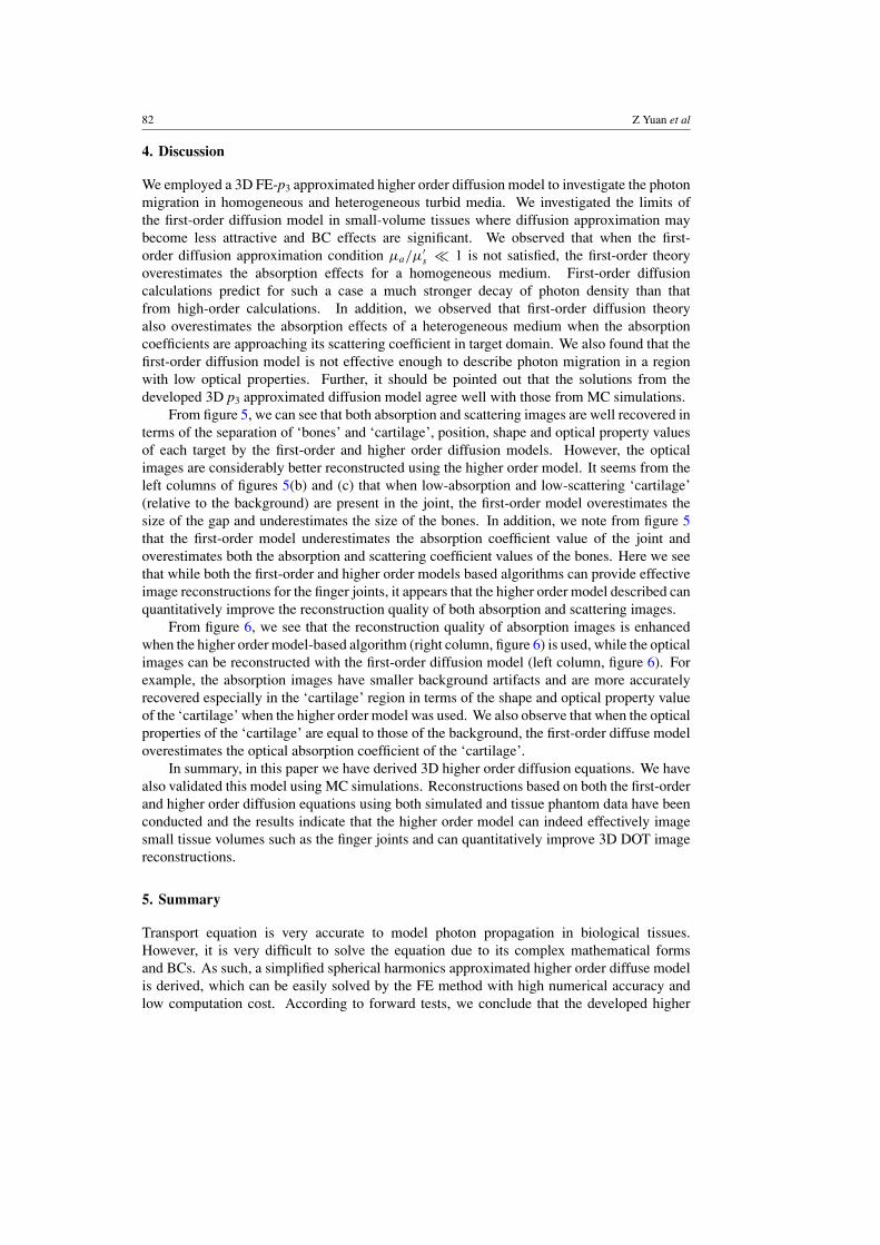
From figure 5, we can see that both absorption and scattering images are well recovered interms of the separation of ‘bones’ and ‘cartilage’, position, shape and optical property valuesof each target by the first-order and higher order diffusion models. However, the opticalimages are considerably better reconstructed using the higher order model. It seems from theleft columns of figures 5(b) and (c) that when low-absorption and low-scattering ‘cartilage’(relative to the background) are present in the joint, the first-order model overestimates thesize of the gap and underestimates the size of the bones. In addition, we note from figure 5that the first-order model underestimates the absorption coefficient value of the joint andoverestimates both the absorption and scattering coefficient values of the bones. Here we seethat while both the first-order and higher order models based algorithms can provide effectiveimage reconstructions for the finger joints, it appears that the higher order model described canquantitatively improve the reconstruction quality of both absorption and scattering images.

From figure 6, we see that the reconstruction quality of absorption images is enhancedwhen the higher order model-based algorithm (right column, figure 6) is used, while the opticalimages can be reconstructed with the first-order diffusion model (left column, figure 6). Forexample, the absorption images have smaller background artifacts and are more accuratelyrecovered especially in the ‘cartilage’ region in terms of the shape and optical property valueof the ‘cartilage’ when the higher order model was used. We also observe that when the opticalproperties of the ‘cartilage’ are equal to those of the background, the first-order diffuse modeloverestimates the optical absorption coefficient of the ‘cartilage’.

In summary, in this paper we have derived 3D higher order diffusion equations. We havealso validated this model using MC simulations. Reconstructions based on both the first-orderand higher order diffusion equations using both simulated and tissue phantom data have beenconducted and the results indicate that the higher order model can indeed effectively imagesmall tissue volumes such as the finger joints and can quantitatively improve 3D DOT imagereconstructions.

5. Summary

Transport equation is very accurate to model photon propagation in biological tissues.However, it is very difficult to solve the equation due to its complex mathematical formsand BCs. As such, a simplified spherical harmonics approximated higher order diffuse modelis derived, which can be easily solved by the FE method with high numerical accuracy andlow computation cost. According to forward tests, we conclude that the developed higher

A higher order diffusion model for three-dimensional photon migration 83

order diffusion model is able to accurately describe light propagation in biological tissuesand the solutions agree well with those from MC simulations. In addition, the developedmodel is also validated by inverse reconstruction computation in optical tomography. Usingimaging in small-volume tissues as an example, we observed significant differences betweenthe reconstructed results from the first-order and higher order diffusion equations.

Appendix

The moment equations derived from the p3 approximated RTE are written asl = 0, m = 0:

2∂ψ10

∂z+ 2

(∂ψ11

∂x+

∂γ11

∂y

)+ 2σ00ψ00 = s (A.1)

2∂γ10

∂z+ 2

(−∂ψ11

∂y+

∂γ11

∂x

)= 0 (A.2)

l = 1, m = 1:

6∂ψ21

∂z+ 2

∂ψ00

∂x− 2

∂ψ20

∂x+ 12

(∂ψ22

∂x+

∂γ22

∂y

)+ 6σ11ψ11 = 0 (A.3)

6∂γ21

∂z+ 2

∂ψ00

∂y− 2

∂ψ20

∂y+ 12

(−∂ψ22

∂y+

∂γ22

∂x

)+ 6σ11γ11 = 0 (A.4)

l = 1, m = 0:

2∂ψ00

∂z+ 4

∂ψ20

∂z+ 6

(∂ψ21

∂x+

∂γ21

∂y

)+ 6σ10ψ10 = 0 (A.5)

6

(−∂ψ21

∂y+

∂γ21

∂x

)= 0 (A.6)

l = 2, m = 1:

2∂ψ11

∂z+ 8

∂ψ31

∂z+ 2

∂ψ10

∂x− 2

∂ψ30

∂x+ 20

(∂ψ32

∂x+

∂γ32

∂y

)+ 10σ21ψ21 = 0 (A.7)

2∂γ11

∂z+ 8

∂γ31

∂z+ 2

∂ψ10

∂y− 2

∂ψ30

∂y+ 20

(−∂ψ32

∂y+

∂γ32

∂x

)+ 10σ21γ21 = 0 (A.8)

l = 2, m = 2:

10∂ψ32

∂z+

(∂ψ11

∂x− ∂γ11

∂y

)−

(∂ψ31

∂x− ∂γ31

∂y

)

+ 30

(∂ψ33

∂x+

∂γ33

∂y

)+ 10σ22ψ22 = 0 (A.9)

10∂γ32

∂z+

(∂ψ11

∂y+

∂γ11

∂x

)−

(∂ψ31

∂y+

∂γ31

∂x

)

+ 30

(−∂ψ33

∂y+

∂γ33

∂x

)+ 10σ22γ22 = 0 (A.10)

84 Z Yuan et al

l = 2, m = 0:

6∂ψ30

∂z+ 4

∂ψ10

∂z+ 12(

∂ψ31

∂x+

∂γ31

∂y) − 2

(∂ψ11

∂x+

∂γ11

∂y

)+ 10σ20ψ20 = 0 (A.11)

6∂γ30

∂z+ 4

∂γ10

∂z+ 12

(−∂ψ31

∂y+

∂γ31

∂x

)− 2

(−∂ψ11

∂y+

∂γ11

∂x

)+ 10σ20γ20 = 0 (A.12)

l = 3, m = 3:(∂ψ22

∂x− ∂γ22

∂y

)+ 14σ33ψ33 = 0 (A.13)

(∂ψ22

∂y+

∂γ22

∂x

)+ 14σ33γ33 = 0 (A.14)

l = 3, m = 1:

4∂ψ21

∂z+ 2

∂ψ20

∂x− 2

(∂ψ22

∂x+

∂γ22

∂y

)+ 14σ31ψ31 = 0 (A.15)

4∂γ21

∂z+ 2

∂ψ20

∂y− 2

(−∂ψ22

∂y+

∂γ22

∂x

)+ 14σ31γ31 = 0 (A.16)

l = 3, m = 2:

2∂ψ22

∂z+

(∂ψ21

∂x− ∂γ21

∂y

)+ 14σ32ψ32 = 0 (A.17)

2∂γ22

∂z+

(∂ψ21

∂y+

∂γ21

∂x

)+ 14σ32γ32 = 0 (A.18)

l = 3, m = 0:

6∂ψ20

∂z− 6

(∂ψ21

∂x+

∂γ21

∂y

)+ 14σ30ψ30 = 0. (A.19)

Taking the partial derivative of equation (A.3) with respect to x and equation (A.4) withrespect to y,

6∂2ψ21

∂z∂x+ 2

∂2ψ00

∂2x− 2

∂2ψ20

∂2x+ 12

(∂2ψ22

∂2x+

∂2γ22

∂y∂x

)+ 6σ11

∂ψ11

∂x= 0 (A.20)

6∂2γ21

∂z∂y+ 2

∂2ψ00

∂2y− 2

∂2ψ20

∂2y+ 12

(−∂2ψ22

∂2y+

∂2γ22

∂x∂y

)+ 6σ11

∂γ11

∂y= 0. (A.21)

Adding equations (A.20) and (A.21),

6∂2ψ21

∂z∂x+ 2

∂2ψ00

∂2x− 2

∂2ψ20

∂2x+ 12

(∂2ψ22

∂2x+

∂2γ22

∂y∂x

)+ 6σ11

(∂ψ11

∂x+

∂γ11

∂y

)

+ 6∂2γ21

∂z∂y+ 2

∂2ψ00

∂2y− 2

∂2ψ20

∂2y+ 12

(−∂2ψ22

∂2y+

∂2γ22

∂x∂y

)= 0 (A.22)

and then combining equation (A.1)

2

(∂ψ11

∂x+

∂γ11

∂y

)= s − 2σ00ψ00 − 2

∂ψ10

∂z(A.23)

A higher order diffusion model for three-dimensional photon migration 85

with equation (A.5),

2

(∂2ψ21

∂x∂z+

∂2γ21

∂y∂z

)+

2

3

∂2ψ00

∂2z+

4

3

∂2ψ20

∂2z+ 2σ10

∂ψ10

∂z= 0, (A.24)

we obtain

2

(∂ψ11

∂x+

∂γ11

∂y

)= s − 2σ00ψ00 +

1

σ10

(2

3

∂2ψ00

∂2z+

4

3

∂2ψ20

∂2z+ 2

(∂2ψ21

∂x∂z+

∂2γ21

∂y∂z

)).

(A.25)

On substituting equation (A.25) into equation (A.22) and assuming σ10 = σ11, we get

2

3

(∂2ψ00

∂2x+

∂2ψ00

∂2y+

∂2ψ00

∂2z

)+

(4

3

∂2ψ20

∂2z− 2

3

∂2ψ20

∂2x− 2

3

∂2ψ20

∂2y

)+ 4

(∂2ψ22

∂2x

)+ 4

∂2ψ21

∂z∂x

+ 4∂2γ21

∂z∂y+ 4

(−∂2ψ22

∂2y

)+ 8

∂2γ22

∂x∂y+ σ11(s − 2σ00ψ00) = 0. (A.26)

Equation (A.26) is our first governing equation for the 3D p3 approximation to RTE. Nowwe try to derive the other five governing equations below. We take the partial derivative ofequation (A.15) by x and equation (A.16) by y,

4∂2ψ21

∂z∂x+ 2

∂2ψ20

∂2x− 2

(∂2ψ22

∂2x+

∂2γ22

∂y∂x

)+ 14σ31

∂ψ31

∂x= 0 (A.27)

4∂2γ21

∂z∂y+ 2

∂2ψ20

∂2y− 2

(−∂2ψ22

∂2y+

∂2γ22

∂x∂y

)+ 14σ31

∂γ31

∂y= 0. (A.28)

Adding equations (A.27) and (A.28), we get

4∂2ψ21

∂z∂x+ 2

∂2ψ20

∂2x− 2

(∂2ψ22

∂2x+

∂2γ22

∂y∂x

)+ 14σ31

(∂ψ31

∂x+

∂γ31

∂y

)+ 4

∂2γ21

∂z∂y+ 2

∂2ψ20

∂2y

− 2

(−∂2ψ22

∂2y+

∂2γ22

∂x∂y

)= 0. (A.29)

Note that equation (A.11) can be written as

12

(∂ψ31

∂x+

∂γ31

∂y

)= 2

(∂ψ11

∂x+

∂γ11

∂y

)− 10σ20ψ20 − 4

∂ψ10

∂z− 6

∂ψ30

∂z. (A.30)

Also note that equation (A.22) can be further written as

− 1

6σ11

{6∂2ψ21

∂z∂x+ 2

∂2ψ00

∂2x− 2

∂2ψ20

∂2x+ 12

(∂2ψ22

∂2x+

∂2γ22

∂y∂x

)+ 6

∂2γ21

∂z∂y+ 2

∂2ψ00

∂2y− 2

∂2ψ20

∂2y

+ 12

(−∂2ψ22

∂2y+

∂2γ22

∂x∂y

)}=

(∂ψ11

∂x+

∂γ11

∂y

). (A.31)

We obtain the following equation after substituting equation (A.31) into equation (A.30):(∂ψ31

∂x+

∂γ31

∂y

)= −5

6σ20ψ20 − 1

36σ11

[6∂2ψ21

∂z∂x+ 2

∂2ψ00

∂2x− 2

∂2ψ20

∂2x+ 12

(∂2ψ22

∂2x+

∂2γ22

∂y∂x

)

+ 6∂2γ21

∂z∂y+ 2

∂2ψ00

∂2y− 2

∂2ψ20

∂2y+ 12

(−∂2ψ22

∂2y+

∂2γ22

∂x∂y

)]− 1

3

∂ψ10

∂z− 1

2

∂ψ30

∂z.

(A.32)

86 Z Yuan et al

Further, equation (A.5) can be rewritten as

1

6σ10

[2

(∂2ψ21

∂x∂z+

∂2γ21

∂y∂z

)+

2

3

∂2ψ00

∂2z+

4

3

∂2ψ20

∂2z

]= −1

3

∂ψ10

∂z. (A.33)

Equation (A.19) can be rewritten as

1

28σ30

[6∂2ψ20

∂2z− 6

(∂2ψ21

∂x∂z+

∂2γ21

∂y∂z

)]= −1

2

∂ψ30

∂z. (A.34)

Substituting equations (A.33) and (A.34) into equation (A.32),(∂ψ31

∂x+

∂γ31

∂y

)=

{−5

6σ20ψ20 − 1

36σ11

[6∂2ψ21

∂z∂x+ 2

∂2ψ00

∂2x− 2

∂2ψ20

∂2x+ 12

(∂2ψ22

∂2x+

∂2γ22

∂y∂x

)

+ 6∂2γ21

∂z∂y+ 2

∂2ψ00

∂2y− 2

∂2ψ20

∂2y+ 12

(−∂2ψ22

∂2y+

∂2γ22

∂x∂y

)]

+1

6σ10

[2

(∂2ψ21

∂x∂z+

∂2γ21

∂y∂z

)+

2

3

∂2ψ00

∂2z+

4

3

∂2ψ20

∂2z

]

+1

28σ30

[6∂2ψ20

∂2z− 6

(∂2ψ21

∂x∂z+

∂2γ21

∂y∂z

)]}(A.35)

and equation (A.35) into equation (A.29), we obtain

4∂2ψ21

∂z∂x+ 2

∂2ψ20

∂2x− 2

(∂2ψ22

∂2x+

∂2γ22

∂y∂x

)+ 14σ31

{−5

6σ20ψ20 − 1

36σ11

[6∂2ψ21

∂z∂x+ 2

∂2ψ00

∂2x

− 2∂2ψ20

∂2x+ 12

(∂2ψ22

∂2x+

∂2γ22

∂y∂x

)+ 6

∂2γ21

∂z∂y+ 2

∂2ψ00

∂2y− 2

∂2ψ20

∂2y

+ 12

(−∂2ψ22

∂2y+

∂2γ22

∂x∂y

)]+

1

6σ10

[2

(∂2ψ21

∂x∂z+

∂2γ21

∂y∂z

)+

2

3

∂2ψ00

∂2z+

4

3

∂2ψ20

∂2z

]

+1

28σ30

[6∂2ψ20

∂2z− 6

(∂2ψ21

∂x∂z+

∂2γ21

∂y∂z

)]}

+ 4∂2γ21

∂z∂y+ 2

∂2ψ20

∂2y− 2

(−∂2ψ22

∂2y+

∂2γ22

∂x∂y

)= 0. (A.36)

Equation (A.36) can be further written as

50

21

(∂2ψ20

∂2x+

∂2ψ20

∂2y

)+

4

3

(∂2ψ00

∂2z− 1

2

∂ψ200

∂2x− 1

2

∂ψ200

∂2y

)+

50

21

(∂2ψ20

∂2x+

∂ψ220

∂2y

)

+40

7

(∂2ψ22

∂2y− ∂2ψ22

∂x− 2

∂2γ22

∂x∂y

)− 10σ31σ20ψ20 +

110

21

∂2ψ20

∂2z

+20

7

(∂2ψ21

∂z∂x+

∂2γ21

∂z∂Y

)− 10σ 2

20ψ22 = 0. (A.37)

Equation (A.37) is the second governing equation for the 3D p3 approximation.Now we try to derive the third governing equation. From equation (A.9), we get

10∂ψ32

∂z+

(∂ψ11

∂x− ∂γ11

∂y

)−

(∂ψ31

∂x− ∂γ31

∂y

)+ 30

(∂ψ33

∂x+

∂γ33

∂y

)+ 10σ22ψ22 = 0.

(A.38)

A higher order diffusion model for three-dimensional photon migration 87

Based on equations (A.20) and (A.21), we get(∂ψ11

∂x− ∂γ11

∂y

)= 1

6σ11

{−

[6∂2ψ21

∂z∂x+ 2

∂2ψ00

∂2x− 2

∂2ψ20

∂2x+ 12

(∂2ψ22

∂2x+

∂2γ22

∂y∂x

)]

+

[6∂2γ21

∂z∂y+ 2

∂2ψ00

∂2y− 2

∂2ψ20

∂2y+ 12

(−∂2ψ22

∂2y+

∂2γ22

∂x∂y

)]}. (A.39)

From equations (A.15) and (A.16), we get

1

14σ31

{[4∂2ψ21

∂z∂x+ 2

∂2ψ20

∂2x− 2

(∂2ψ22

∂2x+

∂2γ22

∂y∂x

)]−

[4∂2γ21

∂z∂y+ 2

∂2ψ20

∂2y

− 2

(−∂2ψ22

∂2y+

∂2γ22

∂x∂y

)]}= −

(∂ψ31

∂x− ∂γ31

∂y

). (A.40)

Taking the partial derivative of equation (A.13) with respect to x and equation (A.14) withrespect to y, and then adding them gives(

∂ψ33

∂x+

∂γ33

∂y

)= 1

14σ33

[−

(∂2ψ22

∂2y+

∂2γ22

∂x∂y

)−

(∂2ψ22

∂2x− ∂2γ22

∂y∂x

)]. (A.41)

Substituting equations (A.9), (A.39)–(A.41) and taking the partial derivative of (A.17) withrespect to z in equation (A.38), we obtain

1

3

(∂2ψ00

∂2x− ∂2ψ00

∂2y

)− 10

21

(∂2ψ20

∂2x− ∂2ψ20

∂2y

)+

10

7

(∂2ψ21

∂x∂z− ∂2γ21

∂y∂z

)

+30

7

(∂ψ2

22

∂2x+

∂ψ222

∂2y+

1

3

∂2ψ22

∂2z

)− 10σ 2

00ψ22 = 0. (A.42)

This is the third governing equation for the 3D p3 approximation of RTE. Additionally,based on equations (A.3) and (A.4), we obtain

6∂2ψ21

∂z∂y+ 2

∂2ψ00

∂x∂y− 2

∂2ψ20

∂x∂y+ 12

(∂ψ2

22

∂x∂y+

∂2γ22

∂2y

)+ 6σ11

(∂ψ11

∂y+

∂γ11

∂x

)+ 6

∂2γ21

∂z∂x

+ 2∂2ψ00

∂y∂x− 2

∂2ψ20

∂y∂x+ 12

(−∂2ψ22

∂y∂x+

∂2γ22

∂2x

)= 0. (A.43)

From equations (A.15) and (A.16), we get

14σ31

(∂ψ31

∂y+

∂γ31

∂x

)= −

[4∂2γ21

∂z∂x+ 2

∂2ψ20

∂x∂y− 2

(−∂2ψ22

∂y∂x+

∂2γ22

∂2x

)]

−[

4∂2ψ21

∂z∂y+ 2

∂2ψ20

∂x∂y− 2

(∂2ψ22

∂x∂y+

∂2γ22

∂2y

)]. (A.44)

From equations (A.13) and (A.14), we get(∂2ψ22

∂y∂x+

∂2γ22

∂2x

)+ 14σ33

(∂γ33

∂x− ∂ψ33

∂y

)−

[(∂2ψ22

∂x∂y− ∂2γ22

∂2y

)]= 0. (A.45)

Note that equations (A.43)–(A.45) can be further written as

(∂ψ11

∂y+

∂γ11

∂x

)= − 1

6σ11

{[6∂2γ21

∂z∂x+ 2

∂2ψ00

∂y∂x− 2

∂2ψ20

∂y∂x+ 12

(−∂2ψ22

∂y∂x+

∂2γ22

∂2x

)]

+

[6∂2ψ21

∂z∂y+ 2

∂2ψ00

∂x∂y− 2

∂2ψ20

∂x∂y+ 12

(∂ψ2

22

∂x∂y+

∂2γ22

∂2y

)]}(A.46)

88 Z Yuan et al

−(

∂ψ31

∂y+

∂γ31

∂x

)= 1

14σ31

{[4∂2γ21

∂z∂x+

∂2ψ20

∂y∂x− 2

(−∂2ψ22

∂y∂x+

∂2γ22

∂2x

)]

+

[4∂2ψ21

∂z∂y+

∂2ψ20

∂x∂y− 2

(∂2ψ22

∂x∂y+

∂2γ22

∂2y

)]}(A.47)

30

(∂γ33

∂x− ∂ψ33

∂y

)= 15

7σ33

{[(∂2ψ22

∂x∂y− ∂2γ22

∂2y

)]−

[(∂2ψ22

∂y∂x+

∂2γ22

∂2x

)]}. (A.48)

When equations (A.46)–(A.48) and the partial derivative of (A.17) with respect to z

are substituted into equation (A.10), we obtain our fourth governing equation for the 3D p3

approximation:

2

3

∂2ψ00

∂x∂y− 20

21

∂2ψ20

∂x∂y+

30

7

(∂γ 2

22

∂2x+

∂γ 222

∂2y+

1

3

∂2γ22

∂2z

)

+10

7

(∂2ψ21

∂y∂z+

∂γ 221

∂x∂z

)− 10σ 2

00γ22 = 0. (A.49)

Moreover, from equations (A.7) and (A.3), we obtain

2∂ψ11

∂z+ 8

∂ψ31

∂z+ 2

∂ψ10

∂x− 2

∂ψ30

∂x+ 20

(∂ψ32

∂x+

∂γ32

∂y

)+ 10σ21ψ21 = 0

2∂ψ11

∂z= − 1

3σ11

[6∂ψ2

21

∂2z+ 2

∂2ψ00

∂x∂z− 2

∂2ψ20

∂x∂z+ 12

(∂2ψ22

∂x∂z+

∂2γ22

∂y∂z

)].

(A.50)

Based on equation (A.15), we get

8∂ψ31

∂z= − 4

7σ31

[4∂2ψ21

∂2z+ 2

∂2ψ20

∂x∂z− 2

(∂2ψ22

∂x∂z+

∂2γ22

∂y∂z

)]. (A.51)

From equation (A.19), we get

−2∂ψ30

∂x= 1

7σ30

[6

∂ψ220

∂z∂x− 6

(∂2ψ21

∂2x+

∂2γ21

∂y∂x

)]. (A.52)

Based on equations (A.17) and (A.18), we get

20

(∂ψ32

∂x+

∂γ32

∂y

)= − 10

7σ32

{[2∂2ψ22

∂z∂x+

(∂2ψ21

∂2x− ∂2γ21

∂y∂x

)]

+

[2∂2γ22

∂z∂y+

(∂2ψ21

∂2y+

∂2γ21

∂x∂y

)]}. (A.53)

From equation (A.5), we get

2∂ψ10

∂x= − 1

3σ10

[2∂2ψ00

∂z∂x+ 4

∂2ψ20

∂z∂x+ 6

(∂2ψ21

∂2x+

∂2γ21

∂y∂x

)]. (A.54)

As such, equation (A.7) is rewritten in consideration of equations (A.50)–(A.54):

4

3

∂2ψ00

∂x∂z+

20

21

∂2ψ20

∂x∂z+

30

7

(∂2ψ21

∂2z+

∂2ψ21

∂2x+

1

3

ψ221

∂2y

)

+40

7

(∂2ψ22

∂x∂z+

∂γ 222

∂y∂z+

1

2

∂2γ21

∂z∂y

)− 10σ 2

00ψ21 = 0. (A.55)

A higher order diffusion model for three-dimensional photon migration 89

This is the fifth governing equation for the 3D p3 approximation. When similarderivations are performed for equation (A.8), we get our final governing equation for the3D p3 approximated RTE,

4

3

∂2ψ00

∂y∂z+

20

21

∂2ψ20

∂y∂z+

30

7

(∂2γ21

∂2z+

1

3

∂2γ21

∂2x+

γ 221

∂2y

)

+40

7

(∂2γ22

∂x∂z− ∂ψ2

22

∂y∂z+

1

2

∂2ψ21

∂x∂y

)− 10σ 2

00γ21 = 0. (A.56)

References

Aronson R and Corngold N 1999 Photon diffusion coefficient in the absorbing medium J. Opt. Soc. Am. A 16 1066–71Aydin E, Olivera C R E de and Goddard A J H 2004 A finite element-spherical harmonics radiation transport model

for photon migration in turbid media J. Quant. Radiat. Spectrosc. Transfer 84 247–60Aydin E D, Oliveira C R E de and Goddard A J H 2002 A comparison between transport and diffusion calculations

using a finite element-spherical harmonics radiation transport method Med. Phys. 29 2013–23Barbour R L, Graber H L, Wang Y, Chang J H and Aronson R 1993 A perturbation approach for optical diffusion

tomography using continuous-wave and time-resolved data Proc. SPIE IS11 87–120Boas D A 1995 Photon migration within the P3 approximation Proc. SPIE 2389 240–47Boverman G, Fang Q, Carp S, Miller E, Brook D, Selb J, Moore R, Kopans D and Boas D A 2007 Spatio-

temporal imaging of the hemoglobin in the compressed breast with diffuse optical tomography Phys. Med. Biol.52 3619–41

Dehghani H, Delpy D and Arridge S 1999 Photon migration in non-scattering tissue and the effects on imagereconstruction Phys. Med. Biol. 44 2897–2906

Dorn A 1998 Transport—backtransport method for optical tomography Inverse Problems 14 1107–30Elaloufi R, Carminati R and Greffet J 2003 Definition of diffusion coefficient in scattering and absorbing media

J. Opt. Soc. Am A 20 678–85Golub Gene H and Loan Charles F Van 1996 Matrix Computation (Baltimore, MD: John Hopkins University Press)Hebden J, Arridge S and Delpy D 1997 Optical imaging in medicine: I. Experimental techniques Phys. Med. Biol.

42 825–40Hielscher A H, Alcouffe R E and Barbour R L 1998 Comparison of finite-difference transport and diffusion calculations

for photon migration in homogeneous and heterogeneous tissues Phys. Med. Biol. 43 1285–1302Iftimia N and Jiang H 2000 Quantitative optical image reconstruction of turbid media by use of direct-current

measurements Appl. Opt. 39 5256–61Jiang H 1999 Optical image reconstruction based on the third-order diffusion equations Opt. Express 4 241–6Jiang H, Paulsen K D, Osterberg U L, Pogue B W and Patterson M S 1996 Optical image reconstruction using

frequency-domain data: simulations and experiments J. Opt. Soc. Am A 13 253–66Jiang H, Xu Y and Iftimia N 2000 Experimental three-dimensional optical image reconstruction of heterogeneous

turbid media Opt. Express 7 204–9Jiang H, Xu Y, Iftimia N, Eggert J, Klove K, Barron L Lisa and Fajardo L 2001 Three-dimensional optical tomographic

imaging of breast in a human subject IEEE Trans. Med. Imag. 20 1334–40Kanmani B and Vasu R 2007 Noise-tolerance analysis for detection and reconstruction of absorbing inhomogeneities

with diffuse optical tomography using single- and phase-correlated dual-source schemes Phys. Med. Biol.52 1409–29

Klose A, Netz U, Beuthan J and Hielscher A H 2002 Optical tomography using the time-independent equation ofradiative transfer: Part 1. Forward model J. Quant. Radiat. Spectrosc. Transfer 72 691–713

Klose A D and Larson E W 2006 Light transport in biological tissue based on the simplified spherical harmonicsequations J. Comput. Phys. 220 441–70

Kim A and Ishimaru A 1998 Optical diffusion of continuous-wave, pilsed, and density waves in scattering media andcomparisons with radiative reansfer Appl. Opt. 37 5313–19

Paulsen K D and Jiang H 1995 Spatially-varying optical property reconstruction using a finite element diffusionequation approximation Med. Phys. 22 691–702

Oak Ridge National Laboratory 1990 RSIC Computer Code Collection ReportRui K, Bal G and Hielscher A H 2007 Transport and diffusion-based optical tomography in small volumes: a

comparative study Appl. Opt. 46 6669–79Song Z, Dong K, Hu X H and Lu J Q 1999 Monte Carlo simulations of converging laser beams propagation in

biological materials Appl. Opt. 38 2944–49

90 Z Yuan et al

Unlu M, Birgul O and Gulsen G 2008 A simulation study of the variability of indocyanine green kinetics andusing structural a priori information in dynamic contrast enhanced diffuse optical tomography Phys. Med. Biol.53 3189–3200

Xu M, Cai W, Lax M and Alfano R 2001 Photon transport forward model for imaging in turbid media Opt. Lett.26 1066–68

Yodh A and Chance B 1995 Spectroscopy and imaging with diffusing light Phys. Today 48 34–40Yuan Z and Jiang H 2007a Image reconstruction schemes that combines modified Newton method and efficient initial

guess estimate for optical tomography of finger joints Appl. Opt. 46 2757–68Yuan Z and Jiang H 2007b Three-dimensional finite-element-based photoacoustic tomography: reconstruction

algorithm and simulation Med. Phys. 34 538–46Yuan Z, Zhang Q, Sobel E and Jiang H 2007 3D diffuse optical tomography imaging of osteoarthritis: initial results

in finger joints J. Biomed. Opt. 12 034001Yuan Z, Zhang Q, Sobel E and Jiang H 2008 Tomographic x-ray-guided three-dimensional diffuse optical tomography

of osteoarthritis in the finger joints J. Biomed. Opt. 13 044006