A Hierarchical Ornstein–Uhlenbeck Model for Continuous Repeated Measurement Data

A HIERARCHICAL ORNSTEIN-UHLENBECK MODEL FOR

CONTINUOUS REPEATED MEASUREMENT DATA

Zita Oravecz, Francis Tuerlinckx, & Joachim Vandekerckhove

department of psychology, university of leuven

Oravecz, Z., Tuerlinckx, F., & Vandekerckhove, J. (in press). A hierarchical

Ornstein-Uhlenbeck model for continuous repeated measurement data. Psychometrika.

Correspondence and requests for reprints should be sent to Zita Oravecz, Research groupquantitative and personality psychology, Department of Psychology, University of Leuven,Tiensestraat 102, B-3000 Leuven, Belgium. E-Mail: [email protected]

an ornstein-uhlenbeck model 2

Abstract

In this paper, we present a diffusion model for the analysis of continuous-time

change in multivariate longitudinal data. The central idea is to model the data from

a single person with an Ornstein-Uhlenbeck diffusion process. We extend it

hierarchically by allowing the parameters of the diffusion process to vary randomly

over different persons. With this approach, both intra- and interindividual

differences are analyzed simultaneously. Furthermore, the individual difference

parameters can be regressed on covariates, thereby providing an explanation of

between-person differences. Unstructured and unbalanced data pose no problem for

the model to be applied. We demonstrate the method on data from an experience

sampling study to investigate changes in the core affect. It can be concluded that

different factors from the five factor model of personality are related to features of

the trajectories in the core affect space, such as the autocorrelation and variability

of the changes.

Key words: Ornstein-Uhlenbeck process, hierarchical, multivariate, Bayesian


1. Introduction

Change over time is a central and non-negligible concept that psychologists frequently

encounter while studying different phenomena such as learning processes, developmental

issues, or mood changes. Emotions and related phenomena are prime examples that are

subject to change over time, but also measures that are intuitively believed to be very stable

(such as personality characteristics (see e.g. Borkenau & Ostendorf, 1998)) reveal their

changing nature when repeated measures are taken. Going a step further, following the

arguments of van Montfort, Oud, and Satorra (2007), any serious causal analyses should be

based on longitudinal data.

Many longitudinal studies rely on panel designs: a large number of subjects with typically

fewer than 10 measurements per person. However, technical innovations such as palmtops,

beepers and online questionnaires have made it possible to measure variables of interest more

”intensively” than in the typical panel designs. Such intensive longitudinal designs (see Walls

& Schafer, 2006) have recently become quite popular. They typically consists of relatively long

(e.g., more than 50 measurement occasions) data chains from different subjects. Intensive

longitudinal data frequently stem from experience sampling techniques (Bolger, Davis, &

Rafaeli, 2003; Csikszentmihalyi & Larson, 1987; Larson & Csikszentmihalyi, 1983; Russell &

Feldman-Barrett, 1999), dyadic interaction studies (Ferrer & Nesselroade, 2003), or cognitive

and sensorimotor performance research (Li, Huxhold, & Schmiedek, 2004). These methods

often result in a highly unstructured longitudinal dataset, since the records may be taken at

different time points for different individuals. Moreover, missing data often occur, which leads

to unequal numbers of observations.

Apart from a few exceptions (e.g., Oud & Singer, 2008; Singer, 2008), time is generally

handled in a discrete way in longitudinal models. This property makes modeling such data

somewhat unrealistic, since the measured phenomena do not cease to exist between

observations. Oud (2002) argues that most processes in behavioral sciences unfold in

continuous time and should be handled accordingly. Treating a theoretically continuous

variable as discrete may lead to biased results, for a discussion see Delsing, Oud, and Bruyn

(2005). In contrast, continuous-time modeling appears to be a more realistic solution.

In this paper, we focus on introducing a hierarchical model for analyzing intensively

measured variables while allowing for change in continuous time. This way, intra- and


interindividual differences are studied simultaneously. The model incorporates two distinctive

properties. First of all, it concentrates on the dynamic feature of the change process by

investigating a mean-reverting tendency over time. Second, it explores interindividual

variability from different perspectives, some of which have not been considered so far. Both

aspects are summarized below.

Concerning the first special property, the paper introduces a stochastic process with

Markovian properties, namely the Ornstein-Uhlenbeck (OU) process, to serve as the basic

model for change within an individual. The OU process can be seen as a mathematical model

of temporal change for phenomena with regulatory, mean-reverting, or centralizing

mechanisms. This property makes the process especially useful for modeling moods and

emotions (Larsen, 2000; Lykken & Tellegen, 1996), but it can also be applied to other change

processes with a possible regulatory mechanism (e.g., balance control). When we use the OU

process as an analytical tool, the focus is more on the dynamics of the process, and not so

much on the systematic or structural changes with respect to the mean level, as is commonly

investigated by mixed models (e.g., Diggle, Heagerty, Liang, & Zeger, 2002; Verbeke &

Molenberghs, 2000). This way, our approach is closer to the area of time series analysis, but a

distinctive aspect is that our main emphasis lies on studying interindividual differences in

temporal change, while time series analysis mainly focuses on a single measurement chain.

Regarding the second characteristic, the proposed hierarchical model is suited for

exploring interindividual differences from aspects which have been neglected so far. Other

existing techniques, like structural equation modeling (SEM, Bollen, 1989), multilevel

modeling (Goldstein, 2003; Raudenbush & Bryk, 2002), state-space modeling either combined

with SEM or with Kalman filter estimation procedure (Oud, 2007; Oud & Singer, 2008) do

not commonly deal with interindividual differences with respect to all model parameters. In

the hierarchical model presented here, parameters like the serial- or the cross-correlation are

considered to be person-specific, and in this way we allow new aspects of interindividual

differences to be investigated.

Regarding statistical inference, we will make use of a Bayesian approach (Gelman, Carlin,

Stern, & Rubin, 2004). The Bayesian methodology offers a sound way for statistical inference

in models with a complex hierarchical structure. With respect to the present model, since all

the OU parameters can be turned into random effects and can be regressed onto predictors or


covariates (De Boeck & Wilson, 2004), the parameter estimation in the classical framework

would involve a high-dimensional integration over the numerous random effect distributions.

In contrast, the paper will demonstrate that the hierarchical OU model can be fitted in a

straightforward way using the Bayesian framework. Also, the most commonly used statistical

inference technique in continuous time modeling involves some approximation methods to

estimate the parameters, while with the Bayesian approach this is no longer necessary.

The OU process in particular and some variants of it (e.g., the integrated OU process)

have been proposed as models for the analysis of longitudinal profiles in several fields. For

example, single time series from measurements of animal movement have been modeled as an

OU process by Blackwell (1997, 2003), Brillinger, Preisler, Ager, and Kie (2004) and Dunn

and Gipson (1977). A major difference between our psychological approach and this biological

application is that in the latter there is no interest in describing and explaining differences

between subjects. In the context of mixed models for longitudinal data analysis, the

integrated OU process is proposed to model serial correlation between measurements (e.g., see

Cruz-Mesıa & Marshall, 2006; Sy, Taylor, & Cumberland, 1997; Taylor, Cumberland, & Sy,

1994) but no interindividual variation is allowed in the driving parameters of the process.

The structure for the remainder of the article is as follows. In the next section, we explain

the OU diffusion process together with the interpretation of its parameters. Subsequently, we

discuss a hierarchical extension. The following section summarizes the statistical inference and

afterwards an application to the modeling of core affect trajectories is presented. The last part

presents our conclusion.

2. The theory of the Ornstein-Uhlenbeck diffusion process

In this section, we give a non-technical and self-contained account of the OU diffusion

process. More detailed explanations can be found in Cox and Miller (1972), Dunn and Gipson

(1977), Karlin and Taylor (1981), and Blackwell (2003). Usually, the model is presented as a

solution to a first-order stochastic differential equation (SDE). However, since the details of

the SDE may not be generally known, we will start with the solution and introduce the SDE

only later. At this point, we do not yet present an application, so our explanation will be in

general terms without reference to a substantive area.

Let us assume that the state of an individual at time t (t ≥ 0) can be represented as a


point Y (t) = (Y1(t), Y2(t), ..., Yq(t))T in a continuous, q-dimensional space. In general, an OU

diffusion process is a continuous-time Gaussian process Y (t) : t ≥ 0 defined on this

q-dimensional space such that, given that the process was in state Y (t) at time t, the

conditional distribution of the position Y (t + d) d time units later is:

Y (t + d) | Y (t) ∼ Nq(µ + e−Bd(Y (t) − µ), Γ − e−BdΓe−B′d) (1)

where µ is a q-dimensional vector and B and Γ are q × q matrices. The function eM (with M

a square matrix) is the matrix exponential. The matrix exponential eM is defined as follows:

eM = I +

∞∑

j=1

M j

j!.

As a special case (see later), if M is a diagonal matrix with diagonal elements m1, ...,mq, it is

equal to:

eM =

em1 . . . 0...

. . ....

0 . . . emq

where emi is the scalar exponential function value of mi.

If B is a positive definite matrix (and if E(Y (0)) = µ and var(Y (0)) = Γ), then the

Ornstein-Uhlenbeck process is stationary. This can be seen intuitively by letting d → ∞, so

that the matrix exponential part e−Bd goes to zero and the process has the following

equilibrium or stationary distribution:

Y (t) ∼ Nq(µ,Γ). (2)

From Equation (2), it can be deduced that µ is the mean of the equilibrium distribution and

Γ is its covariance matrix (hence, Γ is positive definite). The assumption of stationarity

implies that if the process runs for an infinitely long period of time, this equilibrium density is

the density function of the visited points in the q-dimensional space. It will also be assumed in

this paper that the distribution of Y (0) (the first measurement, when time t equals 0) is the

equilibrium distribution (in which case the model is strictly stationary).

To explain the interpretation of the distinct parameter vectors and matrices in the model,

it is best to start by examining the conditional mean vector µ + e−Bd(Y (t) − µ) from

Equation (1). It can be seen that this conditional mean depends on the previous position


Y (t), on the time difference d between the two measurements and on the µ and B parameters

of the process. The interpretation of µ and B is the following: The parameter µ is the vector

of expected values of the equilibrium distribution (let d → ∞) and can thus be seen as a fixed

point attractor in the q-dimensional space. Because of this property, µ can be called the

average position or the ”homebase” of the process. The other parameter, the matrix B

controls the strength of the centralizing tendency, which keeps the process in the vicinity of

the homebase. This matrix represents a mean reverting or dampening force, since it impedes

the process to diffuse away from the homebase. To illustrate the role of the centralizing

tendency, it is easier to see its function in a one-dimensional model (i.e., q = 1). In that case,

the conditional mean of Y (t + d) given Y (t) is equal to µ + e−βd(Y (t) − µ) (with, as required,

β > 0). From the latter equation, it can be easily derived that (1) if β is large, the conditional

mean is very close to the homebase and (2) if β approaches zero, the homebase takes a value

close to the previous position.

To simplify the interpretation in the general q-dimensional case, in this paper we only

deal with the subset of isotropic B matrices, that is B = βI, where I is the q × q identity

matrix. The isotropic restriction is motivated by two main reasons. The first is a pragmatic

one since making the matrix B isotropic reduces the complexity of the model substantially. It

is not unusual in the applied literature on the OU process to use such a constraint (see e.g.,

Blackwell, 2003). For a general B, not only does just B have to be positive definite but the

matrix BΓ + ΓB′ as well (Dunn & Gipson, 1977). Satisfying this constraint in the estimation

process is quite cumbersome. A second and more substantive reason to prefer the isotropic

parametrization is that it does not give any special importance to the chosen coordinate

system. If the matrix B is isotropic, the expected trajectories near the homebase are straight

lines and therefore the centralizing tendency matrix is invariant under rotation and reflection

(see also Blackwell, 1997). Accordingly, the centralizing tendency is controlled only by the

distance from the homebase of the process and not by its direction. However, for non-isotropic

centralizing tendency matrices, the expected trajectories close to the homebase are generally

not straight lines, but are curved. In the latter case, special importance is given to the

coordinate system at hand. However, in most psychological applications, the coordinate

system is arbitrary (see also the application below).

If B is restricted to be isotropic, then it holds that e−Bd = e−βdI. Hence, if β is large (in


which case there is a strong centralizing tendency), the exponential factor in the conditional

mean µ + e−βd(Y (t) − µ) goes to 0, so that the next point is a draw from a normal

distribution with the homebase µ as a mean. Alternatively, if β is small (i.e., weak centralizing

tendency), the exponential factor is close to 1 and the next position is a draw from a normal

distribution with the previous position as its mean. Thus, as in the one-dimensional case, the

matrix exponential e−Bd part behaves as a weighting function, taking values between 0 and 1,

and adding a certain proportion to the homebase from the distance between the previous

point and the homebase. For isotropic B matrices, it holds that the conditional mean lies

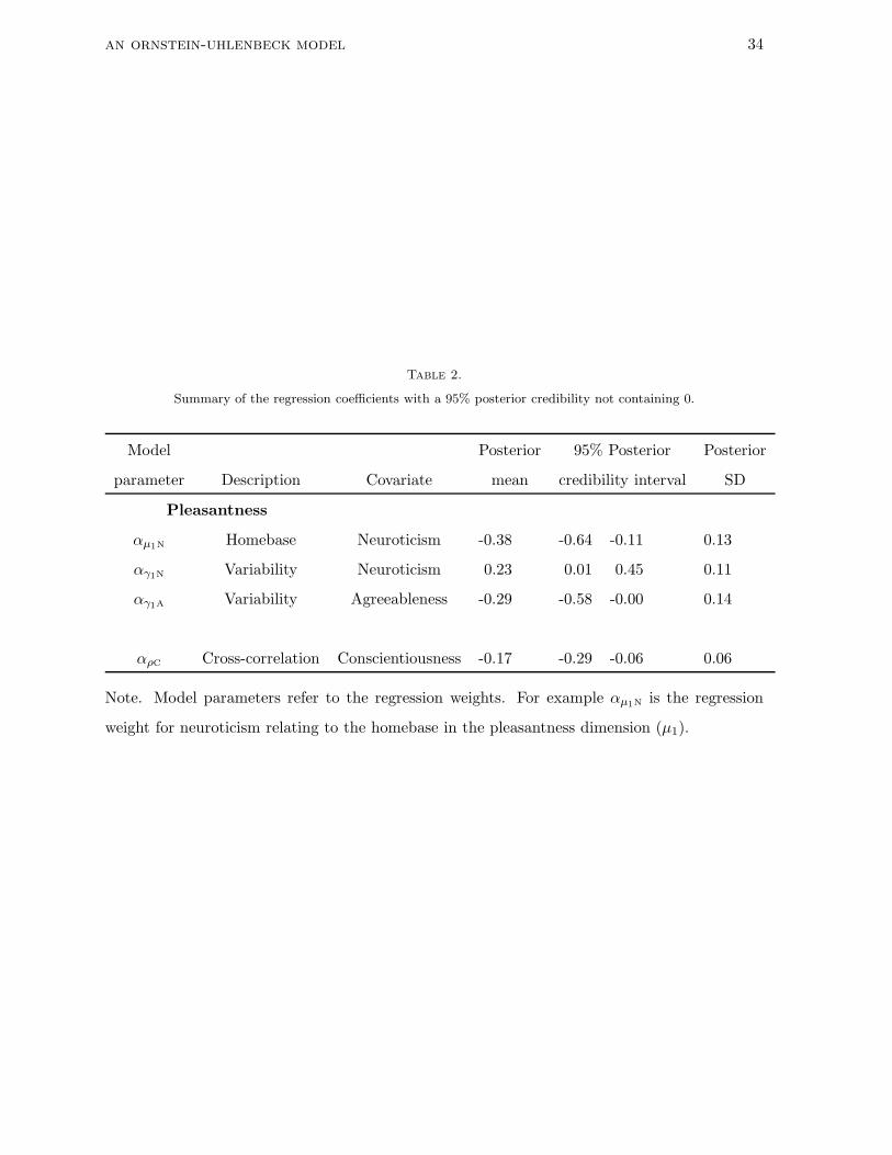
somewhere on the straight line connecting µ and Y (t). This is further illustrated in Figure 1

where the 0.5 probability contour curves of three conditional distributions from Equation (1)

for a two-dimensional (q = 2) model are drawn. A cross × denotes the center of each

conditional distribution. In all three cases, all parameters are kept constant, except for the

centralizing tendency which can take a small, medium, or large value (see the figure for the

exact numerical values). With a small β value, the conditional mean of the distribution of the

next point is close to the previous point but as β increases the conditional mean is moving

closer to the homebase. Note that the conditional variance also depends on the centralizing

tendency parameter: a larger β value implies a larger variability (see later).

=========================

Insert Figure 1 about here

=========================

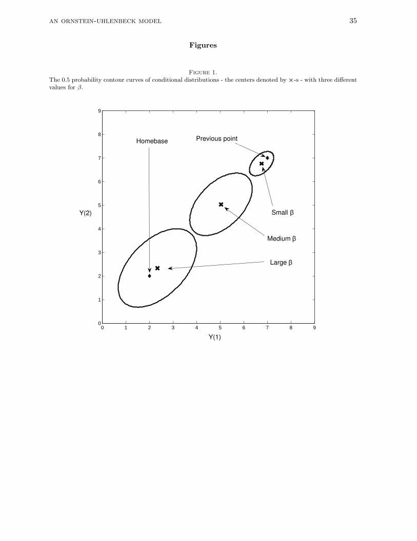
The centralizing tendency controls the autocorrelation function. In Appendix A it is

shown that the (continuous) autocorrelation function ρ(d) of an OU process equals e−βd.

Because the autocorrelation function is an exponentially decaying function of (continuous)

time, the OU process is the continuous time variant of an autoregressive process of order 1.

Brockwell and Davis (2002) denote such a process as a CAR(1) process (where C stands for

continuous-time). Figure 2 shows the change in the autocorrelation function as a function of

time for four different β values. Although the range of the β parameter is relatively small, it

has a remarkable effect on the slope of the autocorrelation function. Large (small) β values

lead in general to small (large) autocorrelation because the serial correlation function decays

more (less) steeply.


=========================


=========================

The matrix Γ is the covariance matrix of the stationary distribution in Equation (2) and

is part of the conditional covariance. It is a positive definite, symmetric q × q matrix

containing the variances for each dimension on the diagonal (denoted with the corresponding

row index) and the covariances as off-diagonal elements:

Γ =

γ1 . . . γ1q

.... . .

...

γq1 . . . γq

.

Large variance values imply that the process can go through many changes (i.e., it is very

volatile), while small variances lead to smoother trajectories. The covariances represent the

extent to which changes in one dimension tend to covary with changes in another dimension.

In a unidimensional context, the single γ parameter is often referred to as the volatility

parameter.

Examining the features of the instantaneous variance Γ − e−BdΓe−B′d, we can see that as

the exponential part goes to 0 (i.e., a large centralizing tendency and/or time difference), the

instantaneous variance converges to the variance of the stationary distribution. As the

exponential part goes to 1 (i.e., small centralizing tendency and/or time difference), the

conditional variance becomes very small. To illustrate this, assume for simplicity that q = 2

(and B is isotropic). Then Γ − e−BdΓe−B′d equals:

γ1(1 − e−2βd) γ12(1 − e−2βd)

γ12(1 − e−2βd) γ2(1 − e−2βd)

from which we can see the effect of the centralizing tendency β for a higher dimensional case

(given a constant time difference). On the one hand, when β is large, γ1 and γ2 are multiplied

by a number close to one and hence the instantaneous variances are near to the variances of

the stationary distribution. On the other hand, when β is small, the conditional variances are

close to 0. The same reasoning applies to the covariances. However, when considering the

instantaneous cross-correlations, it can easily be seen that they are independent of the


centralizing tendency and the time difference. Moreover, they are equal to the correlations of

the stationary distribution (ρ = γ12√γ1

√γ2

).

As already mentioned above, Equation (1) is part of the solution of a stochastic

differential equation (SDE). Without presenting too much technical detail, the SDE is a

convenient and intuitively appealing way of representing the OU process because it provides a

link with the more familiar field of deterministic differential equations. A full and rigorous

treatment of SDEs can be found in Arnold (1974), Karlin and Taylor (1981) and Smith (2000).

For demonstrative purposes, we simplify matters here, and we will assume that q = 1, such

that the vector µ and the matrices Γ and B reduce to the scalars µ, γ and β, respectively. For

the one-dimensional OU process as considered in this paper, the corresponding SDE equals

dY (t) = β(µ − Y (t))dt +√

2βγdW (t), (3)

where dY (t) is the (random) change in the process Y (t) in a small time interval (t, t + dt) and

W (t) represents a univariate standard (i.e., driftless and variance equal to one) Wiener

process, which is a mathematical model for a continuous-state continuous-time process with

independent increments (i.e., Brownian motion). The quantity dW (t) is the increment of this

process W in the small time interval (t, t + dt). As can be seen from Equation (3), the change

in Y (t) consists of two components: a deterministic part and a stochastic part (embodied by

the Wiener process term). The solution of such a SDE requires a special stochastic calculus

which we will not further discuss here (a short introduction can be found in Brockwell &

Davis, 2002).

However, if we let γ → 0, so that the stochastic part disappears, we are left with a simple

first-order linear differential equation. One can also see that the magnitude of change in the

deterministic part depends on the difference between the homebase µ and the current position

Y (t). If there were no stochastic disturbance in Equation (3), the solution of the deterministic

differential equation (given an arbitrary initial value at time 0 of Y (0)) would be equal to:

Y (t) = µ + (Y (0) − µ)e−βt.

This solution represents the scalar version of the mean of the conditional distribution in

Equation (1). Given the initial value Y (0), the exact position of the deterministic process can

be found for every time difference t. Moreover, if the time difference becomes large, the


process converges to the homebase µ. However, when the stochastic disturbance term is added

again, the OU process is retrieved and the exact position of the process is unpredictable

because of the inherent stochastic nature of the process.

In the following section, we will discuss how to extend the basic OU process in order to

make it appropriate for studying interindividual differences.

3. Hierarchical extension of the OU process

For the case where longitudinal data are collected for a random sample of persons, as is

often the case in psychological research, it is natural to consider a hierarchical extension of the

OU diffusion process in order to describe and explain interindividual differences. A hallmark

of the presented model is that all parameters are allowed to vary over individuals (and not

only the means as is commonly done).

Let us first fix some notation. A specific person p (p = 1, ..., P ) is measured np times at

the following sequence of time points: tp1, tp2, . . . , tps, . . . , tp,np . Note that we do not require

that persons are measured at regular time intervals or that they are measured at exactly the

same time points. The measured sequence of positions in the multidimensional space is

denoted as Y (tp1), ...,Y (tps), ...,Y (tp,np). (Note that we will usually set tp1 equal to 0 for all

persons to align the measurements of the different persons.) For all persons, the model for the

first observation of the chain of measurements is the person-specific equilibrium distribution:

Y (tp1) ∼ Nq(µp,Γp). (4)

This assumption can be justified, since in many applications the process has been diffusing

long enough to have converged to its stationary distribution and forgotten its initial position.

For the subsequent points, we rely on Equation (1) the conditional distribution of a single

person p at time ts given its position at the previous measurement occasion Y (tp,s−1) is

normal with conditional mean vector δps and conditional covariance matrix Λps

Y (tps) | Y (tp,s−1) ∼ Nq(δps,Λps) (5)

where

δps = µp + e−Bp(tps−tp,s−1)(Y (tp,s−1) − µp)

and

Λps = Γp − e−Bp(tps−tp,s−1)Γpe−B

′

p(tps−tp,s−1).


Note that all parameter vectors and matrices carry an index p to denote that they are allowed

to be person specific.

In a hierarchical model, the individual parameters are assumed to be drawn from a

population distribution. Instead of merely listing the distributions the different parameter

vectors and matrices can follow, we will also directly indicate how person-specific covariate

information can be included in order to explain interindividual differences in the basic OU

parameters. If one only wants to describe the amount of between-person variation in some

parameters, the covariates can be removed from the model so that only the intercept is left.

Let us suppose that k covariates are measured and xjp denotes the score of person p on

covariate j (j = 1, ..., k). Then we can collect all covariate scores into a vector (together with a

constant 1 for the intercept) x′p = (1, x1p, x2p, ..., xkp). Furthermore, let αµ1 be the vector (of

length k + 1) with regression coefficients for the regression of the individual homebases onto

the covariates. The vectors with regression coefficients for the other parameters are given

names in a similar fashion (e.g., αβ for β, etc.).

At this point, we will introduce a simplification of our model in order to make the

exposition not overly complex. Most potential applications we encountered for the hierarchical

OU model are two-dimensional in nature and therefore we will assume in the remainder of the

paper that q = 2. However, the extension to higher-dimensional cases is mostly evident,

except for one part of the model (the variances) but it will be indicated explicitly how the

general case can be handled.

The person-specific homebase µp (for q = 2) is assumed to be a draw from the following

bivariate normal distribution:

µp ∼ N2

(

αµx′p,Σµ

)

, (6)

where

αµ = (αµ1 ,αµ2),

so that αµ is a (k + 1) × 2 matrix of regression coefficients. Furthermore, the matrix Σµ,

which is defined as:

Σµ =

σ2µ1

σµ1µ2

σµ1µ2 σ2µ2

,

is the (residual) covariance matrix, representing the variations and associations that exist in

the population between the individual means of the stationary distribution after taking into


account the person covariates. As said above, if only the intercept is present in the covariate

vector, then the model just describes the population mean vector of the homebases and the

variability in the population. Note that the regression of µp onto covariates is in general a

q-variate multiple regression problem since µp is of length q.

Not only the mean of the stationary distribution is assumed to be person-specific but its

covariance matrix as well:

Γp =

γ1p γ12p

γ12p γ2p

.

We need to propose a population distribution for these covariance matrices such that positive

definiteness of Γp is ensured. Moreover, we would like to regress the variances and covariances

on covariates. An obvious choice would be to assume that Γp is a draw from an

inverse-Wishart distribution. However, such a distribution does not allow the regression of

variances and covariances on covariates in a natural way. One possible alternative is to

decompose the covariance matrix (Barnard, McCulloch, & Meng, 2000), usually into standard

deviations and correlation matrices and assume proper distributions for these in order to

ensure the positive definiteness. In this paper, we make use of the fact that Γp is a two-by-two

covariance matrix such that it can be decomposed into two variances and a correlation. Next,

the logarithms of the variances are assumed to be sampled from a normal distribution. After

applying the Fisher-z transformation to the correlation coefficient, the transformed value is

taken as a draw from a normal distribution, which also provides the possibility of regressing

the mean of this distribution on covariates.

The two diagonal elements of the covariance matrix Γp are regressed on the covariates in

the following way:

log(γ1p) ∼ N(x′pαγ1 , σ

2γ1

)

log(γ2p) ∼ N(x′pαγ2 , σ

2γ2

),

with αγ1 and αγ2 being regression coefficient vectors with k + 1 components. Since it is

assumed that the log-transformed γ-parameters are normally distributed, the original

γ-parameters follow a lognormal distribution:

f(γup) =1

γup

√

2πσ2γu

e− 1

2

(log(γup)−x′

pαγu )2

σ2γu , (7)


for u = 1, 2 and where f(·) will be used in the remainder of the paper as the generic symbol to

denote a probability density function.

The covariance parameter γ12p of Γp can be expressed in terms of standard deviations

and the correlation: γ12p =√

γ1p ×√γ2p × ρp. Instead of proposing a population distribution

for the covariance parameter, it will be assumed that the Fisher-z transformed (or

z-transformed for short) individual-specific cross-correlation coefficient F (ρp) is drawn from a

normal population distribution whose mean depends on covariates

F (ρp) ∼ N(x′pαρ, σ

2ρ).

The parameter ρp is the cross-correlation for a person p and it indicates the extent to which

changes in one dimension tend to correlate with changes in the other dimensions for person p.

From the mean of the population distribution of the z-transformed ρp, it can be learned

whether there is on average (i.e., in the population) a positive, negative, or zero correlation

between the changes in two dimensions. The density of the original ρp then equals (applying

the transformation of variables technique, see e.g., Mood, Graybill, & Boes, 1974):

f(ρp) =

∣

∣

∣

∣

dF (ρp)

dρp

∣

∣

∣

∣

φ(F (ρp);x′pαρ, σ

2ρ)

=1

(1 − ρp)(1 + ρp)

1√

2πσ2ρ

exp

(

− 1

2

(

12 log

(1+ρp

1−ρp

)

− x′pαρ

)2

σ2ρ

)

, (8)

where F (·) is the Fisher-z transform and φ(x;µ, σ2) is the normal density evaluated at x with

mean µ and variance σ2. Again, αρ contains k + 1 regression coefficients.

It should be noted that the solution outlined here, where the elements of the matrix Γp

are regressed onto covariates while still maintaining the positive definiteness of Γp, is only

valid in the two-dimensional case. For q > 2 and with a regression of the elements of the

covariance matrix on predictors, we refer to Daniels and Pourahmadi (2002), whose approach

is based on a Cholesky decomposition of the covariance matrix Γp.

Finally, because the centralizing tendency matrix Bp is isotropic, we need to assume a

population distribution only for the single parameter βp. Since βp has to be positive, similarly

to the variance parameters, it is assumed that the log-transformed βp-values follow a normal

distribution whose mean again depends on the covariates:

log(βp) ∼ N(x′pαβ , σ2

β),


where the length of vector αβ is k + 1. As in the case of the variance parameters (γ1p and

γ2p), the distribution of βp is lognormal:

f(βp) =1

βp

√

2πσ2β

e− 1

2

(log(βp)−x′

pαβ)2

σ2β . (9)

This completes the description of the model and puts us in a position to address issues of

statistical inference.

4. Statistical inference for the Ornstein-Uhlenbeck model

The intrinsic complexity of the model motivated us to perform all statistical inferences in

a Bayesian framework. The model complexity is mainly the result of the fact that all

parameters are treated in a hierarchical sense and are allowed to differ over persons. The

resulting high-dimensional integration over the many random effects distributions cannot be

handled using brute force quadrature methods. Therefore, parameter estimation is done by

sampling from the posterior density using a MCMC algorithm. For the model selection we

rely on the Deviance Information Criterion (DIC; Spiegelhalter, Best, Carlin, & Linde, 2002).

The major part of this section is devoted to the estimation of the parameters. More details

about the Bayesian methodology can be found in Gelman et al. (2004) and Robert and

Casella (2004).

As a first step, we derive the likelihood. Let us denote the data from person p as follows:

Y (tps)np

s=1. Given the sequence of observations from person p, the likelihood contribution for

person p reads as:

f(Y (tp1) | µp,Bp,Γp)

np∏

s=2

f(Y (tps) | Y (tp,s−1),µp,Bp,Γp)

∝np∏

s=1

|V ps|−12 e−

12

(

λTpsV −1

ps λps

)

(10)

with

λps =

Y p1 − µp if s = 1

Y ps −[

µp + e−Bp(tps−tp,s−1)(Y (tp,s−1) − µp)]

if s > 1

V ps =

Γp if s = 1

Γp − e−Bp(tps−tp,s−1)Γpe−B

′

p(tps−tp,s−1) if s > 1.(11)


The likelihood of all person-specific parameters (given the data from all persons 1, . . . , P and

making use of the fact that the persons are independent) then equals

f(Y (t1s)n1s=1, . . . , Y (tPs)nP

s=1 | µ1, . . . ,µP ,B1, . . . ,BP ,Γ1, . . . ,ΓP )

=P∏

p=1

f(Y (tps)np

s=1 | µp,Bp,Γp) ∝P∏

p=1

np∏

s=1

|V ps|−12 e−

12

(

λTpsV −1

ps λps

)

, (12)

where λps and V ps are defined as in Equation (11).

To find the posterior distribution, let us first collect (for simplicity) all model parameters

in a single parameter vector θ which contains the (unique) elements of the person-specific

vectors and matrices µ1, . . . ,µP ,Γ1, . . . ,ΓP ,B1, . . . ,BP , the regression coefficients

αµ,αγ1 ,αγ2 ,αρ,αβ , the residual (co)variances Σµ, σ2γ1

, σ2γ2

, σ2ρ, σ

2β. The joint posterior of all

parameters can then be written as follows:

f(θ | Y (t1s)n1s=1, . . . , Y (tPs)nP

s=1)

∝ f(Y (t1s)n1s=1, . . . , Y (tPs)nP

s=1 | µ1, . . . ,µP ,B1, . . . ,BP ,Γ1, . . . ,ΓP )

×P∏

p=1

f(µp | αµ,Σµ) ×P∏

p=1

2∏

u=1

f(γup | αγu , σ2γu

) ×P∏

p=1

f(ρp | αρ, σ2ρ) ×

P∏

p=1

f(βp | αβ, σ2β)

×f(αµ)f(αγ1)f(αγ2)f(αρ)f(αβ)f(Σµ)f(σ2γ1

)f(σ2γ2

)f(σ2ρ)f(σ2

β), (13)

where we have assumed independence between all sets of prior parameters. The distributions

of the person-specific parameters (third line of Equation (13)) are given in

Equations (6), (7), (8) and (9).

In Equation (13) we have not yet specified the prior distributions (last line of the

equation). For all regression coefficients α we assume a uniform prior:

f(αg) ∝ 1,

where g can be equal to µ1, µ2, γ1, γ2, ρ or β (for the two-dimensional case). The prior

distribution of Σµ is assumed to be equal to:

f(Σµ) ∝| Σµ |−(q+1)/2

which is Jeffreys prior, and q = 2 in the two-dimensional case. We choose noninformative

priors for all the other variance parameters σ2g as well:

f(σ2g) ∝ σ−2

g


which is a uniform prior on log σ. For the two-dimensional case g can be equal to µ1, µ2,

γ1,γ2, ρ or β.

To sample from the joint posterior, we make use of the Gibbs sampler (Gelman et al.,

2004, Robert & Casella, 2004). For this, we need to derive the full conditionals, that is, the

conditional distribution of each parameter given the other parameters and the data. In many

cases, the full conditionals are known densities from which one can sample directly. If the full

conditional is an unknown distribution, we make use of a Metropolis-Hastings step in the

Gibbs sampler to obtain a draw from it. Because of reasons of efficiency, when deriving the

full conditionals, we try to treat parameters that logically belong together as one block (e.g.,

Σµ or αµ1). We start with the full conditionals of the regression coefficients for the variances,

the centralizing tendency and the cross-correlation and subsequently treat the residual

variances of these parameters. Next, we treat the regression coefficients and residual

covariance matrix for the mean positions and move then to the lowest level parameters (the

individual homebases, variances, cross-correlations and centralizing tendencies).

With regard to the unidimensional parameters (γ1, γ2, ρ, and β), the full conditionals of

their regression coefficients (αγ1 , αγ2 , αρ, and αβ) and their residual variances (σ2γ1

, σ2γ2

, σ2ρ,

and σ2β) can be derived in a similar fashion. Here we give the example of the full conditional of

αγ1 and σ2γ1

, but γ1 could be substituted by γ2, ρ, or β as well. The full conditional of αγ1

reads as:

f(αγ1 | γ11, . . . , γ1P , σ2γ1

) ∝ |V g|−12 exp

(

− 1

2(αγ1 − Xαγ1)

′ V −1g (αγ1 − Xαγ1)

)

, (14)

where X is a P × (k + 1) matrix defined by stacking the person-specific covariate vectors x′p

below each other. If we denote g = (log(γ11), . . . , log(γ1P ))′ such that αγ1 = (X ′X)−1X ′g

and V g = σ2γ1

(X ′X)−1, it can be seen that the full conditional of αγ1 is a normal density with

mean Xαγ1 and covariance matrix V g.

The full conditional for σ2γ1

, the residual variance of αγ1 , follows a scaled inverse-χ2

distribution:

f(σ2γ1

| γ11, . . . , γ1P ) ∝ (σ2γ1

)−(

P−k−12

+1)

e− (P−k−1)s2

2σ2γ1

with

s2 =1

P − k − 1(g − Xαγ1)

T (g − Xαγ1)


where g,X and αγ1 are defined in the same way as in Equation (14).

The full conditional of αµ is also a known density, but it is somewhat harder to obtain

since it involves a multivariate regression problem. The Bayesian treatment of multivariate

regression is described in Zellner (1971). The solution lies in treating αµ and Σµ together:

First, we draw Σµ given all other parameters (except αµ) and subsequently we draw αµ,

conditional upon all other parameters and Σµ. To start, we define the matrix M as the P × 2

matrix of individual homebases, that is M = (µ1, . . . ,µP )′. Then the least squares regression

coefficient matrix (of the regression of M on X , where the latter is defined in Equation (14)),

equals Aµ = (X ′X)−1X ′M . Stacking the two columns of Aµ below each other results in

αµ = (A′µ1

, A′µ2

)′. In the same vein, stacking the two columns of αµ below one another gives

~αµ = (α′µ1

,α′µ2

)′. Also define S = (M − XAµ)′(M − XAµ). The full condition of Σµ then

equals

f(Σµ | µ1, . . . ,µP ) ∝ |Σµ|−P−k+2

2 e−12trΣ−1

µ S , (15)

which is an inverse-Wishart distribution with scale matrix S and degrees of freedom

v = P − k − 1. The full conditional of the matrix αµ is

f(αµ | Σµ,µp,x′p) ∝| Σµ |−k/2 e−

12(~αµ−αµ)′Σ−1

µ ⊗(xpx′

p)(~αµ−αµ), (16)

with ⊗ denoting the Kronecker product.

The full conditional of µp (with p = 1, . . . , P ) is a bivariate normal distribution (because

of conjugacy of the relevant parts of the likelihood and prior):

µp | Ypsnp

s=1,Bp,Γp,αµ,Σµ ∼ N2(Ωp,Φp)

where

Φp =

(

Σ−1µ + Γ−1

p +

np∑

s=2

V −1ps −

np∑

s=2

V −1ps e−Bpdps −

np∑

s=2

(e−Bpdps)T V −1ps +

np∑

s=2

(e−Bpdps)T V −1ps e−Bpdps

)−1

Ωp = Φp

(

Σ−1µ x′

pαµ + Γ−1p Y p1 +

np∑

s=2

V −1ps Y ps −

np∑

s=2

V −1ps e−BpdpsY p,s−1

−np∑

s=2

(e−Bpdps)T V −1ps Y ps +

np∑

s=2

(e−Bdps)T V −1ps e−BdpsY p,s−1

)

with dps = tps − tp,s−1 and V ps is defined in Equation (11).


Unfortunately, there is no closed form solution for the rest of the full conditional

distributions of the person specific diffusion parameters. To calculate the posterior of the

covariance matrix Γp, we use the decomposition method which has been described earlier.

Consequently, we have to deal with the calculation of the conditional distributions of the

variances and the correlation. The full conditional of the variance γ1p is:

f(γ1p | Ypsnp

s=1,µp, γ2p, ρp,Bp) ∝ f(γ1p)

np∏

s=1

|V ps|−12 e−

12

(

λTpsV −1

ps λps

)

(17)

where λps and V ps are defined as in Equation (11). For the exact expression of f(γ1p), please

see Equation (7). The formulation of the posterior distribution of γ2p follows exactly the same

principle.

The expression for the full conditional of ρp is very similar to that of the variances:

f(ρp | Ypsnp

s=1,µp, γ1p, γ2p,Bp) ∝ f(ρp)

np∏

s=1

|V ps|−12 e−

12

(

λTpsV −1

ps λps

)

(18)

since λps and V ps are specified as in Equation (11). For the formula of f(ρp) see Equation (8).

Since Bp = βpI, we have to deal only with βp. The full conditional for βp equals (note

that because this parameter does not play a role in the distribution of the first observation the

product starts only at s = 2):

f(βp | Ypsnp

s=1,µp,Γp) ∝ f(βp)

np∏

s=2

|V ps|−12 e−

12

(

λTpsV −1

ps λps

)

(19)

where f(βp) is as in Equation (9) and λps and V ps are shown in Equation (11).

As has been discussed above, we use the Gibbs sampler for sampling for the posterior

distribution. If a full conditional distribution is not a known distribution from which it is easy

to sample, a Metropolis-Hastings step is used. For this procedure, reasonable candidate

generating distributions have to be assigned. The types of these distributions were always

chosen to be identical to the population distribution of these parameters with the previously

accepted value as a mean and with a variance which ensured a reasonable acceptance ratio

(around 0.44, see Gelman et al., 2004, p. 306). The acceptance ratio was monitored and

updated during the burn-in. The evaluation of the convergence is based on a visual assessment

of the trace plots and on the values of the R diagnostic as it is described by Gelman et al.

(2004).


A software program to sample from the joint posterior has been written in MATLAB.

However, as can be seen from the equations of the full conditionals for all person-specific

parameters (with the exception of µp), we have to calculate a product with np factors involved

(or a sum of np terms on the logscale). Since this calculation has to be performed many times

in an MCMC algorithm, the process is computationally very demanding. For that reason, we

have written the most computationally intensive subroutines of the code - namely the above

mentioned person-specific likelihood parts - in C++, which then can be called from MATLAB

in a straightforward way. Consequently, the computation time is highly reduced. As an

example, 10000 iterations take 2 hours on a computing node with an AMD Opteron250

processor and 2Gb of RAM.

To carry out subsequent model selection, we opted for the Deviance Information Criterion

(DIC) statistic (Spiegelhalter et al., 2002). The DIC takes into account two important features

of the model: the complexity (based on the number of the parameters) and the fit (typically

measured by a deviance statistic). DIC examines the two features together and gives a

measure which balances between the two. Its formula is the sum of the effective number of

parameters and the posterior mean of the deviance (defined as -2 times loglikelihood).

Theoretically, the model with smaller DIC would better predict a replicate dataset of the same

structure.

5. Application to core affect trajectories

The hierarchical OU model as described in the previous sections will serve as a model for

the trajectories of individuals in the core affect space (Russell, 2003). According to Russell

(2003), core affect lies at the heart of a person’s emotional experience and can be

characterized as a compound of hedonic (pleasure-displeasure) and arousal

(deactivated-activated) values. This core affect is always part of the human psyche as a

consciously accessible state, which changes continuously over time. The core affect space is

defined by two dimensions: activation (vs. deactivation) and pleasantness (vs.

unpleasantness). Consequently, the emotional experience at a particular moment can be

represented as a single point in the two-dimensional plane, and the itinerary of a person’s

emotional experience is the core affect trajectory. Our goal with modeling the core affect

variability with an OU model is twofold. First, we want to describe the individual and


population characteristics of movement throughout the core affect space. By making use of a

stochastic model approach such as the OU model, we are able to treat the elapsed time as

continuous and model the two dependent variables (pleasantness and activation)

simultaneously (together with their cross-correlation). Moreover, we are able to evaluate the

strength of the centralizing tendency and the magnitude of individual difference in it. As a

second goal, we want to explain the individual differences in the characteristics of individual

trajectories. In doing this, we could try to answer such questions as: Can the average position

(mood) of an individual be predicted from some of their major personality dimensions?

The most common method for collecting data about such trajectories is experience

sampling (Bolger et al., 2003; Csikszentmihalyi & Larson, 1987; Larson & Csikszentmihalyi,

1983; Russell & Feldman-Barrett, 1999). Persons are surveyed repeatedly at randomly chosen

time points with respect to their position in the core affect space and this assessment takes

place in the natural environment of the participants. From data obtained by experience

sampling, we are able to investigate the intra- and interindividual variation in core affect

position.

As an illustration of the hierarchical OU model for the core affect trajectories, we used a

dataset, of which a subset has been described in Kuppens, Van Mechelen, Nezlek, Dossche,

and Timmermans (2007). In the present study, 80 students from the University of Leuven

were paid to give systematic self-reports about their emotional state in the core affect space

during one week. The participants were provided with a booklet in which they could indicate

their positions on the Affect Grid (Russell, Weiss, & Mendelssohn, 1989; see the used format

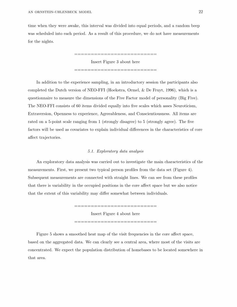
of the grid on Figure 3), when a pre-programmed wristwatch beeped (9 times a day).

Not surprisingly, some of the planned measurements were missing. If the participants

missed a beep, they had to indicate why they missed it, and in almost all cases the reason was

that they did not hear it. Therefore, the missing data were considered to be missing

completely at random (MCAR; Little & Rubin, 2002) and it was assumed that there was no

observation at that particular time (which makes the data unbalanced).

The average age of the participants was 21.7 years (SD = 4.7) and 60% of them were

women. The maximum number of measurements for a single person was 63 and on average

there were 60 measurements per person (SD = 3.4). The elapsed time interval between the

measurements was semi-random. The participants were asked to give information about the


time when they were awake, this interval was divided into equal periods, and a random beep

was scheduled into each period. As a result of this procedure, we do not have measurements

for the nights.

=========================


=========================

In addition to the experience sampling, in an introductory session the participants also

completed the Dutch version of NEO-FFI (Hoekstra, Ormel, & De Fruyt, 1996), which is a

questionnaire to measure the dimensions of the Five Factor model of personality (Big Five).

The NEO-FFI consists of 60 items divided equally into five scales which asses Neuroticism,

Extraversion, Openness to experience, Agreeableness, and Conscientiousness. All items are

rated on a 5-point scale ranging from 1 (strongly disagree) to 5 (strongly agree). The five

factors will be used as covariates to explain individual differences in the characteristics of core

affect trajectories.

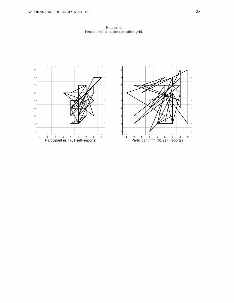
5.1. Exploratory data analysis

An exploratory data analysis was carried out to investigate the main characteristics of the

measurements. First, we present two typical person profiles from the data set (Figure 4).

Subsequent measurements are connected with straight lines. We can see from these profiles

that there is variability in the occupied positions in the core affect space but we also notice

that the extent of this variability may differ somewhat between individuals.

=========================


=========================

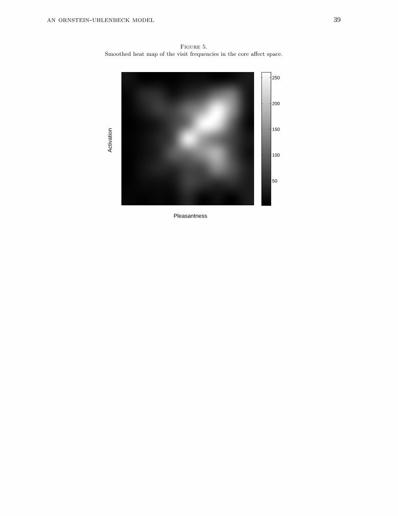
Figure 5 shows a smoothed heat map of the visit frequencies in the core affect space,

based on the aggregated data. We can clearly see a central area, where most of the visits are

concentrated. We expect the population distribution of homebases to be located somewhere in

that area.


=========================


=========================

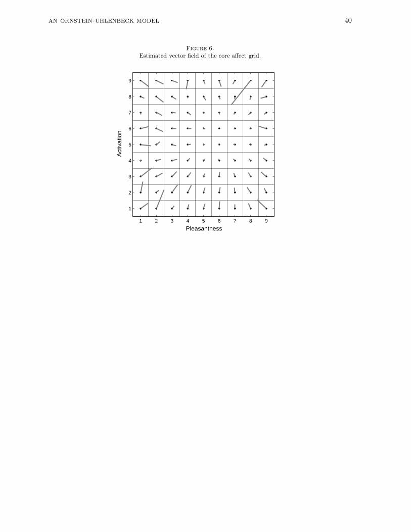
Figure 6 shows the estimated vector-field of the core affect grid with the data pooled

together for all individuals in the dataset. For each cell in the core affect grid, the length of

the vector is proportional to the estimated escape velocity from that cell and its angle

corresponds to the direction of escape. At the more central locations in the grid, the average

velocity to move away is very small. However, as farther away from this central point, there is

a tendency to be pulled towards the center: the directions of most of the vectors are more or

less toward the central location and with increasing distance from the central point, the vector

length tends to increase. (At the border cells, we notice more irregularity - these are due to

sampling variability because there are much fewer visits to these outer cells; see also the heat

map in Figure 5.)

=========================


=========================

5.2. Implementation of the MCMC algorithm

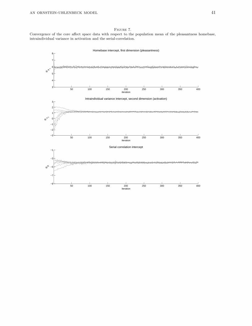
The results presented below are based on 36000 draws from the posterior distribution,

which come from six chains with 6000 iterations each. Each chain started with a burn-in

period, to be discarded, of length 4000. The initial values of the chains are randomly

perturbed rational values derived from the data (e.g., the sample average for the homebases).

Convergence checks showed no problems (all R < 1.1). Generally, the convergence was fast for

all parameters. Figure 7 shows the six iteration histories for three parameters (in each case

starting from different initial values).

=========================


=========================

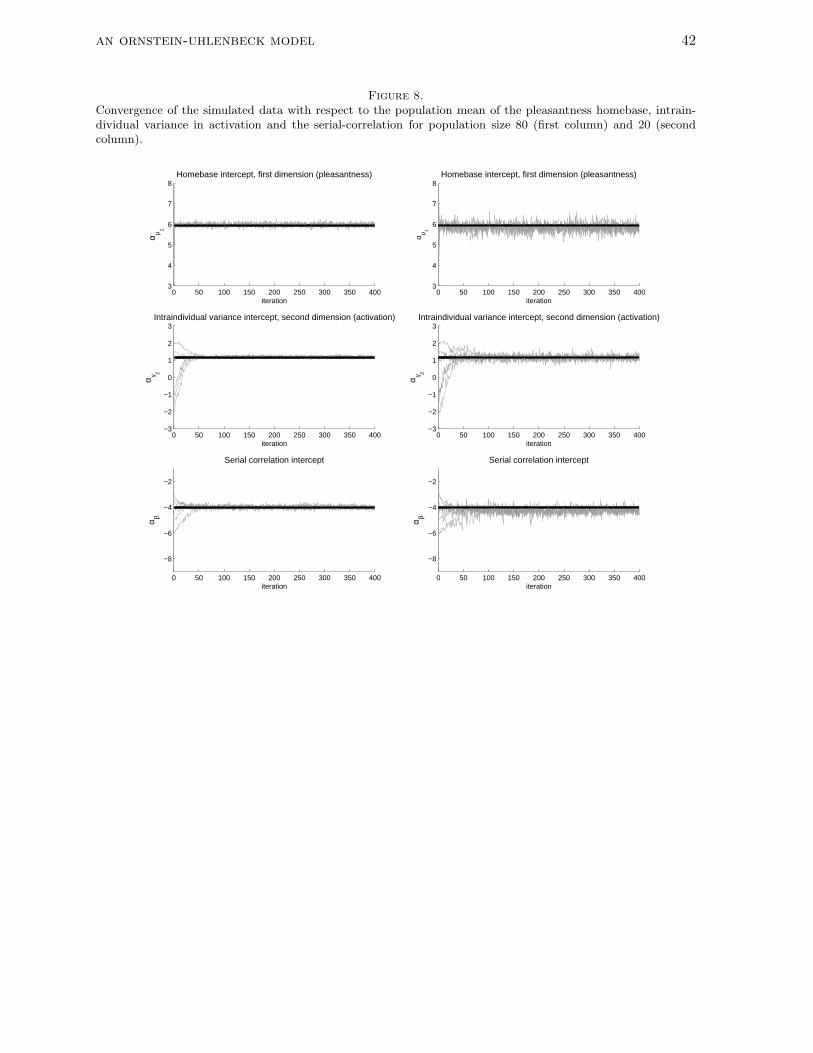
To demonstrate the efficiency, we ran some simulations for illustrative purposes. We

simulated two data sets with the estimated population means, but with different numbers of


people. Figure 8 shows the recovered population means with sample size 80, as in the

application in the first column and with sample size 20 in the second column. The black line

shows the simulated value. As can be seen, as the sample size increases, convergence is faster

and the uncertainty with respect to the mean decreases, but the model does reasonably well

with a relatively small sample size (20 subjects) as well.

=========================


=========================

5.3. Results

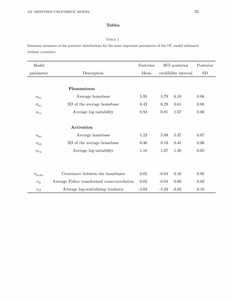
In a first step, we estimated the model without covariates to get a general description

about the core affect space (technically by reducing the covariate vector x′p to the scalar value

1 for each person). Table 1 shows a summary of the results, containing the posterior mean

(which is technically the intercept) and standard deviation and the endpoints of the 95%

posterior credibility interval. The estimated means of the homebase population distribution

are (5.95, 5.23), which correspond to the findings of previous research (Russell et al., 1989). It

shows that on average, the emotional state of persons is slightly pleasant and rather activated

than deactivated. If we look at the standard deviations of the homebases (0.42, 0.30) on the

two dimensions, it appears that there is an approximately equal amount of variability in the

homebases across persons. The covariance in the population between the homebases of the

dimensions is estimated to be 0.05, which means that across persons, the homebases of the

pleasantness and the activation dimensions are not related.

The average log-variance of the activation-deactivation dimension (1.18, which

corresponds to an expected mean of 3.65 on the normal scale) is somewhat larger than the

average log-variance of the pleasantness-unpleasantness dimension (0.94 i.e., 2.94 on the

normal scale). Considering the posterior mean of the Fisher transformed correlation in the

stationary distribution, it can be seen that the latter is rather small (i.e., 0.02), suggesting that

on average, there is not much cross-correlation (i.e., on average, the bivariate person-specific

stationary distributions have zero correlation). However, there is considerable variability in

the estimated person-specific untransformed cross-correlation parameters: The average value

is 0.02, while the between-person standard deviation is large (0.21), with the endpoints of the


95% credibility interval equal to −0.42 and 0.39, respectively. (It must be emphasized here

that there is a large conceptual difference between the population correlation of the homebase

distribution as discussed above – equal to 0.05 – and the average correlation of the stationary

distribution as discussed in this paragraph; both concepts are unrelated to each other.)

=========================

Insert Table 1 about here

=========================

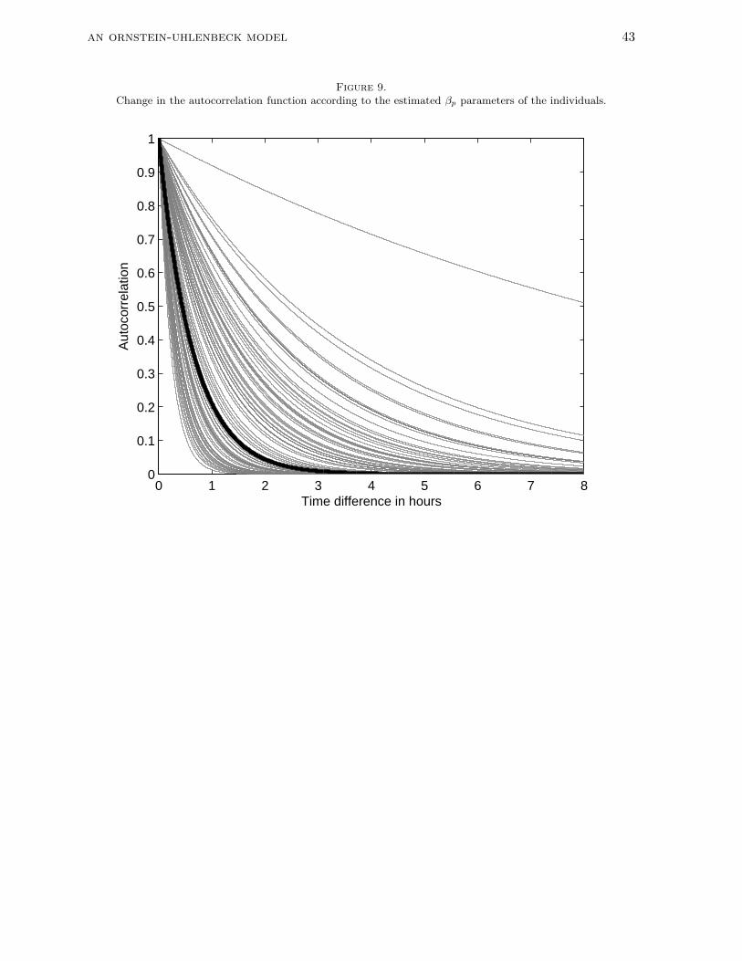
The mean of the population distribution of the logarithm of the centralizing tendency is

estimated to be −4.03. If we convert it back to the original scale, the estimate for the mean of

the population average centralizing tendency is 0.026. We may also look at the posterior

estimates for the person-specific centralizing force (i.e. βp). To illustrate the interpretation of

this average and the individual variation in centralizing tendency graphically, we convert the

posterior person-specific βp estimates to the corresponding autocorrelation functions. Figure 9

shows the person-specific autocorrelation function together with the autocorrelation functions

based on the average population value (thick line). For most participants, the autocorrelation

between subsequent core affect positions separated 2 hours in time is fallen below 0.2.

=========================


=========================

In a next step, each of the six person-specific Ornstein-Uhlenbeck parameters (i.e., the

two homebases µp and the log-variances log(γup) of the pleasantness-unpleasantness and the

activation-deactivation dimensions, the Fisher transformed cross-correlation between the

dimensions F (ρp) and the log-centralizing tendency log(βp)) were regressed onto the Big Five

personality dimensions. Table 2 summarizes posterior means and standard deviations for the

four regression coefficients for which the 95% posterior credibility intervals do not contain zero.

The current analysis shows that the neurotic individuals tend to have a lower homebase

with respect to pleasantness. Also, they show higher intra-individual variance in this

dimension. Based on these findings it seems that they generally feel quite unpleasant but it

changes dynamically, which might suggest emotional instability. In contrast, agreeable

individuals tend to have lower variation with respect to pleasantness.


The cross-correlation parameter presents another interesting aspect of the core affect

space. It shows how changes with respect to hedonic and arousal values coincide.

Interestingly, for conscientious individuals, changes in one dimension are negatively correlated

with the changes in the other one. In their case, high levels of pleasantness might often be

accompanied with relatively low levels of activation and vice versa.

The presented results are based on the basic OU model in which every diffusion parameter

was modeled as a random effect, that is, we assumed that people would differ from each other

with respect to all of the modeled variables. However, we can construct simpler models, by

removing individual difference dimensions from the model (i.e., restricting parameters to be

equal across persons) or by dropping parameters altogether. Three constrained models were

fitted and compared to the basic model using the DIC (estimated on 4000 posterior draws).

The DIC value of the basic model is 18103. In the first constrained model, we did not allow βp

to vary across persons, but we still estimated a non-person-specific β. The DIC of this model

is higher, namely 18366. Then we tested whether there is any need for autocorrelation in the

model at all by fixing β to a large value. The resulting DIC of this constrained model was

even higher, 19377, indicating that we indeed need to take into account the autocorrelation in

the model. Finally, we estimated a very simple constrained model where just the homebases

were person-specific. This model showed the highest DIC value (i.e., 19723). These outcomes

tend to confirm our assumption that people do differ with respect to the modeled parameters.

=========================

Insert Table 2 about here

=========================

6. Conclusion

In this paper, we have introduced a model for the analysis of multivariate longitudinal

profiles with continuous and possibly unbalanced measurement times. The presented

hierarchical diffusion modeling approach offers three distinctive characteristics.

First of all, in our approach a multivariate Ornstein-Uhlenbeck diffusion process serves as

a model for individual behavior. The OU diffusion process is an intuitively appealing way of

describing the continuous change of certain phenomena over time, certainly for constructs

related to mood and emotion. Although we must mention, that the current methodology is


developed for quantitative variables, and not yet able to deal with categorical or mixed

responses.

Second, we have succeeded in allowing for individual differences in all parameters of the

model. Traditionally, one only looks for between-person differences in the mean structure.

However, our application suggests that with respect to variation in core affect trajectories,

there are also differences between people in their variabilities, cross-correlations between the

dimensions and autocorrelations. The latter aspects are usually thought of as fixed over

persons. That there is individual variation in these features has been confirmed by regressing

the individual differences parameters on covariates and thereby explaining the existing

variation. Although we have only a single application, it holds interesting suggestions for

further substantive research in the core affect domain.

Third, we have fitted the model using a Bayesian approach. The parameter estimation

procedure is exact (in the sense that it is not an approximated model that is fitted) and

relatively fast (a single analysis takes only a few hours). Bayesian parameter estimation has

the advantage that relatively complex models (as the one described in this paper) can be

handled and that the uncertainty in the parameter estimates is easy to express (by means of

credibility intervals or even visually by plotting marginal posterior distributions). It also

provides a useful framework for model selection.

A major remaining challenge regarding the present modeling framework is the issue of

systematic model testing. In this paper, we have concentrated on model selection (i.e.,

selecting the best fitting model among a predefined set of possible models) using the DIC.

This is a common way of working in the domain on hierarchical or multilevel models where

model selection is carried out using approximative methods such as DIC, AIC or BIC (the

latter two employed in a non-Bayesian context). In addition, absolute measures of model fit

can also be considered but this is a far more involved issue not in the last place because of the

hierarchical nature of the model. Candidate procedures that could be considered involve, for

instance, the posterior predictive check framework (e.g., Gelman et al., 2004; Gelman,

Goegebeur, Tuerlinckx, & Van Mechelen, 2000).


References

Arnold, L. (1974). Stochastic differential equations: Theory and applications. New York: John

Wiley & Sons, inc.

Barnard, J., McCulloch, R. E., & Meng, X. L. (2000). Modeling covariance matrices in terms

of standard deviations and correlations, with application to shrinkage. Statistica Sinica,

10, 1281–1311.

Blackwell, P. G. (1997). Random diffusion models for animal movements. Ecological

Modelling, 100, 87–102.

Blackwell, P. G. (2003). Bayesian inference for Markov processes with diffusion and discrete

components. Biometrika, 90, 613–627.

Bolger, N., Davis, A., & Rafaeli, E. (2003). Diary methods: Capturing life as it is lived.

Annual Review of Psychology, 54, 579–616.

Bollen, K. A. (1989). Structural equations with latent variables. New Jersey, NJ: Wiley.

Borkenau, P., & Ostendorf, F. (1998). The big five as states: How useful is the five-factor

model to describe intraindividual variations over time? Journal of Research in

Personality, 32, 202–221.

Brillinger, D. R., Preisler, H. K., Ager, A. A., & Kie, J. G. (2004). An exploratory data

analysis (EDA) of the paths of moving animals. Journal of Statistical Planning and

Inference, 122, 43–63.

Brockwell, P. J., & Davis, R. A. (2002). Introduction to time series and forecasting. New

York: Springer-Verlag.

Cox, D. R., & Miller, H. D. (1972). The theory of stochastic processes. London: Chapman and

Hall.

Cruz-Mesıa, R. De la, & Marshall, G. (2006). Non-linear random effects models with

continuous time autoregressive errors: a Bayesian approach. Statistics in Medicine, 25,

1471–1784.

Csikszentmihalyi, M., & Larson, R. (1987). Validity and reliability of the experience sampling

method. The Journal of Nervous and Mental Disease, 175, 526–536.

Daniels, M., & Pourahmadi, M. (2002). Bayesian analysis of covariance matrices and dynamic

models for longitudinal data. Biometrika, 89, 553–566.

De Boeck, P., & Wilson, M. (2004). Explanatory item response models: A generalized linear


and nonlinear approach. New York: Springer.

Delsing, M. J. M. H., Oud, J. H. L., & Bruyn, E. E. J. (2005). Assessment of bidirectional

influences between family relationships and adolescent problem behavior: Discrete vs.

continuous time analysis. European Journal of Psychological Assessment, 21, 226–231.

Diggle, P. J., Heagerty, P., Liang, K. Y., & Zeger, S. L. (2002). Analysis of longitudinal data

(second edition). Oxford: Oxford University Press.

Dunn, J. E., & Gipson, P. S. (1977). Analysis of radio telemetry data in studies of home

range. Biometrics, 33, 85–101.

Ferrer, E., & Nesselroade, J. R. (2003). Modeling affective processes in dyadic relations via

dynamic factor analysis. Emotion, 3, 344–360.

Gelman, A., Carlin, J., Stern, H., & Rubin, D. (2004). Bayesian data analysis. New York:

Chapman & Hall.

Gelman, A., Goegebeur, Y., Tuerlinckx, F., & Van Mechelen, I. (2000). Diagnostic checks for

discrete-data regression models using posterior predicitive simulations. Journal of the

Royal Statistical Society Series C - Applied Statistics, 49, 247–268.

Goldstein, H. (2003). Multilevel statistical models. London: Arnold.

Hoekstra, H. A., Ormel, J., & De Fruyt, F. (1996). NEO PI-R, NEO FFI Big five

persoonlijkheidsvragenlijsten : Handleiding [NEO PI-R, NEO FFI Big five personality

questionnaire: Manual]. Lisse, The Netherlands: Swets & Zeitlinger B.V.

Karlin, S., & Taylor, H. (1981). A second course in stochastic processes. New York: Academic

Press.

Kuppens, P., Van Mechelen, I., Nezlek, J. B., Dossche, D., & Timmermans, T. (2007).

Individual differences in core affect variability and their relationship to personality and

adjustment. Emotion, 7, 262–274.

Larsen, R. J. (2000). Toward a science of mood regulation. Psychological Inquiry, 11, 129–141.

Larson, R., & Csikszentmihalyi, M. (1983). The experience sampling method. New Directions

for Methodology of Social and Behavioral Science, 15, 41–56.

Li, S. C., Huxhold, O., & Schmiedek, F. (2004). Aging and attenuated processing robustness:

Evidence from cognitive and sensorimotor functioning. Gerontology, 50, 28–34.

Little, R. J., & Rubin, D. B. (2002). Statistical analysis with missing data. New York: John

Wiley.


Lykken, D. T., & Tellegen, A. (1996). Happiness is a stochastic phenomenon. Psychological

Science, 7, 186–189.

Montfort, K. van, Oud, J., & Satorra, A. (2007). Longitudinal models in the behavioral and

related sciences. Mahwah, NJ: Lawrence Erlbaum Associates.

Mood, A. M., Graybill, F. A., & Boes, D. C. (1974). Introduction to the theory of statistics.

New York: McGraw-Hill.

Oud, J. H. L. (2002). Continuous time modeling of the crossed-lagged panel design.

Kwantitatieve Methoden, 69, 1–26.

Oud, J. H. L. (2007). Comparison of four procedures to estimate the damped linear

differential oscillator for panel data. In K. van Montfort, J. Oud, & A. Satorra (Eds.),

Longitudinal models in the behavioral and related sciences (pp. 19–40). Mahwah, NJ:

Lawrence Erlbaum Associates.

Oud, J. H. L., & Singer, H. (2008). Continuous time modeling of panel data: Sem versus filter

techniques. Statistica Neerlandica, 62, 4–28.

Raudenbush, S. W., & Bryk, A. S. (2002). Hierarchical linear models: Applications and data

analysis methods. Newbury Park, CA: Sage.

Robert, C. P., & Casella, G. (2004). Monte Carlo statistical methods. New York: Springer.

Russell, J. A. (2003). Core affect and the psychological construction of emotion. Psychological

Review, 110, 145–172.

Russell, J. A., & Feldman-Barrett, L. (1999). Core affect, prototypical emotional episodes,

and other things called emotion: Dissecting the elephant. Journal of Personality and

Social Psychology, 76, 805–819.

Russell, J. A., Weiss, A., & Mendelssohn, G. A. (1989). Affect grid: A single-item scale of

pleasure and arousal. Journal of Personality and Social Psychology, 57, 493–502.

Schach, S. (1971). Weak convergence results for a class of multivariate Markov processes. The

Annals of Mathematical Statistics, 42, 451–465.

Singer, H. (2008). Nonlinear continuous time modeling approaches in panel research.

Statistica Neerlandica, 62, 29–57.

Smith, P. L. (2000). Stochastic, dynamic models of response times and accuracy: A

foundational primer. Journal of Mathematical Psychology, 44, 408–463.

Spiegelhalter, D. J., Best, N. G., Carlin, B. P., & Linde, A. van der. (2002). Bayesian


measures of model complexity and fit (with discussion). Journal of the Royal Statistical

Society, Series B, 6, 583–640.

Sy, J. P., Taylor, J. M. G., & Cumberland, W. G. (1997). A stochastic model for the analysis

of bivariate longitudinal AIDS data. Biometrics, 53, 542–555.

Taylor, J. M. G., Cumberland, W. G., & Sy, J. P. (1994). A stochastic model for analysis of

longitudinal AIDS data. Journal of the American Statistical Association, 89, 727–736.

Verbeke, G., & Molenberghs, G. (2000). Linear mixed models for longitudinal data. New York:

Springer-Verlag.

Walls, T. A., & Schafer, J. L. (2006). Models for intensive longitudinal data. New York:

Oxford University Press.

Zellner, A. (1971). An introduction to Bayesian inference in econometrics. New York: Wiley.


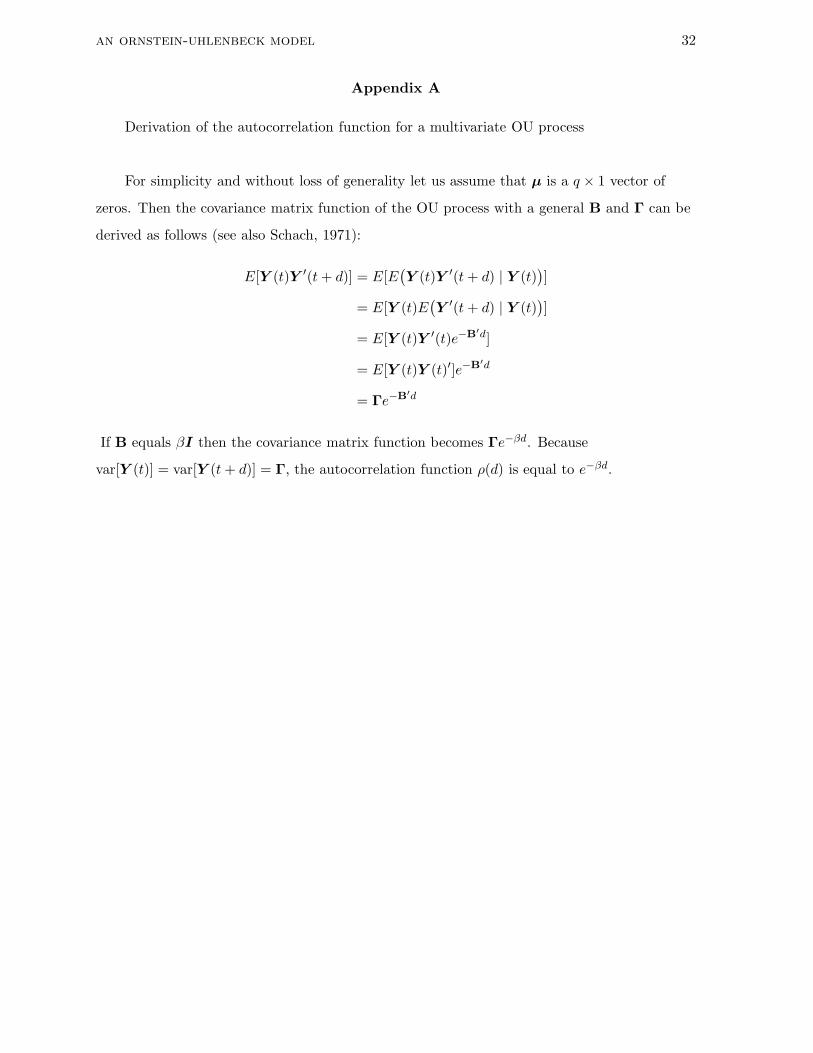
Appendix A

Derivation of the autocorrelation function for a multivariate OU process

For simplicity and without loss of generality let us assume that µ is a q × 1 vector of

zeros. Then the covariance matrix function of the OU process with a general B and Γ can be

derived as follows (see also Schach, 1971):

E[Y (t)Y ′(t + d)] = E[E(

Y (t)Y ′(t + d) | Y (t))

]

= E[Y (t)E(

Y ′(t + d) | Y (t))

]

= E[Y (t)Y ′(t)e−B′d]

= E[Y (t)Y (t)′]e−B′d

= Γe−B′d

If B equals βI then the covariance matrix function becomes Γe−βd. Because

var[Y (t)] = var[Y (t + d)] = Γ, the autocorrelation function ρ(d) is equal to e−βd.


Tables

Table 1.

Summary measures of the posterior distributions for the most important parameters of the OU model estimated

without covariates

Model Posterior 95% posterior Posterior

parameter Description Mean credibility interval SD

Pleasantness

αµ1 Average homebase 5.95 5.79 6.10 0.08

σµ1 SD of the average homebase 0.42 0.29 0.61 0.08

αγ1 Average log-variability 0.94 0.81 1.07 0.06

Activation

αµ2 Average homebase 5.23 5.09 5.37 0.07

σµ2 SD of the average homebase 0.30 0.19 0.45 0.06

αγ2 Average log-variability 1.18 1.07 1.30 0.05

σµ1µ2 Covariance between the homebases 0.05 -0.04 0.16 0.05

αρ Average Fisher transformed cross-correlation 0.02 -0.04 0.08 0.03

αβ Average log-centralizing tendency -4.03 -4.23 -3.82 0.10


Table 2.

Summary of the regression coefficients with a 95% posterior credibility not containing 0.

Model Posterior 95% Posterior Posterior

parameter Description Covariate mean credibility interval SD

Pleasantness

αµ1N Homebase Neuroticism -0.38 -0.64 -0.11 0.13

αγ1N Variability Neuroticism 0.23 0.01 0.45 0.11

αγ1A Variability Agreeableness -0.29 -0.58 -0.00 0.14

αρC Cross-correlation Conscientiousness -0.17 -0.29 -0.06 0.06

Note. Model parameters refer to the regression weights. For example αµ1N is the regression

weight for neuroticism relating to the homebase in the pleasantness dimension (µ1).


Figures

Figure 1.

The 0.5 probability contour curves of conditional distributions - the centers denoted by ×-s - with three differentvalues for β.

0 1 2 3 4 5 6 7 8 90

1

2

3

4

5

6

7

8

9

Homebase Previous point

Small β

Medium β

Large β

Y(1)

Y(2)


Figure 2.

Four different β values and their corresponding autocorrelation functions.

0 50 100 150 200 250 300 350 4000

0.1

0.2

0.3

0.4

0.5

0.6

0.7

0.8

0.9

1

time difference

auto

corr

elat

ion

β=0.01

β=0.02

β=0.03

β=0.04


Figure 3.

The Affect Grid used in the application.


Figure 4.

Person profiles in the core affect grid.

1 2 3 4 5 6 7 8 9

1

2

3

4

5

6

7

8

9

Participant nr.7 (61 self−reports)1 2 3 4 5 6 7 8 9

1

2

3

4

5

6

7

8

9

Participant nr.4 (61 self−reports)


Figure 5.

Smoothed heat map of the visit frequencies in the core affect space.

Pleasantness

Act

ivat

ion

50

100

150

200

250


Figure 6.

Estimated vector field of the core affect grid.

1 2 3 4 5 6 7 8 9

1

2

3

4

5

6

7

8

9

Pleasantness

Act

ivat

ion


Figure 7.

Convergence of the core affect space data with respect to the population mean of the pleasantness homebase,intraindividual variance in activation and the serial-correlation.

50 100 150 200 250 300 350 4003

4

5

6

7

8Homebase intercept, first dimension (pleasantness)

iteration

α µ 1

50 100 150 200 250 300 350 400−3

−2

−1

0

1

2

3Intraindividual variance intercept, second dimension (activation)

iteration

α γ 2

50 100 150 200 250 300 350 400

−1

−3

−5

−7

−9

Serial correlation intercept

iteration

α β


Figure 8.

Convergence of the simulated data with respect to the population mean of the pleasantness homebase, intrain-dividual variance in activation and the serial-correlation for population size 80 (first column) and 20 (secondcolumn).

0 50 100 150 200 250 300 350 4003

4

5

6

7


iteration

α µ 1

0 50 100 150 200 250 300 350 400−3

−2

−1

0

1

2


iteration

α γ 2

0 50 100 150 200 250 300 350 400

−8

−6

−4

−2


iteration

α β

0 50 100 150 200 250 300 350 4003

4

5

6

7


iteration

α µ 1

0 50 100 150 200 250 300 350 400−3

−2

−1

0

1

2


iteration

α γ 2

0 50 100 150 200 250 300 350 400

−8

−6

−4

−2


iteration

α β


Figure 9.

Change in the autocorrelation function according to the estimated βp parameters of the individuals.

0 1 2 3 4 5 6 7 80

0.1

0.2

0.3

0.4

0.5

0.6

0.7

0.8

0.9

1

Time difference in hours

Aut

ocor

rela

tion

A Hierarchical Ornstein–Uhlenbeck Model for Continuous Repeated Measurement Data

Documents

Transcript of A Hierarchical Ornstein–Uhlenbeck Model for Continuous Repeated Measurement Data