A hierarchical latent class model for predicting disability

small area counts from survey data

Enrico Fabrizi∗ Giorgio E. Montanari† M. Giovanna Ranalli‡

April 19, 2012

Abstract

This article considers the estimation of the number of severely disabled people using

data from the Italian survey on Health Conditions and Appeal to Medicare. Disability

is indirectly measured using a set of categorical items, which survey a set of functions

concerning the ability of a person to accomplish everyday tasks. Latent Class Models

can be employed to classify the population according to different levels of a latent

variable connected with disability. The survey, however, is designed to provide reliable

estimates at the level of Administrative Regions (NUTS2 level), while local authorities

are interested in quantifying the amount of population that belongs to each latent class

at a sub-regional level. Therefore, small area estimation techniques should be used.

The challenge of the present application is that the variable of interest is not observed.

Adopting a full Bayesian approach, we base small area estimation on a Latent Class

model in which the probability of belonging to each latent class changes with covariates

and the influence of age is learnt from the data using penalized splines. Deimmler-

Reisch bases are shown to improve speed and mixing of MCMC chains used to simulate

posteriors.

Keywords: Small area estimation; Unit level model; Penalized splines; Demmler-Reinsch

bases; Nonparametric regression; Health interview survey.

1 Introduction

Aging of the population, in particular when it is connected with a status of disability, is

a central issue for policy makers in most OECD countries. Severe disability may cause

a condition of autonomy deprivation so that the individual needs personal assistance to

complete basic everyday tasks. Decision makers, responsible for health organization and

∗DISES, Universita Cattolica del S. Cuore, Piacenza, Italy†DEFS, Universita degli Studi di Perugia, Italy‡DEFS, Universita degli Studi di Perugia, Italy, giovanna.ranalli@stat.unipg.it

1

arX

iv:1

204.

3993

v1 [

stat

.AP]

18

Apr

201

2

planning are very interested in classifying the population and monitoring the number of

people with different levels of disability in order to determine the care needs in a territory

and configure appropriate social policies.

Assessment of levels of functioning and disability can be conducted on a personal basis

via interviews and medical investigation by a medical staff from Local Health Depart-

ments on each person who requests benefits and extra sanitary assistance. However, such

information does not provide sufficient data for classifying the population according to the

different levels of disability, since it does not include all those people who do not formally

inquire for extra public sanitary assistance and, also, different scales are used in the clas-

sification by each Department. It is therefore very important to be able to estimate the

impact of the phenomenon using an alternative data source. Since ah hoc surveys are too

expensive, we propose to use data from some existing extensive surveys on the population

routinely run by National Statistical Institutes.

In this work we look in particular at the case of Italy – that shows the largest propor-

tion of population aged 65 or more among EU25 European countries, 20.3% in 2011. The

most structured and complete data source on disability in Italy is the Health Conditions

and Appeal to Medicare Survey (HCAMS) conducted by the National Institute of Statis-

tics every five years. The most recent available edition is that from the years 2004-05.

The HCMAS employs a questionnaire that accounts for the International Classification of

Impairments, Disabilities and Handicaps (ICIDH) developed by the World Health Orga-

nization in 1980 and evaluates disability by means of 14 items that include the Activities

of Daily Living (ADL; Katz et al., 1963). In this survey a person is considered as disabled

if, excluding temporary limitations, he/she expresses the largest degree of difficulty in at

least one of a set of functions concerning the ability of a person to accomplish everyday

tasks such as getting washed and dressed, eating, walking or hearing, even with the aid of

tools such as glasses, walking sticks, prostheses. More details on the items are provided in

Section 2. From a policy maker perspective, this definition of disability is way too loose,

in that a person may be defined as disabled because he/she cannot hear a TV-show, but

he/she can perfectly take care of him/herself without an extra-burden for the Health Care

system. In fact, what is mainly interesting for policy making and planning is to evaluate

that level of disability that is connected with a status of dependency.

ADLs have been used extensively to detect disability. The basic approach to measuring

disability is by using a summed index, where individual scores on all items are summed

to produce a total. One obvious sufficient condition for the summed index (total score)

to be valid is that all items equally contribute to some sort of measure of disability, a

condition that may not hold. Tools from Item Response Theory may be applied to obtain

a proper aggregate measure of functional disability. Erosheva (2002) provides a review of

application of such models to ADLs. See also Cabrero-Garcıa and Lopez-Pina (2008) for

2

the use of ADLs to obtain an aggregate measure of functional disability from a national

survey in Spain. To classify the population according to different levels of disability, Latent

Class Models (Lazarsfeld and Henry, 1968) can be employed. Montanari et al. (2011) use

this approach on data from the HCAMS to classify people and are able to identify, among

the others, one class as composed by those in a condition of severe disability. In this work

we follow this approach, but we extend it to tackle the following issues.

The survey uses a stratified two stage sampling design and provides direct estimates

reliable up to the Administrative Region level (NUTS2). In this work we focus, within

Italy, on the case of the Administrative Region Umbria. It is located in the center of Italy

and shows the second largest proportion of people aged 65 or more in the nation (23.1%).

Like all Regions in Italy, Umbria is divided into 12 Health Districts and the local Ad-

ministrative Department responsible for health organization and planning is interested in

classifying the population according to different levels of disability for each Health Dis-

trict and age class (50-64; 65-74; 75 and more). Once a unit in the sample is labelled with

his/her most probable latent class, reliable direct estimates of the amount of population

within each District and age class cannot be obtained due to the lack of a sufficient number

of observations. Small area estimation techniques should then be used to obtain estimates

for the 12 Health Districts by the 3 age classes. The basic idea of small area estimation

is to introduce a model to exploit the relationship between the variable of interest and

some auxiliary variables for which information at the population level is available (such

information may range from population counts at the small area level to individual popu-

lation records). A great deal of research has been devoted to this field of survey statistics

in recent years (for reviews see Rao, 2003; Jiang and Lahiri, 2006). However, the challenge

of the present application is that the variable of interest is not observed; it is a latent

variable hidden in the items surveyed. Small area estimation techniques have not been

developed for estimating the total or the mean of a latent variable.

A first solution may be a two step procedure in which (1) item responses of every unit

are summarized to obtain a measurement of the latent variable; this is done by fitting a

latent class model to the data and label each unit with his/her most probable class. Then

(2) measurements (latent class memberships) are used as a known dependent variable in

a small area model (e.g. a multinomial mixed effects model as in Ghosh et al., 1998).

This solution is unsatisfactory, since when using latent variable estimates in a regression

model, the association between the real value of the latent variable and the covariates is

underestimated (Mesbah, 2004). In addition, errors are propagated from step (1) to step

(2) without any control. We propose to tackle the problem of classifying the population

and getting small area estimates as a whole within a Hierarchical Bayesian framework

in which the probability of belonging to each latent class changes with covariates. Age

by sex by marital status counts are available for each municipality from administrative

3

registers and can be used as covariates. A random effect capturing the variability between

the districts not accounted for by the covariates is also introduced.

No parametric assumption on the functional form of the influence of age is made. We

therefore extend the latent class mixed effects model with covariates to the case in which

the effect of a continuous variable is only assumed to be a smooth function. Penalized spline

(p-spline) regression is then used to approximate this function (see Eilers and Marx, 1996;

Ruppert et al., 2003, for a general treatment of p-splines and their applications). Opsomer

et al. (2008) exploit the mixed models representation of p-splines (see Ruppert et al., 2003,

Chapt. 4) to incorporate it in a small area model. The smooth function can be modeled

using natural cubic splines, B-splines, truncated polynomials, radial splines and others. In

Bayesian analysis based on MCMC methods, the particular choice of basis is crucial for

its consequences on the mixing of the MCMC chains. Crainiceanu et al. (2005) provide

an overview of the implementation of nonparametric Bayesian analysis via p-splines and

advocate the use of low-rank thin-plate splines for their good mixing properties of the

MCMC chains. Since we are modeling a latent variable, even the use of this basis yields

a large posterior correlation for the fixed and the random coefficients in the mixed model

representation of the p-spline. In this work we propose the use of the Demmler-Reinsch

basis (Nychka and Cummins, 1996). Like B-splines, they provide a transformation of basis

that implies an orthogonal design matrix. The latter property allows for a much better-

behaved chains and a reduction of computational time.

The paper is organized as follows. Section 2 provides an overview of the survey data

and the items employed to measure disability. Section 3 illustrates the alternative mod-

els employed, describes the model and the p-splines specification. Section 4 shows the

final results after the procedure of model selection and checking. Section 5 provides some

concluding remarks and directions for future research.

2 The data

The target population for the HCAMS is that of households. The survey design uses a

complex sampling scheme and, in particular, it is as follows. Within a given Province

(LAU1), municipalities are classified as Self-Representing Areas (SRAs) - consisting of

the larger municipalities - and Non Self-Representing Areas (NSRAs) - consisting of the

smaller ones. In SRAs each municipality is a single stratum and households are selected

by means of systematic sampling. In NSRAs the sample is based on a stratified two stage

sample design. Municipalities are primary sampling units (PSUs), while households are

Secondary Sampling Units (SSUs). PSUs are divided into strata of approximately the same

dimension in terms of population. One PSU is drawn from each stratum with probability

proportional to the PSU population size. The SSUs are selected by means of systematic

4

Table 1: Number of observations available for each domain of interest given by Health

district by age class. Health districts are ordered by code.

50− 64 65− 79 ≥ 80

[11] Alto Tevere 32 41 10

[12] Alto Chiascio 52 40 18

[21] Perugino 117 81 26

[22] Assisano 27 24 8

[23] Medio Tevere 28 27 13

[24] Trasimeno 26 22 7

[31] Valnerina 14 13 5

[32] Spoleto 41 45 22

[33] Foligno 88 82 31

[41] Terni 120 78 30

[42] Narni 36 35 11

[43] Orvieto 39 40 11

sampling in each PSU. All members of each sample household, in both SRAs and NSRAs,

are interviewed. The survey is designed to provide reliable estimates at a regional level

(NUTS2). Note that all those who live permanently in a care facility are not included in

the sample.

The 2004-05 edition of the HCAMS has involved in Umbria 1,210 households and 3,088

people divided into 40 municipalities. Since in this work we are interested in people aged

50 or more, the available sample size reduces to 1,340. In addition, Umbria is divided into

12 Health districts, that are groups of neighboring municipalities. Table 1 provides the

sample size for each subpopulation given by the intersection of each health district with

each of 3 age classes. Many domains have very few observations (less than 30) available,

making it very unreliable to use direct estimation techniques.

To measure disability, the HCAMS accounts for the International Classification of

Impairments, Disabilities and Handicaps (ICIDH) developed by the World Health Orga-

nization in 1980. It provides a conceptual framework for disability, which is described in

three dimensions: impairment, disability and handicap. In the context of health experi-

ence an impairment is any loss or abnormality of psychological, physiological or anatomical

structure or function. On the other side, a disability is any restriction or lack (resulting

from an impairment) of ability to perform an activity in the manner or within the range

considered normal for a human being, whilst a handicap is a disadvantage for a given indi-

vidual, resulting from an impairment or a disability, that limits or prevents the fulfillment

of a role that is normal (depending on age, sex, and social and cultural factors) for that

5

individual. As we said before, in the HCAMS, a person is considered disabled if, excluding

temporary limitations, he/she expresses the largest degree of difficulty in at least one of

a set of functions concerning the ability of a person to accomplish everyday tasks, even

with the aid of tools.

Such functions are evaluated by means of 14 items in the questionnaire that include

the Activities of Daily Living (ADL; Katz et al., 1963). Four types of disability are de-

fined according to the kind of deprived functional autonomy: confinement, difficulties in

movement, difficulties in everyday activities and tasks, sensory deprivation. A condition

of permanent constriction in bed, on a chair or at one’s home due to physical or psychical

reasons is intended for confinement. People with difficulties in movements show problems

in walking, i.e. they can only walk few steps before taking a rest, they cannot climb the

stairs without stopping, they cannot bend to pick up something from the ground. Difficul-

ties in the activities of daily living are concerned essentially with a lack of independence

in accomplishing basic everyday tasks as going to bed, sitting, getting dressed or washed,

taking a bath or a shower. Finally, sensory deprivation includes limitations in hearing –

e.g. not being able to listen to a TV show even at a high volume, in spite of the use of

hearing aid; limitations in seeing – e.g. not being able to recognize a friend at a meter

distance; limitations in talking. The items are all ordinal with categories increasing with

the difficulty of fulfilling the task and they are grouped according to the aforementioned

four types of disability. The items (and corresponding categorization) follow.

1. Confinement:

– CONF = type of confinement (four categories: not confined, confined to one’s

home, confined to a chair, confined to one’s bed).

2. Difficulties in movements

– DIST = longest walkable distance (three categories: more than 200 m., less

than 200 m., only a few steps);

– STAIR = going up and down the stairs (four categories: capable, with some

effort, only with a lot of effort, not capable);

– STOOP = stooping down (four categories as for STAIR).

3. Difficulties in everyday activities and tasks

– BED = getting in and out of bed (three categories: with no effort, with some

effort, only with the help of somebody);

– CHAIR = sitting and standing (three categories as for BED);

– DRESS = getting dressed and undressed (three categories as for BED);

– BATH = taking a bath or a shower (three categories as for BED);

– WASH = washing one’s face and hands (three categories as for BED);

6

– EAT = eating cutting one’s food (three categories as for BED);

– CHEW = chewing (four categories as for STAIR);

4. Sensory deprivation

– HEAR = hearing a TV show (three categories: capable, only at high volume,

not capable);

– SIGHT = seeing and recognizing a friend (three categories: capable, only at a

meter distance, not capable);

– SPEE = speaking (three categories as for BED).

Montanari et al. (2011) consider the same set of items to provide a classification of the

elderly. In addition, they use the tools developed for the validation of Rasch models and

perform item fit analysis to assess which items provide a unidimensional latent construct.

Item fit analysis has been conducted on the dataset at hand here and results are in line with

those found in Montanari et al. (2011). In particular, out of the aforementioned 14 items,

nine are selected that provide a valid and reliable scale. In particular, CONF, CHEW,

HEAR, SEE and SPEE are removed from the analysis. This is in line with the literature

that raises concerns when merging “motor” and “cognitive” items. In addition, note that

CONF is indeed a so called “summary item” and is found to be redundant with respect to

motor items, while sensory deprivation items are found to have a very little discrimination

power when used in a latent class model. For all these reasons, in the following sections

we employ this reduced set of nine items to fit the latent class small area model.

3 The latent class small area model

In this section the proposed methodology to tackle the aforementioned problem is pre-

sented in detail. First, the structure of the model is provided: a latent class model is

coupled with a small area unit level model in which the probability of belonging to each

latent class is modeled via a multinomial mixed effects model. Sex, marital status and

age are considered as covariates. Note that the choice for covariates in a small area model

is limited to those for which population level information is available. In the present ap-

plication, in fact, better predictors of disability could be the presence of morbidities or

chronic diseases. Such information, although present in the HCAMS, is not supported by

the knowledge of population counts in municipalities or health districts. The effect of age

does not have a pre-specified parametric form and is learnt from the data using penal-

ized splines. Section 3.2 provides details on this issue. Then, parameter estimates for the

model are obtained within a Hierarchical Bayesian framework. The prior specification of

the model is then provided, together with the form of the small area estimates.

7

3.1 Model specification

Let Yijt denote the response of unit i within small area j = 1, . . . , J on item t = 1, . . . , T .

The number of small areas obtained by cross-classifying districts and age classes is denoted

by J = 12× 3, the number of units in the sample for small area j is nj so that the overall

sample size is given by n =∑J

j=1 nj . The total number of items is T = 9, while a particular

level of item t is denoted by ht and its number of categories by Ht. The latent class variable

is denoted by Qij , a particular latent class by c and the number of latent classes by C.

The full vector of responses of unit i in small area j is denoted by Y ij , whilst h refers to

a possible answer pattern.

If Nj is the population size of small area j, we are interested in estimating the small

area totals

Qj(c) =

Nj∑i=1

I(Qij = c),

for j = 1, . . . , J and c = 1, . . . , C, where I(·) denotes the indicator function. The latent

class small area model can be expressed asP (Y ij = h) =

∑Cc=1 P (Qij = c)P (Y ij = h|Qij = c),

logP (Qij = c)

P (Qij = 1)= α0c + vd(i)c + α1csexij + fc(ageij)+

+γcmarital-statusij , for c = 2, . . . , C.

(1)

The first equation is the latent class model in which the probability of observing a response

pattern h is a weighted average of class-specific probabilities. In fact, the term P (Y ij =

h|Qij = c) is the conditional response probability of observing pattern h given that unit i

in small area j belongs to class c, and the weight is the probability that such unit belongs

to the latent class c. By assuming independence of responses within latent classes, the

conditional probability takes the form

P (Y ij = h|Qij = c) =

T∏t=1

P (Yijt = ht|Qij = c). (2)

The probabilities P (Qij = c) are modeled via the multinomial logistic mixed model

of the second equation in which the first latent class is the reference one. Sex (reference

category is ‘female’) and marital status (with three binary variables – ‘married’, ‘sepa-

rated/divorced’, ‘widow’ – reference category is ‘single’) enter this model parametrically,

while fc(·), for c = 2, . . . , C, is a smooth function of age to be estimated nonparametrically.

Details on this latter aspect of the model are provided in Section 3.2. Finally, vd(i)c is a

zero mean random variable, for d = 1, . . . , 12 and c = 2, . . . , C, and d(i) denotes the health

district which unit i belongs to. These terms represent random intercepts included for each

health district to capture the between-district variation not explained by the covariates.

8

It is common practice in small area estimation to include a random intercept to model the

intra-area correlation and the area effect not accounted for the covariates in the model.

Once prior distributions are assumed on model parameters, a Markov Chain Monte

Carlo algorithm can be used to obtain M samples from the joint posterior distribution.

Prior choice and MCMC specifications are described in Section 3.3.

Since the small area part of model (1) is a multinomial mixed effect model, C − 1

different sets of fixed coefficients for sex and marital-status, of random intercepts for

the district effect and of smooth curves for age are estimated, one for each latent class

but the reference one. The latent variable can be considered univariate for the item fit

analysis described in Section 2; therefore, a more parsimonious model can be considered

that assumes ordered classes and fits a common effect for the covariates and a different

intercept for each class. If we consider a proportional odds model (see e.g. Agresti, 2002,

Chapt. 7), the second equation of (1) becomes

logitP (Qij ≤ c) = logP (Qij ≤ c)P (Qij > c)

= α0c + vd(i) + α1sexij + f(ageij) + γmarital-statusij , (3)

for c = 1, . . . , C − 1. Note that in equation (3) a common effect from the covariates for

different c is considered, and this is reasonable when a continuous variable is assumed to

underlie the variable Q. On the other hand, a different intercept α0c is included for each

latent class. These values are increasing in c, since P (Qij ≤ c) increases in c for a fixed

value of the covariates, and the logit is an increasing function of this probability. Moreover,

they can be interpreted as ‘cutpoints’ for the continuous underlying variable, that is Q is

equal to c when the underlying variable takes value in the interval (α0c−1, α0c].

3.2 Penalized spline regression

The effect of age in both models (1) and (3) does not have a pre-specified functional form,

but is only assumed to be a smooth function. A nonparametric model has significant

advantages compared with a parametric approach when the functional form of the rela-

tionship between the variable of interest and one or more covariates cannot be specified

a priori, since erroneous specification of the model can result in biased estimates. This is

particularly relevant in the present application, where the variable of interest is latent and

no clear way exists of predetermining a reasonable specific functional form for the effect

of age.

Despite the numerous extensions to the basic small area models present in literature,

the inclusion of a nonparametrically specified term in a small area model has only re-

cently been considered, due to the methodological difficulties of incorporating smoothing

techniques into the estimation tools used to this end. Opsomer et al. (2008) exploit the

9

close connection between penalized splines (p-splines) and linear mixed models (see e.g.

Ruppert et al., 2003, Chapt. 4) to incorporate a nonparametric mean function specifica-

tion into a small area unit level model. The p-spline representation of the smooth function

fc(ageij) in (1) is given by

fc(ageij ;βc, b1c, . . . , bKc) = βcageij +K∑k=1

bkczijk, (4)

where βc, b1c, . . . , bKc are regression coefficients, zijk are basis functions used to model

the smooth function, e.g. natural cubic splines, B-splines, truncated polynomials, radial

splines and others, that depend on a set of fixed knots κ1 < κ2 < . . . < κK . The number

of knots K has to be large enough to ensure the desired flexibility (Ruppert et al., 2003,

Chapt. 5, suggest to use one knot every 4 or 5 unique values for the covariate, with a

maximum number of 35), and they should be chosen to be nicely scattered over the range

of the covariate, with quantiles being a good choice. As of the choice of the spline basis,

while it makes a little difference in a classical framework, it is particularly relevant in a

Bayesian approach, for its consequences on the mixing properties of the MCMC chains.

Crainiceanu et al. (2005) offer details for p-splines smoothing within a Bayesian framework

and advocate the use of thin-plate splines, for which they notice a posterior correlation of

parameters that is much smaller than for other basis. In this case zijk = |ageij − κk|3.To avoid overfitting, the magnitude of the coefficients of the basis bkc, for k = 1, . . . ,K,

is penalized by shrinking it towards zero. This can be accomplished by considering βc as

an independent parameter and bc = (b1c, . . . , bKc)T as a vector of random parameters with

E(bc) = 0 and E(bcbTc ) = σ2bcΩ

−1K , where the (l, k)-th entry of ΩK is given by |κl − κk|3.

In this paper we propose to use the Demmler-Reinsch orthogonalization of a set of basis

functions (any set, not necessarily thin-plate splines) to improve the mixing of the MCMC

chains and eliminate the posterior correlation of βc and of bc. To this end, the following

steps have to be implemented. In particular, given zijk, let zij = (1, ageij , zij1, . . . , zijK),

let Z be the n × (K + 2) matrix whose ij-th row is given by zij , let bc = (α0c, βc, bTc )T

and let

D =

[02×2 02×K

0K×2 ΩK

].

Then, let R be a square (K+2)×(K+2) upper triangular invertible matrix so that RTR is

the Cholesky decomposition of ZTZ. The singular value decomposition of the symmetric

matrix R−TDR

−1, where R

−Tis the transpose of R

−1, is given by Udiag(s)U

T. For ease

of notation let the entries of the vector s be arranged in an increasing fashion. Then, given

the nature of D, the first two entries of s are equal to zero, i.e. s = (0, 0, sT )T .

Now, if we compute A = ZR−1U , then the columns of A identify the set of basis

functions known as the Demmler-Reinsch basis and show the orthogonality property. In

10

addition, given the ordering of s, and then of the columns of U , the columns of A will

exhibit more oscillations from the first to the (K + 2)-th and, in particular, they will

intersect the x-axis ν − 1 times, for ν = 1, . . . ,K + 2 (see Nychka and Cummins, 1996, for

more details on these aspects of Demmler-Reinsch bases).

Then, the transformation is given by

Zbc = ZR−1UU

TRbc = Awc, (5)

where wc = (ω0c, ω1c,wTc )T . If we denote by A the matrix made of the last K columns of

A, then equation (4) can be rewritten as

fc(ageij ;βc, w1c, . . . , wKc) = βcageij +K∑k=1

wkcaijk, (6)

where aijk is the (ij, k)-th element of A. In (6), βc is considered like in (4) as a fixed

parameter, while wc as a vector of random parameters with E(wc) = 0 and E(wcwTc ) =

σ2bcdiag(s)−1. The latter form of the variance of wc is obtained as follows. From (5) wc =

UTR22bc, where UT and R22 are defined from

U =

[I2×2 02×K

0K×2 U

]and R =

[R11 R12

0K×2 R22

],

respectively. Then,

E(wcwTc ) = σ2bcU

TR22Ω−1K R

T22U = σ2bcU

T (Udiag(s)UT )−1U = σ2bcdiag(s)−1,

because

R−TDR

−1=

[02×2 02×K

0K×2 R−T22 ΩKR−122

],

and

Udiag(s)UT

=

[I2×2 02×K

0K×2 Udiag(s)UT

].

3.3 Prior specification

To complete the Bayesian specification of the model we need to choose priors for the

parameters involved in equation (1): the conditional probabilities P (Y ij = h|Qij = c),

the regression parameters (α0c, α1c, βc, γc), for c = 2, . . . , C and the two sets of random

effects vc, bc – or vc, wc – for c = 2, . . . , C. For the conditional probabilities in (2) we

assume

P (Yijt = ht|Qij = c) ∼ Dirichlet(1Ht)

for t = 1, . . . , T , where 1Ht is a vector of ones with a length given by Ht, i.e. by the number

of categories of item t. The choice of this prior is customary and implies independent

uniform priors on the probability of selecting each level of the item being considered.

11

For the regression parameters α0c, α1c, βc and γc we assume diffuse normal priors with

mean 0 and variance 100 that are sufficiently non-informative and computationally more

convenient than flat priors over the real line.

For the random effects multivariate normality is assumed. For the health district effects,

we also assume a priori independence:

vdcind∼ N(0, σ2vc),

for d = 1, . . . , 12 and c = 2, . . . , C. On the other hand, for the random effects used in the

p-spline representation, consistently with section 3.2 we have:

bc ∼ MVN(0, σ2bcΩ−1K ),

when thin-plate splines are used – equation (4) – and

wc ∼ MVN(0, σ2bcdiag(s)−1),

when the Demmler-Reinsch orthogonalization is employed – equation (6). The normality

of the random effects is a standard assumption in hierarchical models including those used

in representing splines (Crainiceanu et al., 2005); moreover departures from normality of

random effects are very hard to detect (Fabrizi and Trivisano, 2009).

To complete the prior specification, we need to set prior distributions for the variance

components σ2bc and σ2vc for c = 1, . . . , C. This task is critical as in Bayesian mixed models

the posterior distributions of these parameters are known to be sensitive to prior spec-

ification (Gelman, 2006). In particular, the choice of the prior for σ2bc is crucial as this

parameter influences the smoothness of the p-splines. We assume the following prior for

the random effects standard deviation:

σbc ∼ Uniform(0, B)

c = 1, . . . , C. The use of uniform priors for the square root of the variance components

is discussed in Gelman (2006). The same prior is adopted for the standard deviation

associated to the health district effects:

σvc ∼ Uniform(0, B).

The choice of the prior for the variance components along with a sensitivity analysis

exercise and a discussion of how the value of B has been selected is contained in Section

4.2. When the small area model is based on equation (3), the prior specification is the

same for the subset of regression coefficients and random components considered.

12

3.4 Small area estimates

The posterior distributions for the parameters of our model cannot be obtained in closed

form. We use MCMC software to generate samples from the posterior distributions. The

posterior distributions of the counts for the different disability classes in the age by district

domains are simulated combining draws from the posterior distributions of model parame-

ters and population counts accurately known from population registers. In particular, from

administrative registers, we know age × sex × marital-status × district popula-

tion counts N`, for ` = 1, . . . , L = 50× 2× 4× 12. Note that 50 is the number of different

ages of persons in the sample (they range from 51 to 100). Specifically, the posterior mean

of the counts for the class c in small area j is obtained as follows:

Qj(c) =1

M

M∑m=1

∑`∈`j

N`P(m)(Q` = c|vd(`)c, age`, sex`, marital-status`) (7)

where

• m indexes the MCMC runs and M is their number,

• ` is a particular cell and `j is the subset of cells from the total L that is contained

in the small area j,

• and the probabilities P (m)(Q` = c|vd(`)c, age`, sex`, marital-status`) are given by

P (m)(Q` = c|vd(`)c, age`, sex`, marital-status`) =

=exp

(α(m)0c + v

(m)d(`)c + α

(m)1c sex` + f

(m)c (age`) + γ

(m)c marital-status`

)1 +

∑Cr=2 exp

(α(m)0r + v

(m)d(`)r + α

(m)1r sex` + f

(m)r (age`) + γ

(m)r marital-status`

) ,in the case of the multinomial logistic model, and by

P (m)(Q` = c|vd(`), age`, sex`, marital-status`) = P (m)(Q` ≤ c)−P (m)(Q` ≤ c−1)

in the case of the proportional odds model, where

P (m)(Q` ≤ c|vd(`), age`, sex`, marital-status`) =

=exp

(α(m)0c + v

(m)d(`) + α

(m)1 sex` + f (m)(age`) + γ(m)marital-status`

)1 + exp

(α(m)0c + v

(m)d(`) + α

(m)1 sex` + f (m)(age`) + γ(m)marital-status`

) ,and similarly for P (m)(Q` ≤ c− 1).

Posterior standard deviations, quantiles and other summaries of the counts’ posterior

distribution can be obtained similarly.

13

4 Results

4.1 Model selection

Before proceeding with the analysis, several model choices need to be taken. Primarily, the

number of latent classes has to be chosen together with the specification of the model for

P (Qij = c) (i.e. multinomial logit vs proportional odds model). The Deviance Information

Criterion (Spiegelhalter et al., 2002) is often used, especially in association with MCMC

estimation, for model selection purposes. Nonetheless, for the latent class model we are

considering, the calculation of the penalty term in the Deviance Information Criterion

is notoriously problematic. To circumvent this problem, we explore the fit of alternative

models using the deviance D(Q) = −2 logL(Y |Q), where Y and Q are a shortcut nota-

tion for the observed data and the latent variables. Note that considering the likelihood

indexed on class memberships is consistent with our aim of estimating counts related to

these classes. Using MCMC draws we may calculate the posterior mean of the deviance, an

approximation of the frequentist deviance, or some other summary measure of its poste-

rior distribution. Aitkin et al. (2009) propose to consider the whole posterior Cumulative

Distribution Function (CDF) of the deviance. Plotting the deviances CDF provides in-

formation not only about their location but also about the complexity of the underlying

models: Aitkin et al. (2009) using an asymptotic argument, argue that deviances associated

to more complex models will be characterized by CDFs with lower slopes.

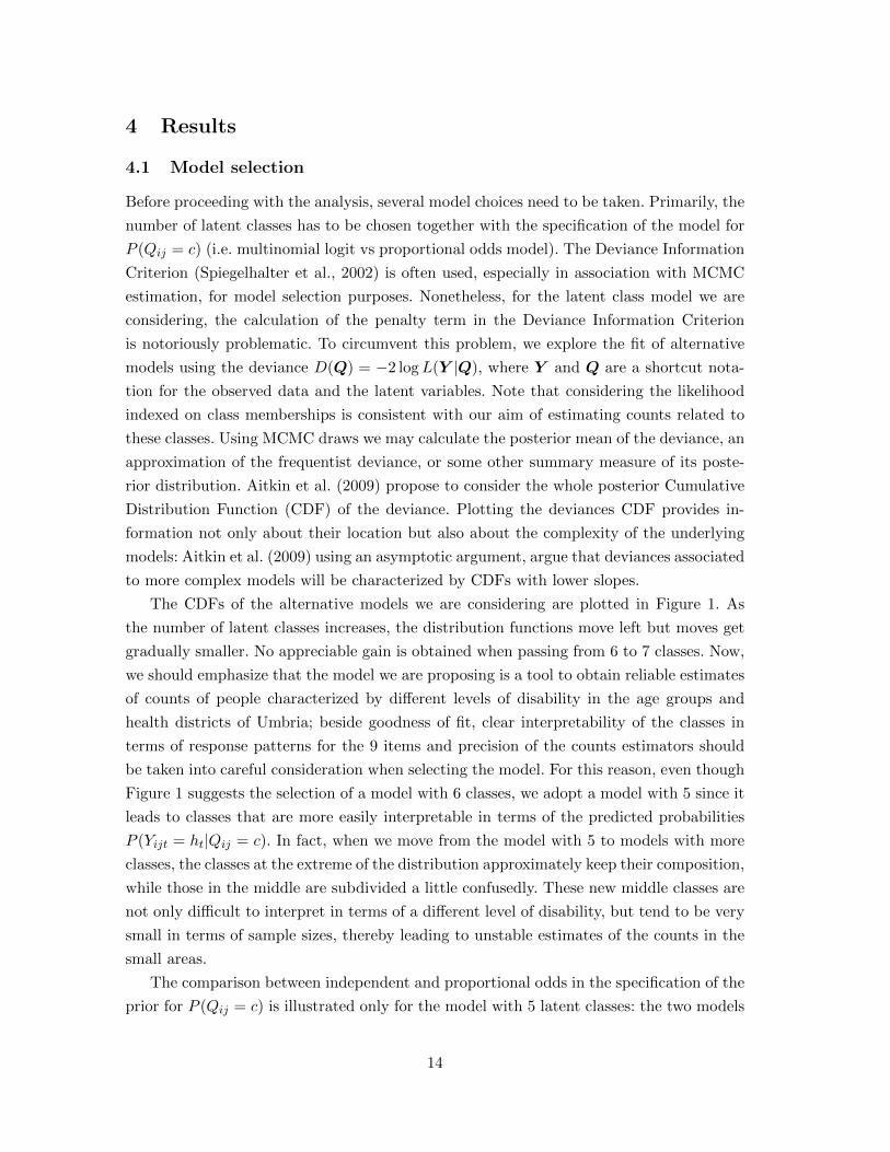
The CDFs of the alternative models we are considering are plotted in Figure 1. As

the number of latent classes increases, the distribution functions move left but moves get

gradually smaller. No appreciable gain is obtained when passing from 6 to 7 classes. Now,

we should emphasize that the model we are proposing is a tool to obtain reliable estimates

of counts of people characterized by different levels of disability in the age groups and

health districts of Umbria; beside goodness of fit, clear interpretability of the classes in

terms of response patterns for the 9 items and precision of the counts estimators should

be taken into careful consideration when selecting the model. For this reason, even though

Figure 1 suggests the selection of a model with 6 classes, we adopt a model with 5 since it

leads to classes that are more easily interpretable in terms of the predicted probabilities

P (Yijt = ht|Qij = c). In fact, when we move from the model with 5 to models with more

classes, the classes at the extreme of the distribution approximately keep their composition,

while those in the middle are subdivided a little confusedly. These new middle classes are

not only difficult to interpret in terms of a different level of disability, but tend to be very

small in terms of sample sizes, thereby leading to unstable estimates of the counts in the

small areas.

The comparison between independent and proportional odds in the specification of the

prior for P (Qij = c) is illustrated only for the model with 5 latent classes: the two models

14

3600 3800 4000 4200 4400 4600 4800

0.0

0.2

0.4

0.6

0.8

1.0

deviance

EC

DF

3 classes proportional odds

4 classes proportional odds

5 classes proportional odds

6 classes proportional odds

7 classes proportional odds

5 classes independent odds

Figure 1: Deviances’ CDFs associated to alternative models.

15

perform very closely and similar evidences may be obtained for models with a different

number of latent classes. For this reason we consider the more parsimonious proportional

odds model.

We also exclude from the chosen model the ‘marital status’ covariate as in all models

it gives no appreciable contribution to the improvement of the fit and the associated slope

parameters have diffuse posterior distributions centered approximately around 0. Finally,

note that the number and placement of the knots for the p-spline approximation of the

effect of age has been kept fixed in all models. In particular, 12 knots have been used

and chosen to be placed at the quantiles of the distribution of age (recall that we are

considering only people aged 50 or more and we have 50 unique values of age).

4.2 Model checking and sensitivity analysis

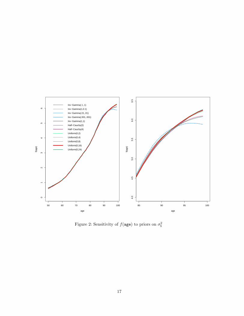
In this section we illustrate a sensitivity analysis exercise to assess the impact of the

selected prior distributions and parameters on the estimates of interest. Let’s focus first

on the prior for σ2b , a parameter that rules the smoothness of the p-spline of equation (3).

The sensitivity exercise is also useful to motivate the choice of the prior for σ2b introduced

in Section 3.3. Recall that we have selected a proportional odds model for the probability

of belonging to a latent class, and therefore we have a single function for the effect of age

and a single σ2b , instead of the σ2bc.

We consider three popular classes of priors: i) the Inv-Gamma(a, b) for σ2b ; ii) the

Uniform(0, B) on σb and iii) the Half-Cauchy(S) on σb. See Gelman (2006) for motivation

and details about these priors for variance components. For all the three classes of priors we

consider different sets of values for their parameters. A graphical evaluation of the impact

that the considered priors have on the posterior expectation of f(age) in (3) is shown in

Figure 2. As expected, regardless of the chosen distribution, the more diffuse is the prior,

the more curved is the p-spline. Nonetheless, because of the large sample size, this effect

is weak except for the extreme ages (for which we have fewer observations). Also in this

part of the plot most priors lead to almost identical curves and observed differences have

no impact on classification of individuals with respect to disability. The only exception is

represented by Inv-Gamma(a, b) with ‘small’ parameters.

The Half-Cauchy(S) priors have not been considered in estimation since they slow

down the MCMC computations with respect to other available options. We decide to use

the Uniform(0, B) priors as they show little sensitivity to the choice of B, at least in the

range we consider. The value B = 16 is chosen as it is ‘large’ with respect to the size of the

effects (as suggested in the literature) but not so extreme to produce a too curved spline.

Similar sensitivity exercises have been conducted also for the variance component σ2vfrom which it emerges that the posterior distributions of the districts effect are largely

unaffected by the choice of the prior among those we have considered. The same prior

16

50 60 70 80 90 100

01

23

45

6

age

f(ag

e)

Inv−Gamma(.1,.1)

Inv−Gamma(1,0.1)

Inv−Gamma(.01,.01)

Inv−Gamma(.001,.001)

Inv−Gamma(1,1)

Half−Cauchy(2)

Half−Cauchy(4)

Uniform(0,2)

Uniform(0,4)

Uniform(0,8)

Uniform(0,16)

Uniform(0,24)

85 90 95 100

4.0

4.5

5.0

5.5

6.0

6.5

age

f(ag

e)

Figure 2: Sensitivity of f(age) to priors on σ2b

17

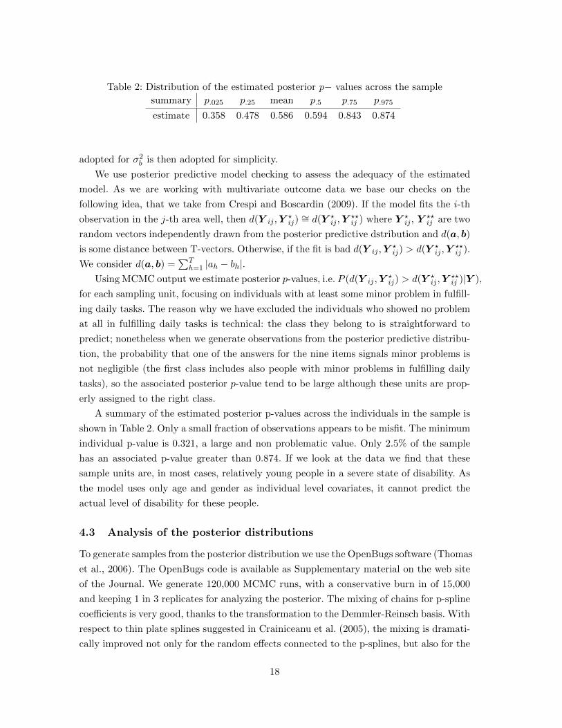
Table 2: Distribution of the estimated posterior p− values across the sample

summary p.025 p.25 mean p.5 p.75 p.975

estimate 0.358 0.478 0.586 0.594 0.843 0.874

adopted for σ2b is then adopted for simplicity.

We use posterior predictive model checking to assess the adequacy of the estimated

model. As we are working with multivariate outcome data we base our checks on the

following idea, that we take from Crespi and Boscardin (2009). If the model fits the i-th

observation in the j-th area well, then d(Y ij ,Y?ij)∼= d(Y ?

ij ,Y??ij ) where Y ?

ij , Y??ij are two

random vectors independently drawn from the posterior predictive dstribution and d(a, b)

is some distance between T-vectors. Otherwise, if the fit is bad d(Y ij ,Y?ij) > d(Y ?

ij ,Y??ij ).

We consider d(a, b) =∑T

h=1 |ah − bh|.Using MCMC output we estimate posterior p-values, i.e. P (d(Y ij ,Y

?ij) > d(Y ?

ij ,Y??ij )|Y ),

for each sampling unit, focusing on individuals with at least some minor problem in fulfill-

ing daily tasks. The reason why we have excluded the individuals who showed no problem

at all in fulfilling daily tasks is technical: the class they belong to is straightforward to

predict; nonetheless when we generate observations from the posterior predictive distribu-

tion, the probability that one of the answers for the nine items signals minor problems is

not negligible (the first class includes also people with minor problems in fulfilling daily

tasks), so the associated posterior p-value tend to be large although these units are prop-

erly assigned to the right class.

A summary of the estimated posterior p-values across the individuals in the sample is

shown in Table 2. Only a small fraction of observations appears to be misfit. The minimum

individual p-value is 0.321, a large and non problematic value. Only 2.5% of the sample

has an associated p-value greater than 0.874. If we look at the data we find that these

sample units are, in most cases, relatively young people in a severe state of disability. As

the model uses only age and gender as individual level covariates, it cannot predict the

actual level of disability for these people.

4.3 Analysis of the posterior distributions

To generate samples from the posterior distribution we use the OpenBugs software (Thomas

et al., 2006). The OpenBugs code is available as Supplementary material on the web site

of the Journal. We generate 120,000 MCMC runs, with a conservative burn in of 15,000

and keeping 1 in 3 replicates for analyzing the posterior. The mixing of chains for p-spline

coefficients is very good, thanks to the transformation to the Demmler-Reinsch basis. With

respect to thin plate splines suggested in Crainiceanu et al. (2005), the mixing is dramati-

cally improved not only for the random effects connected to the p-splines, but also for the

18

20000 30000 40000 50000 60000

3540

4550

5560

Trace of beta, Deimmler−Reinsch basis spline

Iterations

20000 30000 40000 50000 60000

12

34

5

Trace of beta, thin plate spline

Iterations

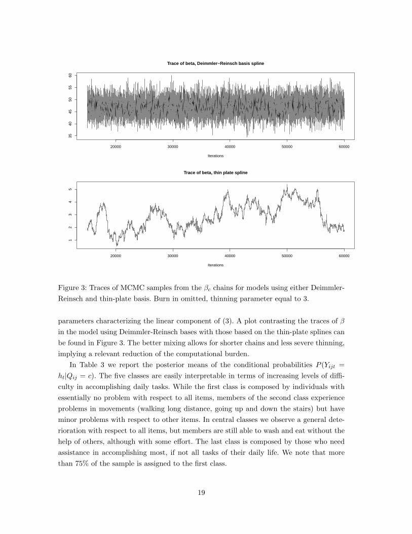
Figure 3: Traces of MCMC samples from the βc chains for models using either Deimmler-

Reinsch and thin-plate basis. Burn in omitted, thinning parameter equal to 3.

parameters characterizing the linear component of (3). A plot contrasting the traces of β

in the model using Deimmler-Reinsch bases with those based on the thin-plate splines can

be found in Figure 3. The better mixing allows for shorter chains and less severe thinning,

implying a relevant reduction of the computational burden.

In Table 3 we report the posterior means of the conditional probabilities P (Yijt =

ht|Qij = c). The five classes are easily interpretable in terms of increasing levels of diffi-

culty in accomplishing daily tasks. While the first class is composed by individuals with

essentially no problem with respect to all items, members of the second class experience

problems in movements (walking long distance, going up and down the stairs) but have

minor problems with respect to other items. In central classes we observe a general dete-

rioration with respect to all items, but members are still able to wash and eat without the

help of others, although with some effort. The last class is composed by those who need

assistance in accomplishing most, if not all tasks of their daily life. We note that more

than 75% of the sample is assigned to the first class.

19

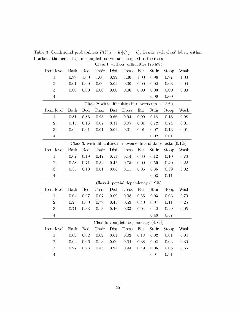
Table 3: Conditional probabilities P (Yijt = ht|Qij = c). Beside each class’ label, within

brackets, the percentage of sampled individuals assigned to the class

Class 1: without difficulties (75.8%)

Item level Bath Bed Chair Dist Dress Eat Stair Stoop Wash

1 0.99 1.00 1.00 0.99 1.00 1.00 0.98 0.97 1.00

2 0.01 0.00 0.00 0.01 0.00 0.00 0.02 0.03 0.00

3 0.00 0.00 0.00 0.00 0.00 0.00 0.00 0.00 0.00

4 0.00 0.00

Class 2: with difficulties in movements (11.5%)

Item level Bath Bed Chair Dist Dress Eat Stair Stoop Wash

1 0.81 0.83 0.93 0.66 0.94 0.99 0.18 0.13 0.98

2 0.15 0.16 0.07 0.33 0.05 0.01 0.72 0.74 0.01

3 0.04 0.01 0.01 0.01 0.01 0.01 0.07 0.13 0.01

4 0.02 0.01

Class 3: with difficulties in movements and daily tasks (6.1%)

Item level Bath Bed Chair Dist Dress Eat Stair Stoop Wash

1 0.07 0.19 0.47 0.53 0.14 0.86 0.12 0.10 0.76

2 0.58 0.71 0.52 0.42 0.75 0.09 0.50 0.40 0.22

3 0.35 0.10 0.01 0.06 0.11 0.05 0.35 0.39 0.02

4 0.03 0.11

Class 4: partial dependency (1.9%)

Item level Bath Bed Chair Dist Dress Eat Stair Stoop Wash

1 0.04 0.07 0.07 0.09 0.08 0.56 0.03 0.03 0.70

2 0.25 0.60 0.79 0.45 0.59 0.40 0.07 0.11 0.25

3 0.71 0.33 0.13 0.46 0.33 0.04 0.42 0.29 0.05

4 0.48 0.57

Class 5: complete dependency (4.8%)

Item level Bath Bed Chair Dist Dress Eat Stair Stoop Wash

1 0.02 0.02 0.02 0.03 0.02 0.13 0.02 0.01 0.04

2 0.02 0.06 0.13 0.06 0.04 0.38 0.02 0.02 0.30

3 0.97 0.93 0.85 0.91 0.94 0.49 0.06 0.05 0.66

4 0.91 0.91

20

50 60 70 80 90 100

02

46

8

age

f(ag

e)

Figure 4: The posterior meanf(age) (black line) with a 95% probability interval (grey

area) based on 0.025 and 0.975 posterior quantiles

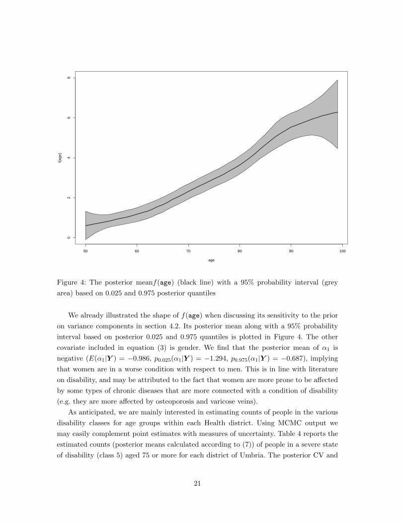
We already illustrated the shape of f(age) when discussing its sensitivity to the prior

on variance components in section 4.2. Its posterior mean along with a 95% probability

interval based on posterior 0.025 and 0.975 quantiles is plotted in Figure 4. The other

covariate included in equation (3) is gender. We find that the posterior mean of α1 is

negative (E(α1|Y ) = −0.986, p0.025(α1|Y ) = −1.294, p0.975(α1|Y ) = −0.687), implying

that women are in a worse condition with respect to men. This is in line with literature

on disability, and may be attributed to the fact that women are more prone to be affected

by some types of chronic diseases that are more connected with a condition of disability

(e.g. they are more affected by osteoporosis and varicose veins).

As anticipated, we are mainly interested in estimating counts of people in the various

disability classes for age groups within each Health district. Using MCMC output we

may easily complement point estimates with measures of uncertainty. Table 4 reports the

estimated counts (posterior means calculated according to (7)) of people in a severe state

of disability (class 5) aged 75 or more for each district of Umbria. The posterior CV and

21

50 60 70 80 90 100

0.0

0.1

0.2

0.3

0.4

0.5

age

pfem

ales

.pg.

cl5$

mea

n

Perugino district class 5

Valnerina district class 5

Perugino district class 4

Valnerina district class 4

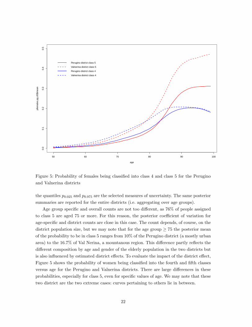
Figure 5: Probability of females being classified into class 4 and class 5 for the Perugino

and Valnerina districts

the quantiles p0.025 and p0.975 are the selected measures of uncertainty. The same posterior

summaries are reported for the entire districts (i.e. aggregating over age groups).

Age group specific and overall counts are not too different, as 76% of people assigned

to class 5 are aged 75 or more. For this reason, the posterior coefficient of variation for

age-specific and district counts are close in this case. The count depends, of course, on the

district population size, but we may note that for the age group ≥ 75 the posterior mean

of the probability to be in class 5 ranges from 10% of the Perugino district (a mostly urban

area) to the 16.7% of Val Nerina, a mountanous region. This difference partly reflects the

different composition by age and gender of the elderly population in the two districts but

is also influenced by estimated district effects. To evaluate the impact of the district effect,

Figure 5 shows the probability of women being classified into the fourth and fifth classes

versus age for the Perugino and Valnerina districts. There are large differences in these

probabilities, especially for class 5, even for specific values of age. We may note that these

two district are the two extreme cases: curves pertaining to others lie in between.

22

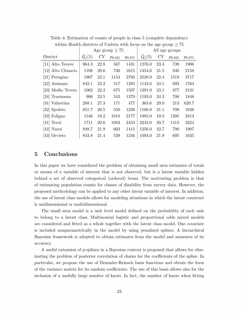
Table 4: Estimation of counts of people in class 5 (complete dependency

within Health districts of Umbria with focus on the age group ≥ 75

Age group ≥ 75 All age groups

District Qj(5) CV p0.025 p0.975 Qj(5) CV p0.025 p0.975

[11] Alto Tevere 964.3 22.8 567 1431 1276.0 23.4 739 1906

[12] Alto Chiascio 1108 20.6 730 1615 1454.0 21.5 946 2158

[21] Perugino 1907 22.1 1154 2793 2528.0 22.4 1519 3717

[22] Assisano 842.1 23.2 517 1285 1142.0 24.1 693 1764

[23] Medio Tevere 1062 22.2 675 1597 1391.0 23.1 877 2131

[24] Trasimeno 906 23.5 543 1379 1193.0 24.3 706 1848

[31] Valnerina 288.1 27.3 171 477 363.6 29.0 213 620.7

[32] Spoleto 851.7 20.5 550 1236 1106.0 21.1 709 1626

[33] Foligno 1546 19.2 1018 2177 1985.0 19.5 1295 2813

[41] Terni 1711 20.6 1083 2453 2242.0 20.7 1412 3224

[42] Narni 948.7 21.9 603 1415 1256.0 22.7 790 1907

[43] Orvieto 843.8 21.4 539 1246 1093.0 21.9 695 1635

5 Conclusions

In this paper we have considered the problem of obtaining small area estimates of totals

or means of a variable of interest that is not observed, but is a latent variable hidden

behind a set of observed categorical (ordered) items. The motivating problem is that

of estimating population counts for classes of disability from survey data. However, the

proposed methodology can be applied to any other latent variable of interest. In addition,

the use of latent class models allows for modeling situations in which the latent construct

is unidimensional or multidimensional.

The small area model is a unit level model defined on the probability of each unit

to belong to a latent class. Multinomial logistic and proportional odds mixed models

are considered and fitted as a whole together with the latent class model. One covariate

is included nonparametrically in the model by using penalized splines. A hierarchical

Bayesian framework is adopted to obtain estimates from the model and measures of its

accuracy.

A useful extension of p-splines in a Bayesian context is proposed that allows for elim-

inating the problem of posterior correlation of chains for the coefficients of the spline. In

particular, we propose the use of Demmler-Reinsch basis functions and obtain the form

of the variance matrix for its random coefficients. The use of this basis allows also for the

inclusion of a usefully large number of knots. In fact, the number of knots when fitting

23

p-splines with MCMC methods is usually kept very low to avoid numerical instabilities.

This extension can be recommended any time p-splines are fitted using MCMC methods,

also within simpler nonparametric regression models.

References

Agresti, A. (2002). Categorical Data Analysis. John Wiley & Sons.

Aitkin, M., C. Liu, and T. Chadwick (2009). Bayesian model comparison and model

averaging for small-area estimation. The Annals of Applied Statistics 3, 199–221.

Cabrero-Garcıa, J. and J. A. Lopez-Pina (2008). Aggregated measures of functional dis-

ability in a nationally representative sample of disabled people: analysis of dimensional-

ity according to gender and severity of disability. Quality of Life Research 17, 425–436.

Crainiceanu, C., D. Ruppert, and M. P. Wand (2005). Bayesian analysis for penalized

spline regression using winbugs. Journal of Statistical Software 14.

Crespi, C. and W. Boscardin (2009). Bayesian model checking for multivariate outcome

data. Computational Statistics and Data Analysis 53, 3765–3772.

Eilers, P. H. C. and B. D. Marx (1996). Flexible smoothing with B-splines and penalties.

Statistical Science 11 (2), 89–121.

Erosheva, E. A. (2002). Grade of Membership and Latent Structure Models With Appli-

cation to Disability Survey Data. Phd Dissertation: Department of Statistics, Carnegie

Mellon University, Pittsburgh, PA.

Fabrizi, E. and C. Trivisano (2009). Robust linear mixed models for small area estimation.

Journal of Statistical Planning and Inference 140, 433–443.

Gelman, A. (2006). Prior distributions for variance parameters in hierarchical models.

Bayesian Analysis 1, 515–533.

Ghosh, M., K. Natarajan, T. W. F. Stroud, and C. B. P (1998). Generalized linear models

for small-area estimation. Journal of the American Statistical Association 93, 273–282.

Jiang, J. and P. Lahiri (2006). Mixed model prediction and small area estimation (with

discussion). Test 15, 1–96.

Katz, S., A. B. Ford, R. W. Moskowitz, B. A. Jackson, and M. W. Jaffe (1963). Studies

of illness in the aged. the index of ADL: a standardized measure of biological and psy-

chosocial function. Journal of the American Medical Association 185, 914–919.

Lazarsfeld, P. and N. Henry (1968). Latent structure analysis. Boston, Houghton Mifflin.

Mesbah, M. (2004). Measurement and analysis of health related quality of life and envi-

ronmental data. Envirometrics 15, 473–481.

Montanari, G. E., M. G. Ranalli, and P. Eusebi (2011). Latent variable modeling of

disability in people aged 65 or more. Statistical Methods and Applications 20, 49–63.

Nychka, D. and D. Cummins (1996, MAY). Flexible smoothing with B-splines and penal-

24

ties - Comment. STATISTICAL SCIENCE 11 (2), 104–105.

Opsomer, J. D., G. Claeskens, M. G. Ranalli, G. Kauermann, and F. J. Breidt (2008).

Non-parametric small area estimation using penalized spline regression. Journal of the

Royal Statistical Society, Series B: Statistical Methodology 70 (1), 265–286.

Rao, J. (2003). Small Area Estimation. Wiley Series in Survey Methodology.

Ruppert, D., M. P. Wand, and R. J. Carroll (2003). Semiparametric Regression. Cambridge

University Press, Cambridge, New York.

Spiegelhalter, D., N. Best, B. Carlin, and A. van der Linde (2002). Bayesian measures

of model complexity and fit (with discussion). Journal of the Royal Statistical Society,

ser. B 64, 583–639.

Thomas, A., B. O’Hara, U. Ligges, and S. Sturz (2006). Making bugs open. R news 6,

12–17.

25