A GIS-based approach to documenting large canid damage to bones

Palaeogeography, Palaeoclimatology, Palaeoecology 409 (2014) 57–71

Contents lists available at ScienceDirect

Palaeogeography, Palaeoclimatology, Palaeoecology

j ourna l homepage: www.e lsev ie r .com/ locate /pa laeo

A GIS-based approach to documenting large canid damage to bones

Jennifer A. Parkinson a,⁎, Thomas W. Plummer b, Rebecca Bose c

a Department of Anthropology, City University of New York Graduate Center and NYCEP, 365 Fifth Ave., Room 6402, New York, NY 10016, USAb Department of Anthropology, Queens College, City University of New York and NYCEP, 65-30 Kissena Blvd., Flushing, NY 11367, USAc Wolf Conservation Center, P.O. Box 421, South Salem, NY 10590, USA

⁎ Corresponding author.E-mail addresses: [email protected] (J.A. Parkinson

[email protected] (T.W. Plummer).

http://dx.doi.org/10.1016/j.palaeo.2014.04.0190031-0182/© 2014 Elsevier B.V. All rights reserved.

a b s t r a c t
a r t i c l e i n f o
Article history:Received 8 October 2013Received in revised form 21 April 2014Accepted 30 April 2014Available online 9 May 2014

Keywords:TaphonomyBone surface modificationFeeding experimentsCanids

Experimental studies of modern carnivore tooth marking patterns are integral to understanding the nature ofcarnivore involvement in archeological bone assemblages. However, modern bone damage data for mostcarnivore taxa are limited. This is particularly true for canids. This study presents bone damage data collectedfrom feeding experiments conducted with Mexican Gray Wolves (Canis lupus baileyi) and Red Wolves (Canisrufus). This is the largest experimental assemblage reported for canids to date. The image-analysis GIS approachdescribed by Marean et al. (2001) is expanded on here and used to document bone preservation and tooth markdistribution for the first time in a carnivore-modified bone assemblage. Further, we introduce the use of the ArcGISSpatial Analyst to identify significant concentrations of bone modifications. Results show that the distribution oftooth pits varies considerably across elements as well as across different portions of the same element, and thatsignificant clusters of tooth pits occur on all long bones.We suggest thatwith a large enough sample, the GIS SpatialAnalyst can be a useful tool for analyzing the distribution of bonemodifications with greater resolution than previ-ous methods. This method facilitates comparisons between experimental and fossil assemblages which may aid inidentifying the timing of access to carcasses by carnivores involved inmodifying fossil assemblages. Finally, the useof this rigorous methodology is a step toward increasing standardization in methods of taphonomic analysis.

© 2014 Elsevier B.V. All rights reserved.

1. Introduction

Bone damage patterns created on prey animals bymodern carnivorescan be used as a proxy to interpret the involvement of extinct carnivoresin archeological bone assemblages. This question has been particularlypertinent to researchers interested not only in carnivore behavior, butalso in assessing potential competitive interactions between carnivoresand hominins over the course of human evolution. Unfortunately,modern experimental datasets for carnivore-induced modifications arelimited. This is particularly true for canids, whichwere potentially impor-tant agents of bone modification and assemblage formation during thePlio-Pleistocene of Eurasia, North America and Africa.

Taphonomic studies of carnivore bone modification have paidparticular attention to patterns produced by hyaenids (Blumenschine,1988; Marean and Spencer, 1991; Marean et al., 1992; Blumenschineand Marean, 1993; Capaldo, 1997; Faith, 2007; Kuhn et al., 2009) andfelids (Domínguez-Rodrigo, 1999; Domínguez-Rodrigo and Barba,2006; Pobiner, 2007; Gidna et al., 2013) in African settings. However,little attention has been paid to the bone modification signature oflarge canids. Canids were an important part of the Pleistocene largecarnivoran paleoguild, and somewere potentially high-level competitors

),

(Brugal and Boudadi-Maligne, 2011). Although large canid fossils overlapwith modern and pre-modern human archeological occurrences, thedegree to which large canids may have competed with and influencedfood acquisition behaviors of pre-modern humans is notwell understood.

This study presents newbone damage data from feeding experimentsconducted with large canids. A GIS image analysis method is used torecord and analyze bone preservation patterns and surface modificationsin the experimental assemblage. Thismethod, developed byMarean et al.(2001), provides a powerful means of analyzing and archiving largeamounts of bone fragment data. Using the GIS image-analysis methodhas several advantages. 1) It allows for more accurate recording andbetter visual representation of bone surface modifications, which can beexamined relative to the degree of preservation of particular elementportions. 2) The powerful relational database function of ArcGIS softwareprovides a means of organizing and analyzing data on a finer scale thanwould otherwise be possible, including damage density and the spatialrelationship of damage to anatomical markers. 3) This approach canprovide a means of standardizing zooarcheological data collectionmethods.

1.1. Pleistocene large canid distribution

Canids are abundant and taxonomically diverse throughout thePlio-Pleistocene record of Europe (Brugal and Boudadi-Maligne,2011). Large canids appear in the Western European record just below

http://crossmark.crossref.org/dialog/?doi=10.1016/j.palaeo.2014.04.019&domain=pdf

http://dx.doi.org/10.1016/j.palaeo.2014.04.019

mailto:[email protected]

mailto:[email protected]


http://www.sciencedirect.com/science/journal/00310182

0.0

AG

E (

MA

)

NO

RT

H A

ME

RIC

AN

EP

OC

H

0.4

PLE

IST

OC

EN

E

0.2

0.6

0.8

1.0

1.2

1.4

1.6

1.8

2.0

Ear

lyM

iddl

eLa

.P

LIO

CE

NE

Ranc

hola

brea

nIr

vin

gto

nia

nB

lancan

Arrows indicate chronospecies. Dotted line indicates insecure record.Age ranges for species based on the following: C. dirus (Dundas 1999); C. lupus, Cuon, C. etruscus, C. mosbachensis (Brugal & Boudadi-Maligne 2011); C. chihliensis (Tong et al. 2012); X. falconeri; X. lycanoides, L. pictus (Martínez-Navarro & Rook 2003); L. sekowei (Hartsone-Rose et al. 2010)

EURASIAN. AMERICA

2.2

2.4

Late

AFRICA

Villa

franchia

nG

ale

ria

n

LAN

D M

AM

MA

L A

GE

EU

RO

PE

AN

LAN

D M

AM

MA

L A

GE

Cuo

n

Can

is d

irus

Can

is lu

pus

Xen

ocyo

n

Lyca

on p

ictu

s

Can

is e

trus

cus

Can

is m

osba

chen

sis

Xen

ocyo

n (=

Lyca

on)

lyca

noid

es

Lyca

on s

ekow

ei

(=Ly

caon

) fa

lcon

eri?

Can

is c

hihl

iens

is

Fig. 1. Distribution of large canid species during the Late Pliocene and Pleistocene. Data from Dundas (1999); Brugal and Boudadi-Maligne (2011); Tong et al. (2012); Martínez-Navarroand Rook (2003); Hartsone-Rose et al. (2010).

Fig. 2.Mexican GrayWolves at theWolf Conservation Center during feeding experiments.Photo credit: Spencer Wilhelm.

58 J.A. Parkinson et al. / Palaeogeography, Palaeoclimatology, Palaeoecology 409 (2014) 57–71

the Plio-Pleistocene boundary at around 2.0 Ma, following thewell-known European faunal turnover ‘wolf-event’ (Azzaroli, 1983;Torre et al., 1992). This turnover is marked by a major extinction ofcarnivores in Europe, including the cursorial hyaenid Chasmaportheteslunensis, the appearance of the large hyaenid Pachycrocuta brevirostris,and a radiation of large canid species (Martínez-Navarro and Rook,2003; Sardella and Palombo, 2007).

Some of the earliest canids in Europe that potentially overlap pre-modern humans are thewolf-like Canis etruscus and Canismosbachensis(Fig. 1). Although their taxonomy is disputed, these species arepotentially a single lineage that persisted from the Early through theMiddle Pleistocene. The modern Canis lupus lineage appears in the LatePleistocene (Brugal and Boudadi-Maligne, 2011). Dental morphometricanalyses show that the slicing component of the C. lupus dentition ismore developed than the crushing component, suggesting that wolveshave a more carnivorous diet than these earlier species of Canis (Brugaland Boudadi-Maligne, 2011).

Two other genera of large, hyper-carnivorous (flesh specialist) canidsare present in Pleistocene Eurasia: Cuon (the Asiatic wild dog) andXenocyon, which some consider to be the same genus as the African hunt-ing dog (Lycaon) (Martínez-Navarro and Rook, 2003). The genusXenocyon includes two chronospecies: Xenocyon (=Lycaon) falconeriand Xenocyon (=Lycaon) lyconoides, which persisted in Eurasia untiltheMiddle Pleistocene (Martínez-Navarro and Rook, 2003). These earlierspecies of lycaon-like canids were larger in size than extant Africanhunting dogs and more comparable to modern wolves, with hyper-carnivorous dental morphology (Martínez-Navarro and Rook, 2003).

The African fossil record of canids is comparatively small. The earliestlarger-sized canids (i.e., larger than jackal-sized) from Africa are knownfrom Ain Hanech, Algeria (1.8 Ma) (Sahnouni et al., 2002), and alsofrom Kromdraai Member A (ca. 1.5 Ma) (Turner, 1986; Geraads, 2011),Sterkfontein Valley Coopers D (1.6–1.9 Ma) and Gladysvale (1.0 Ma)(Hartstone-Rose et al., 2010), and Olduvai Beds I (ca. 1.84) and II (ca.1.75–1.20) (Ewer, 1965). These African species have been publishedunder various names (Canis atrox, Canis africanus), but they likely

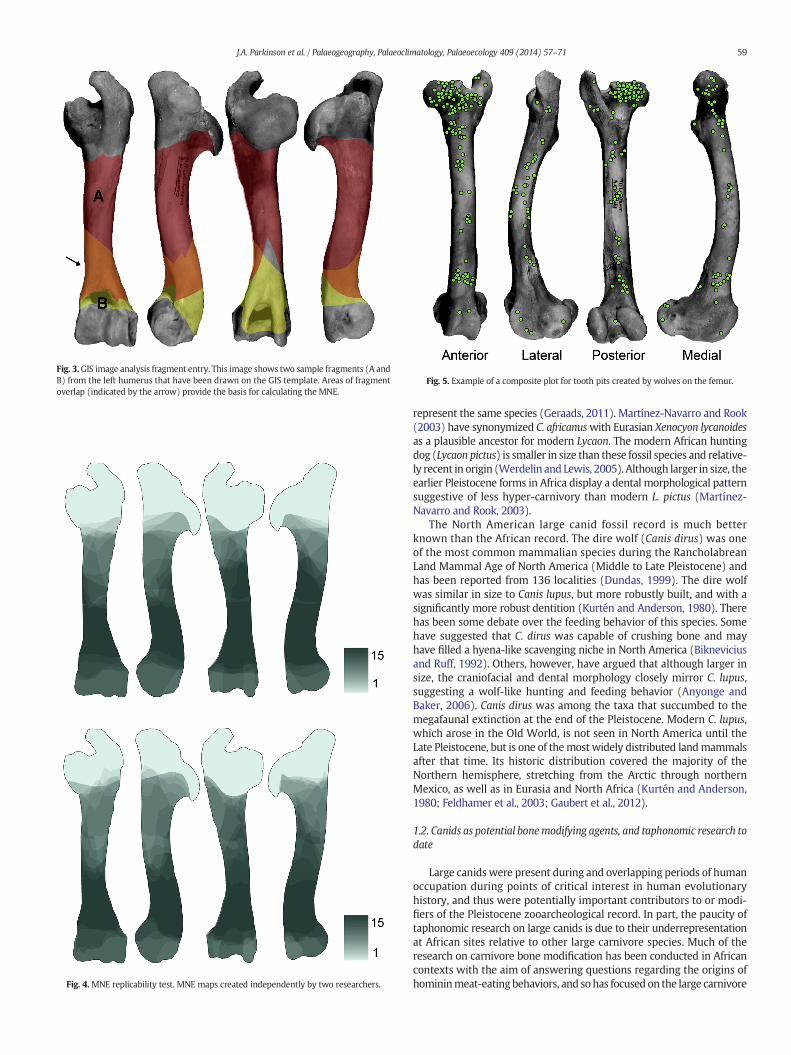
Fig. 3.GIS image analysis fragment entry. This image shows two sample fragments (A andB) from the left humerus that have been drawn on the GIS template. Areas of fragmentoverlap (indicated by the arrow) provide the basis for calculating the MNE.

Fig. 4.MNE replicability test. MNE maps created independently by two researchers.

Fig. 5. Example of a composite plot for tooth pits created by wolves on the femur.

59J.A. Parkinson et al. / Palaeogeography, Palaeoclimatology, Palaeoecology 409 (2014) 57–71

represent the same species (Geraads, 2011). Martínez-Navarro and Rook(2003) have synonymized C. africanuswith Eurasian Xenocyon lycanoidesas a plausible ancestor for modern Lycaon. The modern African huntingdog (Lycaon pictus) is smaller in size than these fossil species and relative-ly recent in origin (Werdelin and Lewis, 2005). Although larger in size, theearlier Pleistocene forms in Africa display a dental morphological patternsuggestive of less hyper-carnivory than modern L. pictus (Martínez-Navarro and Rook, 2003).

The North American large canid fossil record is much betterknown than the African record. The dire wolf (Canis dirus) was oneof the most common mammalian species during the RancholabreanLand Mammal Age of North America (Middle to Late Pleistocene) andhas been reported from 136 localities (Dundas, 1999). The dire wolfwas similar in size to Canis lupus, but more robustly built, and with asignificantly more robust dentition (Kurtén and Anderson, 1980). Therehas been some debate over the feeding behavior of this species. Somehave suggested that C. dirus was capable of crushing bone and mayhave filled a hyena-like scavenging niche in North America (Bikneviciusand Ruff, 1992). Others, however, have argued that although larger insize, the craniofacial and dental morphology closely mirror C. lupus,suggesting a wolf-like hunting and feeding behavior (Anyonge andBaker, 2006). Canis dirus was among the taxa that succumbed to themegafaunal extinction at the end of the Pleistocene. Modern C. lupus,which arose in the Old World, is not seen in North America until theLate Pleistocene, but is one of themost widely distributed landmammalsafter that time. Its historic distribution covered the majority of theNorthern hemisphere, stretching from the Arctic through northernMexico, as well as in Eurasia and North Africa (Kurtén and Anderson,1980; Feldhamer et al., 2003; Gaubert et al., 2012).

1.2. Canids as potential bonemodifying agents, and taphonomic research todate

Large canids were present during and overlapping periods of humanoccupation during points of critical interest in human evolutionaryhistory, and thus were potentially important contributors to or modi-fiers of the Pleistocene zooarcheological record. In part, the paucity oftaphonomic research on large canids is due to their underrepresentationat African sites relative to other large carnivore species. Much of theresearch on carnivore bone modification has been conducted in Africancontexts with the aim of answering questions regarding the origins ofhomininmeat-eating behaviors, and sohas focused on the large carnivore

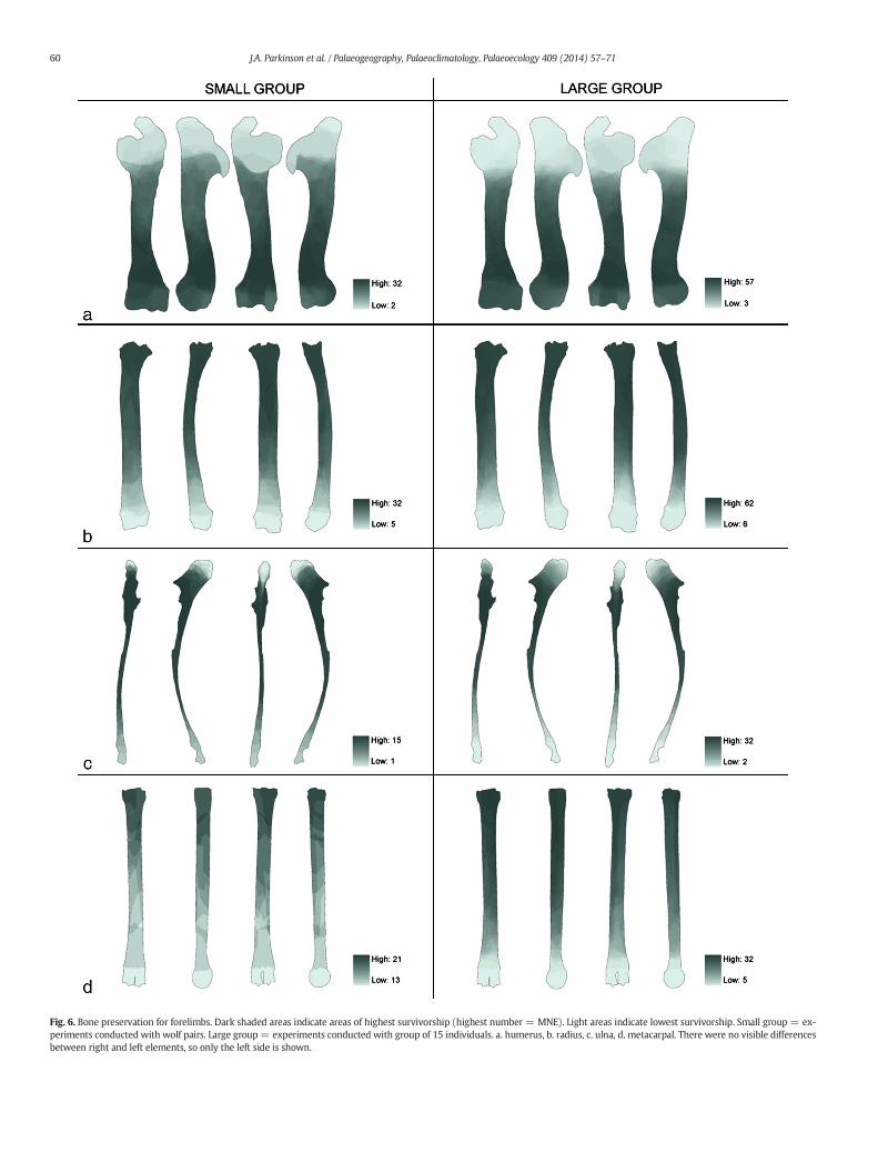
Fig. 6. Bone preservation for forelimbs. Dark shaded areas indicate areas of highest survivorship (highest number = MNE). Light areas indicate lowest survivorship. Small group = ex-periments conducted with wolf pairs. Large group= experiments conducted with group of 15 individuals. a. humerus, b. radius, c. ulna, d. metacarpal. There were no visible differencesbetween right and left elements, so only the left side is shown.


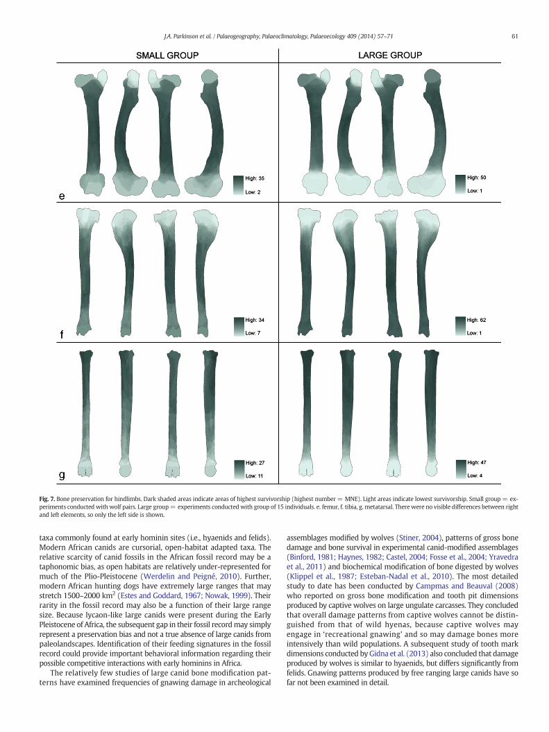
Fig. 7. Bone preservation for hindlimbs. Dark shaded areas indicate areas of highest survivorship (highest number = MNE). Light areas indicate lowest survivorship. Small group = ex-periments conducted with wolf pairs. Large group= experiments conducted with group of 15 individuals. e. femur, f. tibia, g. metatarsal. There were no visible differences between rightand left elements, so only the left side is shown.


taxa commonly found at early hominin sites (i.e., hyaenids and felids).Modern African canids are cursorial, open-habitat adapted taxa. Therelative scarcity of canid fossils in the African fossil record may be ataphonomic bias, as open habitats are relatively under-represented formuch of the Plio-Pleistocene (Werdelin and Peigné, 2010). Further,modern African hunting dogs have extremely large ranges that maystretch 1500–2000 km2 (Estes and Goddard, 1967; Nowak, 1999). Theirrarity in the fossil record may also be a function of their large rangesize. Because lycaon-like large canids were present during the EarlyPleistocene of Africa, the subsequent gap in their fossil recordmay simplyrepresent a preservation bias and not a true absence of large canids frompaleolandscapes. Identification of their feeding signatures in the fossilrecord could provide important behavioral information regarding theirpossible competitive interactions with early hominins in Africa.

The relatively few studies of large canid bone modification pat-terns have examined frequencies of gnawing damage in archeological

assemblages modified by wolves (Stiner, 2004), patterns of gross bonedamage and bone survival in experimental canid-modified assemblages(Binford, 1981; Haynes, 1982; Castel, 2004; Fosse et al., 2004; Yravedraet al., 2011) and biochemical modification of bone digested by wolves(Klippel et al., 1987; Esteban-Nadal et al., 2010). The most detailedstudy to date has been conducted by Campmas and Beauval (2008)who reported on gross bone modification and tooth pit dimensionsproduced by captive wolves on large ungulate carcasses. They concludedthat overall damage patterns from captive wolves cannot be distin-guished from that of wild hyenas, because captive wolves mayengage in ‘recreational gnawing’ and so may damage bones moreintensively than wild populations. A subsequent study of tooth markdimensions conducted byGidna et al. (2013) also concluded that damageproduced by wolves is similar to hyaenids, but differs significantly fromfelids. Gnawing patterns produced by free ranging large canids have sofar not been examined in detail.

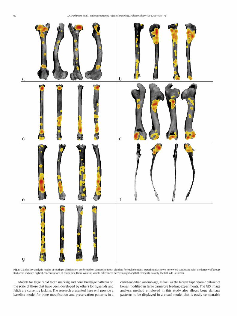
Fig. 8. GIS density analysis results of tooth pit distribution performed on composite tooth pit plots for each element. Experiments shown here were conducted with the large wolf group.Red areas indicate highest concentrations of tooth pits. There were no visible differences between right and left elements, so only the left side is shown.


Models for large canid tooth marking and bone breakage patterns onthe scale of those that have been developed by others for hyaenids andfelids are currently lacking. The research presented here will provide abaseline model for bone modification and preservation patterns in a

canid-modified assemblage, as well as the largest taphonomic dataset ofbones modified in large carnivore feeding experiments. The GIS imageanalysis method employed in this study also allows bone damagepatterns to be displayed in a visual model that is easily comparable

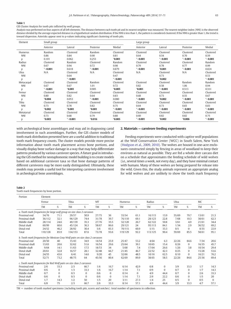
Table 1GIS Cluster Analysis for tooth pits inflicted by wolf groups.Analysiswas performed on four aspects of all left elements. The distance between each tooth pit and its nearest neighbor wasmeasured. The nearest neighbor index (NNI) is the observeddistance divided by the average expected distance in a hypothetical randomdistribution. If theNNI is less than 1, the pattern is considered clustered. If theNNI is greater than 1, the trend istoward dispersion. Asterisks appear next to p-values indicating significant clustering of tooth pits.

Element Small group Large group

Anterior Lateral Posterior Medial Anterior Lateral Posterior Medial

HumerusNNIp

Random0.860.101

Clustered0.840.062

Random0.900.253

Clustered0.81*0.001

Clustered0.64*b0.001




RadiusNNIp


Random0.940.618


Random0.980.879


Clustered0.78*0.001


Random0.990.824

UlnaNNIp

N/A Clustered0.64*b0.001


N/A Clustered0.73*0.002


MetacarpalNNIp


Clustered0.67*0.001

Random1.010.905

Clustered0.72*0.005

Clustered0.82*0.001


Random1.060.513

Random0.940.551

FemurNNIp

Clustered0.80*0.004

Clustered0.820.053


Clustered0.830.080


Clustered0.73*0.002



TibiaNNIp

Clustered0.73*0.002

Clustered0.78*0.001

Clustered0.82*0.001






MetatarsalNNIp

Clustered0.73*0.003


Clustered0.79*0.016

Clustered0.80*0.005


Clustered0.82*0.002

Clustered0.82*0.006



with archeological bone assemblages and may aid in diagnosing canidinvolvement in such assemblages. Further, the GIS cluster models oftoothmark distribution presented here are a useful addition to traditionaltooth mark frequency counts. The cluster models provide more preciseinformation about tooth mark placement across bone portions, andvisually display bone surface damage in away thatmay help differentiatepatterns produced by various carnivore species. A future goal in introduc-ing theGISmethod for neotaphonomicmodel building is to createmodelsbased on additional carnivore taxa so that bone damage patterns ofdifferent carnivores may be more easily distinguished. Ultimately, thesemodels may provide a useful tool for interpreting carnivore involvementin archeological bone assemblages.

Table 2Tooth mark frequencies by bone portion.

Portion Element

Femur Tibia MT

TM % TM % TM %

a. Tooth mark frequencies for large wolf group on size class 2 carcassesProximal end 54/76 71.1 29/57 50.9 27/75 36Proximal shaft 36/112 32.1 96/129 74.4 31/78 39.7Middle shaft 28/114 24.6 49/139 35.3 27/76 35.5Distal shaft 60/99 60.6 45/124 36.3 58/67 86.6Distal end 24/52 46.2 28/92 30.4 5/6 83.3Total 110/128 85.9 134/153 87.6 73/78 93.6

b. Tooth mark frequencies for Mexican Gray Wolf pairs on size class 2 carcassesProximal end 20/50 40 15/43 34.9 14/54 25.9Proximal shaft 13/63 20.6 32/62 51.6 16/54 29.6Middle shaft 9/64 14.1 11/63 17.5 18/53 34Distal shaft 20/61 32.8 16/57 28.1 32/48 66.7Distal end 24/55 43.6 6/41 14.6 9/20 45Total 52/71 73.2 48/75 64 45/56 80.4

c. Tooth mark frequencies for Red Wolf pairs on size class 2 carcassesProximal end 2/6 33.3 2/3 66.7 1/6 16.7Proximal shaft 0/6 0 1/3 33.3 1/6 16.7Middle shaft 0/7 0 0/3 0 0/6 0Distal shaft 0/6 0 0/3 0 0/6 0Distal end 1/7 14.3 1/2 50 1/5 20Total 6/8 75 2/3 66.7 2/6 33.3

TM = number of tooth marked specimens (including tooth pits, scores and notches) /total nu

2. Materials— carnivore feeding experiments

Feeding experiments were conducted with captive wolf populationsat the Wolf Conservation Center (WCC) in South Salem, New York(Hodgson et al., 2009, 2010). The wolves are housed in one-acre enclo-sures constructed simply by fencing in areas of woodland to keep theirenvirons as natural as possible. They are fed a whole deer carcass dieton a schedule that approximates the feeding schedule of wild wolves(i.e., several times aweek, not every day), and they haveminimal contactwith humans. Many of these wolves are being prepared for release intothe wild. Given this, the study animals represent an appropriate analogfor wild wolves and are unlikely to show the tooth mark frequency

Humerus Radius Ulna MC

TM % TM % TM % TM %

33/54 61.1 16/115 13.9 55/69 79.7 13/61 21.376/110 69.1 28/123 22.8 7/68 10.3 38/61 62.332/120 26.7 62/122 50.8 3/61 4.9 21/61 34.429/121 24 95/113 84.1 1/34 2.9 36/52 69.270/115 60.9 5/15 33.3 0/5 0 8/35 22.9

119/129 92.2 113/125 90.4 59/69 85.5 58/61 95.1

25/47 53.2 4/64 6.3 22/26 84.6 7/34 20.625/64 39.1 10/65 15.4 0/26 0 16/35 45.75/68 7.4 17/64 26.6 1/26 3.8 10/34 29.4

21/45 46.7 22/52 42.3 0/25 0 15/28 53.632/66 48.5 10/16 62.5 0/10 0 16/21 76.262/69 89.9 38/65 58.5 22/26 84.6 25/36 69.4

6/14 42.9 0/8 0 3/9 33.3 1/7 14.31/14 7.1 0/9 0 0/7 0 1/7 14.30/14 0 4/9 44.4 0/7 0 2/6 33.31/14 7.1 2/9 22.2 0/6 0 1/5 203/11 27.3 1/4 25 0/5 0 0/5 08/14 57.1 4/9 44.4 3/9 33.3 4/7 57.1

mber of specimens in collection.

Table 3Percentage of total specimens in collection and percentage of midshaft specimens bearing tooth marks.

NISP NISP TM % TM Midshaft NISP Midshaft TM NISP Midshaft % TM

Size 2 carcassesLarge group 743 666 89.6 693 222 32Small Gray Wolf group 398 292 73.4 372 71 19.1Small Red Wolf group 56 29 51.8 52 6 11.5

Size 3 carcassesLarge group 22 17 77.3 22 5 22.7Small Gray Wolf group 5 5 100 5 2 40Small Red Wolf group 3 3 100 3 1 33.3

NISP = number of identifiable specimens.


discrepancies noted between wild and captive carnivores elsewhere(Gidna et al., 2013; Sala et al., 2014).

This study includes bone assemblages produced by three differentgroups of wolves, with the following group composition:

Group 1: Mated pair of Red Wolves (Canis rufus) (weight range24–35 kg.)

Group 2: Mexican GrayWolf pack (Canis lupus baileyi) composed of15 individuals (weight range 26–36 kg.)Group 3: Pair of Mexican Gray Wolf female siblings (weight range26–29 kg.)

Variation in group size provides some information on damageproduced under different competitive regimes. As part of normal wolfprovisioning protocol at WCC, complete deer carcasses were fed towolf groups (Fig. 2). Carcasses were obtained as road kill after WCCstaff were alerted by the New York Department of Transportation. Allcarcasses fall within the bovid size class 2 category of Bunn (1982). Asmaller sample of size class 3 bison limbs donated by a local farm wasalso included in the study. Wolf pairs were fed one carcass at a time,while the large groupwas fed 3 to 4 carcasses at a time. Feeding compe-tition was probably greatest in Group 2, given the larger number ofwolves per carcass relative to Groups 1 and 3. As the wolves could notbe disturbed frequently, bones were collected as part of the normalmaintenance of their enclosures every three months. This was carriedout through systematic surface collection, which could not includesieving due to time constraints. Very small bone fragmentswere probablymissed by this collection protocol, but small fragments are generallydifficult to identify to anatomical part and so would not have beenincluded in the GIS analysis. Bones that wolves may have swallowed,digested, and deposited in scat were also not collected, as other researchhas shown that these are typically vertebral (Esteban-Nadal et al., 2010),and our focus here is on the limb bones. Because most bones had beenexposed to the elements for at least several weeks, they were largelydefleshed prior to collection. Bones were degreased and cleaned of anyremaining tissue by boiling in a mild solution of water and laundrydetergent in the Anthropology Bone Research Laboratory at QueensCollege. All bones in the sample were examined with a 10× hand lensunder oblique light to identify tooth marks. Tooth marks were identifiedbased on published criteria (Binford, 1981; Bunn, 1981; Blumenschineet al., 1996; Domínguez-Rodrigo and Barba, 2006).

3. Methods— GIS image analysis

A GIS image-analysis approach was used to record bone preservationand tooth mark distribution in the study collections. This method wasoriginally developed for analysis of hominin-induced cut marks(Marean et al., 2001; Abe et al., 2002). However, it is well suited todocumenting other types of bone modification as well. This study is thefirst to apply this approach to a carnivore-modified bone assemblage.The approach essentially treats each element as a “map” onto whichthe outline of bone fragments, as well as bone surface modificationsare recorded.

3.1. Bone portion survivorship

This procedure utilizes ArcGIS software alongwith the Spatial Analystextension and is fully described in Marean et al. (2001). Using this meth-od, the outline of each identifiable fragment is digitally drawn as a vectorimage in ArcGIS over a photographic template of a complete bone. Thephoto template allows for accurate drawing of fragments relative to ana-tomical landmarks. Each fragment is drawn as a separate layer, whichconsists of a shape file linked to a table containing specific informationabout that fragment. The spatial coordinate system in ArcGIS allows alarge number of fragment shape files to be superimposed over the ele-ment template, providing the basis for calculating the minimum numberof elements (MNE). The maximum number of fragment overlaps indi-cates the MNE (Fig. 3). This process produces a shaded MNE “map”which is a composite digital record of the size, position, and shape of allidentifiable fragments of a particular element and side, aswell as an accu-rate visual representation of bone portion survivorship (Abe et al.,2002). Marean et al. (2001, supplementary material) have providedtemplates and several ArcView scripts that automate some of the dataentry process. Data entry can also be accomplished without use of thescripts in more recent versions of ArcGIS.

The MNE function in this software is useful for providing a visualrepresentation of which bone portions are frequently deleted bycarnivore consumption, and which portions are more often preserved.Lyman (2008) has argued that because this method calculates MNE byoverlapping pixels in image files that are drawn by hand, it couldpotentially inflateMNE counts if fragments that do not overlap in realityare drawn slightly overlapping. He conducted a trial with a singlestudent participant to test the replicability of fragment shape drawingand accuracy of MNE counts using an experimental bone assemblageof known derivation. The student in this study was able to fairly consis-tently reproduce the shape of fragments, but fragment size and locationon the template varied from trial to trial. This resulted in MNE talliesthat were 0–50% greater than the actual number.

We have conducted additional trials to test replicability of fragmentdrawing between observers, as well as MNE counts based on directcomparisons between specimens. A zooarcheology student intern trainedin the GIS image analysis method as well as the first author (JAP)participated in a replicability study using a subset of our experimentalbone assemblage. Our study also found that fragment shape wasconsistently reproduced, and MNE counts were consistent betweenparticipants. Both observers obtained an MNE of 15 (the actual MNE inthe assemblage was 16), and the MNE map images appear almost indis-tinguishable (Fig. 4). This concordance may reflect the more intensivelevel of training in bone anatomy that the participants in this study hadreceived, relative to the student in Lyman's trial.

Although replicability in fragment drawing and MNE counts usingthe GIS system was consistent between observers in our study, MNEcounts generated using GIS are slightly underestimated in our experi-ments (on average by about 17%) relative to counts generated usingthe traditional overlap approach (as described in Marean et al., 2001).This is likely because skeletal age and other observable features thatmight indicate two fragments are from different individuals are not

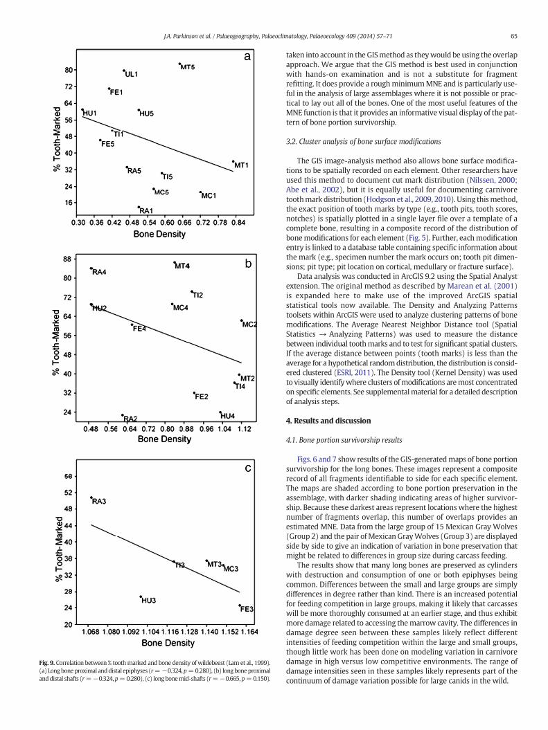
Fig. 9. Correlation between % toothmarked and bone density of wildebeest (Lam et al., 1999).(a) Longboneproximal anddistal epiphyses (r=−0.324,p=0.280), (b) longboneproximalanddistal shafts (r=−0.324,p=0.280), (c) long bonemid-shafts (r=−0.665, p=0.150).


taken into account in the GISmethod as theywould be using the overlapapproach. We argue that the GIS method is best used in conjunctionwith hands-on examination and is not a substitute for fragmentrefitting. It does provide a roughminimumMNE and is particularly use-ful in the analysis of large assemblages where it is not possible or prac-tical to lay out all of the bones. One of the most useful features of theMNE function is that it provides an informative visual display of the pat-tern of bone portion survivorship.

3.2. Cluster analysis of bone surface modifications

The GIS image-analysis method also allows bone surface modifica-tions to be spatially recorded on each element. Other researchers haveused this method to document cut mark distribution (Nilssen, 2000;Abe et al., 2002), but it is equally useful for documenting carnivoretoothmark distribution (Hodgson et al., 2009, 2010). Using thismethod,the exact position of tooth marks by type (e.g., tooth pits, tooth scores,notches) is spatially plotted in a single layer file over a template of acomplete bone, resulting in a composite record of the distribution ofbonemodifications for each element (Fig. 5). Further, eachmodificationentry is linked to a database table containing specific information aboutthe mark (e.g., specimen number the mark occurs on; tooth pit dimen-sions; pit type; pit location on cortical, medullary or fracture surface).

Data analysis was conducted in ArcGIS 9.2 using the Spatial Analystextension. The original method as described by Marean et al. (2001)is expanded here to make use of the improved ArcGIS spatialstatistical tools now available. The Density and Analyzing Patternstoolsets within ArcGIS were used to analyze clustering patterns of bonemodifications. The Average Nearest Neighbor Distance tool (SpatialStatistics → Analyzing Patterns) was used to measure the distancebetween individual toothmarks and to test for significant spatial clusters.If the average distance between points (tooth marks) is less than theaverage for a hypothetical randomdistribution, the distribution is consid-ered clustered (ESRI, 2011). The Density tool (Kernel Density) was usedto visually identifywhere clusters ofmodifications aremost concentratedon specific elements. See supplementalmaterial for a detailed descriptionof analysis steps.

4. Results and discussion

4.1. Bone portion survivorship results

Figs. 6 and 7 show results of the GIS-generatedmaps of bone portionsurvivorship for the long bones. These images represent a compositerecord of all fragments identifiable to side for each specific element.The maps are shaded according to bone portion preservation in theassemblage, with darker shading indicating areas of higher survivor-ship. Because these darkest areas represent locations where the highestnumber of fragments overlap, this number of overlaps provides anestimated MNE. Data from the large group of 15 Mexican Gray Wolves(Group 2) and the pair ofMexican GrayWolves (Group 3) are displayedside by side to give an indication of variation in bone preservation thatmight be related to differences in group size during carcass feeding.

The results show that many long bones are preserved as cylinderswith destruction and consumption of one or both epiphyses beingcommon. Differences between the small and large groups are simplydifferences in degree rather than kind. There is an increased potentialfor feeding competition in large groups, making it likely that carcasseswill be more thoroughly consumed at an earlier stage, and thus exhibitmore damage related to accessing themarrow cavity. The differences indamage degree seen between these samples likely reflect differentintensities of feeding competition within the large and small groups,though little work has been done on modeling variation in carnivoredamage in high versus low competitive environments. The range ofdamage intensities seen in these samples likely represents part of thecontinuum of damage variation possible for large canids in the wild.

1 2 3 4 5Bone Portion

0

20

40

60

80

100

1 2 3 4 5

% T

M

0

20

40

60

80

100

% T

M

0

20

40

60

80

100

% T

M

0

20

40

60

80

100

% T

M

0

20

40

60

80

100

% T

M

0

20

40

60

80

100

% T

M

Bone Portion





Femur Tibia

Humerus Radius

Metacarpal Metatarsal

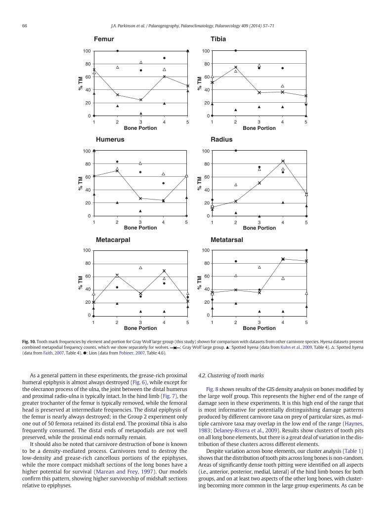
Fig. 10. Toothmark frequencies by element and portion for GrayWolf large group (this study) shown for comparison with datasets from other carnivore species. Hyena datasets presentcombined metapodial frequency counts, which we show separately for wolves. : Gray Wolf large group.▲: Spotted hyena (data from Kuhn et al., 2009, Table 4). Δ: Spotted hyena(data from Faith, 2007, Table 4). ●: Lion (data from Pobiner, 2007, Table 4.6).


As a general pattern in these experiments, the grease-rich proximalhumeral epiphysis is almost always destroyed (Fig. 6), while except forthe olecranon process of the ulna, the joint between the distal humerusand proximal radio-ulna is typically intact. In the hind limb (Fig. 7), thegreater trochanter of the femur is typically removed, while the femoralhead is preserved at intermediate frequencies. The distal epiphysis ofthe femur is nearly always destroyed; in the Group 2 experiment onlyone out of 50 femora retained its distal end. The proximal tibia is alsofrequently consumed. The distal ends of metapodials are not wellpreserved, while the proximal ends normally remain.

It should also be noted that carnivore destruction of bone is knownto be a density-mediated process. Carnivores tend to destroy thelow-density and grease-rich cancellous portions of the epiphyses,while the more compact midshaft sections of the long bones have ahigher potential for survival (Marean and Frey, 1997). Our modelsconfirm this pattern, showing higher survivorship of midshaft sectionsrelative to epiphyses.

4.2. Clustering of tooth marks

Fig. 8 shows results of the GIS density analysis on bones modified bythe large wolf group. This represents the higher end of the range ofdamage seen in these experiments. It is this high end of the range thatis most informative for potentially distinguishing damage patternsproduced by different carnivore taxa on prey of particular sizes, as mul-tiple carnivore taxa may overlap in the low end of the range (Haynes,1983; Delaney-Rivera et al., 2009). Results show clusters of tooth pitson all longbone elements, but there is a great deal of variation in the dis-tribution of these clusters across different elements.

Despite variation across bone elements, our cluster analysis (Table 1)shows that the distribution of tooth pits across long bones is non-random.Areas of significantly dense tooth pitting were identified on all aspects(i.e., anterior, posterior, medial, lateral) of the hind limb bones for bothgroups, and on at least two aspects of the other long bones, with cluster-ing becoming more common in the large group experiments. As can be

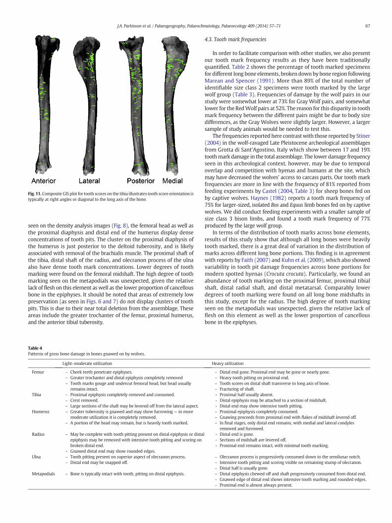
Fig. 11.Composite GIS plot for tooth scores on the tibia illustrates tooth score orientation istypically at right angles or diagonal to the long axis of the bone.


seen on the density analysis images (Fig. 8), the femoral head as well asthe proximal diaphysis and distal end of the humerus display denseconcentrations of tooth pits. The cluster on the proximal diaphysis ofthe humerus is just posterior to the deltoid tuberosity, and is likelyassociated with removal of the brachialis muscle. The proximal shaft ofthe tibia, distal shaft of the radius, and olecranon process of the ulnaalso have dense tooth mark concentrations. Lower degrees of toothmarking were found on the femoral midshaft. The high degree of toothmarking seen on the metapodials was unexpected, given the relativelack of flesh on this element as well as the lower proportion of cancellousbone in the epiphyses. It should be noted that areas of extremely lowpreservation (as seen in Figs. 6 and 7) do not display clusters of toothpits. This is due to their near total deletion from the assemblage. Theseareas include the greater trochanter of the femur, proximal humerus,and the anterior tibial tuberosity.

Table 4Patterns of gross bone damage in bones gnawed on by wolves.

Light–moderate utilization

Femur – Cheek teeth penetrate epiphyses.– Greater trochanter and distal epiphysis completely removed– Tooth marks gouge and undercut femoral head, but head usually

remains intact.Tibia – Proximal epiphysis completely removed and consumed.

– Crest removed.– Large sections of the shaft may be levered off from the lateral aspect.

Humerus – Greater tuberosity is gnawed and may show furrowing — in moremoderate utilization it is completely removed.

– A portion of the head may remain, but is heavily tooth marked.

Radius – May be complete with tooth pitting present on distal epiphysis or distaepiphysis may be removed with intensive tooth pitting and scoring onbroken distal end.

– Gnawed distal end may show rounded edges.Ulna – Tooth pitting present on superior aspect of olecranon process.

– Distal end may be snapped off.

Metapodials – Bone is typically intact with tooth, pitting on distal epiphysis.

4.3. Tooth mark frequencies

In order to facilitate comparison with other studies, we also presentour tooth mark frequency results as they have been traditionallyquantified. Table 2 shows the percentage of tooth marked specimensfor different long bone elements, brokendownbybone region followingMarean and Spencer (1991). More than 89% of the total number ofidentifiable size class 2 specimens were tooth marked by the largewolf group (Table 3). Frequencies of damage by the wolf pairs in ourstudy were somewhat lower at 73% for GrayWolf pairs, and somewhatlower for the RedWolf pairs at 52%. The reason for this disparity in toothmark frequency between the different pairs might be due to body sizedifferences, as the Gray Wolves were slightly larger. However, a largersample of study animals would be needed to test this.

The frequencies reported here contrastwith those reported by Stiner(2004) in the wolf-ravaged Late Pleistocene archeological assemblagesfrom Grotta di Sant'Agostino, Italy which show between 17 and 19%toothmark damage in the total assemblage. The lower damage frequencyseen in this archeological context, however, may be due to temporaloverlap and competition with hyenas and humans at the site, whichmay have decreased the wolves' access to carcass parts. Our tooth markfrequencies are more in line with the frequency of 81% reported fromfeeding experiments by Castel (2004, Table 3) for sheep bones fed onby captive wolves. Haynes (1982) reports a tooth mark frequency of75% for larger-sized, isolated Bos and Equus limb bones fed on by captivewolves. We did conduct feeding experiments with a smaller sample ofsize class 3 bison limbs, and found a tooth mark frequency of 77%produced by the large wolf group.

In terms of the distribution of tooth marks across bone elements,results of this study show that although all long bones were heavilytooth marked, there is a great deal of variation in the distribution ofmarks across different long bone portions. This finding is in agreementwith reports by Faith (2007) and Kuhn et al. (2009), which also showedvariability in tooth pit damage frequencies across bone portions formodern spotted hyenas (Crocuta crocuta). Particularly, we found anabundance of tooth marking on the proximal femur, proximal tibialshaft, distal radial shaft, and distal metatarsal. Comparably lowerdegrees of tooth marking were found on all long bone midshafts inthis study, except for the radius. The high degree of tooth markingseen on the metapodials was unexpected, given the relative lack offlesh on this element as well as the lower proportion of cancellousbone in the epiphyses.

Heavy utilization

– Distal end gone. Proximal end may be gone or nearly gone.– Heavy tooth pitting on proximal end.– Tooth scores on distal shaft transverse to long axis of bone.– Fracturing of shaft.- Proximal half usually absent.- Distal epiphysis may be attached to a section of midshaft.- Distal end may show intensive tooth pitting.– Proximal epiphysis completely consumed.– Gnawing proceeds from proximal end with flakes of midshaft levered off.– In final stages, only distal end remains, with medial and lateral condyles

removed and furrowed.l - Distal end is gone.

- Sections of midshaft are levered off.- Proximal end remains intact, with minimal tooth marking.

– Olecranon process is progressively consumed down to the semilunar notch.– Intensive tooth pitting and scoring visible on remaining stump of olecranon.– Distal half is usually gone.– Distal epiphysis chewed off and shaft progressively consumed from distal end.– Gnawed edge of distal end shows intensive tooth marking and rounded edges.– Proximal end is almost always present.

Fig. 12. Examples of canid damage to size 1 and 2 hind limb bones in this study. A. Range of damage seen on the femora. Posterior view. B. Typical damage to proximal femur. Anterior view(left) and posterior view (right). C. Typical damage tometatarsal. Anterior view. D. Range of damage seen on tibiae. Anterior view. E. Typical damage to the proximal tibia. Anterior tuber-osity gnawed away.


Faith (2007) and Kuhn et al. (2009) have found that elementportionswith lowbone density inmost cases show a reverse correlationwith tooth pit frequency in spotted hyena modified bone assemblages,whereby bone portions with low density are tooth marked at higherfrequencies. This might be expected given that these low density,grease-rich areas are likely of most interest to carnivores. We haveconducted a similar test on our canid modified assemblage to examinethe relationship between tooth mark frequency (from Table 2a: largegroup) and bone density using density data reported for wildebeest byLam et al. (1999) (Fig. 9). Results from our assemblage show a similarnegative but non-significant relationship for proximal and distalepiphyses (r = −0.324, p = 0.280) and for proximal and distal shafts(r=−0.324, p= 0.280). In contrast to Faith's (2007) findings of a slightpositive relationship between tooth mark percentage and bone densityfor hyena modified midshafts, we found a moderate, but non-significantnegative relationship. The stronger, significant negative correlation Faithfound for hyenas in the epiphyses and shaft ends might be expectedgiven that hyenas tend to tooth mark at higher frequencies.

In comparison with tooth mark frequencies reported for othercarnivore taxa (Fig. 10), our canid sample shows on average less

damage than lions (Pobiner, 2007). Given the range of variation intooth mark frequencies reported for spotted hyena assemblages (Faith,2007; Kuhn et al., 2009), it is difficult to distinguish this canid samplefrom hyena modified samples.

4.4. Gross bone damage patterns

Delaney-Rivera et al. (2009) and Pobiner (2007) suggest that toothmark frequencies paired with gross bone destruction patterns mayprovide the best resolution in identifying specific carnivore taxa respon-sible for modifying fossil assemblages. Patterns of gross bone damageare reported here to be considered in conjunctionwith the GIS analysis.

The few studies of large canid taphonomic signatures to date havemainly focused on patterns of gross bone damage. Haynes (1982, 1983)reported modifications to large bovid bones fed on by both wild andcaptive wolves (Canis lupus). The patterns we observed in gross bonedamage in our assemblage of smaller carcasses are largely in agreementwith observations by Haynes. In the most heavily utilized stage, longbones remain either as hollow cylinders, or as cylinders with one end

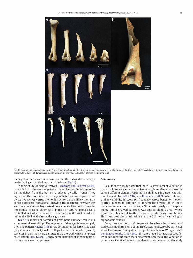
Fig. 13. Examples of canid damage to size 1 and 2 fore limb bones in this study. A. Range of damage seen on the humerus. Posterior view. B. Typical damage to humerus. Note damage toepicondyle. C. Range of damage seen on the radius. Anterior view. D. Range of damage seen on the ulna.


missing. Tooth scores are most common near the ends and occur at rightangles or diagonal to the long axis of the bone (Fig. 11).

In their study of captive wolves, Campmas and Beauval (2008)concluded that the damage pattern that wolves produced cannot bedistinguished from the pattern produced by wild hyenas. Theyargue that the more intense damage inflicted on bones gnawed onby captive wolves versus their wild counterparts is likely the resultof non-nutritional (recreational) gnawing. This difference, however, wasseen only on bones of larger-sized prey animals. This underscores theimportance of using either wild animals or captive animals fed acontrolled diet which simulates circumstances in the wild in order toreduce the likelihood of recreational gnawing.

Table 4 summarizes patterns of gross bone damage seen in ourexperimental assemblage. The sequence of damage follows roughlythe same pattern Haynes (1982) has documented for larger size classprey animals fed on by wild wolf packs, but the smaller (size 2)carcasses in our study were damaged more thoroughly in earlier stagesof utilization. Figs. 12 and 13 show some examples of specific types ofdamage seen in our experiments.

5. Summary

Results of this study show that there is a great deal of variation intooth mark frequencies among different long bone elements as well asamong different element portions. This finding is in agreement withrecent reports by Faith (2007) and Kuhn et al. (2009), which showedsimilar variability in tooth pit frequency across bones for modernspotted hyenas. In addition to documenting variation in toothmark frequencies across bones, a GIS cluster analysis of experi-mental canid-gnawed carcasses was able to identify areas wheresignificant clusters of tooth pits occur on all meaty limb bones.This illustrates the contribution that the GIS method can bring totaphonomic studies.

Comparisons of tooth mark frequencies have been the main focus ofstudies attempting to interpret timing of access to carcasses by carnivoresas well as carcass tissue yield across prehistoric faunas. We agree withDomínguez-Rodrigo (1997, 2002) that there should be increased specific-ity in documenting tooth mark placement. Because of the variation inpatterns we identified across bone elements, we believe that this study


demonstrates the importance of separating analyses by element aswell as bone portion. The GIS image analysis method is particularlywell-suited to examine fine-level variation in tooth marking patternsand may have the potential to differentiate patterns produced by differ-ent carnivore taxa.

5.1. Utility of the GIS image-analysis method

The potential of theGIS spatial statistical tools described in this studyto quantify and analyze bone surface modification patterning providesan improvement on existing methods which also map bone surfacemodifications onto template graphics (e.g., Domínguez-Rodrigo andBarba, 2006; Domínguez-Rodrigo et al., 2007) by allowing for morepowerful statistical analyses. Rather than classifying modifications intoone of several pre-defined zones as other methods have done (e.g.,Marean and Spencer, 1991; Domínguez-Rodrigo, 1999), GIS clusteranalysis identifies important zones based on statistically significantclusters of modifications. Each individual modification can be linkedback to a complete database that contains specific information aboutthe modification as well as information about the fragment on which itoccurs. This method of data storage becomes extremely convenient in alarge assemblage. The database can be queried by any variable includedwithin it (e.g., taxon, size, provenience). Further, because bone surfacemodifications are spatially linked to fragment files, these modificationscan be examined relative to bone portion survival. The spatial linkage ofinformation and powerful analytical tools provided within ArcGIS allowfor numerous andflexible possibilities in theway that data can examined.Using GIS to document bone fragment data can bemore time consumingthan other approaches, but in our experience it is worth this effort for thegreater spatial precision in data recording and greater flexibility in theway research questions can be addressed.

There is great potential for using the GIS image analysis method tobuild models for the interpretation of zooarcheological assemblages.Analyses of modern experimental bone assemblages using this GISmethod can provide valuable analogs with which to compare toothmark and butchery mark distributions in fossil assemblages. While theassemblages in this study model only large canid access, in the futurewe plan to analyze data from assemblages modified by other largecarnivores, as well as humans, in different orders of access. The relation-ship between butchery mark and tooth mark clusters in an archeofaunalassemblage could indicate where differences exist in the type of tissuebeing extracted, and allow for an assessment of variation in carcass usebetween hominins and carnivores. This study serves as a demonstrationof some of the analytical possibilities available with this software. It isour hope that the methodology employed here will encourage greaterstandardization in zooarcheological data recording.

Acknowledgments

We would like to thank the staff of the Wolf ConservationCenter, South Salem, NY for their assistance, especially SpencerWilhelm and Maggie Howell. We also thank student volunteersin the Anthropology Bone Research Laboratory at Queens College(CUNY), Nardai Mootoo, Fotima Askarova and Seema Choudhary,who assisted in cleaning and curating the bone assemblage.Frances Forrest and Claudia Astorino also assisted in collectionof the assemblage. Finally, we thank the editor and anonymousreviewers for their useful comments.

Appendix A. Supplementary material

Supplementary data to this article can be found online at http://dx.doi.org/10.1016/j.palaeo.2014.04.019.

References

Abe, Y., Marean, C.W., Nilssen, P.J., Assefa, Z., Stone, E.C., 2002. The analysis of cutmarks onarchaeofauna: a review and critique of quantification procedures, and a new image-analysis GIS approach. Am. Antiq. 67, 643–663.

Anyonge, W., Baker, A., 2006. Craniofacial morphology and feeding behavior in Canisdirus, the extinct Pleistocene dire wolf. J. Zool. 269, 309–316.

Azzaroli, A., 1983. Quaternary mammals and the “end-villafranchian” dispersal event — aturning point in the history of Eurasia. Palaeogeogr. Palaeoclimatol. Palaeoecol. 44,117–139.

Biknevicius, A.R., Ruff, C.B., 1992. The structure of the mandibular corpus and its relation-ship to feeding behaviours in extant carnivorans. J. Zool. 228 (3), 479–507.

Binford, L.R., 1981. Bones, Ancient Men, Modern Myths. Academic Press, New York.Blumenschine, R.J., 1988. An experimental model of the timing of hominid and carnivore

influence on archaeological bone assemblages. J. Archaeol. Sci. 15, 483–502.Blumenschine, R.J., Marean, C.W., 1993. A carnivore's view of archaeological bone

assemblages. In: Hudson, J. (Ed.), From Bones to Behavior, Ethnoarchaeologicaland Experimental Contributions to the Interpretation of Faunal Remains. Centerfor Archaeological Investigations, University of Southern Illinois, Carbondale,pp. 273–300.

Blumenschine, R.J., Marean, C.W., Capaldo, S.D., 1996. Blind tests of inter-analystcorrespondence and accuracy in the identification of cut marks, percussion marks,and carnivore tooth marks on bone surfaces. J. Archaeol. Sci. 23, 493–507.

Brugal, J., Boudadi-Maligne, M., 2011. Quaternary small to large canids in Europe:taxonomic status and biochronological contribution. Quat. Int. 243, 171–182.

Bunn, H.T., 1981. Archaeological evidence for meat-eating by Plio-Pleistocene hominidsfrom Koobi Fora, Kenya. Nature 291, 574–577.

Bunn, H.T., 1982. Meat-eating and human evolution: studies of the diet and subsistencepatterns of Plio-Pleistocene hominids. (Ph.D. dissertation) , University of California,Berkeley.

Campmas, É., Beauval, C., 2008. Consommation osseuse des carnivores, résultats del'étudede l'exploitation de carcasses de bœufs (Bos taurus) par des loups captifs. Ann.Paléontol. 94, 167–186.

Capaldo, S.D., 1997. Experimental determinations of carcass processing by PlioPleistocenehominids and carnivores at FLK 22 (Zinjanthropus), Olduvai Gorge (Tanzania). J.Hum. Evol. 33, 555–597.

Castel, J.-C., 2004. L'influence des canidés sur la formation des ensembles archéologiques:Caractérisation des destructions dues au loup. Rev. Paléobiol. 23 (2), 675–693.

Delaney-Rivera, C., Plummer, T.W., Hodgson, J.A., Forrest, F., Hertel, F., Oliver, J.S., 2009.Pits and pitfalls, taxonomic variability and patterning in tooth mark dimensions. J.Archaeol. Sci. 36, 2597–2608.

Domínguez-Rodrigo, M., 1997. Meat-eating by early hominids at the FLK 22 Zinjanthropussite, Olduvai Gorge (Tanzania), an experimental approach using cut-mark data. J. Hum.Evol. 33, 669–690.

Domínguez-Rodrigo, M., 1999. Flesh availability and bonemodifications in carcasses con-sumed by lions: palaoecological relevance in hominid foraging patterns. Palaeogeogr.Palaeoclimatol. Palaeoecol. 149, 373–388.

Domínguez-Rodrigo, M., 2002. Hunting and scavenging by early humans, the state of thedebate. J. World Prehist. 16, 1–54.

Domínguez-Rodrigo, M., Barba, R., 2006. New estimates of tooth mark and percussionmark frequencies at the FLK Zinj site, the carnivore-hominid-carnivore hypothesisfalsified. J. Hum. Evol. 50, 170–194.

Domínguez-Rodrigo, M., Barba, R., Egeland, C.P., 2007. Deconstructing Olduvai: ATaphonomic Study of the Bed I Sites. Springer, Dordrecht.

Dundas, R.G., 1999. Quaternary records of the dire wolf, Canis dirus, in North and SouthAmerica. Boreas 28, 375–385.

ESRI, 2011. ArcGIS 9.3 desktop help, spatial analyst. http://webhelp.esri.com/.Esteban-Nadal, M., Cáceres, I., Fosse, P., 2010. Characterization of a current coprogenic

sample originated by Canis lupus as a tool for identifying a taphonomic agent. J.Archaeol. Sci. 37, 2959–2970.

Estes, R.D., Goddard, J., 1967. Prey selection and hunting behavior of the African wild dog.J. Wildl. Manag. 31, 52–70.

Ewer, R.F., 1965. Large Carnivora. In: Leakey, L.S.B. (Ed.), Olduvai Gorge 1951–1961.Cambridge University Press, Cambridge, pp. 19–22.

Faith, J.T., 2007. Sources of variation in carnivore tooth-mark frequencies in amodern spottedhyena (Crocuta crocuta) den assemblage, Amboseli Park, Kenya. J. Archaeol. Sci. 34,1601–1609.

Feldhamer, G.A., Thompson, B.C., Chapman, J.A., 2003. Wild Mammals of NorthAmerica: Biology, Management, and Conservation. Johns Hopkins UniversityPress, Baltimore.

Fosse, P., Laudet, F., Selva, N., Wajrak, A., 2004. Premières observations néotaphonomiquessur des assemblages osseux de Bialowieza (N.E. Pologne): intérêt pour les gisementspléistocènes d'Europe. Paléo 16, 91–116.

Gaubert, P., Bloch, C., Benyacoub, S., Abdelhamid, A., Pagani, P., Djagoun, C., Couloux, A.,Dufour, S., 2012. Reviving the African wolf Canis lupus lupaster in North and WestAfrica: a mitochondrial lineage ranging more than 6000 km wide. PLoS One 7 (8),e42740.

Geraads, D., 2011. A revision of the fossil canidae (Mammalia) of north-western Africa.Palaeontology 54 (2), 429–446.

Gidna, A., Yravedra, J., Domínguez-Rodrigo, M., 2013. A cautionary note on the use ofcaptive carnivores to model wild predator behavior: a comparison of bonemodificationpatterns on long bones by captive and wild lions. J. Archaeol. Sci. 40, 1903–1910.

Hartstone-Rose, A., Werdelin, L., De Ruiter, D.J., Berger, L.R., Churchill, S., 2010. The Plio-Pleistocene ancestor of wild dogs, Lycaon sekowei n. sp. J. Paleontol. 84 (2), 299–308.

Haynes, G., 1982. Utilization and skeletal disturbances of North American prey carcasses.Arctic 35 (2), 266–281.



http://refhub.elsevier.com/S0031-0182(14)00216-8/rf0005





















































http://webhelp.esri.com/






























Haynes, G., 1983. A guide for differentiating mammalian carnivore taxa responsible forgnaw damage to herbivore limb bones. Paleobiology 9, 196-172.

Hodgson, J.A., Plummer, T.W., Forrest, F., Bose, R., Oliver, J., 2009. A GIS-based approach todocumenting large canid damage to bones. PaleoAnthropology A1-A40, A16[abstract].

Hodgson, J.A., Plummer, T.W., Oliver, J.S., Bose, R., 2010. A GIS-based approach todocumenting carnivore and hominin damage to bones. Am. J. Phys. Anthropol. 141(S50), 129 [abstract].

Klippel, W.E., Snyder, L., Parmalee, P., 1987. Taphonomy and archaeologically recoveredmammal bone from southeast Missouri. J. Ethnobiol. 7 (2), 155–169.

Kuhn, B.F., Berger, L.R., Skinner, J.D., 2009. Variation in tooth mark frequencies on longbones from the assemblages of all three extant bone-collecting hyaenids. J. Archaeol.Sci. 36, 297–307.

Kurtén, B., Anderson, E., 1980. Pleistocene Mammals of North America, Columbia UniversityPress, New York.

Lam, Y.M., Chen, X., Pearson, O.M., 1999. Intertaxonomic variability in patterns of bonedensity and the differential representation of bovid, cervid, and equid elements inthe archaeological record. Am. Antiq. 64, 343–362.

Lyman, R.L., 2008. Quantitative Paleozoology, Cambridge University Press, Cambridge.Marean, C.W., Frey, C.J., 1997. Animal bones from caves to cities: reverse utility curves as

methodological artifacts. Am. Antiq. 62, 698–711.Marean, C.W., Spencer, L.M., 1991. Impact of carnivore ravaging on zooarchaeological

measures of element abundance. Am. Antiq. 56, 645–658.Marean, C.W., Spencer, L., Blumenschine, R.J., Capaldo, S., 1992. Zooarchaeological

implications of bone choice and destruction by captive spotted hyenas. J. Archaeol.Sci. 19, 101–121.

Marean, C.W., Abe, Y., Nilssen, P.J., Stone, E.C., 2001. Estimating the minimum number ofskeletal elements (MNE) in zooarchaeology: a review and a new image-analysis GISapproach. Am. Antiq. 66, 333–348.

Martínez-Navarro, B., Rook, L., 2003. Gradual evolution in the African hunting doglineage: systematic implications. Palevol 2, 695–702.

Nilssen, P.J., 2000. An actualistic butchery study in South Africa and its implications forreconstructing hominid strategies of carcass acquisition and butchery in the UpperPleistocene and Plio-Pleistocene. (Ph.D. dissertation) , University of Cape Town.

Nowak, R.M., 1999. Walker's Mammals of the World, vol. 1. Johns Hopkins UniversityPress, Baltimore.

Pobiner, B., 2007. Hominin-carnivore interactions: evidence frommodern carnivore bonemodification and early Pleistocene archaeofaunas (Koobi Fora, Kenya; Olduvai Gorge,Tanzania). (Ph.D. dissertation) Rutgers University.

Sahnouni, M., Hadjouis, D., Van der Made, J., Derradji, A., Canals, A., Medig, M., Belahrech,H., Harichane, Z., Rabhi, M., 2002. Further research at the Oldowan site of Ain Hanech,Northeastern Algeria. J. Hum. Evol. 43, 925–937.

Sala, N., Arsuaga, J.L., Haynes, G., 2014. Taphonomic comparison of bone modificationscaused by wild and captive wolves Canis lupus. Quaternary International 330,126–135.

Sardella, R., Palombo, M.R., 2007. The Pliocene–Pleistocene boundary: which significancefor the so called “Wolf Event”? Evidences from western Europe. Quaternaire 18 (1).

Stiner, M.C., 2004. Comparative ecology and taphonomy of spotted hyenas, humans, andwolves in Pleistocene Italy, 23(2). Revue de Paléobiologie, Genève, pp. 771–785.

Tong, H., Hu, N., Wang, X., 2012. New remains of Canis chihliensis (Mammalia, Carnivora)from Shanshenmiaozui, a Lower Pleistocene site in Yangyuan, Hebei. Vertebrat.PalAsiatic. 50 (4), 335–360.

Torre, D., Ficcarelli, G., Masini, F., Rook, L., Sala, B., 1992. Mammal dispersal events in theearly Pleistocene of western Europe. Cour. Forsch.-Inst. Senckenberg 153, 51–58.

Turner, A., 1986. Miscellaneous carnivore remains from PlioPleistocene deposits in theSterkfontein Valley (Mammalia, Carnivora). Ann. Transv. Mus. 34, 203–226.

Werdelin, L., Lewis, M.E., 2005. Plio-Pleistocene Carnivora of eastern Africa: speciesrichness and turnover patterns. Zool. J. Linnean Soc. 144, 121–144.

Werdelin, L., Peigné, S., 2010. Carnivora. In: Werdelin, L., Sanders, W.J. (Eds.), CenozoicMammals of Africa. University of California Press, Berkely, pp. 609–663.

Yravedra, J., Lagos, L., Bárcena, F., 2011. A taphonomic study of wild wolf (Canis lupus)modification of horse bones in northwestern Spain. J. Taphonomy 9 (1), 37–65.






























































A GIS-based approach to documenting large canid damage to bones

Documents

Transcript of A GIS-based approach to documenting large canid damage to bones