A Gesture Recognition System using Smartphones

Luıs Domingues Tome Jardim Tarrataca

Dissertation for the achievement of the degree

Master in Information Systems and Computer

Engineering

Chairman: Prof. Jose DelgadoSupervisors: Prof. Joao M. P. CardosoAdvisors: Prof. Andreas Wichert

Prof. Pedro Diniz

November 2008

Acknowledgements

A special thanks to Professor Joao Cardoso for providing a real sense of direction to this thesis whetherin the form of ideas, motivation, and experience. Also particularly useful, despite being a time-consuming task, were the annotations and chapter reviews provided. Without his guidance it wouldnot have been possible to accomplish all the objectives set forth.

I would also like to thank Professor Andreas Wichert for all the input provided regarding this masterthesis. His experience in pattern recognition methods and hands-on experience proved to be a valuableresource. Equally important were the advisement given in terms of effort management and businessapplicability considerations.

The best colleague and office mate title belongs to Andre Coelho. Andre helped me scientifically,practically and even emotionally throughout the duration of this master thesis. I would also like tothank other office colleagues such as Bruno Gouveia and Pedro Santos whom by providing feedbackto their own work enabled me to further enhance mine. Thanks for all your useful insights andsuggestions.

Also noteworthy was the support provided by Nokia by funding the research through generous equip-ment donations, namely Nokia’s N80 and N95 smartphones. The equipment provided was crucial inenabling a successful system development. Troy McDaniel from Arizona State University also deservesan acknowledgement for making publicly available his hidden Markov models Java package which en-abled quick application development and testing, allowing me to reap the benefits of previous workand experience.

Finally, a very sincere thank you note to all of those who contributed in a decisive manner to myeducation, regardless of being family, professors or fellow colleagues, my heartfelt gratitute for yourcontribution.

September 1, 2008

i

ii

Abstract

The need to improve communication between humans and computers has been instrumental in definingnew communication models, and new ways of interacting with machines. Humans use gestures in dailylife as a means of communication. The best example of communication through gestures is given bysign languages. With the latest generation of smartphones boasting powerful processors and built-invideo cameras it becomes possible to develop complex and computational expensive applications suchas a gesture recognition system. The goal of this thesis is to present a gesture recognition prototypesystem for smartphones. A model based representation alongside a template based technique weredeveloped for hand posture classification. Comparison between methods evidences the latter superiorrecognition rate. We employed hidden Markov models to model the sequences of hand postures thatform gestures. Hidden Markov models proved to be an efficient tool for dealing with uncertainty dueto their probabilistic nature. We trained a set of gestures and based on user interaction obtained anaverage recognition rate of 83.3%. We concluded that the latest smartphone generation is capableof executing complex image processing applications, with the most penalizing factor being cameraperformance regarding image acquisition rates.

Keywords: Development cycle, hidden Markov models, pattern recognition, skin detection, smart-phone performance, system architecture.

iii

iv

Resumo

A necessidade de melhorar a comunicacao entre seres humanos e computadores tem sido instrumentalpara definir novas modalidades de comunicacao, e novas formas de interagir com maquinas. Os sereshumanos utilizam gestos diariamente como forma de comunicacao. O melhor exemplo de comunicacaoatraves de gestos e representado pelas varias linguagens gestuais existentes. Com a ultima geracao desmartphones a incorporar poderosos processadores e com as camaras de vıdeo incorporadas torna-sepossıvel desenvolver aplicacoes complexas como e o caso dos sistemas de reconhecimento de gestos.O objectivo desta tese consiste no desenvolvimento de um sistema de reconhecimento de gestos paratelemoveis. Por forma a classificar as posturas de mao foram desenvolvidas duas tecnicas, uma baseadaem modelos e outra baseada em templates. O sistema baseado em templates apresentou uma taxa dereconhecimento superior. De forma a modelar as sequencias de posturas que representam os gestosforam utilizados modelos de Markov escondidos. Estes modelos, devido a sua natureza probabilıstica,revelaram-se uma ferramenta eficiente para conseguir lidar com a incerteza que rodeia o processo dereconhecimento de gestos. O sistema final obteve uma taxa media de reconhecimento de 83.3%. Osnossos resultados permitem concluir que a ultima geracao de smarphones e capaz de executar aplicacoesde processamento de imagem complexas. O factor mais penalizador a nıvel de performance do sistemaconsiste nos tempos elevados de captura de imagem das camaras dos dispositivos.

Palavras-chave: Arquitectura de sistema, ciclo de desenvolvimento, desempenho de smartphones,deteccao de pele, modelos de Markov escondidos, reconhecimento de padroes.

v

vi

Contents

List of Figures x

List of Tables xv

List of Acronyms xvii

1 Introduction 1

1.1 Motivation . . . . . . . . . . . . . . . . . . . . . . . . . . . . . . . . . . . . . . . . . . . 11.2 Applications . . . . . . . . . . . . . . . . . . . . . . . . . . . . . . . . . . . . . . . . . . . 31.3 Thesis Goals . . . . . . . . . . . . . . . . . . . . . . . . . . . . . . . . . . . . . . . . . . 41.4 Problem Statement . . . . . . . . . . . . . . . . . . . . . . . . . . . . . . . . . . . . . . . 41.5 Thesis Organization . . . . . . . . . . . . . . . . . . . . . . . . . . . . . . . . . . . . . . 5

2 Skin Detection 7

2.1 Introduction . . . . . . . . . . . . . . . . . . . . . . . . . . . . . . . . . . . . . . . . . . . 72.2 Color and Skin Detection . . . . . . . . . . . . . . . . . . . . . . . . . . . . . . . . . . . 72.3 The Red-Green-Blue basis for color . . . . . . . . . . . . . . . . . . . . . . . . . . . . . . 8

2.3.1 Heuristic Approach . . . . . . . . . . . . . . . . . . . . . . . . . . . . . . . . . . . 92.3.2 Learning Algorithm Approach . . . . . . . . . . . . . . . . . . . . . . . . . . . . . 10

2.4 The Hue-Saturation-Intensity basis for color . . . . . . . . . . . . . . . . . . . . . . . . . 112.5 Metrics . . . . . . . . . . . . . . . . . . . . . . . . . . . . . . . . . . . . . . . . . . . . . 142.6 Background Replacement . . . . . . . . . . . . . . . . . . . . . . . . . . . . . . . . . . . 142.7 Experimental Results . . . . . . . . . . . . . . . . . . . . . . . . . . . . . . . . . . . . . . 162.8 Summary . . . . . . . . . . . . . . . . . . . . . . . . . . . . . . . . . . . . . . . . . . . . 17

3 Posture Recognition 19

3.1 Introduction . . . . . . . . . . . . . . . . . . . . . . . . . . . . . . . . . . . . . . . . . . . 193.2 Convex Hull Approach . . . . . . . . . . . . . . . . . . . . . . . . . . . . . . . . . . . . 20

3.2.1 Convex Hull . . . . . . . . . . . . . . . . . . . . . . . . . . . . . . . . . . . . . . . 203.2.2 Convex Hull applied to Posture Recognition . . . . . . . . . . . . . . . . . . . . 213.2.3 Graham’s Scan . . . . . . . . . . . . . . . . . . . . . . . . . . . . . . . . . . . . . 223.2.4 Clustering Algorithm . . . . . . . . . . . . . . . . . . . . . . . . . . . . . . . . . . 24

3.3 Simple Pattern Recognition Approach . . . . . . . . . . . . . . . . . . . . . . . . . . . . 26

vii

3.4 K Nearest Neighbors Classifier . . . . . . . . . . . . . . . . . . . . . . . . . . . . . . . . 293.4.1 Convex Hull and Euclidean Distance . . . . . . . . . . . . . . . . . . . . . . . . 303.4.2 Simple Pattern Recognition and Hamming Distance . . . . . . . . . . . . . . . . 31

3.5 Experimental Results . . . . . . . . . . . . . . . . . . . . . . . . . . . . . . . . . . . . . 323.5.1 Strategies Developed . . . . . . . . . . . . . . . . . . . . . . . . . . . . . . . . . . 323.5.2 K-Nearest Neighbor and the choice of K . . . . . . . . . . . . . . . . . . . . . . 333.5.3 Interpretation . . . . . . . . . . . . . . . . . . . . . . . . . . . . . . . . . . . . . 34

3.6 Summary . . . . . . . . . . . . . . . . . . . . . . . . . . . . . . . . . . . . . . . . . . . . 36

4 Hidden Markov Models applied to Gesture Recognition 37

4.1 Introduction . . . . . . . . . . . . . . . . . . . . . . . . . . . . . . . . . . . . . . . . . . . 374.2 Discrete Markov Processes . . . . . . . . . . . . . . . . . . . . . . . . . . . . . . . . . . 384.3 Extension to hidden Markov models . . . . . . . . . . . . . . . . . . . . . . . . . . . . . 404.4 The Three Basic Problems for hidden Markov models . . . . . . . . . . . . . . . . . . . 414.5 Solutions to the Problems of hidden Markov models . . . . . . . . . . . . . . . . . . . . 42

4.5.1 Solution to Problem 1 . . . . . . . . . . . . . . . . . . . . . . . . . . . . . . . . . 424.5.2 Solution to Problem 3 . . . . . . . . . . . . . . . . . . . . . . . . . . . . . . . . . 45

4.6 Implementation of hidden Markov models . . . . . . . . . . . . . . . . . . . . . . . . . . 484.7 Experimental Results . . . . . . . . . . . . . . . . . . . . . . . . . . . . . . . . . . . . . . 494.8 Summary . . . . . . . . . . . . . . . . . . . . . . . . . . . . . . . . . . . . . . . . . . . . 50

5 System Implementation 51

5.1 Introduction . . . . . . . . . . . . . . . . . . . . . . . . . . . . . . . . . . . . . . . . . . . 515.2 Smartphone Component . . . . . . . . . . . . . . . . . . . . . . . . . . . . . . . . . . . 525.3 System Architecture . . . . . . . . . . . . . . . . . . . . . . . . . . . . . . . . . . . . . . 54

5.3.1 Development Cycle . . . . . . . . . . . . . . . . . . . . . . . . . . . . . . . . . . 545.3.2 Deployment Model . . . . . . . . . . . . . . . . . . . . . . . . . . . . . . . . . . 56

5.4 Summary . . . . . . . . . . . . . . . . . . . . . . . . . . . . . . . . . . . . . . . . . . . . 60

6 Experimental Results 61

6.1 Introduction . . . . . . . . . . . . . . . . . . . . . . . . . . . . . . . . . . . . . . . . . . . 616.2 Smartphone Performance . . . . . . . . . . . . . . . . . . . . . . . . . . . . . . . . . . . 62

6.2.1 Camera performance . . . . . . . . . . . . . . . . . . . . . . . . . . . . . . . . . 626.2.2 Low-level operations performance . . . . . . . . . . . . . . . . . . . . . . . . . . 636.2.3 System execution time performance . . . . . . . . . . . . . . . . . . . . . . . . . 64

6.3 Profiling . . . . . . . . . . . . . . . . . . . . . . . . . . . . . . . . . . . . . . . . . . . . 656.4 Final system performance . . . . . . . . . . . . . . . . . . . . . . . . . . . . . . . . . . . 67

6.4.1 Experimental Setup . . . . . . . . . . . . . . . . . . . . . . . . . . . . . . . . . . 676.4.2 Results . . . . . . . . . . . . . . . . . . . . . . . . . . . . . . . . . . . . . . . . . 69

6.5 Summary . . . . . . . . . . . . . . . . . . . . . . . . . . . . . . . . . . . . . . . . . . . . 70

7 Conclusions 71

7.1 Future Work . . . . . . . . . . . . . . . . . . . . . . . . . . . . . . . . . . . . . . . . . . 73

viii

7.2 Applications . . . . . . . . . . . . . . . . . . . . . . . . . . . . . . . . . . . . . . . . . . 74

A Lego Mindstorm NXT Component 81

A.1 NXT Middleware . . . . . . . . . . . . . . . . . . . . . . . . . . . . . . . . . . . . . . . . 81A.1.1 Middleware Component Description . . . . . . . . . . . . . . . . . . . . . . . . . 81A.1.2 Usage Example . . . . . . . . . . . . . . . . . . . . . . . . . . . . . . . . . . . . . 82A.1.3 Related Work . . . . . . . . . . . . . . . . . . . . . . . . . . . . . . . . . . . . . . 83

B ARM R©Technology 85

C Application screenshots 89

D Domain Model 91

ix

x

List of Figures

1.1 Alphabet in the American Sign Language (source: [School, 2008]). . . . . . . . . . . . . 2

1.2 System for gesture recognition in human-robot interaction. . . . . . . . . . . . . . . . . 3

1.3 Master thesis organization. . . . . . . . . . . . . . . . . . . . . . . . . . . . . . . . . . . 6

2.1 Rules describing the skin cluster in the RGB color space at uniform daylight illumination. 9

2.2 Rules describing the skin cluster in the RGB color space under flashlight or daylightlateral illumination. . . . . . . . . . . . . . . . . . . . . . . . . . . . . . . . . . . . . . . 10

2.3 Rules describing the skin cluster in the RGB color space under flashlight or daylightlateral illumination. . . . . . . . . . . . . . . . . . . . . . . . . . . . . . . . . . . . . . . 11

2.4 Graphical depiction of HSI. . . . . . . . . . . . . . . . . . . . . . . . . . . . . . . . . . . 12

2.5 The RGB skin locus for figure 2.1. . . . . . . . . . . . . . . . . . . . . . . . . . . . . . . 14

2.6 Exemplification of the background replacement strategy in HSI/RGB skin detection. . 15

2.7 Examples of the different backgrounds. . . . . . . . . . . . . . . . . . . . . . . . . . . . 16

2.8 HSI Results. . . . . . . . . . . . . . . . . . . . . . . . . . . . . . . . . . . . . . . . . . . . 17

2.9 RGB Results. . . . . . . . . . . . . . . . . . . . . . . . . . . . . . . . . . . . . . . . . . . 17

3.1 Classification system diagram: discriminant functions f(x,K) perform some computa-tion on input feature vector x using some knowledge K from training and pass resultsto a final stage that determines the class. . . . . . . . . . . . . . . . . . . . . . . . . . . 20

3.2 Example of a convex hull with a set of points Q = {p0, p1, ..., p12} with its convex hullCH(Q) indicated by the line segments. . . . . . . . . . . . . . . . . . . . . . . . . . . . 21

3.3 Finger extremities of a hand posture in the context of a convex hull. . . . . . . . . . . 21

3.4 Graham’s scan algorithm. . . . . . . . . . . . . . . . . . . . . . . . . . . . . . . . . . . . 23

3.5 Resulting convex hulls applied to two different hand postures. . . . . . . . . . . . . . . 24

3.6 Clustering Algorithm. . . . . . . . . . . . . . . . . . . . . . . . . . . . . . . . . . . . . . 25

3.7 Convex hulls after clustering has been applied to two different hand postures. . . . . . 26

3.8 A row with black cells indicating the presence of skin. . . . . . . . . . . . . . . . . . . . 27

3.9 Encoding Algorithm. . . . . . . . . . . . . . . . . . . . . . . . . . . . . . . . . . . . . . 28

3.10 Two images depicting the transformation process from an image containing a posture(Figure 3.10(a)) to a segmented image with a reduced resolution (Figure 3.10(b)). . . . 28

3.11 K-Nearest Neighbor Algorithm. . . . . . . . . . . . . . . . . . . . . . . . . . . . . . . . 30

3.12 Euclidean distance applied to the convex hull. . . . . . . . . . . . . . . . . . . . . . . . 31

xi

3.13 Hamming distance applied to simple pattern recognition. . . . . . . . . . . . . . . . . . 31

3.14 Different postures used in the experimental results. . . . . . . . . . . . . . . . . . . . . 32

3.15 Average precision results obtained for the black background strategy for different k’s. . 34

3.16 Average precision results obtained for the representative background strategy for differ-ent k’s. . . . . . . . . . . . . . . . . . . . . . . . . . . . . . . . . . . . . . . . . . . . . . 34

3.17 Results obtained for the black background strategy with k = 3. . . . . . . . . . . . . . 35

3.18 Results obtained for the representative background strategy with k = 3. . . . . . . . . . 35

4.1 A Markov chain with 5 states (labeled S1 to S5) with selected state transitions (source:[Rabiner, 1989]). . . . . . . . . . . . . . . . . . . . . . . . . . . . . . . . . . . . . . . . . 39

4.2 Illustration of the sequence of operations required for the computation of the forwardvariable αt+1(j) (source: [Rabiner, 1989]). . . . . . . . . . . . . . . . . . . . . . . . . . 43

4.3 Implementation of the computation of αt(i) in terms of a lattice of observations t, andstates i (source: [Rabiner, 1989]). . . . . . . . . . . . . . . . . . . . . . . . . . . . . . . 44

4.4 Illustration of the sequence of operations required for the computation of the backwardvariable βt(i) (source: [Rabiner, 1989]). . . . . . . . . . . . . . . . . . . . . . . . . . . . 45

4.5 Illustration of the sequence of operations required for the computation of the the jointevent that the system is in state Si at time t and state Sj at time t+ 1. . . . . . . . . 46

4.6 Different hand postures used in the training process of hidden Markov Models. . . . . . 49

5.1 The two smartphones used for system development. . . . . . . . . . . . . . . . . . . . . 53

5.2 Jazelle technology core functional blocks (source:[ARM, 2008a]). . . . . . . . . . . . . . 53

5.3 Development cycle characterization. . . . . . . . . . . . . . . . . . . . . . . . . . . . . . 56

5.4 System Architecture. . . . . . . . . . . . . . . . . . . . . . . . . . . . . . . . . . . . . . 59

6.1 Image acquisition times regarding image resolution. . . . . . . . . . . . . . . . . . . . . 63

6.2 Operation times regarding low-level arithmetic operations. . . . . . . . . . . . . . . . . 64

6.3 Application profiling of the total execution time distribution for Initialization and Exe-cution phases. . . . . . . . . . . . . . . . . . . . . . . . . . . . . . . . . . . . . . . . . . 66

6.4 Profiling of the total execution time distribution for Initialization phase. . . . . . . . . 66

6.5 Profiling of the total execution time distribution for Execution phase. . . . . . . . . . . 67

6.6 Experimental Setup. . . . . . . . . . . . . . . . . . . . . . . . . . . . . . . . . . . . . . 68

6.7 Gesture 1. . . . . . . . . . . . . . . . . . . . . . . . . . . . . . . . . . . . . . . . . . . . 68

6.8 Gesture 2. . . . . . . . . . . . . . . . . . . . . . . . . . . . . . . . . . . . . . . . . . . . 68

6.9 Gesture 3. . . . . . . . . . . . . . . . . . . . . . . . . . . . . . . . . . . . . . . . . . . . 68

6.10 Final system precision results. . . . . . . . . . . . . . . . . . . . . . . . . . . . . . . . . 69

A.1 The interaction process between mobile device and mobile robot. . . . . . . . . . . . . 82

A.2 Middleware interaction example. . . . . . . . . . . . . . . . . . . . . . . . . . . . . . . . 83

B.1 OMAP1710 core functional blocks (source:[TI, 2008a]). . . . . . . . . . . . . . . . . . . 85

B.2 OMAP2420 core functional blocks (source:[TI, 2008b]). . . . . . . . . . . . . . . . . . . 86

B.3 ARM926EJ-S core functional blocks (source:[ARM, 2008c]). . . . . . . . . . . . . . . . 86

xii

B.4 ARM1136JF-S core functional blocks (source:[ARM, 2008b]). . . . . . . . . . . . . . . . 87

C.1 Two sreenshots of the J2SE simulation application developped to test the functionalcores. . . . . . . . . . . . . . . . . . . . . . . . . . . . . . . . . . . . . . . . . . . . . . . 89

C.2 The J2ME application developed. . . . . . . . . . . . . . . . . . . . . . . . . . . . . . . 90

D.1 Higher-level view of the domain model. . . . . . . . . . . . . . . . . . . . . . . . . . . . 91D.2 Domain Model Posture Recognition. . . . . . . . . . . . . . . . . . . . . . . . . . . . . . 92D.3 Domain Model Gesture Recognition. . . . . . . . . . . . . . . . . . . . . . . . . . . . . 93D.4 Domain Model Filters. . . . . . . . . . . . . . . . . . . . . . . . . . . . . . . . . . . . . 94

xiii

xiv

List of Tables

3.1 Encoding obtained for Figure 3.10(b). . . . . . . . . . . . . . . . . . . . . . . . . . . . . 293.2 Execution times. . . . . . . . . . . . . . . . . . . . . . . . . . . . . . . . . . . . . . . . . 33

4.1 Results obtained during the construction and training of hidden Markov models. . . . . 49

6.1 Average execution times per hand posture and maximum FPS. . . . . . . . . . . . . . . 646.2 Mapping between gestures and NXT actions. . . . . . . . . . . . . . . . . . . . . . . . . 68

A.1 Middleware methods list. . . . . . . . . . . . . . . . . . . . . . . . . . . . . . . . . . . . 83

xv

xvi

List of Acronyms

API Application programming interface

ASL American Sign Language

CH Convex Hull

FN False Negatives

FP False Positives

FPS Frames per second

HMM Hidden Markov Model

HSI Hue-Saturation-Intensity

J2ME Java Platform Micro Edition

J2SE Java Standard Edition

JVM Java Virtual Machine

k-NN K-Nearest Neighbor

MIDP Mobile Information Device Profile

MMAPI Mobile Media Application Programming Interface

MVM Multi-tasking Virtual Machine

RGB Red-Green-Blue

TP True Positives

WTK Wireless Toolkit

XML Extensible Markup Language

xvii

Chapter 1

Introduction

1.1 Motivation

Scientists and science fiction writers have been fascinated by the possibility of building intelligentmachines. The capability of understanding the visual world is envisaged for such a machine. Accordingto [Shapiro and Stockman, 2001] Alan Turing, one of the fathers of both the modern digital computerand the field of artificial intelligence, believed that a digital computer would achieve intelligence andthe ability to understand a scene. Such noble goals have proved difficult to achieve and the richnessof human imagination is not yet matched by our engineering.

The need to improve communication between humans and computers has been instrumental in definingnew modalities of communication, and new ways of interacting with machines. Sign language is afrequently used tool when the use of voice is impossible, or when the action of writing and typing isdifficult, but the possibility of vision exists. Moreover, sign language is the most natural and expressiveway for the hearing impaired.

Gestures are thus suited to convey information for which other modalities are not efficient. In naturaland user-friendly interaction, gestures can be used, as a single modality, or combined in multimodalinteraction schemes which involve speech, or textual media. Specification methodologies can be devel-oped to design advanced interaction processes in order to define what kind of gestures are used, whichmeaning they convey, and what the paradigms of interaction are.

Humans use gestures in daily life as a means of communication (e.g., pointing to an object to bringsomeone’s attention to the object, waving ”hello” to a friend, requesting n of something by raising nfingers). The best example of communication through gestures is given by sign languages. Americansign language (ASL) incorporates the entire English alphabet, presented in Figure 1.1, along withmany gestures representing words and phrases, which permits people to exchange information in anonverbal manner.

When it comes to gesture recognition and human-computer interaction there is quite a lot of scien-

1

tific work developed, but before proceeding it is important to distinguish between gesture and pos-ture. This distinction as well as the definition of both terms can be found in [Davis and Shah, 1994],namely:

• Posture - A posture is a specific configuration of hand flexion observed at some time instance;

• Gesture - A gesture is a sequence of postures connected by motions over a short time span.Usually a gesture consists of one or more postures sequentially occurring on the time axis.

Figure 1.1: Alphabet in the American Sign Language (source: [School, 2008]).

A practical example that one can consider where gesture recognition can be applied is in the interactionprocess between humans and robots. A human being can convey information by gestures that wouldotherwise be difficult to transmit. Likewise a robot can also be instructed to interact with humans viagesture recognition, either by a set of gestures configured in advance or by incorporating the ability tolearn new abilities that mimic human gestures and postures.

The feasibility of this interaction process can be studied when one considers human-robot interactionand the abundance of recent smartphones featuring built-in cameras. By developing gesture recognitionsoftware one can transform the camera of a smartphone into a smart camera that effectively becomesthe ”eyes” of a robot providing an input method to the gesture recognition process and thus enablinghuman-robot interaction. Bluetooth technology can enable the communication between smartcameraand robot. Figure 1.2 depicts the system for gesture recognition in human-robot interaction using aNokia N95 smartphone model and a Lego NXT Mindstorms robot.

These factors constitute the main motivations behind this thesis. The focus as well as respective goalsof the work are further explained in section 1.3.

2

Figure 1.2: System for gesture recognition in human-robot interaction.

1.2 Applications

The are many examples for gesture recognition applications. Nintendo’s Wii latest generation console(see [Nintendo, 2008]), has a clear emphasis on increasing interaction levels between video games andtheir human players with a focus on recognizing gestures as input actions.

Authors [King et al., 2005] and [Morrison and McKenna, 2002] also provide another application ofgesture recognition. Physically disabled users, who frequently have trouble providing the strength orprecision necessary to use traditional computer input devices, would also benefit from being able tocontrol devices and enter information via eye blinks, head motions or other gestures.

A number of commercially available products already exist that use gesture recognition as a corecapability in human-computer interaction, namely:

• Canesta’s Virtual Keyboard - [Canesta, 2008] - the virtual keyboard consists of three components:an infrared light source; a pattern projector, which projects the image of a keyboard on a surface,similar to a slide projector; and a sensor, which matches hand and finger movement with thepattern displayed by the pattern projector;

• Cybernet System’s GestureStorm - [Cybernet, 2008a] - for weather map management systemthat utilizes both body tracking and gesture recognition technology to control the computerizedvisual effects;

• Cybernet NaviGaze - [Cybernet, 2008b] - head- and eye-movement based cursor and mouse inter-face technology enables the use of Windows-based computers and applications without a mouse,relying instead on head movement and eye-blinks to control the cursor.

3

1.3 Thesis Goals

The main goals of this thesis focus on the areas of computer vision, pattern recognition and theirapplicability to embedded systems such as smartphones. These goals can be stated as follows:

• Develop algorithms that allow the recognition of hand postures, by utilizing a predefined set ofhand postures;

• Develop algorithms that based on the hand posture recognized allow the recognition of a simplegesture-based language;

• Implement the selected algorithms on a smartphone with a built-in camera in order to commanda robot via Bluetooth technology;

• Study and analyze the capabilities of smartphones to execute computationally intensive algo-rithms;

• Analyze the performance of the algorithms according to their efficiency and processing time;

• Study and analyze the capabilities of smartphones as image acquisition and processing units;

• Study the potential for code optimizations in order to speed-up the performance of the algorithms.

1.4 Problem Statement

Research centered on gesture interaction has provided significant technological improvements, namely[Braffort et al., 1999]:

• Gesture capture and tracking (from video streams or other input devices);

• Motion recognition;

• Motion generation.

In addition, research in the fields of signal processing, pattern recognition, artificial intelligence, andlinguistics is relevant to the areas covered by the multidisciplinary research on gestures as a means ofcommunication.

The recent proliferation of latest generation smartphones featuring advanced capabilities (such as beingable to run operating systems, adding new applications to better serve its users and multimedia featuressuch as video and image capture) has allowed the development of a compact and mobile system withmany features that a few years ago belonged to the realm of a normal computer.

Yet due to their size and battery requirements even today’s most evolved models have constraintsnot usually found on a regular desktop computer. This is especially true when considering that suchdevices are usually resource constrained in both memory and CPU performance. Since sign languageis gesticulated fluently and interactively like other spoken languages, a gesture recognizer must be ableto recognize continuous sign vocabularies and attempt do it in an efficient manner.

4

A vision based approach to gesture recognition can be performed by using the cameras that are includedin most of today’s smartphones and converting them into smart cameras. Smart cameras are camerasthat include image processing algorithms. These algorithms might, for example, extract some featuresof images. In this case the data structures representing feature information are transmitted to the coreof the computational system in order to be properly analyzed. One of the tasks of a smart cameramight be the recognition of gestures identifying a command to be executed and properly notifyingthe system’s core. By developing an approach considering the real-time requirements associated togesture recognition and respective constraints associated to embedded systems, such as smartphones,it becomes possible to study any potential issues that may arise.

1.5 Thesis Organization

This thesis is organized as depicted in Figure 1.3, respectively:

• Chapter 1 - Introduction

Introduces the thesis motivation and presents some existing applications where gesture recogni-tion is a key factor. The goals of the thesis are also presented as well as the problem statementthat supports this work;

• Chapter 2 - Skin Detection

Presents the segmentation process, denominated by ”Skin Detection”. In this process a thresh-olding operation is realized in order to allow for differentiation of background and foreground.This way it becomes possible to label sections of an image as belonging or not to a hand posture;

• Chapter 3 - Posture Recognition

Focuses on feature extraction algorithms that allow the determination of points of interest in aposture. Once the features describing a posture are obtained, they can be compared by a classi-fication algorithm against a labeled database containing features of a sample posture population.The approaches taken toward feature extraction as well as posture classification and respectiveissues are presented in this chapter;

• Chapter 4 - Hidden Markov models applied to gesture recognition

Focuses on the methods developed and respective issues surrounding the use of hidden Markovmodels applied to gesture recognition. Once a posture has been labeled it needs to be contex-tualized with the remaining postures of a gesture in order to provide for semantic meaning in aprobabilistic fashion, this is where the hidden Markov models come into play. The core math-ematical details embodying hidden Markov models as well as main problems and solutions arealso presented in this chapter;

• Chapter 5 - System implementation

Discusses the approach taken towards system implementation namely the development cycle usedas well as core components of the system architecture. The main technological features regarding

5

hardware, software and Java Virtual machine are also discussed in this chapter;

• Chapter 6 - Experimental results

Focuses on the main experimental tests and results performed for the gesture recognition systemdeveloped, such as overall smartphone and system performance.

• Chapter 7 - Conclusions

Concludes this thesis and presents the core conclusions as well as future work points.

Figure 1.3: Master thesis organization.

6

Chapter 2

Skin Detection

2.1 Introduction

Computer vision seeks to build computing techniques that match the process of human vision. Forbetter human-computer interaction it is necessary for machines to recognize various types of interactionsuch as those which are gesture based.

Skin color has proven to be a useful and robust clue for gesture recognition, face detection, local-ization and tracking. The term ”skin color” is not a physical property of an object, rather a per-ceptual phenomenon and therefore a subjective human concept. In the scientific literature severalauthors provide an excellent introductory base for the topic of skin detection and respective issues see[Jones and Rehg, 2002], [Kovac et al., 2003] and [Vezhnevets et al., 2003].

2.2 Color and Skin Detection

Many heuristic and pattern-recognition based strategies have been proposed for achieving robust andaccurate solutions. Among feature-based face detection methods, the ones using skin color as a de-tection cue, have gained large popularity. Color allows for fast processing and experience suggeststhat human skin has a characteristic color, which is easily recognized by humans. The distribu-tion of skin color across different ethnic groups under controlled conditions of illumination has beenshown to be quite compact, with variations expressible in terms of the concentration of skin pigments[Jones and Rehg, 2002]. According to [Kovac et al., 2003] in the right conditions of lighting the sameanalysis can be performed in an efficient manner by computer algorithms.

Other approaches exist that go beyond traditional pattern-recognition based solely on color fundamen-tals. [Zheng et al., 2004] applied statistical skin detection along with the maximum entropy model inorder to determine the presence of adult images. Triesch and Malsburg present an interesting work,see [Triesch and von der Malsburg, 2002], that does not require an initial segmentation of the object

7

from the background. The system presented in this work employs elastic graph matching to determineregions of interest in an image that can later be used for classification.

When color is used as a feature for skin detection it is necessary to choose from a wide range ofpossible color spaces, including RGB , normalized RGB, HSI and YCrCb, among others. Due to it ishuge popularity and wide adoption in the electronics industry, namely digital cameras and computermonitors, the RGB color space presents itself as an adequate candidate to be used in color-based skindetection.

There are however, according to [Vezhnevets et al., 2003], some aspects of the RGB color space thatdo not favor its use, namely the high-correlation between components and the mixing of chrominanceand luminance data. These factors are important when considering the changing nature of color underdifferent illumination conditions. The RGB color space has been used by innumerous authors to studypixel-level skin detection such as [Jones and Rehg, 2002] and [Brand and Mason, 2000].

Due to the different perception of color under uncontrolled light conditions it becomes useful to con-sider other color spaces. The Hue Saturation Intensity is a color model based on human color per-ception with explicit discrimination between luminance and chrominance. This set of properties allowfor interesting properties such as the fact that it is invariant to highlights at white light sources,and also, for matte surfaces, to ambient light and surface orientation relative to the light source[Skarbek and Koschan, 1994]. The explicit discrimination between luminance and chrominance prop-erties of the HSI model presented a strong factor in the choice of a color space as can be seen in the workrelated to skin color segmentation presented in [Zarit et al., 1999] and [Mckenna et al., 1998].

2.3 The Red-Green-Blue basis for color

RGB is a color space originated from CRT display applications, when it was convenient to describecolor as a combination of three colored rays (red, green and blue). It is one of the most widely used colorspaces for processing and storing digital image data such as those acquired by digital cameras.

[Yamaguchi, 1984] provides a detailed analysis of the properties of the RGB color space. The RGBencoding in graphic systems uses one byte for each primary color component (three-byte or 24-bitRGB pixel) enabling

(28)3 or roughly 16 million distinct color encodings. Sensors based on RGB can

distinguish between any pair of different bit encodings, but the encodings may or may not representdifferences that are noticeable in the real world. The encoding of an arbitrary color in the visiblespectrum can be made by combining the encoding of three primary colors - RGB. The amount of eachprimary color gives its intensity. If all components are of highest intensity, then the color white results,equal proportions of less intensity create shades of gray, and finally the color black is represented bythe zeroing of all components.

8

2.3.1 Heuristic Approach

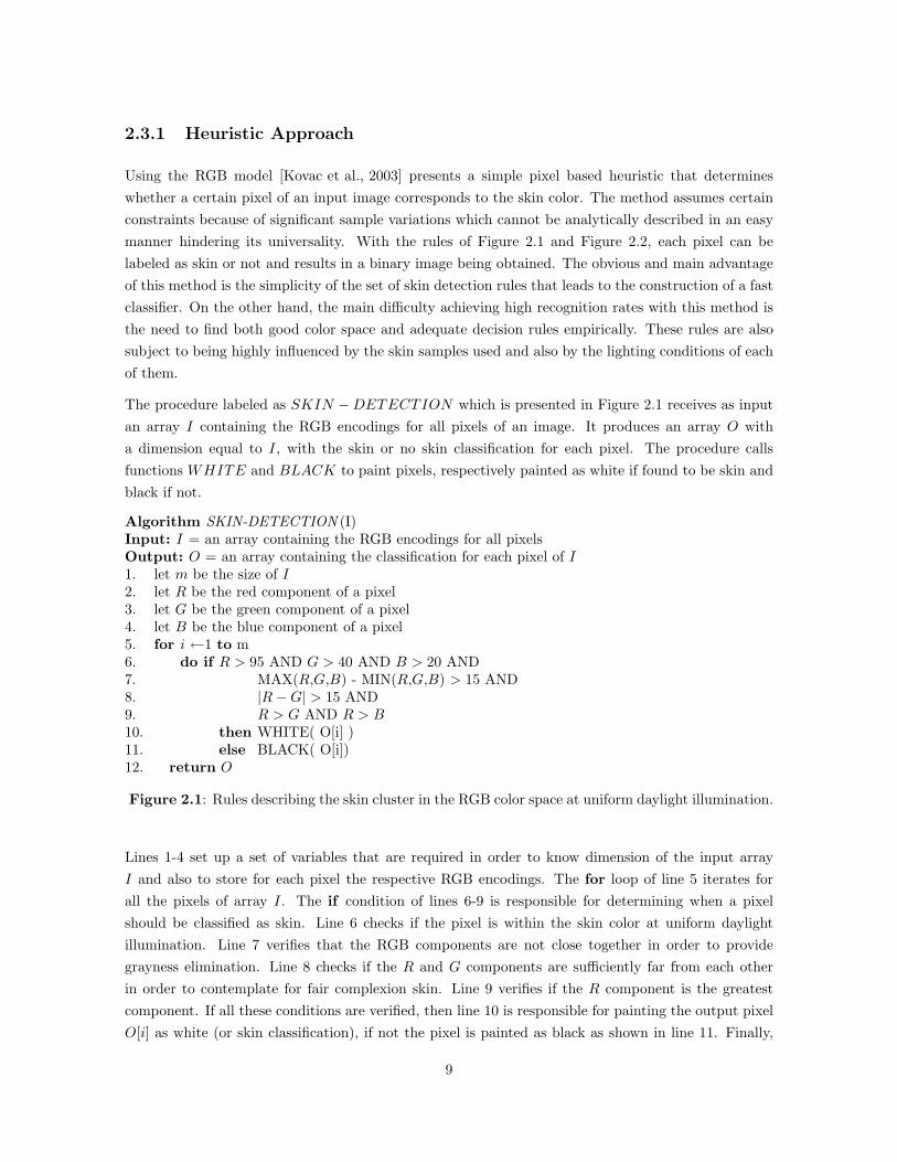
Using the RGB model [Kovac et al., 2003] presents a simple pixel based heuristic that determineswhether a certain pixel of an input image corresponds to the skin color. The method assumes certainconstraints because of significant sample variations which cannot be analytically described in an easymanner hindering its universality. With the rules of Figure 2.1 and Figure 2.2, each pixel can belabeled as skin or not and results in a binary image being obtained. The obvious and main advantageof this method is the simplicity of the set of skin detection rules that leads to the construction of a fastclassifier. On the other hand, the main difficulty achieving high recognition rates with this method isthe need to find both good color space and adequate decision rules empirically. These rules are alsosubject to being highly influenced by the skin samples used and also by the lighting conditions of eachof them.

The procedure labeled as SKIN −DETECTION which is presented in Figure 2.1 receives as inputan array I containing the RGB encodings for all pixels of an image. It produces an array O witha dimension equal to I, with the skin or no skin classification for each pixel. The procedure callsfunctions WHITE and BLACK to paint pixels, respectively painted as white if found to be skin andblack if not.

Algorithm SKIN-DETECTION (I)Input: I = an array containing the RGB encodings for all pixelsOutput: O = an array containing the classification for each pixel of I1. let m be the size of I2. let R be the red component of a pixel3. let G be the green component of a pixel4. let B be the blue component of a pixel5. for i ←1 to m6. do if R > 95 AND G > 40 AND B > 20 AND7. MAX(R,G,B) - MIN(R,G,B) > 15 AND8. |R−G| > 15 AND9. R > G AND R > B10. then WHITE( O[i] )11. else BLACK( O[i])12. return O

Figure 2.1: Rules describing the skin cluster in the RGB color space at uniform daylight illumination.

Lines 1-4 set up a set of variables that are required in order to know dimension of the input arrayI and also to store for each pixel the respective RGB encodings. The for loop of line 5 iterates forall the pixels of array I. The if condition of lines 6-9 is responsible for determining when a pixelshould be classified as skin. Line 6 checks if the pixel is within the skin color at uniform daylightillumination. Line 7 verifies that the RGB components are not close together in order to providegrayness elimination. Line 8 checks if the R and G components are sufficiently far from each otherin order to contemplate for fair complexion skin. Line 9 verifies if the R component is the greatestcomponent. If all these conditions are verified, then line 10 is responsible for painting the output pixelO[i] as white (or skin classification), if not the pixel is painted as black as shown in line 11. Finally,

9

in line 12, the output array O containing the classification for each pixel of I is returned.

Figure 2.2 presents the procedure SKIN − DETECTION which differs from the one presented inFigure 2.1 because it takes into consideration the skin color under flashlight or (light) daylight lateralillumination. It also receives as input an array I containing the RGB encodings for all pixels of animage. It produces an array O with a dimension equal to I, with the skin or no skin classification foreach pixel. The procedure calls functions WHITE and BLACK to paint pixels.

Algorithm SKIN-DETECTION (I)Input: I = an array containing the RGB encodings for all pixelsOutput: O = an array containing the classification for each pixel of I1. let m be the size of I2. let R be the red component of a pixel3. let G be the green component of a pixel4. let B be the blue component of a pixel5. for i ←1 to m6. do if R > 220 AND G > 210 AND B > 170 AND7. |R−G| ≤ 15 AND8. R > B AND G > B9. then WHITE( O[i] )10. else BLACK( O[i])11. return O

Figure 2.2: Rules describing the skin cluster in the RGB color space under flashlight or daylightlateral illumination.

Lines 1-4 set up a set of variables that are required in order to know dimension of the input array I

and also to store for each pixel the respective RGB encodings. The for loop of line 5 iterates for all thepixels of array I. The if condition of lines 6-8 is responsible for determining when a pixel should beclassified as skin. Line 6 checks if the pixel is within the skin color under flashlight or (light) daylightlateral illumination. Line 7 checks if the R and G components are close together. Line 8 verifies if theB component is the smallest component. If this set of conditions is verified, then line 9 is responsiblefor painting the output pixel O[i] as white (or skin classification), if not the pixel is painted as blackas shown in line 10. Finally, in line 11, the output array O containing the classification for each pixelof I is returned.

2.3.2 Learning Algorithm Approach

In the work presented by Gomez and Morales (see [Gomes and Morales, 2002]) a machine learningapproach was proposed to construct a simple rule that enabled fast and efficient skin detection. Theauthors start with three basic color components RGB in a normalized form and apply a learningalgorithm called Restricted Covering Algorithm or RCA, to construct a single rule of no more than asmall number of easy to evaluate terms with a minimum accuracy. It is important to point out thatrepresentativeness of the training set is also an issue, yet the authors algorithm avoids the constructionof too complex decision rules in order to compensate for this situation.

Several decision rules and corresponding terms are obtained, but it is interesting to show (see Figure

10

2.3) the one that the authors evaluation method obtained the highest precision and success raterespectively 91.7% and 92.6% [Gomes and Morales, 2002]. Again the procedure receives as input anarray I containing the RGB encondings for all pixels of an image. It produces an array O witha dimension equal to I, with the skin or no skin classification for each pixel. The procedure callsfunctions WHITE and BLACK to paint pixels.

Algorithm SKIN-DETECTION (I)Input: I = an array containing the RGB encodings for all pixelsOutput: O = an array containing the classification for each pixel of I1. let m be the size of I2. let R be the red component of a pixel3. let G be the green component of a pixel4. let B be the blue component of a pixel5. for i ←1 to m6. do if R/G > 1.185 AND7. R×B

R+G+B2 > 0.107 AND8. R×G

R+G+B2 > 0.1129. then WHITE( O[i] )10. else BLACK( O[i] )11. return O

Figure 2.3: Rules describing the skin cluster in the RGB color space under flashlight or daylightlateral illumination.

Lines 1-4 set up a set of variables that are required in order to know dimension of the input array I

and also to store for each pixel the respective RGB encodings. The for loop of line 5 iterates for allthe pixels of array I. The if condition of lines 6-8 is responsible for determining when a pixel shouldbe classified as skin according to the rule obtained by the authors. If this set of conditions is verified,then line 9 is responsible for painting the output pixel O[i] as white (or skin classification), if not thepixel is painted as black as shown in line 10. Finally, in line 11, the output array O containing theclassification for each pixel of I is returned.

2.4 The Hue-Saturation-Intensity basis for color

In the RGB color space, color codes are highly correlated, and it is impossible to evaluate the similaritiesof two colors from their distance in this space. The mixing of chrominance and luminance data is alsoa disadvantage of the RGB color space.

The HSI system encodes color information by separating an overall intensity value I or L from twovalues encoding chromaticity - hue H and Saturation S.

A color is primarily defined by it chrominance components, namely Hue and Saturation. Hue definesthe dominant color such as red, yellow and blue of an area. Colors with the same hue are distinguishedby their saturation S which refers to the colorfulness of an area in proportion to its brightness. Theintensity component I is related to the color luminance which refers to the amount of light that passesthrough or is emitted from a particular area, and falls within a given solid angle.

11

HSI conceptually represents a double-cone, see Figure 2.4, with white at the top, black at the bottom,and the fully-saturated colors around the edge of a horizontal cross-section with middle gray at itscenter.

Figure 2.4: Graphical depiction of HSI.

Authors Carron and Lambert shows in [Carron and Lambert, 1994] that in color image processing,Hue is closely related to the human perception of colors and that its sensitivity to noise may be lowerthan that of Intensity.

The HSI system is more convenient to some graphic designers because it provides direct control ofbrightness and hue. In addition, the separation of the intensity component in HSI might also providebetter support for computer vision algorithms focusing on the two chromaticity parameters that aremore associated with the color of a surface rather than the source that is lighting it. This situation isparticularly handy to make image processing less sensitive to possible brightness variations ocurringin the working environment.

The luminance component of the color space is in many cases not taken into account in skin detectionapproaches. This decision seems logical, as the goal is to model what can be thought of skin tone, whichis more controlled by the chrominance than luminance coordinates. The dimensionality reduction,achieved by discarding luminance, also simplifies the consequent color analysis. Another argument forignoring luminance is that skin color differs from person to person mostly in brightness and less inthe tone itself. The illumination conditions clearly affect the color of the objects in the scene. Thegoal of any color-based system is diminishing this influence to make color-based recognition robust toillumination change.

However, [Poynton, 1995] points out several undesirable features of these color spaces, including huediscontinuities, and the computation of brightness which conflicts with the properties of color vision.It is also important to refer that if the hardware provides direct support to HSI then the utilization of

12

this color space might be considered. The absence of direct support for the HSI color space requires atransformation process, from the space provided by the hardware to HSI. This situation can potentiallyhamper the use of the HSI model. For instance, due to the fact that most image data in digital camerasis stored in the RGB color space it becomes necessary to conduct an RGB-HSI conversion. TheRGB-HSI conversion presented in 2.1 (see [Gonzalez and Woods, 1992]) can be considered a complexoperation due to the presence of a trigonometric function that is required to obtain the H value.

H = cos−1

23

(r − 1

3

)− 1

3

(b− 1

3

)− 1

3

(g − 1

3

)√23

[(r − 1

3

)2 +(b− 1

3

)2 +(g − 1

3

)2] (2.1)

Equation 2.2 presented in [Swenson, 2002] illustrates a simplified method to obtain the H componentfrom an RGB representation. In this case no trigonometric operation is required.

H =

achromatic if r = g = b

g−b3(r+g−2b) if b = min(r,g,b)

b−r3(g+b−2r) + 1

3 if r = min(r,g,b)r−g

3(r+b−2g) + 23 if g = min(r,g,b)

(2.2)

The components intensity and saturation are easily obtained by equations 2.3 and 2.4

I =r + g + b

3(2.3)

S = 1− 3min(r, g, b) (2.4)

Several authors have presented work (see [Lin and Chen, 1991, Zhang and Wang, 2000]) regarding theuse of HSI in color image segmentation. In this work the segmentation technique used, which ispresented in equation 2.5, only takes into account the Hue component of the HSI color space (as in[Bonato et al., 2005]), allowing for a faster computation and also limiting the amount of computationresources required. In this case H(i, j) represents the Hue values of a certain pixel and T1 and T2

describe inferior and superior thresholds. The thresholds values are required for determining when apixel belongs to a region of interest and they should take into consideration the skin locus on the HSIcolor space. The resulting image contains a binary representation.

f(x, y) =

{1 if T1 <= H(x, y) <= T2

0 otherwise(2.5)

13

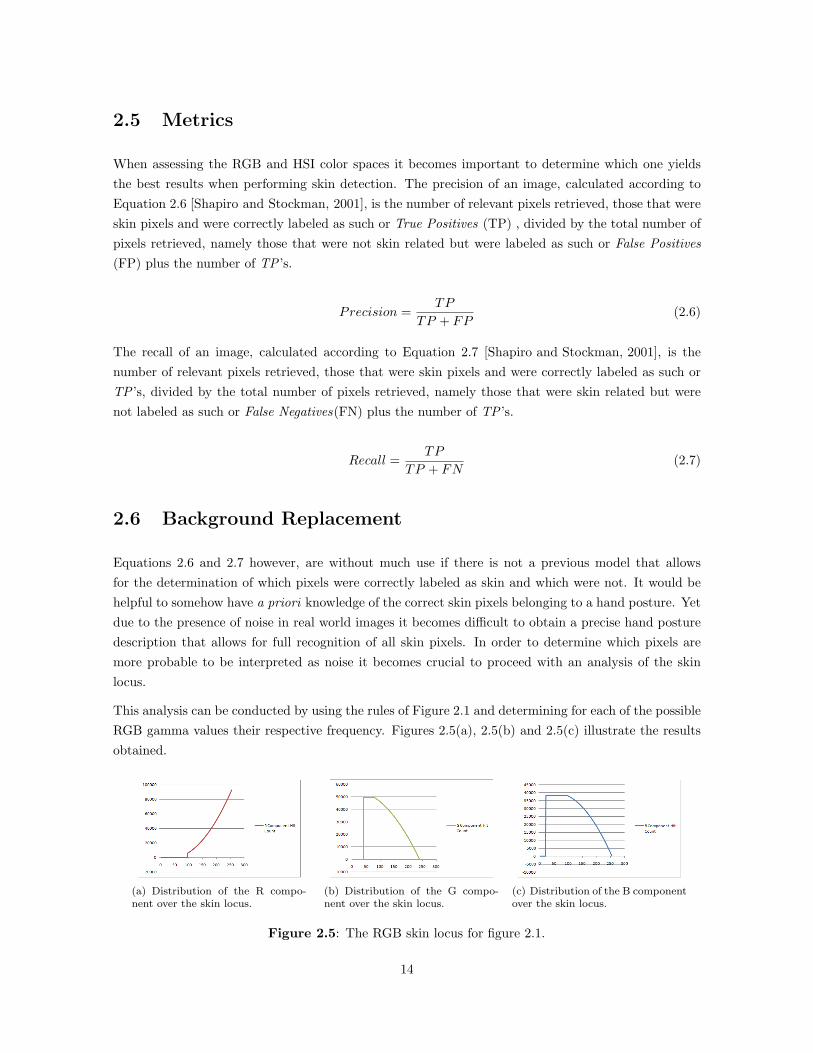
2.5 Metrics

When assessing the RGB and HSI color spaces it becomes important to determine which one yieldsthe best results when performing skin detection. The precision of an image, calculated according toEquation 2.6 [Shapiro and Stockman, 2001], is the number of relevant pixels retrieved, those that wereskin pixels and were correctly labeled as such or True Positives (TP) , divided by the total number ofpixels retrieved, namely those that were not skin related but were labeled as such or False Positives(FP) plus the number of TP ’s.

Precision =TP

TP + FP(2.6)

The recall of an image, calculated according to Equation 2.7 [Shapiro and Stockman, 2001], is thenumber of relevant pixels retrieved, those that were skin pixels and were correctly labeled as such orTP ’s, divided by the total number of pixels retrieved, namely those that were skin related but werenot labeled as such or False Negatives(FN) plus the number of TP ’s.

Recall =TP

TP + FN(2.7)

2.6 Background Replacement

Equations 2.6 and 2.7 however, are without much use if there is not a previous model that allowsfor the determination of which pixels were correctly labeled as skin and which were not. It would behelpful to somehow have a priori knowledge of the correct skin pixels belonging to a hand posture. Yetdue to the presence of noise in real world images it becomes difficult to obtain a precise hand posturedescription that allows for full recognition of all skin pixels. In order to determine which pixels aremore probable to be interpreted as noise it becomes crucial to proceed with an analysis of the skinlocus.

This analysis can be conducted by using the rules of Figure 2.1 and determining for each of the possibleRGB gamma values their respective frequency. Figures 2.5(a), 2.5(b) and 2.5(c) illustrate the resultsobtained.

(a) Distribution of the R compo-nent over the skin locus.

(b) Distribution of the G compo-nent over the skin locus.

(c) Distribution of the B componentover the skin locus.

Figure 2.5: The RGB skin locus for figure 2.1.

14

As can be seen the range of values varies significantly for each component. However, for values ∈ [0, 20]there is no superposition of components allowing for the construction of a background with a colorwhose components have to lie in the same range. This constitutes an ideal background as it avoidsnoise and interference and thus allows for full recognition of skin pixels.

A good candidate for such a background would be a black one that has respectively all of its componentsset to zero. With such a background it is now possible to construct a detailed description of the skinpixels describing a gesture, has there exists a clear contrast between foreground and background. Withthis core image of the gesture description obtained it becomes viable to compare processed images inother backgrounds with the original one and thus obtain a description of the precisions by calculatingequation 2.6.

With such objectives in mind a background replacement strategy was devised in order to substitutethe black background of digital images describing hand postures. By applying this strategy it be-comes feasible to substitute non-skin pixels by those of any background and thus allowing for a largenumber of tests to be realized without incurring significant delays in setting-up the experimental envi-ronment. The process of background replacement is illustrated in figure 2.6(a),2.6(b) and 2.6(c). Anexample of the outputs of skin detection in both HSI and RGB is shown in figures 2.6(d) and 2.6(e),respectively.

(a) The core image describing a pos-ture.

(b) One example of a backgroundimage.

(c) The transformed image combin-ing core with the background.

(d) The HSI processed image withwhite pixels indicating the presenceof skin.

(e) The RGB processed image withwhite pixels indicating the presenceof skin.

Figure 2.6: Exemplification of the background replacement strategy in HSI/RGB skin detection.

15

2.7 Experimental Results

In order to evaluate the performance of the skin detection process in both HSI and RGB color spaces,a total of 17 background images were acquired and combined with 5 core hand postures. Each of thesepostures was represented by 10 images depicting the same posture but with slight variations introducedand related to finger position and spread. The combination of backgrounds with different posturesproduced a total of 850 images that served as input to the different skin detection algorithms.

The RGB color-based skin detection process was based on the rules provided in figure 2.1. As theinput files were all encoded in RGB the HSI color-based method required a transformation which wasdone by applying the rules presented in equation 2.2. After the Hue value had been obtained, equation2.5 was then applied to each pixel in order to determine if it should be labeled or not as skin.

The background images were acquired under normal lighting conditions (i.e., without any auxiliaryillumination that could better lit the scene) during different times of daylight and can be generallyclassified in three classes (Figure 2.7 shows some of those backgrounds):

• Class P - Patio - depicting inner courts open to the sky with an abundance of backgroundobjects (See Figures 2.7(a) and 2.7(b));

• Class G - Garden - depicting scenery in which flower arrangements and vegetation are presentas the majority of background objects (See Figures 2.7(c) and 2.7(d));

• Class C - Corridor - depicting corridors under artificial lighting conditions with an abundanceof background objects (See Figures 2.7(e) and 2.7(f)).

(a) A patio background. (b) A patio background. (c) A garden background. (d) A garden background.

(e) A corridor background. (f) A corridor background.

Figure 2.7: Examples of the different backgrounds.

Figures 2.8 and 2.9 show the average results obtained for recall and precision, respectively R and P forHSI and RGB skin detection methods for the images contained in each class. Also presented are thestandard deviations σR and σP respectively for recall and precision. In all cases there exists reasonablyconsistency across the results.

16

Figure 2.8: HSI Results.

Figure 2.9: RGB Results.

The average recall values for both HSI and RGB remain high and very similar, respectively 99.4% and98.27%. However, there is big discrepancy between the precision values obtained, with the RGB-basedrules presenting an average precision of 82.27% whilst the HSI-based rules obtain an average precisionof 37.83%. In this case it is clearly visible that skin detection rules based on RGB far outperform thevalues obtained by HSI with an average precision increase of 44%. These results favor the use of theRGB color space and rules.

Note however, that both HSI and RGB color-based skin detection may benefit if the parametersof the skin detection rules are tuned to approximate the skin pixels present in a representativedatabase.

Notice also that most digital cameras also operate in the RGB color space and as such the transitionto HSI must be done by software which may impose noticeable execution overhead.

2.8 Summary

We presented in this chapter an introduction to skin detection. Two methods for skin detection basedon the RGB and HSI color spaces and respective consequences were discussed. In order to proceed witha comparative assessment of both methods, two metrics were proposed, namely Recall and Precision.Those two metrics along with a background replacement strategy facilitate the analysis of experimentalresults. The results obtained favor the use of the RGB-based skin detection method.

17

18

Chapter 3

Posture Recognition

3.1 Introduction

In many practical problems, such as posture recognition, there is a need to make some decision aboutthe content of an image or about the classification of an object that it contains. The basic approachtowards object classification views it as a vector of measurements or features. The classification processmight actually fail, either because the posture’s image contains noise, or a new hand posture that thesystem does not know was presented to it.

The model for posture classification followed in this work is an adaptation of the one presented in[Shapiro and Stockman, 2001]. The model contains a set of entities which and can be described asfollows:

• Classes - there is a set of m known classes of objects or postures. These are known either bysome description or by having a set of examples for each of the classes. An ideal class is a setof objects having some important common properties: in practice, a class to which as objectbelongs is denoted by some class label;

• Sample - there is a set of n samples each representing a particular instance of a class;

• Classification - the classification process is responsible for assigning a label to an object ac-cording to some representation of the object’s properties;

• Classifier - is an algorithm that inputs an object representation and outputs a class label. Theclassifier uses the features extracted from the object’s input data to assign it to one of the mdesignated classes C1, C2, ..., Cm;

• Feature Extractor - responsible for extracting information relevant to classification from thedata input and generally producing a vector of features describing the input.

A block diagram of a classification system is given in Figure 3.1. A d-dimensional feature vector x isthe input representing the object to be classified. The system has one block for each sample of each

19

possible class, which contains some knowledge K about the sample. Results from the n computationsare passed to the final classification state, which decides the class of the object.

xd

...

x2

x1

fn(x,K)

f2(x,K)

f1(x,K)

Compare & Decide C(x)

-������

���������

AAAAAU

-����BBBBBBBBN

AAAAAU

-

������-

@@@@@R

-

Output Classification

DistanceFeature Vector x

Figure 3.1: Classification system diagram: discriminant functions f(x,K) perform some computationon input feature vector x using some knowledge K from training and pass results to a final stage thatdetermines the class.

The remaining sections of this chapter deal with the approaches taken toward each stage identified inFigure 3.1. Sections 3.2 and 3.3 focus on the two processes that were chosen toward feature extraction,respectively the Convex Hull based on Graham’s Scan (see [Graham, 1972]) and Simple Pattern Recog-nition approaches. The later of which was developed from scratch for this thesis. Although the goalof both approaches is the same, i.e., return a set of useful features, they are fundamentally different.The Convex Hull approach tries to obtain an accurate model of a posture whilst the Simple PatternRecognition focuses on trying to obtain a representation of a scene containing both the posture anda representative background. Section 3.4 characterizes the classifier chosen, the K-Nearest Neighbors(see [Cover and Hart, 1967]). This algorithm is responsible for calculating, comparing the distancebetween an object’s input feature vector x and the set of samples of a database and deciding whichclass label should be attributed to the object. Section 3.5 presents and discusses the experimentalresults obtained with the proposed approach.

3.2 Convex Hull Approach

3.2.1 Convex Hull

According to [Cormen et al., 2003] the convex hull of a set Q of points is the smallest convex polygonP for which each point in Q is either on the boundary of P or in its interior. For convenience we denotethe convex hull of Q by CH(Q). Intuitively, one can think of each point in Q as being a nail stickingout from a board. The convex hull is the shape formed by a tight rubber band that surrounds all thenails. Figure 3.2 shows a set of points and its convex hull.

20

Figure 3.2: Example of a convex hull with a set of points Q = {p0, p1, ..., p12} with its convex hullCH(Q) indicated by the line segments.

3.2.2 Convex Hull applied to Posture Recognition

The primary idea behind convex hull’s application to posture recognition is to try to identify a convexpolygon where the number of vertices and respective locations correlates directly to the number andposition of each finger present in the hand posture, as shown in Figure 3.3.

The main objective of this procedure is to try to obtain an accurate representation or model of a handposture. It is also important to refer that since the convex hull requires convex polygons, only theextremities of each finger and pulse are considered, this excludes the valleys between fingers as thesewould have rendered a non-convex polygon.

By considering the convex hull of a hand posture instead of trying to determine finger and valleyposition for each posture it becomes possible to overcome pixels not labeled as skin occurring insidethe hand posture.

Figure 3.3: Finger extremities of a hand posture in the context of a convex hull.

For each hand posture it is possible to extract a number of useful features such as:

• The number of vertices identified;

• The x-coordinate and y-coordinate of each vertex;

• Polar angles of each vertex with respect to an anchor point;

• Euclidean distance of each vertex with respect to an anchor point;

21

These features can then be used by a classifier that identifies which item of a given feature labeleddatabase more closely resembles the ones calculated. Note however that special attention has to begiven to background complexity. When noise is present outside the posture, and pixels are wrongfullyidentified as being skin, the efficiency of this process drops abruptly as convex hulls, incorporating thenoise, are generated that do not directly translate into postures.

This situation is a direct result of the fact that only the posture is modeled, with the help of a relativelysmall number of variables, and not the scene. Every wrong skin-labeled pixel occurring beyond thecontents of the posture is incorrectly interpreted as being part of the posture.

3.2.3 Graham’s Scan

Graham’s Scan (see [Graham, 1972] and [Cormen et al., 2003]) is an algorithm that computes theconvex hull of a set of n points. It outputs the vertices of the convex hull in counterclockwise orderand runs in O(n log n). As can been seen from Figure 3.2, every vertex of CH(Q) is a point in Q. Thealgorithm exploits this property, deciding which vertices in Q to keep as vertices of the convex hulland which vertices in Q to throw out. It also applies a technique called ”rotational sweep”, processingvertices in the order of the polar angles they form with a reference vertex.

Graham’s scan solves the convex-hull problem by maintaining a stack S of candidate points. Eachpoint of the input set Q is pushed once onto the stack, and the points that are not vertices of CH(Q) areeventually popped from the stack. When the algorithm terminates, stack S contains exactly the verticesof CH(Q), in counterclockwise order of their appearance on the boundary of the convex hull.

The procedure GRAHAM -SCAN presented in Figure 3.4 takes as input a set Q of points, where|Q| >= 3. This set Q of points contains the skin-pixels that were previously labeled in the segmentationprocess. It calls the functions TOP(S), which returns the point on top of stack S without changing S,and NEXT-TO-TOP(S), which returns the point one entry below the top of stack S without changingS. The stack S returned by GRAHAM -SCAN contains, from bottom to top, exactly the vertices ofCH(Q) in counterclockwise order relative to a point denominated p0.

Line 1 chooses point p0 as the point with the lowest y-coordinate, picking the leftmost such pointin case of a tie. Since there is no point in Q that is below p0 and any other points with the samey-coordinate are to its right, p0 is a vertex of CH(Q). Line 2 sorts the remaining points of Q by polarangle relative to p0 comparing cross products. If two or more points have the same polar angle relativeto p0, all but the farthest such point are convex combinations of p0 and the farthest point, and so oneneeds to remove them entirely from consideration.

Let m denote the number of points other than p0 that remain. The polar angle, measured in radians,of each point in Q relative to p0 is in the half-open interval [0, π). Since the points are sorted accordingto polar angles, they are sorted in counterclockwise order relative to p0. This sorted sequence of pointsis designated by < p1, p2, ..., pm >. Note that points p1 and pm are vertices of CH(Q). Figure 3.2shows the points sequentially numbered in order of increasing polar angle relative to p0.

The remainder of the procedure uses the stack S. Lines 3-5 initialize the stack to contain, from bottom

22

Algorithm GRAHAM-SCAN (Q)Input: Q = input set of pointsOutput: S = a stack containing, from bottom to top, exactly the vertices of ConvexHull(Q) in coun-

terclockwise order1. let p0 be the point in Q with the minimum y-coordinate, or the leftmost such point in case of a

tie2. let < p1, p2, ..., pm > be the remaining points in Q, sorted by polar angle in counterclockwise order

around p0 (if more than one point has the same angle, remove all but the one that is farthest fromp0)

3. PUSH( p0, S )4. PUSH( p1, S )5. PUSH( p2, S )6. for i ←3 to m7. do while the angle formed by points NEXT-TO-TOP(S), TOP(S), and pi makes a non left

turn8. do POP( S )9. PUSH( pi, S )10. return S

Figure 3.4: Graham’s scan algorithm.

to top, the first three points p0,p1 and p2. The for loop of lines 6-9 iterates once for each point inthe subsequence < p3, p4, ..., pm >. The intent is that after processing point pi, stack S contains, frombottom to top, the vertices of CH( {p0, p1, ..., pi} ) in counterclockwise order. The while loop of lines7-8 removes points from the stack if they are found not to be vertices of the convex hull. When wetransverse the convex hull counterclockwise, we should make a left turn at each vertex. Thus, eachtime the while loop finds a vertex at which a non left turn is done, the vertex is popped from thestack.

In [Cormen et al., 2003] it is shown that to determine whether two consecutive line segments p0p1 andp1p2 turn left or right at point p1, or equivalently to find which way a given angle 6 p0p1p2 turns, onesimply has to compute cross products without computing the angle. This evaluation process can becalculated by applying equation 3.1.

(p2 − p0)× (p1 − p0) =

∣∣∣∣∣ x2 − x0 x1 − x0

y2 − y0 y1 − y0

∣∣∣∣∣ = (x2 − x0)(y1 − y0)− (y2 − y0)(x1 − x0) (3.1)

If the sign of this cross product is negative, then −−→p0p1 is counterclockwise with respect to −−→p0p1, andthus a left turn is done at p1. A positive cross product indicates a clockwise orientation and a rightturn. A cross product of 0 means that points p0, p1 and p2 are collinear.

By checking for a non left turn, rather than just a right turn, this test precludes the possibility ofa straight angle at a vertex of the resulting convex hull. Straight angles should not be taken intoaccount since no vertex of a convex polygon may be a convex combination of other vertices of thepolygon. After all vertices that make non left turns when heading toward point pi have been popped,pi is pushed onto the stack. Finally, GRAHAM -SCAN returns the stack S in line 10.

23

The result of applying Graham’s scan to an input image can be seen in Figure 3.5. Notice thatGraham’s scan is only applied after a segmentation process has distinguished between foregroundand background, thus enabling the creation of the set Q that is received as an argument by thealgorithm.

Figure 3.5: Resulting convex hulls applied to two different hand postures.

Figure 3.5 presents all calculated vertexes for two hand posture. Vertex p0 is displayed as a circle andall other remaining vertexes as circumferences. Line segments connecting each vertex are painted blueand serve to better depict the convex polygon formed.

As expected, several vertices are present for each finger. Finger borders are not solely constituted bya single point and thus the convex polygon has to incorporate several pixels surrounding the frontierof each finger.

3.2.4 Clustering Algorithm

In order to obtain a description of a posture similar to that presented in Figure 3.3 it becomes necessaryto apply a clustering algorithm. The application of a clustering algorithm such as k-Means (see[Hartigan, 1975]) is not suitable as it is convenient to know the number of clusters that one wishes toidentify. Different hand postures result in different number of fingers being present thus impacting thenumber of clusters that need to be identified. This situation complicates the task of determining anappropriate number for k, so another approach to clustering has to be taken.

Vertices that belong to the same finger or any other point of interest typically have polar angles thatare very close to each other and fall within an error margin. Since Graham’s scan returns a stack ofvertices in counterclockwise order and the polar angles formed by each of these are easily obtained itbecomes feasible to develop a clustering algorithm that does not need to know in advance the numberof clusters.

24

This procedure, conveniently labeled as CLUSTERING − ALGORITHM and presented in Figure3.6, is applied upon the conclusion of GRAHAM -SCAN . It takes as input the stack S produced byGRAHAM -SCAN and produces a stack of vertices in counterclockwise order but with new verticesresulting from the agglutination of vertices that fall within an error margin. The procedure calls thefunction ANGLE, which returns the polar angle formed by a vertex.

Algorithm CLUSTERING-ALGORITHM (S,ERROR)Input: S = input set containing the vertices of the convex hullInput: ERROR = the maximum value that must exist between polar angles belonging to the same

clusterOutput: P = a stack containing, from bottom to top, exactly the centroids of clusters incorporating

vertices of S in counterclockwise order1. let xmean be the x-coordinate of a centroid2. let ymean be the y-coordinate of a centroid3. let centroid denote a point containing the x- and y-coordinate of the centroid of a cluster4. let numberElements denote an auxiliary variable that keeps track of the number of elements of

a cluster5. let m be the size of S6. for i ←1 to (m - 1)7. do if ANGLE( Vertex[ S[i] ] ) - ANGLE( Vertex[ S[i+ 1] ] ) < ERROR8. then numberElements ←numberElements + 19. xmean ←xmean + Vertex[ S[i] ].X10. ymean ←ymean + Vertex[ S[i] ].Y11. else centroid = ( xmean / numberElements , ymean / numberElements)12. PUSH(centroid, P )13. numberElements ←014. xmean ←015. ymean ←016. if ANGLE( Vertex[ S[m] ] ) - ANGLE( Vertex[ S[m− 1] ] ) < ERROR17. then numberElements ←numberElements + 118. xmean ←xmean + Vertex[ S[m] ].X19. ymean ←ymean + Vertex[ S[m] ].Y20. centroid = ( xmean / numberElements , ymean / numberElements )21. else xmean ←Vertex[ S[m] ].X22. ymean ←Vertex[ S[m] ].Y23. centroid = ( xmean , ymean)24. PUSH(centroid, P )25. return P

Figure 3.6: Clustering Algorithm.

Lines 1-4 set up a set of variables that are required in order to keep track of the x- and y- coordinatesof the centroid. Line 5 is responsible for determining when the loop condition of line 6 should stop.The algorithm then proceeds in line 7 by checking, for each point in S and respective next neighbor,if the difference between polar angles is small enough and they should belong to the same cluster. Ifso, the coordinates of centroid of the new cluster are updated in lines 9-10.

Line 11 is responsible for detecting when the difference between polar angles is wide enough to justifythe creation of a new cluster. If so, the previously processed cluster is added to stack P . Lines 16-24repeat the same procedure, but with a focus on determining whether the last vertex should be included

25

in a cluster of its own or whether it should belong to the previously created cluster. Finally, in line25, the stack P containing the centroids of each cluster is returned.

The result of applying CLUSTERING−ALGORITHM to the results presented in Figure 3.5 can beviewed in Figure 3.7. Notice that the clustering procedure is only applied after a GRAHAM -SCANhas been performed. All centroids displayed are painted in green. Centroid depicting vertex p0 isdisplayed as a circle and all other remaining centroids as circumferences. Line segments connectingeach vertex are painted blue depicting the convex polygon formed.

Figure 3.7: Convex hulls after clustering has been applied to two different hand postures.

3.3 Simple Pattern Recognition Approach

The next approach towards posture recognition although relatively simple, is substantially differentfrom the method presented in Section 3.2.2. The main idea behind the applicability of the convex hullwas to obtain a worthy representation or model of a hand posture. Due to its nature this method ishighly intolerant to noise and as such requires a simple background that allows for full differentiationbetween skin- and non-skin pixels. If posture recognition is to work independently of backgroundcomplexity another approach has to be undertaken.

Rather than trying to model a posture one can try to obtain some representation of a scene and matchit against a set of scenes belonging to a feature labeled database. As it has already been referred, theimage obtained from the segmentation process is in binary format with skin pixels represented as ’1’and background pixels represented by ’0’. So the next logical step would be to store those pixels of ascene that were labeled as skin and compare them against a database.

Let S = {p1, p2, ..., pm} contain all skin-labeled pixels of a certain scene and let each skin-labeled pixelpi = (x − coordinate, y − coordinate). Then, if one wishes to compare the set S with any other setS′ one simply has to calculate the number of positions that differ between sets in order to obtain an

26

indication of the proximity between scenes. A brute force approach would simply check to see if everyelement in S and S′ is present in the opposite set, for every element not found a simple counter wouldbe incremented and keep track of the respective number of differences. This process would be ratherinefficient in terms of speed. It is also necessary to consider that each pixel position has to keep x-and y-coordinates so there also occurs a significant impact in terms of memory usage.

A better tactic would be to store the position of skin-pixels in a binary array, this way it becomespossible to slash memory usage. This process has clear advantages regarding the overkill method ofstoring coordinates in typical data types such as an integer that usually has a 32-bit precision. In factthe use of integers might suffice if their precision is sufficient to depict a scene. Consider for examplethat an image with resolution 32× 24 is acquired, rather than having a binary array of dimension 768,one could encode each line using an unsigned 32-bit precision integer in the exact same way as a binaryarray. This way the image would be depicted by using 24 integers. Figure 3.8 intends to exemplify theencoding of a line as an integer with value 20 + 24 + 231 = 1 + 16 + 2147483648 = 2147483665.

Figure 3.8: A row with black cells indicating the presence of skin.

This encoding procedure labeled as ENCODING − ALGORITHM and presented in Figure 3.9 isapplied to an image of resolution N ×M , where N represents the number of pixels per row and M

the number of rows. In order to leverage 32 and 64-bits data types, N could be set to 32 and 64respectively.

The algorithm is applied after the segmentation process and a scaled version with the mentionedresolution is obtained. The encoding algorithm takes as input a binary array I representing the scenewhich contains the classification of each pixel and produces a list containing for each row the respectiveencoding obtained. The algorithm runs in O(kn) where k is the number of rows and n represents theamount of binary pixels per row. The procedure calls the function PAINTED(pixel) to check if a givenpixel has been labeled as skin and SHIFT-LEFT(argument, offset) which is responsible to conductan arithmetic shift of offset positions on argument. Function ADD(list, number) is invoked in orderto add to the last position of list a number indicating a row encoding.

Lines 1-2 are responsible for declaring auxiliary variables that will be used to determine a row encodingwhich is obtained by calculating for each painted pixel an integer representation. The for loop of line3-10 iterates once for each row of the image with lines 4-5 assuring that for each row the auxiliaryvariables are initialized correctly to produce the right results. The for loop of lines 6-9 iterates oncefor each pixel in the row that is being processed. If a pixel is found to be skin-labeled, indicated bythe if condition of line 7, then the encoding variable is updated in order to reflect a bit set in offsetposition, as can be seen in line 8. Line 9 is responsible for the actualization of the next offset position.Once every pixel in a row has been processed it is guaranteed that encoding will have the respectiveencoding. Line 10 adds the encoding calculated to the output list. Finally the program returns a listcontaining for each row the respective encoding.

It is also important to point out that by using binary strings there exists an efficient way of calculating

27

Algorithm ENCODING-ALGORITHM (I)Input: I = N ×M binary array containing the classification of each pixelOutput: S = a list containing, from bottom to top, exactly the integer encoding for each line1. let encoding denote an auxiliary variable that represents a row encoding2. let offset denote an auxiliary variable that keeps track of the offset of a pixel in the binary array3. for each row r ∈ I4. do offset ←05. encoding ←06. for each pixel p ∈ r7. do if PAINTED(p)8. then encoding ←encoding + SHIFT-LEFT(1, offset)9. offset ←offset + 110. ADD(S, encoding)11. return S

Figure 3.9: Encoding Algorithm.

the differences between them, the Hamming distance.

According to [Huning, 1993, Russel, 1990] the Hamming distance is defined as the number of bits inwhich two binary vectors or patterns differs. The Hamming Distance between two codewords is thenumber of single bit changes that must be made to convert one codeword into the other one. Thus, forexample, the Hamming Distance between the binary numbers 10 and 01 is two, since both bits mustbe changed. The Hamming distance also has the special property that for binary strings a and b theHamming distance is equal to the number of ones in a XOR b.

Consider the posture presented in Figure 3.10(a) representing letter Y in American Sign Languageand respective 32× 24 binary version presented in Figure 3.10(b). After the reduced version has beenproperly obtained then it is possible to proceed with the encoding of each line in an unsigned 32-bitprecision integer. Table 3.1 exemplifies the results obtained after the encoding process described inFigure 3.9 has been applied to each row of Figure 3.10(b).

(a) Posture Y. (b) 32× 24 version of Posture Y.

Figure 3.10: Two images depicting the transformation process from an image containing a posture(Figure 3.10(a)) to a segmented image with a reduced resolution (Figure 3.10(b)).

28

Line Encoding Line Encoding Line Encoding0 0 8 260096 16 2539521 0 9 7860224 17 2539522 0 10 2093056 18 1228803 0 11 2093056 19 1228804 0 12 1044480 20 1146885 0 13 1044480 21 1146886 1024 14 520192 22 1146887 198656 15 253952 23 0

Table 3.1: Encoding obtained for Figure 3.10(b).

3.4 K Nearest Neighbors Classifier

One possible classifier method consists of labeling an unknown feature vector x into the class of theindividual sample closest to it. This is the nearest-neighbor rule (see [Shapiro and Stockman, 2001]).Nearest-neighbor classification can be effective even when classes have complex structure in d-spacefeature vectors and when classes overlap. The algorithm uses only the existing training samples so noassumptions need to be made about models for the distribution of feature vectors in space.

A brute force approach computes the distance from x to all samples in the database and remembers theminimum distance. One advantage of this approach is that new labeled samples can be added to thedatabase at any time. A better classification decision can be made by examining the nearest k featurevectors in the database. For k > 1 it becomes possible to obtain a better sampling of the distributionof vectors in d-space, which is useful in regions where classes overlap. In theory, one should do betterwith k > 1, but, effectively using a larger k depends on having a larger number of samples in eachneighborhood of the space to prevent having to search too far from x for samples.

The algorithm presented in Figure 3.11 given below assumes that the set of training samples containsno structure, i.e., the set can be represented by a simple array. There are data structures such astree-structured or gridded data sets (see [Yu et al., 2001] and [Purcell et al., 2003], respectively), thatcan be used to eliminate unnecessary distance computations. Without such a data structure, thealgorithm becomes slower with increasing number of samples n and k.

Lines 1-2 are responsible for declaring auxiliary variables that keep track of processed samples andrespective distances until a given iteration. The for loop of line 3 iterates for every sample si withthe invocation to function DISTANCE-FUNCTION in line 4 responsible for calculating the distancebetween si and x. This procedure will be deliberately left unspecified for the time being.

The if condition of line 5 verifies if the number of elements present in x, which is returned by functionNUMBER-ELEMENTS, is less than k. If so, then the sample si and respective distance d is addedto A as demonstrated in line 6 with the invocation of the procedure INSERT. If array A alreadycontains k number of elements then it becomes necessary to verify if the maximum distance presentin A, which can be read through procedure MAX, is superior to d. If this is the case then it becomesnecessary to remove the sample that contains MAX(A) and to insert the sample which is closer in A,

29

Algorithm K-NEAREST-NEIGHBOUR(S,x)Input: S = is a set of n labeled class sample si, where si.x is a feature vector and si.c is its integer

class labelInput: x = is the unknown input feature vector to be classifiedOutput: C = an integer representing the classification for x in the range [1,m]1. let A denote an auxiliary array capable of holding up to k samples in sorted order by distance d2. let d denote an auxiliary variable responsible for remembering the distance3. for each samples si ∈ S4. do d = DISTANCE-FUNCTION(si.x, x)5. if NUMBER-ELEMENTS(A) < k6. then INSERT(A, d, si)7. else if d is less than MAX(A)8. then REMOVE( MAX(A) )9. INSERT(A, d, si)10.if NUMBER-ELEMENTS(A) < k11. then return ”insufficient number of samples”12.return MAJORITY-CLASS-LABELS(A)

Figure 3.11: K-Nearest Neighbor Algorithm.

as demonstrated by lines 8-9. Lines 10-11 are responsible for guaranteeing the correctness of the resultin case a high enough value of k is asked that surpasses the number of elements in A.

Finally the algorithm concludes by invoking the procedure MAJORITY-CLASS-LABELS(A) which isresponsible for identifying the majority of labels present in array A and that effectively allows for theclassification of input vector x to be obtained.

It is also important to notice that in case a tie occurs it becomes necessary to decide between classes.In this case, a simple strategy using the nearest class mean can be employed to decide which of thetied classes should be used to classify the sample.

Regarding the algorithm for DISTANCE-FUNCTION it is necessary to point out that it needs tohave in consideration which strategy for feature extraction was chosen, namely the Convex Hull withClustering or the Simple Pattern Recognition Approach, whose distance functions are presented re-spectively in the next sections.

3.4.1 Convex Hull and Euclidean Distance

The algorithm presented in Figure 3.12 takes full advantage of the set of features provided by theconvex hull after clustering has been applied to speed up the distance calculation process. It startsin line 1 by verifying if the feature vectors, of input x and sample s being compared, have the samenumber of vertices, which are obtained with function NUMBER-VERTICES.

If the number of vertexes is different it becomes impossible to proceed with a comparison of distancesbetween them. This is due to not being able to realize a mapping between vertexes belonging todifferent feature vectors, as the dimensions between them do not match. In order to contemplate forthis situation, a distance equal to ∞ is returned in line 2. This way the input vectors are placed

30

far apart crippling the possibility of the sample contributing to the final classification of the inputvector.

Algorithm DISTANCE-FUNCTION (s,x)Input: s = is a labeled class sample, where s.x is a feature vector and s.c is its integer class labelInput: x = is the unknown input feature vector to be classifiedOutput: d = an auxiliary variable representing the distance between s and x1. if ( NUMBER-VERTICES(x) is different from NUMBER-VERTICES(s.x) )2. then return ∞3. d ←04. for each corresponding pair of vertices vi ∈ x and vj ∈ s.x5. do d ←d + EUCLIDEAN-DISTANCE(vi, vj)6.return d

Figure 3.12: Euclidean distance applied to the convex hull.

If however the two feature vectors have the same number of vertices, and due to the fact that vertices arepresented in counterclockwise order, then it becomes feasible to compare corresponding pairs of verticesbelonging to x and s.x. The distance between vertices can be obtained by function EUCLIDEAN-DISTANCE which performs a simple euclidean distance calculation by applying the formula shown inEquation 3.2 for two points P and Q in a 2-dimensional euclidean space.

‖P −Q‖ =√

(py − qy)2 + (px − qx)2 (3.2)

3.4.2 Simple Pattern Recognition and Hamming Distance

The DISTANCE-FUNCTION algorithm presented in Figure 3.13 is responsible for computing the totaldifference between the rows belonging to x and s.x. The for loop of line 1 iterates for all the rowsri and rj belonging respectively to x and s.x. The invocation of function HAMMING-DISTANCE inline 2 is responsible for determining the difference between binary rows ri and rj . This calculation canbe easily computed by determining ri XOR rj and counting the corresponding number of bits set to1. In the end, the function returns the total distance between feature vectors.

Algorithm DISTANCE-FUNCTION (s,x)Input: s = is a labeled class samples, where s.x is a feature vector and s.c is its integer class labelInput: x = is the unknown input feature vector to be classifiedOutput: d = an auxiliary variable representing the distance between s and x1. d ←02. for each corresponding pair of rows ri ∈ x and rj ∈ s.x3. do d ←d + HAMMING-DISTANCE(ri, rj)4.return d

Figure 3.13: Hamming distance applied to simple pattern recognition.

31

3.5 Experimental Results

3.5.1 Strategies Developed

In order to evaluate the performance of the methods developed for hand posture recognition, namelythe Convex Hull and Simple Pattern Recognition approaches followed by the classifier, two distinctstrategies were developed.

Due to the convex hull’s intrinsic nature this method is highly sensitive to noise presence outside theposture, and as such any wrong skin-labeled pixel occurring in the segmentation process impact itsperformance. This case is a direct result of convex hulls, incorporating the noise, being generated thatdo not represent any hand posture. In order to minimize this case it becomes necessary to use a skindetection phase highly immune to noise and to ensure that only one region of skin is present.

Regarding the Simple Pattern Recognition method and the fact that it does not try to obtain a modelof a posture but rather a description of a scene, incorporating both posture and background, it becomespossible to deal with noise regions interpreted as skin ones.

The experimental results are thus divided into two categories:

• Black background strategy - images containing postures with black backgrounds. A total of120 images for five postures were acquired with each one being represented by 24 images. Thisset was later equally (50%-50%) and randomly divided into training and test set;

• Representative background strategy - images containing postures with representative back-grounds where the system might be tested, such as patios, gardens and corridors that mightincorporate pixels falling withing the skin locus. A total of 120 images for five postures wereacquired with a black background and then combined with 17 backgrounds, by using the back-ground replacement strategy described in Section 2.6 to produce a total of 2,023 scenes. Of these,a smaller set of 120 images was randomly chosen to represent the training set and the remainingwere used to build the test set. This set is much smaller than the original one on purpose inorder to avoid data over-fitting of the training set, allowing it to remain generalist.

The five core postures used are based on the American Sign Language, representing letters G,H,U,Vand Y (see Figure 3.14) and having being labeled respectively from 0 to 4. It is also important tomention that the hand postures representing letters G and H were specifically chosen for their similarityin order to evaluate the impact on both methods developed.

(a) G posture. (b) H posture. (c) U posture. (d) V posture. (e) Y posture.

Figure 3.14: Different postures used in the experimental results.

32

Finally it is also important to draw attention to the fact that besides the standard image centralizationalgorithms pre-processing the input to the developed feature extractors, no other methods such asrotation and scaling mechanisms were applied.

3.5.2 K-Nearest Neighbor and the choice of K

One point that is important to mention is related to the value of k that should be used in the k-NearestNeighbor algorithm for classification, namely [Shapiro and Stockman, 2001]:

• For k = 1 the algorithm would simply produce the nearest sample of the database, which is notdesirable as it does not take into account the distribution of feature vectors in d-space;

• In the other hand, sufficiently high values for k could result in interference from feature vectorsof other postures. This situation would obligate to have a larger number of samples in eachneighborhood of the space, and as such would have direct consequences in the searching time;

• Although different values of k were tested, value k = 3 was chosen for experimental resultsinterpretation discussed in Section 3.5.3. This way a better sampling of the distribution ofvectors can be obtained, which is especially helpful in regions where classes overlap, and alsopreventing from having to search too far.

Figure 3.15 and Figure 3.16 are able to translate some of the effects of testing different k’s regarding theaverage precision for each posture recognition method. As the value for k increases so does interferencefrom other posture classes, whom might not be close enough of the instance but appear in a greaternumber, and as such the percentage of correct hits generally decreases. This process although clearlyvisible with the Convex Hull approach in the black background strategy presented in Figure 3.15 isalso noticeable with the Simple Pattern Recognition method.

Figure 3.16 also demonstrate a general downward trend in what regards correct hits for the represen-tative background strategy. One possible justification for this situation might be the fact that a greatdeal of overlapping occurred in the training set used. This situation is ideal for k-NN because eachclass sample is close enough to the instance, so the class containing the greatest amount of samples inthe neighborhood should be used for classification.

It is also important to refer that although both methods appear to be affected with the use of differentk’s, the Simple Pattern Recognition approach does not demonstrate such wide value variations as theConvex Hull method.

Table 3.2 illustrates the average execution times obtained when calculating the results for k = 1, 3, 5sequentially on a time per image basis. The experimental results were executed on a Windows XPmachine with an AMD Athlon 64 X2 Dual Core Processor 4200+ (2.20 Ghz) and 1 GB of RAM.

Black Background Strategy Representative Background StrategySimple Pattern Recognition 0.46s 0.42s

Convex Hull 0.68s 0.67s

Table 3.2: Execution times.

33

Figure 3.15: Average precision results obtained for the black background strategy for different k’s.

Figure 3.16: Average precision results obtained for the representative background strategy fordifferent k’s.

3.5.3 Interpretation

Figure 3.17 demonstrates the experimental results obtained for the black background strategy with k =3. Although the convex hull based method’s performance never drops below 92% it is still overshadowedby the simple pattern recognition approach, in both 32 × 24 and 64 × 48 resolution variants, whoseperformance record with black backgrounds for the five core postures used was 100%.

Figure 3.18 demonstrates the experimental results obtained for the representative background strategywith k = 3. As it was expectable, due to the limitations of the convex hull algorithm, its performancedrops abruptly reaching values as low as 32% and obtains an average of 47%. In contrast the lowestvalue reached by the simple pattern recognition method was 61%. Surprisingly the two differentresolution windows used with the simple pattern recognition approach presented the same averageprecision of 84%. Even for the remaining values of k tested the average precisions differ at most by2%. This situation seems to be a clear indication that no significant gains were obtained by doublingthe window’s dimensions. The simple pattern recognition approach focuses entirely on matching skin-labeled pixels between a database of feature vectors describing templates and an image instance, whilstmore robust classification methods use features describing color, texture and shape. In total a differenceof 39% is obtained in favor of the simple pattern recognition method.

Regarding postures G and H it is important to mention that the incorrectly classified instances of G

34

Figure 3.17: Results obtained for the black background strategy with k = 3.

Figure 3.18: Results obtained for the representative background strategy with k = 3.

were in the vast majority of the results labeled as being H. This situation is understandable due tothe postures similarity and the existence of noise in the fingers region that misleads the convex hulland simple pattern recognition methods.

The results obtained seem to provide consistency to the thesis that the Convex Hull Algorithm producesa small set of describing attributes that only focus on the posture and as such are highly intolerant tonoise.

This situation is aggravated if one considers the running costs associated to the convex hull and alsoto the clustering algorithm that has to be applied thereafter. The O(kn) running time of the simplepattern recognition algorithm, its relative simplicity when compared to the convex hull method, andthe results obtained favor its use in the gesture recognition system.

35

3.6 Summary

In this chapter, an introduction to the topic of posture recognition was presented. Two separatemethods for feature extraction were presented and analyzed, namely the Convex Hull and the SimplePattern Recognition approach. The k-Nearest Neighbor classification algorithm was discussed along-side with the integration process resulting from two feature extraction methods. The analysis of theexperimental results obtained favors the use of the Simple Pattern Recognition approach.

36

Chapter 4

Hidden Markov Models applied to

Gesture Recognition

4.1 Introduction

The general principles of hidden Markov models (HMMs) were published in a series of papers elaboratedby Baum and his colleagues (see [Baum and T., 1966], [Baum and Egon, 1967], [Baum and Sell, 1968],[Baum et al., 1970] and also [Baum, 1972]).

[Rabiner, 1989] and [Dugad and Desai, 1996] work on HMMs provide a detailed analysis, focusing ona methodically review of the theoretical aspects of this type of statistical modeling. In order to providethe theoretical analysis proposed the authors work necessarily needs to direct a great level of attentionto the mathematical details and proofs surrounding the models. The work that is presented in theremaining sections of this chapter presents the fundamental details embracing hidden Markov models.As such, some high-level mathematical details are presented which are necessary for an adequatedescription. For a more in-depth analysis the scientific literature on hidden Markov models should beconsulted, namely [Rabiner, 1989] and [Dugad and Desai, 1996]. The descriptions that follow shouldbe interpreted as a selective choice of the most important details whilst providing an overview of thebasic theory of hidden Markov models.

Hidden Markov modeling gained popularity for two reasons [Rabiner, 1989]:

1. The models have a wealthy mathematical structure and form the theoretical foundations for usein a wide range of applications;

2. When applied adequately, the models work well in practice for applications such as gesturerecognition ([Wilson and Bobick, 1999]), speech recognition ([Bahi et al., 1986]) and modelingof the gene structure of human genomic sequences ([Burge and Karlin, 1997]).

A problem of fundamental interest in real-world processes producing observable outputs consists in

37

characterizing signals in terms of signal models. The construction of models representing signals allowsthat [Rabiner, 1989]:

• The foundations be developed for a theoretical system description that can be used for signalprocessing in order to provide a correct behavior output;

• A number of characteristics surrounding the signal source be discovered without the necessity tohave the source available. This way, a signal model that is correctly constructed allows, besidessimulating the source, that a learning phase be maximized using simulations;

• The development of important practical systems since signal models have a proven performancein practice.

Signal models can be distinguished into one of two classes, respectively deterministic and statisticalmodels classes [Rabiner, 1989]. The first exploits signal properties, such as the signal is a sine wave,or a sum of exponentials. The latter class attempts to characterize the statistical properties of thesignal. Hidden Markov models are included in the class of statistical models.

Initially this chapter will focus on reviewing the theory behind Markov chains that will later beextended in order to present the ideas supporting the class of hidden Markov models. These theoreticalprinciples will provide an understanding of hidden Markov models that will be crucial when transposingtheory to practice. Following these descriptions, will be a brief discussion of the the fundamentalproblems for hidden Markov models design, namely [Rabiner, 1989]:

• the evaluation of the probability of a sequence of observations given a specific hidden Markovmodel;

• determination of a best sequence of model states;

• adjustment of model parameters so as to best account for the observed signal;

The material presented in sections 4.2-4.5 is based on the ideas presented by Lawrence Rabiner in[Rabiner, 1989]

4.2 Discrete Markov Processes

For an adequate context let us start by considering a system which may be described at any timeas being in one of a set of N distinct states, S1, S2, · · · , SN as illustrated in the example of Figure4.1

At regularly spaced discrete time, the system undergoes a change of state according to a set of prob-abilities associated with the state. Lets denote the time instants associated with state changes ast = 1, 2, · · · , and the actual state at time t as qt. A full probabilistic description of the above systemwould require specification of the current state (at time t), as well as all the predecessor states. Letsalso consider the special case of a discrete, first order, Markov chain, whose probabilistic descriptionis curtailed to consider just the current and the predecessor state, i.e.,

38

Figure 4.1: A Markov chain with 5 states (labeled S1 to S5) with selected state transitions (source:[Rabiner, 1989]).

P [qt = Sj |qt−1 = Si, qt−2 = Sk, · · · ] = P [qt = Sj |qt−1 = Si] (4.1)

Let us also consider those processes in which the right-hand side of (4.1) is independent of time, therebyleading to the set of state transition probabilities aij of the form

aij = P [qt = Sj |qt−1 = Si], 1 ≤ i, j ≤ N (4.2)

With the state transition coefficients having properties (4.3) and (4.4) since they obey standard stochas-tic constraints.

aij ≥ 0 (4.3)

N∑j=1

aij = 1 (4.4)

The above stochastic process can be called an observable Markov model since the output of the processis the set of states at each instant of time, where each state corresponds to an observable event. Inorder to describe the initial state probability distribution the notation presented in property (4.5) isused.

39

πi = P [q1 = Si], 1 ≤ i ≤ N (4.5)

4.3 Extension to hidden Markov models

Until now only Markov models in which each state corresponds to an observable event have beenconsidered. Yet due to the nature of many problems, this model becomes too restrictive to be appli-cable.

The concept of Markov models can be extended in order to include the case where the observation isa probabilistic function of the state. This way the extended model is a doubly embedded stochasticprocess with an underlying stochastic process that is not observable, in other words it is hidden thuslending the name to hidden Markov models. The underlying stochastic process can only be observedthrough another set of stochastic processes responsible for producing the sequence of observations. Anhidden Markov Model is characterized by the following elements [Rabiner, 1989]:

1. N , the number of states in the model. Although the states are hidden, for many practicalapplications there is often some physical significance attached to the states or sets of states ofthe model. Lets denote the individual N states as

S = S1, S2, · · · , SN (4.6)

and the state at time t as qt;

2. M , the number of distinct observation symbols per state, in other words the discrete alphabetsize. The observation symbols correspond to the physical output of the system being modeled.We denote the individual symbols as:

V = {v1, v2, · · · , vM} (4.7)

3. The state transition probability distribution A = {aij} where:

aij = P [qt+1 = Sj |qt = Si], 1 ≤ i, j ≤ N (4.8)

For the special case where any state can reach any other state in a single step it implies thataij > 0 for all i,j. For other types of hidden Markov models, it would imply that aij = 0 for oneor more (i, j) pairs;

40

4. The observation symbol probability distribution in state j, B = {bj(k)}, where:

bj(k) = P [vk at t|qt = Sj ], 1 ≤ j ≤ N, 1 ≤ k ≤M (4.9)

5. The initial state distribution π = {πi} where:

πi = P [q1 = Si], 1 ≤ i ≤ N (4.10)

Considering the observation of elements, it is possible do define an observation sequence as

O = O1O2 · · ·OT (4.11)

Where T is the number of observations in the sequence.

A complete specification of an hidden Markov Model requires specification of two model parameters (Nand M), specification of observation symbols, and the specification of the three probability measuresA,B, and π. For convenience, we use the compact notation presented in Equation 4.12 to indicate thecomplete parameter set of the model.

λ = (A,B, π) (4.12)

4.4 The Three Basic Problems for hidden Markov models

There are three basic problems of interest that must be solved in order for hidden Markov models tobe useful in real-world applications, namely [Rabiner, 1989]:

Problem 1: Given the observation sequence O = O1O2 · · ·OT , and a model λ = (A,B, π) how canP (O|λ) be efficiently computed, i.e. the probability of the observation given the model?

Problem 1 is the evaluation problem, which, given a model and a sequence of observations,attempts to determine the probability that the observations were produced by the model. Theproblem can also be viewed as determining how well a given model matches a given observationsequence.

The latter perspective is extremely useful. For example, the solution to Problem 1 allows a modelwhich best matches the sequence of observations to be chosen among several competing models

41

Problem 2: Given the observation sequence O = O1O2 · · ·OT , and the model λ, how can a corre-sponding state sequence Q = q1q2 · · · qT be chosen which best explains the observations?

Problem 2 attempts to uncover the hidden part of the model, i.e., to find the adequate statesequence. It is important to point out that there is no correct state sequence to be found. Anoptimality criterion is typically used in order to solve this problem as best as possible. Thereare several reasonable optimality criteria that can be chosen. The choice of criterion reflects theintended use for the uncovered state sequence.

Problem 3: How can one adjust the model parameters λ = (A,B, π) to maximize P (O|λ)?

Problem 3 attempts to optimize the model parameters in order to obtain the best descriptionpossible for a given observation sequence. The observation sequence used to adjust the modelsparameters is called a training sequence since it used to ”train” the hidden Markov Model. Inorder to create accurate models representing real world processes it becomes crucial to fine-tunemodel parameters to training data.

4.5 Solutions to the Problems of hidden Markov models

Given the nature of gesture recognition, not all solutions to the problem at hand are relevant. As suchit is important to focus on building meaningful hidden Markov models and being able to determinethe probability that an observed sequence was produced by each individual model. The first factorcan be resolved by using the solution to problem 3, whilst the solution to problem 1 can be used tocalculate P (O|λ).

4.5.1 Solution to Problem 1

The Forward-Backward Procedure presented by Baum and his colleagues ([Baum and Egon, 1967],[Baum and Sell, 1968]) considers a forward variable αt(i) as well as a backward variable βt(i). Con-sidering that the forward variable is defined as

αt(i) = P (O1O2 · · ·Ot, qt = Si|λ) (4.13)

i.e., the probability of the partial observation sequence, O1O2 · · ·Ot, (until some time t) and state Siat time t, given the model λ. αt(i) can be solved with inductive reasoning as follows:

Step 1 - Initialization

α1(i) = πibi(O1), 1 ≤ i ≤ N (4.14)

This step initializes the forward probabilities as the joint probability of state Si and initialobservation O1

42

Step 2 - Induction

αt+1(j) =

[N∑i=1

αt(i)aij

]bj(Ot+1) 1 ≤ t ≤ T − 1 1 ≤ j ≤ N (4.15)

The induction step is illustrated in Figure 4.2. Since αt(i) is the probability of the joint eventthat O1O2 · · ·Ot are observed, and the state at time t is Si the product αt(i)aij is then theprobability of the joint event that O1O2 · · ·Ot are observed, and state Sj is reached at time t+ 1via state Si at time t.

Summing this product over all the N possible states Si, 1 ≤ i ≤ N at time t results in theprobability of Sj at time t + 1 with all the accompanying previous partial observations. Oncethis is done and Sj is known, αt+1(j) is obtained by accounting for observation Ot+1 in state j,i.e., by multiplying the summed quantity by the probability bj(Ot+1)

Figure 4.2: Illustration of the sequence of operations required for the computation of the forwardvariable αt+1(j) (source: [Rabiner, 1989]).

Step 3 - Termination

P (O|λ) =N∑i=1

αT (i) (4.16)

This step provides the desired calculation of P (O|λ) as the sum of the terminal forward variablesαT (i)

The forward probability calculation is based upon the lattice structure shown in Figure 4.3. Sincethere are only N states at each time slot, all the possible state sequences will remerge into these Nnodes, no matter how long the observation sequence. At time t = 1 we need to calculate values ofα1(i), 1 ≤ i ≤ N . At times t = 2, 3, · · · , T , we only need to calculate values of αt(j), 1 ≤ j ≤ N ,where each calculation involves only N previous values of αt−1(i) because each of the N grid points isreached from the same N grid points at the previous time slot.

The computation involved in the calculation of αt(j), 1 ≤ t ≤ T, 1 ≤ j ≤ N , requires in the orderof N2T calculations, rather than 2TNT as required by a direct calculation.

43

Figure 4.3: Implementation of the computation of αt(i) in terms of a lattice of observations t, andstates i (source: [Rabiner, 1989]).

Variable βt(i) can also be defined in a similar manner as

βt(i) = P (Ot+1Ot+2 · · ·OT |qt = Si, λ) (4.17)

Equation 4.17 can be interpreted as the probability of the partial observation sequence from t + 1 tothe end, T , given state Si at time t and the model λ. βt(i), in the same way as αt(i), can be solvedwith inductive reasoning as follows:

Step 1 - Initialization

βT (i) = 1, 1 ≤ i ≤ N (4.18)

This step arbitrarily defines BT (i) to be 1 for all i

Step 2 - Induction

βt(i) =N∑j=1

aijbj(Ot+1)βt+1(j), t = T − 1, T − 2, · · · , 1, 1 ≤ i ≤ N (4.19)

This step, which is illustrated in Figure 4.4, shows that in order to have been in state Si attime t, and to account for the observation sequence from time t+ 1 on, you have to consider allpossible states Sj at time t + 1, accounting for the transitions from Si to Sj (the aij term), aswell as the observation Ot+1 in state j (the bj(Ot+1) term), and then account for the remainingpartial observation sequence from state j (the βt+1(j) term).

The computation of βt(i) requires on the order of N2T calculations, and can be computed in a latticestructure similar to that of Figure 4.3.

44

Figure 4.4: Illustration of the sequence of operations required for the computation of the backwardvariable βt(i) (source: [Rabiner, 1989]).

4.5.2 Solution to Problem 3

The third problem of hidden Markov models consists in determining a method to adjust the modelparameters (A,B, π) to maximize the probability of the observation sequence given the model. Aniterative procedure is presented by [Rabiner, 1989], based on the work of Baum and his colleagues(for an in-depth analysis see [Baum and T., 1966], [Baum and Egon, 1967], [Baum and Sell, 1968],[Baum et al., 1970] and [Baum, 1972]), for choosing model parameters.

Rabiner mentions (see [Rabiner, 1989]) that there is no known method to analytically fine-tune themodel in order to maximize the probability of the observation sequence. The author also drawsattention to the fact that given any training set represented as a finite observation sequence, thereis no optimal way of estimating model parameters. However a λ = A,B, π can be chosen such thatP (O|λ) is locally maximized using an iterative procedure such as the Baum-Welch method.

In order to describe the procedure for reestimation of hidden Markov models parameters variableξt(i, j) is defined as the probability of being in state Si at time t, and state Sj at time t+ 1, given themodel and the observation sequence,

ξt(i, j) = P (qt = Si, qt+1 = Sj |O, λ)

=αt(i)aijbj(Ot+1)βt+1(j)

P (O|λ)

=αt(i)aijbj(Ot+1)βt+1(j)

N∑i=1

N∑j=1

αt(i)aijbj(Ot+1)βt+1(j)

(4.20)

45

The normalization factor P (O|λ) =N∑i=1

N∑j=1

αt(i)aijbj(Ot+1)βt+1(j) makes ξt(i, j) a probability mea-

sure so that

N∑i=1

N∑j=1

ξt(i, j) = 1 (4.21)

Figure 4.5 shows the sequence of events leading to the conditions of Equation 4.20

Figure 4.5: Illustration of the sequence of operations required for the computation of the the jointevent that the system is in state Si at time t and state Sj at time t+ 1.

Consider also variable γt(i), defined as

γt(i) = P (qt = Si|O, λ) (4.22)

i.e., the probability of being in state Si at time t, given the observation sequence O, and the model λ.It is possible to relate γt(i) to ξt(i, j) by summing over j, giving

γt(i) =N∑j=1

ξt(i, j) (4.23)

If γt(i) is summed over the time index t a quantity is obtained that can be interpreted as the expectednumber of times that state Si is visited, or equivalently, the expected number of transitions made fromstate Si. Similarly, summation of ξt(i, j) over t, with 1 ≤ t ≤ T −1, can be interpreted as the expected

46

number of transitions from state Si to state Sj , i.e.

T−1∑t=1

γt(i) = expected number of transitions from Si (4.24a)

T−1∑t=1

ξt(i, j) = expected number of transitions from Si to Sj (4.24b)

[Rabiner, 1989] presents a method for reestimation of the parameters of an hidden Markov model basedon the results introduced in Equations 4.24a and 4.24b. A set of reestimation formulas for π,A, andB are

πi = expected frequency (number of times) in state Si at time (t = 1) = γ1(i) (4.25a)

aij =expected number of transitions from state Si to state Sj

expected number of transitions from state Si=

T−1∑t=1

ξt(i, j)

T−1∑t=1

γt(i)

(4.25b)

bj(k) =expected number of times in state Sj and observing symbol vk

expected number of times in state Sj=

T∑t=1,s.t.Ot=vk

γt(i)

T∑t=1

γt(j)

(4.25c)

By using an initial model λ = (A,B, π) it becomes possible to compute equations 4.25 to define areestimated model λ = (A,B, π). In [Baum and Sell, 1968] it was proved that:

• The initial model λ defines a critical point of the probability function, in which case λ = λ;

• Model λ is more likely than λ, in the sense that P (O|λ) > P (O|λ)

If λ is used in place of λ and the reestimation process is repeated, it becomes possible to improvethe probability of O being observed from the model until some limiting point is reached. The finalresult of this reestimation procedure is called a maximum likelihood estimate of the hidden Markovmodel.

47

4.6 Implementation of hidden Markov models

By using the hidden Markov models ability to recognize a modeling sequence it becomes possible totrain a finite state machine using sequences of observables or symbols that constitute training data.These factors are important when establishing a parallel with gesture recognition.

Let us start by considering a gesture as modeling a sequence of postures, in this case, each statewill represent a hand posture of the gesture with associated transition probabilities between states.This factor implies that, for each gesture class constructed, there exists an hidden Markov modeldepicting it. Accordingly, a gesture recognition system should bolster a labeled hidden Markov modeldatabase reflecting the selected gestures. This HMM set, SHMM , serves as a background againstwhich the probabilities of observation sequences, P (O|λ), are computed. The hidden Markov modelwith the highest probability, λH , is the recognized gesture as illustrated by the expression in Equation4.26.

λH = argmaxλ∈SHMM

p(O|λ) (4.26)

The HMM-based gesture recognition approach can be described as follows:

1. Construction of a labeled database of hand postures - this set will represent the basic items thatconstitute a gesture;

2. Construction of a labeled database of gestures - this set of training data consists of gestures,each of which is represented by a set of hand postures;

3. Describe each gesture in terms of a HMM - a hidden Markov model is employed to model eachgesture;

4. Train the HMMs through training data - with this approach, gestures are specified throughtraining data which is used to adjust model parameters in such a way that the probability ofP (O|λ) is maximized for the given training data;

5. Evaluate gestures with the trained model - the trained models can be used to evaluate incominggestures. The model which maximizes the probability of a given observation is selected as thewinning model (Equation 4.26).

Due to the complex nature of hidden Markov models it was decided that it would be preferable touse an already developed solution which implemented the core algorithms surrounding the models.Several factors were taken into consideration during the choosing process, namely: quality of thedocumentation, ease of use and adaptation efforts.

In the end, our final choice was HMMPak v1.2 from Troy McDaniel and his team at the Arizona StateUniversity (for further details check [McDaniel, 2008] and [McDaniel, 2004]) . This Java package in-cludes algorithms that allow the construction of hidden Markov models solely based on training data,as well as the standard Forward-Backward used to derive P (O|λ) procedure and Baum-Welch algo-rithm used during the training phase of the models. The HMMPak v1.2 Java package also provides

48

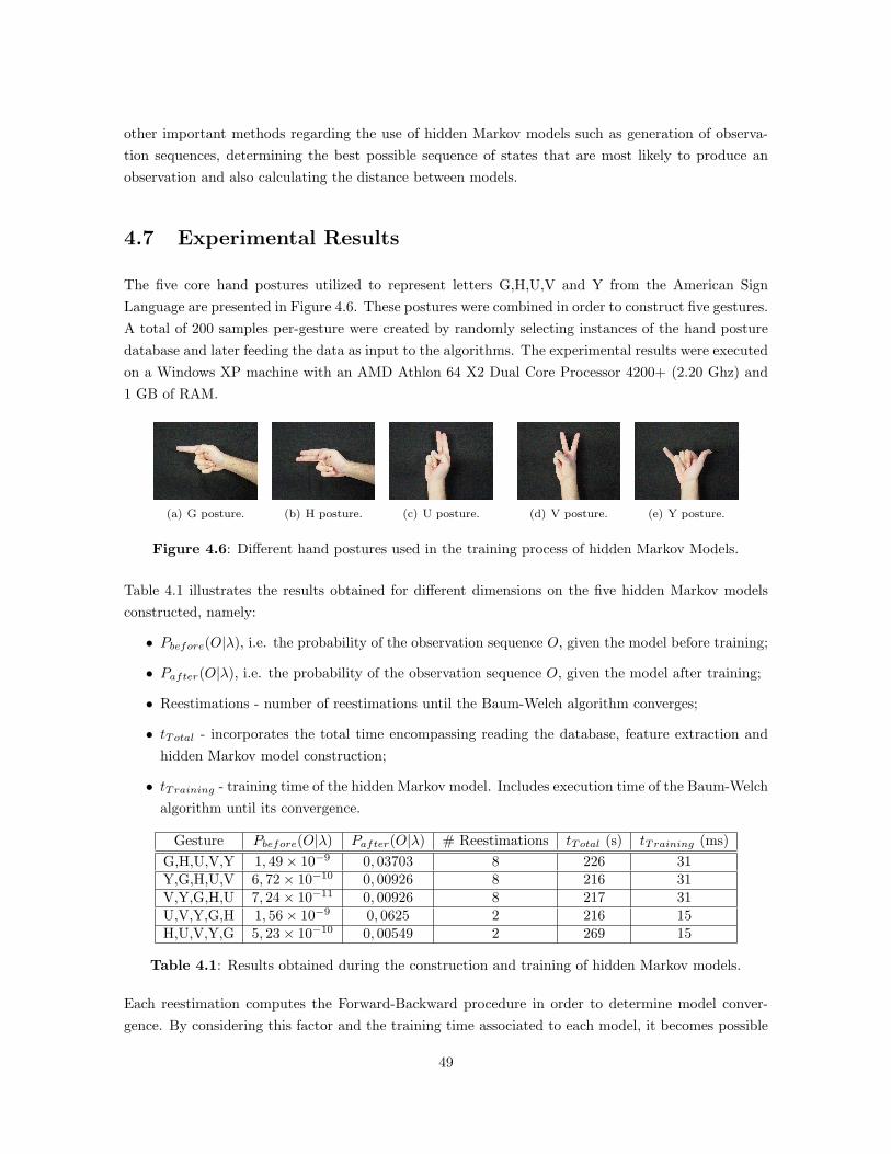
other important methods regarding the use of hidden Markov models such as generation of observa-tion sequences, determining the best possible sequence of states that are most likely to produce anobservation and also calculating the distance between models.

4.7 Experimental Results

The five core hand postures utilized to represent letters G,H,U,V and Y from the American SignLanguage are presented in Figure 4.6. These postures were combined in order to construct five gestures.A total of 200 samples per-gesture were created by randomly selecting instances of the hand posturedatabase and later feeding the data as input to the algorithms. The experimental results were executedon a Windows XP machine with an AMD Athlon 64 X2 Dual Core Processor 4200+ (2.20 Ghz) and1 GB of RAM.

(a) G posture. (b) H posture. (c) U posture. (d) V posture. (e) Y posture.

Figure 4.6: Different hand postures used in the training process of hidden Markov Models.

Table 4.1 illustrates the results obtained for different dimensions on the five hidden Markov modelsconstructed, namely:

• Pbefore(O|λ), i.e. the probability of the observation sequence O, given the model before training;

• Pafter(O|λ), i.e. the probability of the observation sequence O, given the model after training;

• Reestimations - number of reestimations until the Baum-Welch algorithm converges;

• tTotal - incorporates the total time encompassing reading the database, feature extraction andhidden Markov model construction;

• tTraining - training time of the hidden Markov model. Includes execution time of the Baum-Welchalgorithm until its convergence.

Gesture Pbefore(O|λ) Pafter(O|λ) # Reestimations tTotal (s) tTraining (ms)G,H,U,V,Y 1, 49× 10−9 0, 03703 8 226 31Y,G,H,U,V 6, 72× 10−10 0, 00926 8 216 31V,Y,G,H,U 7, 24× 10−11 0, 00926 8 217 31U,V,Y,G,H 1, 56× 10−9 0, 0625 2 216 15H,U,V,Y,G 5, 23× 10−10 0, 00549 2 269 15

Table 4.1: Results obtained during the construction and training of hidden Markov models.

Each reestimation computes the Forward-Backward procedure in order to determine model conver-gence. By considering this factor and the training time associated to each model, it becomes possible

49

to obtain an average execution time regarding the calculation of P (O|λ),

tP (O|λ) =318 × 3 + 15

2 × 25

= 5, 325 ms (4.27)

The results obtained, regarding time-wise execution, seem to be in accordance with [Rabiner, 1989],with the bulk of the execution time being spent during the training process and with short times forthe Forward-Backward procedure.

Another important point to mention regards the calculation of P (O|λ) with observation sequences notbelonging to the hidden Markov models against which they were tested. In these cases the value ofP (O|λ) was always zero. Considering that the model with the highest probability P (O|λ) wins, thepreviously mentioned factor could act as an optimization factor.

4.8 Summary

In this chapter, an introduction to hidden Markov models and respective applicability for recognizingmodeling sequences was presented. The main attributes of hidden Markov models, as well as problemsand respective solutions, were presented. The analysis of the experimental results seems to provideconsistency to the thesis that hidden Markov models are well suited for fast probability computationof observation sequences.

50

Chapter 5

System Implementation

5.1 Introduction

In embedded-systems design it is essential to weigh the functional requirements of a given applicationagainst constraints such as performance, cost, size, power dissipation, energy consumption and weight.It is also necessary to consider whether a functional component will be implemented in hardware oras software. [Sangiovanni-Vincentelly and Martin, 2001] draws attention to the fact that increasinglycomplex functional requirements alongside ever-changing system specifications has resulted in a cleartrend towards flexible implementations. Also important to consider are the mounting levels of com-putational power associated with decreasing trends in size and cost that have allowed designers tomove increasing amounts of functionality to software. These factors combined with the expensiveand time-consuming nature of hardware-manufacturing cycles have favored the popularity of softwarebased implementations.

Considering the core component involved in the gesture recognition system developed in this work,i.e. the smartphone, and it being a programmable device, it is natural that system implementationwill assume a clear software based dimension. The remaining sections of this chapter are organized toreflect the components used and also the development cycle approach towards system implementation,namely:

• Section 5.2 - presents the main features regarding hardware, software and Java Virtual Machine(JVM) technology, of the smartphones used during system development;

• Section 5.3 - presents a detailed analysis of the system architecture encompassing:

– Section 5.3.1 - Development cycle utilized, respective stages, functional cores defined duringsystem development as well as a set of rules derived to facilitate application migrationbetween platforms;

– Section 5.3.2 - System deployment diagram, core execution nodes and description of respec-tive components executing in each of those.

51

5.2 Smartphone Component

With a predicted number of over 2 billion global mobile subscribers for 2008 [Neuvo, 2004], the cellularphone has become one of most pervasive pocket-carried devices. Old models of cellular phones pos-sessed very limited processing power and mainly focused on voice and data transfer between cellularnetworks and respective users. The smartphone distinguishes itself from its predecessors by combiningsignificantly more computing power, memory, short-range wireless communication (e.g. Bluetooth)and a diverse set of input-output components such as digital cameras, accelerometers and MP3 players[Iftode et al., 2004].

Perhaps one of the most important characteristics of a smartphone is that it is a programmable device.Traditionally, each smartphone vendor has provided a native programming languages in accordancewith a built-in operating system, such as Symbian C++ (see [Nokia, 2008]). Recent efforts towardsstandardization and multi-platform support have focused on empowering the Java language. Accordingto [Neuvo, 2004], Java represents the desired platform for enabling the deployment of mobile services. Aspecific version of the Java language, the Java Platform Micro Edition (J2ME) (for further informationsee [Sun, 2008a]), has been developed to meet the inherent resource constraints of embedded systems.J2ME provides a flexible environment for applications targeting smartphones and other embeddeddevices. Applications based on J2ME are portable across many devices. For this reason, Java representsthe primary platform for deploying third-party applications targeting a wide variety of devices.

During the realization of this master thesis two smartphones were used, namely Nokia’s N80 and N95models (presented in Figure 5.1(a) and Figure 5.1(b)), which feature respectively 3 and 5 megapixelscameras.

Although Nokia does not publicly reveal the details about the processors incorporated into their hand-sets it is still possible to obtain that information. The Federal Communications Commission is anindependent United States government agency charged with regulating interstate and internationalcommunications by radio, television, wire, satellite and cable [FCC, 2008]. As part of its responsi-bilities the FCC’s Wireless Telecommunications Bureau conducts conformity regulation tests on allcellular phones commercially available in the United States. The N80 and N95 are both availablein United States territory and as such were subjected to FCC tests which were made publicly avail-able (see [FCC, 2006] and [FCC, 2005]). As such, it is possible to know which processors equip eachhandset.

Nokia’s N95 model boasts a Texas Instrument’s OMAP2420 processor whilst the N80 model featuresan OMAP1710 (for further details check Figure B.2 and Figure B.1 respectively). The OMAP2420 andOMAP1710 processors are single-chip solutions that support all cellular standards. Texas InstrumentsOMAP2420 features an ARM1136, presented in Figure B.4, processor core clocked at 330 Mhz whilstOMAP1710 features an ARM926TEJ, presented in Figure B.3, clocked at 220 Mhz (see [TI, 2008b]and [TI, 2008a]).

Figure B.2 and Figure B.1 illustrate that both architectures are already multi-core computing platformswith independent cores for application processing, digital signal processing, and also 2D/3D graphics

52

(a) Nokia’s N95. (b) Nokia’s N80.

Figure 5.1: The two smartphones used for system development.

acceleration [TI, 2008b] [TI, 2008a]. These factors enable the smartphones used to have the computingpower necessary to execute a wide-range of applications and the work done in this master thesis willprovide examples corroborating this.

Both OMAP processors feature Jazelle technology which is a combined hardware and software solutionfrom ARM. According to [ARM, 2008a] ARM’s Jazelle technology software is a full feature multi-tasking JVM, optimized to take advantage of Jazelle technology architecture extensions available inmany ARM processor cores. ARM Jazelle software includes technology to enable Jazelle hardware inany existing JVM and Java platform. It also includes a full featured multi-tasking Virtual Machine(MVM) that is integrated into many Java platforms. By utilizing the underlying Jazelle technologyarchitecture extensions, the ARM MVM software solution enables higher performance, faster start-upand application switching with a very low memory and power budget.

Figure 5.2: Jazelle technology core functional blocks (source:[ARM, 2008a]).

53

5.3 System Architecture

5.3.1 Development Cycle

Many embedded systems have substantially different design constraints than desktop computing ap-plications. The combination of factors such as cost sensitivity, long life cycle, real-time and reliabilityrequirements impose a different mindset that makes it difficult to adopt traditional computer designmethodologies and tools to embedded systems. Thus, no single characterization applies to the diversespectrum of embedded systems [Koopman, 1996].

In the case of the work developed for this master thesis, the development cycle used is illustratedin Figure 5.3 and described next. Typical design methodologies start with a requirement capturephase characterizing the functional and non-functional requirements of an application. This phase isusually followed by an application architecture defining the execution flow and requirements complianceresponsibility associated to each functional block. The combination of requirements capture associatedto the definition of an application architecture, expressed as Stage 1 in Figure 5.3, resulted in thefollowing functional cores for this gesture recognition system:

1. Skin Detection Phase

In charge of image acquisition and respective data processing in order to distinguish betweenforeground and background and thus enabling the determination of image pixels that could beskin-labeled. The core details and issues embodying this phase were characterized in Chapter 2.This initial stage also provides the desired input data to the Posture Classification Phase;

2. Posture Classification Phase

In charge of posture database creation, processing and manipulation and whose main responsi-bility would be to classify a given input image provided by the Skin Detection Phase against atrained database. The core details and issues embodying this phase were characterized in Chap-ter 3. This intermediate stage also provides the desired input data to the Gesture ClassificationPhase;

3. Gesture Classification Phase

In charge of gesture database creation, processing and manipulation, namely the acquisition andtraining process of the hidden Markov models representing gestures. Besides these responsibili-ties, the Gesture Classification Phase is also liable for determining to which gesture a given setof postures belongs to. The core details and issues embodying this phase were characterized inChapter 4.

4. Action Performer

In charge of making sure that an action sequence associated to a gesture is transmitted to theLEGO NXT component. The core details and issues embodying this phase are characterized inAppendix A.

54

Once the core functional blocks of the application architecture were defined work proceeded as fol-lows:

• For each functional core a proof of concept was performed using Java Standard Edition (J2SE)represented as Stage 2 of Figure 5.3. A standard computer application, presented in FigureC.1, was developed featuring all functional cores. The application served as a simulator allowingfor parameters specification and result observation. If the proof of concept did not meet therequirements defined for that functional block then further refinement would be performed on it.

Due to the different operational audience of J2ME, which targets resource constrained devices,not every class of the plentiful J2SE API exists in J2ME. This is particularly true regardingdata structure availability and also features such as built-in iteration mechanisms. With theselimitations in mind and in order to ensure successful migration between platorms, a set of strategicrules was divised, namely:

– Rule 1 - Only use API methods available in both J2SE and J2ME;

– Rule 2 - Substitute J2SE native data structures by a combination of purpose-built datastructures, Vector and Hashtable classes;

– Rule 3 - Guarantee that all purpose-built data structures override the methods of theEnumeration interface;

– Rule 4 - Substitute all J2SE standard iteration mechanisms with calls to the Enumerationinterface;

– Rule 5 - Exercise great care when allocating objects and take all possible steps to avoidholding references to objects longer than necessary, in order to allow the garbage collectorto reclaim heap space as quickly as possible.

• Each time a functional core was deemed as having an adequate behavior and performance itwas migrated to a J2ME Mobile Information Device Profile (MIDP) application, also known asMIDlet, represented as Stage 3 of Figure 5.3. The migration process required a careful applicationadaptation effort as there would be portions of code, such as database creation and experimentaltests, that were not necessary for MIDlet execution. Once the migration process was concludedthe MIDlet was tested on Sun’s Java Wireless Toolkit (WTK) 2.5.2 emulator in order to checkfor proper compliance within emulator specifications. Besides enabling specification of memoryrestrictions, Sun’s WTK also provides a series of tools in order to profile memory usage and CPUperformance, thus enabling bottleneck detection. If the tests performed on the MIDlet revealedthe existence of performance hampering bottlenecks, optimization techniques would be appliedto those portions of the code and further MIDlet reassessment would be made;

• Once the MIDlet achieved the desired behavior, it would be loaded into the smartphones andtested, expressed as Stage 4 of Figure 5.3. At this stage of development, the main test concernsregarded performance issues such as algorithm execution, memory issues such as ensuring thatthe application did not run out of memory and also fine tuning parameters such as cameraresolution in order to obtain the best balance between speed and quality;

55

• If at any given time it was concluded that an implementation strategy was not suited due toperformance issues, further refinement would be made in the previous stages.

Figure 5.3: Development cycle characterization.

5.3.2 Deployment Model

Given the restrictions associated with embedded systems and the development cycle employed, it isnatural that system architecture will vary considerably until the final stages of system development.Final system architecture for the gesture recognition system presented in this work is illustrated inFigure 5.4 which depicts an UML 2 deployment diagram. An UML 2 deployment diagram describes astatic view of the run-time configuration of processing nodes and the components executing on thosenodes. In other words, deployment diagrams show the hardware of the system, the software that isinstalled on that hardware, and the middleware used to connect the disparate nodes to one another[Fowler, 2003]. For information regarding the domain model of this work please refer to AppendixD.

56

As it is possible to check from Figure 5.4, three core execution nodes exist that provide an executionenvironment for a given set of components. Those core nodes alongside a description of the componentscontained in them are presented next:

• Lego NXT

– NXT Middleware - Server side

Responsible for managing bluetooth connections, disconnections, NXT configuration issuesand command execution.

• Desktop Workstation

– Posture Database Training

Responsible for posture database creation in the form of an Extensible Markup Language(XML) file containing the features characterizing a given set of hand postures image files;

– Gesture Database Training

Responsible for gesture database creation in the form of an XML file containing the paths tothe hidden Markov models depicting each gesture. Other tasks featured in this componentinclude generation of a sample database containing a given set of hand postures depictinga gesture and also Baum-Welch algorithm execution in order to fine-tune hidden Markovmodels.

• Smartphone

– Posture Database

Enabling XML file interpretation, provided by the Posture Database Training compo-nent, in order to obtain the main features of the hand postures used in database trainingand thus allowing for the creation of a hand posture database.

– Gesture Database

Enabling XML file interpretation, provided by the Gesture Database Training compo-nent, in order to obtain the hidden Markov models, and associated actions, depicting eachgesture used in database training and thus allowing for the creation of a gesture database.

– Video Camera

MMAPI component enabling control over video display and image acquisition providing theinitial input to the gesture recognition system;

– Posture Recognition

Allowing for posture classification of a given input image, provided by the Video Camera

component. Due to the large and complex array of functions under the responsibility of thePosture Recognition component and in order to maintain a flexible and modular systemarchitecture the following sub-components were created:

57

∗ Feature Extractor

Responsible for determining the features describing an input image. Again, in order tomaintain modularity the following sub-components were created:

· Skin Detection

Responsible for determining which pixels of the input image can be labeled as skin;

· Reduce Filter

Responsible for scaling an image to a given resolution and removal of salt-and-pepper noise;

· Connected Components Filter

Responsible for determining the largest area of skin pixels present on the filteredimage;

· Image Centralization

Responsible for centering the pixels of a given posture;

· Skin Point

Responsible for computing the features of the simple pattern recognition method.

∗ Classifier

Allowing for encapsulation of the classifier algorithm used,

· K Nearest Neighbors

In charge of determining the k nearest neighbors to the features provided by theFeature Extraction component in order to classify to which posture class themajority of them belongs to.

– Gesture Recognition

In charge of determining the most likely gesture representing a given set of postures, pro-vided by the Posture Recognition component. In reality, this component calculates theprobability of an observation sequence being generated with the hidden Markov modelspresent in the gesture database;

– Action Performer

Responsible for ensuring that a given set of actions belonging to a gesture are executed;

– NXT Middleware Client

Responsible for managing bluetooth connections and disconnections with the Lego NXT

Middleware Server component as well as conveying command requests.

58

Figure 5.4: System Architecture.

59

5.4 Summary

In this chapter we introduced the technology used and core components of this gesture recognitionsystem. An analysis focusing on technological features of Nokia’s smartphone models was performed.We included a detailed analysis of the development cycle, and respective issues, utilized during systemdevelopment. The system’s core execution nodes and description of respective components executingin each of those were then analyzed.

60

Chapter 6

Experimental Results

6.1 Introduction

All of the experimental results presented on the previous chapters focused entirely on individual systemcomponents. This chapter describes the experiments that were performed in order to evaluate systemperformance, as well as discuss the impact of the results obtained.

In the case of this work, besides the evident performance issue regarding how many correct results wereachieved by this gesture recognition system it is also crucial to consider its core execution platform,i.e., smartphones. Note that one of the main objectives of this work is to assess current smartphoneperformance, considering not only computational power but also camera wise.

In order to consider the impact of these factors, amongst other issues, this chapter is organized asfollows:

• Section 6.2 - Describes the main tests performed on Nokia’s N80 and N95 smartphone models.The tests performed focused on execution times for:

– Section 6.2.1 - Image acquisition times through the built-in cameras;

– Section 6.2.2 - Operation times for a specific set of low-level arithmetic instructions;

– Section 6.2.3 - System execution time focusing on hand posture classification;

• Section 6.3 - Describes the results of profiling the final gesture recognition system in order toassess execution times and bottleneck detection;

• Section 6.4 - Presents the experimental setup and results obtained for this gesture recognitionsystem.

61

6.2 Smartphone Performance

J2ME grants access to a phone’s camera through the optional library Mobile Media API (MMAPI)(see [Sun, 2008b]) which provides audio, video and other multimedia support to resource-constraineddevices. MMAPI enables Java developers to gain access to native multimedia services available on agiven device thus enabling the development of multimedia applications targeting smartphones fromdifferent manufacturers.

Applications such as this gesture recognition system whose main focus is on pattern recognitionrely heavily on image acquisition and processing. If an image processing application is to be built,the smartphone must be able to execute computationally expensive algorithms as well as acquireimages at a significant acquisition rate. Factors like image processing and camera access perfor-mance in J2ME should be properly analyzed has they carry possible implications for the application[Tierno and Campo, 2005].

6.2.1 Camera performance

MMAPI enables video snapshot acquisition, which can be used for creation of immutable instancesof the javax.microedition.lcdui.Image class. MMAPI also allows one to obtain the RGB pixel valuesfrom an image in order to proceed with data processing. The combination of these three proce-dures corresponds to the steps required in order to execute some useful computation over a givenimage and as such the combined total time can be interpreted as representing the acquisition time[Tierno and Campo, 2005]. Figure 6.1 illustrates the average acquisition times obtained for Nokia’sN80 and N95 models with MMAPI. For each resolution mode ten image processing iterations wereperformed (contemplating the three procedures mentioned above). A total of 120 tests were per-formed.

It should be noted that the N80 and N95 smartphones boast different cameras, each with its uniqueset of characteristics, such as auto-focus and red-eye reduction, that could not be directly manip-ulated by the API. In order to provide accurate results regarding camera performance it wouldhave been important to control such features. Also noteworthy is the fact that theoretically the 3mega pixels camera should provide for resolutions up to 2048 × 1536 whilst the 5 mega pixels modelshould be capable of achieving up to 2592× 1944. Yet the maximum resolution that we were able toachieve was 800× 600, with higher resolutions not being available and requests for those generating ajavax.microedition.media.MediaException exception.

As it is possible to see, using J2ME both models present relatively high acquisition times, evenfor such low resolutions as 160 × 120, making it impossible to meet real-time requirements. Alsonoteworthy is the fact that both models present an acquisition time drop for the 640 × 480 reso-lution which seems to provide consistency to the fact that this resolution represents the standardoperating mode for both cameras, with the remaining resolutions being obtained using re-scales[Tierno and Campo, 2005].

62

It is also important to draw attention to the fact that from a smoothness operational perspective,the N95 MMAPI implementation, regarding camera functionality, operated in a consistent mannerthroughout system development. The same could not be said for the N80 MMAPI implementationwhich systematically and randomly raised exceptions.

Figure 6.1: Image acquisition times regarding image resolution.

6.2.2 Low-level operations performance

Regarding J2ME processing performance in the N80 and N95, we measured the processor’s executiontime for basic low-level operations to determine the overall speed and to identify the fastest and slowestoperations. In order to obtain time measurements we used Java’s System.currentTimeMillis() methodwhich allows for a precision in milliseconds. Each operation was executed in a loop of 10.000.000iterations and the total execution time of loop was measured. In order to counter the effects of loopspecific instructions, such as increments and comparisons, the total execution time of an empty loopwith the same number of iterations was measured. The duration of each operation corresponds to anaverage between the time of first loop minus the empty loop, over the number of iterations. An averagemeasure was chosen because the application was executed concurrently with other processes runningon the smartphone’s operating system. This procedure was then applied to measure how long it tookto:

• access an array;

• increment an integer variable;

• add two integer variables;

• use bit shift operators to multiply and divide integers by a power of 2;

• use the multiplication operator to multiply two integer variables;

• use the division operator to divide by two integer variables;

63

• compare two variables (equal, less or equal, less).

The results presented in Figure 6.2 reveal the execution times for each operation. In both smartphonesmodels, division is the slowest operation followed respectively by array extractions, compare operatorsand finally other arithmetic operations. Although the N80 and N95 feature different base ARMprocessors and one expected to see better performance from the latter, it was still surprising to checkthat regarding the less or equal operation, the N95 was more than three times slower than the N80.Regarding the remaining operations it is possible to check a clear performance superiority of theN95.

Figure 6.2: Operation times regarding low-level arithmetic operations.

6.2.3 System execution time performance

In order to assess the impact of each smartphone computing power in the final gesture recognitionsystem, a total of 50 hand posture classifications per smartphone were conducted. The hand postureclassification was chosen as it conveys information regarding the execution times associated with theposture labeling of each input image in an acquisition time-wise independent fashion. This situationcontrasts with the system’s attempts at determining to which gesture a given set of postures belongs.In order to do so it is necessary to take into account the total time between acquiring an initial imageand calculating the most probable gesture.

The final system, as presented in Chapter 5, was deployed onto both smartphone models. Table 6.1illustrates the average execution times per hand posture considering a resolution of 320 × 240 pixels,as well as respective maximum frames per second (FPS) allowed for those values, obtained for Nokia’sN80 and N95 models.

Nokia N80 Nokia N95Average Execution Time (ms) 4935 1036

Maximum FPS (s) 0.202 0.965

Table 6.1: Average execution times per hand posture and maximum FPS.

64

The results obtained demonstrate a clear superiority, regarding execution times, for the N95 smart-phone. In average, Nokia’s N80 model was over four times slower when comparing with the N95results. The N95 smartphone results allow for an input frequency of approximately a hand postureper second.

If one considers a real-world application of a gesture recognition system for smartphones this value,of a hand posture per second, seems reasonable and enables a real-time use. On the other hand, theN80 achieves a maximum value of 0.202 frames per second, which is considerably lower and would notallow for a desirable user experience.

The combination of MMAPI stability alongside better performance results were deciding factors thatcontributed to our final decision of using Nokia’s N95 model as the smartphone component for finalsystem testing.

6.3 Profiling

In software engineering, profiling represents the investigation of a program’s behavior using informationcollected during program execution [Gupta, 2005]. The most common goal of profiling an applicationconsists in determining which parts of a program are more likely to provide substantial gains in terms ofspeed or memory footprint by enabling bottlenecks detection. According to [Gupta, 2005] performancebottlenecks represent regions of an application’s code that play a key role in the total execution timeof the program. Once a performance bottleneck has been identified it becomes possible to conduct animprovement study that could potentially have a significant impact on an application’s performance.Sun’s WTK, which was used during system development, incorporates a profiler, enabling behaviormeasurement during program execution using emulators, focusing on the frequency and duration offunction calls. It outputs a statistical summary of the events observed. It should be noted that differentmeasurements along a timeline will result in different profiling data.

Figure 6.3 illustrates a summary of the the profiling results obtained for the application’s initializationand execution phase after one gesture and after ten gestures were presented to the system, respectively.As it is possible to check from Figure 6.3(a), after only one gesture has been introduced most of exe-cution time, respectively 83.58%, relies on the initialization process which includes database retrievaland appropriate data structure creation. Of the total execution time, only 12, 45% was dedicated tocomputing the most probable gesture, i.e. the execution phase of the application. When ten gestureswere presented as input to the system, see Figure 6.3(b), the execution phase increased to 91.39% oftotal execution time, whilst the initialization dropped to 6.54%.

Within the initialization phase, it is possible to distinguish between two core sub-components, namelythe Posture Database and the Gesture Database, which were described in Chapter 5. As it is possibleto see from Figure 6.4, both processes present nearly identical time distributions for one and tengestures. This was expected as the initialization phase is only executed once (when the applicationstarts) whilst the execution phase is run throughout the application execution.

65

(a) Initialization vs Execution (1 Gesture). (b) Initialization vs Execution (10 Gestures).

Figure 6.3: Application profiling of the total execution time distribution for Initialization andExecution phases.

(a) Initialization (1 Gesture). (b) Initialization (10 Gestures).

Figure 6.4: Profiling of the total execution time distribution for Initialization phase.

By delving deeper into the execution phase, as illustrated by Figure 6.5, it becomes possible to dis-tinguish a number of sub-components, which were described in Chapter 5. As was expected intensecomputer vision algorithms claim the greatest share of the execution time distribution, namely the SkinDetection and Connected Components Filter components. Both these components start by represent-ing over 75.34% and end up with 91.34%, as illustrated by Figure 6.5(a) and Figure 6.5(b), respectively.This situation was to be expected as both components represent pixel intensive operations that besidesanalyzing every pixel of an input image also conduct a neighborhood survey over filtered images. Thehand posture recognition method applied during system profiling was the simple pattern recognitionmethod described in Chapter 3, which, due to a low execution time, is not represented in the executionpie charts.

Clearly, in order to tackle the system’s execution time it becomes necessary to address the performanceissues surrounding these two components and to consider possible optimization techniques, such asloop optimization techniques, namely loop unrolling, loop fusion, loop fission and loop splitting, asconversion to lower cost arithmetic operations.

66

(a) Execution (1 Gesture). (b) Execution (10 Gestures).

Figure 6.5: Profiling of the total execution time distribution for Execution phase.

6.4 Final system performance

6.4.1 Experimental Setup

In order to test this gesture recognition system, we proceeded with the experimental setup demon-strated by Figure 6.6, which illustrates the following factors:

• Figure 6.6(a) - Due to a lack of scaling mechanisms within this gesture recognition system, specialcare was taken with the distance between smartphone and hand gestures. A simple measuringtape was employed in order to ensure proper distance compliance between experimental setupand the images employed for training set creation regarding hand postures;

• Figure 6.6(b) - Illustrates the capture view associated with the N95’s built-in camera. The imagedepicts an office room under natural lighting conditions and with an abundance of backgroundobjects. These factors, alongside not being a simple black background, allow the image to beclassified as a complex background;

• Figure 6.6(c) - The system was deployed onto Nokia’s N95 smartphone and gestures were pre-sented to the system according to a previous established distance. During the duration of thetests the smartphone remained at a fixed position. Each time a posture was processed an audiosignal notified the user that a new posture could be introduced to the system.

The gestures classes, presented in Figures 6.7, 6.8 and 6.9, used for system testing, were labeledrespectively as Gesture 1, Gesture 2 and Gesture 3. For each gesture class defined, 30 gestures instancesper class were presented to the system. Given the tree core gesture classes defined and the 30 instancesper class, a total of 90 gestures were employed during system testing.

Each gesture was also mapped into a set of NXT actions to be carried out by the ActionPerformer andNXT components described in Chapter 5. Table 6.2 presents the mapping performed between eachgesture and a corresponding set of actions that are directly carried out by the NXT’s middleware (forfurther details consult Appendix A).

67

(a) Experimental Setup. (b) Capture View. (c) Test Example.

Figure 6.6: Experimental Setup.

(a) InitialPosture.

(b) Posture2.

(c) Posture3.

(d) Posture4.

(e) End Pos-ture.

Figure 6.7: Gesture 1.

(a) InitialPosture.

(b) Posture2.

(c) Posture3.

(d) Posture4.

(e) End Pos-ture.

Figure 6.8: Gesture 2.

(a) InitialPosture.

(b) Posture2.

(c) Posture3.

(d) Posture4.

(e) End Pos-ture.

Figure 6.9: Gesture 3.

Gesture Class ActionPerformer action Middleware API calls1 Front travel(30)

Back travel(-30)Left rotate(180)

Right rotate(-180)2 Front travel(30)3 Back travel(-30)

Table 6.2: Mapping between gestures and NXT actions.

68

6.4.2 Results

Figure 6.10 illustrates the precisions obtained for the three gestures defined. Next we discuss theseresults:

• Gesture class three has a slight advantage over the remaining classes. This was expected asthe HMM model depicting this gesture presents a higher observation probability, 25%, overthe remaining HMMs, 6.25% and 12.5% for Gesture 1 and Gesture 2, respectively. In thiscase, higher probability translates directly into a more likely class three classification, despite ofpossible posture misclassifications. Accordingly, most gesture misclassifications verified were dueto this higher probability, with the system erroneously classifying gestures as belonging to classthree.

• The misclassified gestures were due to errors introduced by significant posture variations and skindetection errors that had a direct impact on hand posture classification. Every time the systemcorrectly classified individual hand postures the correct gesture would be returned. Otherwisethe system would attempt to retrieve the most likely gesture, in accordance with the forwardand backward algorithms presented in Chapter 4.

• Correct gesture classifications strongly depended on correct individual posture classification. Inthis case, the number of correct posture hits is in accordance with the results presented regardingposture classification in Chapter 3.

Figure 6.10: Final system precision results.

Considering the precision obtained for the three gesture classes it becomes possible to obtain an averageprecision value of,

Precision =

N∑i=1

Precision(Gesturei)

N=

83% + 80% + 87%3

= 83.3%

69

This average precision value behaves moderately when compared with other gesture recognition sys-tems, specially if one consider the far simpler techniques employed in this work, namely:

• [Jota et al., 2006] - Obtains average recognitions rates around 93% using two separate techniquesin conjunction with simple black backgrounds. The first technique recognizes bare-hands usingits outer contours. The second approach is based on color marks present on each fingertip thatallow for hand tracking and posture recognition;

• [Liang and Ouhyoung, 1998] - A large vocabulary sign language interpreter using HMMs wasdeveloped using a DataGlove to extract a set of features such as posture, position, orientationand motion. The average recognition rate sustained by the experimental results is 80.4%;

• [Triesch and von der Malsburg, 2002] - A system for classification of hand postures against com-plex backgrounds was developed employing elastic graph matching. The system obtains anaverage 86.2% correct classification.

6.5 Summary

In this chapter, a discussion of the main experimental results obtained by the gesture recognition systemdeveloped in this work were presented. The experimental results focused on two core components, thesystem itself and also the smartphones where it would be executed. Two smartphone models, Nokia’sN80 and N95 models, were analyzed regarding their built-in camera, low-level arithmetic operationsand system execution performance. The experimental results favored the use of Nokia’s N95 model.An analysis of the system performance was presented. The experimental results show an averagesystem precision of 83.3%.

70

Chapter 7

Conclusions

The need to improve communication between humans and computers has been crucial in defining newcommunication models, and new ways of interacting with machines. Sign language is a frequently usedtool when the use of voice is impossible, or when the action of writing and typing is difficult, but thepossibility of vision exists. Gestures are thus suited to convey information for which other modalitiesare not efficient.

The recent proliferation of latest generation smartphones featuring advanced capabilities has allowedthe development of a compact and mobile system with many advanced features. A vision basedapproach to gesture recognition was performed by using the built-in cameras included in most oftoday’s smartphones. By developing an approach considering the real-time requirements associated togesture recognition and respective constraints associated to embedded systems, such as smartphones, itwas possible to study the implications of such an interaction process. Since sign language is gesticulatedfluently and interactively like other spoken languages, a gesture recognizer must be able to recognizecontinuous sign vocabularies and attempt do it in an efficient manner.

This thesis presents a gesture recognition system based on J2ME which has been developed to meetthe inherent resource constraints of smartphones and other embedded devices. Access to the built-incameras was provided by MMAPI which enabled control over video display and image acquisitionproviding the initial input to the gesture recognition system. During the realization of this masterthesis two smartphones were used, namely Nokia’s N80 and N95 models.

The work started with a study of methods that could potentially help in distinguishing betweenforeground and background objects. Two skin detection methods based on different color spaces,namely RGB and HSI were tested. Based on the experimental results obtained it was possible toconclude that the average precision values for the RGB color space rules outperformed those for theHSI rules, respectively 82.27% and 37.83%. If the default color space provided by the acquisitiondevice is RGB then the computational costs associated to an HSI color space transformation areunjustified. Also noteworthy was the segmentation process high susceptibility to different lightingconditions.

71

System development then proceeded with a reflection considering possible posture recognition mech-anisms. Two methods were developed, a convex hull approach and a simple pattern recognitionapproach. The first method derives models out of hand postures whilst the latter attempts to depicta scene with an appropriate encoding. The former approach obtained an average precision value of47% for a representative background set. Although two variations of the latter were tested, basedon resolution windows of 32 × 24 and 64 × 48, no significant gains were achieved with both versionsscoring an average precision value of 84%. By effectively doubling the resolution window, and thusconveying more information on a per-posture basis, one expected to see an increase in precision, whichwas not verified. The resolution increase also carried significant penalties in memory terms, effectivelydoubling the amount of memory required for each posture. Based on the results obtained, the finalchoice fell on a resolution window of 32 × 24. Since the same set of input images was used to testboth posture recognition mechanisms, and based on the experimental results obtained, it is possibleto state that the simple pattern recognition method’s performance is superior to that of the convexhull.

The feature extraction mechanisms developed for hand posture classification assume a critical dimen-sion when used in conjunction with a classification algorithm. For this work we developed a k-NearestNeighbor classifier and subjected it to a test battery in order to determine an appropriate value fork. The experimental results demonstrate that the highest precision rates were achieved for k = 1,although this is not a desirable situation as it does not take into account feature vector distributionin d-space. It is also important to mention that an inneficient skin detection phase hampers highrecognition rates in the hand posture recognition phase.

Once a posture was classified it became necessary to develop a strategy that would consider a posturealongside others, in order to determine to which gesture the posture set belonged to. We employedhidden Markov models in order to characterize gestures in terms of signal hand postures. The resultsobtained, regarding time-wise execution, demonstrated that the bulk of time consumption occuredduring the training process and with shorter times for the Forward-Backward procedure. The executiontimes for the Forward-Backward procedure, in the order of the tenths of miliseconds, make it possibleto integrate hidden Markov models in applications with real-time requeriments.

Special care was employed during system development in order to ensure compatibility and performanceissues surrounding the core operational platform where the system would execute, i.e. a smartphone.Based on hands-on experience, a set of rules was derived in order to guarantee a smooth transitionbetween J2SE and J2ME.

The work included a series of experimental results focusing on system and smartphone testing. Thetests performed to assess smartphone performance focused on three dimensions, namely: camera,low-level arithmetic operations and system execution performance. Of the tests performed, the mostpenalizing factor was camera performance which exhibited extremely high capture times. Currently,J2ME does not support access to image frames using video capture. The gesture recognition sys-tem developed in this work employed image snapshots, which tests demonstrated, carried significanttime acquisition penalties. The image snapshots high acquisition times hampers its use in real-timeapplications.

72

The remaining tests, which basically attempted to measure each smartphone processing performance,demonstrated that the latest smartphone generation is able to execute computationally expensiveapplications in real-time. Note that the gesture recognition system presented in this thesis makesintensive use of image processing, feature databases, pattern recognition, graph algorithms and alsoprobabilistic models.

7.1 Future Work

Future work on this gesture recognition system includes the possibility of adding the following items,namely:

• Optimize skin detection rules

As previously concluded, the segmentation process is highly susceptible to varying lighting con-ditions. The next generation of smartphones will have built-in light sensors allowing for thedetermination of lighting conditions. These sensors in conjunction with camera specific param-eters, such as ISO sensitivity and lenses characteristics, could potentially work to adjust skindetection rules and consequently improve their precision values.

• Image acquisition employing more than one frame

Currently only one frame is being considered for posture capture. In a real-world approachseveral frames may have to be taken into consideration. This approach would also allow fortrajectories to be taken into consideration in classification algorithms.

• Hidden Markov models implementations

Study the impact of different HMM implementations on the system, with a focus on attemptingto determine the best performing one. Other areas of interest should include training algorithmsprovided and also the migration efforts necessary in converting from J2SE to J2ME.

• Develop and test other classifiers

Currently, only one classifier is being employed in this work, respectively the k-Nearest Neigh-bors. A comprehensive test of other classifiers could potentially reveal one with better overallperformance.

• System testing with other smartphones

Further studies on system execution on different smartphones should be performed not only toassess its behavior but also to determine the feasibility of deploying to a larger spectrum ofmachines.

• Code optimization

With the main bottlenecks detected during system profiling, code optimization techniques couldbe employed potentially yielding significant performance increases.

73

• Scaling and rotation mechanisms

Develop feature extraction techniques employing scaling and rotation mechanisms in order todiminish the system’s lack of tolerance to these factors.

• Feature extraction techniques

Consider other feature extraction techniques that could compensate for significant posture vari-ations introduced by different system end-users.

7.2 Applications

Possible commercial applications for this gesture recognition system include the traditional assistanceto hearing impairment persons. By using a gesture recognition system it becomes possible to conveymeaningful sentences in a more convenient manner than using the traditional short messaging serviceavailable in many mobile network operators.

Gesture recognition in smartphones also opens new possibilities regarding human-computer interac-tions and interfaces. Being able to understand a human being’s movements and actions is of crucialimportance in human-computer interactions. In the future, intended and unintended gestures mightassume a crucial role for a more user satisfying experience. Possible instances of these factors includethe ability to pick up or deny mobile phone calls. Other scenarios include a smartphone being used tomonitor an user in order to pick up possible fatigue signals.

Finally, gesture recognition also assumes a high degree of importance in certain military branchesthat make extensive use of military sign language. In this thesis, the gesture recognition system wasemployed in order to control a Lego NXT robot, equivalent applications could be easily imaginedcontrolling military artifacts.

74

References

[ARM, 2008a] ARM (2008a). Arm jazelle technology. Technical report, ARM Limited.

[ARM, 2008b] ARM (2008b). Arm11 family. http://www.arm.com/products/CPUs/families/

ARM11Family.html, Last visited in July 2008.

[ARM, 2008c] ARM (2008c). Arm926ej-s. http://www.arm.com/products/CPUs/ARM926EJ-S.html,Last visited in July 2008 ,.

[Bahi et al., 1986] Bahi, L. R., Brown, P. F., Souza, P. V. d., and Mercer, R. L. (1986). Maximummutual information estimation of hidden markov model parameters for speech recognition. Proc.Int. Conf. Acoustics, Speech, Signal Processing, 1:49–52.

[Baum, 1972] Baum, L. (1972). An inequality and associated maximization technique in stasticalestimation for probabilistic functions of markov processes. Inequalities, 3:1–8.

[Baum and Egon, 1967] Baum, L. and Egon, J. (1967). An inequality with applications to statisticalestimation for probabilistic functions of a markov process and to a model for ecology. Bull. Amer.Meteorol, 73:360–363.

[Baum et al., 1970] Baum, L., Petrie, T., G., S., and Weiss, N. (1970). A maximization techniqueocurring in the stastical analysis of probabilistic functions of markov chains. Ann. Math. Stat,41:164–171.

[Baum and Sell, 1968] Baum, L. and Sell, G. (1968). Growth functions for transformations on mani-folds. Pac. J.Math., 27:211–227.

[Baum and T., 1966] Baum, L. and T., P. (1966). Statistical inference for probabilistic functions offinite state markov chains. Ann. Math. Stat, 37:1554–1563.

[Bonato et al., 2005] Bonato, V., Sanches, A. K., M.M., F., Cardoso, J. M., Simoes, E., and Marques,E. (2005). A real time gesture recognition system for mobile robots. In review.

[Braffort et al., 1999] Braffort, A., Gherbi, R., Gibet, S., Richardson, J., and Teil, D., editors(1999). Gesture-Based Communication in Human-Computer Interaction, volume 1739, Gif-sur-Yvette, France.

75

[Brand and Mason, 2000] Brand, J. and Mason, J. (2000). A comparative assessment of three ap-proaches to pixel-level human skin-detection. Pattern Recognition, 2000. Proceedings. 15th Interna-tional Conference on, 1:1056–1059 vol.1.

[Bray, 2008] Bray, M. (2008). Middleware: Software technology roadmap. http://www.sei.cmu.edu/str/descriptions/middleware.html, Last visited in June 2008.

[Burge and Karlin, 1997] Burge, C. and Karlin, S. (1997). Prediction of complete gene structures inhuman genomic dna. Journal of Molecular Biology, 268:78–94.

[Canesta, 2008] Canesta (2008). Celluon projection keyboard. http://www.canesta.com/html/

celluon.htm, Last visited in February 2008.

[Carron and Lambert, 1994] Carron, T. and Lambert, P. (13-16 Nov 1994). Color edge detector us-ing jointly hue, saturation and intensity. Image Processing, 1994. Proceedings. ICIP-94., IEEEInternational Conference, 3:977–981 vol.3.

[Coelho, 2008] Coelho, A. (2008). Autonomous mobile robot navigation using smartphone. Master’sthesis, Instituto Superior Tecnico.

[Cormen et al., 2003] Cormen, T., Leiserson, C., Rivest, R., and C., S. (2003). Introduction to Algo-rithms - Second Edition. The MIT Press.

[Cover and Hart, 1967] Cover, T. and Hart, P. (1967). Nearest neighbor pattern classification. Infor-mation Theory, IEEE Transactions on, 13:21–27.

[Cybernet, 2008a] Cybernet (2008a). The gesture storm weather map management system. http:

//www.cybernet.com/products/gesturestorm.html, Last visited in February 2008.

[Cybernet, 2008b] Cybernet (2008b). Navigaze hands free computer control. http://www.cybernet.com/products/navigaze.html, Last visited in February 2008.

[Davis and Shah, 1994] Davis, J. and Shah, M. (Apr 1994). Visual gesture recognition. Vision, Imageand Signal Processing, IEE Proceedings -, 141(2):101–106.

[Dugad and Desai, 1996] Dugad, R. and Desai, U. (1996). A tutorial on hidden markov models. Tech-nical report, Indian Institute of Technology.

[FCC, 2005] FCC (2005). Internal photographs:qfxrm-92. Technical report, Federal CommunicationsCommission.

[FCC, 2006] FCC (2006). Internal photographs:pdnrm-159. Technical report, Federal CommunicationsCommission.

[FCC, 2008] FCC (2008). About the fcc. http://www.fcc.gov/aboutus.html, Last visited in July2008.

[Fowler, 2003] Fowler, M. (2003). UML Distilled: A Brief Guide to the Standard Object ModelingLanguage (3rd Edition). Addison-Wesley Professional.

76

[Gomes and Morales, 2002] Gomes, G. and Morales, E. (2002). Automatic feature construction anda simple rule induction algorithm for skin detection. ICML Workshop on Machine Learning inComputer Vision, .:31–38.

[Gonzalez and Woods, 1992] Gonzalez, R. C. and Woods, R. (1992). Digital Image Processing.Addison-Wesley Company.

[Graham, 1972] Graham, R. (1972). An efficient algorith for determining the convex hull of a finiteplanar set. Information Processing Letters, 1:132–133.

[Gupta, 2005] Gupta, S. C. (2005). Need for speed - eliminating performance bottlenecks: Op-timizing java programs using ibm rational application developer 6.0.1. http://www.ibm.com/

developerworks/rational/library/\05/1004_gupta/, Last visited in August 2008.

[Hartigan, 1975] Hartigan, A. (1975). Clustering Algorithms. Wiley.

[Huning, 1993] Huning, H. (1993). A node splitting algorithm that reduces the number of connectionsin a hamming distance classifying network. International Workshop on Artificial Neural Networks,686:102–107.

[Iftode et al., 2004] Iftode, L., Borcea, C., Ravi, N., Kang, P., and Zhou, P. (2004). Smart phone: anembedded system for universal interactions. Distributed Computing Systems, 2004. FTDCS 2004.Proceedings. 10th IEEE International Workshop on Future Trends of, pages 88–94.

[Jones and Rehg, 2002] Jones, M. J. and Rehg, J. M. (2002). Statistical color models with applicationto skin detection. International Journal of Computer Vision, 46:81–96.

[Jota et al., 2006] Jota, R., Ferreira, A., Cerejo, M., Santos, J., Fonseca, M. J., and Jorge, J. A. (2006).Recognizing hand gestures with cali. EUROGRAPHICS, 1981:1–7.

[King et al., 2005] King, L., Nguyen, H., and Taylor, P. (2005). Hands-free head-movement gesturerecognition using artificial neural networks and the magnified gradient function. Engineering inMedicine and Biology Society, 2005. IEEE-EMBS 2005. 27th Annual International Conference ofthe, pages 2063–2066.

[Koopman, 1996] Koopman, P. (1996). Embedded system design issues (the rest of the story). Com-puter Design: VLSI in Computers and Processors, 1996. ICCD ’96. Proceedings., 1996 IEEE In-ternational Conference on, pages 310–317.

[Kovac et al., 2003] Kovac, J., Peer, P., and Solina, F. (2003). Human skin color clustering for facedetection. EUROCON 2003. Computer as a Tool. The IEEE Region 8, 2:144–148 vol.2.

[Liang and Ouhyoung, 1998] Liang, R.-H. and Ouhyoung, M. (1998). A real-time continuous gesturerecognition system for sign language. Proceedings. Third IEEE International Conference on, 1:558–567.

[Lin and Chen, 1991] Lin, X. and Chen, S. (9-11 Apr 1991). Color image segmentation using modifiedhsi system for road following. Robotics and Automation, 1991. Proceedings., 1991 IEEE InternationalConference on, pages 1998–2003 vol.3.

77

[McDaniel, 2004] McDaniel, T. (2004). Java HMMPak v1.2: User Manual. Center for CognitiveUbiquitous Computing, Arizona State University.

[McDaniel, 2008] McDaniel, T. (2008). Hidden markov models. http://www.public.asu.edu/

~tmcdani/hmm.htm, Last visited in May 2008.

[Mckenna et al., 1998] Mckenna, S., Gong, S., and Raja (1998). Modelling facial colour and identitywith gaussian mixtures. Pattern Recognition 31, 12:1883–1892.

[Morrison and McKenna, 2002] Morrison, H. and McKenna, S. J. (2002). Contact-free recognition ofuser-defined gestures as a means of computer access for the physically disabled. Proc. 1st CambridgeWorkshop on Universal Access and Assistive Technology, pages 99–103.

[Neuvo, 2004] Neuvo, Y. (2004). Cellular phones as embedded systems. Solid-State Circuits Confer-ence, 2004. Digest of Technical Papers. ISSCC. 2004 IEEE International, 1:32–37.

[Nintendo, 2008] Nintendo (2008). What is wii? http://www.nintendo.com/wii/what Last visitedin February 2008.

[Nokia, 2008] Nokia (2008). Symbian c++. http://www.forum.nokia.com/main/resources/

technologies/symbian, Last visited in July 2008.

[Poynton, 1995] Poynton, C. A. (1995). Frequently asked questions about colour.

[Purcell et al., 2003] Purcell, T., Donner, C., Cammarano, M., Jensehn, H., and Hanrahan, P. (2003).Photon mapping on programmable graphics hardware. In Proceedings ACM SIGGRAPH/ Euro-graphics Workshop on Graphics Hardware, pages 41–50.

[Rabiner, 1989] Rabiner, L. R. (1989). A tutorial on hidden markov models and selected applicationsin speech recognition. Proceedings of the IEEE, 77:257–286.

[Russel, 1990] Russel, D. (1990). The Principes of Computer Networking. Cambridge University Press.

[Sangiovanni-Vincentelly and Martin, 2001] Sangiovanni-Vincentelly, A. and Martin, G. (2001).Platform-based design and software design methodology for embedded systems. Design and Test ofComputers, 18:23–33.

[School, 2008] School, A. S. L. (2008). Frequently asked questions. http://www.aslschool.org, Lastvisited in February 2008.

[Shapiro and Stockman, 2001] Shapiro, L. G. and Stockman, G. C. (2001). Computer Vision. PrenticeHall.

[Skarbek and Koschan, 1994] Skarbek, W. and Koschan, A. (1994). Colour image segmentation — asurvey. Technical report, Institute for Technical Informatics, Technical University of Berlin.

[Solurzano et al., 2008] Solurzano, J., Bagnall, B., Stuber, J., and Andrews, P. (2008). lejos: Java forlego mindstorms - icommand technology. http://lejos.sourceforge.net/p_technologies/nxt/icommand/icommand.php, Last visited in June 2008.

[Sun, 2008a] Sun (2008a). Java me at a glance. Technical report, Sun Microsytems.

78

[Sun, 2008b] Sun (2008b). Mobile media api (mmapi); jsr 135. http://java.sun.com/products/

mmapi/, Last visited in July 2008.

[Swenson, 2002] Swenson, R. (2002). A real-time high performance universal colour transformationhardware system. PhD thesis, University of Kent at Canterbury.

[TI, 2008a] TI (2008a). High-performance: Omap1710. http://focus.ti.com/general/docs/wtbu/\wtbuproductcontent.tsp?templateId=6123\\&navigationId=11991\&contentId=4670, Lastvisited in July 2008 ,.

[TI, 2008b] TI (2008b). High-performance: Omap2420. http://focus.ti.com/general/docs/wtbu/\wtbuproductcontent.tsp?templateId=6123\\&navigationId=11990\&contentId=4671, Lastvisited in July 2008.

[Tierno and Campo, 2005] Tierno, J. and Campo, C. (2005). Smart camera phones: Limits and ap-plications. Pervasive Computing, IEEE, 4:84–87.

[Triesch and von der Malsburg, 2002] Triesch, J. and von der Malsburg, C. (2002). Robust classifi-cation of hand postures against complex backgrounds. Automatic Face and Gesture Recognition,1996., Proceedings of the Second International Conference on, pages 170–175.

[Vezhnevets et al., 2003] Vezhnevets, V., Sazonov, V., and Andreeva, A. (2003). A survey on pixel-based skin color detection techniques.

[Wilson and Bobick, 1999] Wilson, A. D. and Bobick, A. F. (1999). Parametric hidden markov modelsfor gesture recognition. IEEE Transactions on Pattern Analysis and Machine Intelligence, 21:884–900.

[Yamaguchi, 1984] Yamaguchi, H. (Nov 1984). Efficient encoding of colored pictures in r, g, b compo-nents. Communications, IEEE Transactions on [legacy, pre - 1988], 32(11):1201–1209.

[Yu et al., 2001] Yu, C., Ooi, B. C., Tan, K.-L., and Jagadish, H. (2001). Indexing the distance: Anefficient method to knn processing. In Proceedings of the 27th VLDB conference.

[Zarit et al., 1999] Zarit, B., Super, B., and Quek, F. (1999). Comparison of five color models inskin pixel classification. Recognition, Analysis, and Tracking of Faces and Gestures in Real-TimeSystems, 1999. Proceedings. International Workshop on, pages 58–63.

[Zhang and Wang, 2000] Zhang, C. and Wang, P. (2000). A new method of color image segmentationbased on intensity and hue clustering. Pattern Recognition, 2000. Proceedings. 15th InternationalConference on, 3:613–616.

[Zheng et al., 2004] Zheng, H., Daoudi, M., and Jedynak, B. (2004). Blocking adult images based onstatistical skin detection. Electronic Letters on Computer Vision and Image Analysis, 4:1–14.

79

80

Appendix A

Lego Mindstorm NXT Component

A.1 NXT Middleware

The main focus of this work consists in developing applications for two embedded systems, namelya smartphone and a LEGO NXT, with the bulk of the processing algorithms being executed on theformer and the latter exhibiting some sort of behavior as result of the computations. In order toprovide the desired outcome, and with both devices boasting wireless Bluetooth communication, amiddleware component providing a communication layer abstraction was developed. This sectionpresents the middleware component sitting between the smartphone client application and the serverprogram running on top of the leJOS’s NXT firmware.

The main objective of the middleware component is to facilitate application development for thesmartphone/NXT-based mobile robot system. The core functionality of the middleware consists inproviding simple abstractions for Bluetooth communication and also access to the mobile robot’ssensors and actuators. The middleware component was developed in the Java programming languageand was built on top of the leJOS firmware. Due to a similar scope of thesis, the information presentedin this section was written and developed in conjunction with a master degree colleague, Andre Coelho.For more information on Andre Coelho’s master thesis check [Coelho, 2008].

A.1.1 Middleware Component Description

By definition, middleware is a specific piece of software that interconnects and integrates softwarecomponents and allows them to exchange data [Bray, 2008]. Our middleware component interconnectsa server software application running on the leJOS’s mobile robot, with a client software applicationrunning on a smartphone.

81

By sitting itself between the mobile client and the mobile robot (see Figure A.1), the middleware takesresponsability in all integration efforts that need to be taken care of when developing applications forthis system. The core functionalities are provided through the middleware’s core API (presented inTable A.1) which enables the following items:

• Abstraction to Bluetooth communication between the smartphone and the NXT Brick - Blue-tooth discovery, connections and the bidirectional channel for data exchange are created in atransparent way;

• Reduce application development time - Since Bluetooth communication issues are abstracted,the application programmer only needs to worry about the specific details of its aplication logic.The development time is reduced as well as the application’s complexity;

• Access to NXT sensors and actuators - Functional requirements of the mobile robot such as theability to do rotation, forward and backward movements, as well as sensor readings are providedthrough the standard API.

Figure A.1: The interaction process between mobile device and mobile robot.

A.1.2 Usage Example

In this section we examplify the middleware usage through a demo application. Figure A.2 representsthe execution flow for a client application running on a smartphone.The code starts by creating aMobileClientNXT, which is the only object to be created, and provides the communication abstractionswith the NXT Brick as well as the NXT control commands. After a reference to the NXT has beenobtained, a synchronous connect command is issued in order to establish the connection between thesmartphone and the NXT. Once the connection has been established a forward command with a givenvelocity is issued, followed by a rotation command for a given angle. The next command tells the

82

Method Descriptionconnect() Method that performs the connection to the NXT mobile robot.

disconnect() Method that ceases the current connection with the NXT mobilerobot.

forward(velocity) Method that transmits to the NXT the order to move forward ata determined velocity of movement in degrees/second.

backward(velocity) Method that transmits to the NXT the order to move backwardat a determined velocity of movement in degrees/second.

rotate(angle) Method that transmits to the NXT the order to rotate to a specificangle

stop() Method that transmits to the NXT the order to stop any move-ment that it is currently performing.

travel(distance) Method that transmits to the NXT the order to move for a spec-ified distance.

getSensors() Method that requests to the NXT the list of available sensors.getSensorValue(sensor) Method that request a sensor measurement to the NXT.

Table A.1: Middleware methods list.

NXT to stop all action and the execution flow is terminated with a disconnection command in orderto notify the NXT that the smartphone no longer intends to maintain communication.

Algorithm MIDDLEWARE EXAMPLE1. MobileClientNXT nxtClient;2. nxtClient = new MobileClientNXT(BluetoothAddress);3. nxtClient.connect();4. nxtClient.forward(velocity);5. nxtClient.rotate(angle);6. nxtClient.stop();7. nxtClient.disconnect();

Figure A.2: Middleware interaction example.

A.1.3 Related Work

Besides leJOX NXJ, the leJOS development team has a Java package project designated by iCommandto control the NXT brick over a Bluetooth connection. The difference from this project to ours, isthat former uses the standard Lego NXT firmware to receive commands from Java code on a computerwhilst the latter uses the leJOS NXT firmware.

The iCommand project was released in 2006 with the objective of allowing people to start programmingthe NXT brick in the Java programming language while the leJOS firmware was still in development.On the leJOS website [Solurzano et al., 2008] the leJOS development team expresses the intention ofin the future developing the iCommand package compatible with the leJOS NXJ firmware.

83

84

Appendix B

ARM R©Technology

Figure B.1: OMAP1710 core functional blocks (source:[TI, 2008a]).

85

Figure B.2: OMAP2420 core functional blocks (source:[TI, 2008b]).

Figure B.3: ARM926EJ-S core functional blocks (source:[ARM, 2008c]).

86

Figure B.4: ARM1136JF-S core functional blocks (source:[ARM, 2008b]).

87

88

Appendix C

Application screenshots

Figure C.1: Two sreenshots of the J2SE simulation application developped to test the functionalcores.

89

(a) The J2ME application devel-opped identifying a posture.

(b) The J2ME application devel-opped identifying a posture.

(c) The J2ME application devel-opped identifying a gesture andcarrying out a set of actions.

Figure C.2: The J2ME application developed.

90

Appendix D

Domain Model

Figure D.1: Higher-level view of the domain model.

91

Figure D.2: Domain Model Posture Recognition.

92

Figure D.3: Domain Model Gesture Recognition.

93

Figure D.4: Domain Model Filters.

94