A Geometric Morphometric Analysis of the Human Ossa Coxae for Sex Determination

BOSTON UNIVERSITY

SCHOOL OF MEDICINE

Thesis

A GEOMETRIC MORPHOMETRIC ANALYSIS OF THE HUMAN OSSA

COXAE FOR SEX DETERMINATION

by

BRIANNE E. CHARLES

B.A., University of Wisconsin-Milwaukee, 2010

Submitted in partial fulfillment of the

requirements for the degree of

Master of Science

2013

© Copyright by

BRIANNE E. CHARLES

2013

Approved by

First Reader

Jonathan D. Bethard, Ph.D.

Instructor of Forensic Anthropology

Second Reader

Donald F. Siwek, Ph.D.

Assistant Professor of Anatomy and Neurobiology

4

ACKNOWLEDGMENTS

I would like to thank the faculty of the Boston University School of Medicine Forensic

Anthropology program as well as my peers in the program for guidance and insight

throughout the research progress. Thank you to Dr. Dawnie Steadman and the University

of Tennessee-Knoxville for granting me access to the W.M. Bass Donated Skeletal

Collection and for the gracious individuals who have offered their remains or the remains

of their loved ones to be used to further the field of forensic anthropology.

I cannot express the gratitude that I have for my parents. They have opened many doors

for me and I am forever in debt for the love and support that they tirelessly provide.

Thanks also go out to my siblings, who have always set the bar high. They were all

tough acts to follow and friendly competition among family is always a good motivator to

be the best that you can be. Lastly, thank you to my cake friend. You made living alone

in Boston a little less lonely.

5

A GEOMETRIC MORPHOMETRIC ANALYSIS OF THE HUMAN OSSA

COXAE FOR SEX DETERMINATION

BRIANNE E. CHARLES

Boston University School of Medicine, 2013

Major Professor: Jonathan D. Bethard, Ph.D., Instructor of Forensic Anthropology

ABSTRACT

This study compares sexual variation of the human skeletal pelvis through

geometric morphometric analyses. Digitization of the skeletal elements provides the

framework for a multi-faceted examination of shape. The sample used in the study

consists of individuals from the Bass Donated Skeletal Collection, located at the

University of Tennessee-Knoxville. Landmarks digitized for the study are derived from

the 36 points implemented in Joan Bytheway and Anne Ross’s geometric morphometric

study of human innominates (2010). The author hypothesizes that morphological

variation between males and females will be visible to varying degrees throughout the

pelvis, with structures to be compared consisting of the ilium, ischium, pubis, obturator

foramen, and acetabulum. Particular attention will be paid to the pelvic canal, as this area

seems to carry the most sex-specific function of the bone. It is hypothesized that

structures directly contributing to the pelvic canal will be more sexually dimorphic than

peripheral structures. Data points plotted throughout the pelvis will allow for comparison

of various regions. Results indicate that the innominate can be divided into modules with

6

relatively low levels of covariation between them. Greatest amounts of sexual

dimorphism are located at the pubis and ischium. The shape of the acetabulum and

obturator foramen display little variation between the two sexes. Areas that have the

potential for sex determination could be investigated more thoroughly in the future and

may be of use in forensic cases in which remains are incomplete.

vii

TABLE OF CONTENTS

Page

Title Page i

Copyright ii

Approval Page iii

Acknowledgments iv

Abstract v

List of Tables viii

List of Figures ix

List of Abbreviations xi

Chapter 1: Introduction 1

Chapter 2: Previous Research 4

Chapter 3: Methods 29

Chapter 4: Results 53

Chapter 5: Discussion 70

Chapter 6: Conclusions 77

Appendix A: Bytheway and Ross (2010) landmarks 79

Appendix B: Angular comparison of PC and PLS vectors 81

Bibliography 101

Curriculum Vitae 108

8

LIST OF TABLES

Page

Table 3.1. Landmarks. 34

Table 4.1. Independent samples test for PC scores. 54

Table 4.2. Independent samples test for PLS scores. 65

Table 4.3. Modularity subsets. 69

Table A.1. Landmarks and descriptions. 79

Table B.1. P-values: PC (all) vs. PLS1-PLS7. 81







9

LIST OF FIGURES

Page

Figure 2.1. The three bones of the innominate. 7

Figure 2.2. Planes of the pelvis. 7

Figure 2.3. Bytheway and Ross (2010) difference vectors. 27

Figure 3.1. Age distribution of sample. 31

Figure 3.2. Landmarks. 36

Figure 3.3. Landmarks 6, 24, 25, 27, 28, and 29. 37

Figure 3.4. Setup for digitization. 39

Figure 3.5. Procrustes superimposition. 43

Figure 3.6. Wireframe of PC1. 45

Figure 3.7. Wireframes of male PC1 and female PC1. 45

Figure 3.8. Superior and inferior blocks for PLS. 49

Figure 4.1. PCA eigenvalues. 54

Figure 4.2. PC1: axes 1vs. 2. 55


Figure 4.4. PC1: axes 2 vs. 3. 56

Figure 4.5. PC1 vs. PC2. 57




10




Figure 4.12. Female PC1: axes 1 vs. 2. 62

Figure 4.13. Male PC1: axes 1 vs. 2. 62

Figure 4.14. Discriminant and cross-validation scores. 63

Figure 4.15. Wireframe of discriminant analysis. 64

Figure 4.16. Total percent squared variance between Block 1 and Block 2 per

PLS axis.

66

Figure 4.17. PLS1: axes 1 vs. 2. 66



Figure 4.20. PLS1: Block 1 vs. Block 2. 68

Figure 4.21. Modules. 69

Figure 5.1. Five modules of the innominate. 73

11

LIST OF ABBREVIATIONS

A-P Anterior-posterior

CS Centroid size

DFA Discriminant function analysis

GPA General Procrustes analysis

MANCOVA Multivariate analysis of covariance

M-L Medial-lateral

PC Principal component

PCA Principal components analysis

PLS Partial least squares

1

Disclaimer: In this thesis, the term “sex” is used to describe a trait in an individual’s

biological identity. The binary terms male and female reflect sex in this paper and should

not be considered synonymous with cultural indicators of gender.

CHAPTER 1: INTRODUCTION

Sex determination is one of the key elements in developing the biological profile

of an unknown individual. Determining sex is important because other estimations such

as age and stature depend on whether the individual is male or female and accurate

assignments of sex can reduce the field of potential individuals for identification matches

in forensic cases. Reliable methods of sex determination are therefore important tools to

a forensic anthropologist. However, skeletons rarely show only “typical” male or female

traits, requiring an analysis that uses as many sexing techniques as can be applied,

including traditional morphological comparisons and metric measurements (Wienker

1984). In addition, forensic or archaeological remains may be fragmentary or

incomplete, further obscuring potential metric or morphological assessments.

Both metric and nonmetric methods for determining sex are common and vary in

degree of accuracy depending upon the element, the level of dimorphism, and even the

population that the method was created from or is being applied to. A brief glance at

Buikstra and Ubelaker’s Standards for Data Collection from Human Skeletal Remains

(1994) or other human osteology manuals such as White and Folkens (2005) or Bass

(2005) can highlight the handful of traits from the skull and pelvis that are most

2

commonly used by osteologists to determine sex. Characteristics of the skull (i.e., nuchal

crest, mastoid process, supraorbital margin, glabella, and mental eminence) are evaluated

on a scale from 1 to 5 and tend to be more robust in males. Populations have shown to

vary in the sectioning point between males and females in such traits (Walker 2008).

On the pelvis, the greater sciatic notch is evaluated on a graded scale similar to

the skull, yet until recently, the popular Phenice traits could only be applied as a

“present” or “absent.” Klales et al. (2012) has taken a revolutionary step by assigning

each of the Phenice traits a graded scale and weighing them by their individual ability to

determine sex (see Previous Research section). The system presented by Klales et al.

acknowledges the degree of morphological variation that is possible within the

innominate even between individuals of the same sex.

The overall goal of this study is to apply geometric morphometrics to a sample of

skeletons from a collection of modern, well-documented individuals in order to quantify

sexual dimorphism in general as well as differences in expression of sexual variation

between specific regions of the pelvis. The ilium, ischium, pubis, obturator foramen, and

acetabulum will be analyzed together as a whole unit and as separate structures. The

author hypothesizes that morphological variation between males and females will be

observable to varying degrees between the highlighted regions. The growth and

remodeling of the ischium and pubis in particular vary between sexes during puberty and

the pelvic canal has the most sex-specific function of the pelvis. It is hypothesized that

structures directly contributing to the pelvic canal will be more sexually dimorphic than

3

peripheral structures. Because females are considered to be under greater constraints,

intra-sex variability will be tested to determine whether this is actually the case.

Questions addressed in this study include:

1. Is there variation in the degree of dimorphism between regions of the pelvis?

2. Do females have less intra-group variation in morphology than males?

3. Does variation in morphology reflect sex-specific functions of the pelvic canal?

4

CHAPTER 2: PREVIOUS RESEARCH

Sexual Dimorphism and Sex Determination

The determination of sex from the human skeleton is important in forensic

anthropology because it narrows down the field of potential identification matches and

makes it easier to estimate other information from unknown individuals such as ancestry

and age. However, the skeleton is not always found in pristine condition. Trauma,

mortuary practices, or other taphonomic conditions may leave the skeleton damaged or

incomplete so sex determination cannot be dependent solely upon the interpretation of

single elements. Metric and morphological methods utilizing a variety of bones are

therefore advantageous when remains are incomplete.

Cranial and Postcranial Sex Determination

There is extensive research in sex determination that utilizes different bones of the

human body including long bones (İşcan and Miller-Shaivitz 1986; Purkait 2005),

clavicle and scapula (Frutos 2002), mandible (Loth and Henneberg 1996; Saini et al.

2011), and others overviewed in Buikstra and Ubelaker (1994) and Bass (2005). In

general, males tend to have larger elements, making metric discrimination possible

(Saunders and Hoppa 1997; Spradley and Jantz 2011). Males may also have more robust

articular surfaces and landmarks, which may distinguish them from bones of females

(Rogers 1999; Rogers et al. 2000; Vance et al.2011).

5

Discriminant function analysis of the cranium was originally proposed by Giles

and Elliot (1963) to differentiate between sexes. Using 21 combinations of nine distinct

cranial measurements, they developed discriminant functions and male-female dividing

points. Walker (2008) similarly developed discriminant functions using combinations of

five visually-assessed cranial traits (nuchal crest, mastoid process, mental eminence,

orbital margin, and glabella/supra-orbital ridge). Both Walker (2008) and Giles and

Elliot (1963) found that discriminant functions for determining sex performed well, but

they also caution the application of sample-specific functions to other populations.

While many studies have focused on various parts of the skull such as the

craniofacial region (González et al. 2011; Bastir et al. 2011; Kimmerle et al. 2008), there

is much debate over the reported accuracy of craniometrics versus postcranial

measurements in sex estimation. One recent study that compared the accuracy of the

cranium to postcranial elements was presented by Spradley and Jantz (2011). They

generated univariate and multivariate models to determine whether metric measurements

of the cranium, mandible, or postcranium were most effective for sex estimation in

modern American Black and White populations. The authors found significant

differences in both sex and ancestry and confirmed that multivariate analysis of the

postcranial skeleton is better for sex classification than a multivariate analysis of the

cranium.

6

Sexual Dimorphism of the Pelvis

Arguably, the most effective element for sex differentiation is the pelvic bone.

The pelvis, os coxa, or innominate is composed of three separate bones per side. Each

innominate consists of an ilium, ischium, and pubis bone and articulates with the other

innominate at the pubic symphysis (Figure 2.1). Each innominate also articulates with

the sacrum to complete the overall pelvic structure. Throughout this study, the terms os

coxa (pl. ossa coxae) and innominate are used interchangeably and refer to a single

element (mature and one side) unless otherwise specified. The articulated innominates

together as a unit will be referred to as the pelvis to avoid confusion.

Structure and Function of the Pelvis

There are a few terms that are used to describe the different functional regions of

the pelvis. First, a distinction can be made between the false pelvis and the true pelvis.

The false pelvis is superior to the true pelvis and the two regions are delimited by the

pelvic brim (Figure 2.2). The pelvic brim is marked by the linea terminalis and the

superior aspect of the sacrum. There are also three pelvic planes. The proximal plane is

called the inlet and is located at the level of the pelvic brim. The midplane is located at

the level of the ischial spines and the outlet is found at the level of the ischial tuberosities.

The greatest constriction of the pelvic canal is at the midplane (Kurki 2007).

7

Figure 2.1. The three bones of the

innominate.

Figure 2.2. Planes of the pelvis. Adapted

from Oxorn (1986).

The pelvis has a very sex-specific function that, at least in females, has been cited

as inhibiting drastic intrasexual variation in morphology (Steyn and Patriquin 2009).

However, sex cannot be determined from the pelvis until the individual has reached

maturity since most sexually dimorphic traits do not begin to develop until adolescence.

Timing of fusion of juvenile innominates and continued growth after fusion may help

explain how some of the variation between sexes develops.

In general, male body size is greater than females. Some pelvic dimensions

follow this dimorphic trend, while others are inversed. Males tend to have a greater bi-

iliac breadth, canal depth, sacral length, and size of articular surfaces (Kurki 2007).

Dimensions in which females are greater than males are related to the pelvic canal. This

inverse size dimorphism can be observed in canal plane breadths and circumferences,

8

anterior-posterior (A-P) lengths of the midplane and outlet, bi-acetabular breadth, pubic

bone length, sciatic notch breadth, length of the linea terminalis, angulation of the

sacrum, and the subpubic angle (Kurki 2007). Tague (2000) argued that pelvic

dimensions that are obstetrically important are independent of body size, while others of

less obstetric importance are reflective of overall body size. Some dimensions may be

more consistent between different populations and not reflect variation in body size.

The term “obstetric dilemma” was coined in 1960 by Sherwood Washburn. The

“dilemma” is that a human maternal pelvis must have both large enough dimensions to

enable birth of a large-headed neonate while at the same time maintaining optimal

bipedal biomechanics. A “bipedalism-encephalization conflict” has long been considered

the ultimate factor influencing risks of human delivery. Increased medial-lateral (M-L)

breadth of the pelvis and decreased height compared to other mammals optimize the

biomechanics of locomotion, and increased A-P pelvic dimensions enable mothers to

give birth to big-headed infants (Wells et al. 2012).

The obstetric dilemma as an explanation for high rates of perinatal mortality of

mother and child in humans has been recently reconsidered by Wells et al. (2012). The

authors suggest that bipedalism did not have as great an effect upon maternal pelvic size

as has been assumed. A variety of ecological factors may influence the magnitude of the

obstetric dilemma, including thermal environment, dietary energy availability, glycemic

load, and infectious disease burden (Wells et al. 2012). These factors may also reduce

9

the canalization of shape that is typically attributed to females, thereby making female

innominates no less variable than the innominates of males.

Wells et al (2012) present statistics of maternal and offspring prenatal deaths,

perinatal deaths, and deaths occurring after delivery. They found that 98% of perinatal

deaths occur in nonindustrial settings. The high ratio of perinatal deaths in nonindustrial

settings highlights the role that medical centers and public health programs play in

reducing mortality around the time of birth. Over 50% of maternal deaths occur in just

six countries, although the high death rates are also related to high fertility rates, which is

another important point to consider (Diamond-Smith and Potts 2011). Also, not all

maternal or offspring deaths are a result of cephalo-pelvic disproportion.

Maternal mortality has been reduced greatly in the recent decades (Hogan et al.

2010), suggesting that childbirth was a greater threat in the past than it is today.

However, it is difficult to conclusively determine obstetrically-related deaths in the

archaeological record. Burials containing a woman with a fetus located in the pelvic

region may or may not reflect death caused by cephalo-pelvic complications during the

birthing process. Mothers and neonates were also particularly susceptible to infectious

disease, which may present itself in a co-burial as an “obstetric death” even though

factors other than cephalo-pelvic disproportions may have caused their death (Wells

1975; Wells et al. 2012).

In comparison to other primates, not only is the human brain larger at birth, but

the human body in general is also larger at birth than other primates. Even though human

10

brains may be larger, they are at the lower limits of completed brain growth at birth when

compared to primates and other mammals (Wells et al. 2012). In order to survive outside

the womb, offspring must develop a viable proportion of the adult brain before birth. At

birth, the human brain is viable in the sense that it can sustain functionality of the body,

yet it is relatively incomplete, leaving neonates to depend heavily on others. A more

developed brain would be advantageous at birth but there are multiple factors that prevent

prolonged growth in the womb, only one of which is the form of the maternal pelvis.

Additionally, the larger overall body size of the human neonate plays a supportive

role to the larger brain. For instance, human brain metabolism is approximately 80% of a

neonate’s total basal metabolism and increased levels of adipose in infants may buffer the

high energy demands of the brain (Kuzawa 1998; Wells et al 2012). Broad shoulders

also provide support for an enlarged head. If a human fetus was allowed to continue

growth of the brain prior to birth, it would also require a larger body overall and the fetus

would demand both more space and more energy from the mother. This leads to another

problem suggested by Ruff (1994) regarding thermodynamics. As more of the maternal

energy supply is demanded by the fetus, more heat is generated, and the fetus can only

get rid of heat through the mother (Wells et al. 2012).

The brain is not only taxing on the neonate, but also the mother while the

offspring is still in the womb. A mother with more available fuel is able to produce an

infant with a larger body and brain mass at birth. A brain needs to grow to a point of

viability before birth, yet it is under maternal energy constraints. Ellison (2001, 2008)

11

suggests that termination of gestation occurs “at the time-point at which fetal energy

demand exceeds the capacity of maternal metabolism through placental nutrition” (Wells

et al. 2012). Rather than birth occurring in coincidence with the diminishing ability of

the pelvis to accommodate birth of a large-brained infant, it may be triggered by the

mother’s inability to further provide the increasingly high levels of energy that fetal

growth demands.

Relating birth to energy demands suggests that the obstetric pressures regulating

female pelvic size may not be as powerful as once believed. Cephalo-pelvic

disproportion has traditionally been named as a cause of perinatal death of the mother or

child, yet death may have been caused by other factors or unnaturally influenced by

dietary restrictions or inadequate attention during birth by medical professionals or

birthing attendants.

Body size vs. Pelvic Canal size

Since humans are known to vary in body size and shape within and between

populations, Wells et al. (2012) also looked at population variation of different

dimensions of the pelvis in comparison to neonatal head girth. Keeping in mind possible

measurement variations between studies, the between-population coefficient of variation

for A-P dimensions of the outlet is approximately 14%, the transverse dimension of outlet

is ~11%, for AP and transverse dimensions of the inlet ~7%, and ~9% for the pelvic brim

index. In comparison, the coefficient of variability for neonatal head girth is less than

<3% (Leary et al. 2006; Wells et al. 2012). If bipedal locomotion is controlling pelvic

12

dimensions, it could be inferred that variation in dimensions as large as noted above

would lead to some populations being more adept at bipedalism than others, but that is

not the case. Instead, there is greater constraint in variability of neonatal head girth

across populations. This may be because the neonate head is more pliable than the

maternal pelvis (Johnson et al. 1994; Goldsmith and Weiss 2009; Wells et al. 2012).

In addition to the maternal pelvis, variability in morphology within and between

populations exists because both sexes are under a variety of selective pressures, including

environment, nutrition, and body posture. Thermodynamics plays a role in the body

forms of populations from different climatic conditions and as Ruff (1994) suggests, it

has influenced pelvic breadth. Consequentially, it is a factor that should be included in

the obstetric dilemma. As body size becomes larger, the ratio of the body’s surface area

to volume decreases. Body surface area is important to heat dissipation through

perspiration in humans. Heat production is proportional to body mass or volume and heat

dissipation is proportional to body surface area, but volume increases at an exponentially

greater rate than surface area as body size increases. Therefore, a larger body will have a

lower ratio of heat dissipated to heat produced than a smaller body, which would be

advantageous to someone trying to retain body heat in a cold climate. Vice-versa, a

lower ratio of body mass to surface area would allow people in warm climates to more

efficiently dissipate heat. Ruff (1991) modeled the human body as a cylinder and showed

that the surface area-to-mass ratio remains constant when height is changed as long as

body width stays constant. This means that populations that live in similar climates will

13

have similar body breadths (commonly recorded through bi-iliac breadth of the pelvis),

regardless of stature.

Kurki (2011b) compared pelvic dimensions of over 180 females from 11 skeletal

samples of varying body size from around the world. She found that stature was not

significantly related to pelvic canal dimensions. However, femoral head diameter and bi-

iliac breadth each were correlated to the M-L breadth of the inlet, midplane, and outlet

measurements. The most frequently contracted dimensions were the M-L and A-P

dimensions of the inlet. In contrast, contractions of midplane and outer breadths were

rare. Only three individuals had a contracted midplane breadth at the 80mm threshold,

which, according to the thresholds established in the 22nd

edition of Williams Obstetrics

(Cunningham and Williams 2005), would increase the risk of an obstructed labor.

Contraction in the posterior space, measured between the ischial spine and anterior

surface of the sacrum, was found in 24 individuals at the 80mm threshold. Overall, the

results do not show increased risk or difficulty in childbirth within smaller-bodied

populations than larger-bodied ones. The overall obstetric function of the pelvis did not

seem to be affected by variation in body size or shape, but rather pelvic canal dimensions

were protected between populations.

The human pelvis is distinct from other animals because of the upright posture

needed to maintain bipedality. In addition, humans have large brains, but as described,

the growth of our brains is relatively incomplete at birth compared to other non-humans.

The dimensional constraints placed on the pelvis in order to support bipedalism are not

14

the only thing controlling the timing of birth, nor do small-bodied females necessarily

have more difficulty giving birth. The variability of pelvic size and shape is not only

imposed on females, but males as well. Yet it seems that accommodations are made to

maintain a large enough pelvic canal to facilitate birth, regardless of maternal size. The

high level of plasticity in the neonate skull helps also. Nutritional and other health

stresses during growth in females may create constrictions, however, that put the mother

and/or infant at risk if not attended to.

Growth and development of the Ossa Coxae

General standards for development and fusion are documented in Developmental

Juvenile Osteology by Scheuer and Black (2000). The ilium, ischium, and pubis are all

present and recognizable from birth. Fusion of the ischium and pubis begins between the

ages of 4 and 8 years. The ilium fuses with the ischiopubic portion at the acetabulum

between the ages of 14 to 17 years in males and 11 to 14 in females. Secondary

ossification centers develop in the Y-shaped cartilage of the acetabulum around the age

of 9 or 10 years. These centers form part of the articular surface and most of the

acetabular rim (Baker et al. 2005). The first secondary ossification center of the

acetabulum is between the pubis and ilium. The posterior epiphysis between the ilium

and the ischium fuses between the ages of 10 and 11. Another secondary ossification

center develops at the superior rim of the acetabulum between the ages of 12 and 14

years. Other small ossicles can develop in the Y-shaped cartilage throughout growth.

15

Fusion of the acetabulum occurs between 15 and 17 years of age in males and 11 and 15

years in females (Baker et al. 2005).

The elements of the innominate each have secondary ossification centers that

develop and fuse with age. A cap for the anterior inferior iliac spine begins to ossify

around the ages of 10 to 13 years. The iliac crest ossifies from two separate centers at

opposing ends of the ilium and grows toward the midpoint of the crest. These centers

begin to ossify in females around 12 to 13 years of age and in males around 14 to 15

years. The crest begins to fuse to the ilium between the ages of 17 and 20 years and is

complete by 23 years (Baker et al. 2005). The secondary ossification center of the

ischium is a curved cap for the ischial tuberosity that begins ossification around 13 to 16

years of age. It begins to fuse to the ischium between the ages of 16 and 18 years and is

fully fused around 21 to 23 years of age. The pubis lacks a defined inferior ramus at

birth. This aspect develops as a young child and completes fusion with the ischium by

the age of 8 years, encircling the obturator foramen. Secondary ossification on the pubis

occurs at the pubic symphysis, beginning around the age of 20 (Baker et al. 2005) and is

a useful location for age estimation in adults.

Sexual Differences in Growth and Development

Differences in the rate of growth and fusion of the innominates have been

observed between males and females. Reynolds (1945) found through a longitudinal

study of radiographs taken of infants at birth, 1, 3, 6, 9, and 12 months that males tended

to be larger in measurements that represented the outer structure of the pelvis while

16

females tended to be larger in measurements representing the inner structure. It was also

found that growth was fastest between birth and 3 months and then decelerated through

the rest of the first year. In a study by Wilson et al. (2008), comparisons of iliac shape in

a historical sample of juveniles from birth to 8 years of age found that the shape of the

greater sciatic notch was the best indicator of sex in the sample and that males and

females tended to share an original morphology up to 6 months of age, after which they

develop into different shapes.

The adolescent period is the main time of development of the major sexual

differences in shape of the pelvis and is consistent in timing with other hormonally-

controlled changes (Coleman 1969; Greulich and Thoms 1944), however there is debate

whether androgens or estrogen play a larger role in facilitating growth and differentiation

of the skeleton during puberty (Kurki 2011; Tague 2005). William H. Coleman (1969)

recorded the longitudinal growth of the pelvis through radiographs taken at yearly

intervals of 30 individuals. Although the sample size is small (14 males and 16 females),

the longitudinal study provides yearly glimpses into the development of sexual dimorphic

traits over the critical period between the ages of 9 and 18 (Coleman 1969). Pelvic

models were outlined by plotting 76 defined points on each of the radiographs. Each

individual’s series of pelvic models were superimposed upon the individual’s determined

centroid shape in order to determine direction, distance, and velocity of growth over the

10 year period.

Coleman (1969) found that different components of the pelvic structure increase

differentially in size. The ilium, ischium, and pubis each grow in size as well as undergo

17

differential reshaping and remodeling through selective surface deposition and resorption

of bone. As each component is remodeled, it must maintain its relationship with the

surrounding skeletal and soft tissue structures, which are also growing through the

adolescent period (Coleman 1969). Coleman found that the pelvic inlet displayed a large

degree of shape variation within each sex, but the sample average inlet breadth was

10mm greater in females than that in males. Direction of growth of the pubic bone was

comparable in males and females, but variation in velocities of growth, such as greater

growth at the medial border of the female pubic bone, may play a part in creating the

differences in the shape of the pelvic inlet (Coleman 1969). Coleman also suggested that

sexual dimorphism seen in the subpubic angle is derived from differential directional

growth of the midshaft of the ischiopubic ramus and inferior margin of the ischial

tuberosity, with lengthening of the female pubic bone having little direct influence.

No significant sex differences were found in growth for the anterior iliac crest. In

addition, growth of the greater sciatic notch was so variable that, according to Coleman,

morphology may resemble that of the other sex. However, other studies have had

different levels of success using the greater sciatic notch to determine sex in juveniles

(Sutter 2003; Wilson et al. 2008). Females had greater growth in the internal acetabular

and pubic regions in comparison to the total growth of the other pelvic regions. Also,

maximum breadth was observed to grow more laterally in females and the medial margin

of the ischial tuberosity moved more laterally during growth and remodeling.

18

Methods of Sex Determination from the Os Coxa

Sex determination studies are based on either metric or morphological methods.

Traditional metric analysis of the pelvis can be unreliable because of its often high levels

of intra- and inter-observer error (Albanese 2003; González et al. 2007). Also, taking

discrete measurements of curved surfaces such as those found on the pelvis is

problematic. Morphological methods, on the other hand, tend to be more subjective and

variable between observers. Characteristics such as the Phenice traits, greater sciatic

notch, and pre-auricular sulcus are commonly included in morphological analysis of the

pelvis for sex determination.

Phenice Traits

The Phenice traits have been widely used since their introduction in 1969 as a

method of sex estimation from the morphology of the pubic bone. The method is based

on the presence or absence of three aspects in the pubic region: the ventral arc, the

subpubic concavity, and the medial aspect of the ischiopubic ramus (1969). Phenice

originally correctly assessed 96% of his Terry Collection sample and the method has

shown high accuracy across levels of experiences (Ubelaker and Volk 2002). Tests of

the Phenice method on European samples have been less accurate, making its utility

questionable in other populations (McLaughlin and Bruce 1990).

McLaughlin and Bruce (1990) tested the Phenice method on three European

samples, consisting of a 17th

and 18th

century cemetery collection, a dissecting-room

collection from the Netherlands, and a dissecting-room collection from Scotland. As

19

opposed to the present/absent dichotomy of the Phenice method, they included an

additional ambiguous category for traits that varied in the degree of expression or were

otherwise difficult to interpret. A single-observer test and multiple-observer test (n=34)

were conducted to test the accuracy of the method. The single-observer test correctly

sexed 83% of the English, 68% of the Dutch, and 59% of the Scottish individuals.

Females were more often accurately sexed by over 20% in both the English and Scottish

groups. The subpubic concavity was the most reliable trait for determining sex in the

single-observer test and was found to be even more reliable than the three traits

combined. The subpubic concavity was also the most reliable trait in the multiple-

observer test. Observers were split into groups based on their experience and significant

differences were found in the levels of correct sex determination between experienced

and inexperienced individuals, including a 12% difference in accuracy when using the

subpubic concavity alone.

Klales et al. (2012) outlined three flaws in the Phenice method of sex

determination. First, each trait is given equal weight in the assessment of sex because it

is assumed that each trait can determine sex equally well. Second, the three options for

scoring each trait do not cover the full range of variation in trait expression. Traits must

be assigned male, female, or indeterminate, giving the observer no flexibility when

describing ambiguous morphology. Lastly, the method has no means to identify

uncertainties through posterior probabilities. This is particularly troublesome when

20

dealing with Daubert standards in forensic cases (Daubert vs. Merrell Dow

Pharmaceuticals, Inc. 1993).

The revised method developed by Klales et al. provides a graded scale for the

ventral arc, subpubic contour, and medial aspect of the ischiopubic ramus. Each are

evaluated separately using a 5-point scale. In addition to altering the grading system to

accommodate for more variation in morphology, the authors tested reliability and validity

in order to provide users with classification standards. There was substantial

intraobserver agreement for both the ventral arc and medial aspect as well as moderate

agreement for the subpubic contour. Interobserver agreement was high for all three traits

and there were no significant differences in levels of agreement between the traits. In

terms of correct classification using single traits, the ventral arc ranked highest with

88.5% correct classification, followed by the subpubic contour at 86.6%. The medial

aspect of the ischio-pubic ramus had the lowest classification rate, with 75.8% correctly

classified. Classification rates were highest when all three traits are used together. In

addition, the authors provide a link to a webpage with color illustrations and further

details regarding individual trait assessment. A Microsoft Excel spreadsheet is also

available, in which the user can input trait scores and probabilities of correct sex

assessment are computed automatically.

The ventral arc is one of the three Phenice traits that are commonly present in

females and absent in males. Various theories have attempted to clarify the dimorphism

of this trait, including its relation to ligaments and soft tissue anatomy (Todd 1920), or

differential growth at the pubic symphysis (Kerley 1977). Budinoff and Tague (1990)

21

examine the relation of the ventral arc to the length of the pubic bone in cadavers and

skeletal samples from the Hamman-Todd collection. They found no differences between

the muscular and ligamentous attachments related to the ventral arc region of males and

females from the cadaver dissection. They also found a discrepancy between Phenice’s

description of the ventral arc extending from the pubic crest to the ischiopubic ramus and

their own observations. None of the dissected individuals and only 25% of the skeletal

sample had a ventral arc ridge that spanned this entire length. Lastly, they suggest that

the ventral arc is developed as a result of asynchrony in growth between the dorsal

margin and ventral margin of the pubis. This discrepancy is seen in females because their

innominates continue to grow into their 20s and beveling occurs because the dorsal

margin grows before the ventral margin (Budinoff and Tague 1990).

Another dissection study of the pubic bone did find correlation between the

ventral arc and the origin of the gracilis, adductor magnus, and adductor brevis muscles

in females (Anderson 1990). Even though all 12 adult females examined had muscle

attachments at the same sites, three did not have distinguishable ventral arcs. In

comparison to the male samples, the female muscle attachments were more laterally and

superiorly positioned than males. This was evident regardless of whether females

develop ventral arc ridges or not.

Greater growth at the pubic symphysis end of the pubic bone rather than growth

from the acetabular end has been noted in females (Todd 1921; Stewart 1956; Anderson

1990). Although male and female innominates may be indiscernible prior to puberty, the

22

additional growth of the female pubis has secondary effects of creating an increased

subpubic angle and a wider pubic body (Washburn 1948; Anderson 1990).

Population Specifics

Similar to MacLaughlin and Bruce (1990), other studies have also highlighted the

applicability of sex determination methods to various populations, indicating that sexual

dimorphism of the innominate is variable. For instance, Listi (2010) reported on the

effectiveness of different traits in sex determination and found that particular traits have

greater effectiveness than others in certain populations.

Listi (2010) researched whether quantitative differences in the pelvic bones of

Black and White Americans affected the ability to determine sex through morphological

traits. While an analysis of combined traits to determine sex showed no significant

difference in accuracy between races, some individual traits proved to have different

levels of effectiveness between the Black and White samples. For instance, one observer

found significant levels of variation in the distribution of sex assessment in six of the 19

traits tested. These included the medial aspect of the ischiopubic ramus, shape of the

pubic bone, auricular surface height, composite arch, external eversion, and phallic ridge.

All were classified correctly more often in black males than white males except the

composite arch.

23

Geometric morphometrics

Geometric morphometrics is defined by Slice (2005) as “the suite of methods for

the acquisition, processing, and analysis of shape variables that retain all of the geometric

information contained within the data.” Shape is “the geometric properties of an object

that are invariant to location, scale, and orientation” (Slice 2005). Form, on the other

hand, incorporates data for both size and shape. Therefore, in order to compare shapes,

size disparity between elements must be reduced and they must be rotated and placed

upon the same coordinate system.

Geometric morphometrics differs from traditional means of analysis because the

spatial relationships between multiple points can be recorded. From these configurations,

a mean shape can be developed and group means can be compared. Quantitative

methods such as geometric morphometrics are more objective and better able to detect

small degrees of variation than qualitative characterization. They also tend to be more

easily reproducible and data can be treated mathematically. However, some loss of

information occurs during geometric morphometrics because the information collected is

for discrete points, leaving the structures in between the points unaccounted for. For this

reason, landmarks should be chosen that are most representative of the shape and

expression of variation in the structure.

24

Landmarks

Type I landmarks are points defined by a juxtaposition of different tissues

(Bookstein 1991). Type I landmarks include bregma or pterion on the cranium, where

multiple sutures meet and create a discrete point of convergence. Type II landmarks are

points of maximum curvature, such as the tip of a tooth cusp or the apex of the greater

sciatic notch. Type III landmarks denote extreme points and require the examination of

the specimen as a whole. A Type III landmark can be found in various dimensions and

may change depending on the orientation of the structure’s axis (Bookstein 1991).

“Fuzzy landmarks” are points of prominence on a smooth surface (Valeri et al. 1998).

These landmarks are similar to Type II landmarks and include points such as the frontal

boss on the human cranium.

Geometric Morphometrics in Anthropology

Anthropology has played an integral part in the development of geometric

morphometrics. In 1905, Franz Boas suggested a method for comparing forms through

least-squares superimposition (Cole 1996). At the time, point-line registration systems

such as the Frankfurt Horizontal were used in craniometry to compare specimens. This

practice assumed that arbitrarily chosen points were biologically stable enough to serve

as the basis of a common coordinate system. Boas voiced concern about the disregard for

other landmarks and believed that comparisons could best be made when every point is

equally taken into consideration (Cole 1996). His method of superimposition through the

minimization of the sums of the squared distances between homologous points is nearly

25

identical to the method of least-squares superimposition that came into use in the late

1960’s (Sneath 1967; Cole 1996).

Eleanor Phelps, a student of Boas, applied his method to crania from three

populations for her PhD dissertation. She additionally compared the effects of popular

registration systems on variation at each landmark with Boas’ least-differences method

(Cole 1996). After fitting her samples using each system, she created a mean

configuration by creating average coordinates for each landmark, a method that mimics

the Procrustes mean calculation used today (Rohlf and Slice 1990). Phelps found that the

least-differences method minimized variation over all points simultaneously, whereas

registration methods highlighted landmark-specific variation (Cole 1996).

Anthropological studies incorporating geometric morphometrics have largely

focused on the skull, but other skeletal elements have been analyzed as well. Bytheway

and Ross (2010) applied geometric morphometrics to quantify the shape of the

innominate and compare the shapes of two ancestry groups. Their sample consisted of

200 European American and African American men and women (50 from each group)

from the Terry Collection. Thirty-six landmarks were digitized from each innominate.

Some landmarks were developed by Bytheway, while others were based on metric and

geometric landmark literature (Steudel 1981; Lele and Richtsmeier 2001; Bookstein

1991; Seidler 1980; Coleman 1969; Bytheway 2003). All individuals were brought onto

a common coordinate system through a generalized Procrustes analysis (GPA). This

procedure minimizes the sum of squared distances between landmarks and a mean shape,

26

effectively scaling all individuals to a unit centroid size (CS) so that shape can be

observed independent of size. A principal components analysis (PCA) of the covariance

matrix was conducted to reduce dimensionality of the GPA transformed data. PCA

scores were then tested to determine whether size and sex have significant effects on the

average shapes of each sex within each population. This was conducted through a

multivariate analysis of covariance (MANCOVA). Comparisons were also made

between the mean CS of each sex for each population using independent group t-tests.

The MANCOVA results indicated that size and sex had significant effects on both

European American and African American groups. The male CS mean and female CS

mean were determined through t-tests to be significantly different from one another. This

dimorphism was found in both population samples and the sexes also varied significantly

across groups (Bytheway and Ross 2010). Sex-specific shape variation within each

group was illustrated through difference vectors. Difference vectors diagram the

magnitude and direction of shape change between female and male mean configurations,

with each landmark having a corresponding line showing the scaled dissimilarity and

direction of variation between sexes (Figure 2.3).

27

Figure 2.3. Left: Difference vectors of African American female mean (grey) to

male mean (black). Right: Difference vectors of European American female mean

(grey) to male mean (black). Scale 3x. From Bytheway and Ross (2010). NOTE:

Landmark numbers do not correspond with the landmarks in thesis.

Bytheway and Ross found similar patterns of sexual dimorphism between African

American and European American populations, but the European American sample

seemed to be less dimorphic than the other population. Sex-specific pelvic variation

included more medially-placed landmarks on the mean female pubic symphysis and more

posteriorly-placed landmarks associated with the ischium and ischiopubic ramus in

females compared to males. They also found that the shape of the obturator foramen and

acetabulum was not significantly different between males and females. Overall, they

found that the pubis, ilium, and ischium are the most sexually dimorphic regions of the

pelvis. They also found that each sex varies in size in comparison to the same sex of the

other population.

Another study evaluated the application of geometric morphometrics to determine

sex in samples without reference collections (González et al. 2007). Two landmarks and

a series of semi-landmarks for each greater sciatic notch and ischiopubic region of the

28

innominates were digitized on individuals from two different prehistoric populations

from Argentina. K-means clustering was used to classify individuals into two groups

based on greatest possible distinction. In previous work by González (2005), k-means

clustering was found to accurately assign sex in individuals from the Coimbra Collection

91.7% of the time. In the same study, discriminant analysis was accurate in 94.2% of the

individuals. The author believed that this validates the use of k-means clustering to

assign sex, particularly when there is no reference population. González et al. (2007)

determined that the expression of sexual dimorphic traits in the two prehistoric

populations differed. For instance, they found that in the first population, the greater

sciatic notch was more dimorphic than the ischiopubic ramus and in the second, both

structures showed similar levels of dimorphism.

29

CHAPTER 3: METHODS

Sample

There were a few factors that needed to be considered for this study. One was

whether to look at a particular area or take a more general approach by studying aspects

of the whole innominate. Multiple geometric morphometric studies have focused on the

greater sciatic notch, including González et al. (2007), González et al. (2009), Pretorius

et al. (2006), and Steyn et al. (2004). On the other hand, Bytheway and Ross (2010) plot

points throughout the pelvis on both the medial and lateral side. The study presented in

this thesis used similar methods to Bytheway and Ross, incorporating landmarks and

semi-landmarks that were plotted throughout the entire innominate bone. While no area

received particular attention over others, results may reflect areas that exhibit more

sexual dimorphism and could be investigated in future studies.

Age-at-death of the individuals included in the sample also needed to be taken

into consideration. Secondary sex characteristics are not established until puberty,

making sex determination very difficult in subadult remains (Bass 2005; Mittler and

Sheridan 1992). Growth and morphology of the pubis continues beyond fusion of the

pelvis in females, making sex estimation of young females more difficult (Coleman 1969;

González et al. 2009). Age can affect the greater sciatic notch morphology as well

(Walker 2005). Performing this study on a sample that has recorded age-at-death for the

individuals incorporated is therefore important. The age range of individuals used in this

study is set between 30 and 65 years at death.

30

Past geometric morphometric studies of the pelvis have been completed on

samples from the Terry Collection at the Smithsonian Institute, Washington, D.C.

(Bytheway and Ross 2010); the Pretoria Skeletal Collection at the Department of

Anatomy, University of Pretoria, Pretoria, South Africa (Steyn et al. 2004; Pretorius et al.

2006); the collection at the Museu Antropologico de Coimbra, University of Coimbra,

Coimbra, Portugal (González et al. 2009); and two late Holocene samples from Southeast

Argentina and Northwest Argentina housed at the Museo de La Plata (González et al.

2007). The research presented in this thesis is particularly focused on the use of

geometric morphometrics in forensic applications in the United States. While the Terry

Collection was utilized in the original study by Bytheway and Ross (2010), the

collection’s birth years range from 1828 to 1943, thereby reducing its applicability to

modern populations. Also, the ancestries of individuals in the Terry Collection were

recorded at a time when racial classifications were based on social rather than biological

categories (Hunt and Albanese 2005). These classifications may result in the

misrepresentation of individuals within a sample for studies in which ancestry may be a

factor.

The research consists of data that was collected on a skeletal sample from the

W.M. Bass Donated Skeletal Collection housed at the University of Tennessee-

Knoxville. Background information on the individuals is well-documented, including in

most cases age, sex, ancestry, cause of death, and body mass. Birth years range from

31

Age Distribution of Sample 40

35

30

25

20

15

10

5

0

30-39 40-49 50-59 60-65

female

male

Figure 3.1. Age distribution of sample, separated by sex.

1892 to 2011, with the majority born after 1940. The study sample consists of 168

individuals (male=92, female=76) in the age range of 30 to 65 years (Figure 3.1). Year of

death ranges from 1988 to 2009 for the individuals included in the study, with an age

range between 31 and 65 years. The mean age is 50.8 ± 8.6 years. While there is only

one more male than female in each of the 10-year age groups over 50 years, there is

greater discrepancy between sexes in the younger individuals. There are 10 more males

than females in the age group of 30-39 and three additional males in the 40-49 year age

group.

In the future, the investigator would like to continue geometric morphometric

research regarding the level of sexual dimorphism among populations; however, due to

the relatively low level of ancestral diversity in the Bass Donated Skeletal Collection, the

current sample consists only of White or European American males and females. Only

32

left innominates were analyzed. Innominates that were fused at the sacroiliac joint,

heavily damaged, or exhibiting other conditions that would inhibit data collection (such

as hip replacements) were excluded from the study.

A Microscribe® digitizer was used to gather data. The digitizer provides a 3-

dimensional representation of shape. The base of the digitizer acts as a point of origin. A

stylus attached to a rotatable arm can be moved to different points on the element being

measured. Once at the intended point, the x, y, and z coordinates of that point are

recorded in relation to the point of origin. As long as both the element being digitized

and the base of the digitizer remain stationary, all points or landmarks will be plotted in

relation to the same origin and to one another.

The established landmarks or semi-landmarks were digitized for each innominate

using protocol outlined below. The landmarks used in this study were originally used in

a geometric morphometric study by Bytheway and Ross in 2010. The landmarks can be

divided into groups based on which bone (ilium, ischium, or pubis) they are located.

Landmarks also delimit maximum measurements of the acetabulum and obturator

foramen. Some points are discrete landmarks, while others are “fuzzy.” There are a few

points, such as the maximum horizontal and vertical diameters of the acetabulum, which

require measuring the points with a sliding caliper and marking them with a pencil prior

to digitizing. After data was collected, three landmarks were removed from the analysis

for reasons explained below. From this point forward, landmarks and their assigned

numbers reflect the configurations without these three discarded landmarks.

33

Bias was fairly limited in this study due to the use of the digitizer. The main issue

is the placement of landmarks. The landmarks were well-defined ahead of time and

repeated practice with the digitizer on a variety of ossa coxae prior to data collection

familiarized the researcher with the location of points on different innominates. Age and

sex of individuals were known to the analyst during data collection. Exercises to

measure intra-observer error were also performed months after data collection.

Microscribe® 3D digitizer

Materials

Modeling clay pillars (3), each approximately 4 inches in height

Sliding calipers

Pencil and eraser

Laptop computer equipped with the following:

o Microsoft Excel®

o Microscribe® Utility software v5.1 (Immersion Corporation 2008)

o MorphoJ (Klingenberg 2011)

Setup and Digitization

The majority of the 36 landmarks are locations that can be found visually (Figure

3.2). However, some need to be marked with a pencil prior to positioning the innominate

for digitization either because they require measurement or they are located in places that

are difficult to locate once the bone is secured in the proper position. The landmarks that

were marked ahead of time were the pubic symphysis (5), the points on the acetabular

rim that produce maximum horizontal and vertical diameters of the acetabulum (12, 13,

14 and 15), the acetabular point (16), the points on the ischium that produce maximum

width of the ischial tuberosity (17 and 18), the points on the obturator foramen that

produce the maximum breadth and length (19, 20, 21,and 22), the most posterior point on

34

the ischial tuberosity (30), and the most inferior point on the ischial tuberosity (31).

Details for finding these points are described below along with directions for locating the

other landmarks (Table 3.1).

Table 3.1. Landmarks.

# Landmark Additional Descriptions Mark

(Y/N)

1 Anterior Inferior Iliac

Spine

The most anteriorly-protruding point of the

spine N

2

Iliac Tubercle

Located where the iliac pillar and iliac crest

meet. If the tubercle is large, digitize the most

rugged, protruding surface around the midpoint

N

3 Anterior Superior Iliac

Spine

The most anteriorly-protruding point of the

spine N

4 Posterior Superior Iliac

Spine The posterior terminus of the iliac crest

N

5 Pubic Symphysis Midpoint of the symphysis Y

6

Obturator Groove

The midpoint of the region between the

curvatures of the lateral and medial aspects of

the superior pubic ramus

N

7 Posterior Inferior Iliac

Spine

The most medial and inferior protruding point

of the spine N

8 Pubic Tubercle The most superiorly protruding point on the

tubercle N

9 Apex inside the Greater

Sciatic Notch The point of maximum curvature

N

10 Point on the Acetabular rim directly inferior to

the Anterior Inferior Iliac Spine

N

11 Auricular Surface Apex N

12

Horizontal diameter of

acetabulum

(Anterior point)

Two points on the rim that produce the

maximum horizontal diameter of the

acetabulum

Y

13 (Posterior point)

35

Table 3.1. Continued.

#

Landmark

Additional Descriptions

Mark

(Y/N)

14

Vertical diameter of

acetabulum (Superior

point)

Two points on the Acetabular rim that produce

the maximum vertical diameter of the

acetabulum

Y

15 (Inferior point)

16 Acetabular Point Estimated by two lines at right angles to each

other across the acetabulum Y

17 Maximum width of the

Ischial tuberosity

(Lateral point)

Two points on the ischium that produce the

maximum width of the ischial tuberosity

Y

18 (Medial point)

19

Maximum breadth of the

obturator foramen

(Anterior point)

Two points on the obturator foramen rim that

produce the maximum breadth of the obturator

foramen without using the obturator groove

Y

20 (Posterior point)

21

Maximum length of the

obturator foramen

perpendicular to the

maximum breadth

(Superior point)

Two points on the obturator foramen rim that

produce the maximum length of the foramen

perpendicular to the maximum breadth

Y

22 (Inferior point)

23 The most medial point on the body of the pubis N

24

The tip of the inferior

acetabular lip

The most inferior point at the beginning of the

internal edge of the anterior rim of the

acetabulum

N

25 The most inferior point at the beginning of the internal edge of the

posterior rim of the acetabulum N

26 Ischiopubic ramus The midpoint of the narrowest diameter of the

ramus N

27 Inferior gluteal line Tuberosity near the iliac crest N

28

Anterior gluteal line

At the large foramen on the gluteal line; if no

foramen is present, digitize point of greatest

rugosity

N

36

Table 3.1. Continued.

#

Landmark

Additional Descriptions

Mark

(Y/N)

29

Posterior gluteal line

Superior to the superior posterior iliac spine;

generally found at the most inferior point of a

rugged triangular area

N

30 Posterior ischium Most posterior point on the ischial tuberosity Y

Inferior ischium Most inferior point on the ischial tuberosity Y

31 Superior point of the

pubic bone

Most superior point on the pubic bone at the

pubic symphysis Y

32 Superior point of the

pubic bone

Most superior point on the pubic bone at the

pubic symphysis Y

33 Inferior point of the

pubic bone

Most inferior point on the pubic bone at the

pubic symphysis Y

Figure 3.2. Landmarks.

37

29

6

28 24

27

25

Figure 3.3. Landmarks 6, 24, 25, 27, 28, and 29.

The inferior gluteal line was taken in the region below the iliac tubercle, at the

point of greatest rugosity (Figure 3.3). The landmark demarking the anterior gluteal line

was plotted at the large foramen generally found slightly posterior from the middle of the

lateral iliac surface. In cases where a foramen was not found, the most rugose point in

the region was taken. Similarly, the foramen with the most rugose surroundings was used

when more than one foramen was present. Lastly, in the region of the posterior gluteal

line, a triangle was often found. The landmark was taken at the most inferior point of the

38

triangle. In cases where the triangle was not distinguishable, the point was plotted at the

inferior end of the posterior gluteal line. These landmarks may differ from anatomical

definitions of the gluteal lines, but the points described above were the most consistently

found and were chosen for that reason.

In order to properly orient the innominate for digitizing, three clay pillars are

placed in a triangular position upon the working surface near the digitizer (Figure 3.4).

The acetabulum should face superiorly and the iliac crest will be away from the analyst.

The iliac fossa is placed face down on top of one of the pillars. The pillar will generally

sit towards the anterior superior iliac spine. Another pillar supports the iliopubic ramus

and is positioned directly lateral to the pubic symphysis. Be sure to avoid obscuring the

pubic tubercle and the medial margin of the pubic symphysis as these are both landmarks

that need to be digitized. The last pillar is placed near the posterior superior iliac spine in

the retroauricular region. The height and placement of the pillars may need to be

adjusted to ensure that all points are reachable with the digitizer stylus.

39

Figure 3.4. Setup for digitization (lateral and medial views).

If a point could not be attained in the process of digitizing an innominate, the

bone needed to be repositioned and the procedure would be restarted from the beginning.

Remember that once the innominate is moved, whether it is accidental or intentional, its

location in reference to the origin has shifted also. All the previously digitized points will

subsequently no longer correspond with any points taken at the new position and the

entire bone must be re-digitized. However, the process does not take a long time to

complete and therefore if there was any uncertainty about possible movement of the

element during data collection, it was re-digitized.

Some pressure was often required to secure the element onto the clay. Pushing

delicate or damaged areas of the bone into the clay was avoided, substituting a sturdier

portion of bone to be placed on the pillar when there was a potential to cause damage.

The individual innominates were all placed in the same general position in order to

40

consistently take measurements. For this study, data was directly inputted into a

Microsoft Excel® spreadsheet through the Microscribe® Utility Software v5.1

(Immersion Corporation 2008).

Landmark descriptions have been modified from Bytheway and Ross (2010) and

White (2000). One pitfall encountered throughout data collection was the differential

preservation of sample innominates. Data points for the ischial spine were taken, but

because a large portion of the samples had damaged or missing ischial spines (n=43), this

landmark was ultimately excluded from analysis. Large discrepancies were also found

when plotting the most prominent point along the arcuate line so this landmark was also

excluded. Lastly, the acetabular point was plotted twice for each individual (once as an

independent landmark and once as part of the pubic length). The second measurement of

the point was removed to avoid bias from overrepresentation during statistical analysis.

A complete list of the landmarks used by Bytheway and Ross (2010) is located in

Appendix A.

Individual identification numbers were modified from their original Bass Donated

Skeletal Collection numbers to include sex and age. For example, if individual #15-05D

is a female who was age 43 at death, the identification number would be 15-05D-F43.

Since the coordinates was gathered directly into a spreadsheet, the correspondence of

identification numbers to each individual’s set of data was easily maintained throughout

the data collection and analyses. Once properly formatted, data was imported into

MorphoJ (Klingenberg 2011). MorphoJ is a free software program created by Christian

41

Klingenberg for the geometric morphometric analysis of two- and three-dimensional

landmark data. It performs common procedures such as Procrustes superimposition,

principal components analysis, discriminant function analysis, and covariate analyses.

Previously published works such as González et al. (2009), Bytheway and Ross (2010),

Pretorius et al. (2006), Steyn et al. (2004), Oettlé et al. (2005), Slice (2007), Bookstein

(1997), Cramon-Taubadel et al. (2007), and Richtsmeier et al. (2002) also provide

background and guidance for analysis of geometric morphometric data.

Data Analysis

MorphoJ 1.05b (Klingenberg 2011) and SPSS (IBM Corporation 2011) were used

throughout data transformation and analysis. The first step in shape comparison was to

bring the information from each case onto a common coordinate system because when

the individual elements are digitized, the landmark coordinates are dependent upon the

placement of the innominate, and no two innominates were placed in exactly the same

position in space. After creating a new project and importing the dataset into MorphoJ,

the New Procrustes Fit could be run with the appropriate alignment method. The

Procrustes Fit brings all individual configurations onto a common coordinate system so

that variation between cases due to translation, reflection, rotation, and scaling are

removed (Cramon-Taubadel et al. 2007).

42

General Procrustes Analysis

Each individual’s arrangement of landmarks relative to one another is referred to

as its configuration. GPA reduces size, position, and orientation variation between

multiple configurations. GPA takes an individual configuration from the sample to be

designated as the initial target configuration. All other configurations are then fitted to

the target configuration using-least squares superimposition, thereby minimizing the sum

of the squares of the distances between corresponding points of configurations (Slice

2007). The average landmark coordinates among all configurations, including the target

configuration, becomes the consensus configuration. The consensus configuration takes

the place of the initial target configuration and all original configurations are fitted to it

and the average landmark coordinates are calculated again. If this new consensus

configuration varies greatly from the first, the procedure is repeated again (Klingenberg

2011). This calculation can be performed entirely by MorphoJ (Klingenberg 2011).

The coordinates of the original sample configurations were then superimposed

upon the consensus configuration. Plotted together, the original sample coordinates

cluster around the corresponding points on the consensus configuration and the tighter the

cluster is, the smaller the amount of variation is for a particular landmark. Figure 3.5 is

the set of Procrustes superimpositions from the study sample. The large dots indicate the

mean location for each landmark, with the cluster of scaled sample coordinates

surrounding it. There are three separate views of the superimposition because the data is

three-dimensional.

43

Figure 3.5. Procrustes superimposition.

From left, clockwise: Axes 1 vs. 2, 1 vs. 3,

and 2 vs. 3.

Principal Component Analysis

Prior to performing a principal component analysis, individual, sex, and age

classifiers for the dataset were established within the MorphoJ program. MorphoJ

(Klingenberg 2011) creates a covariance matrix for the Procrustes-transformed data,

followed by the PCA. PCAs can also be run for each sex, or any other classifiers,

individually. In order to do so, first the dataset must be subdivided by the appropriate

classifiers, in this case sex, resulting in a separate dataset for each sex. Both datasets

should be selected and a covariance matrix can be generated together from their

Procrustes coordinates. After covariance matrices are created for males and females,

MorphoJ (Klingenberg 2011) can produce corresponding PCAs.

44

The PCA breaks down variance due to independent factors represented by a

dataset’s axes. Each principal component (PC) accounts for a percentage of the overall

variance between cases and is calculated sequentially from highest percentage of variance

to the lowest until all variation is accounted for. Since size variation is removed during

Procrustes superimposition, the variance found for each PC will be a result of shape,

some of which likely can be accounted for by sexual dimorphism. Eigenvalues are

calculated, which are measurements of the amount of variance on each PC axis and

because PCs are determined successively, they are uncorrelated with one another

(Klingenberg and Zaklan 2000). Since each PC is an axis of variation, PC1 can be

thought of as the line of best fit and PC1 and PC2 together are considered the plane of

best fit. A plot of PC1 versus PC2, or any other pair of PCs, provides a scatter of PC

scores that can be color-coded by sex. Additionally, diagrams can be produced to depict

magnitude of variation per landmark that each principal component accounts for. The

vectors included in these diagrams indicate magnitude of variation, but are also arbitrary

in dimension and the 180o

reversal of all of the vectors together should be considered as

part of the landmark shift (Klingenberg and Zaklan 2000). The vector “lollipop” graphs

can also be adapted with wireframes of the structure, as seen in Figure 3.6. Results can

similarly be graphed for each sex (Figure 3.7). PC scores for individual cases are

measures of the distance from the axis to the individual configuration.

45

Figure 3.6. Wireframe of PC1. Black lines represent

shape changes of PC1 from the average shape (gray

lines).

Figure 1.7. Wireframes of male PC1 (Left) and female PC1 (right). The gray

represents the average shape and the black indicates the transformed landmarks of

PC1.

46

Independent Sample T-Test

In order to determine the significance of principal component scores in relation to

differentiating between sexes, independent sample t-tests were run for each of the 92

PCs. Levene’s Test for equal variance was first performed to determine whether equal

variance can be assumed for the male and female groups. A significance of less than 0.05

would indicate that there are unequal levels of variance and different tests must be used

to calculate the t-test. The results of each PC’s t-test indicate the level of significance

between the means of the two sex groups, with a p-value of 0.05 or less indicating that

the difference is significant.

Discriminant Function Analysis

Discriminant Function Analysis (DFA) is used to determine the shape features

that best differentiate two groups from one another, in this case males and females. In

order to compare shape, the sexes must have their own mean configurations. These

means were taken from the separate male and female Procrustes coordinates produced at

the beginning of the MorphoJ analysis. The amount of within-group variation affects the

amount of separation; therefore DFA must find the axis that spans the shortest amount of

within-group variation (Klingenberg 2011). The discriminant scores reflect the

maximum ratio of the distance between group shapes to the amount of within group

variation (Klingenberg 2011).

47

Biological morphometric data tends to be non-isotropic in nature, meaning that

the amount of variation found around each centroid landmark is not uniform within a

configuration. In order to properly measure the distance between groups, each

configuration being compared must be transformed so that the variation within each

group becomes isotropic. With isotropic configurations, the amount of within-group

variation is uniform and DFA can be performed simply by determining the greatest

distance between the shapes (Klingenberg and Monteiro 2005).

MorphoJ (Klingenberg 2011) produces a Mahalanobis distance from the DFA

procedure. This measurement indicates how well a discriminant function separates two

groups (Klingenberg 2011). The reliability of each discriminant function can be tested

through cross-validation. In this process, an observation is left out of the sample and

DFA is calculated without it. Then the discriminant score is computed for the left out

observation. The procedure is repeated for all of the observations in the dataset.

Modularity and Partial Least Squares Analysis

Modularity and integration are two concepts used in biology to acknowledge the

relative developmental independence of an organism’s parts while at the same time

recognizing that parts must coordinate with one another and be integrated throughout the

entire organism. In terms of the morphology of an organism, modularity is the

counterpart to morphological integration (Klingenberg 2008). While a module may be

highly integrated within its own structure, it remains relatively independent from other

modules. Integration is commonly tested in geometric morphometric studies through

48

methods such as principal components analysis. While PCA examines integration

patterns in the whole structure, partial least squares measures the amount of integration

between different parts within the structure (Klingenberg 2008).

In terms of the modularity of the innominate, it is known that three separate units

(the ilium, ischium, and pubis) develop independent of one another prior to fusion.

However, secondary ossification centers also develop, changing the morphology of the

original bones. In addition, the pelvis continues to grow after fusion, further increasing

integration between the ilium, ischium, and pubis regions as they grow with one another

as opposed to separately.

Partial Least Squares (PLS) analysis is used to compare covariation between two

blocks, either from different datasets or within a configuration. In this study, PLS was

used to analyze covariation between groups of landmarks representing different structures

within a configuration. The Procrustes configuration for the entire sample was used as

the configuration for the PLS analyses; therefore it must be taken into consideration that

the blocks have some degree of interdependence because of the effects of the original

Procrustes fit (Klingenberg 2011). Permutation tests were performed for each analysis

with the null hypothesis that the two blocks are completely independent of one another.

The RV coefficient produced by MorphoJ is a measure of the association between the

two blocks, with a value of 0 meaning that they are completely uncorrelated and a value

of 1 meaning that one set of data can be obtained from the other.

49

Figure 3.8. Superior and inferior blocks for PLS.

For the purposes of this study, landmarks were divided into ilium, ischium, pubis,

acetabulum, and obturator foramen regions. However, PLS can only be used to compare

two blocks so rather than splitting the pelvis into multiple structures, it was simply

divided into superior and inferior portions, consisting of 16 and 15 landmarks

respectively (Figure 3.8). Landmarks making up the superior block represent locations at

or superior to the pelvic inlet (1, 2, 3, 4, 7, 9, 10, 11, 12, 13, 14, 16, 24, 27, 28, and 29).

Conversely, the inferior block consists of landmarks at and inferior to the midplane (5, 6,

8, 15, 17, 18, 19, 20, 21, 22, 23, 25, 26, 30, 31, 32, and 33). PLS is similar to PCA in that

they both are organized as axes which successively account for covariation between

blocks. PLS also test against the null hypothesis that the two blocks are completely

independent of one another.

50

The PLS axes were also compared with the PC axes. This was done by

comparing the vector directions from the results of each of the analyses. For instance, the

PC1 axis was compared to PLS1, PC2 to PLS2, and so on, in order to determine whether

the same factors of shape variation within the entire innominate are correlated to the

highest amounts of covariation between the superior and inferior portions. Non-

numerically corresponding vectors were compared as well. MorphoJ performs such a test

that produces results in the form of angles between PC scores and PLS scores (0 to 90o).

It also tests against the null hypothesis that the vectors have random directions in the

shape tangent space (Klingenberg 2011).

There is also a modularity testing option available on MorphoJ. Contiguous or

non-contiguous landmarks can be grouped together into hypothesized modules and the

RV coefficient is then calculated between the groups. The multi-set RV coefficient is the

average of the RV coefficients between all pairs of landmark sets (Klingenberg 2009).

Additionally, the output provides an alternative partition that has the minimum multi-set

RV out of alternative partitions tested, based on the same number of groups that the

analyst runs. Various modules were tested for the entire dataset as well as for the female

and male subgroups. Only contiguous landmarks were considered for module groups and

quantities of module divisions included from two to 10 modules per hypothesis test.

Modules were first tested for the combined dataset and then the minimum covariation

results were applied to the separate sex datasets individually in order to determine

whether the modules were affected by sex.

51

Intraobserver Error

Precision of individual landmarks cannot be singled-out after GPA is performed

on a sample because the GPA takes landmark-level variation and spreads it out across the

entire configuration. Differences between highly variable landmarks are reduced during

this process and, in reverse, more precise landmarks will increase in variation. This is

referred to as the “Pinocchio Effect” (Cramon-Taubadel et al. 2007).

In order to determine the level of intraobserver error associated with the study, the

researcher digitized 15 innominates from the Boston University Forensic Anthropology

laboratory. No prior knowledge of each individual’s age or sex was known to the

researcher. Individuals were chosen based on completeness and left and right

innominates were utilized in order to enlarge the sample size. Two rounds of digitization

were performed for each individual, with several days separating each round.

Currently it is difficult to determine intraobserver error because the raw data from

each case cannot be directly compared to the others. All configurations must be

transformed onto a common coordinate system, resulting in new Procrustes coordinates

for each individual. The new configurations spread landmark-level variation between

points, as noted above, effectively skewing any sort of variation caused by intraobserver

error. One proposed way to work around this issue is to not remove the case from the

position it was digitized in between rounds (Cramon-Taubadel et al. 2007). This would

allow raw data to be compared since the specimen would not be moved from the original

coordinate system. However, this method would not allow the analyst to re-measure

52

landmarks prior to re-digitization. Ultimately, the dataset from the intra-observer tests

was not used in any analysis to quantify intraobserver error.

53

CHAPTER 4: RESULTS

Preliminary results

After performing the generalized Procrustes analysis, one outlier from the original

dataset was found. MorphoJ automatically removed this case from the sample as an

outlier (81-05D-M45), and it was not used in any further analyses. As noted above, the

ischial spine, arcuate line, and the second acetabular point were also removed. The

remaining 33 landmarks were renumbered and all were included in the subsequent

analyses.

Principle Components Analysis

Independent Sample T-Test

Results of the Levene’s test for equal variance indicate that four PC scores (PC1,

28, 39, and 70) had significantly unequal levels of variance between groups. They were

subsequently interpreted using the appropriate tests. The independent sample t-test

indicates that PC1 had the highest significance (p=0.000) in the t-test. Other PCs with

significant differences (p≤0.05) between the male and female means are PC4 and PC11

(Table 4.1). For this study, other PCs will not be looked at more closely as they were not

found to be significant factors for distinguishing sex.

The first principal component accounts for 13.311% of the variance, followed by

8.374, 7.606, and 7.113% for the second through fourth principal components. Over 98%

of the variation can be accounted for by the first 58 principal components (Figure 4.1).

54

Figures 4.2-4.4 display the shape changes related to PC1 of the Procrustes

coordinates for the entire sample. The vector diagrams indicate that there is very little

shape change in the regions of the acetabulum and the obturator foramen, as indicated by

the very short or nonexistent vectors emerging from the landmarks that represent these

areas. The pubic tubercle and apex of the greater sciatic notch also have minimal shape

changes in PC1.

Table 4.1. Independent Samples Test for PC scores. (Equal variances assumed

except PC1).

PC

Levene's

Test for

Equality of

Variances

t-test for Equality of Means

t

df

Sig. (2-

tailed)

Mean

Diff-

erence

Std.

Error

Diff-

erence

95% Confidence

Interval of the

Difference

F Sig. Lower Upper

1

4

11

4.226

1.499

2.314

.041

.223

.130

-17.769

2.695

-2.014

149.28

165.00

165.00

.000

.008

.046

-0.05727

0.01056

-0.00489

0.00322

0.00392

0.00243

-0.06364

0.00282

-0.00968

-0.05090

0.01829

-0.0001

7 1.650 .201 1.885 165.00 .061 0.00551 0.00292 -0.00026 0.01129

Figure 4.1. PCA eigenvalues.

55

The regions that show large amounts of change include a posterior shift of the

anterior superior and anterior inferior iliac spines; postero-medial shift of the posterior

superior and posterior inferior iliac spines and posterior gluteal line; and superior shifting

of the landmarks on the ischium. The pubis also shifts anteriorly. A scatterplot of PC1

versus PC2 (Figure 4.5) shows a distinction between males and females, with the

majority of males having a positive PC1 score and majority of females having a negative

PC1 score.

PC1 has the greatest distinction between male and female mean values, as

indicated by the above independent-sample t-test. Two other PC scores, PC4 and PC11,

also show significant differences in means between males and females. The strength of

Figure 4.2. PC1: axes 1 vs. 2.

56

dimorphism for each of these scores is indicated by their relatively lower eigenvalues and

percent variance in comparison to PC1.



57

PC4 accounts for 7.113% and PC11 accounts for 2.677% of the overall

variance. PC4 represents a large lateral shift of the anterior gluteal line along with

posterior shifts of points on the pubis, obturator foramen, acetabulum, anterior

superior and inferior iliac spines, and the greater sciatic notch. The ischial points

shift anteriorly (Figures 4.6-4.8).

Figure 4.5. PC1 vs. PC2. Note distinction between male and female PC1

values.

58

Figure 4.6. PC4: Axes 1 vs. 2.


59


Figures 4.9-4.11 depict the shape changes of PC11. This PC indicates a posterior

shift of the anterior points on the acetabulum (landmarks 12 and 24). The anterior

superior iliac spine shifts inferiorly and the posterior point of the horizontal diameter of

the acetabulum moves antero-inferiorly. The anterior gluteal line shifts inward toward

the acetabulum while the apex of the auricular surface shifts away from it. The midpoint

of the pubic symphysis moves laterally and the most medial point on the body of the

pubis shifts antero-inferiorly.

60



61


According to the PCA results, the total variance of the dataset is 0.00927574. In

comparison, the total variance of the Female dataset is 0.00883521. PC1 from the

females accounts for 10.682% of the total variance within that group. The total variance

of the Male dataset is 0.00834064 and PC1 accounts for 10.898% of the variance between

the males. The PC1 for the female dataset is not necessarily the same as PC1 of the male

dataset or combined dataset. It represents the largest step in reducing shape variation

within a dataset. Over 98% of the variance is found in the first 46 PCs for females and

the first 49 PCs for males.

The PC1 plot of female Procrustes coordinates indicates fewer large shape

changes than depicted for PC1 of the entire dataset. The main shape changes are found in

the ilium, particularly the iliac tubercle, gluteal lines, and posterior superior and inferior

iliac spines. The posterior superior and inferior iliac spines and the posterior gluteal line

62

shift anteriorly while the iliac tubercle and inferior gluteal line shift superiorly and

posteriorly (Figure 4.12). Similarly in PC1 for the male Procrustes coordinates, larger

shifts occur in the positions of the posterior superior and inferior iliac spines, the gluteal

lines, and iliac tubercle (Figure 4.13).

Figure 4.12. Female PC1: axes 1 vs. 2.

Figure 4.13. Male PC1: axes 1 vs. 2.

63

Discriminant Function Analysis

The calculated Procrustes distance between the male and female means is

0.05942506. The T-square value is 2694.2649 with a p-value of <0.0001. The

Mahalanobis distance is 8.0659. The discriminant function properly allocated individuals

into the correct group for 100% of the cases (Figure 4.14). A cross-validation test was

performed with 1000 permutation runs. The Procrustes distance for the test is <0.0001

and the T-square is also <0.0001. Ninety-seven percent of the individuals were correctly

classified in the cross-validation test (Figure 4.14). Out of the 76 females included in the

sample, 71 were correctly classified (93.4%) and out of the 91 males, 87 were correctly

classified (95.6%).

Figure 4.14. Left: Discriminant scores. Right: Cross-validation scores.

64

Figure 4.15. Wireframe of discriminant analysis.

The gray indicates the female shape and black

indicates male.

In terms of shape variation between males and females, the anterior superior and

inferior iliac spines, iliac tubercle, and inferior gluteal line project farther antero-

superiorly in males (Figure 4.15). Conversely, the posterior superior and inferior iliac

spines and posterior gluteal lines project farther postero-superiorly in females. The pubic

symphysis also is extended anteriorly and laterally in females. Female landmarks on the

ischium are shifted together superiorly to the corresponding male points.

Partial Least Squares

The PLS tests were performed with the null hypothesis that the superior and

inferior blocks of landmarks are completely independent of one another. Using the

Procrustes coordinates for the entire dataset, the RV coefficient between blocks is

0.378551.

65

The permutation test (250 randomization rounds) resulted in a p<0.001, indicating

that the blocks are not independent of one another. PLS 1 accounted for 53.444% of the

total covariance and the first three PLS scores describe almost 80% of the covariance

between blocks (Figure 4.16). Figures 4.17-4.19 are difference vector diagrams of the

covariation between the superior and inferior blocks. There is an infero-medial shift of

the posterior superior and inferior iliac spines, infero-posterior shift of the iliac tubercle

and inferior gluteal line, posterior shifts of the pubic symphysis and an inferior shift of

the ischial tuberosity. A scatterplot of Block 1 PLS 1 versus Block 2 PLS 1 indicates that

females have higher Block 1 and Block 2 values than males (Figure 4.20). An

independent sample t-test was performed to determine significant differences in mean

PLS scores between males and females. Scores with a p-value close to or less than 0.05

are listed in Table 4.2. PLS1 Block1 and Block 2 are both significant (0.000). Block 2 of

PLS4, PLS7, and PLS13 also have significant differences in means between sexes.

Table 4.2. Independent Samples Test of PLS scores.

t-test for Equality of Means

Equal

Levene's Test

for Equality

Sig.

Mean

Std. Error

95% Confidence

Interval of the variances of Variances (2- Diff- Diff- Difference

assumed F Sig. T df tailed) erence erence Lower Upper

Block1 PLS1 1.111 .293 14.670 165 .000 0.04044 0.00276 0.035 0.04588

Block2 PLS1 2.363 .126 20.381 165 .000 0.04066 0.001995 0.03672 0.04460

Block2 PLS4 2.596 .109 -2.986 165 .003 -0.00736 0.00246 -0.01222 -0.00249

Block2 PLS7 1.992 .160 -2.077 165 .039 -0.00398 0.00191 -0.00776 -0.0002

Block2 PLS13 1.146 .286 2.008 165 .046 0.00259 0.0013 0.00004 0.00514

Block1 PLS4 3.302 .071 -1.919 165 .057 -0.00529 0.00276 -0.01073 0.00015

Block2 PLS3 3.327 .070 1.879 165 .062 0.00387 0.00206 -0.0002 0.00794

Block1 PLS2 3.274 .072 -1.870 165 .063 -0.00625 0.00334 -0.01284 0.00035

66

Figure 4.16. Total percent squared covariance between

Block 1 and Block 2 per PLS axis.

Figure 4.17. PLS1: axes 1 vs. 2. Block 1 in black

and Block 2 in gray.

67

Figure 4.18. PLS 1: axes 1 vs. 3. Block 1 in black and Block

2 in gray.

Figure 4.19. PLS1: axes 2 vs. 3. Block 1 in black and

Block 2 in gray.

A vector angle comparison of PLS and PC scores suggests similarities in the

variation accounted for by PC1 and PLS1. Testing against the hypothesis that the angle

between each PLS axis and PC axis is random, the p-value between PLS1 and PC1 is

<0.00001. The p-values between PLS2 and both PC2 and PC3 are <0.00001, as are the

68

p-values for PLS3 and these PC axes. See Appendix B for a complete list of vector angle

comparisons.

Figure 4.20. PLS1: Block 1 vs. Block 2.

Modularity hypothesis

Results for modularity were strongest when the landmarks were split into five

modules (Figure 4.21; Table 4.3). The multi-set RV coefficient for the entire dataset is

0.198093. For females this value is 0.176496 and for males it is 0.176358. Module A

consists of landmarks that make up the pubic symphysis and the inferior point of the

ischium. Module B consists of landmarks from the ischium, obturator foramen, and the

pubic tubercle. Module C encompasses the posterior portion of the ilium, including the

greater sciatic notch and auricular surface apex, as well as the iliac tubercle. Module D

consists of the anterior border of the ilium and the posterior and inferior points on the

69

acetabulum. The remaining points are grouped as module E and lie along a relatively

straight path spanning between the superior aspect of the obturator foramen and the

anterior gluteal line. These divisions provide the lowest levels of covariation between

modules that could be found from random partitions.

Figure 4.21. Modules.

Table 4.3. Modularity subsets.

Module Landmarks

A 5, 23, 26, 31, 32, 33

B 8, 17, 18, 19, 21, 22, 30

C 2, 4, 7, 9, 11, 29

D 1, 3, 10, 12, 13, 15, 27

E 6, 14, 16, 20, 24, 25, 28

70

CHAPTER 5: DISCUSSION

The results of the geometric morphometric analysis highlight the shape-specific

sexual dimorphism of the human innominates. After size was controlled for, shape

varied enough to be able to differentiate males and females from each other, although

some regions proved to be relatively unaffected by sex. For instance, there is relatively

little variation between sexes in the shapes of the acetabulum and the obturator foramen.

Bytheway and Ross (2010) reported similar results regarding the acetabulum and

obturator foramen.

Only three principal component scores were significantly different between sexes.

PC1 indicates, along with corresponding shape changes in the opposite direction, a large

postero-medial shift of the pubic symphysis and lengthening of the ischium. The

posterior superior and inferior iliac spines and posterior gluteal lines shift anteriorly,

along with smaller anterior shifts of the anterior superior and inferior iliac spines. There

is very little shape change at the apex of the greater sciatic notch, acetabulum, and

obturator foramen. Principal component 1 therefore consists of a shortening of the pubis;

lengthening of the ischium; and an anterior shift of the ilium, or conversely, a lengthening

of the pubis; shortening of the ischium; and posterior shift of the ilium.

Variation between a sharper subpubic angle in males and a wider subpubic angle

in females may be attributed in part to the inverse correlation between the pubis and

ischium noted above. Additionally, Budinoff and Tague (1990) ascribed the

development of the ventral arc to continued growth of the female pubis after fusion.

71

Lengthening of the pubis caused by continued growth after fusion would contribute to the

increased AP diameter found in females. Additionally, Coleman (1969) suggested that

the subpubic angle found in females is the result of differential directional growth of the

ischiopubic ramus and inferior border of the ischial tuberosity. While postero-superior

and antero-inferior shifts were found in the ischial tuberosity, variation of the ischiopubic

ramus was minimal; this combination would change the angularity of the subpubic

region.

Results of the independent sample t-test for the mean female and male PC scores

indicate that only three scores (PC1, PC4, and PC11) had significant sexual differences.

These three principal components account for over 23% of the total shape variance found

within the sample. In addition to PC1, PC4 depicts posterior shifts in the pubis and ilium

while the ischium moves anteriorly, shortening the distance from the pubic symphysis to

the ischial tuberosity. The anterior gluteal line shifts superiorly in PC11 and the pubic

symphysis shifts laterally. There is also a large antero-inferior shift of the anterior

superior iliac spine.

In addition to principal components analysis, discriminant function analysis was

used to test the strength of different factors in properly grouping individuals into one sex

or the other. A cross-validation test was able to classify males (95.6%) slightly better

than females (93.4%).

From partial least squares analysis, it was determined that PLS1 accounts for over

half of the covariation between blocks and that mean male and female PLS1 scores are

72

significantly different from one another. Block 2 (the inferior portion of the pelvis) was

also more distinguishable between sexes than Block 1. PCA spreads variation out

throughout the configuration, whereas PLS assesses covariation for two sets of data. In

both cases, groups of landmarks can be seen to shift in similar directions and act as units

to create shape variation. This can be observed particularly in the posterior ilium.

Additionally, a comparison of vector angles indicates that the shape changes of PC1

coincide strongly with PLS1. The axes PLS2 and 3 also correspond with axes PC2 and

PC3.

Five modules were distinguished from modularity testing (Figure 5.1). These

groupings of landmarks represent the lowest average levels of covariation between pairs

of modules, although they are not an overall measurement of the association among all

groups simultaneously (Klingenberg 2009). The modules separate the innominate into

the pubis (A); the ischium and obturator foramen (B); a posterior and superior portion of

the ilium (C); the acetabulum and anterior ilium (D); and the middle column of the ossa

coxae (E).

The significance of the arrangement within the entire dataset and the separated

sex datasets was tested by running alternate partitions and determining how many of the

alternate partitions had lower multi-set RVs than the hypothesis. Ten thousand partitions

were run for each dataset. For the entire dataset, two partitions were found with lower

RVs (proportion=0.0002). The proportion for females is 0.0031 and for males 0.0076.

73

Figure 5.1. Five modules of the innominate.

Each of these frequencies is at the far left tail-end of their corresponding RV coefficient

distributions, indicating that the subdivisions are distinct modules.

The modularity and PLS analyses indicate that the innominate is separable into

multiple components. Additionally, the landmarks representing these regions show

differing levels of variability. The acetabulum and obturator foramen display relatively

little shape variation between males and females, with higher levels of dimorphism found

in the lengths of the ischium and pubis and the placement of the anterior and posterior

iliac spines in an A-P plane.

74

There are many lessons that were learned from this study. Similar to other

osteological studies, as much background and supporting data should be gathered as

possible for each individual, because once the data is gathered, it is often difficult to go

back to re-examine the sample. In the case of geometric morphometrics, each specimen

is reduced to a configuration of landmarks. Landmark locations are helpful in

interpretation, but everything in between the points is lost unless photographs and/or

detailed notes are taken. While notes were taken regarding general pathological

conditions or degenerative change when observable, further documentation of the bones

would be helpful in future studies.

The landmarks used in this study were not originally created by the author, but

compiled from a previous study by Bytheway and Ross (2010). The landmarks offer a

reasonable generalized shape of the pelvis and provided enough data to compare shape

variation between populations in the original study. For a large-scale study of sexual

dimorphism within a population, these landmarks provide enough basic data to compare

predominant structures. For subsequent studies, the areas that have been determined to

have greater shape variation can be honed in on and more landmarks can be created to

examine the finer details of the shape variation. This could be of particular use in

forensic or archaeological cases where remains are fragmented or otherwise incomplete.

The gluteal line landmarks were inexact and although included in analysis, they

contributed to a large degree of variation that was not sex-specific. A new Procrustes

superimposition was created after removing the three gluteal line landmarks (27, 28, and

75

29) from the dataset. Independent sample t-tests of the PC scores from the resulting PCA

indicated that only two PC axes were significantly different between the male and female

means. Because Procrustes analysis spreads out landmark-specific variation across the

entire configuration, including such imprecise landmarks as gluteal landmarks would

skew the amount of within-sex variation. Future uses of geometric morphometrics for

generating biological profile information from skeletal remains should therefore be

directed to landmarks that are more precise, in particular Type I or Type II landmarks.

Landmarks should be representative of shape variation between groups, while having

minimal within-group variation.

A potentially major source of information was lost due to differential preservation

of the ischial spine. Data was collected for the ischial spine for each of the elements,

regardless of whether they were damaged or whole, but the landmark was ultimately

dropped from analysis because such a large portion of the sample was damaged. The

medial projection of the ischial spine puts the greatest constraint on the pelvic canal at the

level of the midplane. For this reason, data regarding potential shape variation of this

region may be important to sex determination. The lack of preserved ischial spines may

also reflect its preservation levels in real-life scenarios and therefore even if information

were available, it would not be readily applicable except in cases of exceptional

preservation.

This study also purposely controlled the age range of the sample because of the

shape changes that have been documented in adult innominates (Rissech and Malgosa

76

2007). Older individuals exhibit degenerative changes that may alter the surface of the

bone or the overall shape of structures. Indeed, these changes are what make age

estimation from the innominates possible. On the other hand, the innominates of the

young continue to grow and restructure after ilium, ischium, and pubis have fused. The

age range included in this study (30-65 years) did not seem to encompass drastic changes

due to age. A broader age range would be better suited for a study regarding the effects

of age on the shape of the innominates. Additionally, a geometric morphometric study of

the juvenile and young adult pelvic bones would be advantageous to understanding the

differentiation of shape that occurs at the time of puberty between males and females.

However, the main problem with studies of juveniles is a paucity of samples. Another

factor to be considered is secular change. As juveniles reach puberty at a younger age

now than in the past, do all systems similarly mature earlier?

77

CHAPTER 6: CONCLUSION

This study is an addition to the growing assemblage of geometric morphometric

inquiries applied to human skeletal remains. While software has been developed within

forensic anthropology for classification of 3-D data from unknown skulls into reference

groups (i.e., 3D-ID; Slice and Ross 2009), study of other skeletal structures has been

relatively minimal. Further exploration of shapes in the human skeleton and thorough

documentation of methods will promote the use of geometric morphometrics among

anthropologists.

The pelvis is generally accepted to be the most sexually dimorphic part of the

human skeleton. Results from this study indicate that some parts of the innominates

indeed vary between males and females, while other regions are similar. PC1 had the

highest significance level of inter-sexual variation. Shape changes of this component

include lengthening of the pubis as well as posterior movement of the posterior superior

and posterior inferior iliac spines, which would effectively widen the distance between

the anterior and posterior medial margins of the pelvis. Additionally, the female ischium

shifts superiorly. These distinctions were also found through discriminant function

analysis to be strong classifiers between male and female innominates.

Previous research suggests that parts of the female pelvis may change in shape in

order to accommodate large-headed infants, making it possible for small-bodied females

to give birth with similar degrees of effort as larger-bodied females (Kurki 2007, 2013).

Intra-sexual variation proved to be just as strong in females as in males if not slightly

78

stronger, contrary to the idea that overall dimensions are somehow protected or canalized

in females. Intra-sexual variation in both females and males tends to focus on the shape

of the ilium.

Geometric morphometric analysis of other samples would improve understanding

of how the shapes of specific regions are affected by population and environment. Future

investigations may test whether the areas of high dimorphism found in this study translate

equally well to other samples. Additionally, the question arises of how to apply results of

this study to methods of sex determination. Although largely descriptive in nature, the

results can lead to more focused studies and direct metric or morphological analyses

toward regions of higher dimorphism.

79

APPENDIX A: Bytheway and Ross (2010) landmarks

The following are the original landmarks and citations listed in the article from

which the landmarks in this study were derived.

Table A.1. Landmarks and descriptions.

# Landmark

1 Anterior inferior iliac spine

2 Ischial spine

3 Iliac tubercle

4 Anterior superior iliac spine

5 Posterior superior iliac spine

6 Pubic symphysis

7 Obturator groove

8 Posterior inferior iliac spine

9 Pubic tubercle

10 Apex inside greater sciatic notch/maximum curvature point

11 Directly inferior to the anterior inferior iliac spine to a point on the

acetabular rim

12 Auricular surface apex (Seidler 1980)

13-14 The two points on the acetabular rim that produce the maximum

horizontal diameter of the acetabulum

15-16 The two points on the acetabular rim that produce the maximum

vertical diameter of the acetabulum

17 The acetabular point (“Found by drawing two lines at right angles to

each other across the acetabulum”) (Lele and Richtsmeier 2001)

18-19 The two points on the ischium that produce maximum width of the

ischial tuberosity (Steudel 1981)

20-21 The two points on the obturator foramen rim that produce the

maximum breadth of the obturator foramen (perpendicular to the line

of maximum length) (Coleman 1969) without using the obturator

groove

22-23 The two points on the obturator foramen rim that produce maximum

length of the obturator foramen (Coleman 1969)

24-25 The two points that produce pubic length (using the acetabular point

to “the most medial point on the body of the pubis”) (Steudel 1981)

26 The tip of the inferior acetabular lip (Coleman 1969) (the most

inferior point at the beginning of the internal edge of the anterior rim

of the acetabulum)

80

Table A.1. Continued.

27 The most inferior point at the beginning of the internal edge of the

posterior rim of the acetabulum 28 Arcuate (iliopubic) eminence

29 Ischiopubic ramus---at the narrowest point inferior to the pubic

symphysis

30 Inferior gluteal line---directly above #11 on the gluteal line 31 Anterior gluteal line---at or near the large foramen on the gluteal line

32 Posterior gluteal line---directly superior to the posterior superior iliac

spine on the gluteal line

33 Most posterior point on the ischial tuberosity

34 Most inferior point on the ischial tuberosity

35 Most superior point on the pubic bone at symphysis

36 Most inferior point on the pubic bone at symphysis

81

APPENDIX B: Angular comparison of PC and PLS vectors

P-values (Parametric)

Table B.1. P-values: PC (all) vs. PLS1-PLS7.

PLS1 PLS2 PLS3 PLS4 PLS5 PLS6 PLS7

PC1 <.00001 0.41763 0.27809 0.86663 0.78792 0.96131 0.53496

PC2 0.2655 <.00001 <.00001 0.31319 0.46646 0.00118 0.38814

PC3 0.5327 <.00001 <.00001 0.06365 0.75581 0.1524 0.03494

PC4 0.2768 0.00209 0.19728 <.00001 0.37228 0.00112 0.08079

PC5 0.9506 0.534 0.00117 0.21002 0.00028 0.30891 <.00001

PC6 0.3942 0.71658 0.00318 <.00001 0.07074 0.00024 0.15054

PC7 0.7226 0.56936 0.00298 0.64979 <.00001 0.05902 0.01082

PC8 0.9526 0.8535 0.79422 0.13466 0.00658 0.41996 0.83642

PC9 0.8592 0.25992 0.52969 0.22383 0.01717 <.00001 0.03715

PC10 0.958 0.83285 0.64106 0.32014 0.10386 0.24839 0.00003

PC11 0.7677 0.75075 0.16791 0.87249 0.4715 0.9744 0.0003

PC12 0.8618 0.54874 0.59486 0.50547 0.32238 0.06413 0.48287

PC13 0.9673 0.81347 0.52519 0.93676 0.59612 0.90177 0.74106

PC14 0.8701 0.9007 0.69632 0.2997 0.52612 0.60537 0.07917

PC15 0.9998 0.58622 0.81257 0.59984 0.24569 0.08496 0.16601

PC16 0.9733 0.74895 0.87137 0.40041 0.30449 0.02874 0.53793

PC17 0.973 0.66766 0.9158 0.32864 0.69739 0.83948 0.49038

PC18 0.9923 0.91307 0.98791 0.85978 0.94772 0.42151 0.32216

PC19 0.9378 0.8796 0.57268 0.41945 0.84873 0.37395 0.89511

PC20 0.9441 0.8713 0.9357 0.74103 0.80445 0.98052 0.47129

PC21 0.9346 0.99661 0.75077 0.70547 0.79147 0.34724 0.97657

PC22 0.993 0.9322 0.86488 0.94291 0.81057 0.8637 0.48657

PC23 0.9626 0.68201 0.91897 0.73968 0.74275 0.89496 0.5174

PC24 0.8543 0.99219 0.99141 0.476 0.74037 0.8256 0.97782

PC25 0.9941 0.96165 0.89492 0.63045 0.80864 0.94246 0.20207

PC26 0.9174 0.91136 0.68316 0.91027 0.72452 0.21673 0.78085

PC27 0.9308 0.97975 0.79737 0.64044 0.69107 0.76548 0.92511

PC28 0.9547 0.88635 0.88377 0.59431 0.45591 0.71751 0.66219

PC29 0.9948 0.79107 0.79952 0.57611 0.79559 0.90133 0.81479

PC30 0.8949 0.82682 0.86256 0.88694 0.69714 0.84793 0.63011

PC31 0.896 0.9116 0.93176 0.83038 0.9798 0.38795 0.99145

82

Table B.1. Continued.


PC32 0.9224 0.75274 0.91353 0.94623 0.6858 0.9047 0.88284

PC33 0.8291 0.92483 0.77587 0.77947 0.64203 0.81029 0.89991

PC34 0.9554 0.90911 0.88562 0.95177 0.65921 0.52067 0.93443

PC35 0.9911 0.98759 0.88415 0.73855 0.73755 0.81933 0.95611

PC36 0.9227 0.8807 0.99776 0.98454 0.73204 0.37206 0.74286

PC37 0.9675 0.92635 0.86761 0.80186 0.88092 0.77904 0.91559

PC38 0.8188 0.93602 0.88935 0.83519 0.96622 0.75931 0.91118

PC39 0.9819 0.90141 0.53885 0.97875 0.84051 0.79861 0.62533

PC40 0.9573 0.97627 0.97996 0.90347 0.81308 0.98981 0.90913

PC41 0.9315 0.91857 0.97069 0.9109 0.85203 0.8947 0.86234

PC42 0.9937 0.95588 0.79785 0.89338 0.94679 0.64645 0.77232

PC43 0.9499 0.94893 0.93836 0.86658 0.88905 0.91837 0.63231

PC44 0.9576 0.90646 0.82789 0.84345 0.82363 0.81812 0.80876

PC45 0.9654 0.97199 0.78691 0.90562 0.99498 0.74517 0.69587

PC46 0.9502 0.8374 0.90187 0.83635 0.75453 0.77466 0.83009

PC47 0.9808 0.8633 0.83461 0.95908 0.75651 0.95577 0.81594

PC48 0.9318 0.96874 0.83492 0.89276 0.78405 0.93943 0.58136

PC49 0.9037 0.86091 0.84804 0.94835 0.74082 0.87834 0.95589

PC50 0.9938 0.81592 0.83911 0.85811 0.54322 0.7244 0.64863

PC51 0.9785 0.96401 0.99612 0.72963 0.79645 0.7473 0.8844

PC52 0.9692 0.95157 0.99166 0.95001 0.99574 0.91233 0.71955

PC53 0.9894 0.81143 0.7698 0.88833 0.79457 0.50682 0.54352

PC54 0.9464 0.90261 0.94339 0.77006 0.8111 0.99529 0.86723

PC55 0.8771 0.98015 0.67518 0.93149 0.86978 0.60305 0.42078

PC56 0.9802 0.94761 0.92126 0.85549 0.74175 0.67484 0.72054

PC57 0.839 0.88529 0.86763 0.7341 0.7406 0.97835 0.83869

PC58 0.9553 0.87886 0.86288 0.87472 0.86105 0.89798 0.74268

PC59 0.9624 0.92233 0.88694 0.84713 0.69079 0.95909 0.96727

PC60 0.9165 0.9984 0.9572 0.82046 0.95259 0.80218 0.99898

PC61 0.9796 0.99052 0.94189 0.97433 0.89675 0.94343 0.91484

PC62 0.9609 0.94254 0.86087 0.9618 0.72384 0.982 0.99372

PC63 0.9936 0.92785 0.84209 0.90272 0.98991 0.82458 0.91482

PC64 0.9685 0.95538 0.95871 0.96487 0.88788 0.85467 0.86018

PC65 0.9215 0.86614 0.96568 0.77872 0.8996 0.68029 0.81505

83



PC66 0.9814 0.9215 0.88869 0.87397 0.84727 0.98675 0.5896

PC67 0.9692 0.97589 0.79163 0.87678 0.84295 0.66669 0.67199

PC68 0.9324 0.93507 0.98563 0.92588 0.94773 0.59969 0.78338

PC69 0.9465 0.97948 0.90592 0.87602 0.94025 0.92782 0.89131

PC70 0.9378 0.92642 0.92763 0.98827 0.81474 0.95516 0.87458

PC71 0.9944 0.91055 0.87984 0.99602 0.84992 0.93309 0.92433

PC72 0.941 0.85171 0.93826 0.98284 0.85892 0.99988 0.69279

PC73 0.9346 0.81306 0.99069 0.94292 0.75588 0.91692 0.92944

PC74 0.9839 0.91884 0.98127 0.89442 0.96822 0.97566 0.74953

PC75 0.9793 0.96624 0.88682 0.79577 0.98268 0.96513 0.90722

PC76 0.956 0.92991 0.88186 0.94851 0.86765 0.83276 0.9352

PC77 0.9661 0.98266 0.86083 0.80833 0.97029 0.80176 0.89221

PC78 0.9805 0.96236 0.97886 0.94989 0.9437 0.89011 0.98844

PC79 0.9766 0.93192 0.97039 0.84336 0.9149 0.99247 0.99748

PC80 0.9599 0.92885 0.94021 0.89972 0.89467 0.96591 0.79621

PC81 0.9854 0.97777 0.96754 0.94989 0.98367 0.8843 0.95543

PC82 0.9885 0.91021 0.90086 0.77171 0.89453 0.96319 0.69508

PC83 0.983 0.87907 0.90891 0.96573 0.84269 0.8285 0.72922

PC84 0.9479 0.93762 0.95307 0.85771 0.99427 0.71829 0.75281

PC85 0.9707 0.87757 0.98927 0.82009 0.93247 0.9079 0.70942

PC86 0.9595 0.95933 0.84194 0.85066 0.84257 0.83669 0.50916

PC87 0.9597 0.84436 0.98883 0.97138 0.81871 0.99057 0.85321

PC88 0.9937 0.95882 0.93282 0.99156 0.89633 0.79074 0.92584

PC89 0.9333 0.94918 0.92193 0.96505 0.94225 0.78229 0.92089

PC90 0.9917 0.99745 0.90369 0.94517 0.99528 0.82667 0.99484

PC91 0.9593 0.98806 0.95855 0.95708 0.96252 0.9542 0.78912

PC92 0.9003 0.90365 0.85235 0.87438 0.9161 0.96253 0.4969

84 7i90



PC1 0.8282 0.8647 0.50487 0.96574 0.93458 0.90165 0.8636

PC2 0.476 0.8397 0.89414 0.61639 0.00755 0.75856 0.50348

PC3 0.4709 0.92116 0.10056 0.84807 0.16211 0.14034 0.27261

PC4 0.5075 0.67788 0.04631 0.73988 0.00013 0.69392 0.81597

PC5 0.0362 0.14186 0.00455 0.18268 0.35309 0.00209 0.72012

PC6 0.0651 0.45627 0.26623 0.78044 0.00796 0.49963 0.75726

PC7 0.1889 0.83141 0.64053 0.4766 0.04626 0.72755 0.13969

PC8 8E-05 <.00001 0.09626 0.05161 0.09031 0.44305 0.09082

PC9 3E-05 0.8826 0.53617 0.2123 0.0012 0.1563 0.11621

PC10 0.5159 <.00001 0.00139 0.66552 0.60465 0.34735 0.10271

PC11 0.0436 0.02471 <.00001 0.78703 0.02166 0.61287 0.72654

PC12 <.00001 0.00036 0.35886 0.72466 0.12813 0.00042 0.11097

PC13 0.0315 0.18805 0.50748 <.00001 0.26393 0.22446 0.96997

PC14 0.9664 0.70161 0.31492 0.96596 0.81075 0.82586 <.00001

PC15 0.1142 0.16674 0.18845 0.80841 0.02978 <.00001 0.5034

PC16 0.8682 0.12207 0.63538 0.01585 0.0006 0.33644 0.00047

PC17 0.0919 0.97317 0.00005 0.42765 0.32053 0.70807 0.49394

PC18 0.6452 0.46403 0.84101 0.4619 0.70627 0.37112 0.02181

PC19 0.9285 0.89063 0.81317 0.55325 0.21321 0.08561 0.30351

PC20 0.5292 0.53862 0.95912 0.22741 0.30813 0.25532 0.40686

PC21 0.8657 0.28391 0.03211 0.91932 0.9609 0.71591 0.09842

PC22 0.6394 0.7071 0.20264 0.05367 0.89048 0.13406 0.64669

PC23 0.7906 0.46607 0.52148 0.76984 0.66099 0.449 0.06692

PC24 0.661 0.7275 0.93322 0.092 0.8802 0.79724 0.78076

PC25 0.1059 0.29482 0.71634 0.88646 0.28169 0.97896 0.01216

PC26 0.7122 0.82775 0.75667 0.62274 0.72361 0.586 0.68963

PC27 0.9266 0.34961 0.39587 0.88342 0.6292 0.83998 0.38621

PC28 0.5259 0.82864 0.81726 0.63414 0.73348 0.58389 0.65967

PC29 0.3317 0.63972 0.76698 0.69395 0.60657 0.08151 0.72841

PC30 0.8342 0.78166 0.81961 0.72393 0.89915 0.54463 0.41313

PC31 0.8166 0.65139 0.89977 0.81272 0.62075 0.47403 0.28418

PC32 0.8626 0.84172 0.79614 0.88907 0.92957 0.86188 0.43337

PC33 0.3409 0.87425 0.92797 0.25469 0.74944 0.94551 0.24504

PC34 0.6627 0.77783 0.67419 0.68037 0.9919 0.62537 0.25684

PC35 0.8817 0.53832 0.97038 0.69627 0.77777 0.8045 0.86725

85 7i90



PC36 0.4595 0.64339 0.73506 0.72468 0.44833 0.79349 0.50009

PC37 0.9127 0.84518 0.69109 0.75348 0.89838 0.38149 0.56224

PC38 0.8967 0.88417 0.80838 0.86968 0.93791 0.952 0.90987

PC39 0.7845 0.78807 0.90177 0.78214 0.76202 0.76909 0.84416

PC40 0.617 0.79706 0.57286 0.32644 0.99002 0.67494 0.52571

PC41 0.5942 0.95506 0.35519 0.94067 0.95618 0.4169 0.95843

PC42 0.7825 0.79916 0.69536 0.74947 0.66013 0.85745 0.97646

PC43 0.8449 0.90539 0.72201 0.48664 0.76731 0.75753 0.57764

PC44 0.899 0.82043 0.48895 0.59077 0.28289 0.7858 0.67628

PC45 0.8698 0.74241 0.94114 0.88176 0.91591 0.88868 0.82139

PC46 0.4387 0.88824 0.78675 0.98534 0.32339 0.95827 0.87272

PC47 0.8467 0.73358 0.58371 0.92216 0.93561 0.5305 0.55222

PC48 0.6294 0.41767 0.78437 0.51042 0.53735 0.69886 0.8323

PC49 0.8539 0.98697 0.89393 0.5941 0.56703 0.66024 0.87294

PC50 0.8355 0.88348 0.98067 0.71055 0.65411 0.73959 0.7065

PC51 0.8725 0.81499 0.53213 0.94962 0.62235 0.95425 0.73973

PC52 0.888 0.61654 0.78158 0.79021 0.96652 0.99624 0.616

PC53 0.8546 0.59619 0.82868 0.73032 0.7418 0.61972 0.59928

PC54 0.7618 0.80435 0.27244 0.91097 0.88374 0.57123 0.85073

PC55 0.7527 0.48955 0.76269 0.64154 0.75857 0.86318 0.95108

PC56 0.8148 0.65329 0.89439 0.70754 0.7059 0.79268 0.55771

PC57 0.5438 0.92418 0.85546 0.98004 0.77548 0.54703 0.95382

PC58 0.971 0.73732 0.48066 0.8613 0.39595 0.82912 0.79502

PC59 0.7132 0.67971 0.89644 0.91537 0.7951 0.45922 0.47069

PC60 0.7814 0.95492 0.74482 0.89069 0.31852 0.87557 0.81272

PC61 0.7706 0.74178 0.77235 0.85742 0.88798 0.78933 0.64173

PC62 0.7603 0.82294 0.94016 0.89065 0.99141 0.95891 0.77658

PC63 0.9747 0.86187 0.94453 0.82656 0.90239 0.91005 0.54211

PC64 0.9168 0.68711 0.81903 0.93186 0.81437 0.92194 0.96721

PC65 0.8843 0.91598 0.88585 0.81982 0.80681 0.8484 0.65018

PC66 0.6793 0.97212 0.74774 0.86424 0.93805 0.73285 0.71116

PC67 0.6946 0.92095 0.55647 0.87136 0.94266 0.951 0.98496

PC68 0.9583 0.6942 0.69422 0.95788 0.98192 0.84311 0.56786

86 7i90



PC69 0.831 0.84403 0.88681 0.82491 0.94655 0.54275 0.85483

PC70 0.6817 0.99588 0.92308 0.79273 0.7929 0.78273 0.85759

PC71 0.9686 0.98883 0.82829 0.80934 0.86586 0.77077 0.59715

PC72 0.8093 0.60929 0.8082 0.88482 0.80149 0.92602 0.82201

PC73 0.8815 0.60318 0.8673 0.86578 0.67627 0.77754 0.79557

PC74 0.8496 0.89998 0.82105 0.98514 0.87061 0.81674 0.8313

PC75 0.7761 0.97618 0.84088 0.81027 0.91595 0.58495 0.85991

PC76 0.9147 0.89226 0.80761 0.98316 0.82494 0.84955 0.63458

PC77 0.9848 0.7907 0.84318 0.72643 0.80455 0.73713 0.83192

PC78 0.9378 0.95884 0.90153 0.82777 0.75728 0.7853 0.84014

PC79 0.7809 0.69981 0.76036 0.86791 0.9359 0.70523 0.72118

PC80 0.9028 0.83906 0.66569 0.86526 0.99441 0.81246 0.98288

PC81 0.9608 0.97356 0.99466 0.9645 0.90198 0.93885 0.75257

PC82 0.8784 0.74352 0.79959 0.89615 0.87787 0.76665 0.89196

PC83 0.8968 0.71548 0.8566 0.97459 0.92476 0.93541 0.8295

PC84 0.8895 0.96864 0.96909 0.8817 0.9783 0.9258 0.96309

PC85 0.9458 0.86982 0.72929 0.8215 0.88585 0.70852 0.88856

PC86 0.6522 0.76815 0.85276 0.93096 0.44093 0.91193 0.74804

PC87 0.7845 0.73772 0.76973 0.84509 0.99908 0.98159 0.81165

PC88 0.5671 0.80424 0.91722 0.94121 0.62487 0.74735 0.67919

PC89 0.5847 0.79499 0.93955 0.83937 0.71312 0.89332 0.84082

PC90 0.9277 0.98933 0.76853 0.96201 0.66242 0.72916 0.99861

PC91 0.9385 0.83997 0.99728 0.93353 0.68551 0.92967 0.79639

PC92 0.9621 0.97231 0.9761 0.76087 0.46662 0.96856 0.50183



PC1 0.55761 0.92451 0.8679 0.87265 0.97348 0.93778 0.89694

PC2 0.98382 0.65806 0.90564 0.94018 0.81671 0.94893 0.91955

PC3 0.46742 0.87267 0.92286 0.54578 0.45158 0.83953 0.7042

PC4 0.11425 0.53844 0.37301 0.74616 0.78913 0.97357 0.48649

PC5 0.23894 0.35302 0.51925 0.53324 0.23552 0.29612 0.76557

87 7i90



PC6 0.40892 0.82697 0.95185 0.92033 0.61944 0.86309 0.63516

PC7 0.767 0.68536 0.80235 0.50621 0.50429 0.84178 0.42497

PC8 0.61116 0.55587 0.79189 0.74752 0.7356 0.68174 0.7613

PC9 0.70898 0.10859 0.48991 0.64896 0.77069 0.83091 0.85925

PC10 0.72808 0.20172 0.06254 0.48471 0.34428 0.94851 0.53049

PC11 0.00003 0.06903 0.85824 0.96246 0.80973 0.83693 0.87236

PC12 0.09298 0.2368 0.20414 0.26776 0.10686 0.86466 0.57509

PC13 0.96053 0.8998 0.38771 0.78067 0.6417 0.6785 0.12466

PC14 0.21279 0.00694 <.00001 0.70474 0.48664 0.36695 0.73485

PC15 0.12152 0.74383 0.33008 0.32102 0.6358 0.40565 0.01557

PC16 0.59756 0.007 0.03866 0.24589 0.26651 0.36301 0.08756

PC17 <.00001 0.00769 0.23796 0.44767 0.70814 0.53649 0.21126

PC18 0.19084 0.00009 0.12415 0.41402 0.75624 0.19454 0.00686

PC19 0.27312 0.21829 0.00017 0.25774 0.00287 0.00001 0.04793

PC20 0.52234 0.03448 0.17302 <.00001 0.00537 0.25718 0.00008

PC21 0.18586 0.00016 0.22771 0.00159 0.72312 0.17347 0.67364

PC22 0.21243 0.19529 0.86892 0.05338 0.00021 0.00002 0.60403

PC23 0.20793 0.33791 0.14991 0.03436 0.26904 0.00828 0.00003

PC24 0.27497 0.65866 0.42017 0.02454 0.03929 0.45265 0.09482

PC25 0.27221 0.67153 0.16071 0.29043 0.16798 0.16866 0.25713

PC26 0.92582 0.47834 0.52466 0.02444 0.3367 0.30458 0.33295

PC27 0.6764 0.64381 0.04193 0.1178 0.87358 0.09441 0.40326

PC28 0.12608 0.12612 0.16519 0.00107 0.17349 0.10758 0.64763

PC29 0.15115 0.80376 0.33833 0.40487 <.00001 0.0237 0.31309

PC30 0.07057 0.46963 0.603 0.81434 0.19754 0.25513 0.69601

PC31 0.80233 0.08933 0.13665 0.4551 0.71464 0.82019 0.44293

PC32 0.74825 0.24514 0.41813 0.2666 0.63903 0.01446 0.62096

PC33 0.81632 0.46937 0.36766 0.75682 0.95027 0.75627 0.10137

PC34 0.66987 0.35743 0.52327 0.67417 0.28388 0.86617 0.14091

PC35 0.93908 0.85476 0.24362 0.71994 0.64629 0.46273 0.39084

PC36 0.99377 0.83206 0.09606 0.87554 0.63535 0.302 0.20812

PC37 0.36863 0.62277 0.75187 0.73077 0.22342 0.66881 0.73316

PC38 0.8402 0.62454 0.37769 0.82241 0.44777 0.17164 0.55792

PC39 0.94543 0.97708 0.20458 0.85635 0.79931 0.13528 0.83335

88 7i90



PC40 0.71406 0.8136 0.53845 0.60326 0.91817 0.9089 0.42046

PC41 0.73987 0.82496 0.69839 0.44416 0.55799 0.78236 0.22717

PC42 0.83173 0.69294 0.66075 0.30907 0.73496 0.71882 0.63726

PC43 0.98471 0.4381 0.87492 0.46899 0.77626 0.66433 0.79794

PC44 0.37608 0.41253 0.64925 0.23153 0.73674 0.92063 0.86933

PC45 0.68958 0.65562 0.44635 0.31408 0.52318 0.45722 0.45259

PC46 0.95941 0.30491 0.88294 0.96687 0.34084 0.31303 0.87587

PC47 0.3121 0.92337 0.86944 0.9177 0.54759 0.57679 0.43447

PC48 0.51556 0.96197 0.4914 0.89422 0.1017 0.22393 0.32829

PC49 0.92474 0.74572 0.93762 0.91415 0.43588 0.93925 0.9158

PC50 0.42462 0.86556 0.72196 0.4225 0.82698 0.71763 0.83721

PC51 0.93592 0.55292 0.99131 0.90379 0.57629 0.4981 0.67516

PC52 0.34401 0.40282 0.7077 0.94861 0.9185 0.48124 0.82361

PC53 0.4761 0.38704 0.80379 0.78561 0.95814 0.53919 0.95465

PC54 0.61476 0.70227 0.99786 0.51053 0.6945 0.74064 0.9101

PC55 0.57309 0.47915 0.74673 0.53249 0.77215 0.27463 0.19148

PC56 0.81904 0.63911 0.36667 0.61196 0.58489 0.70308 0.93116

PC57 0.94889 0.98105 0.70725 0.87171 0.92195 0.80936 0.55916

PC58 0.82917 0.63446 0.77617 0.71091 0.49012 0.64279 0.77094

PC59 0.55927 0.66599 0.60591 0.60124 0.46399 0.96639 0.7242

PC60 0.74339 0.72378 0.97299 0.88039 0.29135 0.60024 0.61557

PC61 0.84317 0.91755 0.82697 0.68383 0.90853 0.73903 0.69762

PC62 0.36662 0.55729 0.75834 0.81896 0.81717 0.47171 0.48083

PC63 0.79926 0.70905 0.79603 0.72397 0.75671 0.47232 0.9334

PC64 0.91581 0.68815 0.87222 0.86978 0.35032 0.86409 0.40341

PC65 0.7543 0.92075 0.83302 0.88476 0.88304 0.72693 0.55328

PC66 0.87842 0.62742 0.77365 0.80709 0.8274 0.86862 0.29414

PC67 0.70647 0.8827 0.77365 0.95727 0.51675 0.93943 0.97358

PC68 0.86099 0.8023 0.9425 0.97323 0.93446 0.62125 0.79379

PC69 0.57176 0.66925 0.8915 0.95572 0.41908 0.26801 0.87996

PC70 0.81952 0.60388 0.69321 0.95499 0.49456 0.56539 0.69144

PC71 0.8008 0.73964 0.5328 0.96149 0.97891 0.97713 0.37424

PC72 0.85566 0.88617 0.78418 0.77687 0.93229 0.85493 0.67394

PC73 0.94016 0.94271 0.74253 0.80828 0.74501 0.68567 0.8445

89



PC74 0.6926 0.67627 0.93548 0.65859 0.94456 0.80441 0.99106

PC75 0.79441 0.77195 0.70627 0.90745 0.87191 0.72291 0.93992

PC76 0.99078 0.81307 0.81406 0.51138 0.50588 0.74513 0.48013

PC77 0.89084 0.45337 0.81113 0.69593 0.75411 0.98583 0.497

PC78 0.86072 0.78253 0.87679 0.80799 0.52818 0.46055 0.99555

PC79 0.66262 0.62321 0.34549 0.78677 0.79408 0.82414 0.43174

PC80 0.99412 0.82325 0.73377 0.85914 0.98157 0.93483 0.88377

PC81 0.86044 0.76334 0.54871 0.84704 0.88435 0.7783 0.77711

PC82 0.87388 0.94083 0.95325 0.7719 0.94486 0.97139 0.49648

PC83 0.86098 0.67069 0.8318 0.76179 0.91934 0.98968 0.97309

PC84 0.79499 0.6728 0.88272 0.60337 0.88019 0.89751 0.99418

PC85 0.96929 0.93831 0.81058 0.49159 0.97264 0.79712 0.9247

PC86 0.54966 0.83858 0.89655 0.86384 0.75436 0.85894 0.58678

PC87 0.89935 0.97909 0.80772 0.81557 0.95905 0.77328 0.75164

PC88 0.68789 0.6083 0.94588 0.62511 0.99598 0.68455 0.79478

PC89 0.76756 0.82091 0.87246 0.77298 0.92957 0.8078 0.85684

PC90 0.6437 0.87178 0.86716 0.95105 0.666 0.65787 0.90596

PC91 0.82021 0.66335 0.83162 0.92755 0.98903 0.85994 0.83007

PC92 0.74673 0.65208 0.70032 0.83202 0.87295 0.50228 0.90313



PC1 0.95946 0.96903 0.98044 0.96419 0.99237 0.90251 0.90007

PC2 0.89069 0.64479 0.78114 0.90661 0.95547 0.84416 0.88118

PC3 0.89844 0.96879 0.96052 0.70665 0.80602 0.98526 0.97419

PC4 0.94071 0.7315 0.91862 0.9929 0.85101 0.63064 0.82955

PC5 0.58912 0.7586 0.63183 0.7066 0.53089 0.93365 0.83596

PC6 0.74832 0.84054 0.74525 0.8312 0.78874 0.88683 0.98201

PC7 0.91602 0.7203 0.8098 0.69554 0.22748 0.90504 0.69848

PC8 0.59849 0.92751 0.66579 0.63689 0.58884 0.61857 0.96364

PC9 0.58615 0.74351 0.75248 0.99484 0.79099 0.56367 0.48351

90



PC10 0.16444 0.49797 0.8861 0.59441 0.14982 0.54728 0.47455

PC11 0.64476 0.36256 0.51339 0.71708 0.34766 0.88094 0.59169

PC12 0.51166 0.13152 0.38964 0.44645 0.01923 0.57512 0.48586

PC13 0.60946 0.39496 0.73287 0.9381 0.69665 0.96549 0.73364

PC14 0.20083 0.73182 0.68891 0.72348 0.36161 0.17329 0.42687

PC15 0.5651 0.76893 0.56394 0.76165 0.0163 0.3209 0.55684

PC16 0.67685 0.1851 0.24016 0.3689 0.03028 0.67026 0.96289

PC17 0.80639 0.15387 0.36674 0.68147 0.52891 0.49706 0.41562

PC18 0.80949 0.27674 0.03815 0.87582 0.38608 0.10907 0.9511

PC19 0.3211 0.47256 0.65809 0.66905 0.0056 0.88633 0.23076

PC20 0.74237 0.06518 0.42905 0.59808 0.21055 0.49322 0.38364

PC21 0.35879 0.239 0.01759 0.0088 0.85517 0.03399 0.81873

PC22 0.1081 0.68259 0.60566 0.57727 0.85997 0.11717 0.56292

PC23 0.00012 0.68221 0.35898 0.74739 0.70002 0.70226 0.11838

PC24 <.00001 0.55186 0.01118 0.6674 0.10134 0.11412 0.46902

PC25 0.08005 0.24515 0.37299 0.41548 0.1794 0.35892 0.19987

PC26 0.6619 0.0002 0.44331 0.24492 0.03674 0.33281 0.16562

PC27 0.45716 0.00555 0.35157 0.31543 0.00657 0.37483 0.1105

PC28 0.85066 0.56462 0.6396 0.04117 0.1299 0.00565 0.15267

PC29 0.16794 0.14565 0.01514 0.93965 0.48653 0.66676 0.08371

PC30 0.90042 0.90711 0.00005 0.00058 0.1386 0.11741 0.70305

PC31 0.03372 0.10385 0.24955 0.00471 0.25051 0.82056 0.01293

PC32 0.72125 0.1624 0.04966 <.00001 0.67172 0.05493 0.29302

PC33 0.04549 0.00659 0.05674 0.82502 0.02096 0.22081 0.21688

PC34 0.98136 0.44334 0.39691 0.34327 0.09084 0.07654 0.10201

PC35 0.07051 0.22701 0.07713 0.81066 0.3662 0.0004 0.51356

PC36 0.10652 0.04063 0.95566 0.2578 0.37681 0.07764 0.08485

PC37 0.51471 0.50634 0.20535 0.96075 0.04485 0.03271 0.00132

PC38 0.48776 0.08221 0.56042 0.22847 0.69048 0.23011 0.00707

PC39 0.55835 0.34879 0.47127 0.05932 0.08367 0.50505 0.62219

PC40 0.97916 0.82595 0.68604 0.38954 0.11251 0.14781 0.38035

PC41 0.86518 0.3226 0.07284 0.12705 0.84799 0.93111 0.91191

PC42 0.57736 0.81078 0.55666 0.90607 0.29381 0.22341 0.18789

PC43 0.36178 0.03503 0.62948 0.30542 0.70855 0.32239 0.90574

91



PC44 0.57303 0.7937 0.17513 0.12002 0.80694 0.65742 0.52664

PC45 0.97906 0.38117 0.9347 0.50754 0.51403 0.52347 0.05824

PC46 0.64009 0.74489 0.05897 0.74648 0.96447 0.16996 0.0995

PC47 0.0719 0.89315 0.6246 0.93658 0.36925 0.27479 0.05631

PC48 0.93411 0.67893 0.09788 0.24786 0.48681 0.93061 0.96475

PC49 0.18904 0.47937 0.94048 0.6901 0.30336 0.18587 0.35306

PC50 0.82664 0.62419 0.09426 0.13183 0.65537 0.94764 0.34217

PC51 0.73615 0.80592 0.65623 0.02845 0.73612 0.96852 0.71939

PC52 0.94231 0.11859 0.82503 0.87574 0.674 0.24743 0.70066

PC53 0.21042 0.56966 0.22959 0.81777 0.51795 0.37564 0.19672

PC54 0.95515 0.15882 0.61486 0.6809 0.22658 0.76662 0.62445

PC55 0.11824 0.78331 0.50255 0.61544 0.8717 0.86829 0.84039

PC56 0.68978 0.22964 0.42215 0.23648 0.8731 0.39642 0.82035

PC57 0.43432 0.821 0.57372 0.73536 0.24396 0.62937 0.63303

PC58 0.68891 0.7649 0.63401 0.47677 0.92889 0.23354 0.66239

PC59 0.82863 0.2596 0.71888 0.62134 0.80669 0.70094 0.34106

PC60 0.44707 0.65688 0.57787 0.52718 0.83799 0.14178 0.86993

PC61 0.49632 0.64529 0.80034 0.60115 0.82805 0.88685 0.36478

PC62 0.90548 0.62194 0.54033 0.80723 0.31511 0.81767 0.64542

PC63 0.52576 0.62308 0.97752 0.81528 0.46252 0.2597 0.83751

PC64 0.74889 0.94403 0.30079 0.79066 0.95544 0.31239 0.92266

PC65 0.90835 0.94856 0.71099 0.42444 0.86476 0.75572 0.48517

PC66 0.98308 0.1773 0.73082 0.61128 0.89489 0.28999 0.99217

PC67 0.60977 0.93559 0.98029 0.96973 0.59435 0.54654 0.43255

PC68 0.54367 0.12896 0.48866 0.61804 0.77192 0.41774 0.39652

PC69 0.74229 0.96829 0.61607 0.73128 0.14831 0.78156 0.64336

PC70 0.58639 0.65958 0.73392 0.96657 0.80124 0.97414 0.86601

PC71 0.62421 0.96246 0.3301 0.9879 0.81372 0.71229 0.66277

PC72 0.91178 0.57824 0.93397 0.86099 0.80827 0.21823 0.86012

PC73 0.89008 0.46601 0.7096 0.25851 0.85402 0.89008 0.99727

PC74 0.56947 0.85109 0.72393 0.73434 0.84316 0.4013 0.37937

PC75 0.51218 0.68984 0.50916 0.49079 0.41105 0.51281 0.32342

PC76 0.73792 0.80931 0.91922 0.6362 0.48911 0.23374 0.68489

PC77 0.58417 0.62253 0.89569 0.69355 0.6998 0.60297 0.40757

92



PC78 0.56991 0.50683 0.77087 0.57305 0.51948 0.81233 0.60021

PC79 0.42535 0.91137 0.98636 0.82429 0.72662 0.65487 0.55491

PC80 0.98296 0.92979 0.8649 0.99462 0.79415 0.99755 0.87105

PC81 0.91627 0.83105 0.78468 0.8153 0.84244 0.8445 0.94414

PC82 0.66503 0.87923 0.88759 0.50195 0.90813 0.67319 0.73442

PC83 0.7183 0.9821 0.98444 0.56645 0.98275 0.63598 0.68561

PC84 0.8357 0.93322 0.51463 0.91252 0.66262 0.58824 0.31205

PC85 0.37572 0.7839 0.94587 0.63982 0.63651 0.75558 0.99742

PC86 0.88679 0.61009 0.82171 0.63925 0.97034 0.9123 0.9033

PC87 0.24197 0.90119 0.87818 0.69606 0.6563 0.8624 0.37952

PC88 0.90265 0.88197 0.41896 0.87332 0.54219 0.7449 0.75272

PC89 0.97621 0.70988 0.62185 0.79352 0.71778 0.31149 0.86751

PC90 0.80633 0.96726 0.38282 0.31456 0.8461 0.54734 0.94252

PC91 0.85023 0.72847 0.87091 0.75592 0.94238 0.91743 0.79662

PC92 0.88948 0.66468 0.63271 0.74798 0.93964 0.67864 0.79906



PC1 0.95596 0.93741 0.99342 0.93449 0.949 0.99719 0.99679

PC2 0.95973 0.70918 0.89827 0.83916 0.99491 0.87067 0.92312

PC3 0.97356 0.78969 0.85263 0.96734 0.7611 0.85829 0.98853

PC4 0.99707 0.87469 0.84643 0.66918 0.82322 0.88022 0.83536

PC5 0.78556 0.88652 0.98122 0.90173 0.99667 0.51095 0.87718

PC6 0.98053 0.92885 0.93287 0.85137 0.90654 0.91264 0.99312

PC7 0.88101 0.93201 0.65477 0.74915 0.59192 0.81381 0.82471

PC8 0.85863 0.8279 0.73076 0.97129 0.99496 0.93475 0.80701

PC9 0.88851 0.93339 0.94074 0.86724 0.83685 0.99791 0.95985

PC10 0.85121 0.63103 0.64736 0.6969 0.49529 0.78617 0.66919

PC11 0.87381 0.72044 0.74562 0.88029 0.90622 0.90337 0.9399

PC12 0.98158 0.65246 0.59677 0.535 0.61515 0.85976 0.72671

PC13 0.5247 0.73546 0.81107 0.7543 0.61874 0.85296 0.94595

PC14 0.76664 0.38012 0.57778 0.49942 0.93206 0.37867 0.97675

PC15 0.97089 0.79915 0.42137 0.23362 0.10416 0.8926 0.68907

PC16 0.92201 0.37593 0.37913 0.79126 0.24212 0.69251 0.70224

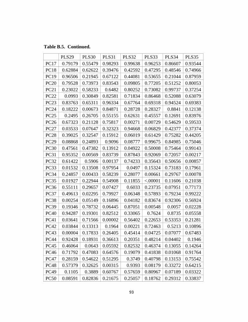
93



PC17 0.79179 0.55479 0.98293 0.99638 0.96253 0.86607 0.93544

PC18 0.62884 0.62622 0.39476 0.42592 0.47295 0.48546 0.74966

PC19 0.96506 0.21945 0.67122 0.44081 0.53655 0.21044 0.87959

PC20 0.79528 0.73973 0.83543 0.09805 0.77205 0.51252 0.80053

PC21 0.23022 0.58233 0.6482 0.80252 0.73082 0.99737 0.37254

PC22 0.0993 0.30849 0.82581 0.71834 0.86468 0.52088 0.63079

PC23 0.83763 0.65311 0.96334 0.67764 0.69318 0.94524 0.69383

PC24 0.18222 0.00673 0.84871 0.28728 0.28327 0.8841 0.12138

PC25 0.2495 0.26705 0.55155 0.62631 0.45557 0.12691 0.83976

PC26 0.67323 0.21128 0.75817 0.00271 0.00729 0.54629 0.59533

PC27 0.03533 0.07647 0.32323 0.94668 0.06829 0.42377 0.37374

PC28 0.39025 0.32547 0.15912 0.06019 0.61429 0.75282 0.44205

PC29 0.08868 0.24893 0.9096 0.08777 0.99675 0.84985 0.75046

PC30 0.47561 0.47382 0.13912 0.04922 0.50008 0.75464 0.99143

PC31 0.95352 0.00569 0.83739 0.87843 0.92069 0.72057 0.00217

PC32 0.61422 0.5906 0.00137 0.74233 0.35643 0.50656 0.00857

PC33 0.01532 0.13508 0.97954 0.0497 0.15324 0.73183 0.17961

PC34 0.24857 0.00433 0.58239 0.28077 0.00661 0.29767 0.00078

PC35 0.01927 0.22944 0.54908 0.11855 <.00001 0.11606 0.21038

PC36 0.55111 0.29657 0.07427 0.6033 0.23735 0.07951 0.77173

PC37 0.49613 0.02295 0.79927 0.06348 0.57893 0.79234 0.99222

PC38 0.00254 0.05149 0.16896 0.04182 0.83674 0.92306 0.56924

PC39 0.19346 0.78732 0.06445 0.87051 0.00548 0.0057 0.02228

PC40 0.94287 0.19301 0.82512 0.33065 0.7624 0.8735 0.05558

PC41 0.03641 0.71566 0.00002 0.56402 0.22653 0.53353 0.21281

PC42 0.03844 0.13313 0.1964 0.00221 0.72463 0.5213 0.10896

PC43 0.00004 0.17833 0.26405 0.45414 0.04725 0.07077 0.67483

PC44 0.92428 0.18931 0.36613 0.20351 0.48214 0.04402 0.1946

PC45 0.46064 0.0643 0.05592 0.82532 0.46374 0.13055 0.14264

PC46 0.71792 0.47083 0.64576 0.19079 0.41838 0.01068 0.91764

PC47 0.28159 0.54622 0.51295 0.3749 0.40798 0.13153 0.75542

PC48 0.57379 0.32625 0.00315 0.9393 0.08179 0.33272 0.64215

PC49 0.1105 0.3889 0.60767 0.57659 0.80967 0.07189 0.03322

PC50 0.08591 0.82836 0.21675 0.25057 0.18762 0.29312 0.33837

94



PC51 0.28534 0.67702 0.25263 0.41609 0.53632 0.62189 0.25261

PC52 0.79325 0.56848 0.88261 0.61447 0.55183 0.68888 0.01386

PC53 0.45499 0.6444 0.21767 0.19641 0.24185 0.04474 0.20922

PC54 0.44399 0.9806 0.19402 0.16866 0.76391 0.32233 0.37771

PC55 0.7942 0.84643 0.70261 0.49681 0.50965 0.24492 0.67826

PC56 0.5595 0.11889 0.28054 0.13812 0.08168 0.30889 0.91318

PC57 0.93345 0.45022 0.4567 0.04503 0.87029 0.51943 0.25161

PC58 0.71097 0.27953 0.78606 0.88297 0.18663 0.00714 0.70589

PC59 0.26367 0.94544 0.37326 0.46568 0.85987 0.56953 0.6871

PC60 0.95131 0.47171 0.82616 0.35756 0.79275 0.53297 0.62578

PC61 0.66894 0.39067 0.36068 0.29659 0.76904 0.87519 0.72326

PC62 0.89917 0.104 0.39592 0.007 0.62317 0.00696 0.85202

PC63 0.1829 0.9429 0.58375 0.57135 0.54628 0.58402 0.93539

PC64 0.8386 0.64018 0.73702 0.50492 0.7872 0.9248 0.80356

PC65 0.0516 0.35579 0.68577 0.29262 0.10297 0.22497 0.98401

PC66 0.70863 0.16021 0.91777 0.99588 0.78092 0.8833 0.53995

PC67 0.63801 0.49987 0.18122 0.58627 0.68019 0.83863 0.38664

PC68 0.75276 0.21142 0.61473 0.7323 0.8266 0.75585 0.5728

PC69 0.63866 0.30983 0.86884 0.33484 0.19757 0.72332 0.3098

PC70 0.98964 0.99522 0.4841 0.46826 0.9827 0.38246 0.40204

PC71 0.93539 0.40003 0.77857 0.8588 0.40094 0.19977 0.94395

PC72 0.771 0.06267 0.67012 0.1772 0.22131 0.3622 0.07675

PC73 0.98349 0.66835 0.56295 0.72632 0.60111 0.85615 0.10203

PC74 0.58581 0.99445 0.91174 0.90167 0.78389 0.86982 0.60848

PC75 0.35975 0.64164 0.15097 0.6784 0.78519 0.42312 0.08323

PC76 0.95974 0.33864 0.09714 0.98157 0.85406 0.74949 0.13764

PC77 0.18861 0.98532 0.95944 0.88765 0.56518 0.50755 0.60282

PC78 0.76474 0.7814 0.2361 0.66625 0.64674 0.19798 0.42447

PC79 0.65081 0.46886 0.65682 0.76411 0.63979 0.05425 0.97128

PC80 0.77138 0.94722 0.25643 0.83692 0.72725 0.8318 0.95058

PC81 0.92958 0.59531 0.23648 0.9713 0.90098 0.69513 0.90302

PC82 0.34205 0.32902 0.53913 0.51799 0.60402 0.86996 0.91721

PC83 0.82952 0.59191 0.5359 0.44022 0.4087 0.59125 0.92507

PC84 0.50642 0.34568 0.68171 0.84792 0.56253 0.27194 0.97239

PC85 0.53866 0.68013 0.34343 0.95238 0.69597 0.84689 0.9854

95



PC86 0.57604 0.51839 0.70422 0.93464 0.95455 0.76128 0.99682

PC87 0.91535 0.4902 0.50734 0.96572 0.78464 0.59385 0.53447

PC88 0.68108 0.98713 0.65973 0.24664 0.11761 0.58565 0.92005

PC89 0.4774 0.90864 0.67173 0.66575 0.54978 0.58748 0.78422

PC90 0.85164 0.95072 0.98984 0.8925 0.75737 0.60984 0.47188

PC91 0.95764 0.91537 0.79859 0.76405 0.70201 0.34946 0.85545

PC92 0.82337 0.70694 0.88491 0.95775 0.79871 0.50114 0.49063



PC1 0.89498 0.99572 0.98953 0.95684 0.97294 0.98998 0.9387

PC2 0.99333 0.94945 0.9714 0.99133 0.96728 0.90641 0.80642

PC3 0.96902 0.94276 0.99784 0.99931 0.9087 0.94177 0.95515

PC4 0.73018 0.95064 0.96721 0.88034 0.92462 0.8498 0.66531

PC5 0.77639 0.99934 0.90948 0.58324 0.9194 0.86947 0.82448

PC6 0.85845 0.92498 0.95325 0.84248 0.93496 0.90825 0.92515

PC7 0.94669 0.77275 0.94263 0.90063 0.94709 0.8464 0.96439

PC8 0.91268 0.76412 0.775 0.93544 0.87789 0.8653 0.97158

PC9 0.97287 0.83317 0.86522 0.97082 0.59797 0.97682 0.90952

PC10 0.79068 0.9184 0.92881 0.88946 0.96444 0.95586 0.8123

PC11 0.4676 0.60182 0.92095 0.73746 0.83048 0.97072 0.88652

PC12 0.54243 0.68314 0.92028 0.70966 0.86321 0.90882 0.83644

PC13 0.79724 0.94911 0.75651 0.87637 0.72906 0.90956 0.76306

PC14 0.84504 0.91415 0.87704 0.43341 0.95092 0.94991 0.88565

PC15 0.64468 0.75809 0.81252 0.89078 0.93905 0.96445 0.68498

PC16 0.78531 0.96826 0.89795 0.56074 0.40662 0.8203 0.55217

PC17 0.74782 0.77638 0.78917 0.82004 0.81356 0.86336 0.48155

PC18 0.57612 0.57434 0.48387 0.35204 0.68294 0.89454 0.19683

PC19 0.58559 0.60497 0.59673 0.33174 0.58716 0.64169 0.42803

PC20 0.73116 0.56147 0.60197 0.29814 0.65953 0.85136 0.12667

PC21 0.64538 0.96575 0.57368 0.28609 0.52947 0.99482 0.68954

PC22 0.86351 0.46058 0.75595 0.53841 0.90772 0.83755 0.81781

96



PC23 0.48521 0.69396 0.8239 0.58667 0.73071 0.6555 0.53812

PC24 0.32302 0.55523 0.74971 0.94435 0.71965 0.42958 0.68089

PC25 0.58775 0.71484 0.96657 0.86714 0.68379 0.69808 0.30806

PC26 0.52342 0.67905 0.13207 0.65318 0.78595 0.96072 0.78006

PC27 0.68271 0.92188 0.26098 0.16593 0.41317 0.95907 0.61258

PC28 0.32383 0.85489 0.92909 0.12155 0.44764 0.56628 0.54922

PC29 0.61339 0.48324 0.78035 0.51218 0.71936 0.56316 0.47283

PC30 0.14276 0.02251 0.72907 0.96558 0.54791 0.95307 0.96299

PC31 0.60354 0.28235 0.33932 0.20117 0.47139 0.30946 0.13677

PC32 0.81686 0.01155 0.96371 0.98177 0.3888 0.59434 0.54587

PC33 0.18038 0.01228 0.10433 0.33335 0.19799 0.54521 0.2322

PC34 0.17811 0.77684 0.59378 0.45921 0.62204 0.62561 0.92641

PC35 0.51013 0.30832 0.45295 0.61143 0.75613 0.52676 0.44002

PC36 0.27973 0.64594 0.06605 0.16136 0.37721 0.68314 0.61782

PC37 0.77987 0.01204 0.5273 0.82712 0.17556 0.70234 0.01052

PC38 0.25882 0.00242 0.26949 0.88962 0.0321 0.33536 0.03996

PC39 0.39768 0.86409 0.19424 0.54057 0.24553 0.13811 0.97374

PC40 0.02326 0.38603 0.02022 0.94339 0.86383 0.27504 0.76132

PC41 0.00401 0.42819 0.3168 0.29814 0.20799 0.49148 0.06248

PC42 0.79702 0.13814 0.24113 0.72642 0.57962 0.08288 0.51001

PC43 0.59283 0.03389 0.00495 0.91287 0.49135 0.57886 0.60329

PC44 0.76428 0.95376 0.44567 0.22781 0.76667 0.83274 0.05575

PC45 0.0039 0.15298 0.86675 0.16765 0.0714 0.07084 0.3735

PC46 0.54224 0.15474 0.03674 0.24047 0.00018 0.18221 0.542

PC47 0.87409 0.36238 0.64032 0.57646 0.82814 0.09917 0.30095

PC48 0.52818 0.21737 0.17065 0.29898 0.83966 0.63079 0.08713

PC49 0.03273 0.48767 0.02605 0.028 0.43257 0.28525 0.08507

PC50 0.73669 0.80009 0.82551 0.4993 0.03238 0.35904 0.30862

PC51 0.37294 0.49224 0.10087 0.34963 0.18701 0.04105 0.51779

PC52 0.00076 0.35743 0.1223 0.90253 0.54799 0.09004 0.11105

PC53 0.09866 0.56375 0.3445 0.45106 0.99051 0.85466 0.94236

PC54 0.04831 0.53028 0.37527 0.34159 0.82554 0.03436 0.64124

PC55 0.62879 0.09892 0.65104 0.03137 0.00706 0.19472 0.3459

97



PC56 0.23644 0.72134 0.04914 0.30643 0.99313 0.15856 0.59697

PC57 0.64559 0.9015 0.14974 0.98925 0.51423 0.56535 0.44663

PC58 0.58149 0.85151 0.14157 0.924 0.30455 0.002 0.85191

PC59 0.98418 0.69574 0.88937 0.72254 0.44536 0.84227 0.28356

PC60 0.88079 0.4882 0.76938 0.21148 0.06349 0.05516 0.03147

PC61 0.42573 0.47251 0.95251 0.00426 0.64982 0.02469 0.0977

PC62 0.79829 0.99667 0.38007 0.09839 0.06321 0.02639 0.37208

PC63 0.69293 0.45843 0.13459 0.06858 0.74496 0.91479 0.09433

PC64 0.54269 0.03668 0.66984 0.95523 0.55784 0.80513 0.13935

PC65 0.6039 0.84649 0.40252 0.8355 0.59969 0.90438 0.16979

PC66 0.56558 0.16866 0.85485 0.66581 0.25035 0.02299 0.00405

PC67 0.02183 0.14737 0.41636 0.60844 0.6679 0.0834 0.74365

PC68 0.80846 0.196 0.90284 0.03489 0.39514 0.8555 0.5361

PC69 0.71209 0.92742 0.28819 0.91437 0.43731 0.04518 0.86643

PC70 0.22479 0.42529 0.53406 0.08159 0.97991 0.52142 0.62311

PC71 0.5295 0.88583 0.3272 0.06755 0.06542 0.63077 0.59862

PC72 0.45869 0.84256 0.10665 0.54952 0.51824 0.83758 0.59531

PC73 0.19888 0.75045 0.33194 0.89268 0.81733 0.06756 0.93018

PC74 0.78055 0.13322 0.51757 0.06598 0.72404 0.83845 0.96964

PC75 0.6224 0.58262 0.81573 0.97288 0.95289 0.61923 0.14304

PC76 0.80663 0.4042 0.90628 0.95149 0.27858 0.61675 0.61665

PC77 0.23478 0.33089 0.60141 0.50277 0.79575 0.78356 0.86884

PC78 0.65701 0.13592 0.5099 0.02314 0.07526 0.66794 0.89864

PC79 0.13624 0.35051 0.42753 0.9531 0.41517 0.45505 0.99069

PC80 0.65723 0.588 0.61549 0.66475 0.56945 0.92583 0.68294

PC81 0.68681 0.90611 0.34216 0.7294 0.68709 0.80623 0.29241

PC82 0.76878 0.81808 0.95142 0.66493 0.53197 0.54678 0.84434

PC83 0.30908 0.40101 0.30597 0.06442 0.12758 0.20599 0.87855

PC84 0.22578 0.63958 0.01608 0.15299 0.67245 0.78245 0.7347

PC85 0.42526 0.24789 0.61705 0.65989 0.2698 0.94167 0.98078

PC86 0.50473 0.48389 0.86041 0.04969 0.32961 0.46284 0.83287

PC87 0.79133 0.75605 0.37503 0.86168 0.66149 0.7854 0.70087

PC88 0.58224 0.48062 0.57966 0.54628 0.09101 0.38165 0.27467

PC89 0.52343 0.29239 0.41498 0.69923 0.04254 0.85898 0.63646

PC90 0.09112 0.68547 0.18247 0.02603 0.32142 0.91523 0.85554

98



PC91 0.40226 0.95279 0.63796 0.34448 0.31973 0.04678 0.92862

PC92 0.29498 0.71272 0.10969 0.91371 0.10268 0.26506 0.54589


PLS43 PLS44 PLS45 PLS46 PLS47 PLS48

PC1 0.96926 0.93271 0.99325 0.99199 0.95816 0.9176

PC2 0.95959 0.99762 0.93565 0.96342 0.91612 0.79924

PC3 0.92519 0.90101 0.93397 0.92004 0.92683 0.98892

PC4 0.9888 0.80065 0.8967 0.96982 0.77011 0.59968

PC5 0.74592 0.86787 0.86444 0.97024 0.95699 0.95727

PC6 0.98643 0.95907 0.94654 0.96483 0.98147 0.82225

PC7 0.94825 0.99996 0.98843 0.95417 0.94654 0.99225

PC8 0.91628 0.96312 0.91591 0.88908 0.92229 0.87127

PC9 0.94228 0.96982 0.98786 0.99549 0.94788 0.92103

PC10 0.89243 0.77748 0.90101 0.94299 0.89436 0.96952

PC11 0.93374 0.85769 0.9117 0.97971 0.74627 0.74493

PC12 0.97029 0.79005 0.78056 0.9997 0.93416 0.95957

PC13 0.94149 0.97246 0.90568 0.95842 0.94897 0.9814

PC14 0.75314 0.8769 0.97636 0.98249 0.9082 0.89975

PC15 0.94204 0.96499 0.89685 0.8548 0.83163 0.78503

PC16 0.89052 0.69566 0.99708 0.70462 0.79992 0.43594

PC17 0.74615 0.67524 0.76618 0.81998 0.67946 0.61835

PC18 0.45389 0.3407 0.65704 0.86417 0.65995 0.7749

PC19 0.88842 0.43365 0.60256 0.69747 0.81099 0.49245

PC20 0.90713 0.36143 0.73559 0.86812 0.42558 0.71548

PC21 0.73347 0.34948 0.57019 0.99205 0.49882 0.94577

PC22 0.74602 0.89593 0.88814 0.75408 0.9304 0.86557

PC23 0.64575 0.68129 0.99561 0.99991 0.74955 0.85379

PC24 0.73416 0.81973 0.58885 0.91222 0.68708 0.5374

PC25 0.74844 0.88874 0.78135 0.59729 0.97212 0.49711

PC26 0.81262 0.47235 0.48647 0.89548 0.99554 0.86196

PC27 0.54881 0.17626 0.91626 0.76202 0.88155 0.54934

PC28 0.37147 0.54792 0.87458 0.78941 0.81433 0.82855

99



PC29 0.5167 0.65193 0.89851 0.71188 0.70265 0.59664

PC30 0.9527 0.62762 0.37868 0.22359 0.99908 0.47149

PC31 0.79637 0.39019 0.97074 0.30119 0.54135 0.60386

PC32 0.99275 0.42305 0.62178 0.53496 0.16799 0.6681

PC33 0.65573 0.90595 0.71061 0.91551 0.60611 0.31978

PC34 0.84163 0.60417 0.51821 0.24398 0.53251 0.24313

PC35 0.77115 0.185 0.72041 0.84814 0.96699 0.82955

PC36 0.93964 0.94617 0.08651 0.83792 0.49275 0.8804

PC37 0.46593 0.12046 0.21958 0.68716 0.47358 0.17091

PC38 0.40308 0.57625 0.98033 0.82419 0.64599 0.90653

PC39 0.87295 0.22128 0.09488 0.79976 0.71739 0.87737

PC40 0.38905 0.51597 0.51605 0.6243 0.09736 0.55459

PC41 0.91652 0.63799 0.41314 0.76611 0.57132 0.33258

PC42 0.97499 0.76106 0.33388 0.70094 0.9349 0.9895

PC43 0.06647 0.84828 0.63258 0.64852 0.439 0.19248

PC44 0.12985 0.39102 0.50973 0.14467 0.65635 0.49933

PC45 0.23321 0.8203 0.24672 0.21598 0.25602 0.10583

PC46 0.17581 0.90832 0.02839 0.82154 0.31037 0.35603

PC47 0.24208 0.12831 0.48185 0.59838 0.0362 0.02766

PC48 0.33587 0.934 0.13711 0.66775 0.38647 0.55721

PC49 0.25331 0.00011 0.60392 0.43797 0.03551 0.61355

PC50 0.3866 0.07159 0.13475 0.65131 0.04934 0.36586

PC51 0.0093 0.4198 0.19903 0.02046 0.82602 0.36718

PC52 0.21775 0.36736 0.1135 0.8204 0.0248 0.17183

PC53 0.83271 0.86162 0.28928 0.01029 0.80363 0.34811

PC54 0.19421 0.40885 0.14289 0.06303 0.5532 0.69428

PC55 0.2127 0.20786 0.4686 0.0164 0.0715 0.21636

PC56 0.52895 0.06202 0.91926 0.07302 0.57868 0.06763

PC57 0.01585 0.90067 0.26463 0.63516 0.04311 0.09922

PC58 0.42173 0.93484 0.04877 0.11457 0.08746 0.83694

PC59 0.05427 0.91007 0.85478 0.04669 0.31489 0.88761

PC60 0.00696 0.00465 0.73036 0.80149 0.82136 0.02116

PC61 0.51101 0.47154 0.92177 0.04052 0.12042 0.47769

PC62 0.58158 0.51663 0.00852 0.0922 0.39958 0.1041

100



PC63 0.00596 0.73364 0.49554 0.15513 0.74999 0.11587

PC64 0.30721 0.64956 0.0003 0.164 0.37588 0.11546

PC65 0.36213 0.00686 0.17034 0.12859 0.58588 0.73083

PC66 0.57271 0.1615 0.23787 0.03077 0.0388 0.46266

PC67 0.49527 0.22033 0.24935 0.66578 0.31115 0.36831

PC68 0.55478 0.11755 0.5123 0.67117 0.61016 0.35618

PC69 0.05763 0.95203 0.94253 0.68891 0.42872 0.68859

PC70 0.91373 0.73834 0.19272 0.44239 0.97049 0.79611

PC71 0.55956 0.99606 0.62288 0.43995 0.02491 0.68591

PC72 0.15698 0.84871 0.54645 0.51255 0.23655 0.54319

PC73 0.41642 0.71214 0.7181 0.24018 0.92293 0.86119

PC74 0.32287 0.06055 0.28875 0.33963 0.38777 0.13535

PC75 0.83892 0.00682 0.33709 0.17591 0.08817 0.49852

PC76 0.37531 0.4288 0.85617 0.01102 0.10276 0.87073

PC77 0.7171 0.2391 0.40182 0.7375 0.60733 0.29416

PC78 0.84502 0.00661 0.255 0.49556 0.39022 0.42139

PC79 0.75739 0.53107 0.28664 0.17032 0.15454 0.76421

PC80 0.91993 0.36755 0.63868 0.49517 0.46922 0.89826

PC81 0.96579 0.26442 0.76622 0.48659 0.89717 0.86502

PC82 0.27122 0.99633 0.79536 0.27483 0.86292 0.1718

PC83 0.92334 0.70729 0.92312 0.70365 0.94376 0.35801

PC84 0.3416 0.50637 0.58229 0.88966 0.54057 0.13952

PC85 0.37955 0.6005 0.748 0.56421 0.26493 0.78494

PC86 0.77418 0.8553 0.68554 0.32714 0.56999 0.12469

PC87 0.1246 0.49987 0.62072 0.21232 0.28375 0.10585

PC88 0.56382 0.80193 0.32124 0.75658 0.36619 0.08194

PC89 0.6065 0.84463 0.71992 0.30087 0.40522 0.99176

PC90 0.78569 0.61063 0.97797 0.11454 0.18097 0.1057

PC91 0.56418 0.64101 0.62879 0.99325 0.80236 0.46765

PC92 0.27382 0.40035 0.91522 0.0137 0.00201 0.00557

101

BIBLIOGRAPHY

Albanese, J. (2003) A metric method for sex determination using the hipbone and the

femur. Journal of Forensic Sciences 48:1-11.

Anderson, B. E. (1990) Ventral arc of the os pubis: Anatomical and developmental

considerations. American Journal of Physical Anthropology 83:449-458.

Baker, B. J., T. L. Dupras, and M. W. Tocheri (2005) The Osteology of Infants and

Children. Texas A&M University Press, College Station, TX.

Bass, W. M. (2005) Human Osteology: A Laboratory and Field Manual, pp. 19-21.

Missouri Archaeological Society, Columbia, MO.

Bastir, M., P. Godoy., and A. Rosas (2011) Common features of sexual dimorphism in

the cranial airways of different human populations. American Journal of Physical

Anthropology 146:414-422.

Bookstein, F. L. (1991) Morphometric Tools for Landmark Data: Geometry and Biology.

Cambridge University Press, Cambridge.

Bookstein, F. L. (1997) Landmark methods for forms without landmarks: Morphometrics

of group differences in outline shape. Medical Image Analysis 1:225-243.

Budinoff, L. C. and R. G. Tague (1990) Anatomical and developmental bases for the

ventral arc of the human pubis. American Journal of Physical Anthropology

82:73-79.

Buikstra, J. E. and D. H. Ubelaker (1994) Standards for Data Collection from Human

Skeletal Remains. Arkansas Archaeological Survey, Fayetteville, AK.

Bytheway, J. A. (2003) Sex determination of the adult human fragmented pelvis utilizing

Euclidean distance matrix analysis. Ph.D. thesis. University of Pittsburgh,

Pittsburgh, PA.

Bytheway, J. A. and A. H. Ross (2010) A Geometric morphometric approach to sex

determination of the human adult os coxa. Journal of Forensic Sciences 55:859-

864.

Cole, T. M. III (1996) Historical note: Early anthropological contributions to “Geometric

Morphometrics.” American Journal of Physical Anthropology 101:291-296.

Coleman, W. H. (1969) Sex differences in the growth of the human bony pelvis.

American Journal of Physical Anthropology 31:125-151.

102

Cramon-Taubadel, N., B. C. Frazier, and M. M. Lahr (2007) The problem of assessing

landmark error in geometric morphometrics: Theory, methods, and modifications.


Cunningham, F. G. and J. W. Williams (2005) Williams Obstetrics (22nd

ed.). McGraw-

Hill, New York.

Daubert v. Merrell Dow Pharmaceuticals Inc., 113S.Ct.2786 (1993).

Diamond-Smith, N. and M. Potts (2011) A woman cannot die from a pregnancy she does

not have. International Perspectives on Sexual and Reproductive Health 37:155-

158.

Ellison, P. T. (2001) On Fertile Ground. Harvard University Press, Cambridge.

Ellison, P. T. (2008) Energetics, reproductive ecology, and human evolution.

Paleoanthropology 172-200.

Frutos, L. R. (2002) Determination of sex from the clavicle and scapula in a Guatemalan

contemporary rural Indigenous population. American Journal of Forensic

Medicine & Pathology 23:284-288.

Giles, E. and O. Elliot (1963) Sex determination by discriminant function analysis of

crania. American Journal of Physical Anthropology 21:53-68.

Goldsmith, L. T. and G. Weiss (2009) Relaxin in human pregnancy. Annals of the New

York Academy of Sciences 1160:130-135.

González, P. N. (2005) Variabilidad poblacional en rasgos dimórficos de la pelvis:

Implicancias en la estimación del sexo de individuos adultos. Revista Argentina

de Antropología Biológia 7:120.

González, P. N., V. Bernal, S. I. Perez and G. Barrientos (2007) Analysis of dimorphic

structures of the human pelvis: Its implications for sex estimation in samples

without reference collections. Journal of Archaeological Science 34:1720-1730.

González, P. N. V. Bernal, and S. I. Perez (2009) Geometric morphometric approach to

sex estimation of human pelvis. Forensic Science International 189:68-74.

González, P. N. V. Bernal, and S. I. Perez (2011) Analysis of sexual dimorphism of

craniofacial traits using geometric morphometric techniques. International

Journal of Osteoarchaeology 21:82-91.

Greulich, W. W. and H. Thoms (1944) The growth and development of the pelvis of

individual girls before, during, and after puberty. Yale Journal of Biology and

Medicine 17:91-98.

103

Hunt, D. R. and J. Albanese (2005) History and demographic composition of the Robert

J. Terry Anatomical Collection. American Journal of Physical Anthropology

127:406-417.

Hogan, M. C, K. J. Foreman, M. Naghavi, S. Y. Ahn, M. Wang, S. M. Makela, A. D.

Lopez, R. Lozano, and C. J. Murray (2010) Maternal mortality for 181 countries,

1980-2008: a systematic analysis of progress towards Millennium Development

Goal 5. Lancet 375:1609-1623.

IBM Corporation (2011) IBM SPSS Statistics for Windows, Version 20.0. Armonk, NY:

IBM Corp.

Immersion Corporation (2008) Microscribe Utility Software.

İşcan, M. Y. and P. Miller-Shaivitz (1986) Sexual dimorphism in the femur and tibia. In:

Forensic Osteology: Advances in the Identification of Human Remains, pp. 101-

111, ed. by K. J. Reichs, Charles C. Thomas, Springfield, IL.

Johnson, M. R., A. A. Abbas, A. C. Allman, K. H. Nicolaides, and S. L. Lightman (1994)

The regulation of plasma relaxin levels during human pregnancy. Journal of

Endocrinology 142:261-265.

Kerley, E. R. (1977) Forensic anthropology. In Forensic Medicine: A Study in Trauma

and Environmental Hazards: Vol. II ed. by C. G. Tedeschi, W. G. Eckert, and L.

G. Tedeschi, pp. 1101-1115. W.B. Saunders Co, Philadelphia.

Kimmerle, E. H., R. L. Jantz, L. W. Konigsberg, and J. P. Baraybar (2008) Skeletal

estimation and identification in American and East European populations.

Journal of Forensic Sciences 53:524-532.

Klales, A. R., S. D. Ousley, and J. M. Vollner (2012) A revised method of sexing the

human innominate using Phenice’s nonmetric traits and statistical methods.


Klingenberg, C. P. (2008) Morphological integration and developmental modularity.

Annual Review of Ecology, Evolution and Systematics 39:115-132.

Klingenberg, C. P. (2009) Morphometric integration and modularity in configurations of

landmarks: Tools for evaluating a priori hypotheses. Evolution and Development

11:405-421.

Klingenberg, C. P. 2011. MorphoJ: an integrated software package for geometric

morphometrics. Molecular Ecology Resources 11: 353-357.

Klingenberg, C. P. and L. R. Monteiro (2005) Distances and directions in

multidimensional shape spaces: Implications for morphometric applications.

Systematic Biology 54:678-688.

104

Klingenberg, C. P. and S. D. Zaklan (2000) Morphological integration between

developmental compartments in the Drosophila wing. Evolution 54:1273-1285.

Kurki, H. K. (2007) Protection of obstetric dimensions in a small-bodied human sample.

American Journal of Physical Anthropology 133: 1152-1165.

Kurki, H. K. (2011) Pelvic dimorphism in relation to body size and body size

dimorphism in humans. Journal of Human Evolution 61:631-643.

Kurki, H. K. (2011b) Compromised skeletal growth? Small body size and clinical

contraction thresholds for the female pelvic canal. International Journal of

Paleopathology 1:138-149.

Kurki, H. K. (2013) Bony pelvic canal size and shape in relation to body proportionality

in humans. American Journal of Physical Anthropology 151:88-101.

Kuzawa, C. W. (1998) Adipose tissue in human infancy and childhood: an evolutionary

perspective. Yearbook of Physical Anthropology 27:177-209.

Leary, S., C. Fall, C. Osmond, H. Lovel, D. Campbell, J. Eriksson, T. Forrester, K.

Godfrey, J. Hill, M. Jie, C. Law, R. Newby, S. Robinson, and C. Yajnik (2006)

Geographical variation in neonatal phenotype. Acta Obstetricia et Gynecologica

Scandinavica 85:1080-1089.

Lele, S. & J. Richtsmeier (2001) An Invariant Approach to Statistical Analysis of Shapes.

Chapman and Hall/CRC, Boca Raton, FL.

Listi, G. A. (2010) The impact of racial metric variation in the os coxae on the

morphological assessment of sex. Journal of Forensic Sciences 55:1157-1161.

Loth, S. R. and M. Henneberg (1996) Mandibular ramus flexure: A new morphologic

indicator of sexual dimorphism in the human skeleton. American Journal of

Physical Anthropology 99:473e83.

McLaughlin, S. M. and M. F. Bruce (1990) The accuracy of sex identification in

European skeletal remains using the Phenice characters. Journal of Forensic

Sciences 35:1384-1392.

Mittler, D. M. and S. G. Sheridan (1992) Sex determination in subadults using auricular

surface morphology: A forensic science perspective. Journal of Forensic

Sciences 37:1068-1075.

Oettlé, A. C., E. Pretorius, and M. Steyn (2005) Geometric morphometric analysis of

mandibular ramus flexure. American Journal of Physical Anthropology 128:623-

629.

Oxorn, H. (1986) Human Labor and Birth. Appleton Century-Crofts, New York.

105

Phenice, T. W. (1969) A newly developed visual method for sexing the os pubis.


Pretorius, E., M. Steyn, and Y. Scholtz (2006) Investigation into the usability of

geometric morphometric analysis in assessment of sexual dimorphism. American

Journal of Physical Anthropology 129:64-70.

Purkait, R. (2005) Triangle identified at the proximal end of femur: A new sex

determinant. Forensic Science International 147:135-139.

Reynolds, E. (1945) The bony pelvic girdle in early infancy. A roentgenometric study.


Richtsmeier, J. T., V. B. DeLeon, and S. R. Lele (2002) The promise of geometric

morphometrics. Yearbook of Physical Anthropology 45:63-91.

Rissech, C. and A. Malgosa (2007) Pubis growth study: Applicability in sexual and age

diagnostic. Forensic Science International 173:137-145.

Rogers, T. L. (1999) A visual method of determining the sex of skeletal remains using the

distal humerus. Journal of Forensic Sciences 44:57-60.

Rogers, N. L., L. E. Flournoy, and W. F. McCormick (2000) The rhomboid fossa of the

clavicle as a sex and age estimator. Journal of Forensic Sciences 45:61-67.

Rohlf, F. J. and D. E. Slice (1990) Extensions of the Procrustes method for the optimal

superimposition of landmarks. Systematic Zoology 39:40-59.

Ruff, C. B. (1991) Climate, body size and body shape in hominid evolution. Journal of

Human Evolution 21:81-105.

Ruff, C.B. (1994) Morphological adaptation to climate in modern and fossil Hominids.

Yearbook of Physical Anthropology 37:65-107.

Saini, V., R. Srivastava, S. N. Shamal, T. B. Singh, A. K. Pandey, and S. K. Tripathi

(2011) Sex determination using mandibular ramus flexure: A preliminary study

on Indian population. Journal of Forensic and Legal Medicine 18:208-212.

Saunders, S. R. and R. D. Hoppa (1997) Sex allocation from long bone measurements

using logistic regression. Canadian Society of Forensic Science Journal 30:49-

50.

Scheuer, L. and S. Black (2000) Developmental Juvenile Osteology. Elsevier Academic

Press, San Diego, CA.

Seidler, H. (1980) Sex-diagnosis of isolated os coxae by discriminant functions. Journal

of Human Evolution 9:597-600.

106

Slice, D. E. (2005) Modern Morphometrics. In Modern Morphometrics in Physical

Anthropology ed. by D. E. Slice, pp. 1-45. Kluwer Academic, New York.

Slice, D. E. (2007) Geometric Morphometrics. Annual Review of Anthropology 36:261-

281.

Slice, D. E. and A. Ross (2009) 3D-ID: Geometric morphometric classification of crania

for forensic scientists. http://www.3d-id.org.

Sneath, P. H. (1967) Trend-surface analysis of transformation grids. Journal of Zoology

151:65-122.

Spradley, M. K. and R. L. Jantz (2011) Sex estimation in forensic anthropology: Skull vs.

postcranial elements. Journal of Forensic Sciences 56:289-296.

Steudel, K. (1981) Sexual dimorphism and allometry in primate ossa coxae. American


Stewart, T. D. (1956) Examination of the possibility that certain skeletal characters

predispose to defects in the lumbar neural arches. Clinical Orthopedics 8:44-60.

Steyn, M., E. Pretorius, and L. Hutten (2004) Geometric morphometric analysis of the

greater sciatic notch in South Africans. HOMO 54:197-206.

Steyn, M. and M. L. Patriquin (2009) Osteometric sex determination from the pelvis-

Does population specificity matter? Forensic Science International 191:113.e1-

113.e5.

Sutter, R. C. (2003) Nonmetric subadult skeletal sexing traits: I. A blind test of the

accuracy of eight previously proposed methods using prehistoric known-sex

mummies from Northern Chile. Journal of Forensic Sciences 48:1-9.

Tague, R. G. (2000) Do big females have big pelves? American Journal of Physical


Tague, R. G. (2005) Big-bodied males help us recognize that females have big pelves.


Todd T. W. (1920) Age changes in the pubic bones. I: The White male pubis. American


Todd, T. W. (1921) Age changes in the pubic bone. II: The pubis of the male Negro-

White hybrid, III: The pubis of the White female, IV: The pubis of the female

Negro-White hybrid. American Journal of Physical Anthropology 4:1-70.

Ubelaker, D. H. & C. G. Volk (2002) A test of the Phenice method for the estimation of

sex. Journal of Forensic Sciences 47:19-24.

http://www.3d-id.org/

107

Valeri, C. J., T. M. Cole, S. Lele, and J. T. Richtsmeier (1998) Capturing data from three-

dimensional surfaces using fuzzy landmarks. American Journal of Physical


Vance, L. V., M. Steyn, and E. N. L’Abbé (2011) Nonmetric sex determination from the

distal and posterior humerus in Black and White South Africans. Journal of Forensic Sciences 56:710-714.

Walker, P. L. (2005) Greater sciatic notch morphology: Sex, age, and population

differences. American Journal of Physical Anthropology 127:385-391.

Walker, P. L. (2008) Sexing skulls using discriminant function analysis of visually

assessed traits. American Journal of Physical Anthropology 136:39-50.

Washburn, S. L. (1948) Sex differences in the pubic bone. American Journal of Physical


Washburn, S. L. (1960) Tools and human evolution. Scientific American 203:63-75.

Wells, C. (1975) Ancient obstetric hazards and female mortality. Bulletin of the New

York Academy of Medicine 51:1235-1249.

Wells, J. C., J. M. DeSilva and J. T. Stock (2012) The obstetric dilemma: An ancient

game of Russian roulette, or a variable dilemma sensitive to ecology? Yearbook of

Physical Anthropology 55:40-71.

White, T. D. (2000) Human Osteology (2nd

ed.). Academic Press, San Diego.

White, T. D. and P. A. Folkens (2005) The Human Bone Manual. Elsevier, Burlington,

MA.

Wienker, C. W. (1984) Sex determination from human skeletal remains: A case of a

mistaken assumption. In Human Identification: Case Studies in Forensic

Anthropology ed. by T. A. Rathbun & J. E. Buikstra, pp. 229-241. Charles C.

Thomas, Springfield, IL.

Wilson, L. A., N. MacLeod, and L. T. Humphrey (2008) Morphometric criteria for

sexing juvenile human skeletons using the ilium. Journal of Forensic Sciences

53:269-278.

108

CURRICULUM VITAE

Brianne E. Charles

1987

[email protected]

3251 Normandy Lane

Green Bay, WI 54301

Education Masters of Science Degree in Forensic Anthropology

(In progress)

Boston University School of Medicine, Boston, MA.

(GPA 3.9)

Graduate Coursework

Osteology and Anatomy

Outdoor Crime Scene Investigation

Forensic Taphonomy

Forensic Anthropology Techniques

Pathology

Experimental Design

Biostatistics

Advanced Human Osteology

Mortuary Archaeology

History, Method, and Theory in Biological

Anthropology

Forensic Anthropology Field Methods

Bioarchaeology

Applied Forensic Anthropology

Expert Witness Testimony

Sept

2013

Bachelors of Arts Degree in Anthropology

University of WI-Milwaukee, Milwaukee, WI.

Dean’s List 3 semesters (GPA 3.495)

May

2010

Research

Experience

Boston University School of Medicine Department of

Anatomy and Neurobiology, Forensic Anthropology Program Boston, MA.

Advisor: Mr. Jonathon Bethard, MA

Thesis Title: “A Geometric Morphometric Analysis

of the Human Ossa Coxae for Sex Estimation”

2011-

2013

mailto:[email protected]

109

Related

Training

and

Experience

Analysis of Organismal Form, University of

Manchester, Manchester, UK

Online course taught by Christian Klingenberg

with focus on geometric morphometric analysis

and the use of MorphoJ software in various

biological fields

Fall 2012

Knoxville Regional Forensic Center, Knoxville, TN

Worked under the supervision of Dr. Murray K.

Marks

Processed bodies for the collection of skeletal

remains

July 2012

Ecomuseu de Cap de Cavalleria Field School,

Menorca, Spain

Participated in the excavation of a tomb at a

Roman necropolis

Analyzed and documented skeletal remains in

laboratory

Prepared a final presentation on taphonomic factors

affecting the condition of skeletal remains

May-

June

2012

Forensic Entomology Seminar, Boston University

School of Medicine, Boston, MA

Attended lecture by Dr. Ian Dadour from the

University of Western Australia on the applications

of entomology within a forensic setting and current

research in the field

March

2012

Archival Project for the Milwaukee County

Institutional Grounds Cemetery, University of WI- Milwaukee, Milwaukee, WI

Documented and packaged skeletal remains from

an historical cemetery

Applied methods of archival consistent with

project protocol

February

2009- May

2010

110

Zooarchaeology Study Abroad Course, University

of WI-Milwaukee, Huanchaco, Peru

Emphasis on Moche culture and zooarchaeology in

the North Coast region of Peru

Sorted, identified, catalogued, and bagged faunal

June

2009

remains

Relevant

Training

Microscribe® Digitizer

Leica Total Station

TDS Recon Data Logger and Survey Pro

FEMA NIMS Incident Command System: ICS-

100 Level

Maceration of Human remains

Computer programs: FORDISC 3.0, MorphoJ,

Microsoft Excel

A Geometric Morphometric Analysis of the Human Ossa Coxae for Sex Determination

Documents

Transcript of A Geometric Morphometric Analysis of the Human Ossa Coxae for Sex Determination