A geometric approach to subpixel registration accuracy

COMPUTER VISION, GRAPHICS, AND IMAGE PROCESSING 40 , 3 3 4 - 3 6 0 (1987)

A Geometric Approach to Subpixel Registration Accuracy

CARLOS A. BERENSTEIN,* LAVEEN N. KANAL,* DAVID LAVINE, AND ERIC C. OLSON

L. N. K. Corporation, Suite 306, 6811 Kenilworth Ave., Riverdale, MD 20737

Received November 11, 1984; accepted March 5, 1987

A method for estimating the translation offset between a pair of images to subpixel accuracy is described and analyzed. This method assumes the extraction of a digital edge representing a straight line in the image and then computes the best real line which could have given rise to the digital line. The key difference between this method and other approaches to subpixel fitting is that our method uses subpixel line location to estimate a digital model such as the digital line and then fits the digital model to the image while other approaches directly fit a continuous model to the image or an image related object such as a cross correlation matrix. The present paper lays a theoretical foundation for this digital approach. This technique can be applied in a variety of remote sensing and industrial vision problems requiring subpixel registration accuracy. �9 1987 Academic Press, Inc.

1. INTRODUCTION TO GEOMETRIC REGISTRATION

Matching edges in sensed and reference images can be used for registration. The degree to which the position of a real-world edge, such as a field boundary, can be located in imagery depends heavily upon one's knowledge of the scene and the sensors. Edge detectors can be used to locate reasonable candidates for edge points and then an edge can be more precisely fit using these points. Alternatively, an estimate of subpixel edge location can be formed directly from the grey levels [5]. Hybr id approaches may also be adapted. We study the accuracy attainable using the first of these approaches, which we call the geometric accuracy approach.

Before launching into a description of our model for geometric accuracy, it is useful to consider those aspects of the registration problem we wish to capture in our model. The heart of our approach is to estimate the position of an image edge to subpixel accuracy and use this information to define a translation between the sensed and the reference image. In the ideal case, the grey levels on each side of the edge are constant off the edge pixels and the edge pixel grey levels are a simple weighted average o f these two grey levels. If all grey levels are possible and the edge pixels are all known then the position of the edge can be exactly determined by solving a system of linear equations expressing the observed grey levels as a function of the edge parameters. Such a situation is clearly unrealistic but it serves as a starting point for approximation.

Most current methods for attaining subpixel accuracy employ some type of interpolation of the correlation function. If such a method is to achieve subpixel accuracy, the digital correlation function must be able to achieve pixel accuracy. In

*University of Maryland; partially supported by NSF grants.

334 0734-189X/87 $3.00 Copyright �9 1987 by Academic Press, Inc. All rights of reproduction in any form reserved.

SUBPIXEL REGISTRATION ACCURACY 335

our work, we assume pixel accuracy is available either through correlation or other methods. Thus, in the simple case of a one-dimensional shif t any real world point can be determined to fie within a 3 • 1 pixel strip. Our results can be improved drastically if we assume we know, from registration, we are in the correct pixel, but this is a highly unrealistic assumption.

The analysis described in this paper pertains to the problem of one-dimensional translations. For long fines this is not particularly restrictive since the two-dimensional problem can be easily decomposed into one-dimensional shift estimates. In the line location estimation problem, we are trying to locate a real world line y = m x + b in the image. A shift (Ax, Ay) between real world and image coordinates yields a line y = m ( x - A x ) + b + A y in the image. This may be written as y = m x + b + ( A y - m Ax) which is the original fine shifted only in the y direction and by an amount y " m Ax, when the line is infinite.

Our I - d estimation procedures enable us to estimate Ay - m Ax. Given two lines, we can solve (possibly using least squares) for Ax and Ay separately. From this point on, we will confine ourselves to 1 - d shifts.

The models described here assume a set of pixels labelled edge pixels are provided by an edge detection procedure. Three cases can be considered. First, the set of edge pixels are exactly the digital edge corresponding to a fine in the real world. This model is unduly restrictive since an edge which comes very near a pixel boundary can show up in the next pixel due to noise. Second, one could consider a model in which the set of edge pixels given is a subset of the digital edge corresponding to the real edge. This approach is more realistic since it enables us t o discard some pixels whose classification as edge pixels is in doubt. Finally, we could give a model in which some pixels lying on the digitization of the real edge are given and some incorrect pixels are given.

For the first model, in which a complete digital edge is available, a tight upper bound for the registration error as a function of the line parameters is given (Section 3). This allows us to give some probabilistic error estimates for the family of all digital lines (Section 7). This analysis provides the firm basis for the study of the second and third models, but since our results in these cases are not so complete yet, we leave them to future reports. We notice nevertheless that in many applications one only finds rather short digital fines, with information only on 10 to 20 pixels, and hence occasionally, e.g., if no analytic formulas are available, it might be perfectly justified to rely on computer-aided counting of possibilities when this counting is not too time consuming.

As a first step in our analysis we parametrize the chain codes of digital fines see (Section 2 for definitions) by four parameters N, q, p, s as proposed by [2] and use some formulas from the same paper. We present alternate proofs in Appendix A. There is an excellent report [8] which seems to be generally unnoticed, and where there are several characterizations of those chain codes corresponding to digital lines among all possible strings of O's and l's. We do not use their results explicitly but they seem essential in the analytic study of the second and third models. We point out that both in [2, 8] as in other work in the literature, no attention is paid to the counting of all digital fines of finite length. It is not enough to count lines through the origin as done in [8] and since our probabilistic analyses require such count, we give an exact formula for the number of all fines in Section 6, which is not a straightforward generalization of the formula for fines through the origin. We also

336 BERENSTEIN ET AL.

provide asymptotic bounds for the number of lines of a given length as well as provide grounds for the reasonable conjecture that this number L ( N ) is of the form

L ( N ) = N3/~r 2 + O ( N Z l o g N ) .

A proof of this conjecture will appear shortly. A brief outline of the notation used is found in Appendix B.

2. DIGITAL STRAIGHT LINE SEGMENT PARAMETER ESTIMATION

Estimation of the location parameters of a real world edge giving rise to an image edge is discussed in this section. The ideas discussed are a summary of those parts of [2] which are useful for subpixel registration. Their basic result is a determination of all lines whose digitization is a specified chain code. In later sections, this set of lines will be used to derive error bounds on registration accuracy.

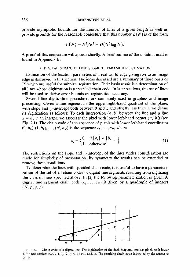
Several line digitization procedures are commonly used in graphics and image processing. Given a line segment in the upper right-hand quadrant of the plane, with slope and y-intercept both between 0 and 1 and strictly less than 1, we define its digitization as follows: To each intersection (a, b) between the line and a line x = a, a an integer, we associate the pixel with lower left-hand comer (a, tbl) (see Fig. 2.1). The chain code of the sequence of pixels with lower left-hand coordinates (0, bo), (1, bx) . . . . , ( N, bN) is the sequence Cl, . . . , c N, where

c , = {01 if[bi]=[b'-l])otherwise. (1)

The restrictions on the slope and y-intercept of the lines under consideration are made for simplicity of presentation. By symmetry the results can be extended to remove these conditions.

To determine the lines with specified chain code, it is useful to have a parameterization of the set of all chain codes of digital line segments resulting from digitizing the class of lines specified above. In [2] the following parameterization is given. A digital line segment chain code (c I . . . . , CN) is given by a quadruple of integers ( N , p , q , s ) .

J v - -

~176 0

FIG. 2.1. Chain code of a digital line. The digitization of the dark diagonal line has pixels with lower left-hand vertices (0, 0), (1,0), (2, 0), (3,1), (4, 1), (5,1). The resulting chain code indicated by the arrows is 00100.


N is the length of the chain code, i.e., the number of O's and l's. We note that not every string of O's and l ' s is generated by a line segment. For a characterization of those that are, see [10].

Next q is defined to be the smallest integer such that there exists an extension cN+l, cN+2, . . . , with Cl, C2, c3, . . , periodic with period q. Define p to be the number of ones in a period. The fourth parameter, s, provides a normalization of the chain code for one period. Geometrically, s may be interpreted as follows. Any chain code corresponds to a line segment with rational slope. Among all such segments, select the slope p / q with p A q = 1 which has the minimum q. This q is the period. The standard chain code corresponding to the first period of this chain code is the chain code of the digitization of the first q pixels of the line through the origin, y = ( p / q ) x . The ith element ci, of this chain code is given by

c i = [ i ( p / q ) ] - [ ( i - 1 ) ( p / q ) ] , i = 1,2 . . . . . N

The parameter s, of a code string of length N, is defined by the condition that the standard code string of p / q starts at the (s + 1)th element of the original chain code. Given the parameters N, q, p, s of a codestring, the ith element of the original code string can be obtained by

ci = l(i - s)(p/q)l - t(i - s - 1 ) ( p / q ) ] , i = 1,2 . . . . . N

The parameters satisfy the constraints 0 < p < q < N and 0 < s < q - 1. A point which will be particularly important for the registration problem is that there are constraints on the parameters other than the above inequalities. These additional constraints are described in Appendix A. Our interest in these matters stems from the need to enumerate the digital lines satisfying various conditions. If it were not for these messy constraints, the enumeration problems would often be straightforward. Without these additional constraints for fixed N, we would obtain all digital line segments of length N by independently varying s, p, and q subject to the c o n s t r a i n t s 0 < p < q < N a n d 0 < s < q - 1 .

We now give an example of the computation of the parameters for a chain code.

EXAMPLE. Chain code 10010100

N = 8: there are 8 digits in the code

q = 5: the above code is part of the infinite code 100101001010010...

p = 2: the number of l 's in the period 10010 is 2

s = 1: the standard codestring of ~ is 00101. The standard codestring starts at the 2nd element of the chain code. Hence s = 1.

The primary result of [2] is a description of the set of all lines whose digitization over the interval [0, N] is a set of pixels specified by a chain code. This result is of great importance for our registration accuracy results since it provides a hold on the errors which may arise by approximating the true edge by a feasible edge. The set of lines is described by a quadrilateral in the (e, a)-plane, where e is the y-intercept of


a line and a is the slope. We will call this plane the dual plane. The proof of the following formulas will be found in Appendix A.

Define functions F and L by

F(s ) = s - [s /q]q (2)

and

L ( s ) = s + [(N - s ) / q l q (3)

Let l be defined by the equation:

1 + [ l (p /q )] - l ( p / q ) = 1/q and 0 < l < q, (4)

or, what is the same, by the fact that lp = - 1 (mod q). The set of feasible lines is a convex quadrilateral in (e, a)-space with vertices A, B, C, D given by

A = ( [ r ( s ) p / q ] - r ( s ) p + / q +, p+/q+)

B = ( [ F ( s ) p / q ] - r ( s ) p / q , p / q )

C = (1 + [ r ( s + l )p /q ] - F(s + l ) p / q , p / q )

D = (1 + [ r ( s + l ) p / q ] - F(s + l ) p - / q - , p - / q - ) ,

where

(5) (6) (7) (8)

q+= L ( s + l) - F(s ) , p+ = (pq+ + l ) / q (9)

q - = L ( s ) - F ( s + l ) , p - = ( p q - - 1 ) / q . (10)

The above expressions for the vertices of the feasible quadrilateral will be discussed in greater detail in later sections. We note that neither of the vertices A, C, D, nor the points in the two sides of the quadrilateral determined by them correspond to lines that have the chain code (N, q, p, s) after digitization.

PROPOSITION 1. The formulas (2)-(10) defining the quadrilateral A, B, C, D are correct and furthermore q+ > O, q- > O, p+ > O, and p - > O.

3. FEASIBLE REGION SHAPE

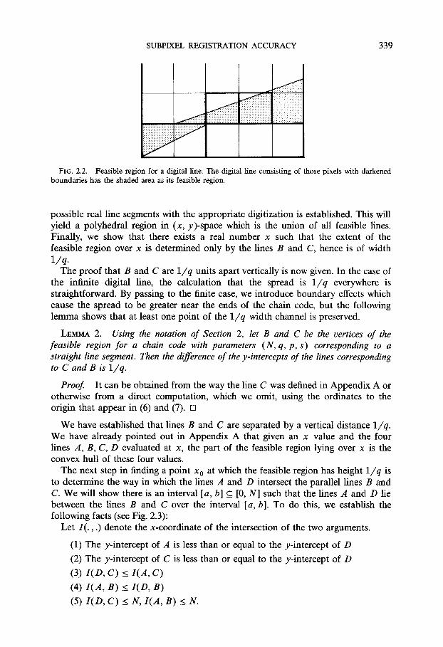
The description of the set of all lines whose digitization is a specified chain code of a straight line segment will now be used to obtain a worst-case bound on the subpixel accuracy with which we can locate a point in the image. We will show that given a period q chain code of the digitization of a straight line segment, there exists a real number x such that the total spread on y-values at the point x of all line segments with the given chain code is 1/q (see Fig. 2.2). Thus by selecting the midline of this set, the error is bounded by 1/(2q). This provides our error bound. In Section 4, we will examine the distribution of 1/(2q) corresponding to a probability distribution on lines.

To see the correctness of the 1/q spread, we first observe that the parallel lines B and C of the feasible region (Section 2) have slope p/q . We show that the vertical separation is 1/q. These lines may be thought of as providing a channel where we can find x values where the spread is 1/q. Next, the relationship between the location of the feasible region vertices in (e, a)-space and the location of points on


. iiii I FIG. 2.2. Feasible region for a digital line. The digital line consisting of those pixels with darkened

boundaries has the shaded area as its feasible region.

possible real line segments with the appropriate digitization is established. This will yield a polyhedral region in (x, y)-space which is the union of all feasible lines. Finally, we show that there exists a real number x such that the extent of the feasible region over x is determined only by the lines B and C, hence is of width 1/q.

The proof that B and C are 1/q units apart vertically is now given. In the case of the infinite digital line, the calculation that the spread is 1/q everywhere is straightforward. By passing to the finite case, we introduce boundary effects which cause the spread to be greater near the ends of the chain code, but the following lemma shows that at least one point of the 1/q width channel is preserved.

LEMMA 2. Using the notation of Section 2, let B and C be the vertices of the feasible region for a chain code with parameters (N, q, p, s) corresponding to a straight line segment. Then the difference of the y-intercepts of the lines corresponding to C and B is 1/q.

Proof It can be obtained from the way the line C was defined in Appendix A or otherwise from a direct computation, which we omit, using the ordinates to the origin that appear in (6) and (7). []

We have established that lines B and C are separated by a vertical distance 1/q. We have already pointed out in Appendix A that given an x value and the four lines A, B, C, D evaluated at x, the part of the feasible region lying over x is the convex hull of these four values.

The next step in finding a point x 0 at which the feasible region has height 1/q is to determine the way in which the lines A and D intersect the parallel lines B and C. We will show there is an interval [a, b] ___ [0, N] such that the lines A and D lie between the lines B and C over the interval [a, b]. To do this, we establish the following facts (see Fig. 2.3):

Let I ( . , .) denote the x-coordinate of the intersection of the two arguments.

(1) The y-intercept of A is less than or equal to the y-intercept of D

(2) The y-intercept of C is less than or equal to the y-intercept of D

(3) I(O, C) < I(A, C)

(4) I(A, B) < I(D, B) (5) I(D, C) < N, I(A, B) < U.


D

C

B

A

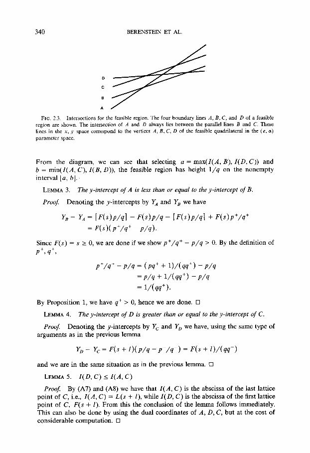
FIG. 2.3. Intersections for the feasible region. The four boundary lines A, B, C, and D of a feasible region are shown. The intersection of A and D always lies between the parallel lines B and C. These lines in the x, y space correspond to the vertices A, B, C, D of the feasible quadrilateral in the (e, a) parameter space.

From the diagram, we can see that selecting a = max(I(A, B), I(D, C)) and b = min(I(A, C), I(B, D)), the feasible region has height 1/q on the nonempty interval [a, b]..

LEMMA 3. The y-intercept of A is less than or equal to the y-intercept of B.

Proof. Denoting the y-intercepts by YA and YB we have

Y ~ - YA = [F(s )p /q] - F ( s ) p / q - [ F ( s ) p / q l + F ( s ) p + / q +

= F ( s ) ( p + / q + - p / q ) .

Since F(s) = s > O, we are done if we show p+/q+ - p / q > 0. By the definition of p+,q+,

p+/q+ - p / q = (pq+ + 1) / (qq +) - p / q

= p / q + 1 / ( q q +) - p / q

= 1 / ( q q + ) .

By Proposition 1, we have q+ > 0, hence we are done. []

LEMMA 4. The y-intercept of D is greater than or equal to the y-intercept of C.

Proof Denoting the y-intercepts by Yc and Yo we have, using the same type of arguments as in the previous lemma

Yo - Yc = r ( s + l ) ( p / q - p - / q - ) = r ( s + l ) / ( q q - )

and we are in the same situation as in the previous lemma. []

LEMMA 5. I (D, C) < I(A, C)

Proof By (A7) and (A8) we have that I (A, C) is the abscissa of the last lattice point of C, i.e., I (A, C) = L(s + l), while I(D, C) is the abscissa of the first lattice point of C, F(s + l). From this the conclusion of the lemma follows immediately. This can also be done by using the dual coordinates of A, D, C, but at the cost of considerable computation. []

SUBPIXEL REGISTRATION A C C U R A C Y 341

The same proof yields

LEMMA 6. I (A, B) <_ I(D, B).

From what we have just said, it follows that

0 < a = max( I (A , B), I (D , C)) < m i n ( I ( A , C), I (B , D))

= b E N ,

hence we are guaranteed that there exists an x ~ [0, N] such that the feasible region over x has height 1/q. Therefore, if we pick the fine L 0 which is the average of B and C (i.e., for each x, average the corresponding y-coordinates of B and C), we have

min max I L ( x ) - L0 (x ) [ < 1 / ( 2 q ) , (11) O<x<~N L ~ ( N , q , p , s )

where L(x) , Lo(x ) represent the ordinate of the points in L and L0, with abscissa X.

The meaning of (11) is that given a digital fine with period q in the sensed image and such that the underlying real edge has slope between zero and one, then we can determine the vertical offset between sensed and reference images to an accuracy of 1 /2q pixels. Thus we can define a vertical translation between the reference and sensed images, such that the y-coordinate of any translated point differs by no more than 1/2q from the correct y-coordinate.

We remind the reader that in the introduction we have discussed how this estimate could be used to obtain estimates for the offsets Ax, Ay between the sensed and the reference images.

4. INFINITE DIGITAL LINES

The feasible region for infinite digital lines is easily computed using the results of Section 3. This analysis is divided into two parts. For any infinite digital line of period q, we show the channel consists of two parallel fines, which are a vertical distance 1/q apart. Thus, since the channel extends over the whole x-axis, there is no flaring at the end as in the finite case. If the infinite digital line is aperiodic, then we show the channel extends over the whole x-axis, but consists of a single line. Thus the maximum error is 1/2q of the digital line if the digital line has period q and zero if the digital line is aperiodic. The aperiodic infinite digital fines are precisely those infinite digital fines which are the digitizations of fines with irrational slope. Since the irrationals are a set of measure one in the unit interval, using the uniform probability measure, we see that the error is zero with probability one for infinite digital lines.

Before considering the periodic and aperiodic lines separately, we note that any two infinite lines with the same digitization are parallel. Let y = mx + b and y = nx + c be two fines. Then the difference, h(x), in the y values of these fines at x is given by h(x) = (m - n)x + (b - c). If m and n are not equal then there exists a K > 0 such that Ih(x)l > 1 for all x such that Ixl > K. Thus the two lines cannot have the same digitization.

We now consider the case of infinite digital fines of period q. By the feasible region description in Section 2, the lines corresponding to the vertices, A, B, C, and

342 BERENSTEIN ET AL,

D of the feasible region in (e, a) space have slopes p - / q - , p / q , p+/q+. Fixing p, q, and s and letting N go to infinite, we see the above result on the slopes of infinite lines having same digitization imply p - / q - , and p+/q+ must approach p / q . Inserting these limits into the formulas for the vertices A and D, we see that, in the limit A = B and C = D. We have shown in Section 3 that B and C are a vertical distance 1 / q apart. This establishes the result for the infinite periodic digital line.

The infinite aperiodic line requires a different approach. We first cite a version of a classical result [4] on lines with irrational slope. Let f ( x ) = mx + b be a line with m irrational. Then the set { m x + b - [mx + bl: x is an integer} is dense in the unit interval. It has already been shown that two lines with the same digitization have the same slopes and can only vary in their y-intercepts. Let e > 0 be given. Then the digitization, L, of the line y = m x + b (m irrational) is aperiodic so there exists integers K 1 and K 2 such that m K I + b - [mK 1 + b] < e and rnK 2 + b - [mK 2 + b] > 1 - e. Thus decreasing b by more than e would change the digitization at K 1 and increasing b by more than e would change the digitization at K 2. Thus for any

> 0, we cannot change b by more than e without changing the digitization. Hence b is fixed. Since m is also fixed, the channel is the single line y = m x + b.

5. INVARIANT LINE MEASURE

A probabilistic analysis of geometric accuracy requires a probability distribution in the fundamental objects, the lines. It is tempting to place a uniform distribution on the coefficients of the lines represented in some parametric form. Unfortunately, there is no canonical parameterization and the measure will not be uniform with respect to other parameterizations. A customary escape from this quandary is to impose some parameterization independent conditions which single out a probability measure. In geometric probability problems, one generally assumes the measure is invariant under translation and rotation of the geometric figures, in our case the lines. This uniquely determines a coordinate system, the (p , if) polar coordinates of a line, in which the distribution is uniform with respect to the parameters as shown in [9, p. 28]. To write this measure in terms of the dual coordinates we appeal to Fig. 5.1.

We clearly have

p = e . cos(@ - ~r/2) and ~r/2 - 0 = ~r -

J

, ~ , ~ 0 y=O'x +e

FIG. 52. Coordinate system for line parameters.


hence

and

p = e �9 cos 0

dp dep = (cos 0 d e - e sin O dO ) A dO = cos O de dO.

Using tan 0 = a we obtain dO = cos20 da = (1 + a2) -1 da, so finally

dpdq~ = (1 + a2)-3/2deda (12)

is the invariant measure. We want to normalize (12) so that total measure of 0 < e < l , 0 < a < l i s e x a c t l y l . From

f ( 1 + a2)-3/2da = a(1 + 0/2)-1/2 (13)

f0/(1 + 0 /2) -3 /260 /= - ( 1 + 0/2) 1/2 (14)

we obtain that the normalized invariant measure is

a/, = v~-(1 + 0/2) -3/2 dedm (15)

It is now easy to compute faf(e, 0/)d~, where fl is the quadrilateral A, B, C, D formed by the lines of code (N, q, p, s). It is just necessary to recall the Eq. (A9) and (A10) of the sides of this quadrilateral:

p + / q + Wl - a z 1 Sfd/~ : ~/2 { ;/q (f~o_.Xo f(e, 0/) de) (d0//(1 + 0/2)3/2)

plq Yl - axt e + fp /q (fwo azof( ,0/)de)(d0//(l+0/2)3/2)}. (16)

In particular, using the definitions of p+, q+, p , q which appear after (A10):

"(") = ~I fn+/q+(( W1 --Yo) q- 0/(Xo- Zl))(d0/l(1 q- 0/2) 3/2 ) tWp /q

p/q + s , - Wo)+ 0/(z o -x,))(da/(l + 0/2)3/2)I =~(fpO+/q+(p+_q+0/)(d0//(i/q +0/2)3/2)

p/q + s (-p +0/q-)(d0//(l + 0/2)V2)}

= V~-{1/((p+)2 + ( q + ) 2 ) 1 / 2 (pp+ + qq+)/(p2 + q2)l/2

)' + l / ( ( p + ( q - ) 2 ) l / 2 - ( p p - + q q - ) / ( p 2 + q 2 ) X / 2 } .


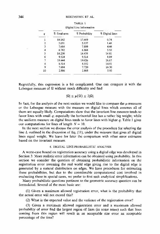
TABLE 1

Digital Line Information

q % Total area % Probability % Digital lines

1 18.182 17.469 0.74 2 5.051 5.137 1.48 3 7.684 7.809 4.44 4 6.782 6.868 5.93 5 14.250 14.438 14.81 6 9.524 9.514 8.89 7 19.444 19.626 26.67 8 8.514 8.552 14.81 9 7.684 7.720 16.30

10 2.886 2.868 5.93

Regretfully, this expression is a bit complicated. One can compare it with the Lebesgue measure of ~ without much difficulty and find

lal-< tL(a) _< 21f~l.

In fact, for the analysis of the next section we would like to compare the/~-measures or the Lebesgue measure with the measure on digital lines which assumes all of them are equally likely. Computations show that the invariant line measure tends to favor lines with small q; especially the horizontal line has a rather big weight; while the uniform measure on digital lines tends to favor lines with higher q. Table 1 gives our computations for lines of length N = 10.

In the next section we discuss the error analysis of the procedure for selecting the line L outlined in the discussion of Eq. (11), under the measure that gives all digital lines equal weight. We leave for later the comparison with other error estimates based on the invariant measure.

6. DIGITAL LINE-PROBABILISTIC ANALYSIS

A worst-case bound on registration accuracy using a digital edge was developed in Section 3. More realistic error information can be obtained using probability. In this section we consider the question of obtaining probabilistic information on the registration error assuming the real world edge giving rise to the digital edge is generated by a natural distribution on edges. We have procedures for estimating these probabilities, but due to the considerable computational cost involved in evaluating these in special cases, we prefer to first seek analytical simplifications.

Many probabilistic questions pertinent to the geometric accuracy question can be formulated. Several of the most basic are:

(1) Given a maximum allowed registration error, what is the probability that the actual error will not exceed this?

(2) What is the expected value and the variance of the registration error?

(3) Given a maximum allowed registration error and a maximum allowed probability of error find the largest region of lines (in some sense) such that lines coming from this region will result in an acceptable size error an acceptable percentage of the time?


We now turn to an analysis of the first question. We wish to determine, for any acceptable error level in the estimated offset between sensed and reference image, what is the probability that a random edge will result in a digitization which permits estimation to less than that error level. Though a simple formula for these probabilities as a function of digital line length is not available, a procedure for calculating these probabilities for any given line length, N, is described and results for the case N = 10 are presented. In addition we present asymptotic upper bounds on the error.

The basic approach to computing the error probabilities is quite simple. A probabili ty density function is given on the set, A, of all lines with slope between 0 and 1, going through the pixel with lower left vertex (0, 0). Since a line has only one chain code, the sets of lines with different chain codes gives a partition of the set A. Hence the density on lines induces a density on chain codes. For a chain code with period q, the maximum error is 1/2q as was shown in Section 3. Thus for any specified error h, we must calculate the probability of the following set, B, of line chain codes:

B = ( (N , q, p, s) : 1/2q < h ) .

The set of all linear chain codes of length N can be enumerated. For each chain code in B, the corresponding feasible quadrilateral can be calculated as in Section 2. The density function on lines can then be integrated over the quadrilateral and the sum of these integrals over all members in B computed. This sum yields the desired probability.

The problem of enumerating linear chain codes of lines through the origin was discussed in [8] where also an algorithm for generating the set of linear chain codes was presented. We have not found any estimates in the literature of the number of chain codes of a given length. The problem is that the shortest period of the digital line of length N corresponding to a line

y = ( p / q ) x + m / q

might be strictly smaller than q. Since lines and we can associate to each a characterizing those values of s for (N, fi, ~r g) with ~ < q. The answer lies

such lines generate all the possible digital code (N, q, p, s), the problem reduces to which this code does not coincide with in the following.

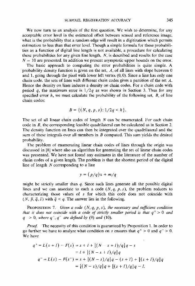
PROPOSITION 7. Given a code (N, q, p, s), the necessary and sufficient condition that it does not coincide with a code of strictly smaller period is that q+ > 0 and q- > O, where q+, q- are defined by (9) and (10).

Proof The necessity of this condition is guaranteed by Proposition 1. In order to go further we have to analyze what condition on s ensures that q § > 0 and q - > 0. We have

q + = L ( s + l) - F(s ) = s + l + l ( N - s + l ) / q ] q - s

= l + l ( N - s + l ) / q ] q

q - = L ( s ) - F(s +) = s + [ ( N - s ) / q ] q - (s + l) + [ ( s + l ) / q ] q

= [ ( N - s ) / q ] q + t ( s + l ) / q ] q - l.


Note that if N - s > q then we have that the digital line has period q, since the digits in the chain code corresponding to x = s + 1 , . . . , x = s + q < N, form the chain code of the standard line, i.e., of y = ( p / q ) x . Of course in this case we also have N - s - l _ > q - l > 0 h e n c e q + > l > 0 and q - _ _ _ q , l > 0 . Suppose now N - s < q; then the condition q - > 0 implies that s + I > q and hence we have F ( s + l) = s + l - q. Note that

N - F ( s + I) = N - ( s + l ) + q > q,

since q+ > 0 implies that N - (s + l) > 0. So we only have to prove that a line for which N - s < q, and N - F( s + l) > q has smallest period q. Notice that this says that the line y = ( p / q ) x + m / q passes through a single lattice point at x = s, while the line y = ( p / q ) x + (m + 1 ) / q contains two lattice points, the first one with abscissa F ( s + l) < s. We know hence that this second line has period exactly q, since if we restrict ourselves to F ( s + l) + 1 < x < F ( s + l) + q < N the q digits in the chain code of the second line are those of the standard chain code. To prove that the original line has smallest period q it is enough to show that the same port ion of its chain code has smallest period q since the period of a chain cannot be smaller than that of any subchain. That is, we have reduced ourselves to show that the chain code of the digital line of length q corresponding to y = ( p / q ) x + (q - 1 ) / q has smallest period q. Calling c i the standard chain code and c* the chain code of this other line, it would be enough to prove that the sequence { c{' . . . . ,c~ } is exactly the sequence { Cq, . . . , c 1 ) making an appeal to (1). Now, as we have argued in Lemma A1, the code { c1" . . . . , c~' } is obtained from ( c l , . . . , Cq }

* = 0 , c 7 = c j , 1 < j < q - 1, while c 1 = 0 , Cq= 1. Tof in ish by making cp' = 1, Cq the proof we only need to show that the sequence c 2 . . . . , %-1 is symmetric, i.e.,

Cj -~" Cq_j+ 1.

But cj = [(p/q)j] -[(p/q)(j- 1)] a n d

Cq_j+l = [ ( p / q ) ( q - j - 1)] - [ ( p / q ) ( q - j ) ]

= p + [ - ( p / q ) ( j - 1)J - ( p + [ - ( p / q ) j ] ) .

As long as x is not an integer we have [ - x ] = - I x ] - 1. But 2 < j < q - 1 indicates that neither ( p / q ) ( j - 1) nor ( p / q ) j are integers, hence

Cq_j+ 1 = - - [ ( p / q ) ( j - 1)] - 1 - ( [ ( P / q ) J ] - 1) = cj.

Due to the above characterization of c* we have

c 7 = Cq_j+ 1, 1 <_j < q,

which shows that the digital line of length N corresponding to y = ( p / q ) x + (q - 1 ) / q has smallest period q, and hence the same is true for the original line. []

Proposition 7 and its proof gives us a way to compute the number L ( N , q) of digital lines of length N and smallest period q. In fact L ( N , 1) = 1, so we can consider q > 1, then the situation N - s < q can only arise if N _< q + s - 1 _<


2q - 2, that is, ( N + 2) /2 < q. Hence, if q < ( N + 2)/2, s can take arbitrary values and it follows that

L ( N , q ) =qep(q) for 2 < q < ( N + 2 ) / 2 , (17)

where q,(q) is the Euler function that counts the number of values p, 1 < p < q, p A q = 1. This formula is clearly valid for q = 1 since q~(1) = 1. In the remaining range of q we can use that when p runs over all the values considered in q,(q), so does l, where we remind the reader l is defined by (4). We fix I and divide the range of s into two classes

O < s < N - q , N - q + l < s < q - 1 .

The second class is not empty since we are assuming N + 2 < 2q. In the first class every line has smallest period q, this accounts for N - q + 1 lines. In the second class we have two subclasses, s + l < q and q < s + l . The first one cannot introduce any lines of period q due to the condition q - > 0. In the second one we have to consider whether

N - ( s + l - q ) ~ q

or not. Only if this inequality is true do we get new lines (due to the condition q+ > 0). Hence we must have

m a x { q - l , N - q + l ) < s < m i n { q - l , N - l }

which gives u s l + min{l - 1, N - q, 2q - N - 2, q - l - 1} lines (notice that this min imum is nonnegative). Therefore, in this range of values of q we have

L ( N , q ) = ( N - q + 2)q~(q) + E m i n { 2 q - N - 2 , q - l - l , l - l , N - q } , 1

(18)

where the sum takes place over all values l, 1 < l < q - 1, l A q = 1. Since this expression is a little bit hard to work with, we can use upper and lower estimates, L**(N, q ) = qq,(q), L . ( N , q ) = ( N - q + 2)q~(q) for q in this range. Finally, setting L ( N ) = total number of digital lines of length N, we get the estimates

IN/2] N

L . ( N ) = ~_, qqJ(q) + ~ ( N - q + 2)q,(q) q = l (N/2)+ l=q

N

< L ( N ) < L * * ( N ) = Y'~ qeo(q). (19) q = l

Using the above formulas we can produce Table 2 for N = 10. We notice that L ( N ) is fairly close to L . ( N ) and very different from L**(N) .

L * * ( N ) would have been the count if no digital fines drop their period when considered to have finite length. Since we want to develop some asymptotic bounds


TABLE 2

q ok(q) L,(N, q) L(N, q) L**(N, q)

1 1 1 1 1 2 1 2 2 2 3 2 6 6 6 4 2 8 8 8 5 4 20 20 20 6 2 12 12 12 7 6 30 36 42 8 4 16 20 32 9 6 18 22 54

10 4 8 8 40

Total 121 135 217

for the error of the choice (11) for subpixel accuracy, we introduce a different upper bound function L*(N, q) defined as

L*(N, q) = L(N, q), 1 < q < [ (N /2 ) ]

L*(N, q) = L , (N, q) + (2q - N - 2)(q~(q) - 2),

( N / 2 ) + 1 < q < ( 2 ) N +

L*(N,q) = L , (U,q) + ( N - q)(q~(q) - 2), ( ~ ) U + ~ < q < N . (20)

The choice is motivated by choosing the smallest of the two terms independent of l in the minimum that appears in (18). Since the values l = 1, l = q - 1 make this minimum zero we only have ( q f f q ) - 2) terms in the sum. We also note that L*(N, q) = L,(N, q) for q = ( N / 2 ) + 1 (if this value is an integer) and for q = N. For N = 10, we have only three values to compute

L*(N, 7) = 38, L*(N, 8) = 20, L*(N, 9) = 22

which gives L*(10) = 137 in this case, a very good approximation! (We have used L*(N) N * = E q = l t (N , q).)

PROPOSITION 8. The exact number of digital lines is given by the formula L( N) = Eq=IL(N, q), L(N, q) defined by (17) and (18). It satisfies the inequalities

L , (N) < L (N) < L*(N),

where the functions L,( N), L*( N) have been defined above and satisfy the asymptotic estimates

L , ( N ) = (3/4~rZ)N 3 + O(N21ogN) = 0.076N 3 (21)

L*(N) = (10/9TrZ)N 3 + O(N21ogN) = 0.112N 3. (22)

We only have to prove the estimates (21) and (22). We use the methods

N

O(N) = Eep(q) = 3N2/~r 3 + O(N log N ) . (23) 1

Proof used in [4] to prove the asymptotic formula


The idea is to write do using the Moebius function/~

do(q) = q E i x ( d ) / d . alq

It will be useful to find first the asymptotics of L**(N). For any N,

N N

L**(N) = ~_~ qdo(q) = ~_, q2]~_~(d)/d. q = l q = l dlq

(24)

We now write q = dd' and substitute in the last term:

L * * ( N ) = • d2(d')21~(d)/d dd" <_N

N

= E dlx(d) E (d') 2" �9 d = l d '<_N/d

The term ~,a'<_ N/d(d') 2 = (1/3)(N/d) 3 + O(N2/d2) �9 Inserting this in L**(N), we obtain

N

L**(N) = (1/3)N 3 Z IL(d)/d2 + O(NZlogN)- d = l

Note we have used

a=@ a~(d)N2/d2 u < N 2 Y'~ 1 / d = O(NZlogN). d = l

But we have 2~#(d ) /d 2 = 6 /~ 2 [4]. Hence, 2~tz(d)/d 2 = 6/~r 2 + O(1/N). Sub- stituting this into L**(N), we get

L**(N) = 2N3/rr 2 + O(N21og N). (25)

We can now get the asymptotic formula for L,(N). Recall that we have, from (19),

L , ( N ) = U3/(47r 2) + O(NZlog N)

N N

+ ( N + 2 ) ~ do(q)- ~ qdo(q). ( N / 2 ) + 1 ( N / 2 ) + 1

We can write

N

do(q) = * ( N ) - 0 ( N / 2 ) ( N / Z ) + 1

= 3N2/rr 2 - 3N2/4~r 2 + O(N log N)

= 9N2/(4~r 2) + O(N log N).


Similarly

N

E (N/2) + 1

q,~(q) = L** (N) - L** (N / 2 )

= 2N3/rr 2 - (2 / r r2 ) (N/2) 3 + O(N21og N)

= 7N3/(47r 2) + O ( N Z l o g N ) .

So that we finally get L , ( N ) = 3N3/(47r 2) + O(N21og N). Using the definition (20) we obtain

(2/3) N + 2/3 (2/3) N + 2/3

L * ( N ) = ~_~ qq~(q) - 2 E (2q - N - 2) 1 (N/2 )+ 1

N N

+(2N + 2) • ~b(q)- 2 E qep(q) (2/3) N + 2/3" (2/3) N + 2/3

N

- 2 Y'~ ( N - q ) (2/3) N + 2/3

= L**( (2 /3 )N + 2/3) + 2 N ( ~ ( N ) - ~ ( (2 /3 )N + 2/3))

- 2 ( L * * ( N ) - L * * ( ( 2 / 3 ) N + 2/3)) + O(U2).

We introduce now (23) and (24) into this expression:

L * ( N ) = (6 /~rz ) ( (2 /3 )N) 3 - 4 N 3 / ~ r 2 + 6N3/~r 2

- (6N/~r2) ( (2 /3 )N) 2 + O(N21og N)

= (10/(9~r2))N 3 + O(N21ogU) .

We note that L , ( N ) = 0.076N 3 and L * ( N ) = 0.112N 3 if we disregard the O(N21og N) term; for N = 10 these approximations are not very good. Neverthe- less for the coming estimates it is only the leading term that counts. []

Remark. On purely heuristic grounds one can propose an approximate formula L ( N ) to the correct value L ( N ) . It consists in assuming that the values l that appear in (28) are uniformly distributed with density ep(q)/q. Then

Z ( U ) = +

N

+ E

(2 /3) N + 2/3 2~ (q~(q) /q)(2q - N - 2)(N - q)

(N / 2 )+ 1

( e p ( q ) / q ) ( N - q)(2q - N). (2 N / 3 ) + 1

It is clear that L . ( N ) _< L(N) and also L ( N ) < L*(N) , since N - q < q and 2 q - N < q in both sums. It is not apparent how to find the correct relation between L ( N ) and L(N) but we note that for N = 10 from Table 2 we im-


mediately get the remarkable value

L(10) = 135.47.

Besides, one can show, by the same methods used in Proposition 8, that the following asymptotic development holds

[,(N) = N3/cr 2 + O(NZlog N)

which fits right between the values in Proposition 8. It is tempting to conjecture that L ( N ) has the same asymptotic behavior. In fact, we computed L(N), using (17) and (18), and L (N) for N = 100 and found the following values

L ( N ) = 104,359

/~ (N) = 104,949

L ( N ) / N 3 = 0.104359

1/~r 2 = 0.101321

which clearly reinforces the conjecture.

Let S(N) be given by

N

S(N) = ~ ( 1 / q ) L ( N , q ) . (26) q = l

Then the offset error incurred by using the line parallel to B passing through the middle of the channel is given by

E(N) = ( ( 1 / 2 ) S ( N ) ) / L ( N ) (27)

when we use the uniform distribution on digital lines.

PROPOSITION 9. Up to terms of the form O((log N ) / N 2) the offset error defined in (27) satisfies the estimates

59 ( ~ ) ( 1 / N ) < E ( N ) < ( ~ ) ( 1 / N ) . (28)

Proof We start with the lower bound for E(N). It is clear that E(N) > 1/(2N). To improve on this we note that up to q = N/2 the sum of the terms in S(N) is exactly ap(N/2), hence

N

(I)(N/2) + ~ (1 /q )L (N , q) ( N / 2 ) + 1

2 E ( N ) = L**(N/2) + ( L ( N ) - L**(N/2))

1 NCg(N/2) + ( L ( N ) - L**(N/2))

N L**(N/2) + ( L ( N ) - L**(N/2))"


Now Nc~(N/2) > L**(N/2) because in S(N) we divide by q, and here we are considering 1 < q < N/2 only. It is easy to see that the function (a + x) / (b + x) is strictly decreasing if a > b, hence the above expression diminishes if we replace L(N) by L*(N) and we obtain

2 E ( N ) > 1 Nd~(N/2) + (L*(N) - L**(N/2))

N L**(N/2) + (L*(N) - L**(N/2))

(I)(N/2) + (L*(N) - L * * ( N / 2 ) ) / N

L*(N)

(3/~r2)(N2/4) + (((lO/9)N3)/Tr 2 - (2/~rZ)(N3/8))/N

( (10/9) N3 ) /~r 2

+ O(log N / N 2)

= (2~)(1/N) + O(logN/N2).

Therefore we get

29 O(log N / N 2). E (N) > (ag)(1 /N) +

Let us now work an upper bound for E(N). We use a slightly more complicated method. Replacing L(N, q) by L*(N, q) in the expression of S(N) we have

S*(N) = (2/3) N+ 2/3 N

q~(q) - 2 ~ q~(q) 1 (2/3) N + 2/3

N

+ 2 N E (eo(q)/q) + O(N). (2/3) N + 2/3

The only new difficulty consists in estimating the term E(eo(q)/q). Using the formula (24) we get

N

E (eo(q)/q) = E E ~ ( d ) / d (2 /3 )N+2/3 q dlq

N

= ~, ( t*(d) /d) ( (1 /3) (N/d) + O(1/d)), d = l

since by writing q = d d ' , we get ((2)N + 2)/d < d' < N/d. By the same argument we used to obtain (25) we see that this term is exactly

(N/3)(6/~r 2) + 0(1) .

The first two terms in S*(N) can be computed using (23), and we finally get

S*(N) = 2NZ/~r 2 + O(N).


On the other hand,

S(N) + (L*(N) - L ( N ) ) / N < S*(N).

Dividing by L*(N) we obtain (up to O(log N/N2))

( L ( N ) / L * ( N ) ) ( ( S ( N ) / L ( N ) ) - 1/U) + (1/N)(ag/lO)(1/N).

But L(N) /L*(N) >_ L.(N)/L*(N) -- ~6,27 hence 2 E ( N ) - 1/U _< ( ~ ) ( ~ ) ( 1 / N ) which leads to the estimate (28). []

Remark. Corresponding to the heuristic estimate L ( N ) given above for the correct number of lines L(N) we can construct a heuristic formula for the asymptotic error, /~(N),

ff~(U) = (1 /2 ) (S (N) /L(N) ) ,

N / 2 N

S ( N ) = ~ q~(q) + Y'~ q~(q)((4U + 2 ) / q - 3 - (N2/q2)). 1 N / 2 + 1

where

One finds, using the same type of reasoning as in Proposition 9,

S ( N ) = (6(1 - l og2)N2) / I r 2 + O(N log N )

/~(N) = (3(1 - l o g 2 ) ) / ~ r 2 ( 1 / N ) + O(logN/N 2)

- 0 .92/N,

TABLE 3

Error Probabilities for Digital Lines without Points Missing

Error Probability (max error) > Error

0.5000 0.0000 0.2500 0.0147 0.1666 0.0294 0.1250 0.0735 0.1000 0.1323 0.0833 0.2794 0.0714 0.3676 0.0625 0.6323 0.0555 0.7794 0.5000 0.9412 0.0000 1.0000

Note. Given an entry, a, in the first column, the corresponding entry in the second column is the percentage of digital lines of length ten whose maximum registration error exceeds a. Line length = 10.


which is, in fact, in tune with the upper and lower bounds obtained in Proposition 9, namely 0.72/N and 1.09/N, respectively. It would be very interesting to show that E ( N ) has the same asymptotic behavior as/~(N).

We remark that though the asymptotic behavior of the expected value of the offset with respect to the invariant measure /~ is very hard to obtain due to the nature of the formulas from Section 5, for any concrete value of N it is perfectly possible to compute this expected value using the explicit nature of the formulas for the measure ~(fl) of the quadrilateral associated to any digital line. We have done this for N = 10 and obtained the error probabilities given in Table 3.

CONCLUSIONS

This paper is concerned with the accuracy of registration based on line matching given that the correct digital line is detected, i.e., there are no missing or extraneous pixels. An expected error of approximately 0.1 pixels in the estimation of the vertical offset of a line was derived. In this approach, a straight edge in a scene is represented as a digital line in a sensed image and a real line whose digitization is this digital line is selected. The real line is then matched to the corresponding line in the reference image. Since this paper was written, we have conducted simulation studies [1] on the accuracy of this approach. The approach was also extended to the case where not all pixels in the digitization were correct. In addition, those extensions made use of grey scale information. In that work, the average error in the vertical offset estimation was about 2~ of a pixel for digital lines of length ten. This approach to subpixel accuracy appears promising for problems in both image reigstration and high accuracy edge detection. Extensions of this approach to curved edges is a natural direction for further work.

In the process of obtaining the error estimates for edge accuracy determination, we have obtained an exact formula for the number of digital lines of a given length. Up to now, only the count of the number of digital lines which are digitizations of real lines through the origin have been computed. A natural question that arises in this context is the counting of various other digital geometric objects. Since the formula counting all digital lines is complicated, we give heuristic reasons that support the conjecture that the asymptotic behavior of this number of lines is N3/rr 2. For N = 100, the exact formula and the conjectured asymptotic behavior differ only by 0.5%. We consider the problem of proving this conjecture an interesting mathematical problem.

APPENDIX A

Here we provide the proofs of the formulas (4)-(10) of Section 2. An alternate proof appears in [2].

We begin with an observation from [10] which remains valid for lines of finite length N due to the fact that all digital lines arise out of the digitization of lines of the form y = p / q x + m / q , 0 < m < q , p A q = l (we assume q > 1 since for q = 1 we only consider the line y = 0).

LI~MMA A1. For a line of slope p /q , vertical displacement upwards by 1 /q units results in a cyclic shift of the code by I digits to the right within each segment of length q, where I is the solution of the equation

lp -- - l ( m o d q), 0 < l < q. (A1)


Proof. For the purpose of this lemma we can consider a digital line of infinite length generated by the line of equation y = ( p / q ) x + e, 0 < e < 1. When e = 0 the line contains exactly those points in the lattice Z 2 of the form (kq, kp), k ~ Z.

When e is increased the code remains the same until new lattice points lie on the line; if a new lattice pont (q' , p ' ) appears for a value eo, then one gets a transposition of the 0 which corresponds to x = q' and a transposition of the 1 that corresponds to x = q ' + 1 for values of e < e 0, e ~ e0, as a quick look at the picture shows. The points ( q ' + kq, p ' + kp), k ~ Z, belong to the line y = ( p / q ) x + e o and no other lattice point does, otherwise the slope could not be p / q

with p / x q = 1. Notice that because of the upward shift we have 0 < q ' < q and 0 < p ' < p for the first value e 0 where the above transposition takes place. This implies that the code of the line y = ( p / q ) x + e o is the same as that of the line y = ( p / q ) x with a right cyclic shift in each period of size q'. The same fact will hold between any two successive upward shifts of the same magnitude e. It remains to identify this magnitude e 0 and the value q'. Since e o is the first positive value for which such a shift recurs, we have that the parallelogram of vertices (0, 0), (q, p) , (q ' , p ') , and (q + q', p + p ' ) is a minimal parallelogram on the lattice (see [4, p. 28]) and hence its area is exactly one, i.e.,

p'q - q'p = qe o = 1. (A2)

F rom this it follows that e 0 = 1 / q and q' is the quantity defined as l by (A1). After successive transitions of this size (or what is the same, after q successive cyclic shifts of s ize / ) , we go back to the original code. []

We are now ready to relate the code (N, q, p, s) to the family of lines that induce the same code. First, we know that it is induced by a line of the form

y = ( p / q ) x + m / q 0 <_ m < q (A3)

and we would like to find the relation between s and m. Lemma A1 tells us that

Hence, we have

lm =- s (mod q) . (A4)

s = lm - kq for some k > 0; (A5)

in fact, using the function F introduced in (2) we can write

s = F ( l m ) ,

since all the function F does is select a representative in 0 , 1 , . . . , q - 1 for every element in Z / q Z . Substituting the expression (A5) into (A3) we obtain

y = ( p / q ) s + m / q = (ptm)/q + m / q - kp = p ' m - kp ~ Z, (A6)

where the third identity was obtained using (A2) (Recall / = q ' in (A2).) That is, we see that the value s has the property that for x = s the point in the line (A3) is a lattice point. Furthermore, this is the first lattice point in the interval 0 < x < oo


which lies on the line. Otherwise the slope of the line will be rational with a denominator strictly smaller than q and in contradiction to the fact that we are assuming that the chain code has smallest period q (this justifies the letter F to denote the function on 7 / q Z as defined by (2)). We can also conclude that the value y in (A6) is given by

y = [ ( p / q ) s ] and m / q = [ ( p / q ) s ] - ( p / q ) s ,

since 0 < m / q < 1. This tells us that the line (A3) coincides with the line B given by the dual coordinates (6), i.e.,

e = [ F ( s ) ( p / q ) l - F ( s ) ( p / q ) , a = p / q .

As a corollary of this representation and Lemma A1 we obtain that the line

y = ( p / q ) x + ( m + 1 ) / q

coincides with the line C described by (7), namely the infinite line will have first lattice point when x = F(s + l). Since 0 < (m + 1 ) / q < 1, we have for the corresponding value of y that

y = [ F ( s + l ) ( p / q ) l + 1.

Hence it follows that he dual coordinates of C are, in fact,

e = 1 + [ F ( s + l ) ( p / q ) l - F ( s + l ) ( p / q ) , a = p / q .

We could, by abuse of language, denote the chain code of C as (N, q, p , F ( s + l)), but it might not be the case that q is the smallest period of this code, as we have in the example:

so that l = 7 and

which has code

B ~ (11 ,11 ,3 ,0) o y = (3 /1 1 )x

C o (11,11,3 ,7) o y = ( 3 / l l ) x + 1/11

0001 001 0001

whose smallest period is 7. Let us call "last lattice point of a line" the one with the largest abscissa still _< N.

We are going to consider now two other lines defined by:

A is the line passing through the first lattice point of the line B and the last lattice point of the line C. (A7)

D is the line through the first lattice point of C and the last lattice point of B. (A8)


Those two lines are well defined and not vertical since no point of B coincides with a point of C and these lattice points cannot be above each other. Neither of these two lines nor the line C have code (N, q, p, s) since they pass through lattice points different than those corresponding to B. Let us first derive an important property of this collection of four lines A, B, C, D. We note that if we have two points in the dual space L 1 = ( e l , Otl) , L 2 = ( e 2 , 0 t 2 ) which correspond to lines with code (N, q, p, s) then the point L of coordinates

e = ) ~ e 1 + ( 1 - X ) e 2 , a = X a 1 + ( 1 - ) ~ ) a 2 , 0 < X < 1,

corresponds to a line which passes through the same pixels as L1 and L2; in fact for a given x, the ordinate y of the corresponding point in the line L is just Y = ~Yl + (1 - k)Y2, with (x, Yl) ~ L1, (x, Y2) ~ L2- So the set of lines with code (N, q, p, s) forms a convex set in the dual space. Furthermore, it is easy to see that this convex set f~ must contain an open neighborhood of the open segment defined by B and C. This is simply the fact that a line between B and C passes through the same pixels as B but passes through no lattice points (by Lemma A1) hence its slope can be jiggled a bit and keep the same code.

We are going to look at the (possibly degenerate) quadrilateral with vertices A, B, C, D. For that purpose we need to find the equations of the sides, e.g., the side A B . We are looking for the equation of a line in the dual space, that is, an equation of the form

a a + be = c, a 2 + b 2 4= O.

The definition of A shows that A and B have a point in common, namely the first lattice point of the line B, say (x0, Y0), and hence every line which corresponds to a point in A B passes through the same point, i.e., it satisfies the equation

Xoa + e =Y0

which has the desired form. Calling (z0, w0) the last lattice point of B, (X1, Yx) the first lattice point of C, (z 1, wl) the last lattice point of C we have the equations

A B : xoa + e =Y0

B D : zoa + e = w o

D C : XlOL Jr e = Yl

C A : z l a + e = w 1.

(A9)

We note that on one side of the line A B we have xoa + e > Y0 and on the other side we have Xoa + e < Yo. On this second side we have that no line passes through the same pixels as B, hence it cannot have code (N, q, p, s), therefore f~ _c ((e, a): x o a + e > Y0 }- We can conclude by a similar reasoning that:

___ {xoa + e >--Yo) n {Zoa + e > Wo) n {XlO/--t- e < Y l ) n {ZlO~ --1- e < Wl}

which is the quadrilateral determined by A, B, C, D. To finish the proof all we need to know is that the half-open segments (A, B] and

[B, D) are in fL For the first one it follows from the fact that there are no lattice


points in the open triangle whose sides are the y-axis, line A and line B. Otherwise we consider the line through such a lattice point (x2, Y2) and ( x o, Yo). It will have the same code as B but clearly has period x o - x z which is strictly less than q (recall Xo = s < q). Similar reasoning holds for the other segment. Summarizing, we have

LEMMA A2. The convex set f~ of all lines coincides with the (possibly degenerate) quadrilateral o f vertices A, B, C, D.

LEMMA A3. I t is never the case that A = D; i.e., it is impossible that we have simultaneously that

(Xo, Yo) = (Zo, Wo) and (xl , Yl) = (7-1, Wl)-

Proof In this case f~ is a triangle (it cannot be a segment since A ~ B C says that A is parallel to B, which contradicts (A7)). One of the sides is BC. Hence fl cannot contain an open neighborhood of the open segment (B, C). This contradicts an observation made above. []

It remains to write down the dual coordinates of A and D. For that we need to consider which is the abscissa of the last lattice point on the lines B or C. For the line B we have that the abscissa of the first lattice point is x = s, hence the last lattice point is x = s + k q , k>__O,x < N . This implies that k = [ ( N - s ) / q ] , hence we get

x = s + [(N - s ) / q ] q = L ( s ) (as defined by (3)).

Since the function L turns out to be a function well defined on Z / q Z , we have that the abscissa of the last lattice point in C is L ( s + l). We get the following formulas companion to (A9)

x o = F ( s )

Zo = L ( s )

X 1 = F ( s + 1)

z 1 = L ( s + l )

Yo = [ ( p / q ) F ( s ) ] = ( p / q ) F ( s ) + m / q

w o = [ ( p / q ) L ( s ) ] = ( p / q ) L ( s ) + m / q

Yl = 1 + [ ( p / q ) F ( s + l ) l = ( p / q ) F ( s + l ) + ( m + 1 ) / q

w~ = 1 + [ ( p / q ) L ( s + l)] = ( p / q ) L ( s + l )

+ ( m + 1 ) / q . (A10)

The line A passes through the points (x 0, Y0) and (zl, wl) hence

a = (w, - y o ) / ( z l - Xo).

Define

q+ = 21 - x 0 , P + = Wl - Yo"

Then

q+ = L ( s + l ) - F ( s )


and

P+ = wl -- Yo = ( P / q ) ( z l -- Zo) -b 1 / q = ( p / q ) q + + 1 / q

verifying (9) and also showing p + / x q+ = 1. We already known that q+ ~ 0; we want to show that Lemma A3 implies q+ > 0. In fact, we have

q + = l + t(N - ( s + l ) ) /q] q

and the only problem that could occur is s + l > N. Then we would have N - s < q and s + l > q which implies that L ( s ) = F ( s ) and F ( s + l) = L ( s + l). This is precisely the situation forbidden by Lemma A3. Now we want to find the ordinate to the origin of A. We have

A: y - Y o = ( p + / q + ) ( x - Xo)

hence, using (A10) we obtain

e = Yo - ( P + / q + ) x o = [ F ( s ) ( p / q ) ] - r ( s ) ( p + / q + ) .

This finishes the verification of (5). Going through the same reasoning for the line D we see that its slope is given by

a = ( p / q ), q - = z o - Xl, P - = W o - y l

so that q - = L ( s ) - F ( s + l) as required and

p - = ( p / q ) z o + m / q - ( ( p / q ) x I + ( m + 1)/q) = ( p / q ) ( z o - x l ) - 1 / q = ( p / q ) q - - 1 / q ,

verifying the relation (10). Writing

D: y - y l = ( p - / q - ) ( x - X l )

and using (A10) again we get

e =Yl + ( P - / q ) x l = 1 + [ ( p / q ) r ( s + l)]

- ( p - / q - ) F ( s + l )

which is the only thing left to check in (8) except for seeing that q - > 0. But this is again Lemma A3. Since q - < 0 only could occur if simultaneously N - s < q and s + l < q, a computation shows this leads to F ( s ) = L ( s ) and F ( s + l) = L ( s + l), which cannot happen.

Summarizing, we have proved

PROPOSITION 1 (SECTION 2). The formulas (2)-(10) defining the quadrilateral A , B, C, D are correct and furthermore q+ > O, q - > O, p+ > O, p - > O.


APPENDIX B: NOTATION

[x] - - g r e a t e s t integer < x

[x] - - l e a s t integer > x

m A n - - g r e a t e s t c o m m o n divisor of m and n

L ( a , b ) - - l i n e jo ining points a and b

~ ( n ) - - E u l e r totient f u n c t i o n - - t h e number of posi t ive integers less than or equal to n which are relatively pr ime to n

/~(n) - - /~ the Moebius funct ion defined as

/~(1) = 1;

if n > 1, let n -- p~ . . . . p~* be the prime decompos i t ion of n. Then

/~(n) = ( - 1 ) k if a 1 = a 2 . . . . . a k = 1

= 0 otherwise.

REFERENCES

1. C. Berenstein, L. Kanal, D. Lavine, E. Olson, and E. Slud, Analysis of subpixel registration, presented at the NASA / Mathematical Pattern Recognition and Image Analysis, Houston, Texas, June 1984.

2. L. Dorst and A. W. M. Smeulders, Discrete representation of straight lines, IEEE Trans. Pattern Anal. Mach. Intell. 6, 1984, 450-462.

3. R. M. Haralick, Digital step edges from zero crossing of second directional derivatives, IEEE Trans. Pattern Anal. Mach. Intell. 6, No. 1, 1984, 58-68.

4. G. H. Hardy and E. M. Wright, An Introduction to the Theory of Numbers, Oxford Univ. Press (Clarendon), London/New York, 1971.

5. P. D. Hyde and L. S. Davis, Subpixel edge estimation, Pattern Recognit. 16, No. 4, 1983, 413-420. 6. E. C. Kim and A. Rosenfeld, Digital straight lines and convexity of digital regions, IEEE Trans.

Pattern Anal. Mach. lntell. PAM1-4, No. 2, 1971, 149-153. 7. D. Lavine, L. N. Kanal, C. A. Berenstein, E. Slud, and C. Herman, Analysis of subpixel registration

accuracy, in Proceedings, NASA Symposium on Mathematical Pattern Recognition and Analysis, Houston, Texas, June 1983, pp. 327-412.

8. J. Rothstein and C. Weiman, Parallel and sequential specification of a context sensitive language for straight lines on grids, Comput. Graphics Image Process. 5, 1976, 106-124.

9. L. A. Santalo, Integral Geometry and Geometric Probability, Addison-Wesley, Reading, MA, 1976. 10. C. Weiman and J. Rothstein, Pattern recognition by retina-like devices, Technical Report OSU-

CISRC-TR-72-8, Department of Computer and Information Science, Ohio State University, 1972.

A geometric approach to subpixel registration accuracy

Documents

Transcript of A geometric approach to subpixel registration accuracy