Ao

TP

a

ARRAA

KEEMNT

1

(tAtsf

efa

•

•

•

•

aT

0d

Electric Power Systems Research 80 (2010) 1160–1170

Contents lists available at ScienceDirect

Electric Power Systems Research

journa l homepage: www.e lsev ier .com/ locate /epsr

generalized model for the calculation of the impedances and admittances ofverhead power lines above stratified earth

heofilos A. Papadopoulos, Grigoris K. Papagiannis ∗, Dimitris P. Labridisower Systems Laboratory, Dept. of Electrical and Computer Engineering, Aristotle University of Thessaloniki, 54124 Thessaloniki, Greece

r t i c l e i n f o

rticle history:eceived 1 September 2008eceived in revised form 10 January 2010ccepted 20 March 2010

a b s t r a c t

A general formulation for the determination of the influence of imperfect earth on overhead transmissionline impedances and admittances is presented in this paper. The resulting model can be used in thesimulation of electromagnetic transients in cases of two-layer earth over a wide frequency range, coveringmost fast transient phenomena of power engineering interest. The propagation characteristics of an

vailable online 24 April 2010

eywords:arth return admittancearth return impedanceulticonductor lines

overhead transmission line over homogeneous and two-layer earth are investigated using the proposedmodel. A systematic comparison of the proposed model with other approaches is also presented and thedifferences due to earth stratification are reported. Finally, the transmission line parameters calculatedby the proposed formulation are used in the simulation of fast transient surges in a transmission lineexcited by double exponential sources.

onhomogeneous earthransient analysis

. Introduction

Overhead transmission line (TL) modelling in electromagneticEM) transient simulations requires the detailed representation ofhe influence of the imperfect earth on the conductor parameters.lthough several approaches have been used since many years,

he accurate modelling of earth conduction effects on transmis-ion lines is still an appealing research topic, especially in the highrequency region for the simulation of fast transients.

Historically, the first approach is the Carson’s homogeneousarth model [1]. Carson proposed the use of earth correction termsor the series impedances, which are derived using the followingssumptions:

The relative permeability of the homogeneous earth is consideredto be equal to unity.The axial displacement currents in the air and in the earth areneglected.

The influence of the imperfect homogeneous earth on the shuntadmittances is neglected.Quasi-TEM (Transverse ElectroMagnetic) field propagation isassumed.

∗ Corresponding author at: Power Systems Laboratory, Department of Electricalnd Computer Engineering, Aristotle University of Thessaloniki, P.O. Box 486, 54124hessaloniki, Greece. Tel.: +30 2310996388; fax: +30 2310996302.

E-mail address: grigoris@eng.auth.gr (G.K. Papagiannis).

378-7796/$ – see front matter © 2010 Elsevier B.V. All rights reserved.oi:10.1016/j.epsr.2010.03.009

© 2010 Elsevier B.V. All rights reserved.

Carson’s approach has been intensively used in the calculationof the series impedances of transmission lines. It provided a usefultool for TL modelling, especially in simulations where the displace-ment currents and the influence of the imperfect earth on shuntadmittances can be neglected.

Many efforts to develop more accurate models, mainly forthe earth return impedance calculation in high frequency regionare reported in the literature, in these approaches the axial dis-placement currents are taken into account either using analyticalformulas [2,3] or approximations. Among the latter are the asymp-totic approach of Semlyen [4] and the logarithmic evaluation,originally proposed by Sunde [5] and extended in [6]. Discrepan-cies and limitations of these approximate models are discussed in[7,8].

A different approach, aiming at the calculation of the earthconduction effects on both the series impedances and the shuntadmittances was proposed by Wise; the Herzian vector has beenused to develop proper earth correction terms for both seriesimpedances [9,10] and shunt admittances [11] for a single con-ductor. This semi-infinite homogeneous earth model was furtherimproved by Nakagawa, who extended the formulas for the seriesimpedances earth correction terms for cases of multiconductorlines and for earth configurations consisting of several horizontallayers with different EM properties, taking also into account the

displacement currents in the earth [14]. The multi-layered earthmodel of Nakagawa is implemented in the Electromagnetic Tran-sients Program (ATP-EMTP) [15]. Additionally Nakagawa proposedformulas for shunt admittances but only for the homogeneous earthcase [12,13]. The shunt admittance formulation has been extended

er Systems Research 80 (2010) 1160–1170 1161

fu

atsKpew

far

cacpVa[iigmbTipci

ttmmtscctpitpahc

ptr

cf

2

t

T.A. Papadopoulos et al. / Electric Pow

or the case of a two-layer earth by Ametani et al. [16] who alsosed a similar approach.

An attempt to find an exact solution to the problem waslso suggested by Kikuchi [17]. In his work he investigated theransition from quasi-TEM to surface wave guide propagation. Aimilar approach has been adopted in [18,19]. Pettersson [20] usedikuchi’s formulas but instead of an asymptotic expansion he pro-osed logarithmic expressions, similar to Sunde for their numericalvaluation. This procedure has been adopted in [21,22], where aide frequency TL model is proposed.

Wait extended Kikuchi’s work in [23] by proposing an exactull wave model for a thin wire above homogeneous earth. Otherttempts to extend this model to multiconductor arrangements areeported in [24,25].

Scope of this paper is to present a generalized model for the cal-ulation of the influence of the imperfect earth on the impedancesnd the admittances of an overhead TL for the two-layer earthase. The analysis is based on the assumption of quasi-TEM fieldropagation. The EM field equations are solved using the Herzianector approach. The generalized expressions derived are evalu-ted numerically, using a proper numerical integration technique26]. The formulation, presented in this paper, is a continuationn the development of impedance and admittance formulas, andncludes most of the above mentioned approaches in a single,eneralized model. A systematic and detailed comparison is imple-ented, marking the corresponding similarities and differences

etween the existing approaches and the proposed formulation.he proposed model can be used in a wide frequency range, cover-ng most practical power engineering problems. Furthermore, therovided investigation points out the significance of displacementurrents, admittance earth correction terms and earth stratificationn the high frequency region.

The proposed formulation is applied to a typical single-circuithree-phase transmission line for the calculation of the propaga-ion characteristics for different earth structures. The propagation

odes are decomposed using modal transformations [27] and theirodal characteristics are presented for frequencies from 50 Hz up

o 10 MHz, covering a wide range of power engineering operationaltates, from steady state up to fast front transients, including appli-ations of power-line communication. The obtained results are firsthecked against the relative results by other approximations forhe case of homogeneous earth in order to justify the validity of theroposed methodology. Next, the influence of earth stratification

s examined, by comparing the corresponding results to those forhe semi-infinite earth cases. It is shown that the influence of earthermittivity on the earth correction terms for both the impedancesnd the admittances must be taken into account for frequenciesigher than hundreds of kHz, especially for cases with a poor earthonductivity.

Finally, the transmission line parameters, calculated with theroposed methodology are used in typical EM transient simula-ions to investigate their impact on the transmission line transientesponses.

The theoretical analysis, combined with the systematic numeri-al investigation offers a well defined and widely applicable modelor the simulation of fast front transients in transmission lines.

. Transmission line modelling

For a transmission line of N conductors in the frequency domainhe following telegrapher’s equations apply:

∂V∂x

= −Z′(ω)I, (1a)

∂I∂x

= −Y′(ω)V. (1b)

Fig. 1. Per-unit-length equivalent circuit of one conductor.

The N vectors V and I are the line voltages with respect to areference conductor and line currents, respectively. Axis x is thelongitudinal direction along the transmission line as shown inFig. 1.

The N × N matrices Z′ (ω) and Y′ (ω) are the per-unit (pu)length frequency dependent series and shunt admittance matrices,respectively. These matrices consist of the following components[13]:

Z′(ω) = Z′w + Z′

e = Z′w + Z′

pg + Z′g, (2)

Y ′(ω) = Y ′e(ω) = jωP−1

e = jω(Ppg + Pg)−1, (3a)

Y ′pg = jωP−1

pg , (3b)

Y ′g = jωP−1

g . (3c)

P is the potential coefficient matrix. The other terms referred in theabove equations are defined as:

• Z ′pg and Y ′

pg are the pu length impedances and admittances,respectively, due to the influence of the perfectly conductingearth.

• Z ′g and Y ′

g the pu length impedances and admittances, respec-tively, due to the influence of the imperfect earth.

• Z ′w is the pu length diagonal internal impedance matrix of the

conductor, calculated by the skin effect formulas [28].

The pu length equivalent circuit describing this system of equa-tions is shown in Fig. 1 for the case of one conductor.

3. Self- and mutual impedances and admittances

3.1. Analytical formulation

For the calculation of the pu length parameters of an overheadconductor configuration, the general wire arrangement of Fig. 2is considered, consisting of two uniform, electrically thin perfectconductors located in the air above the two-layered earth struc-ture. The first layer has a depth d, while the lowest layer extendsto infinity. The permittivity and permeability of air are ε0 and �0,respectively. The permittivity of the first layer is ε1, the perme-ability and conductivity are �1 and �1, respectively, while thecorresponding characteristics of the second layer are ε2, �2 and�2. Conductor i is of infinite length while conductor j is of pulength. The heights of the two conductors from the earth sur-face are hi and hj, respectively, and their horizontal distance isyij.

The pu length mutual impedance Z and admittance Y are

eij eij

derived in (4a) and (4b) using the Hertzian vector components ˘ ′0x

and ˘ ′0z as explained in Appendix A. Integrating along the infinite

conductor i, replacing h with hi, z with hj + d, y with yij and assum-ing the exponential law of propagation along the conductor with

1162 T.A. Papadopoulos et al. / Electric Power Sys

F

p

Z

Y

TuIgfe[c�

idf

Z

P

F

P

Y

P

ig. 2. Geometric configuration of two thin conductors above a two-layered earth.

ropagation constant �x [5,9–11] results in:

′eij

(�x) = jω�0

4�·∫ ∞

0

[u

a0(e−a0

∣∣hj−hi

∣∣ + e−a0(hj+hi) · T ′1)]

×[∫ ∞

−∞J0(u√

x2 + y2ij)e−�xxdx

]du, (4a)

′−1eij

(�x) = jω�0

4��2o

∫ ∞

0[u

a0(e−a0

∣∣hj−hi

∣∣+e−a0(hi+hj) · T ′1) + 2a0u · T ′

2 · e−a0(hi+hj)]

×[∫ ∞

−∞J0(u√

x2 + y2ij)e−�xxdx

]du, (4b)

he integral expressions of (4a) and (4b) are very difficult to be eval-ated numerically, due to the unknown propagation constant �x.

n the literature [29] the existence of an additional discrete propa-ation mode is distinguished, characterized as surface-attached orast-wave mode, besides the classical transmission line mode. How-ver, a satisfactory approximation is the quasi-TEM propagation21], where only the transmission line mode is assumed, and so �x

an be taken equal to the propagation constant of the free spacex = �0 = jk0 = jω

√ε0�0 [20].

Assuming the quasi-TEM field propagation, the pul mutualmpedance and admittance for the two-layer earth structure areerived be the procedure described in Appendix A and have theorm of (5) and (6), respectively.

Pu length mutual impedance

′eij

= Z ′pgij

+ Z ′gij

= jω�0

2�ln

Dij

dij+ jω�0

�(P + jQ ), (5a)

+ jQ =∫ ∞

0

Fstrat() · e−(hi+hj) cos(yij) · d. (5b)

strat() = �1s12 + d12e−2˛1d

s01s12 + d01d12e−2˛1d, (5c)

u length mutual admittance

′eij

= jωP−1eij

, (6a)

eij= Ppgij

+ Pgij= 1

2�ε0ln

Dij

dij+ 1

�ε0(M + jN), (6b)

tems Research 80 (2010) 1160–1170

M + jN =∫ ∞

0

[Fstrat() + Gstrat()]e−(hi+hj) cos(yij)d, (6c)

Gstrat() =

�0�1(�20 − �2

1 )(s12 + d12e−2˛1d)(S12 + D12e−2˛1d)

− 4�0�21�2˛2

1�20 (�2

2 − �21 )e−2˛1d

2 · ,

(6d)

In the above equations is the new integral argument. The integralterms in (5) and (6) represent the influence of the imperfect earthon the conductor impedances and admittances. This is expressed byproper correction terms, following a notation similar to the orig-inal by Carson, which will be called earth return correction termshereafter. Neglecting the conductor losses Zw in (2), which can becalculated individually, the self-impedance and the self-admittanceof conductor i of Fig. 2 are derived from (5) and (6), respectively, byreplacing yij with conductor’s outer radius and hj with hi.

The Gstrat() function is due to radial displacement currents inthe earth. Ignoring Gstrat() results in a purely imaginary propa-gation constant and a lossless propagation above imperfect earth[22].

Eqs. (5) and (6) of the two-layer earth model are transformed tothe corresponding generalized expressions for the homogeneousearth case, assuming that the electromagnetic properties of the twolayers are the same and so �2 = �1, a2 = a1.

The proposed methodology can be extended further for the caseof a multi-layered earth with arbitrary number of horizontal lay-ers. In this case (5) and (6) become very complex, including termswhich represent the relation of the electromagnetic characteristicsbetween the layers.

Eqs. (5) and (6) include semi-infinite integrals. These can beevaluated numerically, using the integration scheme of [26], whichis a combination of different methods. The proposed scheme hasbeen proved to be very efficient numerically for the type of theintegrands involved.

3.2. Frequency dependent behavior of earth

The proposed model includes the influence of axial displace-ment currents in all media and the influence of the imperfect earthon the pu length admittances for a generalized two-layer earthmodel. The significance of these parameters can be analyzed, con-sidering the frequency dependent behavior of earth [17,18]. Thisfrequency dependent behavior of earth may be classified for thehomogeneous earth case, adopting Semlyen’s criteria and the cor-responding definition of the critical frequency fcr [4].

fcr = �1

2�ε0εr1Hz, (7)

• If f < 0.1fcr the displacement currents are negligible and earthbehaves as a conductor. This earth behavior is characterized aslow frequency or Carson’s region.

• If 0.1fcr < f < 2fcr the displacement and resistive currents are com-parable and the earth behaves both as a conductor and as aninsulator, or otherwise as a quasi-conductor. This earth behavioris characterized as high frequency or transition region.

• If f > 2fcr the displacement currents are predominant and the earthbehaves as an insulator. This earth behavior is the very high fre-quency or Semlyen’s region.

In Fig. 3 the plot of the minimum critical frequency fcr,min = 0.1fcr

for different values of the homogeneous earth relative permittivityεr1, shows the boundaries of the low frequency region. For fre-quencies above those boundaries, the influence of the displacement

T.A. Papadopoulos et al. / Electric Power Systems Research 80 (2010) 1160–1170 1163

Ft

ct

dotp[

3

cfhb

3

•

•

i

3

l[

3

εc

Sr

e

3h

p

4.2. Earth structures

In order to analyze all possible types of earth behavior, differenttwo-layer earth models have been investigated, covering a wide

Table 1Transmission line data.

ig. 3. Plot of fcr,min against earth resistivity for different relative permittivities ofhe homogeneous earth.

urrents on both impedances [30] and admittances [17] should beaken into account and the expressions of (5) and (6) must be used.

The above boundaries may exceed the TL frequency limit,efined as f � c/h, where c is the speed of light and h is the heightf the conductor above ground. However, for problems includinghe calculation of voltages and currents along the line or crosstalkhenomena, the TL approach can be a satisfactory approximation21].

.3. Comparison with other earth models

Eqs. (5) and (6) have a generalized form, capable of handlingases with arbitrary resistivities, permittivities, and permeabilitiesor each of the two earth layers. In this way other stratified andomogeneous earth models already proposed in the literature maye derived by applying the corresponding assumptions. Therefore:

.3.1. Pu length impedances for the two-layer earth

Omitting ε0 in the air, setting �k = �0 and for arbitrary εk, relation(5) reduces to Sunde’s formula for the two-layer earth model,disregarding the displacement currents in the air [5].For �k /= �0, εk /= ε0, the generalized formulation of (5) is iden-tical with that proposed in [14] for the case of the two-layerearth.

A systematic comparison of numerical results of the above earthmpedance formulas is presented in [26].

.3.2. Pu length admittances for the two-layer earthEq. (6) is similar to the two-layered earth model for the calcu-

ation of the earth return admittance, proposed by Ametani et al.16].

.3.3. Pu length impedances for the homogeneous earthFor �1 = �0 and ε1 = ε0, or otherwise neglecting �1, ε1, �0 and

0, Carson’s [1] formula is expressed, disregarding the displacementurrents in the air and the earth.

Omitting ε0 in the air, setting �k = �0 and for arbitrary ε1,unde’s formula is expressed for the homogeneous earth case, dis-egarding the displacement currents in the air [5,6].

For arbitrary �1, �0, ε1, ε0, the approaches of [2] and [3] arexpressed.

.3.4. Pu length impedances and admittances for theomogeneous earth

The formulas for the series impedances and admittances pro-osed independently by Wise in [9–11] and also investigated in

Fig. 4. 150 kV single-circuit three-phase overhead transmission line configuration.

[12,13] by Nakagawa, respectively, can be expressed by the pro-posed model.

The full wave model of Kikuchi [17] and Wait [23], developed forthe homogeneous earth, is also expressed by the proposed model,assuming lossless propagation with velocity equal to the velocityof the free space. The electromagnetic scattering model, presentedin [19] can also be expressed, under the assumption of field prop-agation in the conductor’s plane.

Finally, the same expressions of the proposed homogeneousearth model have been applied by Pettersson [20]. However,Pettersson suggested an image type approach for the numeri-cal evaluation of the impedance and admittance earth correctionterms, using logarithmic approximations. His work has been alsoadopted in [21,22], where it is shown that it can be used sufficientlyfor frequencies up to 100 MHz, while several authors also use thismodel in Power-line Communication (PLC) applications for calcu-lations of voltage profiles along the line or of crosstalk phenomena[31].

4. System under test

4.1. Transmission line configuration

A typical horizontal single-circuit 150 kV overhead TL with ACSRconductors is used in the analysis. The geometrical configuration ofthe line is shown in Fig. 4, while the conductor data are presentedin Table 1. The ground wires are treated like the conductor wires.However, since in the calculation of transient responses the equiv-alent phase conductors are used, the ground wires would have tobe numerically eliminated. To avoid the possible introduction oferrors, due to the numerical elimination and in order to have abetter estimation of the influence of the earth on the actual phaseconductors, the ground wires are neglected in this configuration.

Conductor type ACSR

Inner diameter (mm) 10.714Outer diameter (mm) 18.2Conductor conductivity (S/m) 2.59 × 107

Relative permeability of conductor 1

1164 T.A. Papadopoulos et al. / Electric Power Systems Research 80 (2010) 1160–1170

Table 2Earth conditions.

Case number εr1 εr2

Homogeneous earth modelsH1 10 –H2 20 –

Two-layer earth modelsS1 10 10

reD1ieetttmtf

5

ftam

cag

teCsrmu[Apmatl

aaf

tmcpT

D

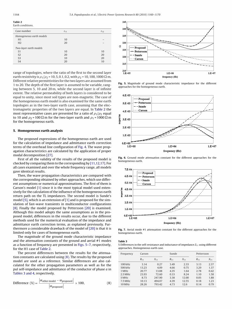
Fig. 5. Magnitude of ground mode characteristic impedance for the differentapproaches for the homogeneous earth.

Fig. 6. Ground mode attenuation constant for the different approaches for thehomogeneous earth.

Fig. 7. Aerial mode #1 attenuation constant for the different approaches for thehomogeneous earth.

Table 3% Differences in the self-resistance and inductance of impedance Z11 using differentapproaches. Homogeneous earth case.

Frequency Carson Sunde Pettersson

R11 X11 R11 X11 R11 X11

100 kHz 3.14 0.27 3.49 2.33 3.13 2.37500 kHz 13.23 4.09 4.66 0.75 3.29 1.37

S2 20 20S3 10 20S4 20 10

ange of topologies, where the ratio of the first to the second layerarth resistivity is �1/�2 = 10, 5, 0.1, 0.2, with �2 = 10, 100, 1000 � m.ifferent relative permittivities for the two layers are assumed fromto 20. The depth of the first layer is assumed to be variable, rang-

ng between 5, 10 and 20 m, while the second layer is of infinitextent. The relative permeability of both layers is considered to bequal to unity, since most soil types are non-magnetic. The case ofhe homogeneous earth model is also examined for the same earthopologies as in the two-layer earth case, assuming that the elec-romagnetic properties of the two layers are equal. In Table 2 the

ost representative cases are presented for a ratio of �1/�2 equalo 10 and �2 = 100 � m for the two-layer earth and �1 = 1000 � mor the homogeneous earth.

. Homogeneous earth analysis

The proposed expressions of the homogeneous earth are usedor the calculation of impedance and admittance earth correctionerms of the overhead line configuration of Fig. 4. The wave prop-gation characteristics are calculated by the application of properodal decomposition [27].First of all the validity of the results of the proposed model is

hecked by comparing them to the corresponding by [11,12,17]. Forll cases examined and over the whole frequency range, all modelsave identical results.

Then, the wave propagation characteristics are compared withhe corresponding obtained by other approaches, which use differ-nt assumptions or numerical approximations. The first of them isarson’s model [1] since it is the most typical model used exten-ively for the calculation of the influence of the homogeneous eartheturn path on the TL impedances. The second model is Sunde’sodel [5], which is an extension of [1] and is proposed for the sim-

lation of fast-wave transients in multiconductor configurations8]. Finally the model proposed by Pettersson [20] is examined.lthough this model adopts the same assumptions as in the pro-osed model, differences in the results occur, due to the differentethods used for the numerical evaluation of the impedance and

dmittance earth correction terms, as explained previously. Fur-hermore a considerable drawback of the model of [20] is that it isimited only for cases of homogeneous earth.

The magnitude of the ground mode characteristic impedancend the attenuation constants of the ground and aerial #1 modess a function of frequency are presented in Figs. 5–7, respectively,or the H1 case of Table 2.

The percent differences between the results for the attenua-ion constants are calculated using (8). The results by the proposed

odel are used as a reference. Similar differences are also cal-ulated for the other propagation parameters as well as for theul self-impedance and admittance of the conductor of phase a in

ables 3 and 4, respectively.

ifference (%) =∣∣˛other model − ˛proposed

∣∣∣∣˛proposed

∣∣ × 100, (8)

1 MHz 20.77 13.88 4.35 1.64 2.78 0.422.5 MHz 23.93 72.60 0.33 8.24 1.10 1.585 MHz 8.73 247.90 3.38 12.00 0.05 1.887.5 MHz 10.13 494.07 4.39 12.55 0.18 1.2310 MHz 28.26 793.42 4.73 12.6 0.14 0.79

T.A. Papadopoulos et al. / Electric Power Systems Research 80 (2010) 1160–1170 1165

Table 4% Differences in the self-conductance and susceptance of admittance Y11 using dif-ferent approaches. Homogeneous earth case.

Frequency Real part Imaginary part

100 kHz 11.08 0.01500 kHz 19.54 0.131 MHz 27.90 0.302.5 MHz 50.20 2.075 MHz 282.86 1.537.5 MHz 299.51 1.24

Acirf

mctai[i

irhptti

t3tasgs

iapn

T%H

quency of the first layer. In the high frequency region the groundmode characteristics by the two models show a completely differ-ent behavior.

10 MHz 329.83 1.10

s shown in Figs. 6 and 7, the ground and aerial mode attenuationonstants, calculated by the models of [1] and [5] are both monoton-cally increasing functions of frequency, while the correspondingesults calculated with the proposed model are non-monotoneunctions.

Differences in the modal propagation constants between theodels of Carson and the proposed are recorded for frequen-

ies higher than the minimum critical frequency fcr,min, which forhe examined case is 180 kHz. For frequencies up to 1 MHz arettributed mainly to the differences in the pul impedances as shownn Table 3, due to the omission of the influence of earth permittivity30], while for higher frequencies also due to the omission of themperfect earth on the shunt admittances.

In Sunde’s model the influence of earth permittivity is takennto account, thus differences in the modal attenuation constants,elated to the small differences in the pul impedances of Table 3,ave been reduced in the kHz range. The small differences in the pularameters are due to the omission of the displacement currents inhe air. However, the divergence of the results in the propagationerms in the MHz range is considerable, due to the omission of thenfluence of the imperfect earth on the shunt admittances.

The wave propagation characteristics obtained by [20] and byhe proposed model are almost identical for frequencies up toMHz, since differences do not overcome 10% for all wave parame-

ers, since the differences in the pul impedances and susceptancesre negligible. In the upper frequency range both models show theame behavior, while high differences are recorded mainly for theround attenuation constant, since significant differences in thehunt conductances are recorded, as shown in Table 4.

In Table 5, the relative differences in the propagation character-stics are shown for different homogeneous earth cases of Table 2,ssuming earth resistivity equal to 500 � m. Differences in the restropagation characteristics are not significant [32] and so they areot presented.

able 5Differences in the ground mode attenuation constant with different models.

omogeneous earth case.

Cases Frequencies

500 kHz 1 MHz 5 MHz 10 MHz

Carson’s modelH1 22.17 27.31 35.53 221.57H2 24.86 27.89 59.51 260.87

Sunde’s modelH1 13.15 14.14 60.95 199.71H2 10.05 6.89 56.82 150.56

Pettersson’s modelH1 5.4 6.4 22.3 51.75H2 5.01 4.83 17.17 43.08

Fig. 8. Magnitude of ground mode characteristic impedance for different two-layermethods.

6. Two-layer earth analysis

As in the homogeneous earth case, the modal propagation char-acteristics of the proposed method are compared to those obtainedby other approaches. The stratified earth topology for case S1,described previously, with depth of the first layer equal to 5 m isused in the following analysis.

First a simplified model is assumed, where both the influenceof the permittivity of the earth and the influence of the admit-tance earth correction terms are neglected. This model, which issimilar to Carson’s model but suitable for stratified cases, will becharacterized as “Low frequency (LF) Stratified earth model”.

The second model is a slight improvement to the latter in thehigh frequency range, since it takes into account only the effect ofthe air and the earth permittivities on the earth impedances. Thismodel is equivalent to that proposed by Nakagawa for the two-layerearth case.

The ground and aerial mode attenuation constants, calculatedby the three models are presented in Figs. 9 and 10, respectively.The corresponding curves of the LF Stratified model are mono-tonically increasing functions with frequency, much similar toCarson’s model for the homogeneous earth, since they both usethe same assumptions. For the ground mode, significant differencesare recorded for frequencies higher than the minimum critical fre-

Fig. 9. Ground mode attenuation constant for different two-layer methods.

1166 T.A. Papadopoulos et al. / Electric Power Systems Research 80 (2010) 1160–1170

F

teipsamap

ieTf�

7

l

•

•

•

•

•

T%l

penetration depth tends asymptotically to non-zero values evenin high frequencies, especially for cases of high earth resistivity.Therefore, although significant differences to the homogeneousearth case have been recorded for the earth return impedance [14]

ig. 10. Aerial mode #1 attenuation constant for different two-layer methods.

Although Nakagawa’s model is an improvement to the LF model,he differences with the proposed model still remain significant,specially in the high frequency region. This is due to the increas-ng influence of the admittance earth correction terms, since theroposed and Nakagawa’s models give identical results for theeries impedances. The ground mode attenuation curve presentslmost the same behavior as the corresponding of the LF Stratifiedodel up to several MHz. However, in the upper frequency rangemaximum peak point is recorded, due to the influence of earthermittivity on the series impedances.

The magnitude of the ground mode characteristic impedances shown in Fig. 8. The three models show a significant differ-nt behavior, leading to considerable differences in the result. Inable 6, the corresponding relative differences are shown for dif-erent two-layer earth cases of Table 2, assuming �1 = 500 � m and1 = 100 � m.

. Remarks on the numerical results.

Summarizing the analysis for the homogeneous and the two-ayer earth cases, the following remarks can be concluded.

Modal attenuation constants of the proposed models are non-monotone functions of frequency, since they present a maximumpeak value in the transition region.The proposed earth correction terms must be used for frequencieshigher than fcr,min of the homogeneous earth or of one of the twolayers.Carson’s formula for the homogeneous earth can be only used inthe low frequency region.

Sunde’s formulation for the homogeneous earth can be generallyused only up to 1 MHz in cases of high earth resistivity and highearth permittivity.Depending on the characteristics of the earth layers of the two-layer earth, resonant oscillations may be observed.

able 6Differences in the ground mode attenuation constant with different models. Two-

ayer earth case.

Cases Frequencies

500 kHz 1 MHz 5 MHz 10 MHz

LF statifiedH1 24.61 40.73 10.62 224.98H2 27.80 44.02 50.01 226.91

NakagawaH1 27.18 51.37 48.71 62.64H2 25.76 42.67 45.00 63.56

Fig. 11. Ground mode attenuation constants of the two-layer and homogeneousearth models.

8. Comparison of the two-layer with the homogeneousearth

The corresponding results for the stratified and the homoge-neous earth topologies are compared in order to check the influenceof earth stratification. For this purpose the proposed models for thetwo earth topologies, as well as the homogeneous earth and thetwo-layer earth models of Sunde and Nakagawa are chosen to beexamined.

For the two-layer earth topology the depth of the first layer isd = 5 m, earth resistivities are �1 = 1000 � m and �2 = 100 � m andthe relative permittivities of both layers are equal to 10, corre-sponding to case S1 of Table 2, while the homogeneous earth EMcharacteristics are assumed to be equal to those of the first layer,corresponding to case H1 of Table 2. The ground mode attenuationconstant is presented in Fig. 11.

The differences in the results by the proposed method betweenthe homogeneous and the stratified earth cases are shown in Fig. 12.They are calculated as percent using (8) with the homogeneousearth case as the reference. In the kHz frequency range differencesare in average over 30% and tend to minimize, until the correspond-ing curves in Fig. 11 intersect. For higher frequencies, althoughdifferences have been reduced, they still remain significant andreach 20%. This is better explained if we consider the field pene-tration depth [4], given by (9). Fig. 13 shows the variation of thepenetration depth with frequency and earth characteristics. The

Fig. 12. Differences in the ground mode attenuation constant between the stratifiedand the homogeneous earth models.

T.A. Papadopoulos et al. / Electric Power Systems Research 80 (2010) 1160–1170 1167

FR

afir

ı

9

lcm

mht

mhatitceolp

9

cstor

tardwt

need to include earth stratification in the transient transmissionline model.

The most severe transients have been observed in cases A, B andC for Nakagawa’s model, while in case D, the proposed two-layerearth model gives the worst transient. A direct interpretation of

ig. 13. Plot of the penetration depth vs. frequency for different earth resistivities.elative earth permittivity is 10.

nd shunt admittance [16] in the kHz frequency range, the strati-cation of earth must be taken into account in the high frequencyegion as well.

= 1

ω

√ε1�1/2(

√1 + (�2

1 /(ω2 · ε21)) − 1)

. (9)

. Transient responses

The propagation characteristics of the overhead transmissionine of Fig. 4 are used in the simulation of fast transients in order toheck the influence of the parameters, calculated by the proposedethodology on the transient response of the system.The wave propagation characteristics of the overhead trans-

ission line have been calculated for the same semi-infiniteomogeneous and two-layer earth models as previous, assuminghe same earth topologies and characteristics.

The time domain, distributed parameter traveling wave trans-ission line model of the ATP-EMTP [15] has been used. This model

as been modified, using a cascaded series of line sections anddding shunt lumped resistances to simulate the conductance ofhe admittance earth correction terms. In order to check the valid-ty of the modified model in high frequencies, results obtained forhe steady state case using this model, were checked to those cal-ulated by an exact frequency domain model using telegrapher’squations [19]. Negligible differences occurred, when the lengthf each cascaded equivalent line model is shorter than the wave-ength of the applied voltage and the time step of the simulationrocedure was is the order of nanoseconds.

.1. Modal responses

First the equivalent single-phase circuit of the ground mode isonsidered, for a line length equal to 5 km, to allow very fast tran-ients. A voltage step source with 1 pu magnitude is connected athe sending end S of the conductor, while the receiving end R ispen ended. In Fig. 14 the recorded transient voltages at the lineeceiving end are presented.

Differences in the transient responses between the stratified andhe homogeneous earth case are recorded, for both the proposednd the two approximate models. Comparing the proposed model

esults to the corresponding of Sunde and Nakagawa, significantifferences are recorded especially for the homogeneous earth case,hile for the stratified earth case the differences appear over a long

ime period.

Fig. 14. Ground mode receiving end step voltage of different models.

9.2. Actual phase responses

Next, for the investigation of the actual transmission line tran-sient response, the test configuration of Fig. 15 has been used.

The transmission line of Fig. 4 is considered with a length of1 km. A double exponential voltage source with a magnitude of 1 puand variable time constants is connected on the sending end S ofconductor of phase a. Each conductor open terminal is terminatedwith its characteristic impedance [27].

The examined test cases and the recorded absolute differencesin peak transient voltages indicating the quantitative influence ofthe different formulations are presented in Table 7. The percentdifferences are calculated keeping Sunde’s model as the referencein all cases, since it is commonly used in surge type simulations[8]. In Figs. 16 and 17 the recorded transient voltages at the linereceiving end R, for the different models are presented for the testcases A and D.

The comparison of the proposed model to Sunde’s model forthe homogeneous earth case leads to significant differences forcases B and D. These cases involve frequencies at the region wherethe modal propagation constants and especially the ground modeattenuation show a considerable divergence. The recorded differ-ences vary for the different test cases. Sunde’s model gives theworst transient in cases A and B, while in cases C and the proposedhomogeneous model presents the worst transient voltages.

Comparing the two stratified earth models, significant differ-ences on the transient voltages are also observed especially forthe test case D. Furthermore, the two stratified earth models resultin significantly different results to the homogeneous earth model,especially in cases of a very steep voltage ascent and therefore oftransients in the higher frequency range. These results justify the

Fig. 15. Test configuration of the transient simulation.

1168 T.A. Papadopoulos et al. / Electric Power Systems Research 80 (2010) 1160–1170

Table 7Peak relative (%) differences.

Test cases Front time/tail time (�s) % Differences

Proposed (homogeneous) Nakagawa (stratified) Proposed (stratified)

A 2/50 6.53B 1/50 11.28C 0.67/50 3.60D 0.5/50 33.59

Fig. 16. Receiving end transient voltages of different models for case A.

tptst

1

ttsirbw

acaa

′ −a |z−(d+h)| −a z

Fig. 17. Receiving end transient voltages of different models for case D.

he results is not easy, due to the complex differences in the modalropagation characteristics of the different models, especially inhe high frequencies. However, the recorded differences in the tran-ient responses justify the need for a more precise estimation of theransmission line model parameters.

0. Conclusion

A generalized formulation for the calculation of the influence ofhe imperfect earth on the series impedances and shunt admit-ances of overhead transmission lines in high frequencies fortratified earth cases is presented in this paper. Special emphasiss given to the influence of the axial displacement currents and theadial displacement and conducting currents. These currents muste taken into account in the high frequency region, the range ofhich depends on the electromagnetic characteristics of the earth.

The proposed generalized expressions, derived under thessumption of quasi-TEM propagation, can handle all practi-al cases of overhead multiconductor arrangements, taking intoccount the topology and the electromagnetic properties ofll involved media. These expressions can include all existing

19.11 12.8228.54 4.4429.46 24.5525.38 61.73

approaches for the homogeneous and the two-layer earth cases,by the application of the corresponding assumptions. Finally, theymay be also extended to include multi-layer horizontally stratifiedearth structures.

The propagation characteristics of a typical single-circuit three-phase overhead TL configuration has been analyzed for severalearth topologies of arbitrary EM characteristics for a frequencyrange from 50 Hz to 10 MHz. The validity and accuracy of the pro-posed model has been verified, by comparing the obtained resultswith the corresponding by other known approaches.

From the comparative analysis of the results, it is shown thatthe influence of the earth permittivity for the line impedances andadmittances must be taken into account. This is most evident incases where the earth does not behave as a conductor but also asan insulator. Furthermore, earth stratification must be not omittedin the simulation of high frequency phenomena, especially whenthe penetration depth of the EM field extends deeper than the upperearth layer.

Finally, the influence of the parameters calculated by the pro-posed model on the transient response of a transmission line ischecked, by simulating typical fast transient surges. Results showthat the new correction terms introduced by the proposed modelshave a significant influence on the transient responses, especiallyin the MHz frequency range.

The proposed theoretical model together with the numericalintegration scheme can be used for any type of overhead line config-uration, offering a useful tool in the calculation of parameters of fasttransient overhead line models and thus enhancing the simulationof various earth structures.

Acknowledgements

This work was supported by the Greek General Secretariat forResearch and Technology (PENED 03). The helpful recommen-dations of Dr. D.A. Tsiamitros are greatly acknowledged by theauthors.

Appendix A.

A.1. Determination of the dipole EM field

We assume a dipole with a moment IdS along the x-axis, placedin the height h = hi of conductor i over a two-layer earth, as shown inFig. 18. Since the field is symmetrical with respect to the x–z plane,the y component ˘ ′

y is zero. The x- and z-components of the resul-tant Herzian vector in the air, the first layer and the second layerare ˘ ′

0x, ˘ ′0z , ˘ ′

1x, ˘ ′1z and ˘ ′

2x, ˘ ′2z , respectively. Their analytical

expressions are:

A.1.1. Air (z ≥ d)∫ ∞ [u ′ ′

]

˘0x =

0

Ca′

0e 0 + g0 · e 0 J0(ru)du, (A.1a)

˘ ′0z = x

r

∫ ∞

0

p0 · e−a′0

z · J1(ru)du. (A.1b)

T.A. Papadopoulos et al. / Electric Power Sys

A

˘

˘

A

˘

˘

Ioar

2v

fbg

�

Tzat(a(

g

p

Tc

T

Fig. 18. Dipole configuration over a two-layer earth.

.1.2. First earth layer (0 ≤ z < d)

′1x =

∫ ∞

0

[f1 · ea′

1z + g1 · e−a′

1z]

J0(ru)du, (A.2a)

′1z = x

r

∫ ∞

0

[p1 · ea′

1z + q1 · e−a′

1z]

J1(ru)du. (A.2b)

.1.3. Second earth layer (z < 0)

′2x =

∫ ∞

0

f2 · ea′2

z · J0(ru)du, (A.3a)

′2z = x

r

∫ ∞

0

p2 · ea′2

z · J1(ru)du. (A.3b)

n the above equations, the prime indicates the Herzian vectorf the dipole, as opposed to that of an infinite line. J0( ) and J1( )re the Bessel functions of the first kind and zero and first order,espectively, �2

k= jω�k(�k + jωεk), a′

k=√

u2 + �2k

, where k = 0, 1,

, r =√

x2 + y2, cos ϕ = x/r, j is the imaginary unit, u the integralariable and C is equal to I · dS · jω�0/4��2

0 .The unknown functions f and g in Eqs. (A.1)–(A.3) are obtained

rom the boundary conditions between the different media. Theoundary conditions between two horizontal media a and b areenerally defined as [14]:

2a · ˘ ′

ax = �2b · ˘ ′

bx, (A.4a)

�2a

�a· ∂˘ ′

ax

∂z= �2

b

�b· ∂˘ ′

bx

∂z, (A.4b)

�2a

�a˘ ′

az = �2b

�b˘ ′

bz, (A.4c)

∂˘ ′ax

∂x+ ∂˘ ′

az

∂z= ∂˘ ′

bx

∂x+ ∂˘ ′

bz

∂z. (A.4d)

he above set of equations is applied to each separating surface at= d and z = 0. First, the x-components are determined separatelynd then are used in finding the z-components. Therefore, substi-uting (A.1a), (A.2a), and (A.3a) in (A.4a) and (A.4b) and also (A.1b),A.2b), and (A.3b) in (A.4c) and (A.4d) the unknown functions g0nd p0 of (A.1a) and (A.1b), respectively are derived in (A.5a) andA.5b).

0 = Cu

a0· e−a′

0(h−d) · T ′

1, (A.5a)

0 = 2Cu2 · e−a′0

(h−d) · T ′2, (A.5b)

′ and T ′ are given in (A.6a) and (A.6b), respectively, while their

1 2omponents are presented in (A.7).

′1 = ′

1′ = d′

01s′12 + s′

01d′12e−2a′

1d

s′01s′

12 + d′01d′

12e−2a′1

d, (A.6a)

tems Research 80 (2010) 1160–1170 1169

T ′2 =

�0�1(�20 − �2

1 )[s′12 + d′

12e−2a′1

d][S′12 + D′

12e−2a1d]

−4�0�21�2a′2

1�20 e−2a1d(�2

2 − �21 )

′2 · ′ , (A.6b)

′ = s′01s′

12 + d′01d′

12e−2a′1

d, (A.7a)

1 = d′01s′

12 + s′01d′

12e−2a′1

d, (A.7b)

′2 = S′

01S′12 + D′

01D′12e−2a1d. (A.7c)

s′mn = (a′

m�n + a′n�m), (A.7d)

d′mn = (a′

m�n − a′n�m), (A.7e)

S′mn = (�m�2

n a′m + �n�2

ma′n), (A.7f)

D′mn = (�m�2

n a′m − �n�2

ma′n), (A.7g)

where the m, n indices, take the values 0, 1, 2, corresponding to theair and the two earth layers, respectively.

Thus, the ˘ ′ function in the air is completely defined and (A.1a)and (A.1b) take the following respective form:

˘ ′0x =

∫ ∞

0

(Cu

a′0

e−a′0|z−(d+h)| + Cu

a′0

e−a′0

(h+z−d) · T ′1

)J0(ru)du, (A.8a)

˘ ′0z = x

r

∫ ∞

0

2Cu2 · T ′2 · e−a′

0(h+z−d)J1(ru)du. (A.8b)

Next, the x and y components of the electric field intensity areexpressed in rectangular coordinates and are defined by the wavefunction ˘ and the intermediate functions P(r) and Q(r) in (A.9a)and (A.9b) [5].

Ex= − �20 ˘ ′

0x+∂

∂x

[∂˘ ′

0x

∂x+∂˘ ′

0z

∂z

]= IdS

[−P(r) + ∂2Q (r)

∂x2

], (A.9a)

Ey = ∂

∂y

[∂˘ ′

0x

∂x+ ∂˘ ′

0z

∂z

]= IdS

∂2Q (r)∂x∂y

, (A.9b)

P(r) and Q(r) are used in the determination of the pul earth cor-rection terms of a line with an infinite length in the followingexpressions [5]:

Z ′eij

(�x) =∫ ∞

−∞P(√

x2 + y2)e−�xxdx, (A.10a)

Y′−1eij

(�x) =∫ ∞

−∞Q (√

x2 + y2)e−�xxdx, (A.10b)

Substituting in (A.9) Eqs. (A.8a) and (A.8b) and using (A.11), (4a)and (4b) are derived.

∂J0(ru)∂x

= −cos ϕ · u · J1(ru), (A.11)

A.2. Derivation of the impedance and admittance formulas

Since �x is equal to jk0, the second integral of (4) can be calcu-lated using (A.9) [14].∫ ∞

−∞J0

(u√

x2 + y2ij

)e−jk0xdx

=

⎧⎪⎨⎪⎩

0, u < k0

2cos(

yij

√u2 − k2

0

)√ , u > k0

, (A.12)

u2 − k20

Assuming the relation u2 − k20 = 2, the terms a′

kfor k = 0, 1, 2 trans-

form to ak =√

2 + �2k

+ k20, T ′

1 and T ′2 to T1 and T2, respectively.

Using (A.9) and the above transformations the pu length mutual

1 er Sys

ita∫

w

R

[

[

[

[

[

[

[

[

[

[

[

[

[

[

[

[

[

[

[

[

[

[

[

Computer Engineering at the Aristotle University of Thessaloniki, in 1981 and 1989,

170 T.A. Papadopoulos et al. / Electric Pow

mpedances and admittances for the two-layer earth structure takehe form of (5) and (6), respectively. The logarithmic terms of (5)nd (6) are derived, using (A.10) [14].

∞

0

(e

−˛′0

∣∣hj−hi

∣∣a′

0+ e−˛′

0(hi+hj)

a′0

)cos (yij)d = ln

Dij

dij, (A.13)

here Dij =√

y2ij

+ (hi + hj)2, dij =

√y2

ij+ (hi − hj)

2.

eferences

[1] J.R. Carson, Wave propagation in overhead wires with ground return, Bell Syst.Tech. J. (5) (1926) 539–554.

[2] M.C. Perz, M.R. Raghuveer, Generalized derivation of fields, and impedancecorrection factors of lossy transmission lines. Part II. Lossy conductors abovelossy ground, IEEE Trans. Power Syst. 93 (6) (1974) 1832–1841.

[3] L. Hofman, Series expansions for line series impedances considering differentspecific resistances, magnetic permeabilities, and dielectric permittivities ofconductors, air, and ground, IEEE Trans. Power Deliv. 18 (2) (2003) 564–570.

[4] A. Semlyen, Ground return parameters of transmission lines an asymptoticanalysis for very high frequencies, IEEE Trans. Power Syst. 100 (3) (1981)1031–1038.

[5] E.D. Sunde, Earth Conduction Effects in Transmission Systems, 2nd ed., DoverPublications, 1968, pp. 99–139.

[6] F. Rachidi, C.A. Nucci, M. Ianoz, Transient analysis of multiconductor lines abovea lossy ground, IEEE Trans. Power Deliv. 14 (1) (1999) 294–302.

[7] N. Theethayi, R. Thottappillil, Y. Liu, R. Montano, Important parameters thatinfluence crosstalk in multiconductor transmission lines, Electr. Power Syst.Res. (2006), doi:10.1019/j.epsr.2006.06.014.

[8] F. Rachidi, C.A. Nucci, M. Ianoz, C. Mazzeti, Influence of a lossy ground onlightning-induced voltages on overhead lines, IEEE Trans. EMC 38 (3) (1996)250–264.

[9] W.H. Wise, Propagation of high frequency currents in ground return circuits,Proc. Inst. Radio Eng. (22) (1934) 522–527.

10] W.H. Wise, Effect of ground permeability on ground return circuits, Bell Syst.Tech. J. (10) (1931) 472–484.

11] W.H. Wise, Potential coefficients for ground return circuits, Bell Syst. Tech. J.27 (1948) 365–371.

12] M. Nakagawa, Admittance correction effects of a single overhead line, IEEETrans. Power Syst. PAS-100 (3) (1981) 1154–1161.

13] M. Nakagawa, Further Studies on wave propagation along overhead transmis-sion lines: effects of admittance correction, IEEE Trans. Power Syst. PAS-100 (7)(1981) 3626–3633.

14] N. Nakagawa, A. Ametani, K. Iwamoto, Further studies on wave propagation inoverhead lines with earth return: impedance of stratified earth, Proc. IEE 120(12) (1973) 1521–1528.

15] H.W. Dommel, Electromagnetic Transients Program Reference Manual, Bon-neville Power Administration, Portland, OR, 1986.

16] A. Ametani, N. Nagaoka, R. Koide, Wave propagation characteristics on an over-head conductor above snow, Trans. Inst. Electr. Eng. Jpn. 134 (3) (2001) 26–33.

17] H. Kikuchi, Wave propagation along an infinite wire above ground at high

frequencies, Electrotech. J. Jpn. 2 (1956) 73–78.

18] A.E. Efthymiadis, L.M. Wedepohl, Propagation characteristics of infinitely – longsingle – conductor lines by the complete field solution method, Proc. IEE 125(6) (1978) 511–517.

19] F.M. Tesche, M. Ianoz, T. Karlsson, EMC Analysis methods and ComputationalModels, John Wiley and Sons Inc., 1997, pp. 405–411.

tems Research 80 (2010) 1160–1170

20] P. Pettersson, Image representation of wave propagation on wires above, onand under ground, IEEE Trans. Power Deliv. 9 (2) (1994) 1049–1055.

21] M. D’Amore, M.S. Sarto, Simulation models of a dissipative transmission lineabove a lossy ground for a wide-frequency range. Part I: Single conductor con-figuration, IEEE Trans. EMC 38 (2) (1996) 127–138.

22] M. D’Amore, M.S. Sarto, Simulation models of a dissipative transmission lineabove a lossy ground for a wide-frequency range. Part II: Multiconductor con-figuration, IEEE Trans. EMC 38 (2) (1996) 139–149.

23] J.R. Wait, Theory of wave propagation along a thin wire parallel to an interface,Radio Sci. 7 (6) (1972) 675–679.

24] P. Degauque, G. Courbet, M. Heddebaut, Propagation along a line parallel to theground surface: comparison between the exact solution and the quasi-TEMapproximation, IEEE Trans. EMC vol.25 (4) (1983) 422–427.

25] G.E.J. Bridges, L. Shafai, Plane wave coupling to multiple conductor tranmissionlines above a lossy earth, IEEE Trans. EMC vol.31 (1) (1989) 21–33.

26] G.K. Papagiannis, D.A. Tsiamitros, D.P. Labridis, P.S. Dokopoulos, A system-atic approach to the evaluation of the influence of multilayered earth onoverhead power transmission lines, IEEE Trans. Power Deliv. 20 (4) (2005)2594–2601.

27] L.M. Wedepohl, Application of the solution of travelling wave phenomena inpolyphase system, Proc. IEE 110 (December (12)) (1963) 2200–2212.

28] A. Ametani, A general formulation of impedance and admittance of cables, IEEETrans. Power Appar. Syst. PAS-99 (3) (1980) 902–910.

29] R.G. Olsen, J.L. Young, D.C. Chang, Electromagnetic wave propagation ona thin wire above earth, IEEE Trans. Antennas Propag. 48 (9) (2000)1413–1419.

30] T.A. Papadopoulos, G.K. Papagiannis, “Influence of Earth Permittivity on Over-head Transmission Line Earth-Return Impedances,” presented at 2007 IEEELausanne PowerTech Conf., Lausanne, Switcherland, 2007.

31] P. Amirshahi, M. Kavehrad, High-Frequency characteristics of overhead multi-conductor power lines for broadband communications, IEEE J. Selected AreasCommun. 24 (7) (2006).

32] A. Ametani, Stratified earth effects on wave propagation—frequency-dependent parameters, IEEE PAS PAS-93 (5) (1974) 1233–1239.

Theofilos A. Papadopoulos was born in Thessaloniki, Greece, on March 10, 1980. Hereceived his Dipl. Eng. Degree from the Department of Electrical and ComputerEngineering at the Aristotle University of Thessaloniki, in 2003. Since 2003 he isa postgraduate student at the Department of Electrical and Computer Engineeringat the Aristotle University of Thessaloniki. His special interests are power systemsmodeling, power-line communications and computation of electromagnetic tran-sients. Mr. Papadopoulos has received the Basil Papadias Award for the best studentpaper, presented at the IEEE PowerTech ’07 Conference in Lausanne, Switzerland.

Grigoris K. Papagiannis was born in Thessaloniki, Greece, on September 23, 1956. Hereceived his Dipl. Eng. Degree and his Ph.D. degree from the Department of Electricaland Computer Engineering at the Aristotle University of Thessaloniki, in 1979 and1998, respectively.

He is currently As. Professor at the Power Systems Laboratory of the Departmentof Electrical and Computer Engineering of the Aristotle University of Thessaloniki,Greece. His special interests are power systems modeling, computation of electro-magnetic transients, distributed generation and power-line communications.

Dimitris P. Labridis was born in Thessaloniki, Greece, on July 26, 1958. He receivedthe Dipl.-Eng. degree and the Ph.D. degree from the Department of Electrical and

respectively. Currently he is a Professor at the same Department. His special interestsare power system analysis with special emphasis on the simulation of transmissionand distribution systems, electromagnetic and thermal field analysis, artificial intel-ligence applications in power systems, power-line communications and distributedenergy resources.