Nonlinear coupling control laws for an overhead crane system

Nonlinear Coupling Control Laws for a 3-DOF Overhead Crane

System*

Y. Fang1, W. E. Dixon2, D. M. Dawson1, E. Zergeroglu3 1Department of Electrical and Computer Engineering, Clemson University, Clemson, SC 29634-0915

2Robotics and Process Systems Division, Oak Ridge National Laboratory, P.O. Box 2008, Oak Ridge, TN 37831-6305 3Lucent Technologies, Bell Lab Innovations Optical Fiber Solutions, 50 Halls Rd, Sturbridge MA, 01566

E-mail: [email protected], Telephone: (865) 574-9025

Keywords: Overhead Crane, Nonlinear Control Application, Underactuated, Setpoint Regulation

"The submitted manuscript has been authored by a contractor of the U.S. Government under contract No. DE-AC05-96OR22464. Accordingly, the U.S. Government retains a nonexclusive, royalty-free license to publish or reproduce the published form of this contribution, or allow others to do so, for U.S. Government purposes."

Submitted to the IEEE Conference on Decision and Control, Dec. 4-7, 2001, Orlando, Florida

* This research was performed in part by a Eugene P. Wigner Fellow and staff member at the Oak Ridge National Laboratory, managed by UT-Battelle, LLC, for the U.S. Department of Energy under contract DE-AC05-00OR22725 and is supported in part by the U.S. NSF Grants DMI-9457967, DMI-9813213, EPS-9630167, ONR Grant N00014-99-1-0589, a DOC Grant, and an ARO Automotive Center Grant.

Nonlinear Coupling Control Laws for a 3-DOF OverheadCrane System∗

Y. Fang1, W. E. Dixon2, D. M. Dawson1, and E. Zergeroglu31Department of Electrical & Computer Engineering, Clemson University, Clemson, SC 29634-09152Oak Ridge National Laboratory, P.O. Box 2008, Bldg. 7601, Mailstop 6305, Oak Ridge, TN 37831

3Lucent Technologies, Bell Lab Innovations Optical Fiber Solutions, 50 Halls Rd, Sturbridge MA, 01566

email: yfang, [email protected], [email protected], [email protected]

Abstract

In this paper, we consider the regulation control problem for a three-degree-of-freedom (3-DOF), underactuated overhead crane system. Motivated by recent passivity-based controllersfor underactuated systems, we design several controllers that asymptotically regulate the planargantry position and the payload angle. Specifically, utilizing LaSalle’s Invariant Set Theorem,we first illustrate how a simple proportional-derivative (PD) controller can be utilized to as-ymptotically regulate the overhead crane system. Motivated by the desire to achieve improvedtransient performance, we then design two nonlinear controllers that increase the couplingbetween the planar gantry position and the payload angle.

1 IntroductionPrecise payload positioning by an overhead crane (especially when performed by a operator usingonly visual feedback to position the payload) is difficult due to the fact that the payload can exhibita pendulum-like swinging motion. These payload swings can result in several performance andsafety concerns including: i) damage to the payload (e.g., spillage or breakage), ii) damage tothe surrounding environment or personnel, and iii) large internal forces that can result in reducedpayload carrying capacity or premature failure of stressed parts. Motivated by the desire to achievefast and precise payload positioning while mitigating the above performance and safety concerns,several researchers have developed various controllers for overhead crane systems. For example,Yu et al. [16] utilized a time-scale separation approach to control a two degree-of-freedom (2-DOF) overhead crane system; however, an approximate linearized model of the crane was utilizedto facilitate the construction of the error systems. In [15], Yashida et al. proposed a saturatingcontrol law based on a guaranteed cost control method for a linearized version of the 2-DOF cranesystem dynamics. Martindale et al. [9] utilized an approximate crane model to develop exactmodel knowledge and adaptive controllers while Butler et al. [2] exploited a modal decomposition∗This research was performed in part by a Eugene P. Wigner Fellow and staff member at the Oak Ridge National

Laboratory, managed by UT-Battelle, LLC, for the U.S. Department of Energy under contract DE-AC05-00OR22725and is supported in part by the U.S. NSF Grants DMI-9457967, DMI-9813213, EPS-9630167, ONR Grant N00014-99-1-0589, a DOC Grant, and an ARO Automotive Center Grant.

1

technique to develop an adaptive controller. In [3], Chung and Hauser designed a nonlinear controllerfor regulating the swinging energy of the payload.Several researchers have also examined the control problem for 3-DOF overhead crane systems.

Specifically, Moustafa and Ebeid [10] derived the nonlinear dynamic model for a 3-DOF overheadcrane and then utilized a standard linear feedback controller based on a linearized state space model.In [11], Noakes and Jansen developed a generalized input shaping approach for the linearized cranedynamics that exploited a notch filtering technique to control the motion of the bridge/trolley ofa 3-DOF overhead crane system. More recently, Lee [7] developed a nonlinear model for 3-DOFoverhead cranes based on a new 2-DOF swing angle definition. Based on this nonlinear model, Leethen developed an anti-swing control law for the decoupled linearized dynamics. In [12], Sakawaand Sano derived a nonlinear model for a 3-DOF crane system that was subsequently linearizedto facilitate the development of a control scheme that first transferred the load to a position nearthe equilibrium point using an open-loop controller and then utilized a linear feedback controller tostabilize the payload about the equilibrium point.One of the limiting factors associated with the above overhead crane control designs is that

the system nonlinearities are often excluded from the closed-loop error system design and stabilityanalysis. To overcome this drawback, several researchers have investigated control approaches thataccount for the nonlinear dynamics of overhead cranes and similar systems. For example in [14],Teel utilized saturation functions to develop an output feedback controller which achieves a robust,semi-global stability result for the ball-and-beam control problem. In [1], Burg et al. transformedthe nonlinear crane dynamics into a structure that resembled the ball-and-beam problem and thenadopted the research efforts of [14] to achieve asymptotic positioning from a large set of initial con-ditions. More recently, Fantoni et al. [5] and Lozano et al. [8] proposed passivity-based controllersfor the inverted pendulum and the pendubot (i.e., an inverted pendulum-like robot with an unactu-ated second link) based on the paradigm of driving the underactuated system to a homoclinic orbitusing an energy-based nonlinear controller and then switching to a linear controller to stabilize thesystem around its unstable equilibrium point. Using similar stability analysis techniques, Colladoet al. [4] proposed a proportional-derivative (PD) controller for the overhead crane problem. In[6], Kiss et al. developed a PD controller for a vertical crane-winch system that only requires themeasurement of the winch angle and its derivative rather than a cable angle measurement.In this paper, we utilize a similar approach as provided by [8] to develop several controllers

for the 3-DOF overhead crane system. Specifically, utilizing LaSalle’s Invariant Set Theorem, weillustrate how a simple PD controller can be utilized to asymptotically regulate the overhead cranedynamics. Motivated by the desire for improved transient response, we design two nonlinear energy-based coupling control laws that increase the coupling between the pendulum position and thegantry position. Simulation results are provided, which illustrate that the increased coupling ofthe nonlinear controllers results in improved transient response (e.g., reduced overshoot and fastersettling time) over the PD control law. The paper is organized as follows. In Section 2, we presentthe nonlinear dynamic model of the overhead crane system and in Section 3, we rewrite the open-loop system into a more convenient form. In Section 4, we develop a PD controller and two nonlinearcontrollers and examine the stability of the controllers through a Lyapunov-like stability analysis.The performance of the proposed controllers is illustrated through simulation results presented inSection 5. Concluding remarks are given in Section 6.

2

2 Dynamic ModelThe dynamic model for a three degree-of-freedom (3-DOF) overhead crane system (see Figure 1) isassumed to have the following form [10]

M(q)q + Vm(q, q)q +G(q) = u (1)

where q(t) ∈ R4 is defined as follows

q = [x y θ φ]T (2)

where x(t) ∈ R1 denotes the gantry position along the X-Coordinate axis, y(t) ∈ R1 denotes thegantry position along the Y -Coordinate axis, θ(t) ∈ R1 denotes the payload angle with respect tothe vertical, φ(t) ∈ R1 denotes the projection of the payload angle along the X-Coordinate axis,and M(q) ∈ R4×4, Vm(q, q) ∈ R4×4, G(q) ∈ R4, and u(t) ∈ R4 are defined as follows

M =

mp +mr +mc 0 mpL cos θ sinφ mpL sin θ cosφ

0 mp +mc mpL cos θ cosφ −mpL sin θ sinφmpL cos θ sinφ mpL cos θ cosφ mpL

2 + I 0mpL sin θ cosφ −mpL sin θ sinφ 0 mpL

2 sin2 θ + I

(3)

Vm =

0 0 −mpL sin θ sinφθ +mpL cos θ cosφφ mpL cos θ cosφθ −mpL sin θ sinφφ

0 0 −mpL sin θ cosφθ −mpL cos θ sinφφ −mpL cos θ sinφθ −mpL sin θ cosφφ

0 0 0 −mpL2 sin θ cos θφ

0 0 mpL2 sin θ cos θφ mpL

2 sin θ cos θθ

(4)

G = [0 0 mpgL sin θ 0]T (5)

u = [Fx Fy 0 0]T (6)

where mp,mr,mc ∈ R1 represent the payload mass, rail mass, and cart mass, respectively, I ∈ R1denotes the moment of inertia of the payload, L ∈ R1 represents the length of the crane rod, g ∈ R1represents the gravity effects, and Fx(t), Fy(t) ∈ R1 represent the control force inputs acting on thecart and rail, respectively. Based on the structure of M(q) and Vm(q, q) given in (3) and (4), it isstraightforward to show that the following skew-symmetric relationship is satisfied

ξTµ1

2M(q)− Vm(q, q)

¶ξ = 0 ∀ ξ ∈ R4 (7)

where M(q) represents the time derivative of M(q) and that the inertia matrix M(q) can be upperand lower bounded by the following inequalities

k1 kξk2 ≤ ξTM(q)ξ ≤ k2 kξk2 ∀ξ ∈ R4 (8)

where k1, k2 ∈ R1 are positive bounding constants. In a similar manner as in [1] and [9], we assumethat the dynamic model given in (1) has the following characteristics.

Assumption 1: The payload and the gantry are connected by a massless, rigid link.

Assumption 2: The angular position and velocity of the payload and the planar position andvelocity of the gantry are measurable.

3

Assumption 3: The gantry mass and the length of the connecting rod are exactly known.

Assumption 4: The ball joint that connects the payload link to the gantry is frictionless and thatthis joint does not rotate about the connecting rod (i.e., the payload does not rotate aboutthe rod axis).

Assumption 5: The angular position of the payload mass is restricted according to followinginequality

−π

2< θ(t) <

π

2(9)

where θ(t) is measured from the vertical position (see Figure 1).

XY

Z

mr

XYZ: Fixed coordinate system

mc

mp

θ

φφφφ

Figure 1: 3-DOF Overhead Crane System

Remark 1 Note that the model given by (1) could be modified to include other dynamic effects as-sociated with the gantry dynamics (e.g., gantry friction, viscous damping coefficients, mass momentof inertia of the gantry and rail motors, etc.); however, these additional dynamic effects were notincluded in the model since these effects can be directly cancelled by the controller.

3 Open-Loop System DevelopmentTo express (1) in a form that facilitates the subsequent control development and stability analysis,we premultiply both sides of (1) by M−1(q) to obtain the following expression

q =M−1 (u− Vmq −G) (10)

where M−1(q) ∈ R4×4 is guaranteed to exist due to the fact that the determinant of M(q), denotedby det(M), is a positive function as shown below

det(M) = I2 (mp +mc) (mp +mr +mc) +mpL2I£(mp +mr +mc)mc

¡1 + sin2 θ

¢(11)

+(mp +mc)mp sin2 θ +mrmp

¡sin2 φ+ 2 sin2 θ cos2 φ

¢¤+m2

pL4 sin2 θ

¡mrmp sin

2 θ cos2 φ+mc

¡mr +mc +mp sin

2 θ¢¢.

4

After substituting (3), (4), (5), (6) and the expression for M−1(q) into (10) and performing somealgebraic manipulation, we can rewrite (10) as follows

x =1

det(M)(p11Fx + p12Fy + w1) (12)

y =1

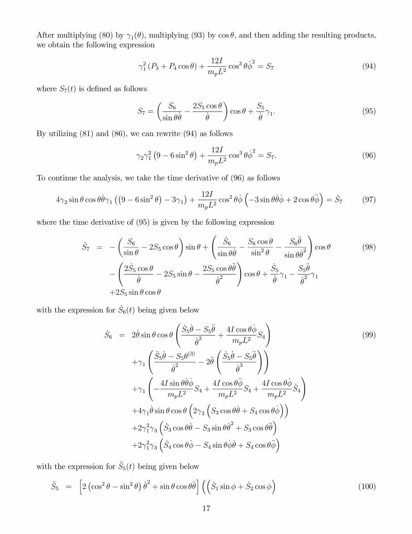
det(M)(p12Fx + p22Fy + w2) (13)

where the measurable auxiliary terms p11(q), p12(q), p22(q), w1(q, q), w2(q, q) ∈ R1 are defined asfollows

p11 = m2pL

2I¡sin2 φ+ 2 sin2 θ cos2 φ

¢+mpI

2 +mcmpL4 sin2 θ (14)

+mcmpL2I¡1 + sin2 θ

¢+mcI

2 +m3pL

4 cos2 φ sin4 θ

p12 = −m3pL

4 sinφ cosφ sin4 θ −m2pL

2I sinφ cosφ¡sin2 θ − cos2 θ¢ (15)

p22 = m3pL

4 sin4 θ sin2 φ+m2pL

2I£1 +

¡sin2 θ − cos2 θ¢ sin2 φ¤ (16)

+(mp +mr +mc) I2 + (mr +mc)m

2pL

4 sin2 θ

+(mr +mc)mpL2I¡1 + sin2 θ

¢w1 = mpL sin θ sinφ

£(mp +mc) I +mpmcL

2 sin2 θ¤

(17)hφ2 ¡mpL

2 sin2 θ + I¢+ θ

2 ¡mpL

2 + I¢i

−2ImpLθφ cos θ cosφ£(mp +mc) I +mpL

2¡mc +mp sin

2 θ¢¤

+m2pgL

2 sin θ cos θ sinφ£(mp +mc) I +mpmcL

2 sin2 θ¤

w2 = mpL sin θ cosφ£(mp +mr +mc) I + (mr +mc)mpL

2 sin2 θ¤

(18)£d2¡mpL

2 sin2 θ + I¢+ p2

¡mpL

2 + I¢¤

+2mpLI θφ cos θ sinφ£(mp +mr +mc)

¡mpL

2 + I¢−m2

pL2 cos2 θ

¤+mpgL sin θ

£(mr +mc)m

2pL

3 sin2 θ cos θ cos φ

+(mr +mc +mp)mpLI cos θ cosφ] .

In order to write the open-loop dynamics given in (12) and (13) in a more compact form for thesubsequent control development and stability analysis, we define the auxiliary signal r(t) ∈ R2 asfollows

r = [x y]T . (19)

After taking the second time-derivative of r(t) and then utilizing the expressions given in (12)-(18),we can rewrite the open-loop dynamics given in (12) and (13) as follows

r =

·xy

¸=

1

det(M)(PF +W ) (20)

where P (q) ∈ R2×2 and W (q, q) ∈ R2 are defined as follows

P =

·p11 p12p12 p22

¸W =

·w1w2

¸(21)

5

and F (t) ∈ R2 is defined belowF = [Fx Fy]

T . (22)

Given the expressions in (14)-(16), it is straightforward to prove that

p11 > 0 and p11p22 − p212 ≥ mp (mp +mr +mc) I4. (23)

From the expressions given in (21) and (23), we can see that P (q) is positive-definite, symmetric,and invertible, where the inverse of P (q), denoted by P−1(q), is also positive-definite and symmetric.To facilitate the subsequent Lyapunov-based control design, we will utilize the energy of the

overhead system, denoted by E(q, q) ∈ R1, and defined as follows

E(q, q) =1

2qTM(q)q +mpgL(1− cos(θ)) ≥ 0. (24)

After taking the time derivative of (24), substituting (1) forM(q)q(t), and canceling common terms,we obtain the following expression for the time derivative of E(q, q)

E = rTF (25)

where (3), (4), and (7) were utilized.

4 Control Design and AnalysisOur control objective is the regulation of the planar gantry position of the overhead crane to aconstant desired position, denoted by rd ∈ R2, which is explicitly defined as

rd = [xd yd]T . (26)

In addition, the payload angle θ(t) must also be regulated to zero. To quantify the control objectiveof regulating the overhead crane to a constant desired position, we define a gantry position errorsignal e(t) ∈ R2 as follows

e(t) = r − rd. (27)

In the subsequent control development, we will design a proportional-derivative control law and twononlinear controllers to achieve the above control objective.

Remark 2 The control objective is defined in terms of regulating the gantry position and the angleof the payload with the vertical. The problem of regulating the projection of the payload angle alongthe X-Coordinate axis, denoted by φ(t), is not required. That is, if the payload angle, denoted byθ(t), is regulated to zero, then we can see from Figure 1 that the payload has been regulated to thedesired location.

4.1 Proportional-Derivative Control Law

Based on the subsequent stability analysis, we design the following proportional-derivative (PD)control law

F =−kpe− kdr

kE(28)

where kd, kE, kp ∈ R1 are positive constant control gains.

6

Theorem 1 The controller given in (28) ensures asymptotic regulation of the overhead crane sys-tem in the sense that

limt→∞

¡x(t) y(t) θ(t)

¢=¡xd yd 0

¢(29)

where xd and yd were defined in (26).

Proof: To prove (29), we define a nonnegative function V1(t) ∈ R1 as follows

V1 = kEE +1

2kpe

T e. (30)

After taking the time derivative of (30) and then substituting (25) and the time derivative of (27)into the resulting expression, we can rewrite (30) as follows

V1 = rT (kEF + kpe) . (31)

After substituting (28) into (31) for F (t) and then cancelling common terms, we obtain the followingexpression

V1 = −kdrT r. (32)

Based on the expressions given in (8), (24), (27), (30) and (32), it is clear that the origin of theclosed-loop system is stable in the sense of Lyapunov [13] and that r(t), e(t), q(t) ∈ L∞. Based on thefact that r(t), e(t), q(t) ∈ L∞, we can utilize (2) and (19) to prove that x(t), x(t), y(t), y(t), r(t), θ(t),φ(t) ∈ L∞. Given that e(t), r(t) ∈ L∞, it is clear from (28) that F (t) ∈ L∞. Finally, from (6) and(22), we can prove that Fx(t), Fy(t), u(t) ∈ L∞.Based on the fact that all of the closed-loop signals remain bounded, we can now employ LaSalle’s

Invariance Theorem to prove (29). To this end, we define Γ as the set of all points where

V1 = 0. (33)

In the set Γ, it is clear from (32) and (33) that

r(t) = 0 r(t) = 0, (34)

and hence, we can conclude from (19), (30), (33), and (34) that x(t), y(t), and V1(t) are constant,and that

x(t) = 0 y(t) = 0. (35)

Furthermore, from (25), (27), and (34), it is clear that

E(q, q) = e(t) = 0. (36)

Based on (36), it is clear that E(q, q) and e(t) are constant, and hence, from (28) and (34), it isclear that F (t) is constant. To complete the proof, we must analyze the stability of the systemfor the case when θ = 0 and when θ 6= 0. In this analysis, given in Appendix A, we prove theresult given in (29) under the proposition that θ = 0 and that the proposition that θ 6= 0 leads tocontradictions, and hence, is an invalid proposition.

Remark 3 In the previous stability analysis, we shown that the control objective is met and thatall signals in the dynamics and the controller remain bounded for all time except for the signal φ(t)(Note that by assumption, the payload angle, denoted by θ(t), is assumed to be bounded). We notethat the boundedness of φ(t) is insignificant from a theoretical point of view since φ(t) only appearsin the dynamics and control as arguments of trigometric functions. We also note that the simulationresults for all of the controllers indicate that the signal φ(t) remains well-behaved and is driven toconstant value.

7

Remark 4 Heuristically, the only way for the energy from the payload motion to be dissipatedis through the coupling between the payload dynamics and the gantry dynamics. That is, a PDfeedback loop at the gantry creates an artificial spring/damper system which absorbs the payloadenergy through the natural gantry/payload coupling, however, from our experience with many controlexperiments on overhead crane testbeds, we believe that a PD feedback loop at the gantry will alwaysprovide poor performance because if the gantry friction is not compensated for perfectly (and itnever will be), then the uncompensated gantry friction effects tend to retard the natural couplingbetween the gantry/payload dynamics, and hence, prevent payload energy from being dissipated bythe PD feedback loop at the gantry. In the following sections, we develop controllers that mayimprove the performance of the PD feedback loop at the gantry, due to the incorporation of additionalnonlinear terms in the control law that depend on the payload dynamics. Although the subsequentcontrollers yield the same stability result as the previous controller, we believe that the increase ingantry/payload coupling due to the additional nonlinear terms will result in improved performancewhen compared to the simple gantry PD controller.

4.2 E2 Coupling Control Law

Based on previous work presented in [8] for a 2-DOF inverted pendulum, we design the followingE2 coupling control law1

F = [Ω]−1µ−kdr − kpe− kv

det(M)W

¶(37)

where Ω(t) ∈ R2×2 is an auxiliary positive-definite, invertible matrix2 defined as follows

Ω = kEEI2 +kv

det(M)P (38)

kE, kp, kd, kv ∈ R1 are positive constant control gains, I2 denotes the standard 2×2 identity matrix,and det(M), P (q), and W (q, q) were defined in (11) and (21).


limt→∞

¡x(t) y(t) θ(t)

¢=¡xd yd 0

¢(39)


Proof: See Appendix B.

4.3 Gantry Kinetic Energy Coupling Control Law

To illustrate how additional controllers can also be derived, we design the following nonlinearcoupling control law3

F =−kdr − kpe− kvP−1W − 1

2kv¡ddt(det(M)P−1)

¢r

kE + kv(40)

1The control strategy is called an E2 coupling control law because its structure is motivated by a squared energyterm in the Lyapunov function and an additional gantry squared velocity term in the Lyapunov function.

2Since P and I2 are positive definite matrices, and kE, kv, E(q, q), and det(M(q)) are positive scalars, it is clearthat Ω(t) is positive definite and invertible.

3The control strategy is called a gantry kinetic energy coupling control law because its structure is derived froman additional gantry kinetic energy-like term in the Lyapunov function.

8

Table 1: Control Gains

PD ControlLaw

E2 CouplingControl Law

Gantry Kinetic EnergyCoupling Control Law

kd 102 125.3 350kp 45 50 120kE 1 0.001 0.4kv Not Applicable 50 0.6

where kE, kp, kd, and kv ∈ R1 are positive constant control gains, and det(M), P (q), and W (q, q)were defined in (11) and (21).


limt→∞

¡x(t) y(t) θ(t)

¢=¡xd yd 0

¢(41)


Proof: See Appendix C.

5 Simulation ResultsTo illustrate the performance of the proposed controllers, we simulated the 3-DOF crane systemgiven in (1), where the crane parameters were selected as follows

mp = 160 [kg], mc = 23 [kg], mr = 190 [kg], I = 1.5 [kg.m2], L = 2.5 [m] (42)

and the desired position of the crane gantry was selected as follows£xd yd

¤T=£10 3

¤T. (43)

For each of the simulations, the initial conditions were set to zero and the control gains were tuneduntil the best performance was achieved. The resulting control gains from each controller is givenin Table 1.The resulting gantry position error, payload angle, and the input force are shown in Figure 2

for the PD control law, Figure 3 for the E2 coupling control law, and Figure 4 for the gantry kineticenergy coupling control law. A summary of the performance of the controllers given in (28), (37)and (40) is provided in Table 2. In Table 2, the settling time is defined as the interval between thestarting time and the time when the angle θ(t) remained within ±0.5 degrees of the equilibriumposition and the response of x(t) and y(t) remained within 5% of the final values. The percentovershoot is defined as

Mp =xmax − xd

xd× 100%, (44)

where xmax denotes the maximum gantry overshoot position.

9

Table 2: Performance Comparison

PD ControlLaw

E2 CouplingControl Law

Gantry Kinetic EnergyCoupling Control Law

X Percent Overshoot 26% No Overshoot No OvershootY Percent Overshoot 12% 8.9% No OvershootSettling Time( |θ| ≤ 0.5 deg) 21.6[sec] 11.9[sec] 8.2[sec]

0 10 20 30 400

5

10

15

[m]

Cart Position x(t)

0 10 20 30 400

1

2

3

4

[m]

Cart Position y(t)

0 10 20 30 40-0.2

-0.1

0

0.1

0.2Angle θ(t)

[rad]

0 10 20 30 400

2

4

6

[rad]

Angle φ(t)

0 10 20 30 40-200

0

200

400

600

[N]

Force Input F x(t)

Time[sec]0 10 20 30 40

-100

0

100

200

Time[sec]

[N]

Force Input F y(t)

Figure 2: Results for the PD Controller

0 10 20 30 400

5

10

15

[m]

Cart Position x(t)

0 10 20 30 400

1

2

3

4

[m]

Cart Position y(t)

0 10 20 30 40-0.2

-0.1

0

0.1

0.2Angle θ(t)

[rad]

0 10 20 30 400

0.5

1

1.5

2

[rad]

Angle φ(t)

0 10 20 30 40-1000

0

1000

2000

[N]

Force Input F x(t)

Time[sec]0 10 20 30 40

-100

0

100

200

Time[sec]

[N]

Force Input F y(t)

Figure 3: Results for the E2 Coupling Control Law

10

0 10 20 30 400

5

10

15

[m]

Cart Position x(t)

0 10 20 30 400

1

2

3

4

[m]

Cart Position y(t)

0 10 20 30 40-0.4

-0.2

0

0.2

0.4Angle θ(t)

[rad]

0 10 20 30 400

0.5

1

1.5

2

[rad]

Angle φ(t)

0 10 20 30 40-1000

0

1000

2000[N

]Force Input F x(t)

Time[sec]0 10 20 30 40

-1000

-500

0

500

Time[sec]

[N]

Force Input F y(t)

Figure 4: Results for the Gantry Kinetic Energy Coupling Control Law

6 ConclusionIn this paper, we presented three controllers for an overhead crane system. By utilizing a Lyapunov-based stability analysis along with LaSalle’s Invariance Theorem, we proved asymptotic regulationof the gantry and payload position for a PD controller and two nonlinear controllers. Simulationresults were utilized to demonstrate that the increased coupling between the gantry and payloadthat results from the additional nonlinear feedback terms in the nonlinear coupling control laws,resulted in improved transient response. Future work will focus on comparing the performance ofthe PD controller with the nonlinear coupling control laws through experimental results obtainedfrom an overhead crane system with a gantry that moves in a 2-DOF Cartesian plane.

References[1] T. Burg, D. Dawson, C. Rahn and W. Rhodes, “Nonlinear Control of an Overhead Crane via

the Saturating Control Approach of Teel”, Proc. IEEE Int. Conf. Robotics and Automation,pp. 3155-3160, 1996.

[2] H. Butler, G. Honderd, and J. Van Amerongen, “Model Reference Adaptive Control of a GantryCrane Scale Model”, IEEE Control Systems Magazine, pp. 57-62, January 1991.

[3] C. Chung and J. Hauser, “Nonlinear Control of a Swinging Pendulum”, Automatica, Vol. 31,No. 6, pp. 851-862, 1995.

[4] J. Collado, R. Lozano and I. Fantoni, “Control of Convey-crane Based on Passivity”, Proc.American Control Conference, pp.1260 -1264, 2000.

[5] I. Fantoni, R. Lozano, and M. W. Spong, “Energy Based Control of the Pendubot”, IEEETransactions on Automatic Control, Vol. 45, No. 4, pp. 725-729, 2000.

[6] B. Kiss, J. Levine, and P. Mullhaupt, “A Simple Output Feedback PD Controller for NonlinearCranes”, Proc. of the Conference on Decision and Control, pp. 5097-5101, 2000.

11

[7] H. Lee, “Modeling and Control of a Three-Dimensional Overhead Cranes”, ASME Trans. onDynamic Systems, Measurement, and Control, Vol. 120, pp. 471-476, 1998.

[8] R. Lozano, I. Fantoni, D. J. Block, “Stabilization of the Inverted Pendulum Around Its Homo-clinic Orbit”, Systems & Control Letters, Vol. 40, No. 3, pp. 197-204, 2000.

[9] S. C. Martindale, D. M. Dawson, J. Zhu, and C. Rahn, “Approximate Nonlinear Control fora Two degree of Freedom Overhead Crane: Theory and Experimentation”, Proc. AmericanControl Conference, pp. 301-305, 1995.

[10] K. A. F. Moustafa and A. M. Ebeid, “Nonlinear Modeling and Control of Overhead CraneLoad Sway”, ASME Trans. on Dynamic Systems, Measurement, and Control, Vol. 110, pp.266-271, 1988.

[11] M. W. Noakes and J. F. Jansen, “Generalized Inputs for Damped-Vibration Control of Sus-pended Payloads”, Computers and Electrical Engineering, An International Journal, 1991.

[12] Y. Sakawa and H. Sano, “Nonlinear Model and Linear Robust Control of Overhead TravelingCranes”, Nonlinear Analysis, Vol. 30, Issue 4, pp.2197-2207, 1997.

[13] J. J. E. Slotine and W. Li, Applied Nonlinear Control, Englewood Cliff, NJ: Prentice Hall, Inc.,1991.

[14] A. R. Teel, “Semi-global Stabilization of the ‘Ball and Beam’ Using ‘Output’ Feedback”, Proc.American Control Conference, pp. 2577-2581, 1993.

[15] K. Yoshida and H. Kawabe, “A Design of Saturating Control with a Guaranteed Cost and ItsApplication to the Crane Control System”, IEEE Transactions on Automatic Control, Vol. 37,No. 1, pp. 121-127, 1992.

[16] J. Yu, F. L. Lewis, and T. Huang, “Nonlinear Feedback Control of a Gantry Crane”, Proc.American Control Conference, Seattle, Washington, pp.4310-4315, 1995.

A Proportional-Derivative Control Law AnalysisCase 1a: θ = 0 and φ = 0

Based on the proposition that θ = 0 and φ = 0, it is straightforward to prove that

θ = 0 φ = 0. (45)

By rearranging the first two rows of the expression given in (1), we can obtain the following expres-sions

FxmpL

=mp +mr +mc

mpLx+ cos θ sinφθ + sin θ cosφφ− sin θ sinφ

³θ2+ φ

2´+ 2 cos θ cosφθφ (46)

FympL

=mp +mc

mpLy + cos θ cosφθ − sin θ sinφφ− sin θ cos φ

³θ2+ φ

2´− 2 cos θ sinφθφ. (47)

12

Based on the expression given in (35), (45)-(47), and the proposition that θ = 0 and φ = 0, we canconclude that

Fx = Fy = 0. (48)

From (22), (28), (34), and (48), it is clear that

e(t) = 0. (49)

Furthermore, by rearranging the third row of the vector given in (1), we can obtain the followingexpression

θ = γ3 sin θ cos θφ2 − γ2 sin θ −

mpL

mpL2 + I(cos θ sinφx+ cos θ cosφy) (50)

where (2)-(6) were utilized and γ2, γ3 ∈ R1 are positive constants defined as follows

γ2 =mpgL

mpL2 + Iγ3 =

mpL2

mpL2 + I. (51)

Based on (35), (45), and the proposition that φ = 0, we can utilize (50) to prove that

sin θ = 0, (52)

and hence, from (9), it is clear thatθ(t) = 0. (53)

Given (49) and (53), we can utilize (19), (26), and (27) to prove the validity of (29) under theproposition that θ(t) = 0 and φ = 0.

Case 1b: θ = 0 and φ 6= 0

By rearranging the fourth row of the vector given in (1), we obtain the following expression

γ1(θ)φ = −2 sin θ cos θθφ−µsin θ cosφx− sin θ sinφy

L

¶(54)

where γ1(θ) ∈ R1 is defined as follows

γ1(θ) =

µsin2 θ +

I

mpL2

¶. (55)

Based on (35), (54), and the proposition that θ = 0, it is clear that

φ = 0 θ = 0, (56)

and hence, θ(t) and φ(t) are constant. From (35), (46), (47), (56), the fact that F (t) remainsconstant, and the proposition that φ 6= 0, it is straightforward to see that

Fx = −mpL sin θ sinφφ2

(57)

Fy = −mpL sin θ cosφφ2. (58)

To continue the analysis, we consider the cases of sin θ = 0 and sin θ 6= 0. Under the additionalproposition that sin θ 6= 0, it is clear to see from (57) and (58) that sinφ, cosφ, and φ(t) must

13

be constant since Fx(t) and Fy(t) are constant. However, the conclusion that φ(t) is constant,contradicts with the proposition that φ 6= 0. Under the additional proposition that sin θ = 0, wecan use (57) and (58) to prove that

Fx = Fy = sin θ = 0. (59)

Given (9), (22), (28), (34), and (59), it is clear that

e(t) = θ(t) = 0. (60)

From (60), we can utilize (19), (26), and (27) to prove (29) under the propositions that θ(t) = 0,φ 6= 0, and sin θ = 0. ¥

Case 2: θ(t) 6= 0

To simplify the stability analysis under the proposition that θ(t) 6= 0, we first note that if eithersin θ = 0 or cos θ = 0, then θ(t) would be constant, and hence, the proposition that sin θ = 0 orcos θ = 0 would lead to a contradiction with the proposition that θ(t) 6= 0. Since θ(t) is a continuousfunction, it is clear that both sin θ 6= 0 and cos θ 6= 0. This fact will be utilized in the subsequentanalysis.To facilitate the stability analysis under the proposition that θ(t) 6= 0, we rewrite each row of

(1) as followssinφP1 + cos φP2 = S1 (61)

cosφP1 − sinφP2 = S2 (62)

θ = −γ2 sin θ + γ3 sin θ cos θφ2+ γ3S3 (63)

γ1φ = −2 sin θ cos θθφ+ S4 (64)

where P1(t), P2(t), S1(t), S2(t), S3(t), S4(t) ∈ R1 are defined as follows

P1 = sin θ³γ3 cos

2 θφ2 − γ2 cos θ −

³θ2+ φ

2´´+ S3γ3 cos θ (65)

P2 = φ sin θ + 2θφ cos θ (66)

S1 =1

mpL(Fx − (mp +mr +mc) x) (67)

S2 =1

mpL(Fy − (mp +mc) y) (68)

S3 = −·cos θ sinφx+ cos θ cosφy

L

¸(69)

S4 = −·sin θ cosφx− sin θ sinφy

L

¸(70)

where (63) has been substituted into (65) for θ(t), γ1(θ) was defined in (55), and γ2, γ3 were definedin (51). After taking the time derivative of the expressions given in (61) and (62), we obtain thefollowing expressions

cosφφP1 + sinφP1 − sinφφP2 + cosφP2 = S1 (71)

− sinφφP1 + cosφP1 − cosφφP2 − sinφP2 = S2 (72)

14

where P1(t), P2(t), S1(t), and S2(t) can be written as follows

P1 = θ³−γ2

¡1− 2 sin2 θ¢+ γ3 cos

3 θφ2 − cos θ

³θ2+ φ

2´´− 2γ3 sin θφ

³γ1φ

´(73)

−2 sin θθθ − 2γ3 cos θ sin2 θθφ2 − S3γ3 sin θθ + S3γ3 cos θ

P2 = cos θθφ+ sin θφ(3) − 2

³sin θθ

2φ− cos θθφ− cos θθφ

´(74)

S1 =1

mpL

³Fx − (mp +mr +mc)x

(3)´

(75)

S2 =1

mpL

³Fy − (mp +mc) y

(3)´

(76)

and the expression for S3(t) is given below

S3 =1

L

³θ sin θ sinφx− φ cos θ cosφx− cos θ sinφx(3)

´(77)

+1

L

³θ sin θ cosφy + φ cos θ sinφy − cos θ cosφy(3)

´.

After substituting (63) and (64) into (73) for θ(t) and φ(t), respectively, and then performing somealgebraic manipulation, we obtain the following expression

P1 = θ³−γ2

¡1− 4 sin2 θ¢+ γ3 cos

3 θφ2 − cos θ

³θ2+ φ

2´´

(78)

−γ3³³2φS4 + 3S3θ

´sin θ − S3 cos θ

´.

After multiplying both sides of the expression given in (71) by sinφ, multiplying both sides of theexpression given in (72) by cosφ, and then adding the resulting expressions, the following expressionis obtained

P1 − φP2 = S1 sinφ+ S2 cosφ. (79)

By multiplying both sides of (79) by γ1(θ), substituting (66) and (78) into the resulting expressionfor P2(t) and P1(t), and then dividing the resulting expression by θ(t), we obtain the followingexpression

γ1P3 − 2I

mpL2cos θφ

2=S5

θ(80)

where (64) was utilized and the auxiliary expressions P3(t) and S5(t) are defined as follows

P3 = −γ2¡1− 4 sin2 θ¢+ γ3 cos

3 θφ2 − cos θ

³θ2+ φ

2´

(81)

S5 = γ1

³S1 sinφ+ S2 cosφ+ γ3

³³3S3θ + 2φS4


´´(82)

+S4φ sin θ.

After taking the time derivative of (80), we obtain the following expression

γ1P3 + 2 sin θ cos θθP3 + 2I

mpL2

³sin θθφ

2 − 2 cos θφφ´=S5θ − S5θ

θ2 (83)

15

where the expressions for P3(t) and S5(t) are given below

P3 = sin θθP4 − 2γ3³S3θ cos θ + S4 cos θφ

´(84)

S5 = 2 sin θ cos θθ³S1 sinφ+ S2 cosφ+ γ3

³³3S3θ + 2φS4


´´(85)

+γ1S1 sinφ+ γ1S1φ cosφ+ γ1S2 cosφ− γ1S2 sinφφ

+γ1γ3

³³3S3θ + 3S3θ + 2φS4 + 2φS4

´sin θ +

³3S3θ + 2φS4

´cos θθ

´−γ1γ3S3 cos θ + γ1γ3S3 sin θθ + S4φ sin θ + S4φ sin θ + S4φ cos θθ

where (63) and (64) were utilized, and the definitions for P4(t), S1(t), S2(t), S3(t) and S4(t) aregiven by the following expressions

P4 = 10γ2 cos θ − γ3 cos2 θφ

2+³θ2+ φ

2´

(86)

S1 =1

mpL

³Fx − (mp +mr +mc)x

(4)´

(87)

S2 =1

mpL

³Fy − (mp +mc) y

(4)´

(88)

S3 =1

Lsin θ sinφ

³θx+ 2θx(3) − 2θφy

´+1

Lsin θ cosφ

³2θφx+ θy + 2θy(3)

´(89)

+1

Lcos θ sinφ

³φ2x+ θ

2x+ φy + 2φy(3) − x(4)

´+1

Lcos θ cosφ

³−φx− 2φx(3) + θ

2y + φ

2y − y(4)

´

S4 = − 1L

³θ cos θ cosφx− φ sin θ sinφx+ sin θ cosφx(3)

´(90)

+1

L

³θ cos θ sinφy + φ sin θ cosφy + sin θ sinφy(3)

´.

By substituting (84) into (83) for P3(t) and then multiplying the resulting expression by γ1(θ), wecan obtain the following expression

sin θθ

µγ21P4 + 2γ1 cos θP3 +

2I

mpL2φ2 ¡

γ1 + 4 cos2 θ¢¶= S6 (91)

where (64) was utilized, and S6(t) is defined as follows

S6 = γ1

ÃS5θ − S5θ

θ2 +

4I cos θφ

mpL2S4

!+ γ21

³2γ3

³S3 cos θθ + S4 cos θφ

´´. (92)

After dividing (91) by sin θθ(t) and then substituting (80) into the resulting expression for γ1(θ)P3(t),the following expression is obtained

γ21P4 +2I

mpL2φ2 ¡

γ1 + 6 cos2 θ¢=

S6

sin θθ− 2S5 cos θ

θ. (93)

16

After multiplying (80) by γ1(θ), multiplying (93) by cos θ, and then adding the resulting products,we obtain the following expression

γ21 (P3 + P4 cos θ) +12I

mpL2cos3 θφ

2= S7 (94)

where S7(t) is defined as follows

S7 =

µS6

sin θθ− 2S5 cos θ

θ

¶cos θ +

S5

θγ1. (95)

By utilizing (81) and (86), we can rewrite (94) as follows

γ2γ21

¡9− 6 sin2 θ¢+ 12I

mpL2cos3 θφ

2= S7. (96)

To continue the analysis, we take the time derivative of (96) as follows

4γ2 sin θ cos θθγ1¡¡9− 6 sin2 θ¢− 3γ1¢+ 12I

mpL2cos2 θφ

³−3 sin θθφ+ 2 cos θφ

´= S7 (97)

where the time derivative of (95) is given by the following expression

S7 = −µS6sin θ

− 2S5 cos θ¶sin θ +

ÃS6

sin θθ− S6 cos θ

sin2 θ− S6θ

sin θθ2

!cos θ (98)

−Ã2S5 cos θ

θ− 2S5 sin θ − 2S5 cos θθ

θ2

!cos θ +

S5

θγ1 −

S5θ

θ2 γ1

+2S5 sin θ cos θ

with the expression for S6(t) being given below

S6 = 2θ sin θ cos θ

ÃS5θ − S5θ

θ2 +

4I cos θφ

mpL2S4

!(99)

+γ1

ÃS5θ − S5θ(3)

θ2 − 2θ

ÃS5θ − S5θ

θ3

!!

+γ1

Ã−4I sin θθφ

mpL2S4 +

4I cos θφ

mpL2S4 +

4I cos θφ

mpL2S4

!+4γ1θ sin θ cos θ

³2γ3

³S3 cos θθ + S4 cos θφ

´´+2γ21γ3

³S3 cos θθ − S3 sin θθ2 + S3 cos θθ

´+2γ21γ3

³S4 cos θφ− S4 sin θφθ + S4 cos θφ

´with the expression for S5(t) being given below

S5 =h2¡cos2 θ − sin2 θ¢ θ2 + sin θ cos θθi ³³S1 sinφ+ S2 cosφ´ (100)

17

+γ3

³³3S3θ + 2φS4


´´+γ1

³S(3)1 sinφ+ 2S1 cosφφ+ S1

³cosφφ− sinφφ2

´´+γ1

³S(3)2 cosφ− 2S2 sinφφ+ S2

³− sinφφ− cosφφ2

´´+3γ1γ3

³S3 sin θθ + 2S3

³cos θθ

2+ sin θθ

´+ S3

³− sin θθ3 + 3 cos θθθ + sin θθ(3)

´´+2γ1γ3

³S4 sin θφ+ 2S4

³cos θθφ+ sin θφ

´´+2γ1γ3

³+S4

³− sin θθ2φ+ cos θθφ+ 2 cos θθφ+ sin θφ(3)

´´−γ1γ3

³S(3)3 cos θ − 2S3 sin θθ + S3

³− cos θθ2 − sin θθ

´´+4 sin θ cos θθ

³S1 sinφ+ S1φ cosφ+ S2 cosφ− S2 sinφφ

´+4γ3 sin θ cos θθ

³³3S3θ + 3S3θ + 2φS4 + 2φS4

´sin θ +

³3S3θ + 2φS4

´cos θθ

´+4γ3 sin θ cos θθ

³−S3 cos θ + S3 sin θθ

´+ S4 sin θφ+ 2S4

³sin θφ+ cos θθφ

´+S4

³sin θφ(3) + 2 cos θθφ− sin θθ2φ+ cos θθφ

´with the expressions for S(3)1 (t), S

(3)2 (t), S

(3)3 (t) and S4(t) being given below

S(3)1 =

1

mpL

¡F (3)x − (mp +mr +mc) x

(5)¢

(101)

S(3)2 =

1

mpL

¡F (3)y − (mp +mc) y

(5)¢

(102)

S(3)3 =

1

L

³θ cos θ sinφ+ sin θ cosφφ

´³θx+ 2θx(3) − 2θφy

´(103)

1

Lsin θ sinφ

³θ(3)x+ θx(3) + 2

³θx(4) + θx(3) − θφy − θφy − θφy(3)

´´1

L

³θ cos θ cosφ− sin θ sinφφ

´³2θφx+ θy + 2θy(3)

´+1

Lsin θ cosφ

³2θφx+ 2θφx+ 2θφx(3) + θ(3)y + 3θy(3) + 2θy(4)

´+1

L

³−θ sin θ sinφ+ cos θ cosφφ

´³φ2x+ θ

2x+ φy + 2φy(3) − x(4)

´+1

Lcos θ sinφ

³2φφx+ 2θθx+ φ

2x(3) + θ

2x(3) + φ(3)y + 3φy(3) + 2φy(4) − x(5)

´− 1L

³θ sin θ cosφ+ cos θ sinφφ

´³−φx− 2φx(3) + θ

2y + φ

2y − y(4)

´+1

Lcos θ cosφ

³−φ(3)x− 3φx(3) − 2φx(4) + 2θθy + 2φφy + θ

2y(3) + φ

2y(3) − y(5)

´

S4 =1

Lsin θ sinφ

³φx+ 2φx(3) − θ

2y − φ

2y + y(4)

´(104)

+1

Lcos θ sinφ

³2θφx+ θy + 2θy(3)

´18

+1

Lsin θ cosφ

³θ2x+ φ

2x+ φy ++2φy(3) − x(4)

´− 1Lcos θ cos φ

³θx+ 2θx(3) − 2θφy

´.

After multiplying (97) by γ1(θ), we obtain the following expression

4γ2 sin θ cos θθγ21

¡¡9− 6 sin2 θ¢− 3γ1¢ (105)

− 36I

mpL2γ1 cos

2 θ sin θθφ2 − 48I

mpL2sin θ cos4 θθφ

2

= γ1S7 −24I

mpL2cos3 θφS4

where (64) was utilized. After dividing (105) by³sin θ cos θθ

´and utilizing (96), we obtain the

following expression

−12I cos θφ2

mpL2¡8 cos2 θ + 3γ1

¢− 12γ2γ31 = S8 − 4S7 (106)


S8 =

µ1

sin θ cos θθ

¶µS7γ1 −

24I

mpL2cos3 θφS4

¶. (107)

By multiplying (106) by cos2 θ(t) and then utilizing (96), we can rewrite (106) as follows¡9− 6 sin2 θ¢ ¡8 cos2 θ + 3γ1¢− 12 cos2 θγ1 = µ S9

γ2γ21

¶(108)


S9 = cos2 θ (S8 − 4S7) + S7

¡8 cos2 θ + 3γ1

¢. (109)

Given the facts that Fx(t) and Fy(t) are constant and x = 0 and y = 0, it is clear that

F (k)x = 0, F (k)y = 0, k ≥ 1 (110)

x(k) = 0, y(k) = 0, k ≥ 2 (111)

and hence, the expressions given in (67)-(70), (75)-(77), (109), (85), (87)-(90), (92), (95), (76)-(104),(107), and (109) can be utilized to prove that

Si = 0, Si = 0, i = 1, 2, ...9. (112)

After some algebraic manipulation, we can now utilize (112) to rewrite (108) as follows¡1 + 2 cos2 θ

¢µ3

µ1 +

I

mpL2

¶+ 5 cos2 θ

¶− 4 cos2 θ

µ1 +

I

mpL2− cos2 θ

¶= 0. (113)

After some further algebraic manipulation, the expression given in (113) can be rewritten as follows

cos4 θ + α1 cos2 θ + α2 = 0 (114)

where α1,α1 ∈ R1 are positive constants defined below

α1 =1

2+1

7

I

mpL2α2 =

3

14

µ1 +

I

mpL2

¶. (115)

Since the expression given in (114) it clearly invalid, we must conclude that the proposition thatθ(t) 6= 0 must be invalid, and hence, θ(t) = 0 and the analysis given in under this proposition canbe utilized to prove (29). ¥

19

B E2 Coupling Control Law Stability AnalysisTo prove (39), we define a nonnegative function V2(t) ∈ R1 as follows

V2 =1

2kEE

2 +1

2kpe

T e +1

2kvr

T r. (116)

After taking the time-derivative of (116) and then substituting (20), (25), and the time derivativeof (27) into the resulting expression for r(t), E(q, q), and e(t), respectively, we obtain the followingexpression

V2 = rT

µΩF +

kvdet(M)

W + kpe

¶(117)

where (38) was utilized. After substituting (37) into (118) for F (t) and then cancelling commonterms, we obtain the following expression

V2 = −kdrT r. (118)

Based on the expressions given in (24), (27), (116), and (118), it is clear that the origin of the closed-loop system is stable in the sense of Lyapunov [13] and that r(t), r(t), e(t), q(t), E(q, q) ∈ L∞,and hence, from (2) and (19) it is clear that x(t), x(t), y(t), y(t), θ(t), φ(t) ∈ L∞. Based on theexpressions given in (14)-(18), (11), (21), and (23), we can prove that det(M(q)), P (q), P−1(q),W (q, q) ∈ L∞. Given (11), and the fact that E(q, q), P (q) ∈ L∞, we can utilize (38) to prove thatΩ(t) ∈ L∞. Given the following expression for the determinant of Ω(t)

det(Ω) = (kEE)2 + kEE

kvdet(M)

(p11 + p22) +

µkv

det(M)

¶2 ¡p11p22 − p212

¢, (119)

it is easy to see from (11), (14)-(16), (23), and (24) that

det(Ω) ≥µ

kvdet(M)

¶2mp (mp +mr +mc) I

4. (120)

Based on the fact that det(M(q)), Ω(t) ∈ L∞, we can utilize (120) to prove that Ω−1(t) ∈ L∞.Given that e(t), r(t), det(M(q)), W (q, q), Ω−1(t) ∈ L∞, it is clear from (37) that F (t) ∈ L∞. From(6) and (22), we can prove that Fx(t), Fy(t), u(t) ∈ L∞.In a similar manner as in the proof of Theorem 1, we define Γ as the set of all points where

V2 = 0. (121)


r(t) = 0 r(t) = 0 (122)

and hence, we can utilize (19) and (121) to prove that x(t), y(t), and V2(t) are constant, and that

x(t) = 0 y(t) = 0. (123)

Furthermore, from (25) and (122), it is clear that

E(q, q) = 0 e(t) = 0 (124)

20

and hence, E(q, q) and e(t) are constant.Similar to the proof of Theorem 1, we can now divide the rest of the analysis into two cases.

For the case of θ = 0 and φ = 0, we can easily follow Case 1a in the proof of Theorem 1 to provethe result given by (39). For the other cases, we note that (20) can be utilized to rewrite (37) inthe following equivalent form4

F =−kdr − kpe− kvr

kEE. (125)

Based on the structure of (125), it is clear from (122), (124), and (125) that F (t) is constant, andwe can now utilize similar arguments as in the proof of Theorem 1 to prove the result given by (39).¥

C Gantry Kinetic Energy Coupling Control Law StabilityAnalysis

To prove (41), we define a nonnegative function V3(t) ∈ R1 as follows

V3 = kEE +1

2kvr

T¡det(M)P−1

¢r +

1

2kpe

T e. (126)

After taking the time-derivative of (126) and then substituting (25) and the time derivative of (27)for E(q, q) and e(t), respectively, we obtain the following expression

V3 = rT

µkEF + kv

¡det(M)P−1

¢r +

1

2kv

µd

dt

¡det(M)P−1

¢¶r + kpe

¶. (127)

By substituting (20) into (127) for r(t), we obtain the following expression

V3 = rT

µ(kE + kv)F + kvP

−1W +1

2kv

µd

dt

¡det(M)P−1

¢¶r + kpe

¶. (128)

After substituting (40) for F (t) and then simplifying the resulting expression, we can rewrite (128)as follows

V3 = −kdrT r. (129)

Based on the expressions given in (24), (27), (126), and (129), it is clear that the origin of the closed-loop system is stable in the sense of Lyapunov [13] and that r(t), r(t), e(t), q(t) ∈ L∞, and hence,from (2) and (19) it is clear that x(t), x(t), y(t), y(t), r(t), θ(t), φ(t) ∈ L∞. Based on the expressionsin given in (11), (14)-(18), (21), and (23), we can prove that det(M(q)), P−1(q),W (q, q) ∈ L∞.Based on the fact that

d

dtP−1 = −P−1

µd

dtP

¶P−1

we can rewrite ddt(det(M)P−1) as follows

d

dt

¡det(M)P−1

¢=

µd

dtdet(M)

¶P−1 − det(M)P−1

µd

dtP

¶P−1 (130)

4Since either θ(t) 6= 0 or ϕ(t) 6= 0, we can use (24) to show that E(q, q) > 0, and hence, the denominator of (125)does not go to zero for the remaining cases.

21

where the time derivative of the determinant of M(q) is given by the following expression

d

dtdet(M) = mpL

2Ih((mp +mr +mc)mc + (mp +mc)mp)

³2 sin θ cos θθ

´(131)

+2mrmp cosφ³sinφφ+ 2 sin θ cos θθ cosφ− 2 sin2 θ sinφφ

´i+m2

pL4³2 sin θ cos θθ

´ £mrmp sin

2 θ cos2 φ+mc

¡mr +mc +mp sin

2 θ¢¤

+m2pL

4 sin2 θhmrmp

³³2 sin θ cos θθ cos2 φ

´−³2 sin2 θ cosφ sinφφ

´´+mcmp

³2 sin θ cos θθ

´iand the time derivative of each element of the auxiliary matrix P (q) is given below

p11 = m2pL

2I³2 sinφ cosφφ+ 4 sin θ cos θ cos2 φθ − 4 sin2 θ sinφ cosφφ

´(132)

+2mcmpL4 sin θ cos θθ + 2mcmpL

2I sin θ cos θθ

−2m3pL

4 sin4 θ sinφ cosφφ+ 4m3pL

4 cos2 φ sin3 θ cos θθ

p12 = −m3pL

4¡cos2 φ− sin2 φ¢ sin4 θφ− 4m3

pL4 sinφ cosφ sin3 θ cos θθ (133)

−m2pL

2I¡cos2 φ− sin2 φ¢ ¡sin2 θ − cos2 θ¢ φ− 4m2

pL2I sinφ cosφ sin θ cos θθ

p22 = 4m2pL

2 sin θ cos θ sin2 φθ¡mpL

2 sin2 θ + I¢

(134)

+2m2pL

2 sinφ cosφφ£mpL

2 sin4 θ + I¡sin2 θ − cos2 θ¢¤

+2 (mr +mc)mpL2 sin θ cos θθ

¡mpL

2 + I¢.

Based on the fact that q(t), q(t), P−1(q) ∈ L∞, it is clear that the expressions given in (130)-(134) can be utilized to prove that d

dt(det(M)P−1) ∈ L∞. Given that e(t), r(t), P−1(q), W (q, q),

ddt(det(M)P−1) ∈ L∞, it is straightforward from (40) that F (t) ∈ L∞. Finally, from (6) and (22),

we can prove that Fx(t), Fy(t), u(t) ∈ L∞.In a similar manner as in the proof of Theorem 1, we define Γ as the set of all points where

V3 = 0. (135)


r(t) = 0 r(t) = 0 (136)

and hence, we can conclude from (19) that x(t), y(t), and V3(t) are constant, and that

x(t) = 0 y(t) = 0. (137)

Furthermore, from (25) and (136), it is clear that

E(q, q) = 0 e(t) = 0 (138)

and hence, E(q, q) and e(t) are constant.

22

To complete the remaining analysis, we note that (20) can be utilized to rewrite (40) in thefollowing equivalent form

F =−kdr − kpe− kv (det(M)P−1) r − 1

2kv¡ddt(det(M)P−1)

¢r

kE. (139)

Based on the structure of (139), it is clear from (136) and (138) that F (t) is constant, and we cannow utilize similar arguments as given in the proof of Theorem 1 to prove the result given in (41).¥

23

Nonlinear coupling control laws for an overhead crane system

Documents

Transcript of Nonlinear coupling control laws for an overhead crane system