A general noise-reduction framework for fault localization of ...

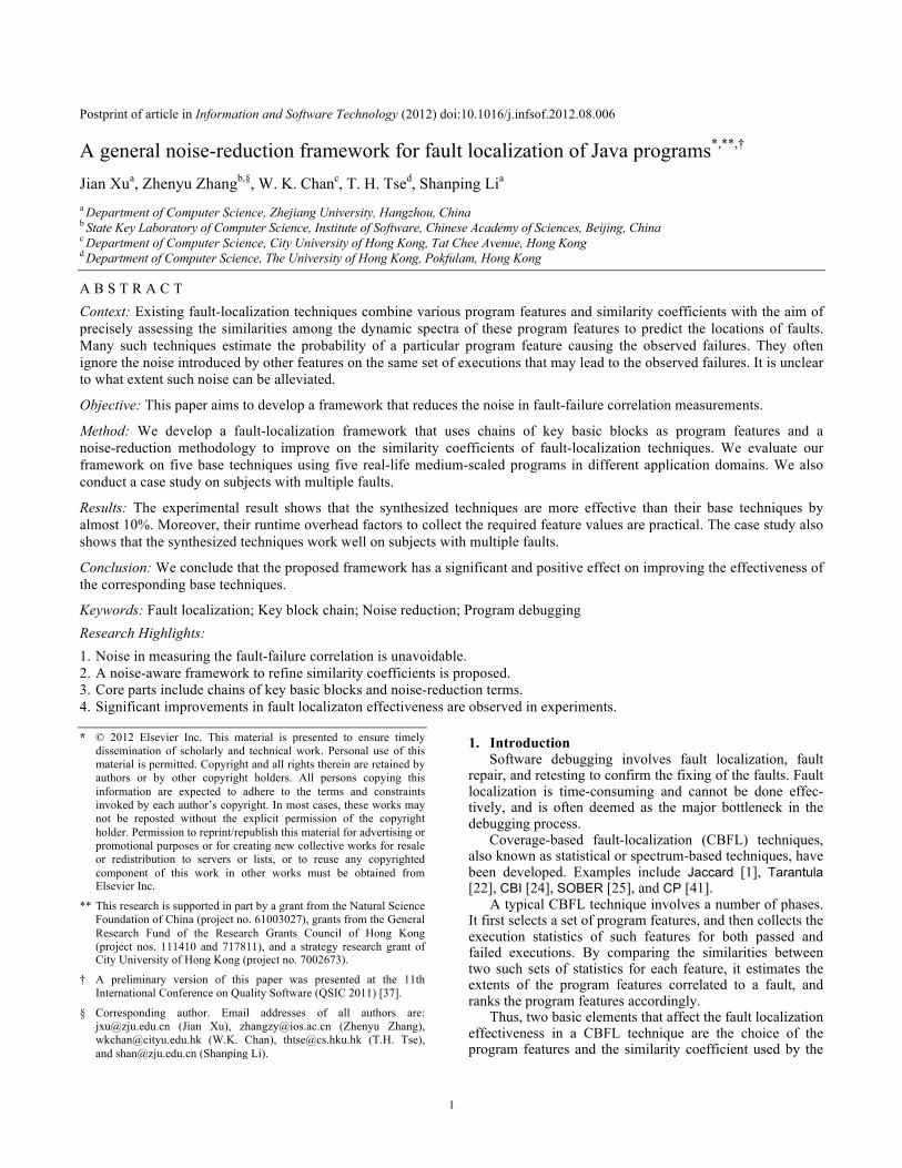
1

Postprint of article in Information and Software Technology (2012) doi:10.1016/j.infsof.2012.08.006

A general noise-reduction framework for fault localization of Java programs*,**,†

Jian Xua, Zhenyu Zhangb,§, W. K. Chanc, T. H. Tsed, Shanping Lia a Department of Computer Science, Zhejiang University, Hangzhou, China b State Key Laboratory of Computer Science, Institute of Software, Chinese Academy of Sciences, Beijing, China c Department of Computer Science, City University of Hong Kong, Tat Chee Avenue, Hong Kong d Department of Computer Science, The University of Hong Kong, Pokfulam, Hong Kong

A B S T R A C T Context: Existing fault-localization techniques combine various program features and similarity coefficients with the aim of precisely assessing the similarities among the dynamic spectra of these program features to predict the locations of faults. Many such techniques estimate the probability of a particular program feature causing the observed failures. They often ignore the noise introduced by other features on the same set of executions that may lead to the observed failures. It is unclear to what extent such noise can be alleviated.

Objective: This paper aims to develop a framework that reduces the noise in fault-failure correlation measurements.

Method: We develop a fault-localization framework that uses chains of key basic blocks as program features and a noise-reduction methodology to improve on the similarity coefficients of fault-localization techniques. We evaluate our framework on five base techniques using five real-life medium-scaled programs in different application domains. We also conduct a case study on subjects with multiple faults.

Results: The experimental result shows that the synthesized techniques are more effective than their base techniques by almost 10%. Moreover, their runtime overhead factors to collect the required feature values are practical. The case study also shows that the synthesized techniques work well on subjects with multiple faults.

Conclusion: We conclude that the proposed framework has a significant and positive effect on improving the effectiveness of the corresponding base techniques.

Keywords: Fault localization; Key block chain; Noise reduction; Program debugging Research Highlights: 1. Noise in measuring the fault-failure correlation is unavoidable. 2. A noise-aware framework to refine similarity coefficients is proposed. 3. Core parts include chains of key basic blocks and noise-reduction terms. 4. Significant improvements in fault localizaton effectiveness are observed in experiments.

1. Introduction Software debugging involves fault localization, fault

repair, and retesting to confirm the fixing of the faults. Fault localization is time-consuming and cannot be done effec-tively, and is often deemed as the major bottleneck in the debugging process.

Coverage-based fault-localization (CBFL) techniques, also known as statistical or spectrum-based techniques, have been developed. Examples include Jaccard [1], Tarantula [22], CBI [24], SOBER [25], and CP [41].

A typical CBFL technique involves a number of phases. It first selects a set of program features, and then collects the execution statistics of such features for both passed and failed executions. By comparing the similarities between two such sets of statistics for each feature, it estimates the extents of the program features correlated to a fault, and ranks the program features accordingly.

Thus, two basic elements that affect the fault localization effectiveness in a CBFL technique are the choice of the program features and the similarity coefficient used by the

* © 2012 Elsevier Inc. This material is presented to ensure timely dissemination of scholarly and technical work. Personal use of this material is permitted. Copyright and all rights therein are retained by authors or by other copyright holders. All persons copying this information are expected to adhere to the terms and constraints invoked by each author’s copyright. In most cases, these works may not be reposted without the explicit permission of the copyright holder. Permission to reprint/republish this material for advertising or promotional purposes or for creating new collective works for resale or redistribution to servers or lists, or to reuse any copyrighted component of this work in other works must be obtained from Elsevier Inc.

** This research is supported in part by a grant from the Natural Science Foundation of China (project no. 61003027), grants from the General Research Fund of the Research Grants Council of Hong Kong (project nos. 111410 and 717811), and a strategy research grant of City University of Hong Kong (project no. 7002673).

† A preliminary version of this paper was presented at the 11th International Conference on Quality Software (QSIC 2011) [37].

§ Corresponding author. Email addresses of all authors are: [email protected] (Jian Xu), [email protected] (Zhenyu Zhang), [email protected] (W.K. Chan), [email protected] (T.H. Tse), and [email protected] (Shanping Li).

Administrator

HKU CS Tech Report TR-2012-13

2

technique. Existing work has proposed many similarity coefficients

[1][4][24][25][30][39][41] or derived coefficients [31][45]. Many experiments have been conducted on these different coefficients under various benchmarks to compare their effectiveness. Nonetheless, for the same class of similarity coefficients, there is still no consensus on why one similar-ity coefficient is consistently better than others in the class. Existing literature uses empirical findings to validate the proposals, and yet their fault localization effectiveness on different program subjects often varies.

A CBFL technique abstractly models a program as a set of features, such as nodes [3][22], edges [31][41], predicates [24][25], sequences of edges [12], sequences of conditionals in predicates [5][44], and data values [18], and estimates the likelihood (such as fault suspiciousness) that each feature is related to the observed failures or anomalies. From the above list of proposals, we observe that finding a good set of features is obviously important.

Ideally, the source code of a program can be statically and completely partitioned into a set of equivalent classes of these features. For instance, basic blocks can be used as an equivalence criterion, in which case every statement in any basic block can be assigned to exactly one partition. Such a partitioning process may also be applied when statements, edges, and predicates, to name a few, are used as a feature.

Surprisingly, when a typical CBFL technique focuses on one partition A during the fault suspiciousness assessment process, it (or its coefficient similarity formula) consistently ignores other partitions in the same execution, and yet the failure verdict for partition A is in fact related to all the partitions along the same execution. For a long-lived execution, the noise introduced by such deliberately ignored partitions may exhibit a significant impact on the accuracy of the measured correlation value.

Our previous work [37] proposed the notion of noise reduction and proposed a technique Minus to reduce noise incurred in Tarantula. It showed that reducing the noise from unwanted features improves the effectiveness of Tarantula. It also proposed a feature known as KBC for fault localization, which intuitively means a chain of basic blocks, and showed via an empirical study that simultaneously applying both Minus and KBC can synthesize a more promising novel technique MKBC. Its experiment showed that MKBC was more effective than Tarantula, Jaccard, and Ochiai in locating faults in three medium-scaled program subjects.

Naish et al. [28] proposed a model for spectrum-based fault localization, in which four terms are used as arguments of the similarity coefficient formulas of 33 selected fault-localization techniques. For example, the similarity coefficient of Tarantula is:

𝑎!"

𝑎!" + 𝑎!"𝑎!"

𝑎!" + 𝑎!"+

𝑎!"𝑎!" + 𝑎!"

where aef means the number of failed executions covering a target program feature and anf means the number of failed

executions not covering it. The arguments aep and anp can be explained in the same way, except that they count the passed executions instead. In our previous work [37], we have shown that reducing the noise means subtracting the possibility of not executing a feature causing a failure, and proposed to exchange the executed and non-executed parts to estimate the noise [37]. In the same manner, we use anf instead of aef, anp instead of aep, aef instead of anf, and aep instead of anp to estimate the noise in Tarantula as follows:

𝑎!"𝑎!" + 𝑎!"

𝑎!"𝑎!" + 𝑎!"

+𝑎!"

𝑎!" + 𝑎!"

For each of the other 32 techniques, can we synthesize a new technique similarly? Will they also be effective?

In this paper, we generalize the concept of noise- reduction in MKBC to propose a general fault-localization framework that can be used to synthesize various fault- localization techniques based on the inputted existing tech-nique. We reproduce in the second column of Table V the synthesized formulas for all the 33 techniques in [28]. To verify the efficacy and efficiency of our framework, we significantly extend a controlled experiment reported in [37] by taking four more existing fault-localization techniques Jaccard [1], Ochiai [39], Ochiai2 [28], and Kulczynski2 [28] in addition to Tarantula [22] as inputs to synthesize new techniques and two more medium-scaled real-life programs jmeter and nanoxml in addition to jtopas, xmlsecurity, and ant as subject programs. Our framework benefits from the ideas of Minus and KBC proposed in our previous work [37] in figuring out the factors with significant effects. In this paper, we additionally investigate the effect of the synthe-sized techniques by applying Minus, KBC, or their combina-tion to an inputted based technique. We find empirically that applying either Minus or KBC separately, or applying both of them simultaneously, can synthesize a more effective technique from any base fault-localization technique over any program. We also investigate empirically the impacts of program failing rate and the length of a KBC on the effectiveness of the synthesized techniques, as well as their efficiency issues. The result shows that both the failing rate and the length of KBC can be significant factors. Finally, we report on a case study demonstrating that our methodology can effectively locate faults in a real-life program containing multiple faults.

The main contribution of this paper is twofold: (i) It proposes the first framework with a novel noise-reduction methodology to synthesize fault-localization techniques. (ii) It reports a controlled experiment that applies different base fault-localization techniques to different subject programs to verify that the synthesized techniques are consistently more effective than their base counterpart, which indicates that our proposed methodology and framework are promising.

The rest of this paper is organized as follows. Section 2 shows a motivating example. Section 3 presents our frame-work. Section 4 presents an experimental evaluation. Sec-tion 5 conducts a case study to further analyze the exper-imental results. Section 6 highlights some potential threats aaaaa

3

Java statements and Jimple statements Test cases t1 t2 t3 t4 t5 t6 t7 t8 t9 t10

Tarantula

TMinusFKBC

TKBC

TMinusF

Jaccard

JMinusF

Ochiai

OM

inusF

Pass/Fail F P F P P P P P P P sus r sus r sus r sus r sus r sus r sus r sus r if (isAbsolute) {

index = path.indexOf(File.separatorChar, 0); if (index == -1) { return path.substring(1) + ":[000000]"; } else { device = path.substring(1, index++); }} ...

if (!isAbsolute && directory != null) {

directory.trim();

directory.insert(0, '.'); }

s1 ■ ■ ■ ■ ■ ■ ■ ■ ■ ■ 0.5 6 0.44 4 0.8 4 0.5 3 0.2 6 0.2 4 0.447 5 0.447 3 s2 ■ ■ ■ ■ ■ ■ ■ ■ 0.57 5 0.44 4 0.8 4 0.57 2 0.25 5 0.25 2 0.5 4 0.5 2 s3 ■ ■ ■ ■ ■ ■ ■ ■ 0.57 5 0.44 4 0.8 4 0.57 2 0.25 5 0.25 2 0.5 4 0.5 2

s4 ■ ■ 0.8 1 0.44 4 0.8 4 0.44 4 0.33 1 0.219 3 0.5 4 0.25 4

s5 ■ ■ ■ ■ ■ ■ 0.44 7 –0.13 8 0.44 8 –0.13 7 0.17 7 0.027 7 0.289 8 –0.07 8

s6 ■ ■ ▲ ▲ ■ ▲ ■ ■ 0.36 8 0.27 7 0.67 7 –0.44 8 0.11 8 -0.22 8 0.5 4 0 7 s7 ■ ■ ■ 0.66 3 0.27 7 0.67 7 0.27 6 0.25 5 0.125 6 0.408 7 0.141 6

s8 ■ ■ ■ 0.66 3 0.27 7 0.67 7 0.27 6 0.25 5 0.125 6 0.408 7 0.141 6

code examination effort 62.5% 50% 50% 25% 62.5% 25% 62.5% 25%

Figure 1. A faulty version of program ant and effectiveness comparison of different fault localization techniques. Legend. sus: suspiciousness of a statement/block/path being related to a fault; r: ranking of a statement/block/path.

to validity. Section 7 discusses the extensibility of our framework. Section 8 reviews related work, followed by Section 9 that concludes the paper.

Motivating example This section uses an example to motivate the needs of a

noise-reduction framework for fault localization. Figure 1 shows the program code excerpted from a faulty version of the program ant, downloaded from the Software-artifact Infrastructure Repository (SIR) [14]. The functionality of this code excerpt is to translate the path of a file from OS-format into VM-format. A fault exists on statement S2, where the second parameter of method path.indexOf() should be 1 rather than 0. Exercising S2 followed by S4 triggers a failure.

2.1 Jimple Jimple is an intermediate representation [32][33] of Java,

which can be directly created based on Java source code and Java bytecode/Java class files. We only have to handle 15 Jimple instructions instead of more than 200 instructions in Java bytecode. In addition, Jimple has several desirable properties to support fault localization. First, Jimple always normalizes every compound Boolean expression into atomic Boolean expressions, each of which resides in exactly one basic block.1 Second, each basic block contains at most one atomic Boolean expression. Third, mapping a Boolean expression in Jimple code to its corresponding statement in Java code is easy.

The Jimple code of the program excerpt2 and the control

1 In particular, a Jimple if_stmt [33] is an atomic Boolean expression. In

this paper, we do not consider other branch statements such as goto_stmt, table_switch_stmt, and lookup_switch_stmt [33].

2 Note that, to realize the streamlined form [32][33] in Jimple, the source code has been transformed with some branches switched without altering the program behavior. For example, the condition “index == –1”

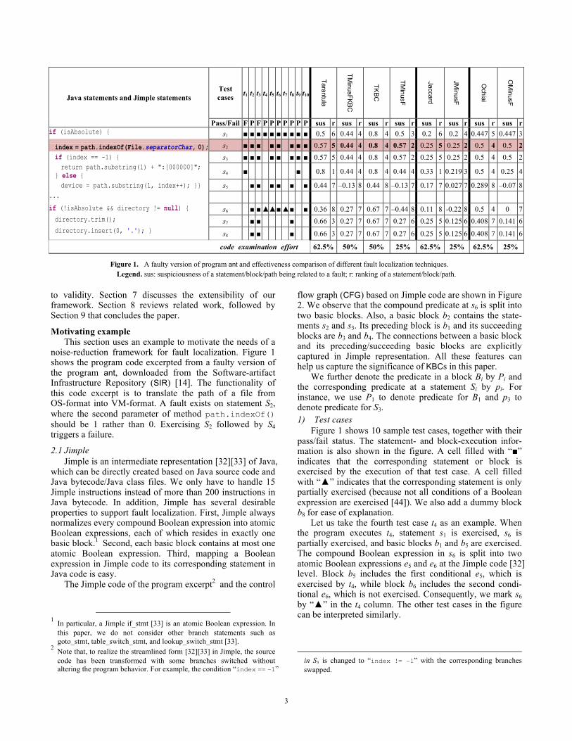
flow graph (CFG) based on Jimple code are shown in Figure 2. We observe that the compound predicate at s6 is split into two basic blocks. Also, a basic block b2 contains the state-ments s2 and s3. Its preceding block is b1 and its succeeding blocks are b3 and b4. The connections between a basic block and its preceding/succeeding basic blocks are explicitly captured in Jimple representation. All these features can help us capture the significance of KBCs in this paper.

We further denote the predicate in a block Bi by Pi and the corresponding predicate at a statement Si by pi. For instance, we use P1 to denote predicate for B1 and p3 to denote predicate for S3. 1) Test cases

Figure 1 shows 10 sample test cases, together with their pass/fail status. The statement- and block-execution infor-mation is also shown in the figure. A cell filled with “■” indicates that the corresponding statement or block is exercised by the execution of that test case. A cell filled with “▲” indicates that the corresponding statement is only partially exercised (because not all conditions of a Boolean expression are exercised [44]). We also add a dummy block b8 for ease of explanation.

Let us take the fourth test case t4 as an example. When the program executes t4, statement s1 is exercised, s6 is partially exercised, and basic blocks b1 and b5 are exercised. The compound Boolean expression in s6 is split into two atomic Boolean expressions e5 and e6 at the Jimple code [32] level. Block b5 includes the first conditional e5, which is exercised by t4, while block b6 includes the second condi-tional e6, which is not exercised. Consequently, we mark s6 by “▲” in the t4 column. The other test cases in the figure can be interpreted similarly.

in S3 is changed to “index != –1” with the corresponding branches swapped.

4

Java statements and Jimple statements Test cases t1 t2 t3 t4 t5 t6 t7 t8 t9 t10

CFG Pass/Fail F P F P P P P P P P

Block 1:[preds:] [succs: 2 5] ... e1: 1: if isAbsolute == 0 goto if isAbsolute!=0. Block 2:[preds: 1] [succs: 3 4] 2: $c0 = <java.io.File: char separatorChar> 2: index = virtualinvoke path.($c0, 0) e2: 3: if index != -1 goto index = index + 1 Block 3:[preds: 2] [succs:] ... 4: return $r3 Block 4:[preds: 2] [succs: 5] 5: index = index + 1 5: virtualinvoke path. ... Block 5:[preds: 1 4] [succs: 6 8] e5: 6: if isAbsolute != 0 goto return Block 6:[preds: 5] [succs: 7 8] e6: 6: if directory == null goto return Block 7:[preds: 6] [succs: 8] 7: virtualinvoke directory. ... 8：... Block 8:[preds: 5 6 7] [succs:] return

b1 ■ ■ ■ ■ ■ ■ ■ ■ ■ ■

b2 ■ ■ ■ ■ ■ ■ ■ ■

b3 ■ ■

b4 ■ ■ ■ ■ ■ ■

b5 ■ ■ ■ ■ ■ ■ ■ ■

b6 ■ ■ ■ ■ ■

b7 ■ ■ ■

b8

Figure 2. Jimple code and CFG for program excerpt in Figure 1.

2.2 Sample techniques We use the Jaccard, Ochiai, and Tarantula techniques to

demonstrate the idea of fault-localization framework, which synthesizes more effective new techniques from a given one. Let us take the technique Tarantula as example. We use the terms TMinusF, TKBC, and TMinusFKBC to stand for the techniques synthesized by separately and simultaneously applying the Minus and the KBC concepts, respectively. Further, we use JMinusF and OMinusF to stand for the synthesized techniques for Jaccard and Ochiai by using the Minus concept only. We apply the eight techniques to the example and compute, for each statement, a suspiciousness score and its rank. They are shown in the “sus” and “r” columns, respectively. By calculating the value of expense [41] for each technique, the effectiveness of these techniques in locating the fault in s2 is measured by the percentage of code that must be examined (as recommended by the expense) to include S2. The value of expense is shown in the “code examination effort” row.

2.3 Our idea Our idea of synthesizing a fault-localization technique

from a given one consists of three steps. First, a similarity coefficient is chosen from the base technique. Our frame-work then creates a new term according to the Minus concept to quantify the noise related to the given similarity coefficient.

Let us revisit the concepts of KBC and Minus to motivate the idea. To construct KBC, we traverse the Jimple code, block by block starting from b1, to search for a chain of adjacent blocks that end with a branch statement (which contains an atomic Boolean expression [44]). Because the last statement in b1 is a branch statement, we mark b1 and continue the traversal with b2. We also mark b2 because its last statement is again a branch statement. We then visit b3, which does not end with branch statement. Thus, we link the marked blocks b1 and b2 to form a key block chain (or KBC for short). In Figure 2, the thick (red) arrow from b1 to b2 denotes that they form a KBC. Note that b3 is not included. We then clear the marks and continue with the traversal to the next block, which is b4. Finally, we construct another KBC by linking b5 and b6, as shown by the dashed (blue) arrow. In short, we have two KBCs. The chains of atomic Boolean expressions (in the branch statements) are c1 = 〈e1, e2〉 and c2 = 〈e5, e6〉. We use the term KBC predicates to refer to such chains. In fact, the above process can be applied directly to Java code. We will give an example in Section 7.2.

A KBC predicate may contain several atomic Boolean expressions. We use them to construct sub-paths according to the evaluation sequences [44] of their decision results. Given a KBC ci, let esj(ci) denote the j-th sub-path of ci. In Figure 3, three sub-paths are constructed for each of the two KBCs c1 and c2, which will be our fault predicators here. Let us revisit the technique derived from Tarantula in our previous work [37] to inspire the idea in this paper.

b1

b4

b3

b2

b5

b6

b7

b8

5

KBC predicates for TKBC TMinusFKBC

c1 = 〈e1, e2〉 sus r sus r es1(c1) b1gb5 0 6 –0.57 6 es2(c1) b1gb2gb3 0.8 1 0.44 1 es3(c1) b1gb2gb4 0.44 3 –0.13 3

c2 = 〈e5, e6〉 sus r sus r es1(c2) b5gb8 0 6 –0.57 6 es2(c2) b5gb6gb8 0 6 –0.57 6 es3(c2) b5gb6gb7 0.67 2 0.27 2

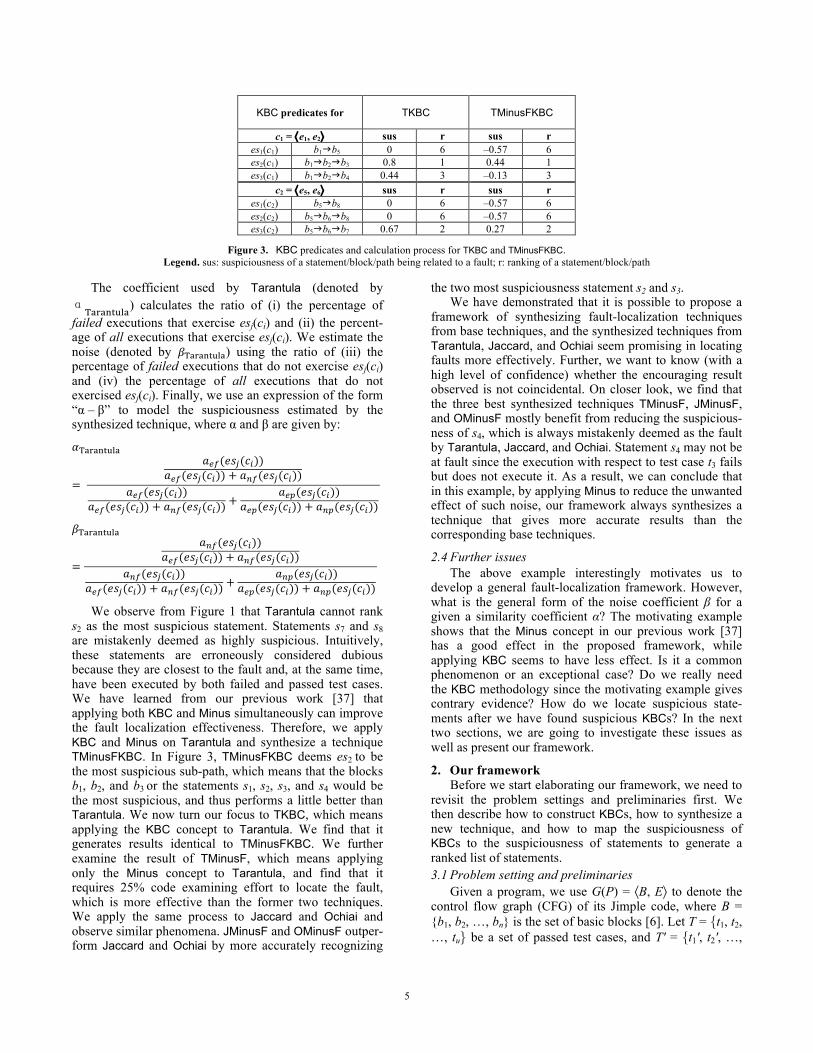
Figure 3. KBC predicates and calculation process for TKBC and TMinusFKBC. Legend. sus: suspiciousness of a statement/block/path being related to a fault; r: ranking of a statement/block/path

The coefficient used by Tarantula (denoted by

α!"#"$%&'") calculates the ratio of (i) the percentage of failed executions that exercise esj(ci) and (ii) the percent-age of all executions that exercise esj(ci). We estimate the noise (denoted by 𝛽!"#"$%&'") using the ratio of (iii) the percentage of failed executions that do not exercise esj(ci) and (iv) the percentage of all executions that do not exercised esj(ci). Finally, we use an expression of the form “α – β” to model the suspiciousness estimated by the synthesized technique, where α and β are given by:

𝛼!"#"$%&'"

=

𝑎!"(𝑒𝑠!(𝑐!))𝑎!"(𝑒𝑠!(𝑐!)) + 𝑎!"(𝑒𝑠!(𝑐!))

𝑎!"(𝑒𝑠!(𝑐!))𝑎!"(𝑒𝑠!(𝑐!)) + 𝑎!"(𝑒𝑠!(𝑐!))

+𝑎!"(𝑒𝑠!(𝑐!))

𝑎!"(𝑒𝑠!(𝑐!)) + 𝑎!"(𝑒𝑠!(𝑐!))

𝛽!"#"$%&'"

=

𝑎!!(𝑒𝑠!(𝑐!))𝑎!"(𝑒𝑠!(𝑐!)) + 𝑎!"(𝑒𝑠!(𝑐!))

𝑎!!(𝑒𝑠!(𝑐!))𝑎!"(𝑒𝑠!(𝑐!)) + 𝑎!"(𝑒𝑠!(𝑐!))

+𝑎!!(𝑒𝑠!(𝑐!))

𝑎!"(𝑒𝑠!(𝑐!)) + 𝑎!"(𝑒𝑠!(𝑐!))

We observe from Figure 1 that Tarantula cannot rank

s2 as the most suspicious statement. Statements s7 and s8 are mistakenly deemed as highly suspicious. Intuitively, these statements are erroneously considered dubious because they are closest to the fault and, at the same time, have been executed by both failed and passed test cases. We have learned from our previous work [37] that applying both KBC and Minus simultaneously can improve the fault localization effectiveness. Therefore, we apply KBC and Minus on Tarantula and synthesize a technique TMinusFKBC. In Figure 3, TMinusFKBC deems es2 to be the most suspicious sub-path, which means that the blocks b1, b2, and b3 or the statements s1, s2, s3, and s4 would be the most suspicious, and thus performs a little better than Tarantula. We now turn our focus to TKBC, which means applying the KBC concept to Tarantula. We find that it generates results identical to TMinusFKBC. We further examine the result of TMinusF, which means applying only the Minus concept to Tarantula, and find that it requires 25% code examining effort to locate the fault, which is more effective than the former two techniques. We apply the same process to Jaccard and Ochiai and observe similar phenomena. JMinusF and OMinusF outper-form Jaccard and Ochiai by more accurately recognizing

the two most suspiciousness statement s2 and s3. We have demonstrated that it is possible to propose a

framework of synthesizing fault-localization techniques from base techniques, and the synthesized techniques from Tarantula, Jaccard, and Ochiai seem promising in locating faults more effectively. Further, we want to know (with a high level of confidence) whether the encouraging result observed is not coincidental. On closer look, we find that the three best synthesized techniques TMinusF, JMinusF, and OMinusF mostly benefit from reducing the suspicious-ness of s4, which is always mistakenly deemed as the fault by Tarantula, Jaccard, and Ochiai. Statement s4 may not be at fault since the execution with respect to test case t3 fails but does not execute it. As a result, we can conclude that in this example, by applying Minus to reduce the unwanted effect of such noise, our framework always synthesizes a technique that gives more accurate results than the corresponding base techniques.

2.4 Further issues The above example interestingly motivates us to

develop a general fault-localization framework. However, what is the general form of the noise coefficient β for a given a similarity coefficient α? The motivating example shows that the Minus concept in our previous work [37] has a good effect in the proposed framework, while applying KBC seems to have less effect. Is it a common phenomenon or an exceptional case? Do we really need the KBC methodology since the motivating example gives contrary evidence? How do we locate suspicious state-ments after we have found suspicious KBCs? In the next two sections, we are going to investigate these issues as well as present our framework.

2. Our framework Before we start elaborating our framework, we need to

revisit the problem settings and preliminaries first. We then describe how to construct KBCs, how to synthesize a new technique, and how to map the suspiciousness of KBCs to the suspiciousness of statements to generate a ranked list of statements. 3.1 Problem setting and preliminaries

Given a program, we use G(P) = 〈B, E〉 to denote the control flow graph (CFG) of its Jimple code, where B = {b1, b2, …, bn} is the set of basic blocks [6]. Let T = {t1, t2, …, tu} be a set of passed test cases, and T' = {t1', t2', …,

6

tv'} be a set of failed test cases. Our aim is to find the most suspicious code that causes the observed failures.

3.2 MinusFKBC Framework Our framework consists of four major steps: the

identification of program features, the calculation of suspi-ciousness scores, and the mapping of the suspiciousness scores from Jimple blocks to Java statements, if necessary. In the first step, we assume the existence of a Jimple code parser so that we can work on the Jimple blocks to find KBC predicates and use them as program features. In the second step, we work on the collected execution data and calculate the suspiciousness score for each program feature. In the third step, we map the suspiciousness of identified program features to the suspiciousness of Jimple blocks. In the fourth step, if the mapping of Jimple code to Java code is not unique, we map the suspiciousness of Jimple code to Java statements. The four steps are illustrated in the over-view in Figure 4.

3.2.1 Constructing KBC predicates as program feature To construct KBCs, we traverse the Jimple [32][33]

code, block by block, starting from the first one. We in turn mark every block visited until we encounter a block whose last statement is not a branch statement. We link up all the marked blocks to form a section, and then clear all

the marks and continue with the traversal process. In such a way, we partition the Jimple code into a number of sections, and refer to each section as a Key Block Chain (KBC). In Figure 2, for example, we start from the first block b1 in the Jimple code, mark b1 and b2 in turn, find that b3 does not end with a branch statement, and thus construct a KBC n1.

Every KBC contains a sub-path for exercising blocks, each of which contains exactly one atomic predicate. The sub-path of atomic predicates in a KBC is called a KBC predicate. According to Jimple semantics, if such an atomic predicate in a block is evaluated to be true, the next adjacent block in the same KBC will not be executed, but the execution will jump to a succeeding block (defined by the “[succ]” annotation) of that block. For each KBC, by enumerating the possible underlying decision value of each atomic predicate, the corresponding KBC predicate can be mapped to a set of sub-paths in the program. We use the notation esj(ci) to denote the j-th sub-path with respect to the KBC ci. In Figure 3, for example, the KBC c1, which contains the atomic Boolean expressions e1 and e2, may be resolved into three sub-paths b1gb5, b1gb2gb3, and b1gb2gb4.

Suppose we use a Java program parser to obtain the list of Jimple blocks 𝐵 = 𝑏!, 𝑏!,… from the Java code excerpt. The resultant set of sub-paths 𝑃 = 𝑝!, 𝑝!,… is

Figure 4. Overview of our framework.

b4

s9 b7

p2

Sus(p1)

Sus(p2)

Sus(b7) Sus(s9)

2)

3) 4)

b1

b2

p1

1)

Java code Jimple code

successful test cases

failed test cases

t1 t2 t3 t4

3 5 3

2 6

7

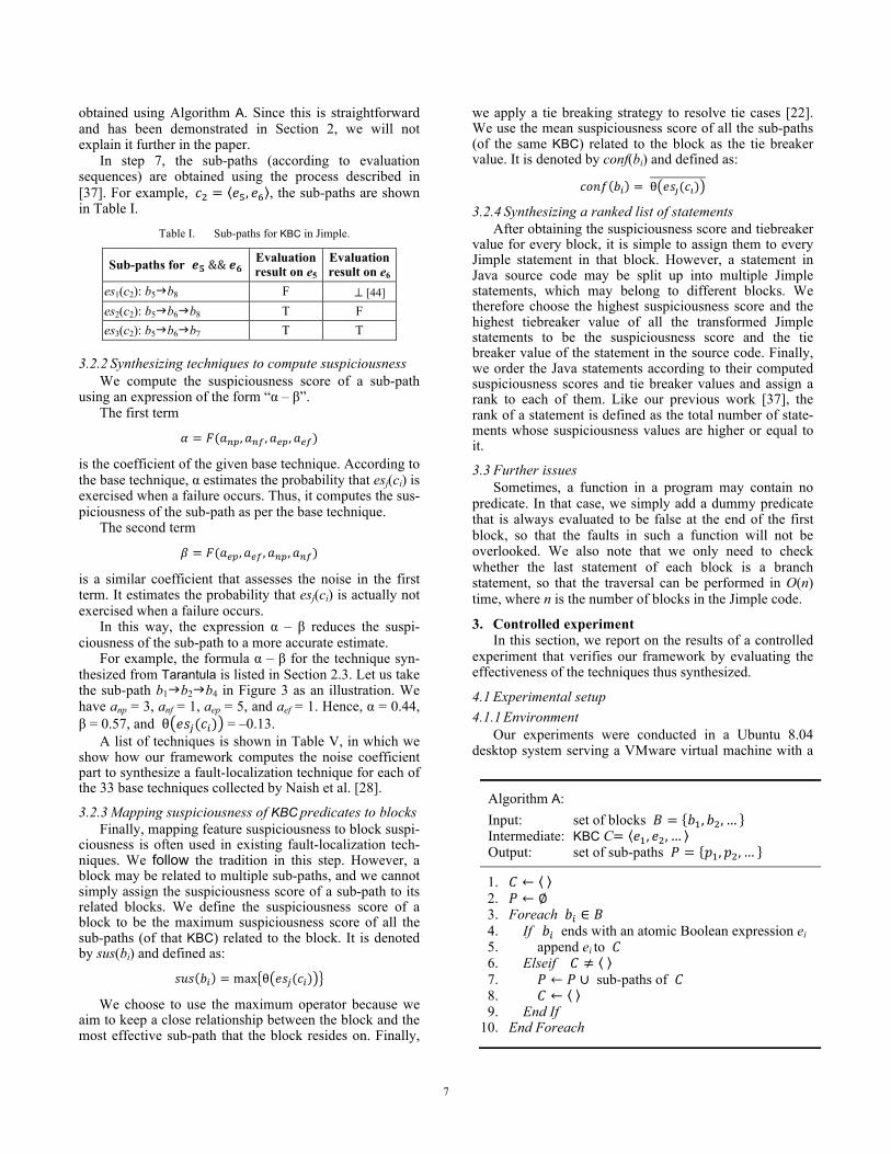
obtained using Algorithm A. Since this is straightforward and has been demonstrated in Section 2, we will not explain it further in the paper.

In step 7, the sub-paths (according to evaluation sequences) are obtained using the process described in [37]. For example, 𝑐! = 𝑒!, 𝑒! , the sub-paths are shown in Table I.

Table I. Sub-paths for KBC in Jimple.

Sub-paths for 𝒆𝟓 && 𝒆𝟔 Evaluation result on e5

Evaluation result on e6

es1(c2): b5gb8 F ⊥ [44] es2(c2): b5gb6gb8 T F es3(c2): b5gb6gb7 T T

3.2.2 Synthesizing techniques to compute suspiciousness We compute the suspiciousness score of a sub-path

using an expression of the form “α – β”. The first term

𝛼 = 𝐹(𝑎!", 𝑎!" , 𝑎!", 𝑎!")

is the coefficient of the given base technique. According to the base technique, α estimates the probability that esj(ci) is exercised when a failure occurs. Thus, it computes the sus-piciousness of the sub-path as per the base technique.

The second term

𝛽 = 𝐹(𝑎!", 𝑎!" , 𝑎!", 𝑎!") is a similar coefficient that assesses the noise in the first term. It estimates the probability that esj(ci) is actually not exercised when a failure occurs.

In this way, the expression α – β reduces the suspi-ciousness of the sub-path to a more accurate estimate.

For example, the formula α – β for the technique syn-thesized from Tarantula is listed in Section 2.3. Let us take the sub-path b1gb2gb4 in Figure 3 as an illustration. We have anp = 3, anf = 1, aep = 5, and aef = 1. Hence, α = 0.44, β = 0.57, and θ 𝑒𝑠!(𝑐!) = –0.13.

A list of techniques is shown in Table V, in which we show how our framework computes the noise coefficient part to synthesize a fault-localization technique for each of the 33 base techniques collected by Naish et al. [28].

3.2.3 Mapping suspiciousness of KBC predicates to blocks Finally, mapping feature suspiciousness to block suspi-

ciousness is often used in existing fault-localization tech-niques. We follow the tradition in this step. However, a block may be related to multiple sub-paths, and we cannot simply assign the suspiciousness score of a sub-path to its related blocks. We define the suspiciousness score of a block to be the maximum suspiciousness score of all the sub-paths (of that KBC) related to the block. It is denoted by sus(bi) and defined as:

𝑠𝑢𝑠 𝑏! = max θ 𝑒𝑠!(𝑐!)

We choose to use the maximum operator because we aim to keep a close relationship between the block and the most effective sub-path that the block resides on. Finally,

we apply a tie breaking strategy to resolve tie cases [22]. We use the mean suspiciousness score of all the sub-paths (of the same KBC) related to the block as the tie breaker value. It is denoted by conf(bi) and defined as:

𝑐𝑜𝑛𝑓 𝑏! = θ 𝑒𝑠!(𝑐!)

3.2.4 Synthesizing a ranked list of statements After obtaining the suspiciousness score and tiebreaker

value for every block, it is simple to assign them to every Jimple statement in that block. However, a statement in Java source code may be split up into multiple Jimple statements, which may belong to different blocks. We therefore choose the highest suspiciousness score and the highest tiebreaker value of all the transformed Jimple statements to be the suspiciousness score and the tie breaker value of the statement in the source code. Finally, we order the Java statements according to their computed suspiciousness scores and tie breaker values and assign a rank to each of them. Like our previous work [37], the rank of a statement is defined as the total number of state-ments whose suspiciousness values are higher or equal to it.

3.3 Further issues Sometimes, a function in a program may contain no

predicate. In that case, we simply add a dummy predicate that is always evaluated to be false at the end of the first block, so that the faults in such a function will not be overlooked. We also note that we only need to check whether the last statement of each block is a branch statement, so that the traversal can be performed in O(n) time, where n is the number of blocks in the Jimple code.

3. Controlled experiment In this section, we report on the results of a controlled

experiment that verifies our framework by evaluating the effectiveness of the techniques thus synthesized.

4.1 Experimental setup 4.1.1 Environment

Our experiments were conducted in a Ubuntu 8.04 desktop system serving a VMware virtual machine with a

Algorithm A:

Input: set of blocks 𝐵 = 𝑏!, 𝑏!,… Intermediate: KBC C= 𝑒!, 𝑒!,… Output: set of sub-paths 𝑃 = 𝑝!, 𝑝!,…

1. 𝐶 ← 2. 𝑃 ← ∅ 3. Foreach 𝑏! ∈ 𝐵 4. If 𝑏! ends with an atomic Boolean expression ei 5. append ei to 𝐶 6. Elseif 𝐶 ≠ 7. 𝑃 ← 𝑃 ∪ sub-paths of 𝐶 8. 𝐶 ← 9. End If

10. End Foreach

8

configuration of a single Intel® Core™ Duo 2.66 GHz CPU, and 512 MB memory. Our tool was developed on top of Soot version 2.3.0. All the programs and tools were compiled with JDK 1.6. Test cases were managed by the JUnit framework version 3. All the work was driven auto-matically using bash scripts.

4.1.2 Subject programs The controlled experiment used five medium-scaled

real-life programs, namely, jtopas, xmlsecurity, ant, jmeter, and nanoxml. We downloaded them (including all the faulty versions and associated test suites) from the SIR site [14]. Table II shows the descriptive statistics of each subject program, including the versions, the program size (in LOC), the number of faulty versions, and the size of the associated test pool. Following [22], we executed each version with each test case, and input the entire set of executions to each technique, which will be described below.

Following the documentation of SIR and the experi-mental process in previous work [1][24][41][44], we excluded the versions whose faults cannot be revealed by any test case. This is because both our techniques and peer techniques do comparisons on profiling produced by failed test cases and passed test cases. In addition, several old program versions such as ant versions prior to 1.6 (which were based on JDK 1.4) were excluded because our instrumentation tool, implemented on Soot version 2.3.0 running on JDK 1.6, does not support them. For nanoxml, we used the JUnit wrapper class test cases of its TSL test suite. These JUnit test cases are behaviorally equivalent to the TSL test suites provided with nanoxml. We finally used all the remaining 177 faulty versions in the experi-ment, as shown in Table II. 4.1.3 Base techniques

We chose five representative techniques from [28], namely Jaccard, Ochiai, Tarantula, Ochiai2, and Kulczynski2. We chose Tarantula because it is one of the earliest fault-localization techniques and has many variants [23][31][39]. It is representative of a family of variant techniques. We chose Jaccard and Ochiai because they are the two most effective fault-localization techniques reported in previous work [28][31][41]. We further chose the Ochiai2 technique. It is an enhancement of Ochiai and includes a noise-reduction part. We would like to know whether our noise-reduction proposal works compatibly

with it. Finally, we randomly picked Kulczynski2 from the remaining 29 techniques.

4.1.4 Synthesizing strategies We used each of the five techniques as base technique

to synthesize new fault-localization techniques. We used two synthesizing strategies: (i) Applying Minus or KBC separately to the 5 base techniques over 5 different pro-grams. (ii) Applying both Minus and KBC simultaneously to the 5 base techniques over 5 different programs. Thus, we can know the effects of Minus and KBC separately and evaluate the effect of their combination.

For the base technique Tarantula, we used the name TKBC for the synthesized technique that uses KBC as program features, TMinusF for the one that applies the Minus noise reduction in our framework, and TMinusFKBC for the one that applies both Minus and KBC simultane-ously. We named the techniques synthesized for the base techniques Jaccard and Ochiai in the same manner. To distinguish the Ochiai2 family from the Ochiai family, we added a number ‘2’ in the names for the former family. For example, when choosing Ochiai2 as the base technique, the three synthesized techniques were named as O2MinusF, O2KBC, and O2MinusKBC. The synthesized techniques for the base technique Kulczynski2 were similarly named. 4.1.5 Effectiveness metrics

Each of these techniques produces a ranked list of all the executed statements in descending order of their computed suspiciousness values. The rank of a statement is defined as the sum of the number of statements having higher suspiciousness scores and the number of statements sharing the same suspicious score.

Previous work [39] defined the expense metric as the ratio between the rank of the faulty statement and the total number of executable statements. We consider, however, that the use of the number of executed statements as the denominator in the expense formula is more suitable because other unrelated statements do not need to be checked in practice according to the PIE model [34]. We refer to this metric as the code examination effort.

If a fault is on a non-executable statement (such as a code omission fault), the use of dynamic execution information cannot help locate it directly. Following [18], we mark the directly affected statement or an adjacent executable statement as a fault position, followed by applying the expense metric.

Table II. Descriptive statistics of subject programs.

Real-Life versions Program description LOC No. of versions No. of test cases

jtopas 0.4 – 0.6 Text parser 5400 25 207

xmlsecurity 1.0.4 – 1.0.71 XML signature and encryption 16800 49 94

ant 1.6 beta Tool building 80500 22 830

jmeter 1.8 – 1.9 Performance test tool 43400 11 95

nanoxml 1.1–1.3,1.5 XML parser 7646 70 214

Total 177 1440

9

In the experiment, we inputted the entire test pool for each faulty version to each technique, and measured their expense values.

4.2 Effectiveness analysis 4.2.1 Overall effectiveness

Figure 5 shows the overall effectiveness of the tech-niques synthesized from our framework. The x-axis indi-cates the code examination effort, as explained Section 4.1.5. The y-axis indicates the percentage of faults located within the code examination effort indicated by the x- coordinate.

The curve with name X is generated by counting the faults located for all the 25 scenarios, that is, applying five different techniques to five different programs. For instance, by examining no more than 10 percent of the code in each of the 177 faulty versions, Jaccard locates faults in 27.68% of all the 177 faulty versions, while Ochiai, Tarantula, Ochiai2, and Kulczynski2 can locate faults in 27.68%, 24.86%, 9.61%, and 18.08% of all the 177 faulty versions, respectively. Thus, on average, a base technique can locate faults in (27.68% + 27.68% + 24.86% + 9.61% + 18.08%) / 5 = 21.58% in all the 177 faulty versions and hence the curve X passes through the point (10%, 21.58%). The curves XMinusF, XKBC, and XMinusFKBC, can be interpreted similarly.

We observe that the curves XMinusF and XKBC have consistent gaps above the curve X. It means that applying either Minus or KBC separately in our framework synthesizes a technique having better effectiveness than

the base technique. Further, we observe that the curve XMinusFKBC has consistent gaps above the curves XMinusF and XKBC. It means that applying Minus and KBC simultaneously in our framework is a better choice (in this analysis dimension).

Further, we also want to know the detailed information on the effectiveness of applying each of the five tech-niques to each of the five programs, and will analyze them in the next section.

4.2.2 Individual effectiveness Figure 6 shows the effectiveness of the five technique

families over the five different programs. To give a better presentation, we use a box-plot to show the effectiveness of each technique.

In each plot, we use four columns to show (from left) the effectiveness of the base technique, the synthesized technique by applying Minus, the synthesized technique by applying KBC, and the synthesized technique by simul-taneously applying Minus and KBC, respectively. For each column, the upper star shows the maximum code examina-tion effort of applying a technique to locate faults in each faulty version of the specific program, whereas the lower star shows the minimum code examination effort. The top of the box corresponds to the 75% percentile of the code examination efforts of applying a technique to locate faults in each faulty version of the specific program, whereas the bottom of the box corresponds to the 25% percentile. The cross in the box indicates the median value of the code aaaaa

Figure 5. Overall effectiveness.

0%

10%

20%

30%

40%

50%

60%

70%

80%

90%

100%

0% 10% 20% 30% 40% 50% 60% 70% 80% 90% 100%

% o

f fau

lts lo

cate

d

code examination effort

X XMinusF XKBC XMinusFKBC

10

code

exa

min

atio

n ef

fort

over jtopas over xmlsecurity over ant over jmeter over nanoxml

Figure 6. Individual effectiveness.

0% 20% 40% 60% 80%

100%

0% 20% 40% 60% 80%

100%

0% 20% 40% 60% 80%

100%

0% 20% 40% 60% 80%

100%

0% 20% 40% 60% 80%

100%

0% 20% 40% 60% 80%

100%

0% 20% 40% 60% 80%

100%

0% 20% 40% 60% 80%

100%

0% 20% 40% 60% 80%

100%

0% 20% 40% 60% 80%

100%

0% 20% 40% 60% 80%

100%

0% 20% 40% 60% 80%

100%

0% 20% 40% 60% 80%

100%

0% 20% 40% 60% 80%

100%

0% 20% 40% 60% 80%

100%

0% 20% 40% 60% 80%

100%

0% 20% 40% 60% 80%

100%

0% 20% 40% 60% 80%

100%

0% 20% 40% 60% 80%

100%

0% 20% 40% 60% 80%

100%

0% 20% 40% 60% 80%

100%

0% 20% 40% 60% 80%

100%

0% 20% 40% 60% 80%

100%

0% 20% 40% 60% 80%

100%

0% 20% 40% 60% 80%

100%

11

examination efforts of applying a technique to locate faults in each faulty version of the specific program.

Let us take the Jaccard technique over the jtopas program as an example (see the left-most column in the top-left plot). The lower star shows that Jaccard uses a minimum code examination effort of 0.99% to locate a fault in one of 24 faulty versions of jtopas. The upper star shows that for difficult faults in some versions, Jaccard has to examine 100% of the code to locate them. The bottom and top of the box shows that the 25% and 75% percentiles for the code examination efforts with respect to each of the 24 faulty versions are 4.82% and 79.73%, respectively. The cross in the box indicates that the median value of the code examination effort for the 24 faulty versions is 11.49%. The other plots can be interpreted similarly.

We observe that in most cases in our framework, applying Minus or KBC separately or applying both Minus and KBC simultaneously to any base technique synthesizes a technique with better fault localization effectiveness, regardless of the program under study. Further, applying both Minus and KBC simultaneously synthesizes a more promising technique than applying Minus or KBC sepa-rately. This confirms our previous observation on Figure 5.

However, we also observe opposite effects in some exceptional situations when applying Minus and KBC simultaneously. For example, when applying Minus and

KBC simultaneously to Ochiai2 over nanoxml, the fault localization effectiveness deteriorates. We suspect that such unexpected results could be due to test suites that are ineffective in revealing failures and program structures that confuse fault-localization techniques.

Nevertheless, in most cases, applying both Minus and KBC simultaneously to a base technique can synthesize a more promising technique than applying Minus or KBC separately. In the next sections, we will further investigate the effectiveness of the former.

4.2.3 Impacts of failing rate In this section, we investigate the effect of failing rate

on fault-localization techniques. We refer to the failing rate of a faulty version as the proportion of failed execu-tions among all executions,. This concept is formally defined in our previous work [20][21].

We collect the code examination effort for applying every technique to locate a fault in each faulty version. We perform curve fitting to study the impacts of failing rate on code examination effort. Figure 7 shows the impacts of failing rate on code examination effort using different techniques, whereas Figure 8 shows the impacts of failing rate on code examination effort for different programs. Our curve-fitting strategy is to try linear, logarithmic, polynomial, power, exponential, and moving average curves, and adopt the one (namely, line fitting) with the

code

exa

min

atio

n ef

fort

II.

JMinusFKBC OMinusFKBC TMinusFKBC O2MinusFKBC K2MinusFKBC

Figure 7. Impacts of failing rate on fault localization effectiveness for different techniques.

code

exa

min

atio

n ef

fort

jtopas xmlsecurity ant jmeter nanoxml

Figure 8. Impacts of failing rate on fault localization effectiveness for different programs.

0% 20% 40% 60% 80%

100%

0% 50% 100% failing rate

0% 20% 40% 60% 80%

100%


0% 20% 40% 60% 80%

100%


0% 20% 40% 60% 80%

100%


0% 20% 40% 60% 80%

100%


0% 20% 40% 60% 80%

100%


0% 20% 40% 60% 80%

100%


0% 20% 40% 60% 80%

100%


0% 20% 40% 60% 80%

100%


0% 20% 40% 60% 80%

100%


jtopas xmlsecurity

ant jmeter

nanoxml

jtopas xmlsecurity

ant jmeter

nanoxml

jtopas xmlsecurity

ant jmeter

nanoxml

jtopas xmlsecurity

ant jmeter

nanoxml

jtopas xmlsecurity

ant jmeter

nanoxml

JMinusFKBC OMinusFKBC TMinusFKBC

O2MinusFKBC K2MinusFKBC









12

least average fitting error. We believe that it will not only provide a good presentation but will better reflect the trends of the impacts under study.

We observe that for different techniques and different programs, failing rates always have negative impacts on fault localization effectiveness. In other words, the synthesized technique in our framework always needs to examine more code to locate faults with high failing rates. For example, the first plot of Figure 8 shows the impacts of failing rates on code examination effort using five different synthesized techniques over the jtopas program. The slopes for the lines are 0.2069, 0.204, 0.2026, 0.1721, and 0.2064 for JMinusFKBC, OMinusFKBC, TMinusFKBC, O2MinusFKBC, and K2MinusFBC, respectively. It roughly means that the ratio of the increasing speed of code examination effort and the increasing speed of the failing rate of faults is about 1:5 for different techniques over the jtopas program.

As a summary, we find that the techniques synthesized in our framework work better on faults with low failing rates. In practice, many faults are seldom exposed, and debuggers may be required to locate the fault in a program when only a small number of failed executions are availa-ble. If we deem the faults in more practical contexts to be faults with low failing rates, we can re-summarize our observation as “the techniques synthesized in our frame-

work work better in more practical scenarios”.

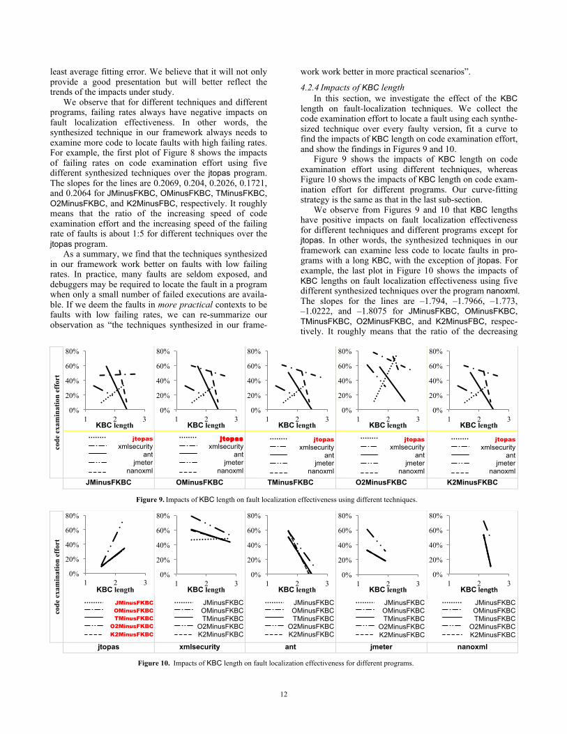
4.2.4 Impacts of KBC length In this section, we investigate the effect of the KBC

length on fault-localization techniques. We collect the code examination effort to locate a fault using each synthe-sized technique over every faulty version, fit a curve to find the impacts of KBC length on code examination effort, and show the findings in Figures 9 and 10.

Figure 9 shows the impacts of KBC length on code examination effort using different techniques, whereas Figure 10 shows the impacts of KBC length on code exam-ination effort for different programs. Our curve-fitting strategy is the same as that in the last sub-section.

We observe from Figures 9 and 10 that KBC lengths have positive impacts on fault localization effectiveness for different techniques and different programs except for jtopas. In other words, the synthesized techniques in our framework can examine less code to locate faults in pro-grams with a long KBC, with the exception of jtopas. For example, the last plot in Figure 10 shows the impacts of KBC lengths on fault localization effectiveness using five different synthesized techniques over the program nanoxml. The slopes for the lines are –1.794, –1.7966, –1.773, –1.0222, and –1.8075 for JMinusFKBC, OMinusFKBC, TMinusFKBC, O2MinusFKBC, and K2MinusFBC, respec-tively. It roughly means that the ratio of the decreasing

code

exa

min

atio

n ef

fort

JMinusFKBC OMinusFKBC TMinusFKBC O2MinusFKBC K2MinusFKBC

Figure 9. Impacts of KBC length on fault localization effectiveness using different techniques.

code

exa

min

atio

n ef

fort

jtopas xmlsecurity ant jmeter nanoxml

Figure 10. Impacts of KBC length on fault localization effectiveness for different programs.

0%

20%

40%

60%

80%

1 2 3 KBC length

0%

20%

40%

60%

80%

1 2 3 KBC length

0%

20%

40%

60%

80%

1 2 3 KBC length

0%

20%

40%

60%

80%

1 2 3 KBC length

0%

20%

40%

60%

80%

1 2 3 KBC length

0%

20%

40%

60%

80%

1 2 3 KBC length

0%

20%

40%

60%

80%

1 2 3 KBC length

0%

20%

40%

60%

80%

1 2 3 KBC length

0%

20%

40%

60%

80%

1 2 3 KBC length

0%

20%

40%

60%

80%

1 2 3 KBC length

jtopas xmlsecurity

ant jmeter

nanoxml

jtopas xmlsecurity

ant jmeter

nanoxml

jtopas xmlsecurity

ant jmeter

nanoxml

jtopas xmlsecurity

ant jmeter

nanoxml

jtopas xmlsecurity

ant jmeter

nanoxml










O2MinusFKBC

K2MinusFKBC

13

speed of code examination effort and the increasing speed of the KBC length of programs is about 2:1 for different techniques (except O2MinusFKBC) over the ant program. It also means that KBC length has less impact on the fault localization effectiveness of the O2MinusFKBC technique than on others.

Let us now focus on the jtopas issue. We refer to the jtopas lines in all the plots of Figure 9 and all the lines in the jtopas plot of Figure 10, that is, the ten lines with (red) bold labels. We find that jtopas behaves exceptionally when compared with other programs. On closer investiga-tion, we found the reasons. Three versions of jtopas are used in the experiment, as listed in Table II. They are jtopas versions 0.4, 0.5, and 0.6. Among them, only the result of jtopas 0.6 shows exceptional trends. We thus conclude that the unexpected phenomenon is due to jtopas 0.6. We check the average KBC lengths for jtopas versions 0.4, 0.5, and 0.6 and obtain the results 1.85, 1.86, and 2.17, respectively. We find considerable program structure changes from jtopas 0.5 to jtopas 0.6. The fault localiza-tion effectiveness achieved by different techniques on the two versions is not quite comparable. In particular, we find that one particular fault is consistently difficult to locate in jtopas 0.6 whereas the same fault can be more easily located in jtopas 0.5 and 0.4. If we exclude this problematic case, nine of the ten lines (except the use of O2MinusFKBC over the jtopas program) show consistent trends with the other lines and plots in Figures 9 and 10. Applying the same review to the other program subjects results in very marginal changes, since they do not suffer from similar problems due to an overhaul of the program structure.

Except for the jtopas issue, most plots in the two figures show consistent trends in the impacts of KBC lengths on fault localization effectiveness. It appears that when the KBC length increases, the KBC predicates can provide together more information to help locate faults. Longer KBCs maintain more sub-paths, which give more clues to program structures and executions, thus favoring fault localization.

Finally, we note that a KBC can be viewed as a program unit. A longer KBC indicates that the program has more branches, which implies that the program unit is of higher complexity (in terms of McCabe cyclomatic complexity [10]). In summary, we find that the techniques synthesized in our framework work better on programs of

higher complexity than others, which confirms the useful-ness of our proposal.

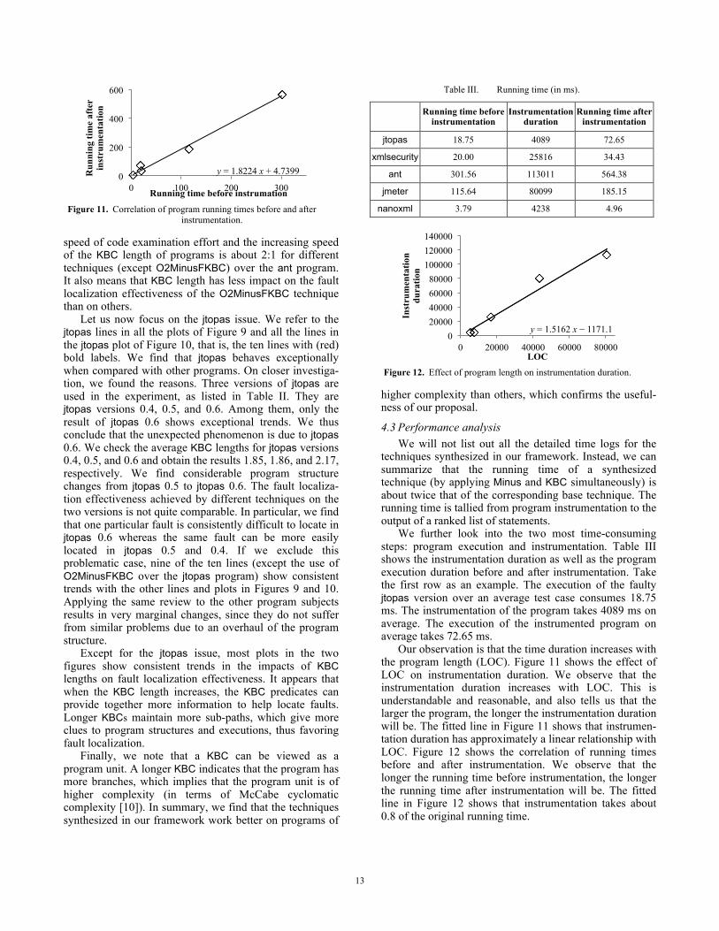
4.3 Performance analysis We will not list out all the detailed time logs for the

techniques synthesized in our framework. Instead, we can summarize that the running time of a synthesized technique (by applying Minus and KBC simultaneously) is about twice that of the corresponding base technique. The running time is tallied from program instrumentation to the output of a ranked list of statements.

We further look into the two most time-consuming steps: program execution and instrumentation. Table III shows the instrumentation duration as well as the program execution duration before and after instrumentation. Take the first row as an example. The execution of the faulty jtopas version over an average test case consumes 18.75 ms. The instrumentation of the program takes 4089 ms on average. The execution of the instrumented program on average takes 72.65 ms.

Our observation is that the time duration increases with the program length (LOC). Figure 11 shows the effect of LOC on instrumentation duration. We observe that the instrumentation duration increases with LOC. This is understandable and reasonable, and also tells us that the larger the program, the longer the instrumentation duration will be. The fitted line in Figure 11 shows that instrumen-tation duration has approximately a linear relationship with LOC. Figure 12 shows the correlation of running times before and after instrumentation. We observe that the longer the running time before instrumentation, the longer the running time after instrumentation will be. The fitted line in Figure 12 shows that instrumentation takes about 0.8 of the original running time.

Figure 11. Correlation of program running times before and after

instrumentation.

Table III. Running time (in ms).

Running time before instrumentation

Instrumentation duration

Running time after instrumentation

jtopas 18.75 4089 72.65

xmlsecurity 20.00 25816 34.43

ant 301.56 113011 564.38

jmeter 115.64 80099 185.15

nanoxml 3.79 4238 4.96

Figure 12. Effect of program length on instrumentation duration.

y = 1.8224 x + 4.7399 0

200

400

600

0 100 200 300

Run

ning

tim

e af

ter

inst

rum

enta

tion

Running time before instrumation

y = 1.5162 x − 1171.1 0

20000 40000 60000 80000

100000 120000 140000

0 20000 40000 60000 80000

Inst

rum

enta

tion

dura

tion

LOC

14

Considering Table III, Figure 11 and Figure 12, we conclude it is reasonable that the running time of the techniques synthesized in our framework increase with program scale and the techniques synthesized in our framework are applicable in practice.

4. Case study We used a case study to analyze the effectiveness of

our synthesized techniques in localizing faults in multi-fault program versions. We chose jtopas 0.4 as the program subject to evaluate the technique synthesized in our framework because we want to choose the most unfavorable subject to study and, according to the findings in the last sections, it happens to be jtopas. There are five faults in this release of jtopas, namely, FAULT_i for i = 1, 2, 5, 6, 10, as listed in Table IV.

In a multi-fault scenario, one fault may be the noise of another. We raise the following research question:

Q1: Does applying Minus and KBC simultaneously also synthesize a promising fault-localization technique for multi-fault programs?

We find that FAULT_1 and FAULT_2 are in the same class and the same method. Their locations are so close that both of them are trigged in most cases and one can hardly view them as two separate faults. FAULT_5 and FAULT_6 are in the same class but different methods. They have some impact on each other but are not tightly related. FAULT_10 is in a class different from the previous four.

The jtopas test cases are designed in a function- oriented manner. There are 8 test cases in total, each of which contains many test methods targeting at different functions of jtopas. For example, there are 24 methods in the test case de.susebox.TestExceptions.

During the execution of any test case, FAULT_10 or the combination of {FAULT_1, FAULT_2} seldom interacts

with the other faults. On the other hand, when executing a large number of test cases, FAULT_5 and FAULT_6 interact with each other. Because of the latter phenomenon, we decide to investigate the effectiveness of the synthesized techniques synthesized in locating FAULT_5 and FAULT_6, and their combination (that is, a 2-fault version with FAULT_5 and FAULT_6 enabled).

The synthesized technique based on Jaccard located FAULT_5 in its single-fault version with a rank of 6. At the same time, the technique located FAULT_6 in its single-fault with a rank of 74. For the 2-fault version with both FAULT_5 and FAULT_6 enabled, FAULT_5 is the dominant one and the technique deems the statement containing FAULT_5 to be more suspicious. As a result, during the suspiciousness assessment, the noise from the statement containing FAULT_6 was reduced. The state-ment containing FAULT_5 was still given a rank of 6 while the statement containing FAULT_6 was ranked 829. This further illustrates the idea behind Minus: It confirms the rank of the dominant faulty statement by reducing the noise from other faults and hence lowering their ranks in a multi-fault program.

Further, we applied all the techniques to all the 2-fault versions of jtopas 0.4, and found that the techniques synthesized in our framework always have an advantage over the base technique. The results are shown in Figure 13, which can be interpreted similarly to Figure 6. For example, we observe that by applying Minus and KBC simultaneously, the synthesized technique JMinusFKBC has a better fault localization effectiveness than its base technique Jaccard in terms of the code examination effort for the best cases (0.6% and 0.7% for JMinusFKBC and Jaccard, respectively) and the mean code examination effort (0.7% and 1.2% for JMinusFKBC and Jaccard, respectively). Similar phenomena can be observed for the other base techniques. As a result, we can summarize the study and answer Q1 as follows.

A1: We find that our methodology can be promising for medium-sized multi-fault programs.

5. Threats to validity 5.1 Construct validity

KBC is a chain of basic blocks. After locating the most suspicious KBCs, we proceed to map the suspiciousness of KBCs to those of statements for consistency with the conventional output format of fault-localization techniques. Directly evaluating the suspicious KBCs may result in different observations and conclusions.

Table IV. Statistics of faults in jtopas 0.4

Fault Package Class Method Lines

FAULT_1 de.susebox.java.io de.susebox.java.io.ExtIOException ExtIOException(…) 43, 50

FAULT_2 de.susebox.java.io de.susebox.java.io.ExtIOException ExtIOException(…) 52, 58

FAULT_5 de.susebox.java.util de.susebox.java.util.AbstractTokenizer isKeyword(…) 773, 783

FAULT_6 de.susebox.java.util de.susebox.java.util.AbstractTokenizer test4Normal(…) 921

FAULT_10 de.susebox.java.lang de.susebox.java.lang.ExtIndexOutOfBoundsException ExtIndexOutOfBoundsException(..) 43, 49

Figure 13. Result on the 2-fault versions of jtopas 0.4.

0.00% 0.50% 1.00% 1.50% 2.00% 2.50% 3.00% 3.50%

code

exa

min

atio

n ef

fort

15

Using code examining effort as a metric in the experiment may cause threats to the construct validity of the results. This has also been reported in previous projects [41][44][45]. However, we are not aware of other popular metrics for evaluating the fault localization effectiveness.

To evaluate our methodology, we compare the effec-tiveness of a base technique on a given faulty version with the effectiveness of a corresponding technique synthesized using our framework. Such a comparison may not be proper in the following cases: (i) A faulty statement is executed in all failed runs but in very limited number of (or even no) passed runs. Many techniques such as Tarantula are optimal in locating such a fault, by assigning it a very high suspiciousness score (e.g., close to 1) and needs very low code examination effort (e.g., close to 0%) to locate it. In such a case, there is nearly no space for enhancement and the effectiveness of our methodology can hardly be shown. (ii) The faulty statement is in a basic block that is always executed (such as in the main entry), and none of the techniques can effectively locate it. In such a case, the effectiveness of our methodology cannot be easily observed. Including these problematic faulty versions as experiment subjects may have unexpected impacts on the empirical results and draw divergent conclusions. For example, one particular fault in the program jtopas 0.6 cannot be located until 100% of the code has been examined. As a result, Figures 9 and 10 in Section 4.2.4 show that KBC length has positive impacts on the fault localization effectiveness of the synthesized XMinusFKBC techniques. Their observed trends are not consistent with those of the other programs. We have discussed this issue in detail in Section 4.2.4.

5.2 Internal validity Soot 2.3.0 is based on Java 1.5 or higher, but some of

our subject programs were originally based on Java 1.4. We need to modify these subjects so that they are compati-ble to Java 1.5 or higher. For example, enum can be used as a program variable in Java 1.4 but is a keyword in Java 1.5. We have carefully reviewed the conversion.

We use Soot to insert probes into the Java bytecode. Soot gives a good solution for specific Java features such as exception handling. Previous work [17][40] has investi-gated this topic, as exception information in run time contains plenty of error information, thus providing good support to fault localization. In this paper, we consider exception handling in programs as normal control flow because Soot can transform a Java program into Jimple code and still maintain the exception handling structures. Hence, if faults are located in these “catch” blocks, the approach in this paper can still find them.

We have carefully assured that our tool in the experi-ment is reliable.

5.3 External validity Using other programs and faulty versions in the experi-

ment may produce different results. The strategy we used to construct a KBC is only one

possible solution among many. Other strategies are also

feasible. We briefly discuss some possible extensions of our work. The first strategy is to identify blocks containing predicates that are as long as possible. This strategy is close to the full path tracking idea used in HOLMES [12]. Such a strategy, however, requires a search of the longest path from a graph, which takes more than O(n) time. A second strategy is to identify blocks containing predicates and use a random sub-path of blocks to construct a chain. Yet another strategy is to identify sub-paths of blocks within certain lengths and split a long chain into several shorter ones. An optimal length of a block chain is hard to determine. Moreover, one limitation of the last two strategies is that they may link irrelevant blocks together.

Another important prospect is that KBC can be applied to any program entity level. In computing, compilers usually decompose programs into basic blocks as the first step in the analysis process. Other languages can also have streamline representations like Jimple for Java. We believe that applying KBC helps locate faults in these programs, but more experiments are needed to confirm it.

6. Further discussions 6.1 Can we use other techniques? In this paper, we use Minus to reduce noise for selected fault-localization techniques. We do not limit the use of other CBFL techniques, as far as they use similarity coefficients and belong to the same family of technique. KBC is considered as a fault predicator based on coverage profiling. It can be used in many other techniques that make use of coverage information, such as HOLMES, CP, and CBI. For example, CP calculates the suspiciousness of edges and captures the propagation of infected states via edges. It is straightforward to assess the suspiciousness of KBCs and capture the propagation of infected states via different KBCs. HOLMES uses path as the unit to assess the fault relevance. Feng and Gupta [16] made use of Bayesian networks to facilitate fault localization and did not limit the use of different types of program elements. Jeffrey et al. proposed Value Replacement [18], which alters variable values in statements to look for candidates whose variable states can turn failed runs into passed runs. KBC, as a kind of program element, can be used to drive them. For example, we may alter variable values in KBCs to search for a suspicious KBC.

In Table V, we list out how our framework synthesizes techniques for the 33 base techniques presented in [28]. Let us take the last one as example. For the technique Rogot2, the similarity coefficient is

𝛼!"#"$% =14

𝑎!"𝑎!" + 𝑎!"

+𝑎!"

𝑎!" + 𝑎!"+

𝑎!"𝑎!" + 𝑎!"

+𝑎!"

𝑎!" + 𝑎!"

Accordingly, following our model, the noise coefficient is:

𝛽!"#"$% =14

𝑎!"𝑎!" + 𝑎!"

+𝑎!"

𝑎!" + 𝑎!"+

𝑎!"𝑎!" + 𝑎!"

+𝑎!"

𝑎!" + 𝑎!"

As a result, RMinusFKBC uses the following coefficient:

16

Table V. The 33 statement-level fault-localization techniques and their noise coefficient formulas.

Name Similarity coefficient of the base technique (α ) Noise coefficient for the synthesized technique (β )

Jaccard 𝑎!"

𝑎!" + 𝑎!" + 𝑎!"

𝑎!"𝑎!" + 𝑎!" + 𝑎!"

Anderberg 𝑎!"

𝑎!" + 2(𝑎!" + 𝑎!")

𝑎!"𝑎!" + 2(𝑎!" + 𝑎!")

Sørensen-Dice 2𝑎!"

2𝑎!" + 𝑎!" + 𝑎!"

2𝑎!"2𝑎!" + 𝑎!" + 𝑎!"

Dice 2𝑎!"

𝑎!" + 𝑎!" + 𝑎!"

2𝑎!"𝑎!" + 𝑎!" + 𝑎!"

Kulczynski1 𝑎!"

𝑎!" + 𝑎!"

𝑎!"𝑎!" + 𝑎!"

Kulczynski2 12

𝑎!"𝑎!" + 𝑎!"

+𝑎!"

𝑎!" + 𝑎!"

12

𝑎!"𝑎!" + 𝑎!"

+𝑎!"

𝑎!" + 𝑎!"

Russell and Rao

𝑎!"𝑎!" + 𝑎!" + 𝑎!" + 𝑎!"

𝑎!"

𝑎!" + 𝑎!" + 𝑎!" + 𝑎!"

Hamann 𝑎!" + 𝑎!" − 𝑎!" − 𝑎!"𝑎!" + 𝑎!" + 𝑎!" + 𝑎!"

𝑎!" + 𝑎!" − 𝑎!" − 𝑎!"𝑎!" + 𝑎!" + 𝑎!" + 𝑎!"

Simple Matching

𝑎!" + 𝑎!"𝑎!" + 𝑎!" + 𝑎!" + 𝑎!"

𝑎!" + 𝑎!"

𝑎!" + 𝑎!" + 𝑎!" + 𝑎!"

Soka 2(𝑎!" + 𝑎!")

2(𝑎!" + 𝑎!") + 𝑎!" + 𝑎!"

2(𝑎!" + 𝑎!")2(𝑎!" + 𝑎!") + 𝑎!" + 𝑎!"

M1 𝑎!" + 𝑎!"𝑎!" + 𝑎!"

𝑎!" + 𝑎!"𝑎!" + 𝑎!"

M2 𝑎!"

𝑎!" + 𝑎!" + 2(𝑎!" + 𝑎!")

𝑎!"𝑎!" + 𝑎!" + 2(𝑎!" + 𝑎!")

Rogers & Tanimoto

𝑎!" + 𝑎!"𝑎!" + 𝑎!" + 2(𝑎!" + 𝑎!")

𝑎!" + 𝑎!"

𝑎!" + 𝑎!" + 2(𝑎!" + 𝑎!")

Goodman 2𝑎!" − 𝑎!" − 𝑎!"2𝑎!" + 𝑎!" + 𝑎!"

2𝑎!" − 𝑎!" − 𝑎!"2𝑎!" + 𝑎!" + 𝑎!"

Hamming 𝑎!" + 𝑎!" 𝑎!" + 𝑎!"

Euclid 𝑎!" + 𝑎!" 𝑎!" + 𝑎!"

17

Ochiai 𝑎!"

𝑎!" + 𝑎!" (𝑎!" + 𝑎!")

𝑎!"

𝑎!" + 𝑎!" (𝑎!" + 𝑎!")

Overlap 𝑎!"

𝑚𝑖𝑛 (𝑎!" , 𝑎!" , 𝑎!")

𝑎!"𝑚𝑖𝑛 (𝑎!" , 𝑎!" , 𝑎!")

Tarantula

𝑎!"𝑎!" + 𝑎!"

𝑎!"𝑎!" + 𝑎!"

+𝑎!"

𝑎!" + 𝑎!"

𝑎!"𝑎!" + 𝑎!"

𝑎!"𝑎!" + 𝑎!"

+𝑎!"

𝑎!" + 𝑎!"

Zoltar 𝑎!"

𝑎!" + 𝑎!" + 𝑎!" +10000𝑎!"𝑎!"

𝑎!"

𝑎!"

𝑎!" + 𝑎!" + 𝑎!" +10000𝑎!"𝑎!"

𝑎!"

Ample 𝑎!"

𝑎!" + 𝑎!"−

𝑎!"𝑎!" + 𝑎!"

𝑎!"

𝑎!" + 𝑎!"−

𝑎!"𝑎!" + 𝑎!"

Wong1 𝑎!" 𝑎!"

Wong2 𝑎!" − 𝑎!" 𝑎!" − 𝑎!"

Wong3 𝑎!" − 𝑎!" if 𝑎!" ≤ 22 + 0.1 𝑎!" − 2 if 2 < 𝑎!" ≤ 102.8 + 0.001 𝑎!" − 10 if 𝑎!" > 10

𝑎!" − 𝑎!" if 𝑎!" ≤ 22 + 0.1 𝑎!" − 2 if 2 < 𝑎!" ≤ 102.8 + 0.001 𝑎!" − 10 if 𝑎!" > 10

Ochiai2 𝑎!"𝑎!"

𝑎!" + 𝑎!" (𝑎!" + 𝑎!") 𝑎!" + 𝑎!" (𝑎!" + 𝑎!")

𝑎!"𝑎!"

𝑎!" + 𝑎!" (𝑎!" + 𝑎!") 𝑎!" + 𝑎!" (𝑎!! + 𝑎!")

Geometric Mean

𝑎!"𝑎!" − 𝑎!"𝑎!"

𝑎!" + 𝑎!" (𝑎!" + 𝑎!") 𝑎!" + 𝑎!" (𝑎!" + 𝑎!")

𝑎!"𝑎!" − 𝑎!"𝑎!"

𝑎!" + 𝑎!" (𝑎!" + 𝑎!") 𝑎!" + 𝑎!" (𝑎!" + 𝑎!")

Harmonic Mean

𝑎!"𝑎!" − 𝑎!"𝑎!" 𝑎!" + 𝑎!" 𝑎!" + 𝑎!" 𝑎!" + 𝑎!" 𝑎!" + 𝑎!" 𝑎!" + 𝑎!" 𝑎!" + 𝑎!"

+𝑎!"𝑎!" − 𝑎!"𝑎!! (𝑎!" + 𝑎!" )(𝑎!" + 𝑎!")

𝑎!" + 𝑎!" 𝑎!" + 𝑎!" 𝑎!" + 𝑎!" 𝑎!" + 𝑎!"

𝑎!"𝑎!" − 𝑎!"𝑎!" 𝑎!" + 𝑎!" 𝑎!" + 𝑎!" 𝑎!" + 𝑎!" 𝑎!" + 𝑎!" 𝑎!" + 𝑎!" 𝑎!" + 𝑎!"

+𝑎!"𝑎!" − 𝑎!"𝑎!" (𝑎!" + 𝑎!" )(𝑎!" + 𝑎!")

𝑎!" + 𝑎!" 𝑎!" + 𝑎!" 𝑎!" + 𝑎!" 𝑎!" + 𝑎!"

Arithmetic Mean

2𝑎!" 𝑎!" − 2𝑎!" 𝑎!"(𝑎!" + 𝑎!")(𝑎!" + 𝑎!" ) + (𝑎!" + 𝑎!" )(𝑎!" + 𝑎!")

2𝑎!" 𝑎!" − 2𝑎!" 𝑎!"

(𝑎!" + 𝑎!")(𝑎!" + 𝑎!" ) + (𝑎!" + 𝑎!" )(𝑎!" + 𝑎!")

Cohen 2𝑎!" 𝑎!" − 2𝑎!" 𝑎!"

(𝑎!" + 𝑎!")(𝑎!" + 𝑎!" ) + (𝑎!" + 𝑎!" )(𝑎!" + 𝑎!")

2𝑎!" 𝑎!" − 2𝑎!" 𝑎!"(𝑎!" + 𝑎!")(𝑎!" + 𝑎!" ) + (𝑎!" + 𝑎!" )(𝑎!" + 𝑎!")

Scott 4𝑎!"𝑎!" − 4𝑎!"𝑎!" − (𝑎!" − 𝑎!")!

(2𝑎!" + 𝑎!" + 𝑎!")(2𝑎!" + 𝑎!" + 𝑎!")

4𝑎!"𝑎!" − 4𝑎!"𝑎!" − (𝑎!" − 𝑎!")!

(2𝑎!" + 𝑎!" + 𝑎!")(2𝑎!" + 𝑎!" + 𝑎!")

Fleiss 4𝑎!"𝑎!" − 4𝑎!"𝑎!" − (𝑎!" − 𝑎!")!

2𝑎!" + 𝑎!" + 𝑎!" + (2𝑎!" + 𝑎!" + 𝑎!")

4𝑎!"𝑎!" − 4𝑎!"𝑎!" − (𝑎!" − 𝑎!")!

2𝑎!" + 𝑎!" + 𝑎!" + (2𝑎!" + 𝑎!" + 𝑎!")

Rogot1 12

𝑎!"2𝑎!" + 𝑎!" + 𝑎!"

+𝑎!"

2𝑎!" + 𝑎!" + 𝑎!"

12

𝑎!"2𝑎!" + 𝑎!" + 𝑎!"

+𝑎!"

2𝑎!" + 𝑎!" + 𝑎!"

Rogot2 14

𝑎!"𝑎!" + 𝑎!"

+𝑎!"

𝑎!" + 𝑎!"+

𝑎!"𝑎!" + 𝑎!"

+𝑎!"

𝑎!" + 𝑎!"

14

𝑎!"𝑎!" + 𝑎!"

+𝑎!"

𝑎!" + 𝑎!"+

𝑎!"𝑎!" + 𝑎!"

+𝑎!!

𝑎!" + 𝑎!"

18

θ 𝑒𝑠!(𝑐!) =14

𝑎!"𝑎!" + 𝑎!"

+𝑎!"

𝑎!" + 𝑎!"+

𝑎!"𝑎!" + 𝑎!"

+𝑎!"

𝑎!" + 𝑎!"

−14

𝑎!"𝑎!" + 𝑎!"

+𝑎!"

𝑎!" + 𝑎!"+

𝑎!"𝑎!" + 𝑎!"

+𝑎!"

𝑎!" + 𝑎!"

Definitely, there are many approaches to fault locali-

zation and approaches to enhancing fault localization effectiveness that do not belong to the discussed problem settings. For example, Zhang et al. [43] shortened dynamic slices to enhance fault localization. We are also interested in the result of integrating these techniques with our methodology. For instance, when pruning slices with confidence, the suspiciousness region related to KBCs are also reduced. However, how to integrate with such tech-niques is beyond the scope of this paper.

6.2 Can KBC live without Jimple? Jimple is a powerful intermediate representation of

Java programs. Programmers (including ourselves) use Jimple to easily instrument target programs, construct control flow graphs, and build KBCs. However, the main idea of KBC is independent with Jimple.

For instance, let us focus on the motivating example in Figure 14, which shows a Java code excerpt. To construct KBC from such Java code, we traverse block by block starting from b1 to search for a chain of adjacent blocks that end with a branch statement (containing a Boolean expression). Because the last statement in b1 is a branch statement, we mark b1 and continue with the traversal of b2. We also mark b2 because its last statement is again a branch statement. We then visit b3, which does not end with a branch statement. Thus, we link up the marked blocks b1 and b2 to form a KBC. We then clear the marks and continue with the traversal of the next block b4. The traversal stops again since we encounter a block that ends with a non-branch statement. We continue from b5 and finally construct another KBC for b5. We therefore obtain two KBCs. The chains of Boolean expressions (in the branch statements) are c1 = 〈e1, e2〉 and c2 = 〈e'5〉. Note that

we use e'5 to refer to the compound Boolean expression in statement s6 of the Java code in Figure 1. The generated KBC predicates and sub-paths are shown in Tables VI and VII.

Basically, KBCs can be generated from any representation of a control flow graph for any program, because the algorithm in Section 3.2.1 does not limit the type of code from which the set of blocks are generated and inputted to the algorithm.

6.3 Can the sub-paths generated from the KBC construction process be covered by a DC-, CC- or MC/DC-satisfied test suite? Sub-paths are generated during the KBC generation

process. Let us explain how we generate legitimate sub-paths. We recall that we first divide the code into KBCs and then generate sub-paths for the predicates included in each KBC. In the former step, the generation of KBCs misses no predicate, because only blocks ending with non-branch statements are excluded. In the latter step, the generation of sub-paths from the KBC predicates is an evaluation sequence analysis [44] and no legitimate sub-path is missed. As a result, the proposed generation process will produce all the sub-paths, so that the genera-tion can be regarded as a coverage criterion in terms of sub-paths. We next analyze the strengths of different coverage criteria, including decision coverage (DC), condition coverage (CC), modified condition/decision coverage (MC/DC), sub-path coverage, and path coverage.

When applied to Java code, a sub-path can be related to predicates from multiple branch statements. (For instance, es2(c1) in the previous section is related to the predicates e1 and e2 from statements s1 and s2, respectively.) As a result, the granularity of sub-paths is finer than the branches used in branch coverage analysis. We know that decision cover-age can be subsumed by sub-path coverage. On the other hand, a sub-path may be related to predicates not from branch statements. (For example, es2(c1) in Section 7.2 is not related to the predicate e'5 from statements s5.) As a result, the granularity of sub-paths is coarser than the paths used in path coverage analysis. In fact, path coverage subsumes sub-path coverage. There is no direct relation between CC and sub-path coverage, or between MC/DC and sub-path coverage. This is because CC and MC/DC separately look into each individual compound Boolean

b1: if isAbsolute != 0 goto b5

b2: index = virtualinvoke path. ... if index != -1 goto b4

b3: return $r3 b4: index = index + 1

device = virtualinvoke path. ... b5: if isAbsolute || directory == null

goto b7 b6: virtualinvoke directory. ...

virtualinvoke directory. ...

b7:

Figure 14. Demonstration of constructing KBCs from Java code.

Table VI. Sub-path for KBC in source code.

Sub-paths for c1 = 〈e1, e2〉 Evaluation result on e1

Evaluation result on e2

es1(c1): b1gb5 F ⊥ [44] es2(c1): b1gb2gb3 T T es3(c1): b1gb2gb4 T F

Table VII. Sub-path for KBC in source code

Sub-paths for c2 = 〈e'5〉 Evaluation result on e'5 es1(c2): b5gb7 T es2(c2): b5gb6 F

19

expression and aim at covering different combinations of their condition values, whereas sub-path coverage (under the KBC construction process) investigates multiple Bool-ean expressions to cover the combinations of their decision values.

When applied to Jimple code, when Jimple predicates are mapped back to the original Java code for some reason, things can be a little complicated. A compound Boolean expression in Java code will always be broken down into multiple atomic Boolean expressions, so there is an M:1 relationship in the mapping of Jimple predicates to Java predicates. According to the Jimple specification [32][33], multiple atomic Boolean expressions (broken down from a compound Boolean expression in Java code) will always form a sequence of blocks, all of which will end with a predicate statement. As a result, for each compound Boolean expression in Java code, the resultant multiple Jimple predicates will always belong to one KBC. Since sub-paths are generated by applying the short-circuit evaluation sequence analysis method [44] to KBC predi-cates (which are atomic Boolean expressions broken down from a compound Boolean expression in Java), it has a full combination of condition values. In such case, sub-path coverage subsumes MC/DC coverage and CC coverage, and can generate a test suite covering subsets of a full combination of condition values.

7. Related work Tarantula [22] uses the proportions of failed or passed

executions to calculate the suspiciousness of every statement. Jones et al. [23] further use Tarantula to explore how to assist multiple developers to debug a program in parallel. CBI [24] uses predicates as fault indicators to locate faults. They rank the predicates P according to the probability that the program under study will fail when P is observed to be true. Arumuga Nainar et al. [5] use compound Boolean predicates based on CBI to locate faults. Zhang et al. [44] show experimentally that short- circuit rules in the evaluation of Boolean expressions may significantly affect the effectiveness of predicate- based techniques, and propose DES [44] accordingly. HOLMES [12] uses a full path as a fault predicator and proposes an iterative way to reduce the cost of profiling. Jiang and Su [19] propose another way to generate faulty control flow paths from bug predicators by using a depth-first search to greedily find paths that connect as many fault indicators as possible and reducing unlikely faulty paths to generate fault-related paths interactively. Zhang et al. [41] develop a CP approach that captures the propagation of infected program states through edges in a control flow graph. CP associates suspiciousness scores of control flow edges to suspiciousness scores of basic blocks to locate faults. Santelices et al. [31] investigate different program entities (such as statements, edges, and du-pairs). They show that integrated results of different entities may perform better than individual ones.

Yilmaz et al. [37] leverage time spectra as abstractions of program executions. They use them for functional correctness debugging by identifying program segments

that take a “suspicious” amount of time to execute. Masri [26] uses information flow coverage to locate fault. The program nanoxml is also used in their experiment.

Selecting a set of good test cases is also an important way to improve the effectiveness of fault localization. Baudry et al. [9] identify a property known as dynamic basic block to improve the accuracy of a diagnosis algo-rithm. Cellier [11] combines association rules and formal concept analysis to figuring out whether a failure is due to one statement or multiple ones. Wong et al. [35] report that the first failed test case is more helpful than the remaining failed cases in fault localization, and this principle also applies to passed test cases. Park et al. [29] proposed a dynamic technique to rank the suspiciousness of data access patterns in multi-threaded concurrency programs.

Passed runs may come with the risk of coincidental correctness. Researchers have proposed methodologies [7][8][27][41] to alleviate the risk. For example, Zhang et al. [41] investigate how to use only failed runs to locate faults in programs. They collect execution counts for basic blocks in failed runs and use trend estimation to assess the suspiciousness of such blocks. Their method can be used to assess the suspiciousness of sub-paths, which can be mapped back to the suspiciousness of statements to generate a ranked list of statements using the method introduced in Section 3.2.3.

Abreu et al. [1] propose a new approach to locating faults in multi-fault programs. Park et al. [29] locate faults in concurrent programs. DiGiuseppe and Jones [13] also conduct an experiment and evaluate the single-fault man-ner fault localization used in a multi-fault scenario. Artzi et al. [4] proposed an approach to automatically generating tests that expose failures, which also facilitate fault localization by alleviating the limitation of previous fault-localization techniques that a test suite must be available upfront. Zhang et al. [45] proposed non- parametric predicate-based statistical fault-localization framework, which also study its effectiveness on statement-level base techniques listed in [28]. Moreover, it also report experiments on predicate-based techniques and some other fault-localization techniques.

8. Conclusion In this paper, we have researched on two main aspects

of coverage-based fault-localization techniques, namely, program features and similarity coefficients, for exploring the improvement in this domain. We have proposed to use Key Block Chains (KBCs) as program features and a suspi-ciousness estimation formula known as Minus. They form the core components of our novel noise-reduction fault- localization framework. For any given fault-localization technique, our framework synthesizes new fault- localization techniques by applying KBCs, the Minus con-cept, or both. We have conducted a controlled experiment on five base techniques over five real-life medium-scaled programs to evaluate the effectiveness of the synthesized techniques produced by our framework. Empirical results have shown that the synthesized techniques could locate a

20

fault more effectively and efficiently than the base techniques. The experiment results have also shown that the synthesized techniques work better for more practical scenarios and programs of higher complexities. Further, the performance analyses show that the synthesized techniques are applicable in practice. All of these results have demonstrated that our framework can be useful, especially its promising prospect on improving many other techniques.

Future work includes a thorough study on the extensibility of our framework to deal with other types of fault-localization techniques, as well as the noise reduction effects in concurrent programs using our methodology. We believe we have pointed out a key aspect — program complexity rather than simply program scale in terms of lines of code — that fault-localization techniques should consider. We will further explore along this direction in the future. There are also interesting studies focusing on visualization-aided fault localization, such as [27]. We are interested in the integration of our work with them.

REFERENCES [1] R. Abreu, P. Zoeteweij, and A.J.C. van Gemund,

Spectrum-based multiple fault localization, in: Proceed-ings of the 24th IEEE/ACM International Conference on Automated Software Engineering (ASE 2009), IEEE Computer Society, Los Alamitos, CA, 2009, pp. 88–99.

[2] R. Abreu, P. Zoeteweij, R. Golsteijn, and A.J.C. van Gemund, A practical evaluation of spectrum-based fault localization, Journal of Systems and Software 82 (11) (2009) 1780–1792.

[3] R. Abreu, P. Zoeteweij, and A.J.C. van Gemund, On the accuracy of spectrum-based fault localization, in: Pro-ceedings of the Testing: Academic and Industrial Conference: Practice And Research Techniques (TAICPART-MUTATION 2007), IEEE Computer Society, Los Alamitos, CA, 2007, pp. 89–98.

[4] S. Artzi, J. Dolby, F. Tip, and M. Pistoia, Practical fault localization for dynamic web applications, in: Proceed-ings of the 32nd ACM/IEEE International Conference on Software Engineering (ICSE 2010), vol. 1, ACM, New York, NY, 2010, pp. 265–274.

[5] P. Arumuga Nainar, T. Chen, J. Rosin, and B. Liblit, Statistical debugging using compound Boolean predi-cates, in: Proceedings of the 2007 ACM SIGSOFT International Symposium on Software Testing and Analysis (ISSTA 2007), ACM, New York, NY, 2007, pp. 5–15.

[6] G.K. Baah, A. Podgurski, and M.J. Harrold, The probabilistic program dependence graph and its applica-tion to fault diagnosis, in: Proceedings of the 2008 ACM SIGSOFT International Symposium on Software Test-ing and Analysis (ISSTA 2008), ACM, New York, NY, 2008, pp. 189–200.

[7] A. Bandyopadhyay, Mitigating the effect of coincidental correctness in spectrum based fault localization, in: Proceedings of the IEEE 5th International Conference on Software Testing, Verification and Validation (ICST

2012), IEEE Computer Society, Los Alamitos, CA, 2012, pp. 479–482.

[8] A. Bandyopadhyay and S. Ghosh, Tester feedback driven fault localization, in: Proceedings of the IEEE 5th International Conference on Software Testing, Veri-fication and Validation (ICST 2012), IEEE Computer Society, Los Alamitos, CA, 2012, pp. 41–50.

[9] B. Baudry, F. Fleurey, and Y. Le Traon, Improving test suites for efficient fault localization, in: Proceedings of the 28th International Conference on Software Engineering (ICSE 2006), ACM, New York, NY, 2006, pp. 82–91.

[10] T.J. McCabe, A complexity measure, IEEE Transactions on Software Engineering 2 (4) (1976) 308–320.

[11] P. Cellier, Formal concept analysis applied to fault localization, in: Companion of the 30th International Conference on Software Engineering (ICSE Companion 2008), ACM, New York, NY, 2008, pp. 991–994.

[12] T.M. Chilimbi, B. Liblit, K. Mehra, A.V. Nori, and K. Vaswani, HOLMES: effective statistical debugging via efficient path profiling, in: Proceedings of the 31st International Conference on Software Engineering (ICSE 2009), IEEE Computer Society, Los Alamitos, CA, 2009, pp. 34–44.

[13] N. DiGiuseppe and J.A. Jones, On the influence of multiple faults on coverage-based fault localization, in: Proceedings of the 2011 International Symposium on Software Testing and Analysis (ISSTA 2011), ACM, New York, NY, 2011, pp. 210–220.

[14] H. Do, S.G. Elbaum, and G. Rothermel, Supporting controlled experimentation with testing techniques: an infrastructure and its potential impact, Empirical Soft-ware Engineering 10 (4) (2005) 405–435.

[15] S.G. Elbaum, G. Rothermel, S. Kanduri, and A.G. Malishevsky, Selecting a cost-effective test case prioriti-zation technique, Software Quality Control 12 (3) (2004) 185–210.

[16] M. Feng and R. Gupta, Learning universal probabilistic models for fault localization, in: Proceedings of the 9th ACM SIGPLAN- SIGSOFT Workshop on Program Analysis for Software Tools and Engineering (PASTE 2010), ACM, New York, NY, 2010, pp. 81–88.

[17] C. Fu and B.G. Ryder, Exception-chain analysis: reveal-ing exception handling architecture in Java server applications, in: Proceedings of the 29th International Conference on Software Engineering (ICSE 2007), IEEE Computer Society, Los Alamitos, CA, 2007, pp. 230–239.

[18] D. Jeffrey, N. Gupta, and R. Gupta, Fault localization using value replacement, in: Proceedings of the 2008 ACM SIGSOFT International Symposium on Software Testing and Analysis (ISSTA 2008), ACM, New York, NY, 2008, pp. 167–178.

[19] L. Jiang and Z. Su, Context-aware statistical debugging: from bug predictors to faulty control flow paths, in: Proceedings of the 22nd IEEE/ACM International Conference on Automated Software Engineering (ASE 2007), ACM, New York, NY, 2007, pp. 184–193.

21

[20] B. Jiang, Z. Zhang, W.K. Chan, and T.H. Tse, Adaptive random test case prioritization, in: Proceedings of the 24th IEEE/ACM International Conference on Automated Software Engineering (ASE 2009), IEEE Computer Society, Los Alamitos, CA, 2009, pp. 233–244.

[21] B. Jiang, Z. Zhang, W.K. Chan, T.H. Tse, and T.Y. Chen, How well does test case prioritization integrate with statistical fault localization?, Information and Software Technology 54 (7) (2012) 739–758.

[22] J.A. Jones and M.J. Harrold, Empirical evaluation of the Tarantula automatic fault-localization technique, in: Proceedings of the 20th IEEE/ACM International Conference on Automated Software Engineering (ASE 2005), ACM, New York, NY, 2005, pp. 273–282.

[23] J.A. Jones, M.J. Harrold, and J.F. Bowring, Debugging in parallel, in: Proceedings of the 2007 ACM SIGSOFT International Symposium on Software Testing and Analysis (ISSTA 2007), ACM, New York, NY, 2007, pp. 16–26.

[24] B. Liblit, M. Naik, A.X. Zheng, A. Aiken, and M.I. Jordan, Scalable statistical bug isolation, in: Proceedings of the 2005 ACM SIGPLAN Conference on Program-ming Language Design and Implementation (PLDI 2005), ACM, New York, NY, 2005, pp. 15–26.

[25] C. Liu, L. Fei, X. Yan, S.P. Midkiff, and J. Han, Statistical debugging: a hypothesis testing-based approach, IEEE Transactions on Software Engineering 32 (10) (2006) 831–848.

[26] W. Masri, Fault localization based on information flow coverage, Software Testing, Verification and Reliability 20 (2) (2010) 121–147.

[27] W. Masri, R.A. Assi, F. Zaraket, and N. Fatairi, Enhancing fault localization via multivariate visual-ization, in: Proceedings of the IEEE 5th International Conference on Software Testing, Verification and Validation (ICST 2012), IEEE Computer Society, Los Alamitos, CA, 2012, pp. 737–741.

[28] L. Naish, H.J. Lee, and K. Ramamohanarao, A model for spectra-based software diagnosis, ACM Transactions on Software Engineering and Methodology 20 (3) (2011) article no. 11.

[29] S. Park, R.W. Vuduc, and M.J. Harrold, Falcon: fault localization in concurrent programs, in: Proceedings of the 32nd ACM/IEEE International Conference on Soft-ware Engineering (ICSE 2010), vol. 1, ACM, New York, NY, 2010, pp. 245–254.

[30] M. Renieris and S.P. Reiss, Fault localization with nearest neighbor queries, in: Proceedings of the 18th IEEE International Conference on Automated Software Engineering (ASE 2003), IEEE Computer Society, Los Alamitos, CA, 2003, pp. 30–39.

[31] R. Santelices, J.A. Jones, Y. Yu, and M.J. Harrold, Lightweight fault-localization using multiple coverage types, in: Proceedings of the 31st International Confer-ence on Software Engineering (ICSE 2009), IEEE Computer Society, Los Alamitos, CA, 2009, pp. 56–66.

[32] R. Vallée-Rai, P. Co, E. Gagnon, L.J. Hendren, P. Lam, and V. Sundaresan, Soot: a Java bytecode optimization

framework, in: Proceedings of the 1999 Conference of the Centre for Advanced Studies on Collaborative Research (CASCON 1999), IBM Press, 1999, pp. article no. 13.

[33] R. Vallée-Rai and L.J. Hendren, Jimple: simplifying Java bytecode for analyses and transformations, Technical Report 1998-4, Sable Research Group, McGill University, Montreal, Quebec, Canada, 1998.

[34] J.M. Voas, PIE: a dynamic failure-based technique, IEEE Transactions on Software Engineering 18 (8) (1992) 717–727.

[35] W.E. Wong, V. Debroy, and B. Choi, A family of code coverage-based heuristics for effective fault localization, Journal of Systems and Software 83 (2) (2010) 188–208.

[36] W.E. Wong, Y. Qi, L. Zhao, and K.-Y. Cai, Effective fault localization using code coverage, in: Proceedings of the 31st Annual International Computer Software and Applications Conference (COMPSAC 2007), vol. 1, IEEE Computer Society, Los Alamitos, CA, 2007, pp. 449–456.

[37] J. Xu, W.K. Chan, Z. Zhang, T.H. Tse, and S. Li, A dynamic fault localization technique with noise reduction for Java programs, in: Proceedings of the 11th International Conference on Quality Software (QSIC 2011), IEEE Computer Society, Los Alamitos, CA, 2011, pp. 11–20.

[38] C. Yilmaz, A. Paradkar, and C. Williams, Time will tell: fault localization using time spectra, in: Proceedings of the 30th International Conference on Software Engineering (ICSE 2008), ACM, New York, NY, 2008, pp. 81–90.

[39] Y. Yu, J.A. Jones, and M.J. Harrold, An empirical study of the effects of test-suite reduction on fault localization, in: Proceedings of the 30th International Conference on Software Engineering (ICSE 2008), ACM, New York, NY, 2008, pp. 201–210.

[40] D. Yuan, H. Mai, W. Xiong, L. Tan, Y. Zhou, and S. Pasupathy, SherLog: error diagnosis by connecting clues from run-time logs, in: Proceedings of the 15th Edition of ASPLOS on Architectural Support for Programming Languages and Operating Systems (ASPLOS 1010), ACM, New York, NY, 2010, pp. 143–154.

[41] Z. Zhang, W.K. Chan, and T.H. Tse, Fault localization based only on failed runs, IEEE Computer 45 (6) (2012) 42–49.

[42] Z. Zhang, W.K. Chan, T.H. Tse, B. Jiang, and X. Wang, Capturing propagation of infected program states, in: Proceedings of the 7th Joint Meeting of the European Software Engineering Conference and the ACM SIGSOFT International Symposium on Foundations of Software Engineering (ESEC 2009/FSE-17), ACM, New York, NY, 2009, pp. 43–52.

[43] X. Zhang, N. Gupta, and R. Gupta, Pruning dynamic slices with confidence, in: Proceedings of the 2006 ACM SIGPLAN Conference on Programming Lan-guage Design and Implementation (PLDI 2006), ACM, New York, NY, 2006, pp. 169–180.

22

[44] Z. Zhang, B. Jiang, W.K. Chan, T.H. Tse, and X. Wang, Fault localization through evaluation sequences, Journal of Systems and Software 83 (2) (2010) 174–187.

[45] Z. Zhang, W.K. Chan, T.H. Tse, Y.T. Yu, and P. Hu, Non-parametric statistical fault localization, Journal of Systems and Software 84 (6) (2011) 885–905.

A general noise-reduction framework for fault localization of ...

Documents

Transcript of A general noise-reduction framework for fault localization of ...