A Fuzzy Instance-based Model for Predicting Expected Life: A Locomotive Application

Piero P. Bonissone, Anil Varma, Kareem Aggou

General Electric Global Research Center

Schenectady, NY 12309, USA {Bonissone, Varma, Aggour}@research.ge.com

Abstract

The behavior of complex electromechanical assets, such as locomotives, tanks, and aircrafts, varies considerably across different phases of their lifecycle. Assets that are identical at the time of manufacture will ‘evolve’ into somewhat individual systems with unique characteristics based on their usage and maintenance history. Utilizing these assets efficiently requires a) being able to create a model characterizing their expected performance, and b) keeping this model updated as the behavior of the underlying asset changes. This paper outlines a fuzzy peer-based approach for performance modeling combined with an evolutionary framework for model maintenance. A series of experiments using data from locomotive operations were conducted and the results from this initial validation exercise are presented. The approach of constructing local predictive models using fuzzy similarity with neighboring points along appropriate dimensions is not specific to any industry or asset type. This approach is not limited to the locomotive domain and may be applied in any problem where the premise of historical similarity along chosen dimensions implies similarity in future behavior.

1. Introduction

1.1 The Asset Selection Problem The problem of selecting the best units from a fleet of equipment occurs in many military and commercial applications. For example, given a specific mission profile, a commander may have to decide which five armored vehicles to deploy in order to minimize the chance of a breakdown. In the commercial world, rail operators often need to make decisions on which locomotives to use in a train traveling from coast to coast with time sensitive shipments. Such selection decisions for complex electromechanical equipment are often driven by heuristics and/or expert opinions. Some ‘obvious’ strategies include picking the newest, the most recently serviced, or the latest model equipment.

Long-term data that allows reliability and MTBF (mean time between failure) computations at the fleet and individual unit level can also drive such decisions. However, this work was motivated by the special needs of military equipment on new platforms. In the case of a new aircraft, tank, or ship, there is simply no long-term data to assess reliability across the vast range of potential missions. Second, the usage pattern of military equipment can be described as a sequence of ‘pulses’—long periods of inactivity followed by relatively short periods of intense usage. Given the possibility of very sparse deployment history on any individual unit, how can we best assess its feasibility for a new mission in a new environment and terrain? 1.2 Proposed Approach We present an approach where the time-to-failure prediction for each individual unit is computed by aggregating its own track record with that of a number of ‘peer’ units—units with similarities along three key dimensions: system design, patterns of utilization, and maintenance history. The notion of a ‘peer’ is close to that of a ‘neighbor’ in CBR, except the states of the peers are constantly changing. Odometer-type variables like mileage and age increase, and discrete events like major maintenance or upgrades occur. Thus, it is reasonable to assume that after every significant mission, the peers of a target unit may change based upon changes in both the unit itself, and the fleet at large. This is in contrast to a conventional diagnostic system such as the locomotive CBR system described by Varma and Roddy (1999), where, once stored in the case base, the case description remains static. Our results suggest that estimating unit performance from peers is a practical, robust and promising approach. We conduct two experiments—retrospective estimation and prognostic estimation. In the first experiment, we explore how well the

median time-to-failure for any unit can be estimated from the equivalent median of its peers. In the second experiment, for a given instant in time, we predict the time to the next failure for each unit using the history of the peers. In all these experiments, the estimated median time-to-failure or the predicted remaining life are used to sort the units in decreasing order. The selection of the best N units is done according to this sorting. The precision of such a selection the ratio of the correctly selected units among the best N units (based on ground truth).

Since we use estimates composed from peers, constructing an effective similarity criterion for peer selection is critical (as it is for any case-based reasoning system). However, since the elements in the case base are changing with time, it is necessary to systematically evaluate and update the similarity criterion for peer selection. We use an evolutionary algorithm to tune the similarity criterion – using the selection’s precision as the fitness function - and show than an evolutionary learning framework contributes significantly to keeping the reasoning process vital. 1.3 Structure of the Paper Section 2 provides an overview of the data sources, and the experimental setup. Sections 3 and 4 focus on the system design, parameter optimization, and model maintenance using the evolutionary learning framework. Section 5 presents the results, and Section 6 contains our conclusions. 2. Information Sources As shown in Figure 1, four distinct types of data are available for each locomotive:

Figure 1. Data Sources

1. Design and Configuration: This data was obtained from GE Rail as the original equipment

manufacturer. This includes information about the locomotive model, in-service date, upgrades, options and configuration items.

2. Maintenance: This information was obtained from the GE Expert on Alert™ (EOA™) center in Erie,

Pennsylvania. Data from each locomotive is uploaded three times a day to this center (Figure 1 top-left corner). Sensors installed on the locomotive generate the data to be uploaded. Since the installation of new sensors to probe all locomotive state variables would have caused a large retrofit cost, it was decided to use only existing sensors, used by 24 microcontrollers that regulate the locomotive’s subsystems. Every time that a sensor detects a value outside a prescriptive band, it records it, takes a snapshot of the locomotive’s most important state variables, packages this

information, labels it with a fault code, and stores it until it can be uploaded. The EOA™ diagnostic tools analyze the data and if a problem is identified, a workflow case is created for review by a monitoring engineer (Figure 1 top-right corner). The expert can then issue a Red, Yellow or White recommendation (Rx) to the railroad, or choose to wait. A Red recommendation implies serious problems that need to be addressed in the next 3-5 days, while a Yellow one should be addressed in the next 7-14 days, and a White one has no impending failure. Once a Red or Yellow recommendation is delivered, the actual repair is carried out soon afterwards. The measure of ‘time to failure’ from any given point in time is the time until the next repair.

3. Repair: Each red or yellow recommendation used in the experiments was associated with maintenance

feedback from railroads or GE repair shops (Figure 1 bottom-right corner), which indicated the exact repair action that successfully fix the problem. This allowed us to screen the data and include only maintenance intervals where a genuine problem existed on the locomotive that was verified by the maintenance personnel.

4. Utilization: Each locomotive records parameters on-board that are cumulative in nature, and

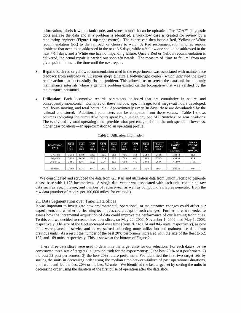
consequently monotonic. Examples of these include, age, mileage, total megawatt hours developed, total hours moving, and total hours idle. Approximately every 30 days, these are downloaded by the railroad and stored. Additional parameters can be computed from these values. Table I shows columns indicating the cumulative hours spent by a unit in any one of 8 ‘notches’ or gear positions. These, divided by total operating time, provide what percentage of time the unit spends in lower vs. higher gear positions—an approximation to an operating profile.

Table I. Utilization Information

DOWNLOAD DATE

CUM N1 HS

CUM N2

HRS

CUM N3

HRS

CUM N4

HRS

CUM N5

HRS

CUM N6

HRS

CUM N7

HRS

CUM N8

HRS

CUM BRAKE

HRS

CUM ENGINE

HRS MOVING

DELTA ENGINE

HRS MOVING

5-Apr-03 361.4 148.6 136.5 102.5 91.2 72.6 46.6 254.0 274.8 1,488.13 31.8

2-Apr-03 351.6 142.6 130.8 100.4 89.5 71.3 46.1 253.5 270.5 1,456.30 43.4

28-Mar-03 340.5 138.4 127.0 97.4 86.5 68.8 44.3 247.4 262.6 1,412.90 116.5

… …

28-Jul-01 259.0 113.1 97.7 79.5 72.1 55.9 36.4 176.0 196.4 1,086.24 0.0

We consolidated and scrubbed the data from GE Rail and utilization data from Union Pacific to generate

a case base with 1,178 locomotives. A single data vector was associated with each unit, containing raw data such as age, mileage, and number of repairs/year as well as compound variables generated from the raw data (number of repairs per 100,000 miles, for example). 2.1 Data Segmentation over Time: Data Slices It was important to investigate how environmental, operational, or maintenance changes could affect our experiments and whether our learning techniques could adapt to such changes. Furthermore, we needed to assess how the incremental acquisition of data could improve the performance of our learning techniques. To this end we decided to create three data slices, on May 22, 2002, November 1, 2002, and May 1, 2003, respectively. The size of the fleet increased over time (from 262 to 634 and 845 units, respectively), as new units were placed in service and as we started collecting more utilization and maintenance data from previous units. As a result the number of the best 20% performers increased with the size of the fleet to 52, 127, and 169 units, respectively. This is shown at the bottom of Figure 2.

These three data slices were used to determine the target units for our selection. For each data slice we constructed three sets of targets (i.e., ground truth for the experiments): 1) the best 20 % past performers; 2) the best 52 past performers; 3) the best 20% future performers. We identified the first two target sets by sorting the units in decreasing order using the median time-between-failure of past operational durations, until we identified the best 20% or the best 52 units. We identified the last target set by sorting the units in decreasing order using the duration of the first pulse of operation after the data slice.

Figure 2. Time Segmentation

2.2 Performance Metrics The primary metric was the ability of a classifier to select the best N units in any given slice (i.e., its precision). We investigated two approaches to define the top ‘N’ units.

1) Fixed Percentage Approach: In the fixed percentage approach, the task of the classifier was to pick the top 20% of units. The actual number of units to be selected increased with fleet size as we progressed from slice 1 to slice 3.

2) Fixed Number Approach: In the fixed number of units approach, the actual number of units to be selected was kept constant. In the experiments, the number used was 20% of the first slice, i.e. 52 units. As the size of the fleet increased, the selection task got harder as 52 units represented 12% and 6% of the fleet size in slices 2 and 3 respectively.

2.3 Baselines Two baselines were calculated to measure the increase in capability provided by the collective mind algorithms.

1) Random: The first baseline measured the expected performance if selection of the best N units were done randomly. This obviously represented a worst-case scenario.

2) Heuristics: The second baseline was the best performance achieved by single or multiple heuristics (based on any of the measured or calculated parameters) which we used to rank the fleet and pick the best N units.

3. Fuzzy Instance Based Models Instance-Based Models (IBM) relies on a collection of previously experienced data stored in their raw representation. Unlike Case-Based Reasoning (CBR), they do not need to be refined, abstracted and organized as cases. Like CBR, IBM is an analogical approach to reasoning since it relies upon finding previous instances of similar problems and uses them to create an ensemble of local models. Hence the definition of similarity plays a critical role in the performance of IBM’s. Typically, similarity will be a dynamic concept and will change over the use of the IBM. Therefore, it is important to apply learning methodologies to define and adapt it. Furthermore, the concept of similarity is fuzzy, rather than crisply defined, creating the need to allow for some degree of vagueness in its evaluation. We addressed this issue by evolving the design of a similarity function in conjunction with the design of the attribute space in which the similarity was evaluated. Specifically, we used the following four steps: 1) Retrieval of similar instances from the database (DB); 2) Evaluation of similarity measures between the probe and the retrieved instances; 3) Creation of local models using the most similar instances (weighted by their similarity measures); 4) Aggregation of outputs of local models to probe.

A description of the Fuzzy Instance Based Models (F-IBM) and some preliminary results were described in (Bonissone et al 2005a; 2005b). The F-IBM process is summarized in Figure 3 and detailed in the following four subsections.

Figure 3. Fuzzy Instance Based Models

3.1 Retrieval We look for all instances in the DB that have a behavior similar to the probe. These instances are the potential peers of the probe. The peers and probe can be seen as points in an n-dimensional feature space. For instance, let us assume that a probe Q is characterized by an n-dimensional vector of feature values

QX , and O(Q)=[D1,Q , D2,Q, …, Dk(Q),Q] the history of its operational availability durations:

],...,;,...,[)](;[ ),(,1,,1 QQkQQnQQ DDxxQOXQ == (1)

Each other unit ui in the fleet has a similar characterization: ],...,, ;,...,,[)](;[ ),(,2,1,,2,1 jjkjjjnjjjjj DDDxxxuOXu == (2)

For each dimension i we define a Truncated Generalized Bell Function,TGBFi(xi;ai,bi,ci), centered at the value of the probe ci,, which represents the degree of similarity along that dimension. Specifically:

>

−+

−+=

−−

otherwise

a

cxif

a

cxcbaxTGBF

ii b

i

ii

b

i

ii

iiiii

0

1 1),,;(

1212

ε (3)

where ε is the truncation parameter, e.g. ε =10-5. Since the parameters ci in each TGBFi are determined by the values of the probe, each TGBFi has only

two free parameters, ai and bi, to control its spread and curvature. In a coarse retrieval step, we extract an instance in the DB if all of its features are within the support of the TGBF’s. 3.2 Weighted Similarity Evaluation Each TGBFi is a membership function representing the partial degree of satisfaction of constraint Ai(xi). Thus, it represents the closeness of the instance around the probe value for that particular attribute. For a given peer Pj, we evaluate the function ),, ;( ,,, Qiiijiiji xbaxTGBFS = along each potential attribute i. The

values (ai, bi) are design choices manually initialized, and later refined by the EA’s. Since we want the most similar instances to be the closest to the probe along all n attributes, we use a similarity measure defined as the intersection of the constraint-satisfaction values. Furthermore, to represent the different relevance that each criterion should have in the evaluation of similarity, we attach a weight wi to each attribute Ai. Therefore, we extend the notion of a similarity measure between Pj and the probe Q as a weighted minimum operator:

( )[ ]{ } ( )[ ]{ }),,;(,1 ,1 ,,1,1 Qiiijiiiniiji

nij xbaxTGBFwMaxMinSwMaxMinS −=−= ==

(4)

where wi ∈ [0,1]. The set of values for the weights {wi} and parameters {(ai , bi )} are critical design choices that impact the proper selection of peers. In this section we assume a manual setting of these values. In the next subsection, we will explain their selection using evolutionary search. 3.3 Creation of Local Models The idea of avoiding pre-constructed models and creating a local model when needed can be traced back to memory-based approaches (Atkenson, 1992; Atkenson et al. 1997) and lazy-learning (Bersini et al, 1998). Within the scope of this paper, we will focus on the creation of local predictive models used to forecast each unit’s remaining life. First, we use each local model to generate an estimated value of the predicted variable. Then, we use an aggregation mechanism based on the similarities of the peers to determine the final output.

For instance, let us assume that for a given probe Q we have retrieved m peers, Pj(Q), j=1,…, m. Each peer Pj(Q) has a similarity measure Sj with the probe. Furthermore, each peer Pj has a track record of operational availability between failures O(Pj) = [D1,j , D2,j , …, Dk(j),j ]. Each peer Pj(Q) will have k(j) availability pulses in its track history. For each peer Pj, the goal is to determine the duration of the next availability duration Dk(j)+1,j. Then we want to combine the prediction of all the peers {Dk(j)+1,j} (j=1,…, m) to estimate the availability duration for the probe Q. Since there were not enough historical data to reliably generate local regressions, we experimented with simpler models such as averages and medians. We determined that the most reliable way of generating the next availability duration Dk(j)+1,j. from the operational availability vector O(Pj)=[D1,j , D2,j , …, Dk(j),j ] was to use an exponential average that gives more relevance to the most recent information, namely:

] [where )1( ,1,1,1)(),(),(,1)( jjjjkjjkjjkjjkj DDDDDDy =×−+×=== −+ αα jt

tjkjk

tj DDjk

,

)()(

2,1 )1()1( 1)( ××−+−=−

=∑− ααα (5)

Again, critical to the performance of this model is the choice of the value of α and its best value will be determined by evolutionary search.

3.4 Aggregation Mechanism We need to combine the individual predictions {Dk(j)+1,j} (j=1,…, m) of the peers Pj(Q) to generate the prediction of the next availability duration, DNext,Q for the probe Q. We define this aggregation as the similarity weighted average, by computing the weighted average of the peers’ individual predictions using their normalized similarity to the probe as a weight:

where ,1)(

1

1, jjkjm

j j

m

j jj

QNextQ DyS

ySDy +

=

= =×

==∑

∑ (6)

This structure is similar to the Nadaraya-Watson estimator for non-parametric regressions using locally weighted averages – where the weights are the values of a kernel function K:

)(

)(

1

1

∑∑

=

=

−

×−=

m

j j

m

j jj

QxxK

yxxKy (7)

where K(x-xj) is the kernel function evaluation at the jth point. From this structural analogy, we observe that the similarity metric Sj plays the same role in the aggregation as the Kernel function K(x - xj). Based on the relationship between similarity metrics and distances (Zadeh, 1971), we conclude that Sj is a lower bound for K(x - xj).

Given the critical role played by the weights {wi}, by the search parameters {(ai, bi)} and by exponent α, it was necessary to create a methodology that could generate the best values according to our metrics (classification precision).

4. Model Optimization and Maintenance 4.1 Implementation We decided to use an evolutionary search to develop and maintain the fuzzy instance based classifier. The system was implemented using SOFT-CBR: a Self-Optimizing Fuzzy Tool for Case-Based Reasoning (Aggour, Pavese, et al. 2003). SOFT-CBR is an extensible, component-based tool with a number of pre-existing modules to implement a CBR system in Java. SOFT-CBR significantly reduced the implementation and testing cycles for these experiments, as it provided large portions of the functionality pre-built and pre-tested. SOFT-CBR is configured using an eXtensible Mark-up Language (XML) file. Changing the parameters in the file can change the attributes used to define cases, the method by which similarities are calculated, and determine what types of outputs are valid. Optimizing the engine requires the optimization of a set (or subset) of the parameters in this configuration file.

Using a wrapper methodology detailed in (Bonissone et al, 2002), we used Evolutionary Algorithms to tune the parameters of a classifier used to underwrite insurance applications. In this application, we extend evolutionary search beyond parametric tuning to include structural search, via attribute selection and weighting (Freitas, 2002). An EA is composed of a population of individuals (“chromosomes”), each of which contains a vector of elements that represent distinct tunable parameters within the FIBM configuration. The EA’s are composed of a population of individuals (“chromosomes”), each of which contains a vector of elements that represent distinct tuneable parameters within the FIBM configuration. Examples of tuneable parameters include the range of each parameter used to retrieve neighbor instances and the relative parameter weights used for similarity calculation. The EA’s used two types of mutation operators (Gaussian and uniform), and no crossover. Its population (with 100 individuals) was evolved over 200 generations.

4.2 Chromosome Representation. Each chromosome defines an instance of the attribute space used by the associated classifier by specifying a vector of weights [ ] ... 21 nwww . If { }1,0∈w , we perform attribute selection, i.e., we select a crisp subset

from the universe of potential attibutes. If [ ]1,0∈w , we perform attribute weighting, i.e., we define a fuzzy

subset from the universe of potential attributes [ ] ( ) ( ) ( )[ ][ ]α , ..., ,, ,, ... 221121 nnn bababawww (8)

[ ]{ }

nU

selectionforw

weightingforw

i

i

=∈∈

U,features of universe ofy Cardinalit = n

attribute 1,0

and attribute 1,0 where

Average entialfor Expon Parameter

GBFfor Parameters)b,(a

features selected ofy cardinalit (fuzzy) = d

iii

==

∑

α

n

i iw

The first part of the chromosome, containing the weights vector [w1, w2, …, wn,], defines the attribute space (the FIBM structure) and the relevance of each attribute in evaluating similarity. The second part of the chromosome, containing the vector of pairs [(a1, b1), … (ai, bi), … (an, bn)] defines the parameter for retrieval and similarity evaluation. The last part of the chromosome, containing the parameter α, defines the forgetting factor for the local models. The fitness function is computed using a wrapper approach (Freitas, 2002). For each chromosome, represented by (8), we instantiate its corresponding FIBM. Following a leave-one-out approach, we use the FIBM to predict the expected life of the probe unit following the four steps described in the previous subsection. We repeat this process for all units in the fleet and sort them in decreasing order, using their predicted duration DNext,Q. We then select the top 20%. The fitness function of the chromosome is the precision of the classification, TP/(TP+FP). 5. Results For each set of experiments, we used the three time slices illustrated in Figure 2. As stated earlier, we wanted to test the adaptability of the learning techniques to environmental, operational, or maintenance changes. Furthermore, we wanted to determine if their performance would improve over time with

incremental data acquisition. For each start-up time, we used evolutionary algorithms to generate an optimized weighted subset of attributes to define the peers of each unit.

Successfully deployed intelligent systems must remain valid and accurate over time, while compensating for drifts and accounting for contextual changes that might otherwise render their knowledge-base stale or obsolete. In this study, we performed three sets of experiments with dynamic and static models. The dynamic models are fresher models, re-developed at each time slice by using the methodology described in the previous section. The static models were developed at time slice 1 and applied, unchanged, at time slices 2 and 3. This comparison shows the benefit of automated model updating.

5.1 Experiments 1) First Experiment Set (Top 20% Past Performers): We predict the best 20% of the fleet, based on their past performance. In this case a random selection would yield 20%. 2) Second Experiment Set (Top 52 units Past Performers): Since the size of the fleet at each start-up time was different, we repeated the same experiments keeping the number of units constant (52 units) over the three start-up times instead of keeping a constant top 20%. Thus the random selection baseline changed from [20%-20%-20%] to [20%-8%-6%], i.e., 52/262=20%; 52/634=8%; 52/845=6%. Also, given the superior performance of the evolved peers over the manually constructed peers, we decided to use the optimized peer design instead of the manual design in all subsequent experiments. 3) Third Experiment Set (Top 20% Future Performers): In the previous two experiments the targets for selection were the best-known units in the fleet based on past performance. Now we perform prediction and target the selection of the units with the best next-pulse duration. In this case a random selection would yield 20%.

5.2 Performance of Dynamic Models

For each time slice, we used the EA’s to generate an optimized weighted subset of attributes, search parameters and forgetting factor, to define the peers of each unit. We used the evolved peer approach to run three experiments. 5.2.1. First Experiment: Top 20% Past Performers: Time slice 1 (fleet size = 262 units; top 20% = 52 units): Evolved Peers outperformed both manually-designed peers and heuristics/fleet-based approach: 48% vs. 41% vs. 32%. Time slice 2 (fleet size = 634 units; top 20% = 127 units): Evolved Peers outperformed both manually-designed peers and heuristics/fleet-based approach: 56% vs. 55% vs. 46%. Time slice 3 (fleet size = 845 units; top 20% = 169 units): Evolved Peers outperformed both manually-designed peers and heuristics/fleet-based approach: 60% vs. 54% vs. 50%. 5.2.2. Second Experiment: Top 52 units Past Performers: Time slice 1 (fleet size = 262 units; top 52 units= 20%): Evolved Peers outperformed heuristic/fleet-based approach: 48.1% vs. 32% (vs. 20% random selection). Time slice 2 (fleet size = 634 units; top 52 units = 8%): Evolved Peers outperformed heuristic/fleet-based approach: 55.8% vs. 37% (vs. 8% random selection). Time slice 3 (fleet size = 845 units; top 52 units = 6%): Evolved Peers outperformed heuristic/fleet-based approach: 63.5% vs. 37% (vs. 6% random selection).

5.2.2. Third Experiment: Top 20% Future Performers: Time slice 1 (fleet size = 262 units; top 20% = 52 units): Evolved Peers outperformed both heuristic/fleet and unit’s own history-based approach: 43% vs. 32% vs. 27%. Time slice 2 (fleet size = 634 units; top 20% = 127 units): Evolved Peers outperformed both heuristic/fleet and unit’s own history-based approach: 42.2% vs. 42% vs. 34%. Time slice 3 (fleet size = 845 units; top 20% = 169 units): Evolved Peers outperformed both heuristic/fleet and unit’s own history-based approach: 55% vs. 36% vs. 34%. The last two experiments’ results are shown in Figure 4 and 5.

48.1%

55.8%

63.5%

32%37% 37%

20%

8% 6%5.0%

15.0%

25.0%

35.0%

45.0%

55.0%

65.0%

75.0%

1 2 3

Time Slices

Sel

ecti

on

Per

form

ance

Evolved Peers

Non Peer-HeuristicsRandom

10 x betterthan random1.7 x better

thanheuristics

(52 out of 262 units) (52 out of 634 units) (52 out of 845 units)

Fig. 4. Dynamic Models 2nd Experiments Fig. 5. Dynamic Models 3rd Experiments 52 Units Past Performers 20%; Future Performers

5.3 Performance of Static Models 5.3.1 First Experiment Set: Top 20% Past Performers: The models developed in time slice 1 exhibited poor precision when applied to the remaining two time slices: 48.1% → 48.41% → 47.92%. As a comparison, the dynamic models had: 48.1% → 55.60% → 60.40% precision.

5.3.2 First Experiment Set: Top 52 units Past Performers: Again, the time slice 1 models applied to the remaining two slices were inferior to the dynamic model: 48.1% → 50.00% → 46.15% compared with the refreshed, dynamic models: 48.1% → 55.80% → 63.50%.

5.3.3 Third Experiment Set: Top 20% Future Performers: This was the most difficult experiment and the original models showed significant deterioration over time: 42.85% → 25.86% → 24.81%. In contrast, the dynamic models exhibited more robust precision: 42.85% → 42.24% → 54.88%. This is illustrated in Figure 6.

Fig. 6 Dynamic Models versus Static Models in 3rd Experiment

6. Conclusions The peers designed by the Evolutionary Algorithms provided the best accuracy overall:

–60.3% = over 3 x random, 1.2 x heuristics on selection for top 20% (based on past performance) –63.5% = over 10 x random, 1.7 x heuristics on selection for top 52 units (based on past performance) –55.0% = over 2.5 x random, 1.5 x heuristics on selection for top 20% (based on future performance).

43% 42%

55%

32%

42%

36%

20% 20% 20%

27%

34% 34%

22%19% 20%

10.0%

15.0%

20.0%

25.0%

30.0%

35.0%

40.0%

45.0%

50.0%

55.0%

60.0%

1 2 3

Time Slices

Sel

ecti

on

Per

form

ance

Evolved PeersNon Peer - HeuristicsRandomOwn (Time Series)Own (Median)

2.5 x betterthan random1.5 x better

than heuristics

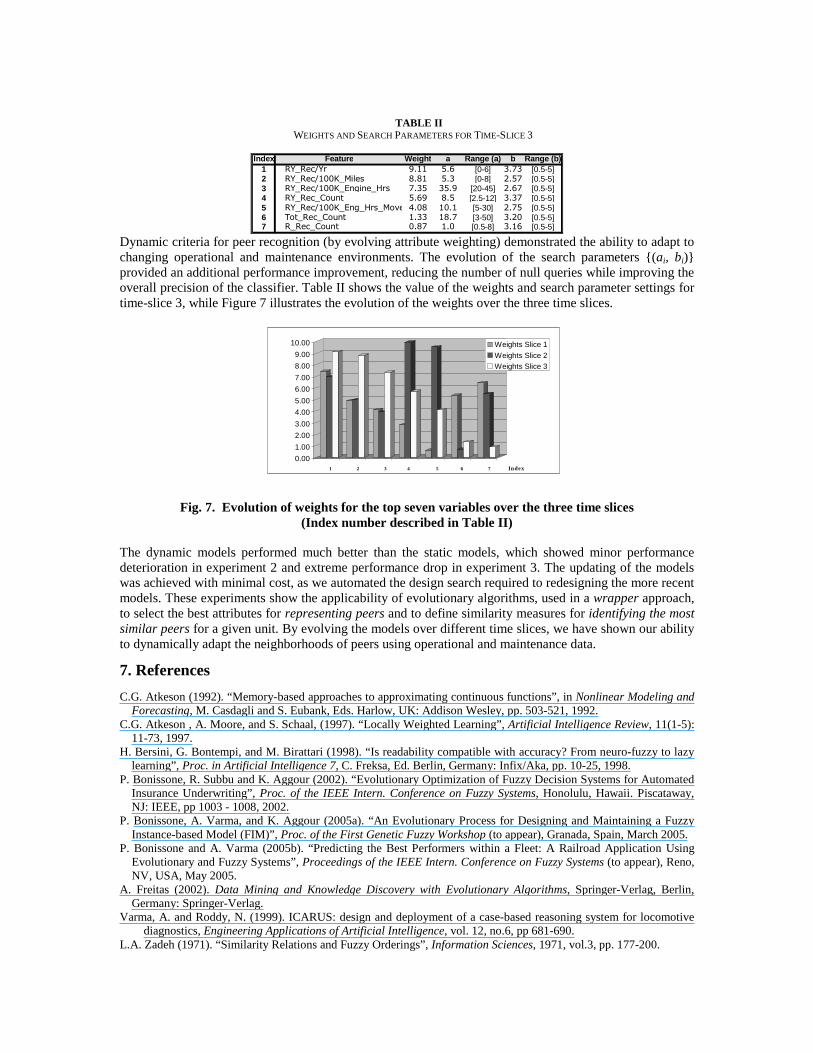
TABLE II

WEIGHTS AND SEARCH PARAMETERS FOR TIME-SLICE 3

Index Feature Weight a Range (a) b Range (b)1 RY_Rec/Yr 9.11 5.6 [0-6] 3.73 [0.5-5]2 RY_Rec/100K_Miles 8.81 5.3 [0-8] 2.57 [0.5-5]3 RY_Rec/100K_Engine_Hrs 7.35 35.9 [20-45] 2.67 [0.5-5]4 RY_Rec_Count 5.69 8.5 [2.5-12] 3.37 [0.5-5]5 RY_Rec/100K_Eng_Hrs_Move 4.08 10.1 [5-30] 2.75 [0.5-5]6 Tot_Rec_Count 1.33 18.7 [3-50] 3.20 [0.5-5]7 R_Rec_Count 0.87 1.0 [0.5-8] 3.16 [0.5-5]

Dynamic criteria for peer recognition (by evolving attribute weighting) demonstrated the ability to adapt to changing operational and maintenance environments. The evolution of the search parameters {(ai, bi)} provided an additional performance improvement, reducing the number of null queries while improving the overall precision of the classifier. Table II shows the value of the weights and search parameter settings for time-slice 3, while Figure 7 illustrates the evolution of the weights over the three time slices.

0.00

1.00

2.00

3.00

4.00

5.00

6.00

7.00

8.00

9.00

10.00

RY_REC/YR TOT_REC_COUNT

Weights Slice 1

Weights Slice 2Weights Slice 3

1 2 3 4 5 6 7 Index

Fig. 7. Evolution of weights for the top seven variables over the three time slices

(Index number described in Table II)

The dynamic models performed much better than the static models, which showed minor performance deterioration in experiment 2 and extreme performance drop in experiment 3. The updating of the models was achieved with minimal cost, as we automated the design search required to redesigning the more recent models. These experiments show the applicability of evolutionary algorithms, used in a wrapper approach, to select the best attributes for representing peers and to define similarity measures for identifying the most similar peers for a given unit. By evolving the models over different time slices, we have shown our ability to dynamically adapt the neighborhoods of peers using operational and maintenance data.

7. References C.G. Atkeson (1992). “Memory-based approaches to approximating continuous functions”, in Nonlinear Modeling and

Forecasting, M. Casdagli and S. Eubank, Eds. Harlow, UK: Addison Wesley, pp. 503-521, 1992. C.G. Atkeson , A. Moore, and S. Schaal, (1997). “Locally Weighted Learning”, Artificial Intelligence Review, 11(1-5):

11-73, 1997. H. Bersini, G. Bontempi, and M. Birattari (1998). “Is readability compatible with accuracy? From neuro-fuzzy to lazy

learning”, Proc. in Artificial Intelligence 7, C. Freksa, Ed. Berlin, Germany: Infix/Aka, pp. 10-25, 1998. P. Bonissone, R. Subbu and K. Aggour (2002). “Evolutionary Optimization of Fuzzy Decision Systems for Automated

Insurance Underwriting”, Proc. of the IEEE Intern. Conference on Fuzzy Systems, Honolulu, Hawaii. Piscataway, NJ: IEEE, pp 1003 - 1008, 2002.

P. Bonissone, A. Varma, and K. Aggour (2005a). “An Evolutionary Process for Designing and Maintaining a Fuzzy Instance-based Model (FIM)”, Proc. of the First Genetic Fuzzy Workshop (to appear), Granada, Spain, March 2005.

P. Bonissone and A. Varma (2005b). “Predicting the Best Performers within a Fleet: A Railroad Application Using Evolutionary and Fuzzy Systems”, Proceedings of the IEEE Intern. Conference on Fuzzy Systems (to appear), Reno, NV, USA, May 2005.

A. Freitas (2002). Data Mining and Knowledge Discovery with Evolutionary Algorithms, Springer-Verlag, Berlin, Germany: Springer-Verlag.

Varma, A. and Roddy, N. (1999). ICARUS: design and deployment of a case-based reasoning system for locomotive diagnostics, Engineering Applications of Artificial Intelligence, vol. 12, no.6, pp 681-690.

L.A. Zadeh (1971). “Similarity Relations and Fuzzy Orderings”, Information Sciences, 1971, vol.3, pp. 177-200.