
A fully nonlinear model for sloshing in a rotating container
30
Fluid Dynamics Research 27 (2000) 23–52 A fully nonlinear model for sloshing in a rotating container Michele La Rocca a ; * , Giampiero Sciortino a , Maria Antonietta Boniforti b a D.S.I.C., University RomaTRE, Via Corrado Segre 60, 00146, Rome, Italy b D.I.T.S., University of Rome “La Sapienza”, Via Eudossiana 18, 00184, Rome, Italy Received 23 February 1999; received in revised form 5 October 1999; accepted 13 October 1999 Abstract In this paper a theoretical and experimental analysis of sloshing in 2D and 3D free-surface congurations is performed. In particular, the case of a tank rotating around a horizontal axis has been considered. The uid is assumed to be incompressible and inviscid. A fully nonlinear mathematical model is dened by applying the variational method to the sloshing. The damping of gravity waves has been accounted by introducing a suitable dissipation function from which generalized dissipative forces are derived. A modal decomposition is then adopted for the unknowns and a dynamical system is derived to describe the evolution of the physical system. An experimental technique has been applied to select the leading modes, whose evolution characterizes the physical process, i.e. captures the most of the kinetic energy of the process. A very good agreement between experimental and numerical results conrms the validity of the methodological approach followed. c 2000 The Japan Society of Fluid Mechanics and Elsevier Science B.V. All rights reserved. PACS: 47.15.Hg; 47.35.+i; 02.60.Cb; 47.11.+j Keywords: Sloshing; Oscillating tank; Nonlinear systems; Variational methods; Dynamical systems; Karhunen–Loeve decomposition 1. Introduction Free surface sloshing in a moving container constitutes a broad class of problems of great practical importance with regard to the safety of transportations systems, such as tank trucks on highways, liquid tank cars on railroads and sloshing of liquid cargo in ocean-going vessels. Faraday (1831) well before anybody studied the sloshing instability in a vertical oscillating con- tainer. More recently, studies on sloshing were performed in order to solve stability problems caused by the movement of fuel in space vehicles. A collection of these studies and of their applications is due to Abramson (1966). The application of the classical methods of analytical mechanics to the * Corresponding author. E-mail addresses: [email protected] (M.L. Rocca), [email protected] (G. Sciortino), mab@ idra5.ing.uniroma1.it (M.A. Boniforti) 0169-5983/00/$ 20.00 c 2000 The Japan Society of Fluid Mechanics and Elsevier Science B.V. All rights reserved. PII: S0 1 6 9 - 5 9 8 3 ( 9 9 ) 0 0 0 3 9 - 8
Transcript of A fully nonlinear model for sloshing in a rotating container
Fluid Dynamics Research 27 (2000) 23–52
A fully nonlinear model for sloshing in a rotating container
Michele La Roccaa ; ∗, Giampiero Sciortinoa, Maria Antonietta BonifortibaD.S.I.C., University RomaTRE, Via Corrado Segre 60, 00146, Rome, Italy
bD.I.T.S., University of Rome “La Sapienza”, Via Eudossiana 18, 00184, Rome, Italy
Received 23 February 1999; received in revised form 5 October 1999; accepted 13 October 1999
Abstract
In this paper a theoretical and experimental analysis of sloshing in 2D and 3D free-surface con�gurations is performed.In particular, the case of a tank rotating around a horizontal axis has been considered. The uid is assumed to beincompressible and inviscid. A fully nonlinear mathematical model is de�ned by applying the variational method to thesloshing. The damping of gravity waves has been accounted by introducing a suitable dissipation function from whichgeneralized dissipative forces are derived. A modal decomposition is then adopted for the unknowns and a dynamicalsystem is derived to describe the evolution of the physical system. An experimental technique has been applied to selectthe leading modes, whose evolution characterizes the physical process, i.e. captures the most of the kinetic energy of theprocess. A very good agreement between experimental and numerical results con�rms the validity of the methodologicalapproach followed. c© 2000 The Japan Society of Fluid Mechanics and Elsevier Science B.V. All rights reserved.
PACS: 47.15.Hg; 47.35.+i; 02.60.Cb; 47.11.+j
Keywords: Sloshing; Oscillating tank; Nonlinear systems; Variational methods; Dynamical systems; Karhunen–Loevedecomposition
1. Introduction
Free surface sloshing in a moving container constitutes a broad class of problems of great practicalimportance with regard to the safety of transportations systems, such as tank trucks on highways,liquid tank cars on railroads and sloshing of liquid cargo in ocean-going vessels.Faraday (1831) well before anybody studied the sloshing instability in a vertical oscillating con-
tainer.More recently, studies on sloshing were performed in order to solve stability problems caused by
the movement of fuel in space vehicles. A collection of these studies and of their applications isdue to Abramson (1966). The application of the classical methods of analytical mechanics to the
∗ Corresponding author.E-mail addresses: [email protected] (M.L. Rocca), [email protected] (G. Sciortino), [email protected] (M.A. Boniforti)
0169-5983/00/$ 20.00 c© 2000 The Japan Society of Fluid Mechanics and Elsevier Science B.V.All rights reserved.PII: S0 1 6 9 - 5 9 8 3 ( 9 9 ) 0 0 0 3 9 - 8
24 M. La Rocca et al. / Fluid Dynamics Research 27 (2000) 23–52
sloshing was developed by Moiseiev and Rumyantsev (1968). This approach formed the basis ofsubsequent studies but has seldom been applied to practical problems due to the complexity of itsmathematical apparatus.An interesting nonlinear approach was that followed by Faltinsen (1974). He assumed the uid
inside a prismatic container to be inviscid and incompressible and solved the 2D mathematicalproblem by using a perturbation technique, applied to the potential formulation.The potential formulation is often used in studying sloshing as the works of Nakayama and
Washizu (1980), Flipse et al. (1980), Waterhouse (1994) and Ockendon et al. (1996) show and isa suitable mathematical model of the sloshing if the ratio H=B (H being the height of the liquidat rest and B the side of the container’s section, supposed squared) is such that: H=B¿0:1, namelyoutside of the shallow water region (Dean and Dalrymple, 1992).Recent works (Armenio and La Rocca, 1996; Armenio, 1997; Ushima, 1998; Kumar and Tuck-
ermann, 1994) show that viscous sloshing has been considered both from a purely numerical andanalytical–numerical point of view.The sloshing of liquids in a horizontally oscillated rectangular tank is the problem that re-
ceived the most theoretical attention (Ockendon et al., 1996) while less attention was devotedto sloshing in containers undergoing oscillating rotation. The analysis of sloshing in a rotatingcontainer is in fact more complicated than sloshing in translating containers because in the co-ordinate system attached to the tank the body forces are not conservative. This fact makes theanalytical treatment of the problem more di�cult than the case of sloshing in translatingcontainers.In the present work a theoretical and experimental analysis has been performed for sloshing in
a square-section container undergoing oscillating rotation around a horizontal axis. Starting fromthe potential formulation, a nonlinear mathematical model has been derived following a variationalapproach. Such theoretical approach has been successfully applied to water wave problems in sev-eral papers (Whitham, 1967; Miles, 1976,1988; Miles and Becker, 1988; Balk, 1996; La Rocca etal., 1997). The variational approach permits to introduce a dissipative model in a simple and e�ec-tive way (Miles, 1976). Such dissipative model makes sense for low viscous uids, while for highviscous uids a di�erent approach has to be followed (Kumar and Tuckermann, 1994; Cerda andTirapegui, 1998).Due to their originality, two aspects of this work have to be highlighted.The �rst is related to the use of a calculation technique for the search of the critical points of the
functional which does not requires any approximation linked to series expansion of the functionalitself in terms of the free surface elevation, as was customarily performed in previous works (Miles,1976,1988; Miles and Becker, 1988; La Rocca et al., 1998).The second is related to a particular experimental technique used in order to obtain information
needed to characterize a low-dimensional dynamical system through the selection of the so-calledleading modes: namely, the modes whose evolution captures most of the kinetic energy of theprocess. This experimental information was obtained by using a suitable computational techniquebased on the Karhunen–Loeve decomposition (Sirovich, 1991) of the free surface.The experimental part of this work consisted in the analysis of some sloshing con�gurations
reproduced by an experimental setup in which the frequency was varied and the amplitude ofthe oscillating rotation kept constant. The experimental analysis was used also to validate thepresent approach through the comparison of the numerical and the experimental results. A very
M. La Rocca et al. / Fluid Dynamics Research 27 (2000) 23–52 25
good agreement has been obtained, which con�rms the validity of the methodological approachfollowed.This paper is structured in the following way: in the following section (second section) the
mathematical formulation of the problem is de�ned and the modal decomposition for the free surfaceand the velocity potential are introduced. In the third section the variational approach is describedand, after introducing a suitable dissipation model, the evolution equations for the coe�cients ofthe adopted decomposition are obtained. In the fourth section the technique for the evaluation ofthe damping coe�cients is described while the truncation criterion, based on the Karhunen–Loevedecomposition is described in the �fth section. The sixth section describes the experimental setup.The seventh section describes the experimental technique of selection of the leading modes. The lasttwo sections are concerned, respectively, with the analysis of results and the concluding remarks.Appendix A gives some mathematical details not reported in the body of the paper.
2. Formulation of the problem
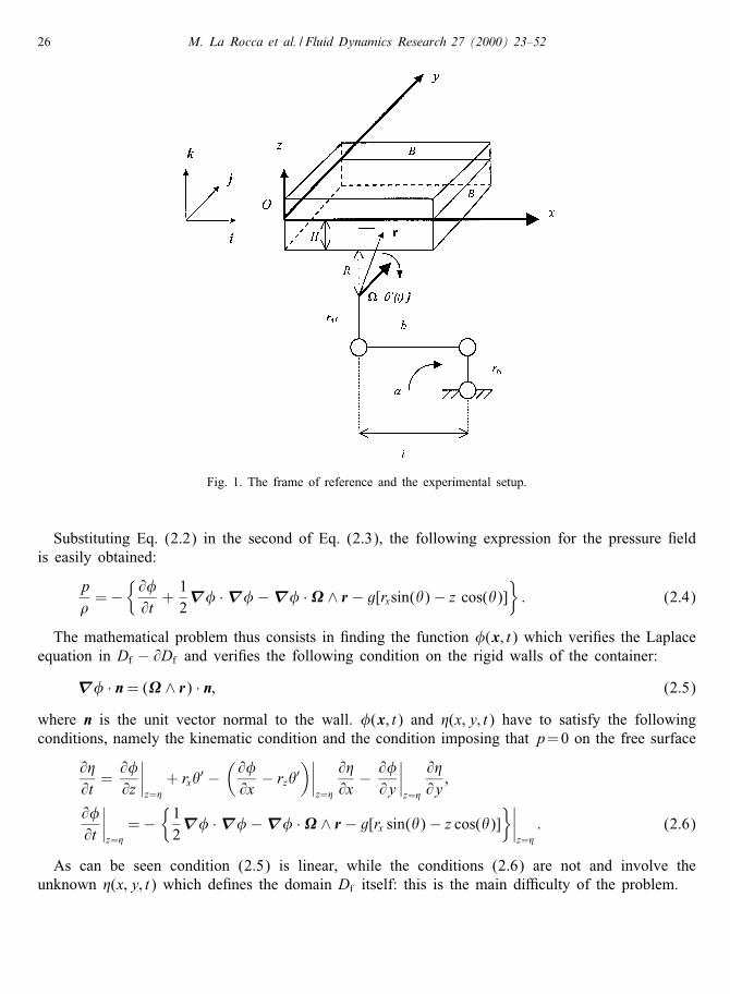
Let (C; p) be, respectively, the velocity and the pressure �eld inside a prismatic oscillating containerof square section, �lled with an incompressible uid of density � up to a level H at rest.Let the frame of reference Oxyz with the corresponding unit vectors {i; j; k} be attached to the
container, as shown in Fig. 1. In an inertial frame of reference the absolute velocity of the uidparticle is expressed by
C= Cr + ∧ r; (2.1)
where Cr is the velocity of the uid particle relative to the frame of reference Oxyz; = �′(t) j isthe assigned angular velocity of the container and
r ≡ rxi + ryj + rzk = (x − B=2)i + (y − B=2) j + (R+ H + z)kis the vector joining a �xed point of the rotation axis to the uid particle, R; B being de�ned in Fig. 1.The superscript ′ denotes ordinary di�erentiation with respect to the time t.Assuming that the velocity �eld C can be derived from a scalar potential function �=�(x; t) (x ≡
xi + yj + zk), as C=B�, it follows from Eq. (2.1) that:
Cr =B�− ∧ r: (2.2)
The Laplace equation for the potential �(x; t) and the Euler equation for the relative velocity Crand the pressure p have to be satis�ed inside the uid domain Df
B2�= 0;DCrDt
+ 2 ∧ Cr +′ ∧ r + ∧ ( ∧ r) = f − 1�Bp; (2.3)
where f = gB((x − B=2)sin(�)− z cos(�)).The uid domain Df is de�ned by
Df = {(x; y; z) | x ∈ [0; B]; y ∈ [0; B]; z ∈ [− H; �(x; y; t)];where �(x; y; t) is the unknown free surface elevation.
26 M. La Rocca et al. / Fluid Dynamics Research 27 (2000) 23–52
Fig. 1. The frame of reference and the experimental setup.
Substituting Eq. (2.2) in the second of Eq. (2.3), the following expression for the pressure �eldis easily obtained:
p�=−
{@�@t+12B� ·B�−B� · ∧ r − g[rxsin(�)− z cos(�)]
}: (2.4)
The mathematical problem thus consists in �nding the function �(x; t) which veri�es the Laplaceequation in Df − @Df and veri�es the following condition on the rigid walls of the container:
B� · n = ( ∧ r) · n; (2.5)
where n is the unit vector normal to the wall. �(x; t) and �(x; y; t) have to satisfy the followingconditions, namely the kinematic condition and the condition imposing that p=0 on the free surface
@�@t=@�@z
∣∣∣∣z=�+ rx�′ −
(@�@x
− rz�′)∣∣∣∣
z=�
@�@x
− @�@y
∣∣∣∣z=�
@�@y;
@�@t
∣∣∣∣z=�=−
{12B� ·B�−B� · ∧ r − g[rx sin(�)− z cos(�)]
}∣∣∣∣z=�: (2.6)
As can be seen condition (2.5) is linear, while the conditions (2.6) are not and involve theunknown �(x; y; t) which de�nes the domain Df itself: this is the main di�culty of the problem.
M. La Rocca et al. / Fluid Dynamics Research 27 (2000) 23–52 27
In any case it is useful to decompose the potential � into the sum of a particular solution �pof the Laplace equation which satis�es the linear boundary condition (2.5) and an unknown ’(x; t)which a priori satis�es homogeneous boundary conditions (B’ · n = 0) on the rigid walls and isharmonic in Df − @Df
�(x; t) = �p (x; t) + ’(x; t): (2.7)
The function ’(x; t) must be obviously determined by requiring the ful�llment of the nonlinearboundary conditions (2.6). The function �p (x; t) can be expressed as
�p (x; t) ≡ �′(t)�p0(x); (2.8)
where �p0 (x) is a known function whose analytical expression is given in Appendix A. The unknown’(x; t) can be expanded into the series
’(x; t) ≡∞∑n=0
∞∑m=0
Anm(t) cos(�nx) cos(�my)cosh[�nm(H + z)]cosh(�nmH)
; (2.9)
where �n ≡ n�=B; �m ≡ m�=B; �nm ≡ √�2n + �2m.
The linearization of the �rst of Eq. (2.6)
@�@t= �′(t)
(x − B
2+@�p0@z
∣∣∣∣z=0
)+@’@z
∣∣∣∣z=0
suggests the adoption of the following expansion for �:
� (x; y; t) ≡ �(t)(x − B
2+@�p0@z
∣∣∣∣z=0
)+
∞∑n=0
∞∑m=0
Qnm(t) cos(�nx) cos(�my): (2.10)
To the authors knowledge, such an expansion has never been used in other works. The di�erencewith a simple Fourier expansion consists in the number of modes necessary to obtain a satisfactoryrepresentation of the free surface. Adopting expansion (2.10) this number of modes has been foundto be much lower than that required for a simple Fourier expansion. In fact, for very low valuesof the amplitude and the frequency of the imposed oscillation, the free surface remains sensiblyhorizontal in the absolute frame of reference. As a consequence, in the adopted frame of reference,the free surface is expressed by the equation: �(x; y; t) ' �(t)(x − B=2). Then expansion (2.10)permits to eliminate the modes necessary to represent the curve �(t)(x − B=2).The amplitude coe�cients Anm(t) and Qnm(t) are unknown and must be determined through the
ful�llment of the nonlinear boundary conditions (2.6).
3. Dynamical system approach
Using N (u) = 0, where u ≡ (’; �), to denote the problem de�ned by the Laplace equation (2.3),the boundary conditions (2.5), (2.6) and assigned initial conditions, for t= t1, it is possible to de�nea suitable functional F = F(u) such that its �rst variation �F(u) ≡ (grad F(u); �u) coincides with(N (u); �u). The term (grad F(u); �u) indicates the linear application of grad F(u) on �u. In thissense, the critical points of the functional F(u) are the solutions of the problem N (u) = 0 andviceversa (Tonti, 1984). It is to be noted that F(u) is not univocally de�ned when the problem
28 M. La Rocca et al. / Fluid Dynamics Research 27 (2000) 23–52
N (u)= 0 is given. For the problem examined, a suitable choice of F(u) is the following (Whitham,1974):
F =∫ t2
t1dt∫Dfp dDf : (3.1)
where p is the pressure �eld.By using Eq. (2.4), F can be explicitly written as
F(’; �) =−�∫ t2
t1dt∫ B
0dx∫ B
0dy∫ �(x;y; t)
−Hdz
×{@�@t+12B� ·B�−B� ·− g[rx sin(�)− z cos(�)]
}: (3.2)
The function u ≡ (’; �), which makes the �rst variation �F equal to zero, gives the solution ofthe problem N (u) = 0 for t16t6t2.By using expansions (2.9), (2.10) and substituting them in Eq. (3.2), the functional F is expressed
as a function of the vectors A(t) ≡ {Anm(t)}n;m=0;1; ::: and Q(t) ≡ {Qnm(t)}n;m=0;1; ::: and the criticalpoints of the functional F can be obtained directly by using the Lagrange equations. In order toaccount for the damping of the gravity waves, generalized dissipative forces can be introducedby means of a dissipation function G = G(A′;Q′; ) (Ceschia and Nabergoj, 1978) de�ned in thefollowing. As a consequence, the Lagrange equations can be modi�ed in the following way:
ddt@L@A′ −
@L@A
=@G@A′ ;
ddt@L@Q′ −
@L@Q
=@G@Q′ ; (3.3)
where
L= L(A′;A;Q;t) ≡∫Df ;p dDf : (3.4)
The explicit calculation of L is performed by using Eq. (2.4) and de�nition (3.4) noting that Ldepends on Q by means of � (see de�nition (2.10)). The dependence of � on Q, for the sake ofsimplicity, will be denoted by �(Q; t) whenever necessary.Formally, Eqs. (3.3) constitute a system of in�nite �rst-order nonlinear di�erential equations in a
non-normal form. In order to integrate such a system, it is necessary to consider a �nite number ofequations, thus obtaining a low-dimensional dynamical system.The mathematical structure of Eqs. (3.3) is strongly simpli�ed if the generalized coordinates
Anm; Qnm are denoted by using only one index: i.e. Anm → Ai; Qnm → Qi (i = i(n; m) is a suitablefunction of the indices n; m) because it is possible to introduce a matrix formalism. After introducingthis notation, the Lagrangian L is expressed in the following way:
L=∑i
A′i 〈Mi(�(Q; t); x; y)〉+ 〈N (A;�(Q; t); x; y; t)〉; (3.5)
where the operator 〈•〉 is de�ned as: 〈•〉 ≡ ∫ B0
∫ B0 • dx dy and Mi(�(Q; t); x; y) and N (A;�(Q; t); x; y; t)
are nonlinear functions of the variables A; �(Q; t); x; y; t, explicitly de�ned in Appendix A.
M. La Rocca et al. / Fluid Dynamics Research 27 (2000) 23–52 29
Eq. (3.3) thus take on the following form:
∑j
⟨@Mi
@�@�@Qj
⟩Q′j +
⟨@Mi
@�@�@t
∣∣∣∣Q=const
⟩−⟨@N@Ai
⟩=@G@A′
i;
∑j
⟨@Mj
@�@�@Qi
⟩A′j +
⟨@N@�
@�@Qi
⟩=− @G
@Q′i; (3.6)
where i = 0; 1; : : : . Putting:
@M@Q
≡((⟨
@Mi
@�@�@Qj
⟩));
@M@Q
T
≡((⟨
@Mj
@�@�@Qi
⟩));
P ≡(⟨
@Mi
@�@�@t
∣∣∣∣Q=const
⟩);
@N@A
≡(⟨@N@Ai
⟩);
@N@Q
≡(⟨@N@�
@�@Qi
⟩): (3.7)
Eqs. (3.6) become
@M@Q
·Q′ + P − @N@A
=@G@A′ ;
@M@Q
T
· A′ +@N@Q
=− @G@Q′ : (3.8)
Eqs. (3.8) are then easily put into normal form
Q′ =(@M@Q
)−1·(@N@A
− P + @G@A′
);
A′ =−(@M@Q
T)−1
·(@N@Q
+@G@Q′
): (3.9)
The explicit calculation of L is usually performed by expanding the functions Mi and N intoMacLaurin series of � (Miles, 1976, 1988; Miles and Becker, 1988; La Rocca et al.,1998). Such aprocedure makes sense for expansions of order not greater than the third, otherwise the increasingcomputational complexity is not balanced by a corresponding increasing ability of predicting nonlin-ear features. For this reason this approach can be applied to sloshing with waves of �nite but smallamplitude.

30 M. La Rocca et al. / Fluid Dynamics Research 27 (2000) 23–52
In this work a suitable computational technique has been introduced in order to avoid the afore-mentioned series expansions. The limitations on the wave amplitude are then removed and the presentapproach can be considered fully nonlinear. In a nutshell, this computational technique consists incombining a fourth-order Runge–Kutta method with the evaluation of terms (3.7) by applying theoperator 〈•〉 at each time step.To complete the description of the mathematical model, the dissipation function G has to be
de�ned. This function can be expressed as follows:
G ≡ �B2∑i
g i!2iQ′2i ; (3.10)
where i and !i are, respectively, the logarithmic decrement and the linear natural frequency of theith corresponding mode. By ith mode we mean the function:
cos(�nx)cos(�my): (3.11)
For the inviscid approximation !i is given by the well-known dispersion relationship
!i(n;m) =(g√�2n + �2mtanh
(√�2n + �2mH
))1=2: (3.12)
In order to highlight the meaning of the function G, it is appropriate to analyze the linearizedform L∗ of the Lagrangian L (3.5); by linearized form we mean that part of L from which, byapplying Eqs. (3.3), linear di�erential equations for the unknown A and Q are derived.Omitting some heavy calculations, the following expression for L∗ is �nally obtained:
L∗ = �B2∑i
(A′iQi +
!2i2gA2i + g
Q 2i
2+Fi(t)Qi
); (3.13)
where Fi(t) is de�ned as follows:
Fi(n;m)(t) ≡ dnm
B
∫ B
0
(�′′(t)�p0(x; 0) + g�(t)
@�p0@z
∣∣∣∣z=0
)cos(�nx) dx (3.14)
and dnm is de�ned in the following way:
dnm = 1; n= m= 0;dnm = 2; n 6= 0; m= 0;dnm = 0; m 6= 0:
(3.15)
The e�ect of G on Eqs. (3.3) applied to L∗ consists only in the addition of a “viscous term”,without any modi�cation of the forcing terms. In fact, by applying Eqs. (3.3) to L∗ and eliminatingAi(t), the following di�erential equations for Qi(t) are �nally obtained:
d2Qidt2
+ 2 idQidt
+ !2i Qi =−!2i
gFi(t): (3.16)
The asymptotic analytical expression for Qi(n;m)(t) is then given by
Qi(t) =−!2i
g
∫ t
t0
e− i(t−�)√!2i − 2i
sin[√!2i − 2i (t − �)
]Fi(�) d�: (3.17)
Solutions (3.17) of Eqs. (3.16) allow a good approximation to be obtained for the free surfaceelevation only if |�(t)|�1 and far from resonance phenomena.
M. La Rocca et al. / Fluid Dynamics Research 27 (2000) 23–52 31
The calculation of the damping coe�cients i is performed starting from a suitable viscous dis-persion relationship, which is described in the next section.
4. Evaluation of the damping coe�cients
A realistic description of the free surface waves in oscillating �nite containers demands the intro-duction of a suitable model of the damping rate of surface waves.There are two main theoretical approaches to the quantitative calculation of the damping rate: the
�rst consists in de�ning a suitable linear eigenvalue problem which furnishes a dispersion relationshipbetween the wave vector � ≡ (�n; �m) of the normal mode and the complex pulsation � (Martelet al., 1998). The second consists in calculating the ratio between the dissipated and the total energyof the uid motion (Miles, 1967; Miles and Henderson, 1998; Henderson and Miles, 1994).Considering the �rst approach in order to estimate the damping rate of surface waves, the following
velocity and pressure �elds:
u ≡ U (z) sin(�nx) cos(�my)e−I�t ;v ≡ V (z) cos(�nx) sin(�my)e−I�t ;w ≡ W (z) cos(�nx) cos(�my)e−I�t ;p ≡ pd(x; y; z; t)− �gz;pd ≡ P(z) cos(�nx) cos(�my)e−I�t (4.1)
are introduced in the linearized Navier–Stokes equations and in the continuity equation (I is de�nedas I ≡ √−1). In order to obtain a viscous dispersion relationship, the following linear homogeneousboundary conditions are considered:
u|z=−H = v|z=−H = w|z=−H = 0;
pd|z=0 − �g�− 2�@w@z
∣∣∣∣z=0= 0;
(@u@z+@w@x
)∣∣∣∣z=0=(@v@z+@w@y
)∣∣∣∣z=0
= 0;
@�@t= w|z=0 : (4.2)
The �rst three conditions of Eq. (4.2) represent the no-slip condition on the bottom of the do-main considered, which is assumed to be unbounded in the x and y directions. This assumption isequivalent to neglecting the e�ects of the container lateral walls on the dissipation rate and mustbe considered a working hypothesis. On the other hand, the purpose of introducing such dissipativemodel is to simulate an important and experimentally detected feature of the sloshing: after a transientthe spectrum of the time history of the free surface does not exhibit peaks in correspondence of the
32 M. La Rocca et al. / Fluid Dynamics Research 27 (2000) 23–52
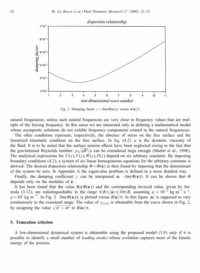
Fig. 2. Damping factor = |Im(�(�))| versus B|�|=�.
natural frequencies, unless such natural frequencies are very close to frequency values that are mul-tiple of the forcing frequency. In this sense we are interested only in de�ning a mathematical modelwhose asymptotic solutions do not exhibit frequency components related to the natural frequencies.The other conditions represent, respectively, the absence of stress on the free surface and the
linearized kinematic condition on the free surface. In Eq. (4.2) � is the dynamic viscosity ofthe uid. It is to be noted that the surface tension e�ects have been neglected owing to the fact thatthe gravitational Reynolds number: �
√gB3=� can be considered large enough (Martel et al., 1998).
The analytical expressions for U (z); V (z); W (z); P(z) depend on six arbitrary constants. By imposingboundary conditions (4.2), a system of six linear homogeneous equations for the arbitrary constants isderived. The desired dispersion relationship �=�(�) is then found by imposing that the determinantof the system be zero. In Appendix A the eigenvalue problem is de�ned in a more detailed way.Finally, the damping coe�cient i can be interpreted as −Im(�(�)). It can be shown that �
depends only on the modulus of � .It has been found that the value Re(�(�)) and the corresponding inviscid value, given by for-
mula (3.12), are indistinguishable in the range �=B6|�|610�=B, assuming � = 10−3 kg m−1 s−1,�=103 kg m−3. In Fig. 2 |Im(�(�))| is plotted versus B|�|=�. In this �gure |�| is supposed to varycontinuously in the examined range. The value of i(n;m) is obtainable from the curve shown in Fig. 2,by assigning the value
√n2 + m2 to B|�|=�.
5. Truncation criterion
A low-dimensional dynamical system is obtainable using the proposed model (3.9) only if it ispossible to identify a small number of leading modes whose evolution captures most of the kineticenergy of the process.
M. La Rocca et al. / Fluid Dynamics Research 27 (2000) 23–52 33
In this work an experimental technique was adopted in order to identify the leading modes. Inparticular, a Karhunen–Loeve decomposition (Sirovich, 1991) of the free surface was performed foreach case considered. Then each eigenfunction of the Karhunen–Loeve decomposition was expandedinto a series of modes (3.11). The analysis of the coe�cients of these expansions allows the contri-bution of the mode (3.11) to the energy of the examined signal to be evaluated and then to identifythe leading modes.The de�nition of the Karhunen–Loeve decomposition, applied to an assigned dynamical process
p(x; y; t), requires the solution of the following integral equation:
〈K(x; y; x∗; y∗)�j(x∗; y∗)〉= �j�j(x; y); (5.1)
where
K(x; y; x∗; y∗) = limT→∞
1T
∫ T
0p(x; y; t)p(x∗; y∗; t) dt (5.2)
is the correlation function, �j(x; y) is an empirical eigenfunction and �j is the correspondingeigenvalue. The eigenvalue �j can be regarded as the energy contribution of the correspondingeigenfunction �j(x; y) to the process p(x; y; t). In fact, expanding p(x; y; t) as
p(x; y; t) =∑j
pj(t)�j(x; y)
the total mean energy of the process is given by
E = limT→∞
1T
∫ T
0〈p2(x; y; t)〉 dt = lim
T→∞1T
∫ T
0
∑i; j
pi(t)pj(t)〈�i(x; y)�j(x; y)〉 dt:
Now, as a consequence of the properties (Sirovich, 1991):
limT→∞
1T
∫ T
0pi(t)pj(t) dt = �i�ij;
〈�i(x; y)�j(x; y)〉= �ij (5.3)
(�ij is the Kronecker symbol) it follows that
E = limT→∞
1T
∫ T
0
∑i; j
pi(t)pj(t)�ij dt =∑i
�i:
In this paper the dynamical process considered is de�ned by
p(x; y; t) ≡ �(x; y; t)− �(t)(x − B
2+@�p0@z
∣∣∣∣z=0
): (5.4)
De�nition (5:4) is a consequence of Eq. (2.10).Expanding each �j (x; y) into a Fourier series, it follows that:
�j(x; y) =∑n;m
anmj1Jcos(�nx)cos(�my); (5.5)
where J is a normalization coe�cient which either takes on the value B=2 if p = p(x; y; t) or thevalue
√B=2 if p= p(x; t). It is thus possible to de�ne the following ratio:
Enm =
∑j �j(a
nmj )
2∑j �j
: (5.6)
34 M. La Rocca et al. / Fluid Dynamics Research 27 (2000) 23–52
This quantity is the index which allows the leading modes to be selected on the basis of the followingmathematical property:
Enm =limT→∞ 1
T
∫ T0 [Qnm(t)]
2 dt∑p;q (limT→∞ 1
T
∫ T0 [Qpq(t)]
2 dt)(5.7)
which is derived in Appendix A. Formula (5.7) highlights the meaning of Enm as the ratio betweenthe energy contribution furnished by the (n; m) mode to the total energy of the process and the totalenergy.It should be noted that the empirical eigenfunctions �j(x; y) have not been used to represent the
free surface and the velocity potential but to obtain information about the energy contribution thateach mode (3.11) gives to the evolution of the free surface. It is not possible to use the empiricaleigenfunctions to expand the velocity potential because it is essential that ’ be a priori harmonic.
6. Experimental setup
Experimental tests were performed at the Laboratory of Hydraulics of the Department of CivilEngineering Sciences of the University RomaTRE. As shown in Fig. 1, the experimental deviceconsists of a plexiglas tank (0:5m × 0:5m × 0:25m) placed on a massive support, anchored tothe oor in order to reduce the induced vibrations. The tank can rotate around an axis parallelto the y-axis, by virtue of a crank-rod mechanism moved by an ac electric engine. It is possibleto vary both the amplitude �0 and the fundamental frequency f of the oscillating rotation, in therange: 06�060:14 rad, 06f61:5 Hz. The law of motion �(t) is given by the following implicitanalytical expression:
[rm sin(2�ft)− rM sin(�(t))− i]2 + [rm cos(2�ft) + rM cos(�(t))− b]2 = b2; (6.1)
where rm, rM , i, b are the linear dimensions, respectively, of the little and the big crank, of thedistance between their centers and of the connecting rod (Fig. 1). It is useful to consider thefollowing expansion of �(t) in term of �0 ≡ rm=rM because it highlights the Fourier components ofthe law of motion:
�(t) = �0 sin(2�ft)− 0:31�20(1 + cos(4�ft)) + � 30 (0:16 cos(2�ft)− 0:16 cos(6�ft)+0:13 sin(2�ft)− 0:004 sin(6�ft)) + O(�40 ): (6.2)
For �0�1; �(t) ' �0 sin(2�ft).The measurements performed consist in recording the time history of the free surface elevation
at suitably chosen stations. Two distance laser recorders, attached to the tank were used to performsimultaneous measurements of the free surface elevation in order to evaluate the correlation function(5.2).All the experimental tests were performed with a �xed value of the amplitude of the oscillations �0,
i.e. �0 =0:087 rad. This value was moderate but not large, in order to prevent the liquid over owingfrom the tank.The tank, at rest in the horizontal position, was �lled with water up to a level H =0:136 m. This
value for H was chosen in order to obtain the ratio H=B (H=B = 0:272) in the range: 1106H=B61,
M. La Rocca et al. / Fluid Dynamics Research 27 (2000) 23–52 35
known as the intermediate depth region for water waves. The value H = 0:136 m leaves su�cientfree margin from the top of the tank in order to contain the water waves produced by the motionof the tank itself.Di�erent values for the fundamental frequency of the oscillations f were considered: 0:3− 0:4−
0:6 − 0:7 Hz. It is to be noted that, as the value f = 0:7 Hz is not very far from the �rst linearnatural frequency f10=!10=2�=1:04 Hz, frequencies greater than 0:7 Hz could not be experimentallyimposed on the tank owing to the large amplitude of the resulting liquid motion.
7. Selection of the leading modes
In order to integrate the dynamical system (3.9) it is necessary to de�ne a set of leading modes.In the following an experimental technique of selection of the leading modes is presented, which
is based on the Karhunen–Loeve decomposition of the free surface. The quantity that allows theleading modes to be selected is Enm (5.6). The calculation of this quantity requires a very largenumber of measurements, as will be explained in the following.A preliminary step in solving the eigenvalue problem (5.1) consists in de�ning the function K
(5.2). From an experimental point of view K can be de�ned as a four-index quantity: i.e K iscalculated at the discrete points x= i�, y= j�, x∗= r�, y∗= s� by applying de�nition (5.2) with Tlarge enough. With the present measurement setup it has been assumed that �=0:025 m. This leastdistance between the measurement points is determined by the dimensions of the laser recordersand allows the existence of leading modes with wave number �n; �m62�=(2�), i.e. n; m620 to bedetected.In order to calculate K at the discrete points x= i�, y= j�, x∗= r�, y∗= s�; (i; j; r; s=0; 1; 2; : : : ;
Np − 1); N 2p (N
2p − 1)=2 measurements would be necessary. For Np = B=� = 20 the total number of
measurements is 79 800, which is very high and time consuming if only two laser recorders areused.In this work, in order to avoid such an high number of measurements without foregoing the
experimental truncation criterion, the following experimental procedure is proposed. Two series ofmeasurements were performed along x at y = 0 and along y at x = 0, each requiring Np(Np − 1)=2measurements (i.e. 190, if Np = 20). Two correlation functions:
Kx = Kx(x; x∗); Ky = Ky(y; y∗); (7.1)
were de�ned in a discrete form, i.e. the elements Kxij; Kyij were calculated at the discrete points:x = i�, x∗ = j�, y = i�, y∗ = j�, (i; j = 0; 1; 2; : : : ; Np − 1). These correlation functions are linked,respectively, to the dynamical processes p(x; 0; t), p(0; y; t), de�ned by Eq. (5.4). Applying theKarhunen–Loeve decomposition to such processes and performing the expansion (5.5), the followingindices are obtained:
Exn =
∑j �xj(a
nxj)
2∑j �xj
; (7.2)
Eym =
∑j �yj(a
myj)
2∑j �yj
:
36 M. La Rocca et al. / Fluid Dynamics Research 27 (2000) 23–52
Coe�cient Exn can be considered as the ratio between the energy furnished by the modes with agiven n and the total energy of the process p(x; 0; t) and coe�cient Eym can be considered as theratio between the energy furnished by the modes with a given m and the total energy of the processp(0; y; t), if a suitable hypothesis is veri�ed. In order to formulate such a hypothesis, it is useful toremember property (5.7), from which the following expressions can be easily derived:
Exn =limT→∞ 1
T
∫ T0
[∑m Qnm(t)
]2 dt∑n(limT→∞ 1
T
∫ T0
[∑m Qnm(t)
]2 dt) ; (7.3)
Eym =limT→∞ 1
T
∫ T0
[∑n Qnm(t)
]2 dt∑m(limT→∞ 1
T
∫ T0
[∑n Qnm(t)
]2 dt) :Now, the above hypothesis can be formulated in the following way:
limT→∞
1T
∫ T
0
[∑m
Qnm(t)
]2dt = lim
T→∞1T
∫ T
0
∑m
[Qnm(t)]2 dt; (7.4)
limT→∞
1T
∫ T
0
[∑n
Qnm(t)
]2dt = lim
T→∞1T
∫ T
0
∑n
[Qnm(t)]2 dt:
It is evident that, if hypothesis (7.4) is veri�ed, the physical meaning of Exn and Eym is simplyexpressed by the following relationships:
Exn =∑m
Enm; (7.5)
Eym =∑n
Enm:
Unfortunately, as there are no means for verifying hypothesis (7.4) a priori, the indices Exn andEym, calculated experimentally by using formula (7.2), are used with the aforementioned physicalmeaning to select the leading modes. In order to select the leading modes, it is assumed that theindices Exn and Eym are linked to a typology of (n; m) modes in the following way: from the seriesof Exn and the series of E
ym, two sets of integers (n1; n2; : : : ; nN ), (m1; m2; : : : ; mM ), such that:∑
n=n1 ; n2 ;:::; nN
Exn / 1;
∑m=m1 ;m2 ;:::;mM
Eym / 1
are identi�ed, consequently the leading modes selected are de�ned by all the (n; m) modes, with(n; m) ∈ (n1; n2; : : : ; nN )× (m1; m2; : : : ; mM ).Hypothesis (7.4) can thus be veri�ed a posteriori, calculating directly both left- and right-hand
sides of formulas (7.4), after having integrated the dynamical system, as de�ned through the leadingmodes chosen by using the coe�cients Exn and Eym.
M. La Rocca et al. / Fluid Dynamics Research 27 (2000) 23–52 37
8. Results and discussion
8.1. Preliminary considerations
In this section a comparison between numerical and experimental results is analyzed in order tovalidate the theoretical approach followed in simulating the sloshing.First, the validity of the analytical solutions (3.17) is tested through comparison with experimental
simulations performed with f=0:3 and 0.4 Hz. Analytical solutions (3.17) are a direct consequenceof the approach followed and should be a good approximation of sloshing at low frequencies.On increasing the fundamental frequency f interesting nonlinear e�ects appear and analytical
solutions (3.17) lose their validity. The fully nonlinear mathematical model (3.9) has thus to besolved after having de�ned the leading modes by applying the technique previously described.In particular for the value f=0:6 Hz interesting nonlinear e�ects are highlighted from the analysis
of the power spectrum of the time history of the free surface at given measurement stations. However,for this value of the frequency the free surface maintains a sensibly 2D con�guration (namely the freesurface does not depend on y) despite the small disturbances imposed at the beginning of motion.The last case (f = 0:7 Hz) shows an unstable 2D con�guration of the free surface, obtainable
by avoiding any disturbance at the beginning of motion. On the other hand, small disturbances,present at the beginning of motion, cause a full 3D con�guration for the free surface (namely thefree surface depends both on x and on y).
8.2. Linear cases f = 0:3 Hz, 0.4 Hz (2D)
The values f = 0:3 Hz and 0.4 Hz have been considered in order to test the validity of linearsolutions (3.17). These values of the exciting frequency can be considered su�ciently far from the�rst natural frequency (f10 = !10=2� = 1:04 Hz) so that, although the amplitude of the oscillation(�0 = 0:087 rad) cannot strictly be considered a small parameter, it makes sense to neglect thenonlinear interactions.Analytical solutions (3.17) were obtained by solving the Lagrange equations obtained from the
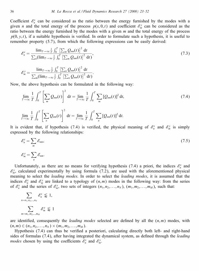
linearized Lagrangian L∗ (3.13): such solutions have to be considered a consequence of the ap-proach followed. The comparisons of the analytical solution with experimental data thus representan interesting test both for the analytical solution and for the followed approach.In Fig. 3a comparison between the numerical and experimental power spectrum of the time history
of the free surface elevation for f=0:3 Hz, in P1: x=0:15 m; y=0:25 m is shown. The agreementbetween the two spectra is very good: in particular the quantitative coincidence of the peaks is tobe noted.The existence of two secondary peaks at the frequencies 2f and 3f is clearly revealed by the ex-
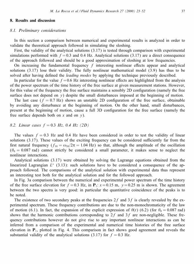
perimental spectrum. These frequency contributions are due to the non-monochromaticity of the lawof motion (6.1). In fact, the expansion of the explicit expression of �(t) (6.2) (for �0 = 0:087 rad)shows that the harmonic contributions corresponding to 2f and 3f are non-negligible. These fre-quency contributions however do not give rise to any important nonlinear interactions as can beinferred from a comparison of the experimental and numerical time histories of the free surfaceelevation in P1, plotted in Fig. 4. This comparison in fact shows good agreement and reveals thesubstantial validity of the analytical solutions (3.17) for f = 0:3 Hz.
38 M. La Rocca et al. / Fluid Dynamics Research 27 (2000) 23–52
Fig. 3. Numerical and experimental power spectrum of the time history of the free surface elevation for f = 0:3 Hz inx = 0:15 m; y = 0:25 m.
Fig. 4. Numerical and experimental time history of the free surface elevation for f = 0:3 Hz in x = 0:15 m; y = 0:25m.
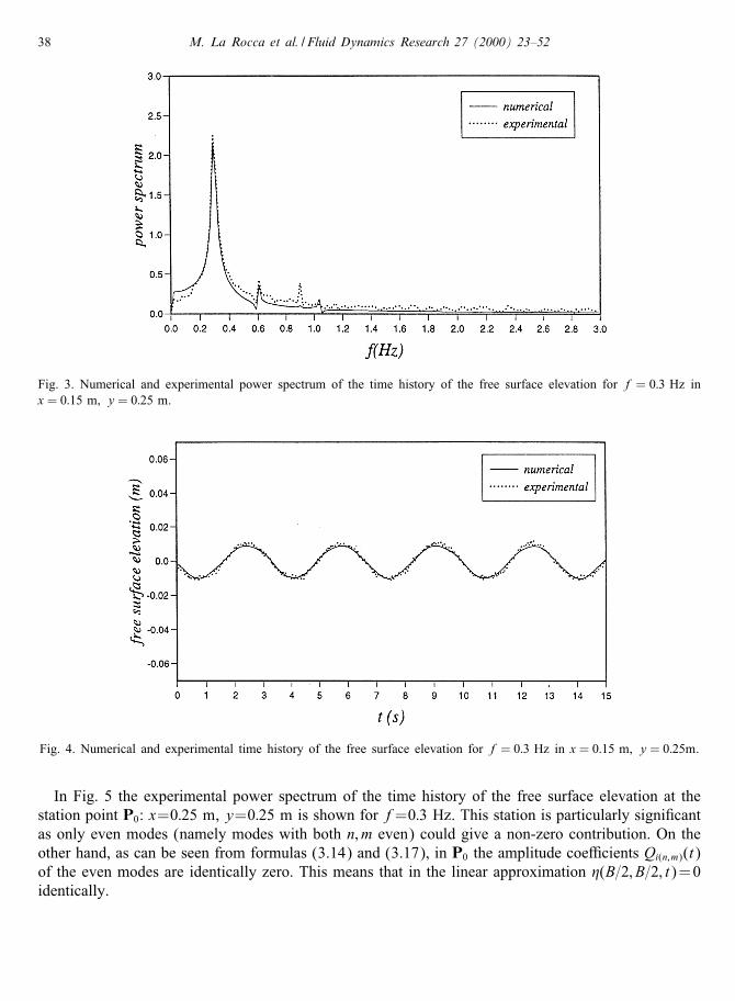
In Fig. 5 the experimental power spectrum of the time history of the free surface elevation at thestation point P0: x=0:25 m, y=0:25 m is shown for f=0:3 Hz. This station is particularly signi�cantas only even modes (namely modes with both n; m even) could give a non-zero contribution. On theother hand, as can be seen from formulas (3.14) and (3.17), in P0 the amplitude coe�cients Qi(n;m)(t)of the even modes are identically zero. This means that in the linear approximation �(B=2; B=2; t)=0identically.
M. La Rocca et al. / Fluid Dynamics Research 27 (2000) 23–52 39
Fig. 5. Experimental power spectrum of the time history of the free surface elevation for f=0:3 Hz in x=0:25 m; y=0:25 m.
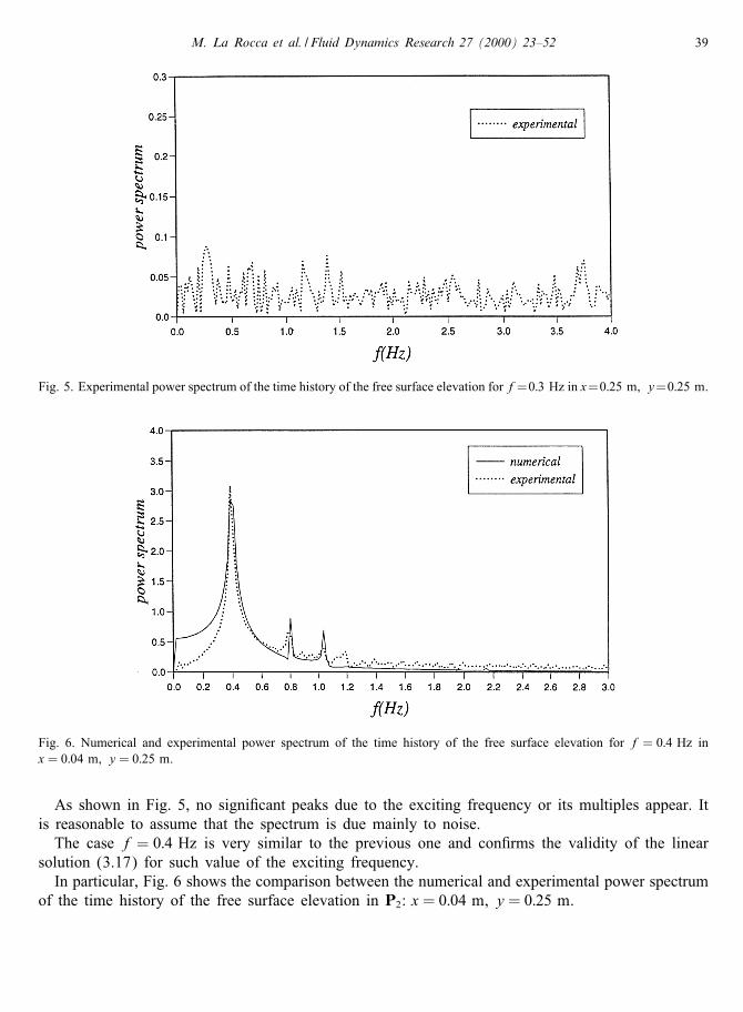
Fig. 6. Numerical and experimental power spectrum of the time history of the free surface elevation for f = 0:4 Hz inx = 0:04 m; y = 0:25 m.
As shown in Fig. 5, no signi�cant peaks due to the exciting frequency or its multiples appear. Itis reasonable to assume that the spectrum is due mainly to noise.The case f = 0:4 Hz is very similar to the previous one and con�rms the validity of the linear
solution (3.17) for such value of the exciting frequency.In particular, Fig. 6 shows the comparison between the numerical and experimental power spectrum
of the time history of the free surface elevation in P2: x = 0:04 m, y = 0:25 m.
40 M. La Rocca et al. / Fluid Dynamics Research 27 (2000) 23–52
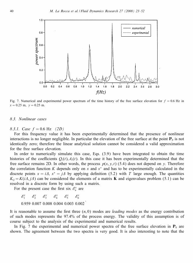
Fig. 7. Numerical and experimental power spectrum of the time history of the free surface elevation for f = 0:6 Hz inx = 0:25 m; y = 0:25 m.
8.3. Nonlinear cases
8.3.1. Case f = 0:6 Hz (2D)For this frequency value it has been experimentally determined that the presence of nonlinear
interactions is no longer negligible. In particular the elevation of the free surface at the point P0 is notidentically zero; therefore the linear analytical solution cannot be considered a valid approximationfor the free surface elevation.In order to numerically simulate this case, Eqs. (3.9) have been integrated to obtain the time
histories of the coe�cients Qi(t); Ai(t). In this case it has been experimentally determined that thefree surface remains 2D. In other words, the process p(x; y; t) (5.4) does not depend on y. Thereforethe correlation function K depends only on x and x∗ and has to be experimentally calculated in thediscrete points x = i�; x∗ = j� by applying de�nition (5.2) with T large enough. The quantitiesKij=K(i�; j�) can be considered the elements of a matrix K and eigenvalues problem (5.1) can beresolved in a discrete form by using such a matrix.For the present case the �rst six Exn are
Ex1 Ex2 Ex3 Ex4 Ex5 Ex6
0:959 0:007 0:008 0:004 0:003 0:002:
It is reasonable to assume the �rst three (n; 0) modes are leading modes as the energy contributionof such modes represents the 97:4% of the process energy. The validity of this assumption is ofcourse subject to the analysis of the experimental and numerical results.In Fig. 7 the experimental and numerical power spectra of the free surface elevation in P0 are
shown. The agreement between the two spectra is very good. It is also interesting to note that the
M. La Rocca et al. / Fluid Dynamics Research 27 (2000) 23–52 41
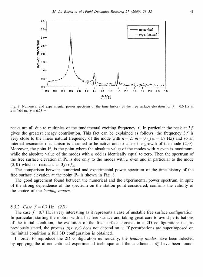
Fig. 8. Numerical and experimental power spectrum of the time history of the free surface elevation for f = 0:6 Hz inx = 0:04 m; y = 0:25 m.
peaks are all due to multiples of the fundamental exciting frequency f. In particular the peak at 3fgives the greatest energy contribution. This fact can be explained as follows: the frequency 3f isvery close to the linear natural frequency of the mode with n= 2; m= 0 (f20 = 1:7 Hz) and so aninternal resonance mechanism is assumed to be active and to cause the growth of the mode (2; 0).Moreover, the point P0 is the point where the absolute value of the modes with n even is maximum,while the absolute value of the modes with n odd is identically equal to zero. Then the spectrum ofthe free surface elevation in P0 is due only to the modes with n even and in particular to the mode(2; 0) which is resonant as 3f≈f20.The comparison between numerical and experimental power spectrum of the time history of the
free surface elevation at the point P2 is shown in Fig. 8.The good agreement found between the numerical and the experimental power spectrum, in spite
of the strong dependence of the spectrum on the station point considered, con�rms the validity ofthe choice of the leading modes.
8.3.2. Case f = 0:7 Hz (2D)The case f=0:7 Hz is very interesting as it represents a case of unstable free surface con�guration.
In particular, starting the motion with a at free surface and taking great care to avoid perturbationsof the initial condition, the evolution of the free surface consists in a 2D con�guration: i.e., aspreviously stated, the process p(x; y; t) does not depend on y. If perturbations are superimposed onthe initial condition a full 3D con�guration is obtained.In order to reproduce the 2D con�guration numerically, the leading modes have been selected
by applying the aforementioned experimental technique and the coe�cients Exn have been found.
42 M. La Rocca et al. / Fluid Dynamics Research 27 (2000) 23–52
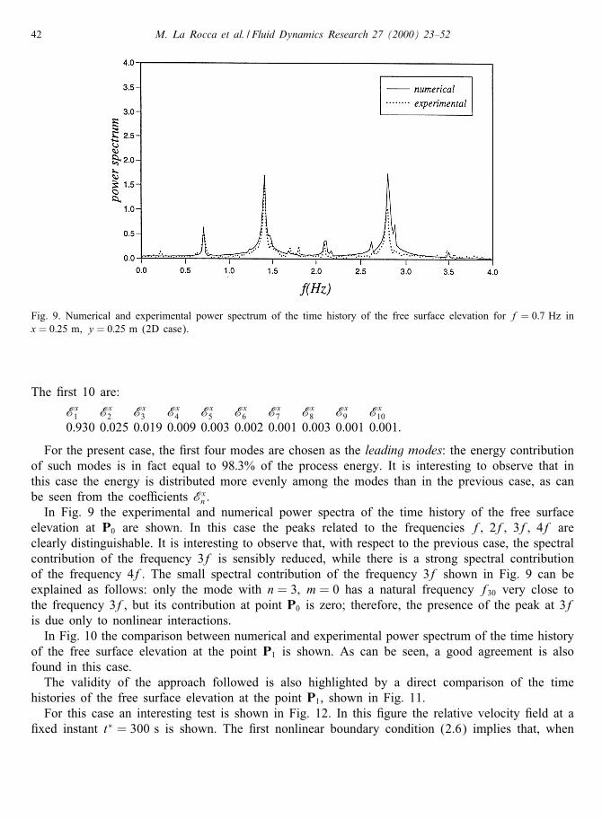
Fig. 9. Numerical and experimental power spectrum of the time history of the free surface elevation for f = 0:7 Hz inx = 0:25 m; y = 0:25 m (2D case).
The �rst 10 are:
Ex1 Ex2 Ex3 Ex4 Ex5 Ex6 Ex7 Ex8 Ex9 Ex100:930 0:025 0:019 0:009 0:003 0:002 0:001 0:003 0:001 0:001:
For the present case, the �rst four modes are chosen as the leading modes: the energy contributionof such modes is in fact equal to 98:3% of the process energy. It is interesting to observe that inthis case the energy is distributed more evenly among the modes than in the previous case, as canbe seen from the coe�cients Exn .In Fig. 9 the experimental and numerical power spectra of the time history of the free surface
elevation at P0 are shown. In this case the peaks related to the frequencies f; 2f; 3f; 4f areclearly distinguishable. It is interesting to observe that, with respect to the previous case, the spectralcontribution of the frequency 3f is sensibly reduced, while there is a strong spectral contributionof the frequency 4f. The small spectral contribution of the frequency 3f shown in Fig. 9 can beexplained as follows: only the mode with n = 3; m = 0 has a natural frequency f30 very close tothe frequency 3f, but its contribution at point P0 is zero; therefore, the presence of the peak at 3fis due only to nonlinear interactions.In Fig. 10 the comparison between numerical and experimental power spectrum of the time history
of the free surface elevation at the point P1 is shown. As can be seen, a good agreement is alsofound in this case.The validity of the approach followed is also highlighted by a direct comparison of the time
histories of the free surface elevation at the point P1, shown in Fig. 11.For this case an interesting test is shown in Fig. 12. In this �gure the relative velocity �eld at a
�xed instant t∗ = 300 s is shown. The �rst nonlinear boundary condition (2.6) implies that, when
M. La Rocca et al. / Fluid Dynamics Research 27 (2000) 23–52 43
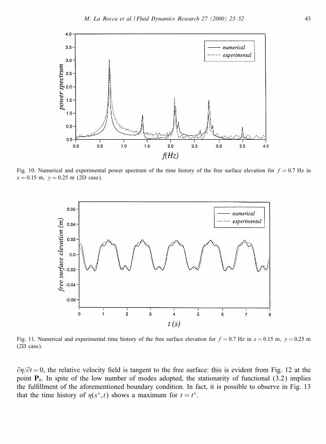
Fig. 10. Numerical and experimental power spectrum of the time history of the free surface elevation for f = 0:7 Hz inx = 0:15 m; y = 0:25 m (2D case).
Fig. 11. Numerical and experimental time history of the free surface elevation for f= 0:7 Hz in x= 0:15 m; y= 0:25 m(2D case).
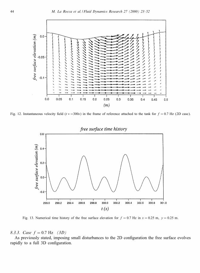
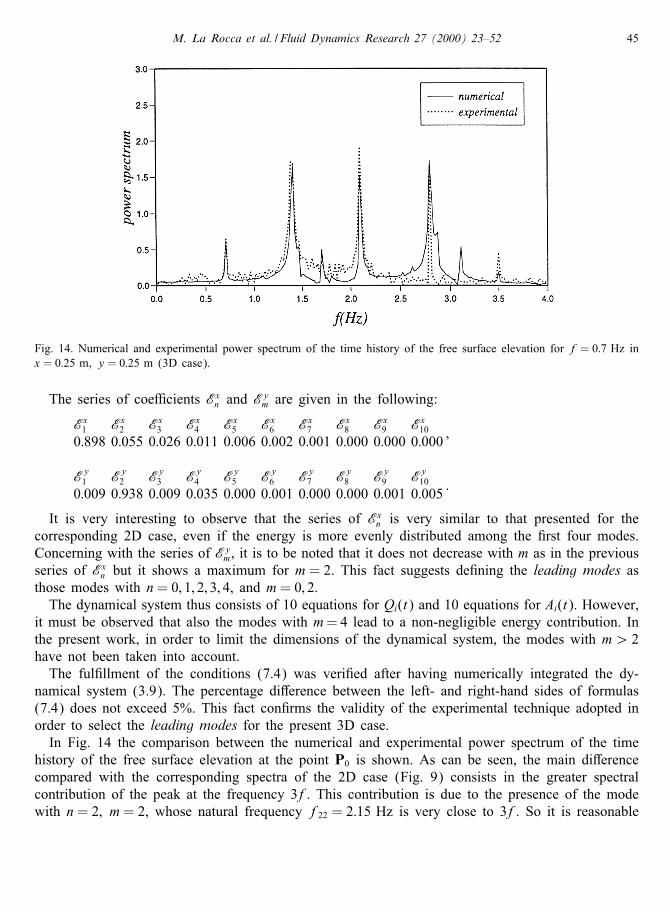
@�=@t=0, the relative velocity �eld is tangent to the free surface: this is evident from Fig. 12 at thepoint P0. In spite of the low number of modes adopted, the stationarity of functional (3.2) impliesthe ful�llment of the aforementioned boundary condition. In fact, it is possible to observe in Fig. 13that the time history of �(x∗; t) shows a maximum for t = t∗.
44 M. La Rocca et al. / Fluid Dynamics Research 27 (2000) 23–52
Fig. 12. Instantaneous velocity �eld (t ∗=300s) in the frame of reference attached to the tank for f= 0:7 Hz (2D case).
Fig. 13. Numerical time history of the free surface elevation for f = 0:7 Hz in x = 0:25 m; y = 0:25 m.
8.3.3. Case f = 0:7 Hz (3D)As previously stated, imposing small disturbances to the 2D con�guration the free surface evolves
rapidly to a full 3D con�guration.
M. La Rocca et al. / Fluid Dynamics Research 27 (2000) 23–52 45
Fig. 14. Numerical and experimental power spectrum of the time history of the free surface elevation for f = 0:7 Hz inx = 0:25 m; y = 0:25 m (3D case).
The series of coe�cients Exn and Eym are given in the following:
Ex1 Ex2 Ex3 Ex4 Ex5 Ex6 Ex7 Ex8 Ex9 Ex100:898 0:055 0:026 0:011 0:006 0:002 0:001 0:000 0:000 0:000 ;
Ey1 Ey2 Ey3 Ey4 Ey5 Ey6 Ey7 Ey8 Ey9 Ey100:009 0:938 0:009 0:035 0:000 0:001 0:000 0:000 0:001 0:005 :
It is very interesting to observe that the series of Exn is very similar to that presented for thecorresponding 2D case, even if the energy is more evenly distributed among the �rst four modes.Concerning with the series of Eym, it is to be noted that it does not decrease with m as in the previousseries of Exn but it shows a maximum for m = 2. This fact suggests de�ning the leading modes asthose modes with n= 0; 1; 2; 3; 4, and m= 0; 2.The dynamical system thus consists of 10 equations for Qi(t) and 10 equations for Ai(t). However,
it must be observed that also the modes with m=4 lead to a non-negligible energy contribution. Inthe present work, in order to limit the dimensions of the dynamical system, the modes with m¿ 2have not been taken into account.The ful�llment of the conditions (7.4) was veri�ed after having numerically integrated the dy-
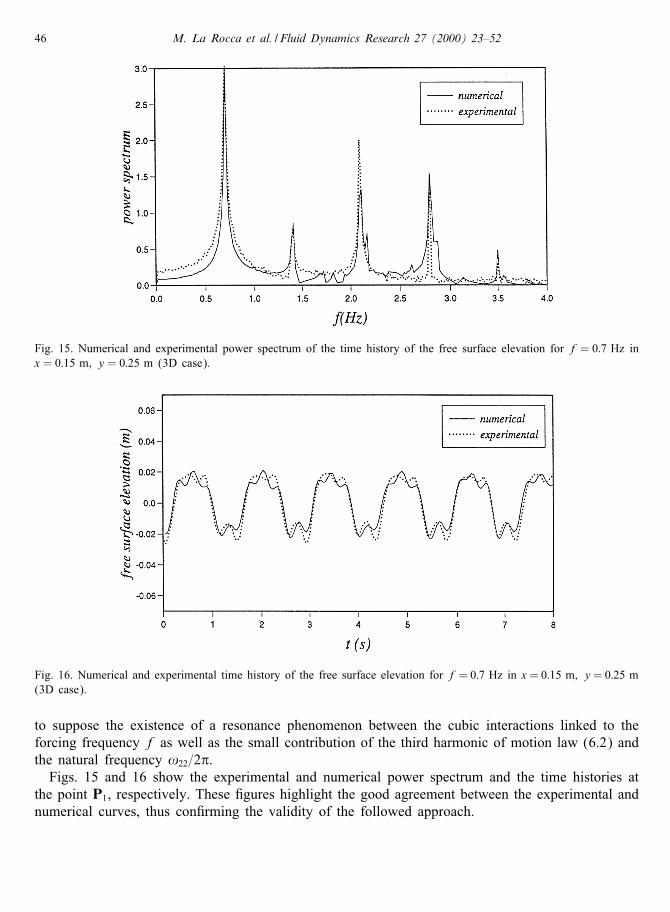
namical system (3.9). The percentage di�erence between the left- and right-hand sides of formulas(7.4) does not exceed 5%. This fact con�rms the validity of the experimental technique adopted inorder to select the leading modes for the present 3D case.In Fig. 14 the comparison between the numerical and experimental power spectrum of the time
history of the free surface elevation at the point P0 is shown. As can be seen, the main di�erencecompared with the corresponding spectra of the 2D case (Fig. 9) consists in the greater spectralcontribution of the peak at the frequency 3f. This contribution is due to the presence of the modewith n = 2; m = 2, whose natural frequency f22 = 2:15 Hz is very close to 3f. So it is reasonable
46 M. La Rocca et al. / Fluid Dynamics Research 27 (2000) 23–52
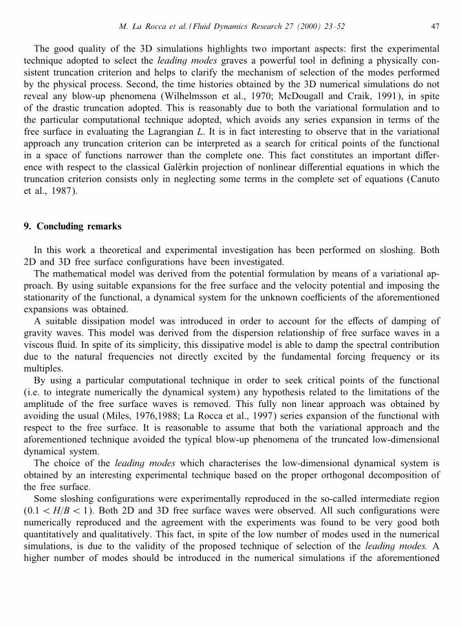
Fig. 15. Numerical and experimental power spectrum of the time history of the free surface elevation for f = 0:7 Hz inx = 0:15 m; y = 0:25 m (3D case).
Fig. 16. Numerical and experimental time history of the free surface elevation for f= 0:7 Hz in x= 0:15 m; y= 0:25 m(3D case).
to suppose the existence of a resonance phenomenon between the cubic interactions linked to theforcing frequency f as well as the small contribution of the third harmonic of motion law (6.2) andthe natural frequency !22=2�.Figs. 15 and 16 show the experimental and numerical power spectrum and the time histories at
the point P1, respectively. These �gures highlight the good agreement between the experimental andnumerical curves, thus con�rming the validity of the followed approach.
M. La Rocca et al. / Fluid Dynamics Research 27 (2000) 23–52 47
The good quality of the 3D simulations highlights two important aspects: �rst the experimentaltechnique adopted to select the leading modes graves a powerful tool in de�ning a physically con-sistent truncation criterion and helps to clarify the mechanism of selection of the modes performedby the physical process. Second, the time histories obtained by the 3D numerical simulations do notreveal any blow-up phenomena (Wilhelmsson et al., 1970; McDougall and Craik, 1991), in spiteof the drastic truncation adopted. This is reasonably due to both the variational formulation and tothe particular computational technique adopted, which avoids any series expansion in terms of thefree surface in evaluating the Lagrangian L. It is in fact interesting to observe that in the variationalapproach any truncation criterion can be interpreted as a search for critical points of the functionalin a space of functions narrower than the complete one. This fact constitutes an important di�er-ence with respect to the classical Gal�erkin projection of nonlinear di�erential equations in which thetruncation criterion consists only in neglecting some terms in the complete set of equations (Canutoet al., 1987).
9. Concluding remarks
In this work a theoretical and experimental investigation has been performed on sloshing. Both2D and 3D free surface con�gurations have been investigated.The mathematical model was derived from the potential formulation by means of a variational ap-
proach. By using suitable expansions for the free surface and the velocity potential and imposing thestationarity of the functional, a dynamical system for the unknown coe�cients of the aforementionedexpansions was obtained.A suitable dissipation model was introduced in order to account for the e�ects of damping of
gravity waves. This model was derived from the dispersion relationship of free surface waves in aviscous uid. In spite of its simplicity, this dissipative model is able to damp the spectral contributiondue to the natural frequencies not directly excited by the fundamental forcing frequency or itsmultiples.By using a particular computational technique in order to seek critical points of the functional
(i.e. to integrate numerically the dynamical system) any hypothesis related to the limitations of theamplitude of the free surface waves is removed. This fully non linear approach was obtained byavoiding the usual (Miles, 1976,1988; La Rocca et al., 1997) series expansion of the functional withrespect to the free surface. It is reasonable to assume that both the variational approach and theaforementioned technique avoided the typical blow-up phenomena of the truncated low-dimensionaldynamical system.The choice of the leading modes which characterises the low-dimensional dynamical system is
obtained by an interesting experimental technique based on the proper orthogonal decomposition ofthe free surface.Some sloshing con�gurations were experimentally reproduced in the so-called intermediate region
(0:1¡H=B¡ 1). Both 2D and 3D free surface waves were observed. All such con�gurations werenumerically reproduced and the agreement with the experiments was found to be very good bothquantitatively and qualitatively. This fact, in spite of the low number of modes used in the numericalsimulations, is due to the validity of the proposed technique of selection of the leading modes. Ahigher number of modes should be introduced in the numerical simulations if the aforementioned
48 M. La Rocca et al. / Fluid Dynamics Research 27 (2000) 23–52
technique is not applied. For the 3D simulations the number of equations constituting the dynamicalsystem (3.9) would be much greater than that obtained by applying the aforementioned technique.All these considerations con�rm the validity of the methodological approach followed in modelling
the sloshing.
Appendix A
A.1. De�nition of �p0(x)
�p0(x)≡ (R+ H)(x − B
2
)+
∞∑k=0
ak{cosh(�kx)− cosh[�k (x − B)]}sin(�kz)
−∞∑k=0
bksin[�k
(x − B
2
)]sinh(�kz); (A.1)
where
�k = �1 + 2k2H
;
�k = �1 + 2kB
;
ak =2(−1)k
�3kH sinh(�kB);
bk =4(−1)k
�3kB cosh(�kH): (A.2)
It is easy to verify that the function (A.1) is harmonic and satis�es the following properties:@�p0@x
∣∣∣∣x=0; B
= R+ H + z;
@�p0@z
∣∣∣∣z=−H
=−(x − B
2
)(A.3)
which ensure the ful�llment of the linear boundary conditions (2.5).
A.2. De�nition of Mi and N
Mi(n;m) ≡ sinh[�nm(H + �)]�nmcosh[�nmH ]
cos(�nx)cos(�my);
N ≡ �′′C(x; �) + � ′2[(x − B
2
)�p0(x; �)− G(x; �)
M. La Rocca et al. / Fluid Dynamics Research 27 (2000) 23–52 49
+12(C2x(x; �) + C2z(x; �))
]+ g
cos(�)2
�2 − g sin(�)(x − B
2
)�
+�′∑n;m
Anm(t){(x − B
2
)cos(�nx)cos(�my)
×cosh[�nm(H + �)]− 1cosh[�nmH ]
+ �nPnm(�)sin(�nx)cos(�my)
−�nRnm(x; �)sin(�nx)cos(�my) +Snm(x; �)cos(�nx)cos(�my)}
+12
∑n;m;l;p
Anm(t)Alp(t){Lnmlp(�)
×[�n�lsin(�nx)cos(�my)sin(�lx)cos(�py)+�m�pcos(�nx)sin(�my)cos(�lx)sin(�py)]
+Mnmlp(�)cos(�nx)cos(�my)cos(�lx)cos(�py)}; (A.4)
where
C(x; �) =∫ �
−H�p0(x; z) dz;
G(x; �) =∫ �
−H(R+ H + z)
@�p0@x
dz;
C2 x(x; �) =∫ �
−H
(@�p0@x
)2dz;
C2 z(x; �) =∫ �
−H
(@�p0@z
)2dz;
Pnm(�) =∫ �
−H(R+ H + z)
cosh[�nm(H + z)]cosh[�nmH ]
dz;
Rnm(x; �) =∫ �
−H
@�p0@x
cosh[�nm(H + z)]cosh[�nmH ]
dz;
Snm(x; �) = �nm∫ �
−H
@�p0@z
sinh[�nm(H + z)]cosh[�nmH ]
dz;
Lnmlp(�) =∫ �
−H
cosh[�nm(H + z)]cosh[�nmH ]
cosh[�lp(H + z)]cosh[�lpH ]
dz;
Mnmlp(�) = �nm�lp∫ �
−H
sinh[�nm(H + z)]cosh[�nmH ]
sinh[�lp(H + z)]cosh[�lpH ]
dz: (A.5)
50 M. La Rocca et al. / Fluid Dynamics Research 27 (2000) 23–52
A.3. An important property of Ei (5.7)
Let p(x; y; t) a dynamical process which can be expanded as
p(x; y; t) =∑j
qj(t)cj(x; y); (A.6)
where {cj(x; y)} is an orthonormal basis in a domain D. The process p(x; y; t) can be also expandedin the Karhunen–Loeve basis {�i (x; y)}
p(x; y; t) =∑j
pi(t)�i(x; y): (A.7)
Expanding each �i(x; y) in the orthonormal basis {cj(x; y)}, it follows that�i(x; y) =
∑n
bni cn(x; y): (A.8)
From Eqs. (A.6)–(A.8) it is easy to obtain
qn(t) =∑i
bni pi(t) (A.9)
and then
1T
∫ T
0qn(t)2 dt =
∑ij
bni bnj1T
∫ T
0pi(t)pj(t) dt (A.10)
from which, for the well-known property of the Karhunen–Loeve decomposition, it follows:
1T
∫ T
0qn(t)2 dt =
∑ij
bni bnj �ij�i =
∑i
(bni )2�i: (A.11)
From the de�nition (A.11), it follows:
Ei =∑
i (bni )2�i∑
i �i=
1T
∫ T0 qn(t)
2 dt∑n
(1T
∫ T0 qn(t)
2 dt) ; (A.12)
where∑n
(1T
∫ T
0qn(t)2 dt
)=∑i
�i =∫ ∫
D
[1T
∫ T
0p(x; y; t)2 dt
]dD
is the total time-averaged energy of the process.
A.4. Details of the damping coe�cients calculation
Substituting de�nitions (4.1) in the linearised Navier–Stokes equations, the following ordinarydi�erential equations are obtained for the unknown functions U; V;W; P:
I�U (z) +1��nP(z)− �
�
(�2n + �
2m −
d2
dz2
)U (z) = 0;
M. La Rocca et al. / Fluid Dynamics Research 27 (2000) 23–52 51
I�V (z) +1��mP(z)− �
�
(�2n + �
2m −
d2
dz2
)V (z) = 0;
I�W (z)− 1�dP(z)dz
− ��
(�2n + �
2m −
d2
dz2
)W (z) = 0;
�nU (z) + �mV (z) +dW (z)dz
= 0: (A.13)
whose general solutions are
W (z) = a1 exp(�z) + a2 exp(−�z) + a3 exp(�z) + a4 exp(−�z);
V (z) =−�n�[a1 exp(�z)− a2 exp(−�z)] + a5 exp(�z) + a6 exp(−�z);
P(z) = I���[a1 exp(�z)− a2 exp(−�z)];
U (z) =− 1�n
(dWdz
+ �mV); (A.14)
where
� =√�2n + �2m; � =
√�2 − I%�� :
Imposing the ful�llment of the following boundary conditions:
U (−H) = V (−H) =W (−H) = 0;
I�P(0) + gW (0)− 2�I� dWdz
∣∣∣∣z=0= 0;
dUdz
∣∣∣∣z=0
− �nW (0) = 0;dVdz
∣∣∣∣z=0
− �mW (0) = 0
(A.15)
a set of six linear algebraic homogeneous equations is obtained for the unknown a1; : : : ; a6. Imposingthat the determinant of the matrix of the coe�cient of the linear system be zero, the desired dispersionrelationship is obtained in implicit form.
References
Abramson, H.N., 1966. The dynamic behaviour of liquids in moving containers. NASA Report, SP 106.Armenio, V., 1997. An improved MAC method (SIMAC) for unsteady high Reynolds free surface ows. Int. J. Numer.Methods Fluids 24, 185–214.
Armenio, V., La Rocca, M., 1996. On the analysis of sloshing of water in rectangular containers: numerical study andexperimental validation. Ocean Eng. 23, 705–739.
Balk, A.M., 1996. A Lagrangian for water waves. Phys. Fluids 8, 416–420.Canuto, C., Hussaini, M.Y., Quarteroni, A., Zhang, T.A., 1987. Spectral Methods in Fluid Dynamics. Springer, Berlin,pp. 203–212.
52 M. La Rocca et al. / Fluid Dynamics Research 27 (2000) 23–52
Cerda, E.A., Tirapegui, E.L., 1998. Faraday’s instability oin viscous uid. J. Fluid Mech. 368, 195–228.Ceschia, M., Nabergoj, R., 1978. On the motion of a nearly spherical bubble in a viscous liquid. Phys. Fluids 21, 140–142.Dean, R.G., Dalrymple, R.A., 1992. Water Wave Mechanics for Engineers and Scientists. World Scienti�c, Singapore.Faltinsen, O.M., 1974. A nonlinear theory of sloshing in rectangular tanks. J. Ship Res. 18, 224–241.Faraday, M., 1831. On the forms and states of uids on vibrating elastic surfaces. Philos. Trans. Roy. Soc. London 52,319–340.
Flipse, J.E., Lou, Y.K., Su, T.C., 1980. A nonlinear analysis of liquid sloshing in rigid containers. Texas A & M University,Report MA=RD=940=82046.
Henderson, D.M., Miles, J.W., 1994. Surface wave damping in a circular cylinder with a �xed contact line. J. Fluid Mech.275, 285–299.
Kumar, K., Tuckermann, L., 1994. Parametric instability of the interface between two uids. J. Fluid Mech. 279, 49–68.La Rocca, M., Mele, P., Armenio, V., 1997. Variational approach to the problem of sloshing in a moving container.J. Theoret. Appl. Fluid Mech. 1, No. 4, 280–310.
McDougall, S.R., Craik, A.D.D., 1991. Blow-up in non conservative second harmonic resonance. Wave Motion 13, 155–165.Martel, C., Nicolas, J.A., Vega, J.M., 1998. Surface-wave damping in a brimful circular cylinder. J. Fluid Mech. 360,213–228.
Miles, J.W., 1967. Surface-wave damping in closed basins. Proc. Roy. Soc. London A 297, 459–473.Miles, J.W., 1976. Nonlinear surface waves in closed basins. J. Fluid Mech. 75, 419–448.Miles, J.W., 1988. Parametrically excited, standing cross-waves. J. Fluid Mech. 186, 119–127.Miles, J.W., Becker, J., 1988. Parametrically excited, progressive cross-waves. J. Fluid Mech. 186, 129–146.Miles, J.W., Henderson, D.M., 1998. A note on interior vs. boundary layer damping of surface waves in a circular cylinder.J. Fluid Mech. 364, 319–323.
Moiseiev, N.N., Rumyantsev, V.V., 1968. Dynamic Stability of Bodies Containing Fluids. Springer, New York.Nakayama, T., Washizu, K., 1980. Nonlinear analysis of liquid motion in a container subjected to forced pitchingoscillation. Int. J. Numer. Methods Eng. 15, 1207–1220.
Ockendon, J.R., Ockendon, H., Waterhouse, D.D., 1996. Multi-mode resonances in uids. J. Fluid Mech. 315, 317–344.Sirovich, L., 1991. Empirical eigenfunctions and low-dimensional system. New Perspectives in Turbulence. Springer,Berlin.
Tonti, E., 1984. Variational formulation for every nonlinear problem. Int. J. Eng. Sci. 22, 1343–1371.Ushima, S., 1998. Three-dimensional arbitrary Lagrangian–Eulerian numerical prediction method for nonlinear free surfaceoscillations. Int. J. Numer. Methods Fluids 26, 605–623.
Waterhouse, D.D., 1994. Resonant sloshing near a critical depth. J. Fluid Mech. 281, 313–318.Whitham, G.B., 1967. Non-linear dispersion of water waves. J. Fluid Mech. 27, 399–412.Whitham, G.B., 1974. Linear and Nonlinear Waves. Interscience. New York.Wilhelmsson, H., Sten o, L., Engelmann, F., 1970. Explosive instabilities in well-de�ned phase description. J. Math. Phys.11, 1738–1742.