A framework for structural health monitoring of movable bridges
229
Final Report for Research Project INTEGRATIVE INFORMATION SYSTEM DESIGN FOR FLORIDA DEPARTMENT OF TRANSPORTATION A framework for structural health monitoring of movable bridges F. Necati Catbas, Ph.D., Principal Investigator Ricardo Zaurin, Melih Susoy, Mustafa Gul, Graduate Assistants Civil and Environmental Engineering Department, University of Central Florida 4000 Central Florida Boulevard, PO Box 162450, Orlando, Florida 32816 Tel: 407-823-3743 and Fax: 407-823-3315 A Report on a Research Project Sponsored by Florida Department of Transportation Contract No.: BD548 - RPWO#11 Marcus Ansley, P.E., Project Manager, FDOT June 2007
-
Upload
khangminh22 -
Category
Documents
-
view
0 -
download
0
Transcript of A framework for structural health monitoring of movable bridges

Final Report for Research Project
INTEGRATIVE INFORMATION SYSTEM DESIGN FOR
FLORIDA DEPARTMENT OF TRANSPORTATION
A framework for structural health monitoring of movable bridges
F. Necati Catbas, Ph.D., Principal Investigator
Ricardo Zaurin, Melih Susoy, Mustafa Gul, Graduate Assistants
Civil and Environmental Engineering Department, University of Central Florida 4000 Central Florida Boulevard, PO Box 162450, Orlando, Florida 32816
Tel: 407-823-3743 and Fax: 407-823-3315
A Report on a Research Project Sponsored by
Florida Department of Transportation Contract No.: BD548 - RPWO#11
Marcus Ansley, P.E., Project Manager, FDOT
June 2007

ii
DISCLAIMER
The opinions, findings, and conclusions expressed in this publication are those of
the authors and not necessarily those of the State of Florida Department of
Transportation.
iii
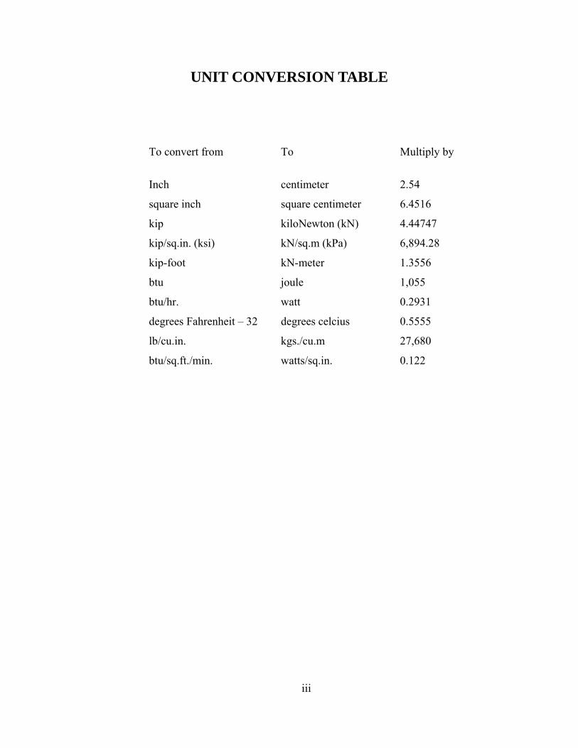
UNIT CONVERSION TABLE
To convert from To Multiply by
Inch centimeter 2.54
square inch square centimeter 6.4516
kip kiloNewton (kN) 4.44747
kip/sq.in. (ksi) kN/sq.m (kPa) 6,894.28
kip-foot kN-meter 1.3556
btu joule 1,055
btu/hr. watt 0.2931
degrees Fahrenheit – 32 degrees celcius 0.5555
lb/cu.in. kgs./cu.m 27,680
btu/sq.ft./min. watts/sq.in. 0.122

iv
Technical Report Documentation Page 1. Report No.
2. Government Accession No.
3. Recipient's Catalog No.
5. Report Date June 2007
4. Title and Subtitle
Integrative Information System Design for Florida Department of Transportation
A Framework for Structural Health Monitoring of Movable Bridges 6. Performing Organization Code UCF
7. Author(s) F. Necati Catbas, Melih Susoy, Ricardo Zaurin and Mustafa Gul
8. Performing Organization Report No.
10. Work Unit No. (TRAIS)
9. Performing Organization Name and Address University of Central Florida Civil and Environmental Engineering Department Engineering Bldg Room 211 Orlando, FL 32816
11. Contract or Grant No. BD548/RPWO 11
13. Type of Report and Period Covered Final Report November 2004 – April 2007
12. Sponsoring Agency Name and Address Florida Department of Transportation Research Center, MS 30 605 Suwannee Street Tallahassee, FL 32310
14. Sponsoring Agency Code FDOT
15. Supplementary Notes
16. Abstract Bridges constitute critical nodes of transportation systems, and therefore, ensuring their continuous operation is of utmost importance for safe and efficient transportation. Currently, visual inspections and simplified analysis techniques are employed for condition assessment and for decision making about bridges. A novel approach to bridge condition assessment is Structural Health Monitoring (SHM), defined as the measurement of operating and loading environment and critical responses of a system to track and evaluate incidents, anomalies, damage and deterioration. The objective of this project is to develop an SHM framework for integrative information system design. This framework is expected to improve bridge safety and to have efficient operation, effective and low cost maintenance by taking advantage of new technological advances. Movable bridges are considered as focus bridge type, because these bridges exhibit various structural, maintenance and operational problems. In this study, inspection and maintenance records of the movable bridges are analyzed to determine the current condition of these bridges as given in these reports. Then, numerical and experimental studies are developed and conducted. Data processing and some novel analysis methods that are being employed by the writers are summarized along with examples from laboratory studies. These analysis methods include statistical pattern recognition methods, parameter estimation with sensor fusion and model updating, estimation of reliability and prediction of future performance using Bayesian updating with monitor data, and possible use of computer vision. These algorithms have to be coupled with data monitoring front panels which can be used by engineers and other users. In this study, a data monitoring front panel, which makes it available to monitor multiple sensors is also developed and presented. Concepts for data management and use of information technologies for efficient and effective use of structural health monitoring data are discussed. Also, critical components and locations of movable bridges are summarized for monitoring purposes. In addition to structural components, Hopkins frame, trunnions, live load shoes, shafts, span locks electrical motors, gear boxes and open gears are determined to be candidates for monitoring. An application such as described in this report can be expected to mitigate the problems, improve future designs and reduce the maintenance costs. Further studies and field demonstrations are necessary to evaluate the real life performance of the technologies and methods as well as to quantify the cost-benefit ratio of integrated SHM applications.
17. Key Word Structural Health Monitoring, Movable bridges, sensors, data acquisition, data processing
18. Distribution Statement
19. Security Classif. (of this report) Unclassified
20. Security Classif. (of this page) Unclassified
21. No. of Pages 231
22. Price NA
Form DOT F 1700.7 (8-72) Reproduction of completed page authorized

v
ACKNOWLEDGEMENTS
This report is made possible through the support of the Florida Department of
Transportation (FDOT), and the guidance, suggestions and feedback of the FDOT central
office and district engineers. Messrs. Marcus Ansley, Angel Rodriguez, Richard Kerr and
Richard Long were very instrumental in the development of this project with their
continuous input. Especially, Mr. Marcus Ansley provided important feedback to develop
a monitoring framework throughout the project and also gave his review for the report.
Mr. Alberto Sardinas (from District 4) is to be acknowledged for sharing his experience
on movable bridges, and for making arrangements for site visits. District facilities
engineers Messrs. Ron Meade, Seta Koroitamoudou (from District 5) provided relevant
data, as well as shared their knowledge. Messrs. Lee Smith and Duane Robertson from
the FDOT Materials Laboratory at Gainesville provided valuable information about the
movable bridges. They are also acknowledged for conducting tests and providing the
data. Former graduate students Mr. Kevin Francoforte, Mr. Jason Burkett and Mr. Pavel
Babenko have been contributors to the development work presented in this report.

vi
PREFACE
The report describes and presents the background, methodology, and results of a
research project conducted by University of Central Florida researchers and funded by
the Florida Department of Transportation.

vii
EXECUTIVE SUMMARY
Background
Bridges constitute critical nodes of transportation systems, and therefore, ensuring
their continuous operation is of utmost importance for safe and efficient transportation.
Currently, visual inspections and simplified analysis techniques are employed for
condition assessment and for decision making about bridges. Despite limitations, visual
inspection remains today the most commonly practiced damage detection method. A
novel approach to bridge condition assessment is Structural Health Monitoring (SHM), or
more specifically Bridge Health Monitoring. SHM can be defined as the measurement of
a bridge’s operating and loading environment through use of a system to track and
evaluate incidents, anomalies, damage and deterioration. With a proper design, SHM is
expected to improve bridge evaluation and management techniques through
instrumentation, sensing, data processing, use of analytical methods, data evaluation
algorithms and data management. SHM utilizes advanced technology to capture the
critical inputs and responses of a structural system in order to understand the root causes
of problems as well as to track responses to predict future behavior.
Objective and Scope
The objective of this project is to develop a structural health monitoring
operational framework for an integrative information system design to improve bridge
safety, enhance efficiency and enable effective and low cost maintenance through use of
new technological advances. An integrative information system within an SHM
framework can facilitate information sharing and use by FDOT groups focusing on areas
such as structures, maintenance and operations that have similar data needs. While new
technologies offer promise, there are several issues that need further research. These are
a) managing data by means of methods and procedures developed for data collection, use
and evaluation, b) identification of critical features that need to be monitored for safety,

viii
maintenance and operation by means of statistical analysis, c) organization and use of the
most critical and desirable data and information for decision making, d) demonstration of
ideas and concepts.
In this project, a framework for different SHM applications has been developed
by identifying current issues affecting the maintenance of movable bridges and
conducting numerical and experimental studies. Movable bridges are considered “focus”
bridge types, because they exhibit various structural, maintenance and operational issues.
For example, movable bridges were reported to be about a hundred times more costly to
repair and maintain than fixed highway bridges because service includes not just
structural systems but also mechanical and electrical systems. Due to their significantly
higher cost of maintenance, increasing efficiency of movable bridge management
practices would have a higher benefit for monitoring demonstration purposes.
Project Tasks, Findings and Results
The first task of the project is the characterization of available data and user
needs. Common characteristics of Florida movable bridges and their distribution are
identified from the National Bridge Inventory (NBI). In addition, existing databases,
plans, inspection reports, and other relevant documents that were obtained from Districts
4 and 5 are analyzed to determine the most commonly observed movable bridge problem.
Site visits, meetings with FDOT officials and district engineers, and joint field tests
supplemented the data needed for understanding the condition of the bridges. A
representative bridge is also identified and its inspection and maintenance records are
analyzed over a 25-year period. The results of the analyses on the representative bridge
helped determine plans to address or remedy critical issues. Rapid deterioration due to
movements causing friction and wear of mechanical components, frequent and
unexpected breakdowns of components such as drive motors, shafts, gears, racks,
pinions, trunnions and limit switches require costly repair and maintenance. It is very
important to detect and even predict these failures in a timely manner to prevent
disruption to vehicular and marine traffic.

ix
The second task of the project is the development of monitoring strategies. After
the detailed evaluation of the inspection data of the representative bridge and
communication with FDOT engineers, finite element (FE) models of the bridge are
developed. The two different models which represent different levels of resolution are
both calibrated using field test data. The models are used to determine levels of stresses,
deflection under various load conditions. The tip deflection under single AASHTO HL-
93 truck and two HL-93 trucks+lane load are determined to be 1.65 in and 4.49 in,
respectively. The serviceability limit for this bridge and deck type is determined to be 5.6
in. The maximum stresses under dead load and two HL-93 trucks+lane load around
trunnion, at span lock and live load shoe are determined to be ~6-12 ksi, ~10 ksi, ~15 ksi,
respectively. The frequencies and mode shapes are also sensitive to damage, imbalance
and structural changes. For example, it is seen that additional modes appear when span
lock failure is simulated. For the undamaged condition, the first three modes are at 3.69
Hz, 4.74 Hz and 9.04 Hz. The load rating is determined to be lowest right above the love
load shoes. The inventory and operating rating values under two HL-93 trucks+lane load
at this location are 0.98 and 1.27, respectively. However, it is seen that under one HL-93
truck traveling at 50 mph, the lowest system reliability index is determined to be 5.79
which is far above the 3.5 (AASHTO LRFD for new design) and 2.5 (AASHTO LRFR
for existing bridges). These results are valuable to determine the monitoring locations,
sensing requirements and expected ranges.
The last task of the project is the design, implementation and demonstration of the
integrated framework. In this task, traditional and some novel sensors and sensor
networks are summarized along with criteria for the type and selection. Data acquisition
systems and communications are critical components of structural health monitoring
systems related with the acquisition of the data, including data collection, signal
processing, synchronization, digitization and storage. A data acquisition system is
proposed with different components and alternative data transmission protocols. In
addition, data transmission alternatives are offered for movable bridges. Data processing
and some novel analysis methods that are being developed by the writers are summarized
along with examples from laboratory studies. More specifically, statistical pattern

x
recognition methods, parameter estimation with sensor fusion and model updating,
estimation of reliability and prediction of future performance using Bayesian updating
with monitored data, and the possible use of computer vision approaches are presented
with examples. These algorithms have to be coupled with data monitoring front panels
which can be used by engineers and other users. It should be noted that three appendices
provide additional information about sensors, related laboratory studies and a brief
market search for sensing and data acquisition technologies. In this study, a data
monitoring front panel, which makes it available to monitor multiple sensors is also
developed and presented. Concepts for data management and use of information
technologies for efficient and effective use of structural health monitoring data are
discussed. Finally, critical components and locations for movable bridges are
summarized. In addition to structural components, Hopkins frame, trunnions, live load
shoes, shafts, span locks electrical motors, gear boxes and open gears are determined to
be candidates for monitoring.
Recommendations
Integrated structural health monitoring offers promise for improved condition
assessment and can complement current bridge management systems. An application
such as described in this report can be expected to mitigate both problems and
maintenance costs. Further studies and pilot applications are necessary to evaluate the
real life performance of technologies and methods as well as to quantify the cost-benefit
ratio of integrated SHM applications.
Finally, we note that the integrated monitoring framework proposed in this report
is developed in parallel to the efforts of the Federal Highway Administration Long Term
Bridge Performance Program (LTBPP), which focuses on continuous bridge monitoring
applications for developing improved knowledge on performance and degradation, better
design methods and performance predictive models, and advanced management decision-
making tools.

xi
TABLE OF CONTENTS
DISCLAIMER................................................................................................................... II
UNIT CONVERSION TABLE ...........................................................................................III
TECHNICAL REPORT DOCUMENTATION PAGE............................................................ IV
ACKNOWLEDGEMENTS.................................................................................................. V
PREFACE .......................................................................................................................VI
EXECUTIVE SUMMARY ................................................................................................VII
TABLE OF CONTENTS ...................................................................................................XI
LIST OF FIGURES ...................................................................................................... XVII
1. INTRODUCTION....................................................................................................... 1
1.1. Statement of the Problem................................................................................................ 1
1.1.1. Background of Bridge Inspections and Evaluations ..................................................... 2
1.1.2. New Technologies for Objective Bridge Assessment, Evaluation and Maintenance.... 3
1.2. Structural Health Monitoring as a Promising Approach............................................. 3
1.2.1. Definition ...................................................................................................................... 3
1.2.2. Components of a Complete SHM ................................................................................. 4
1.2.3. Promises of SHM.......................................................................................................... 5
1.3. Project Objectives and Goals .......................................................................................... 5

xii
1.4. Project Tasks .................................................................................................................... 6
1.4.1. Characterization of Available Data and User Needs..................................................... 6
1.4.2. Development of Monitoring Strategies ......................................................................... 7
1.4.3. Design, Implement and Demonstrate the Integrated Framework.................................. 7
2. CHARACTERIZATION AND ASSESSMENT OF BRIDGES ........................................... 8
2.1. Introduction...................................................................................................................... 8
2.2. Current Bridge Inspection and Management Procedure ............................................. 8
2.2.1. Bridge Inspection Program ........................................................................................... 8
2.2.2. Bridge Inspections in Florida ........................................................................................ 9
2.3. Issues for Today’s Bridge Management Practice........................................................ 11
2.3.1. Uncertainties in Condition Evaluation ........................................................................ 11
2.3.2. Asset Management ...................................................................................................... 11
2.3.3. Information Control .................................................................................................... 12
2.4. Characterization of Movable Bridges as Demonstration Example ........................... 13
2.4.1. Why Movable Bridges Selected as a Focus ................................................................ 13
2.4.2. Movable Bridges ......................................................................................................... 13
2.4.3. Status of Movable Bridge Population in Florida......................................................... 20
2.4.4. Compilation of Data from Maintenance Offices ......................................................... 22
3. MONITORING DEVELOPMENT STAGES ................................................................ 26
3.1. Introduction.................................................................................................................... 26
3.2. Site Visits and Meetings with FDOT Engineers – User Needs ................................... 26

xiii
3.3. Evaluation of Inspection Data....................................................................................... 28
3.3.1. Analysis of Inspection Data for a Subset Population .................................................. 28
3.3.2. Inspection Data Analysis for Christa McAuliffe Bridge over 30 Years...................... 33
3.4. Numerical Model Development for Analytical Evaluation of Structural Performance
38
3.4.1. Finite Element Model Development ........................................................................... 38
3.4.2. Initial Finite Element Model with Shell Elements ...................................................... 38
3.4.3. Modified Finite Element Model with Frame Elements ............................................... 47
3.5. Comparison of the Two Models.................................................................................... 51
3.6. Experimental Studies Conducted at the Bridge .......................................................... 54
3.6.1. Field Test Data Analysis (Balance Test) ..................................................................... 56
4. MODEL CALIBRATION, SIMULATIONS AND RATING............................................. 60
4.1. Introduction.................................................................................................................... 60
4.2. Calibration of the Model According to the Balance Condition.................................. 60
4.3. Analysis and Load Simulation Results......................................................................... 61
4.3.1. Loads Used for FE Simulations .................................................................................. 61
4.3.2. Deflections .................................................................................................................. 62
4.3.3. Stresses........................................................................................................................ 64
4.3.4. Dynamic Analysis ....................................................................................................... 67
4.3.5. Examples of Location for Monitoring Based on FEM................................................ 70
4.4. Movable Bridge Load Rating........................................................................................ 71

xiv
4.5. Moving Load Simulation............................................................................................... 76
4.6. Summary of Analysis Results ....................................................................................... 86
5. INTEGRATED STRUCTURAL HEALTH MONITORING DESIGN.............................. 90
5.1. Introduction.................................................................................................................... 90
5.2. Sensors And Sensor Networks ...................................................................................... 90
5.2.1. Traditional Sensors ..................................................................................................... 93
5.2.2. Some Novel Sensing Technologies............................................................................. 99
5.2.3. Wireless Sensing ....................................................................................................... 101
5.3. Data Acquisition Systems and Communication ........................................................ 102
5.4. Critical Components of Movable Bridges for Monitoring ....................................... 105
5.4.1. Electrical Motors....................................................................................................... 105
5.4.2. Gear Boxes................................................................................................................ 106
5.4.3. Open Gears / Racks................................................................................................... 107
5.4.4. Hopkins Frame.......................................................................................................... 111
5.4.5. Trunnions .................................................................................................................. 111
5.4.6. Live Load Shoes........................................................................................................ 115
5.4.7. Span Locks................................................................................................................ 116
5.4.8. Bridge Operation (Opening/Closing) ........................................................................ 118
5.4.9. Longitudinal Displacement ....................................................................................... 119
5.4.10. Main Girders and Floor Beams................................................................................ 119
5.5. Data Processing and Some New Analysis Methods................................................... 122

xv
5.5.1. Statistical Pattern Recognition .................................................................................. 125
5.5.2. Parameter Estimation with Sensor Fusion and Model Updating............................... 129
5.5.3. Estimation of Reliability using SHM Data................................................................ 133
5.5.4. Possible Use of Computer Vision Data for SHM...................................................... 141
5.6. Data Monitoring Front Panel...................................................................................... 145
5.7. Data Management and Information Technologies.................................................... 148
6. CONCLUSIONS AND RECOMMENDATIONS.......................................................... 151
7. REFERENCES....................................................................................................... 155
APPENDIX A. SENSORS AND DATA ACQUISITION SYSTEMS .............................. 162
A.1. Sensor Technology ....................................................................................................... 162
A.2. General Types of Sensors ............................................................................................ 162
A.3. Data Acquisition Systems Currently in Use at the UCF Structures and Systems
Research Laboratory................................................................................................................................ 168
A.3.1. VXI System .............................................................................................................. 168
A.3.2. National Instruments System .................................................................................... 169
A.3.3. Campbell Scientific................................................................................................... 170
A.3.4. Other Data Acquisition Systems ............................................................................... 171
APPENDIX B. RELATED LABORATORY STUDIES................................................ 173
APPENDIX C. INSTRUMENTATION COMPANIES AND MARKET SEARCH............ 192
A.1. Companies Related with SHM Sensor Development ................................................ 192
A.2. Sensors Market Search................................................................................................ 199

xvi
A.2.1. Accelerometer........................................................................................................... 199
A.2.2. Strain......................................................................................................................... 201
A.2.3. Temperature.............................................................................................................. 203
A.2.4. Tilt ............................................................................................................................ 203
A.2.5. Wireless Networking ................................................................................................ 204
A.2.6. Corrosion .................................................................................................................. 205

xvii
LIST OF FIGURES
Figure 2.1 – Movable bridge terminology (FDOT 2004) ............................................................................. 14
Figure 2.2 – Main types of movable bridges (Koglin 2003)......................................................................... 15
Figure 2.3 – Temporary bridge adjacent to the Bridge of Lions in open position (St. Augustine, FL) ........ 15
Figure 2.4 – Fort Denaud Swing Bridge, Florida ......................................................................................... 16
Figure 2.5 – A bascule bridge on the Miami River in Florida is open to let a ship pass (Buxton-Tetteh 2004)
............................................................................................................................................................ 17
Figure 2.6 – Florida DOT district map ......................................................................................................... 20
Figure 2.7 – Distribution of FDOT movable bridges ................................................................................... 21
Figure 2.8 – Distribution of FDOT movable bridges according to length of maximum span (NBI 2002)... 21
Figure 2.9 – Distribution of movable bridges according to year built (NBI 2002)....................................... 22
Figure 2.10 – Deterioration effects of corrosion on Michigan Street Bridge, Sturgeon Bay, Wisconsin
(Prine and Fish 1996).......................................................................................................................... 23
Figure 2.11 – Damage to Bridge to Sullivans Island, Charleston after hurricane Hugo, 1991 Source: NOAA
Photo Library (http://www.photolib.noaa.gov/historic/nws/wea00469.htm)...................................... 24
Figure 3.1 – Typical element condition from an inspection report............................................................... 29
Figure 3.2 – Analysis of inspection reports by creating spreadsheets from visual inspection data .............. 30
Figure 3.3 – Average condition states of components.................................................................................. 31
Figure 3.4 – Identification of common problems ......................................................................................... 31
Figure 3.5 – Most commonly observed movable bridge problems (District 4&5) ....................................... 32
Figure 3.6 – Case Study: Christa McAuliffe Bascule Bridge in Merritt Island, FL ..................................... 33

xviii
Figure 3.7 – Main girder of Christa McAuliffe Movable Bridge ................................................................. 34
Figure 3.8 – Christa McAuliffe Movable Bridge elevation.......................................................................... 34
Figure 3.9 – Christa McAuliffe Movable Bridge mechanical system .......................................................... 35
Figure 3.10 – Condition state: Decks ........................................................................................................... 36
Figure 3.11 – Condition state: Movable components ................................................................................... 36
Figure 3.12 – Condition state: Superstructure .............................................................................................. 37
Figure 3.13 – Condition state: Locks and live load shoes ............................................................................ 37
Figure 3.14 – 3D CAD model of the movable bridge .................................................................................. 39
Figure 3.15 – 3D CAD model; orthogonal views......................................................................................... 40
Figure 3.16 – Modeling of the bascule girder............................................................................................... 40
Figure 3.17 – Modeling of bascule girders with shell elements ................................................................... 41
Figure 3.18 – Detail of the pinned connection.............................................................................................. 41
Figure 3.19 – Model with shell elements (deck not shown) ......................................................................... 42
Figure 3.20 – Rigid links between frame elements ...................................................................................... 42
Figure 3.21 – Detail of the steel deck (Christa McAuliffe Bridge construction plans) ................................ 43
Figure 3.22 – Model of the real deck............................................................................................................ 43
Figure 3.23 – Deformations under load........................................................................................................ 44
Figure 3.24 – Deck modeled using 1.45 in thick steel shell element............................................................ 44
Figure 3.25 – Deflections under load ........................................................................................................... 45
Figure 3.26 – Connection of two spans ........................................................................................................ 46
Figure 3.27 – Finite element model with shell elements .............................................................................. 46

xix
Figure 3.28 – Modeling of bascule girders with frame elements.................................................................. 48
Figure 3.29 – Main girders, transverse girders, floor beams, and bracings. ................................................. 48
Figure 3.30 – Close-up on the trunnion in the modified model.................................................................... 49
Figure 3.31 – Supports (boundary conditions) of the model (deck not shown)............................................ 49
Figure 3.32 – Completed modified FEM (Deck not shown). ....................................................................... 50
Figure 3.33 – Analysis details for the modified FEM .................................................................................. 50
Figure 3.34 – Load case studied for model comparison ............................................................................... 51
Figure 3.35 – Finite element models deflection comparison........................................................................ 52
Figure 3.36 – Comparison of the first three principal modes ....................................................................... 53
Figure 3.37 – Desirable Balance Condition of a Bascule Bridge ................................................................. 54
Figure 3.38 – Different cases of average torque during opening and closing............................................... 55
Figure 3.39 – Balance test results for March 2003 ....................................................................................... 57
Figure 3.40 – Balance test results for February 2003 ................................................................................... 57
Figure 3.41 – Balance test results for February 2006 ................................................................................... 58
Figure 3.42 – Change of friction values ....................................................................................................... 59
Figure 4.1 – Balance condition of the leaves................................................................................................ 61
Figure 4.2 – HL-93 truck load ...................................................................................................................... 61
Figure 4.3 – Loading for load rating of the bridge (Two HL-93 trucks and distributed lane load) .............. 62
Figure 4.4 – Deflections at the center. .......................................................................................................... 63
Figure 4.5 – Von Mises stresses for Dead Load (ksi)................................................................................... 64
Figure 4.6 – Von Mises stresses for Truck Load (ksi).................................................................................. 65

xx
Figure 4.7 – Von Mises stresses for Dead Load and Truck Load (ksi) ........................................................ 65
Figure 4.8 – Von Mises stresses at the THG connection for Dead Load (ksi) ............................................. 65
Figure 4.9 – Von Mises stresses at the THG connection for Truck Load (ksi) ............................................ 66
Figure 4.10 – Von Mises stresses at the THG connection for Dead Load and Truck Load (ksi) ................. 66
Figure 4.11 – Modal analysis results: Mode 1.............................................................................................. 67
Figure 4.12 – Modal analysis results: Mode 2.............................................................................................. 68
Figure 4.13 – Modal analysis results: Mode 3.............................................................................................. 68
Figure 4.14 – Modal analysis results: Mode 4.............................................................................................. 68
Figure 4.15 – Modal analysis results: Mode 5.............................................................................................. 69
Figure 4.16 – Modal analysis results: Mode 6.............................................................................................. 69
Figure 4.17 – Additional mode shapes for a span-lock failure scenario....................................................... 70
Figure 4.18 – Span lock failure simulation................................................................................................... 71
Figure 4.19 – Transverse loading ................................................................................................................. 72
Figure 4.20 – Truck position for load rating (lane load not shown) ............................................................. 72
Figure 4.21 – Section locations for load rating............................................................................................. 73
Figure 4.22 – Moving Load Analysis ........................................................................................................... 76
Figure 4.23 – Variation of Moment due to Moving Load over the Girder Locations .................................. 77
Figure 4.24 – Section properties of Section 1 along the girder .................................................................... 79
Figure 4.25 – Section properties of Section 2 along the girder .................................................................... 79
Figure 4.26 – Section properties of Section 3 along the girder .................................................................... 80
Figure 4.27 – Movable Bridge System Reliability Model with Parallel/Series Assembly (Lower Bound) . 84

xxi
Figure 4.28 – Instantaneous System Reliability under a Single Moving Truck (note that this is for one
moving truck without lane load, wind, temperature) .......................................................................... 85
Figure 4.29 – Loading position for ............................................................................................................... 86
Figure 5.1 – Example foil type strain gages (Omega Eng.).......................................................................... 94
Figure 5.2 – Example vibrating-wire type strain gages (Geokon Inc.)......................................................... 95
Figure 5.3 – Displacement gage examples (Spaceage Control).................................................................... 96
Figure 5.4 – Tiltmeter examples (Applied Geomechanics, Geokon) ........................................................... 97
Figure 5.5 – Example accelerometers (PCB) ............................................................................................... 97
Figure 5.6 – An example wind station for measuring wind direction, speed and temperature (Omega Inc.)98
Figure 5.7 – Sensor array + DAQ scheme.................................................................................................. 103
Figure 5.8 – Data transmission with two data acquisition systems via under-water cable ......................... 104
Figure 5.9 - Data transmission with two data acquisition systems via wireless connection....................... 104
Figure 5.10 – Data transmission with wireless sensor array....................................................................... 105
Figure 5.11. Some of the proposed metrics for Level 1 monitoring (raw data indicators) ......................... 124
Figure 5.12. Pattern classifier (adapted from Webb 1999)......................................................................... 125
Figure 5.13 – Supervised and unsupervised learning for SHM .................................................................. 126
Figure 5.14. Some of the proposed metrics for Level 2 monitoring (identification of damage) ................ 127
Figure 5.15 – Mahalanobis distance plots to detect damage case............................................................... 129
Figure 5.16. Some of the proposed metrics for Level 3 monitoring (quantification and localization) ....... 130
Figure 5.17 –General methodology for parameter estimation and model updating.................................... 132
Figure 5.18 –Estimation of the stiffness parameters at the supports with statistical bounds ...................... 133

xxii
Figure 5.19 – Limit state functions (Nowak and Collins 2000).................................................................. 135
Figure 5.20 – Concept of Bayesian Updating............................................................................................. 136
Figure 5.21 – Simple beam test for Bayesian updating demonstration ...................................................... 138
Figure 5.22 – Test beam ............................................................................................................................. 138
Figure 5.23 – Prior and new data for the test beam .................................................................................... 139
Figure 5.24 – Updating the available data and prediction with the first data set using Bayesian............... 140
Figure 5.25 – Reliability based on SHM data............................................................................................. 141
Figure 5.26 – Computer vision integration into SHM................................................................................ 142
Figure 5.27 – Data monitoring for the laboratory health monitoring setup ................................................ 146
Figure 5.28 – Movable bridge remote monitoring system.......................................................................... 147
Figure 5.29 - Database implementation...................................................................................................... 148
Figure 5.30 - Database functional layers .................................................................................................... 149
Figure 5.31 – Example framework for internet-based database ................................................................. 150
Figure 5.32 – Electrical motor.................................................................................................................... 106
Figure 5.33 – A gear box............................................................................................................................ 107
Figure 5.34 – Open gear / rack ................................................................................................................... 108
Figure 5.35 – Rack details (Patton 2006) ................................................................................................... 108
Figure 5.36 – Area for searching is defined ............................................................................................... 110
Figure 5.37 – Histogram of the pixel intensities and determination of interest regions ............................. 110
Figure 5.38 – Detection of corrosion/indentation....................................................................................... 110
Figure 5.39 – Hopkins frame girder ........................................................................................................... 111

xxiii
Figure 5.40 – Trunnion............................................................................................................................... 112
Figure 5.41 – Instrumentation for the mechanical components (Adapted from Christa McAuliffe Bridge
Construction Plans)........................................................................................................................... 113
Figure 5.42 – Instrumentation of mechanical components......................................................................... 114
Figure 5.43 – Mechanical system of the representative movable bridge (Adapted from Christa McAuliffe
Bridge Construction Plans) ............................................................................................................... 115
Figure 5.44 – Live load shoe (LLS) (sketch adapted from Christa McAuliffe Bridge construction plans) 116
Figure 5.45 – Span lock.............................................................................................................................. 117
Figure 5.46 – Instrumentation for the span lock (Adapted from Christa McAuliffe Bridge construction
plans)................................................................................................................................................. 117
Figure 5.47 – Opening/closing of the leaf .................................................................................................. 118
Figure 5.48 – Main girders in open position............................................................................................... 120
Figure 5.49 – Possible instrumentation for movable bridge structural components................................... 121
Figure A.1 – A strain rosette ...................................................................................................................... 163
Figure A.2 – Signal conditioning ............................................................................................................... 169
Figure A.3 – National Instruments system in the laboratory; (a) SCXI 1001 chassis, (b) PXI 1033 chassis
.......................................................................................................................................................... 170
Figure A.5 – Microstrain data acquisition and transmitter ......................................................................... 172
Figure B.1 – Test beam .............................................................................................................................. 173
Figure B.2 – Some tests performed on the test structure ............................................................................ 174
Figure B.3 – Analysis results from the instrumented beam........................................................................ 174
Figure B.4 – Grid structure in the laboratory ............................................................................................. 175
Figure B.5 – Results of dynamic analysis and damage scenarios............................................................... 175

xxiv
Figure B.6 – General Methodology............................................................................................................ 177
Figure B.7 – Test setup............................................................................................................................... 181
Figure B.8 – Example pictures showing different BC (a) The pin support for BC1 (b) Four Duro50 pads
for BC2 (c) Five Duro70 pads for BC4............................................................................................. 183
Figure B.9 – Time history data (a) Ambient data (b) Data after averaging with RD plotted with the data
estimated with AR (c) A closer look at the figure in (b) ................................................................... 184
Figure B.10 – Analysis results for BC1, BC2 and BC3 (a) Mahalanobis distance of the AR coefficients for
BC1 and BC2 (b) Clustering of the AR coefficients for BC1 and BC2 (c) Mahalanobis distance of the
AR coefficients for BC1 and BC3 (d) Clustering of the AR coefficients for BC1 and BC3 (each point
in the figures is coming from one data block)................................................................................... 186
Figure B.11 – Mahalanobis distance of the AR coefficients f for BC1, BC3 and BC4 (each point in the
figures is coming from one data block)............................................................................................. 187
Figure B.12 – The physical grid model and test setup................................................................................ 188
Figure B.13 – Damage scenarios applied to the steel grid.......................................................................... 188
Figure B.14 – Determining the threshold value for the grid....................................................................... 189
Figure B.15 – Mahalanobis distance plots for scour case........................................................................... 190
Figure B.16 – Mahalanobis distance plots for restraint supports................................................................ 190
Figure B.17 – Mahalanobis distance plots for reduced stiffness ................................................................ 191

1
1. INTRODUCTION
1.1. STATEMENT OF THE PROBLEM
Bridges constitute critical nodes of transportation systems, and therefore, ensuring
their continuous operation is of utmost importance for safe and efficient transportation.
Deterioration due to environmental effects and operational loading causes bridge
performance to decline, and may even result in collapse. The U.S. requires periodic
bridge inspections, which should then be reported to the Federal Highway Administration
(FHWA) through the National Bridge Inventory Standards (NBIS). These inspections,
however, are mainly based on subjective visual inspections, while a thorough
understanding of the performance and behavior of a bridge requires extensive analysis,
modeling and test results.
Load rating is another method used for decision making, traffic operations, load
posting and issuing permits. Load rating of bridges as described by AASHTO Manual for
Condition Evaluation and Load and Resistance Factor Rating (LRFR) of Highway
Bridges (2003b) is employed for more in-depth bridge evaluation practices based on
numerical models and available data on the specific bridge. Bridges may be rated
according to this procedure for inventory rating if the safety is of concern, or for
operating rating if a special load permit is requested. Load rating analysis is generally
conducted using simplified software such as BAR7 (PennDOT 2001). Using more
accurate analytical model and assumptions in the load rating calculation will result in
more dependable evaluation results (Catbas et al. 2005).
Highly developed analysis techniques, such as linear and nonlinear finite element
modeling, can be used to simulate the structural response. Complex boundary conditions,
material behavior, interactions between substructural components, and time-dependent
effects have to be estimated through certain assumptions, which hinder the reliability of
the model. In case of a complex, irregular, or extraordinary structure, destructive or
nondestructive tests may be necessary to calculate the actual capacity, or required
parameters, or to calibrate/validate the model. Destructive load tests, while precise,

2
cannot be carried out for in-service evaluation of structures. Therefore, condition
assessment must be based on data obtained through non-destructive testing methods.
A Structural Health Monitoring (SHM) application is an integrated system formed
by the collection of efforts aiming to advance decision-making. SHM can use continuous
or intermittent structural monitoring via sensors. Key parameters are determined by
employing analysis techniques to indicate the condition and performance of the bridge.
The sophistication of SHM differs widely according to the needs and characteristics of
each application. Currently, SHM is used primarily for major bridges, demonstration
studies or bridges showing signs of critical distress. However, FHWA has been
developing and coordinating the new Long Term Bridge Performance (LTBP) program
for the implementation of SHM in a more effective manner and eventually for the
development of guidelines.
While new technologies within the context of SHM exist, there is a strong need
for defining an integrated approach to link data collection, evaluation techniques and
efficient data management. There also needs to be a unified approach with guidelines and
standards to provide consistency in bridge data collection and evaluation, so that
objective comparisons for decision-making can be conducted. This is possible through an
integrated SHM approach.
1.1.1. Background of Bridge Inspections and Evaluations
Visual inspection is the traditional method for damage detections. However, this
method has some inherent drawbacks, the first of which is the damage must have
progressed far enough to be visually observable. Second, visual inspection is inherently
subjective not just for identifying the implication of damage but also in the detection of
damage. A study conducted by the Federal Highway Administration’s NDE Center on the
accuracy of visual inspection of short-to-medium span bridges concluded that at least
56% of the bridges given an average condition rating were done incorrectly (Turner-
Fairbank Research Center 2005). Even if the damage is successfully identified, the final
problem facing the engineer is accurately assessing its effect on the overall “health” of

3
the structure (Aktan et al. 2001b). Visual inspection also requires much time and effort,
and may overlook locations of limited and/or no accessibility.
For extended structures, such as long-span suspension bridges, the difficulty is
further compounded. Successful visual inspection of these structures is dependent on
inspecting all possible damage scenarios at all critical locations, not an easily
accomplished task even for an experienced inspector (Aktan et al. 2001a). Despite all
these limitations, visual inspection remains today the most commonly practiced damage
detection method.
1.1.2. New Technologies for Objective Bridge Assessment, Evaluation and
Maintenance
The state-of-the-art in SHM allows for advanced techniques with sensing devices
and analysis methods to be used to capture and quantify parameters of concern. These
technologies show great promise for complementing and improving current inspection
techniques. However, these novel methods also introduce various challenges to the bridge
engineer, such as evaluation of large amounts of data in a timely manner. Without proper
guidance and established standards, jobs such as sensory systems application, data
collection and analysis could prove to be a burden for the bridge engineer.
The growing availability of sensors and sensing technologies is making it even
easier to implement instrumentation applications on as large a scale as needed. Therefore,
the main challenge is not collecting data, but making sense of it. A successful SHM needs
evaluation of data into useful information in a timely manner.
1.2. STRUCTURAL HEALTH MONITORING AS A PROMISING APPROACH
1.2.1. Definition
Structural Health Monitoring, or SHM, is defined as the measurement of
operating and loading environments and critical responses of a system to track and
evaluate incidents, anomalies, damage and deterioration. With a proper design, SHM is
expected to advance bridge evaluation and management approach through

4
instrumentation, sensing, data processing, use of analytical methods, data evaluation
algorithms and data management techniques, at the project level as well as the network
level. SHM utilizes advanced technology to capture the critical inputs and responses of a
structural system with various types of sensors and analysis methods as part of the health
monitoring framework to understand the root causes of the problem as well as to track
responses to predict future behavior.
1.2.2. Components of a Complete SHM
A complete SHM application is created by many interacting components, which
may be added or subtracted according to the specific needs of each application, but the
main categories may be broadly summarized as follows (Catbas et al. 2004);
Experimental Components: Include the selection of sensory devices,
instrumentation locations, measurement types, and tests, such as static, dynamic or
localized non-destructive testing. General categories can be listed as geometry
monitoring, controlled testing (which may be static or dynamic, nondestructive or
destructive) and continuous monitoring. Acquiring data from the sensor devices, signal
conditioning, and transferring the data to main terminals is part of the data acquisition
component. Data acquisition systems provide the excitation, initial filtering, collection
and analog-to-digital conversion of the signals as well as storage in the appropriate
format.
Analytical Components: Composed of all analysis tools necessary for extracting
the required information from the data. Analytical components may be drafting, modeling
and structural analysis techniques along with the instrumentation, as well as data
processing and algorithms such as statistical pattern recognition or parameter
identification. Without proper analysis techniques, we cannot expect to generate useful
information from acquired sensor data.
Information Technology: Represents all the methods and framework through
which the information is stored, managed and shared. A successful IT application also
provides access to the information through visualization and user interfaces. This is a key

5
component of SHM applications by providing the backbone and their design vary widely
according to the requirements of the application.
1.2.3. Promises of SHM
With recent rapid developments in electronics and communications, sensor
technologies have developed such that costs are reduced, accuracies are improved and
novel approaches such as wireless sensing, fiber-optic sensors, MEMS
(microelectromechanics) sensors, distributed networking and internet-based data
acquisition are introduced. Now it is more feasible to acquire data about the status of
structural responses, such as strain, displacement, vibration, and environmental effects,
such as wind speed, temperature and earthquake excitation. For an effective
implementation, it is important to integrate novel experimental technologies, analytical
methods and information technologies for determining the structural condition. SHM
offers accurate information and detection of distress that visual inspections cannot reveal.
SHM can be employed for obtaining global and local structural parameters, data for
structural identification (geometric/ FE model calibration), effective maintenance and
operation. It can also be used for improving future designs. Diagnosing pre- & post-
hazard conditions for emergency management can also be facilitated by SHM.
1.3. PROJECT OBJECTIVES AND GOALS
The ultimate objective of the project is to develop an SHM framework for
integrative information system design to enable FDOT to improve practices and provide
the best possible transportation infrastructure by taking advantage of new technological
advances. In order to develop an integration information system, three groups within
FDOT (structures, maintenance, operations) were identified that would have similar data
needs and could provide feedback and guidance. A kick-off meeting with structures,
maintenance and operations engineers was held in Tallahassee. Based on the valuable
feedback that was received during the kick-off meeting and other subsequent meetings
and communications, the initial scope of the project was revised approximately six
months after the start. New objectives include:

6
Managing data effectively and efficiently. Development of policies and approaches for
consistent structural health monitoring applications within the organizations for
mitigation of possible problems inconsistencies for data collection, sharing and data
comparing within each FDOT district.
Identifying critical features that need to be monitored for safety, maintenance and
operation. Development of monitoring strategies based on statistical information
extracted from the data and engineering heuristics.
Organizing the most critical and desirable data and information. It is known that
statistical tools could be made available to approximate the current condition,
provided that the data is well organized. Efficient storage, organization and
availability of the data would make it possible to plan ahead.
Demonstrating the ideas and concepts of this study by integrating data and information
for the movable bridges.
As a result, the main goal of the current project is to develop an SHM framework
that will serve the different users of FDOT for bridge management and operations within
an Integrative Information System context. The first goal of the project is: To identify the
challenges and inefficiencies in bridge monitoring, data management and information
control procedures to improve and supplement current bridge management methods by
establishing a general SHM framework that can be employed by different districts and
offices. Another major goal will be to provide guidelines, standards and a demonstration
study for future applications that can be carried in a more uniform manner with all critical
components of SHM taken into consideration. The project focuses on exploring the use of
advanced information technology demonstrations for movable bridges as a case study.
1.4. PROJECT TASKS
1.4.1. Characterization of Available Data and User Needs
Characterize interacting systems with all the critical parameters affecting component
and individual system performances.
Characterize data needs, existing data, information and knowledge available in the
existing FDOT databases. Communicate with FDOT engineers on the preliminary

7
design of the integrated system for legacy as well as new and objective field data to be
collected. Collect and analyze FDOT’s existing data and information assets, which
exist in a variety of databases and in hard-copy formats, with the specific focus on the
movable bridges.
Identify and collect data/information such as the inspection and maintenance reports,
analytical and experimental data for existing condition evaluation and load rating
reports by closely working with structures, maintenance and operations engineers.
1.4.2. Development of Monitoring Strategies
Investigate and identify the critical features that need to be monitored for safety,
maintenance and operation to enable successful development of monitoring strategies
based on statistical information extracted from the data and engineering heuristics.
Investigate and define the sensing and data acquisition and other related hardware for
possible standardized structural health monitoring practices.
Conduct benchmark tests and evaluation studies in the laboratory in order to
exemplify the application of the structural health monitoring hardware components.
1.4.3. Design, Implement and Demonstrate the Integrated Framework
Design, implement and demonstrate a framework that will use the state-of-the-art
approaches for collecting and analyzing data to generate valuable and useable
information and knowledge for decision making. The system will include data and
information for the selected movable bridges. Possible monitoring designs will be
developed in such a way that the most critical and desirable data and information
about movable bridges can be generated, analyzed timely and utilized to help decision
making for maintenance, structural repairs and operations. In addition, the PI and his
students will investigate the use of statistical tools that can be embedded in the
integrated SHM framework to approximate the current condition. Efficient storage,
organization and easy and timely availability of the data are important issues for a
complete SHM framework.

8
2. CHARACTERIZATION AND ASSESSMENT OF BRIDGES
2.1. INTRODUCTION
In order to address the issues related to decision making for bridge management
and accomplish the project tasks, it is important to review the current condition of bridges
and bridge management practice in the nation and in Florida. First, the current approach
for bridge inspection and decision-making process was investigated. Then the movable
bridge population was evaluated with this understanding. General characteristics of the
movable bridges in terms of the main parameters such as geometry, type and condition
were analyzed and summarized.
2.2. CURRENT BRIDGE INSPECTION AND MANAGEMENT PROCEDURE
2.2.1. Bridge Inspection Program
The National Bridge Inspection Standards (NBIS) applies to all structures defined
as bridges located on all public roads. In accordance with the AASHTO (American
Association of State Highway and Transportation Officials) Transportation Glossary, a
“bridge” is defined as a structure including supports erected over a depression or an
obstruction, such as water, highway, or railway, and having a track or passageway for
carrying traffic or other moving loads, and having an opening measured along the center
of the roadway of more than 6.1 m (20 feet). These openings are between undercopings
of abutments or spring lines of arches, or extreme ends of openings for multiple boxes. A
bridge may also include multiple pipes, where the clear distance between openings is less
than half of the smaller contiguous opening.
NBIS regulates that each highway department shall include a bridge inspection
organization capable of performing inspections, preparing reports, and determining
ratings in accordance with the Manual for Condition Evaluation of Bridges (AASHTO
2003a). Inspection records and bridge inventories are to be prepared and maintained.
According to NBIS, location, description, inspection frequency and procedures
for fracture critical members (members of a bridge whose failure will probably cause a

9
portion of or the entire bridge to collapse), underwater members and special features are
to be listed for each bridge, with their previous inspection dates. Each bridge is to be
inspected at regular intervals not to exceed two years, or less depending on such factors
as age, traffic characteristics, state of maintenance, and known deficiencies. The
inspections are conducted by a team of qualified personnel. In order to qualify as an
inspector, professional engineer registration or a minimum 10 years of experience in
bridge inspection assignments is needed together with the completion of the
comprehensive training course (AASHTO 1983).
2.2.2. Bridge Inspections in Florida
The findings and results of bridge inspection are recorded on standard forms.
These inspection reports have to be kept by the state DOTs and reported to the FHWA in
required formats. For many states, including Florida, inspection data are stored and used
by means of software such as PONTIS or BRIDGIT. Each state prepares and maintains
an inventory of all bridge structures. Inventory and appraisal data must be collected and
retained within the various departments of the state organization for collection by the
Federal Highway Administration as needed. A tabulation of this data is contained in the
structure inventory and appraisal sheet distributed by the Federal Highway
Administration (FHWA 1995).
Florida Department of Transportation (FDOT) inspectors must be either state-
licensed professional engineers or they must complete the National Highway Institute
course in bridge inspection and meet FDOT's experience requirements (FHWA 2003).
FDOT's development program classifies the inspectors’ recommendations into three
categories:
Routine maintenance
Periodic maintenance and repair
Replacements
Once the inspectors' recommendations are sorted into the three categories above,
the next step is to create work orders. Work orders are given priority ratings from 1 to 4,

10
priority 1 being an emergency situation requiring work to be completed within 60 days;
priority 2, an urgent situation with a 180-day limitation; priority 3, routine work to be
done within 1 year; and priority 4, no immediate deadline but information is provided.
All work orders are scheduled and performed by the districts or by an independent asset
management contractor (FHWA 2005).
FDOT has implemented PONTIS, a Bridge Management System, to provide
decision support to engineers in the headquarters and district offices as they make routine
policy, programming, and budgeting decisions regarding the preservation and
improvement of the state’s bridges. A Feasible Action Review Committee (FARC) in
each district office is responsible for reviewing and prioritizing the needs identified by
the inspectors. FARC uses the Project-Level Analysis Tool (PLAT), an integrated
software customized for FDOT. PLAT is a project-level decision support framework that
complements and builds on PONTIS’ existing network-level analysis. Specific models
include:
Accident risk and user cost due to roadway width and alignment deficiencies
User cost of load capacity, vertical clearance restrictions, and movable bridge
openings
Project-level prediction models for bridge element conditions and costs
Prediction of economics of scale and scoping possibilities.
These new PLAT models are displayed graphically in a spreadsheet format as an
aid in decision making. Engineers use PLAT to determine the economic health of a
structure, and they use it as a design tool for candidate projects to program into the
management process. When the engineer modifies a candidate by changing the element
action selections, quantities, or various cost factors, PLAT responds, immediately
updating its predictive results. This new project-level decision support framework
complements and builds on the existing network-level analysis in PONTIS. Florida is one
of the few States integrating PONTIS to do network-level analysis applications
(Thompson et al. 2003; FHWA 2005).

11
2.3. ISSUES FOR TODAY’S BRIDGE MANAGEMENT PRACTICE
2.3.1. Uncertainties in Condition Evaluation
The ability to monitor the condition of a bridge structure to capture the structural
parameters or changes in condition is of significant interest to many bridge owners.
Traditionally, visual inspections have been used. Inspectors follow a scheduled plan,
every two years in most cases, to identify which bridges need preventative maintenance,
minor or major repair work, or replacement. A bridge that meets the standards is defined
as not showing evidence of structural deterioration, not being limited by weight
restrictions or not needing preventative maintenance. One big problem with this
subjective approach is that if damage occurs gradually, it may not be observed by
inspectors. If access to some parts is difficult, observations are done from a distance and
are not always accurate. Shortcomings of visual inspections are well-documented in a
study by FHWA Turner-Fairbank Research Center (Turner-Fairbank 2005). Unless great
damage is present, no inspection will be done outside of the scheduled plan. Even if the
damage is successfully identified, the final problem facing the engineer is accurately
assessing its effect on the overall health of the structure (Aktan et al. 2001b).
Obviously, the major issue is not obtaining measurements, but rather how to
process, analyze and convert the data into useful information about the condition and
performance of the bridges. In addition, it is important to provide the bridge owners with
the future performance predictions for decision making such as condition-based
maintenance scheduling.
2.3.2. Asset Management
The task of maintaining a large bridge population in good condition requires
considerable effort and budget. In addition to that, the fact that the bridge population is
aging means ever-increasing costs for maintenance. State departments of transportation
and districts allocate a certain proportion of their total budget to preservation. The
available maintenance budget should be allocated to routine maintenance and retrofitting
a portion of bridges showing deficiency. To determine funding priorities, network-level

12
analysis needs to be carried out. The analysis should consider the total cost-benefit trade-
off, which requires both detailed structural condition analysis and condition predictions
for alternative actions. Decisions based merely on condition ratings and simplified
structural analyses with high uncertainty would not be efficient. Objective assessment of
the condition using new, cost-effective technologies and condition-based maintenance is
becoming crucial.
2.3.3. Information Control
The information generated by districts are used by FDOT Headquarters for
maintenance, repair prioritization and resource allocation. Information obtained by
different offices in the DOT and districts over different counties can be incompatible, due
to insufficient standardization of data collection and management. Bridge inspection and
maintenance data are kept with PONTIS software, commonly adopted in Florida.
However, this information is localized and each district manages its own inspection
results. Since ownership and responsibility of data collection and collected data are the
responsibility of independent districts, that may result in inconsistencies and
inefficiencies in managing the data by FDOT headquarters.
Information management is the key for efficient transportation asset management.
Information related to condition and operation of highway bridges are required by
numerous branches of state departments of transportation. For example, bridge
performance information is to be used by the maintenance office for monitoring the
performance and planning repair and rehabilitation operations. The structural design
office needs the same information to derive and validate data for modeling and analysis.
The division associated with traffic operations needs certain data related with bridge
usage, which is also of concern for structures and maintenance groups. Lack of
communication and information exchange between these offices may be a major problem
causing collection of duplicate data or delays. Similarly, an SHM design should also
recognize these challenges and provide a standardized platform for applications by
various users.

13
2.4. CHARACTERIZATION OF MOVABLE BRIDGES AS DEMONSTRATION EXAMPLE
2.4.1. Why Movable Bridges Selected as a Focus
The Florida Department of Transportation (FDOT) bridge inventory includes a
large number of movable bridges. For the current research project, the movable bridges
were chosen due largely based upon the following distinctions:
High maintenance cost of movable bridges (the average maintenance cost is about 100
times that of fixed bridges per square ft)
Frequency of breakdowns due to the high number of movable parts
Malfunctions cause not only problems in land traffic, but also marine traffic
Difficulties in determining the root cause(s) of breakdown and predicting future
breakdowns
As a result, FDOT engineers indicated that the movable bridges would provide a
better demonstration case, while improvements through the conducted study will have
more significant benefits.
2.4.2. Movable Bridges
2.4.2.1 Definition of a Movable Bridge
A movable bridge is a structure which has movable components operated by
various types of machinery to open the passageway for maritime traffic. Movable bridges
are employed when the vertical clearance of the bridge carrying the roadway/pedestrian
way over a river, canal or any water body is not sufficient for the vessels traveling over
the waterway. A movable bridge is a viable alternative to a high fixed bridge over the
waterway, however, they also contain significant drawbacks and problems, which are to
be mentioned specifically in the following sections. In certain cases, where aesthetics and
dimensional constraints dominate the design, movable bridges constitute the only choice.

14
2.4.2.2 Movable Bridge Terminology
Although highly variable in type, configuration and geometry, common
terminology and features for movable bridges are shown given in Figure 2.1. Movable
bridges have approach spans, movable spans, operator room, machinery room, traffic
gates and span locks. Typically, they are over a channel or a similar waterway. Fenders
are often installed to protect the piers.
Figure 2.1 – Movable bridge terminology (FDOT 2004)
Although this schematic is for the most common type, there are several kinds of
movable bridges. Three main types are shown in Figure 2.2, which are to be explained in
detail in the following section.

15
Figure 2.2 – Main types of movable bridges (Koglin 2003)
2.4.2.3 Types of Movable Bridges
Lift Type Bridge
Vertical lift bridges use cables, pulleys, motors and counterweights to raise a
section of the bridge vertically. The classical lifting bridge is used in urban areas with
scarce space for bridging inland waterways. Overhead clearance for navigation is limited,
however, these bridges have the advantage over bascule bridges in that they can be made
of any length feasible for a simple span. Disadvantages are a high initial cost and
expensive operation (Buxton-Tetteh 2004). The temporary lift bridge shown in Figure 2.3
is a typical example for lift type movable bridges.
Figure 2.3 – Temporary bridge adjacent to the Bridge of Lions in open position (St. Augustine, FL)

16
Swing Type Bridges
Swing bridges rotate their spans on a pedestal, allowing vessels to move past on
either side. The swing bridge over the Caloosahatchee River, Florida (Figure 2.4) is an
example of a pedestal type swing bridge. Swing bridges do not move vertically, therefore,
operation is easier. However, the pedestal is usually located in the middle of the channel,
creating a navigation hazard.
Figure 2.4 – Fort Denaud Swing Bridge, Florida
Bascule Type Bridges
A bascule bridge is a drawbridge with a counterweight that continuously balances
the span, or "leaf", throughout the entire upward swing in providing clearance for boat
traffic.
Bascule bridges have interior spans called "leaves" that rotate upward and away
from the centerline of the river, providing clear passage for river traffic. Unlike the
vertical lift bridges, when opened, there is no vertical obstacle to river traffic. They rotate
about trunnions or roll back on circular segments, or have a combined motion of turning

17
and rolling, and are counterweighted to reduce the power required for operation. There
are motors that turn the reduction gears connected to shafts and gears. These gears are
connected to rack assemblies, which are mounted on the counterweights. Bascule bridges
are made in one leaf, or in two leaves that meet in the center. The two-leaf bridges have a
locking device at the ends, and are arranged to act as cantilevers when closed, and
sometimes as three-hinged arches. The span locks keep the ends of the leaves from
bouncing as traffic passes over them.
Bascule bridges with one leaf or symmetrical bascule bridges with two leaves
have an opening angle of up to 85° to create optimum clearance for navigation without
upper limitation. In case of navigation channels near the coast which are also used by
large deep-sea vessels bascule bridges are particularly appropriate because they offer
unlimited overhead clearance and their large spans are able to cope with wide shipping
channels. In urban areas with scarcity of space and no possibility of high access for cross
traffic, bascule bridges offer a solution for the "crossing" of road and waterborne traffic
(Koglin 2003).
Figure 2.5 – A bascule bridge on the Miami River in Florida is open to let a ship pass (Buxton-Tetteh 2004)

18
2.4.2.4 Movable Bridge Inspections
Movable bridges are subject to regular NBI inspections, as well as underwater
inspections. Regular inspections have been expanded to cover mechanical, electrical and
other special components, which are also rated according to similar guides. Inspection
procedures for some movable bridge elements are summarized as example.
Open gearings: Alignment and wear of open gearings are inspected. Grease
patterns are checked for signs of misalignment and tooth surface is inspected for
deterioration and cracks. If present, proper alignment of pitch-lines is checked.
Enclosed gearings: Alignment and wear is also a major concern for enclosed
gearings. The gearing is visually inspected through inspection ports, reducer supports are
examined for cracks or deterioration, bolting is checked for tightness. Also checked are
the oil level, leaks on the box and seals. Operating sounds are checked for abnormal
noises. Oil sample is taken from bottom of box for chemical analysis.
Bearings: There are different inspection procedures for different types of
bearings. For sleeve bearings, cracks, damage or deterioration are inspected. Anti-
Friction bearing is a ball or roller-type bearing; a bearing that does not resist horizontal or
frictional loads. This kind of bearing is inspected for cracks, damage or deterioration.
Bolts should be checked for tightness. Rollers and racers are inspected visually by
opening the housing and checking for internal contamination. For trunnion bearings,
cracks, damage or deterioration is inspected. In addition, grease is examined for
contamination. For all types of bearings, bolts are checked for tightness, and any unusual
noise, movement or excessive heat is noted during operation. While pumping lubricant
into bearings, it is checked whether the lubricant is exiting the bearing properly and
expelled lubricant is inspected for signs of contamination.
Shafts and couplings: The force transfer mechanism that carry the torque
produced by the motor or the hydraulic drive to the gears is provided by shafts and
couplings. Keyways and shoulders are possible locations to observe cracks. Corrosion is
checked over the shafts and couplings. On the couplings, tightness of flange bolts are

19
tried and proper lubrication and leakage is checked. Then, machinery is operated to
observe shafts and couplings for excessive movements, vibration or noise while
operating. The coupling should be a tight fit on the shaft.
Cylinders: Exterior housing of buffer cylinders is checked for deterioration.
Mounting bolts are examined and the piston is observed for full movement during
operation. Presence of air leakage is inspected by listening.
Live load shoes: Mounting bolts of live load bearings are checked for tightness.
Bolts and shims are examined for deterioration, contact surfaces are inspected for wear.
Also, under live load, there should be full continuous contact between the sole and
bearing plates.
Span locks: Span locks are also inspected in detail. Common types of span locks
include fixed center locks, mechanical center locks, rear locks and end locks. First, the
span locks are checked for proper lubrication, cracks or damage and then for movement
under traffic. Mounting bolts are examined for tightness. Fixed center locks are checked
for uneven or excessive wear. Proper alignment and operation should be ensured for
mechanical center locks. Also, lock bars and receivers are checked for excessive wear.
Castings: Alignment and wear for segmental and track castings are inspected by
checking tread surfaces which should be clean and free of lubricant and debris, and free
of excessive wear. Surfaces of alignment lugs are examined for excessive wear or cracks.
Mounting bolts are checked for tightness, keyways are checked for cracks and, during
operation, unusual noise or movement is recorded.
Mechanical and electrical systems of movable bridges are inspected and
maintained continuously, since it is essential to keep all the components in optimum
condition to prevent breakdowns. Maintenance of movable bridges in Florida is usually
contracted to private companies, which conduct and supervise day-to-day checks and
maintenance.

20
2.4.3. Status of Movable Bridge Population in Florida
Florida is divided into seven geographic districts and one Turnpike district, as
shown in Figure 2.6. Each district is responsible for element-level inspections of Florida's
11,100 bridges (6,300 State highway bridges and 4,800 local bridges). FDOT’s inventory
of 98 movable bridges includes 3 lift type, 94 bascule type, and 1 swing-type bridge. To
maintain, manage, and evaluate the needs of the State's bridge inventory, five personnel
in the state maintenance office and two programming personnel coordinate with the
districts, the work program office, and the offices of planning and engineering support
services.
Figure 2.6 – Florida DOT district map

21
Figure 2.7 – Distribution of FDOT movable bridges
The majority of the movable bridges in Florida state system have main spans
between 20m and 40m (~65 to 135ft), and those with less than 20m (~65ft) or more than
60m(~200ft) are very rare. The average span length is about 37m (121ft). Almost half of
this bridge population is 40 to 50 years old, with the average of 42.5 years. Distribution
of the movable bridges with respect to span length and year built are shown in Figures
2.8 and 2.9 respectively.
4 3 2
33
56
0
10
20
30
40
50
60
0m to 20m 20m to 40m 40m to 60m 60m to 100m >100m
Figure 2.8 – Distribution of FDOT movable bridges according to length of maximum span (NBI 2002)

22
1
7
2
7
22
25
13
89
1
0
5
10
15
20
25
30
1910 1920 1930 1940 1950 1960 1970 1980 1990 2000
Figure 2.9 – Distribution of movable bridges according to year built (NBI 2002)
2.4.4. Compilation of Data from Maintenance Offices
2.4.4.1 Most Common Issues According to Maintenance Data and Expert Opinions
The researchers conducted visits to Districts 4 and 5 to interview the engineers
about movable bridges. Some of the key points are as follows:
Rapid Deterioration
Movable bridges are subject to harsh conditions since they are located over
waterways, and often close to the coast, which constitute conditions suitable for
corrosion, causing section losses as shown in Figure 2.10 and that hurricane wind forces
are more significant closer to the coastal regions. Another important reason for the rapid
deterioration observed in movable bridges is that movements cause friction and wear of
the structural and mechanical components. Fatigue can be a problem due to the reversal
or the fluctuation of stresses as the spans open and close. Any member or connection
subject to such stress variations should be carefully inspected for fatigue failure (FHWA
Report 2002). Even with regular maintenance is provided, continuous downgrading of all
parts of such complex bridges is inevitable.

23
Figure 2.10 – Deterioration effects of corrosion on Michigan Street Bridge, Sturgeon Bay, Wisconsin
(Prine and Fish 1996)
Frequent and Unexpected Breakdowns
Unexpected breakdowns are reported to occur on average 2 to 3 times a month.
Malfunctions are usually results of electrical problems. Limit switches that regulate the
operation sequence of the bridge are among the most vulnerable components. There may
be more than thirty limit switches on a movable bridge, and failure of any one of these
causes the operation to halt. The case is similar for other electrical components, too, such
as cables, fuses, or junction boxes, since they are exposed to harsh environmental
conditions, and frequent use.
Another major reason for breakdown is the mechanical system of the bridge,
including the drive motor, shafts, gears, racks, pinions and the trunnions. The drive motor
components and the gears need continuous maintenance, lubrication and checking. Still,
the movable parts deteriorate very quickly due to fatigue and wear, and fail unexpectedly.
One of the most problematic and equally critical components is the span lock and
its drive system. This linking bar locks the opposite leaves of double-bascule spans,
providing a safer load distribution and preventing excessive deflections and vibrations.
For opening the leaves, the locking bar needs to be withdrawn, triggering the associated

24
limit switch for clearance. Due to frequent operation and fatiguing live load, these critical
parts tend to malfunction often, usually losing proper alignment, or even breaking or
severing. All mechanical components are subject to corrosion, due to high humidity and
extreme conditions at the site.
Also, movable bridges constantly suffer the wearing effect of opening/closing
operations. All movable parts, as well as the relatively slender structural members, are
subject to fatigue stresses produced by these effects, in addition to live load and wind
forces. Hurricane events also create a significant hazard to these structures, causing
failure due to heavy wind loading, or indirectly, such as a vessel hit (Figure 2.11).
Figure 2.11 – Damage to bridge to Sullivans Island, Charleston after hurricane Hugo, 1991
Source: NOAA Photo Library (http://www.photolib.noaa.gov/historic/nws/wea00469.htm)
High Maintenance Cost
Unit maintenance cost for a movable bridge is approximately 100 times higher
than that of a fixed bridge. The high cost is associated with the complex operation system
and mechanical parts requiring special expertise, and with rapid deterioration causing
more extensive repair works. Almost all parts need to be frequently checked and
maintained. On-site maintenance is usually performed by private contractors, who

25
employ up to two personnel overseeing the proper performance of the bridge. Unlike
fixed bridges, deterioration of movable bridges is quite rapid; therefore, major
maintenance is required with much higher frequency. As mentioned earlier, although the
number of movable bridges makes up a very small fraction of the total number of bridges,
the cost of these major maintenance tasks usually constitute a large portion of the total
maintenance budget. Repair time is a major constraint, in case of unexpected failures,
which increases the cost.
Difficulty of Repair Works
A minor or major malfunction of any component can cause an unexpected failure
of bridge operation. In such a case, the bridge operator reports to the maintenance and
repair personnel, who drive to the site, investigate and determine the cause of breakdown,
and head back to collect the necessary equipment for the repair work. Locating the
sources of electrical problems take longer, while mechanical issues are generally more
difficult to fix. The repair tasks proceed around the clock, because the malfunction of the
bridge would disrupt the traffic, blocking either or both transportation routes.
Considerable time is spent initially due to not knowing the cause of the failure. Also, due
to the complex mechanisms of the movable system, repairs works are difficult and costly.

26
3. MONITORING DEVELOPMENT STAGES
3.1. INTRODUCTION
This chapter summarizes the methodology followed for obtaining and processing
the necessary information for identifying, quantifying and documenting the existing
condition of bridges. Our research team used a variety of sources such as inspection
reports, construction plans, opinions and suggestions of FDOT engineers, site visits to
various bridges and data from field tests. In addition, numerical models such as FE
models, have to be employed to develop an effective monitoring system. Our research
team developed a numerical model for characterization of the structural behavior. The
data collected and processed as described in this chapter formed the foundation of the
studies conducted to characterize the bridges and develop an instrumentation scheme.
3.2. SITE VISITS AND MEETINGS WITH FDOT ENGINEERS – USER NEEDS
One of the major sources of information for the project was interaction and
meetings with FDOT staff in the district offices and headquarters. In addition to
recommendations from FDOT engineers, several site visits to selected movable bridges
were conducted. During the site visits, information about the bridges were collected,
pictures of critical areas were taken, routine maintenance and tests conducted by FDOT
personnel were observed and recorded.
The kick-off meeting for the project in Tallahassee helped shape the initial
directions for the research by defining the scope as the information generation and use for
movable bridge problems and maintenance issues. Other general problems such as
information management and sharing, compatibility of data, communication between
offices, different districts, and lack of standards in advanced assessment techniques were
also discussed. This meeting provided input from a broad perspective of FDOT, from
Marc Ansley, Richard Kerr, John Harris, Elizabeth Birriel and Richard Long. Many
attendees also addressed the issue of making use of collected data efficiently and
effectively.

27
Another meeting was conducted in the FDOT Laboratories in Tallahassee, for
briefing on the progress in the project and discussion on the direction of the studies and
expected outcomes. Project tasks were revisited and discussed to further clarify the
details and the desired deliverables.
FDOT District 5 facilities engineers provided valuable guidance in two meetings
at their district headquarters in DeLand. District 5 (responsible for the Central Florida
region including Orlando, Daytona Beach and vicinity) supplied inspection reports for all
their movable bridges and opinions from maintenance engineers, as well as maintenance
contractors, regarding the most common and critical issues with movable bridges. District
5 engineers confirmed that the movable bridges are the most problematic type of
structures in the bridge population. It was also expressed that an automated condition
evaluation system would be invaluable during extreme natural occurrences, reflecting
their experience from recent hurricanes affecting a large population of bridges over a
wide area.
FDOT Materials Laboratory in Gainesville was visited to note the tests and
methods dealing with corrosion on bridge structural elements. Corrosion was already
pointed out as one of the most critical factors that cause rapid deterioration of movable
bridges. Related information was exchanged with FDOT Materials Laboratory engineers,
who hosted the research group and introduced the laboratory.
Site visits were conducted to movable bridges in District 5 in order to aid the
tasks of model development and analysis of available inspection/maintenance data. The
researchers were more familiarized with movable bridge structure and operation with
different types of mechanical systems. We visited the Christa McAuliffe Bridge in
Merritt Island with the Balance Testing team from FDOT Gainesville Laboratory to
observe and collect data from a routine balance test. Movable bridge specialists briefed
the researchers on the balance test background and procedure. The balance testing team
provided additional information with their expertise on movable bridges, and copied the
collected data to the researchers after the test. Documentation on the test procedures was
also received.

28
In another meeting at the FDOT Headquarters in Tallahassee, we briefed
attendees on current progress in the project and heard comments and suggestions for the
next steps. One of the main outcomes of the meetings was the move to select a specific
movable bridge and demonstrate the implementation of the monitoring system and its
integration into bridge management.
A site visit to a number of movable bridges in District 4, as well as to the district
headquarters was conducted. District maintenance engineers, indicated a need for
monitoring some maintenance tasks to be able to assess if routine maintenance was being
performed satisfactorily. Preventive maintenance was presented as a critical measure in
preventing failures and more costly repairs and prepared a summary of desired aspects of
a maintenance monitoring system which was given to the researchers. We visited a
number of bridges and district engineers shared their experience on critical components
with most common modes of failure, and issues for monitoring the condition of these
elements.
3.3. EVALUATION OF INSPECTION DATA
3.3.1. Analysis of Inspection Data for a Subset Population
Inspection reports are the main source of data on the condition of bridges. These
reports are generated for each regular NBI inspection and other special inspections
(underwater, electrical, etc.). After 1999, inspection reports started following NBI
standards and condition ratings defined by PONTIS on a scale of 5. A typical inspection
report includes the general characteristics of the bridge such as, location, age,
dimensions, type and date of inspection, and the inspection team on the first page. Then,
each element subject to inspection is listed according to its category, and the total
quantity (area, length, etc.) is distributed to appropriate condition states according to their
definitions.

29
Figure 3.1 – Typical element condition from an inspection report
Inspection notes for each element follow the condition ratings. These notes are
documented along with related photographs. Recommended actions are specified for each
deficient element. Finally, NBI data pertaining to the bridge can be found, sometimes
with sufficiency rating calculations and notes.
Although it is acknowledged that condition ratings are subjective and limited,
analysis of current and past inspection reports can provide valuable representative
information for the general condition and critical components of movable bridges. Data
from recent inspection reports for movable bridges in FDOT Districts 4 and 5 were
analyzed to investigate the most common problems and identify which components
experience the highest number of them. Figure 3.1 is a screenshot from the spreadsheet
developed to analyze the data from the inspection reports. For all bridges, the average
condition state was recorded, as well as the observed problem from any notes of the

30
inspector. With this analysis, average condition states for each component in the bridge
population were obtained. Also, observed problems were tallied to identify the problems
related with each component and analyze those most commonly observed.
Figure 3.2 – Analysis of inspection reports by creating spreadsheets from visual inspection data
Based on this analysis, nine common types of damage were identified for all
components. For every component, the total number of occurrences of a particular type of
problem was indicated.
The inspection data were then plotted and analyzed to review the condition of
movable bridges in Districts 4 & 5. In Figure 3.3, the element types and their averaged
conditions are shown. In this figure, best condition and worst condition are given as “1”
and “5”, respectively. Steel decks and movable components, on the average, have the
lowest condition state.

31
Figure 3.3 – Average condition states of components
Figure 3.4 – Identification of common problems
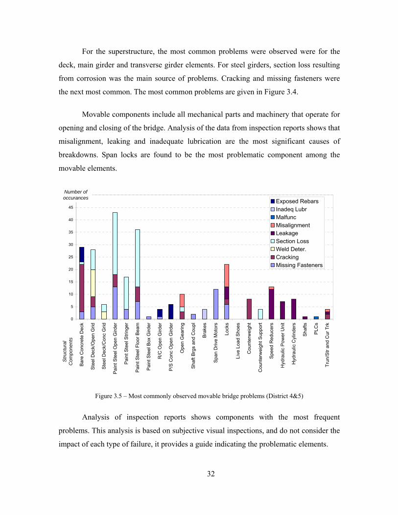
32
For the superstructure, the most common problems were observed were for the
deck, main girder and transverse girder elements. For steel girders, section loss resulting
from corrosion was the main source of problems. Cracking and missing fasteners were
the next most common. The most common problems are given in Figure 3.4.
Movable components include all mechanical parts and machinery that operate for
opening and closing of the bridge. Analysis of the data from inspection reports shows that
misalignment, leaking and inadequate lubrication are the most significant causes of
breakdowns. Span locks are found to be the most problematic component among the
movable elements.
0
5
10
15
20
25
30
35
40
45
50
Bar
e C
oncr
ete
Dec
k
Ste
el D
eck/
Ope
n G
rid
Ste
el D
eck/
Con
c G
rid
Pai
nt S
teel
Ope
n G
irder
Pai
nt S
teel
Stri
nger
Pai
nt S
teel
Flo
or B
eam
Pain
t Ste
el B
ox G
irder
R/C
Ope
n G
irder
P/S
Con
c O
pen
Gird
er
Ope
n G
earin
g
Sha
ft Br
gs a
nd C
oupl
Bra
kes
Spa
n D
rive
Mot
ors
Lock
s
Live
Loa
d S
hoes
Cou
nter
wei
ght
Cou
nter
wei
ght S
uppo
rt
Spee
d R
educ
ers
Hyd
raul
ic P
ower
Uni
t
Hyd
raul
ic C
ylin
ders
Sha
fts
PLC
s
Trun
/Str
and
Cur
Trk
Exposed RebarsInadeq LubrMalfuncMisalignmentLeakageSection LossWeld Deter.CrackingMissing Fasteners
Number ofoccurances
Stru
ctur
alC
ompo
nent
s
Figure 3.5 – Most commonly observed movable bridge problems (District 4&5)
Analysis of inspection reports shows components with the most frequent
problems. This analysis is based on subjective visual inspections, and do not consider the
impact of each type of failure, it provides a guide indicating the problematic elements.

33
3.3.2. Inspection Data Analysis for Christa McAuliffe Bridge over 30 Years
Bascule bridges constitute by far the majority of movable bridge types. Based on
this analysis and interaction with FDOT structures and maintenance engineers, the
bascule type was selected for detailed investigation, and the movable bridge over Florida
SR-3, known as Christa McAuliffe Bridge, was selected as the representative bridge
considering its type, span length, age, opening frequency, type of traffic and accessibility
(Figure 3.6).
The selected representative movable span has the structure number 700072, and is
the south-bound span of two parallel spans on SR-3, crossing the Barge Canal in Merritt
Island, FL. This span was constructed in 1961, and underwent extensive rehabilitation
twice, in 1994-1995 and again in 1999-2003. It has double bascule leaves, each 70-ft
long, and 40-ft wide, carrying two traffic lanes. The representative bridge opens about 6
to 7 times a day.
Figure 3.6 – Case Study: Christa McAuliffe Bascule Bridge in Merritt Island, FL

34
Christa McAuliffe is of the most common bascule type, with a rack-and-pinion
mechanism. The bascule leaves are lifted horizontally at the point of the trunnions, which
are the pivot points on the main girders (Figure 3.7). The weight of the span is balanced
with a counterweight that minimizes the required torque to lift the leaf. The
counterweight is made of cast-in-place concrete. In the closed position, the girder rests on
a support called ‘live load shoe’ on the pier and traffic loads are not transferred to the
mechanical system.
Figure 3.7 – Main girder of Christa McAuliffe Movable Bridge
The movable bridge also involves fixed components, such as reinforced concrete
piers and approach spans. The counterweight of the main girder stays below the approach
span deck in the closed position. When the bridge is opening, the leaves rotate upwards,
and the counterweight goes down. The elevation view of the Christa McAuliffe Bridge is
shown in Figure 3.8.
Figure 3.8 – Christa McAuliffe Movable Bridge elevation (adapted from Christa McAuliffe Bridge
construction plans)

35
The schematic of the mechanical system that operates the movable bridge is
shown in Figure 3.9. The driving torque is generated by an electrical motor, which is then
distributed to the drive shafts via the gear box. The gear box involves an assembly of
gears operating similar to automobile differentials, and provides equal lifting of both
sides. The drive shafts transmit the torque to the final gear called the pinion, which
engages the rack assembly, which is directly attached to the main girder.
Figure 3.9 – Christa McAuliffe Movable Bridge mechanical system (adapted from Christa McAuliffe
Bridge construction plans)
Inspection reports of the representative bridge were analyzed in order to track the
change of condition states over a 25-year period. Examples of the analysis are given in
Figures 3.10 to 3.13, showing the condition state of steel girders and some movable parts
through years. It should be noted that prior to 1980’s movable parts were not assigned
any condition state number, therefore those were not included.
These figures clearly indicate the deterioration pattern and effect of rehabilitation.
The condition of steel girder elements starts deteriorating after 7 or 8 years with the effect
of surface corrosion, section loss and operating impacts causing bents and misalignment.
Each rehabilitation effort, shown as striped regions, produces a positive effect on the
condition state. The downward drift is much more rapid for the case of movable parts,

36
since they are subjected to heavy fatigue effects, and are very sensitive to alignment,
lubrication and proper maintenance.
1
1.5
2
2.5
3
3.5
4
4.5
5
1969
1971
1973
1975
1977
1979
1981
1983
1985
1987
1989
1991
1993
1995
1997
1999
2001
2003
2005
Date
Insp
ectio
n R
atin
g
Concrete Deck
Steel Deck/Open Grid
Steel Deck/Conc Grid
cracking
Rehabilitation
FM 2
37734
WPI
511-0
446
Figure 3.10 – Condition state: Decks
1.0
1.5
2.0
2.5
3.0
3.5
4.0
4.5
5.0
1982
1983
1984
1985
1986
1987
1988
1989
1990
1991
1992
1993
1994
1995
1996
1997
1998
1999
2000
2001
2002
2003
2004
2005
Date
Insp
ectio
n R
atin
g
ShaftsBrgs and CplsEmergency DriveSpan Drive Motor
RehabilitationFM
237734
WPI
511-0
446
corrosion
inadeq. lubrication
Figure 3.11 – Condition state: Movable components
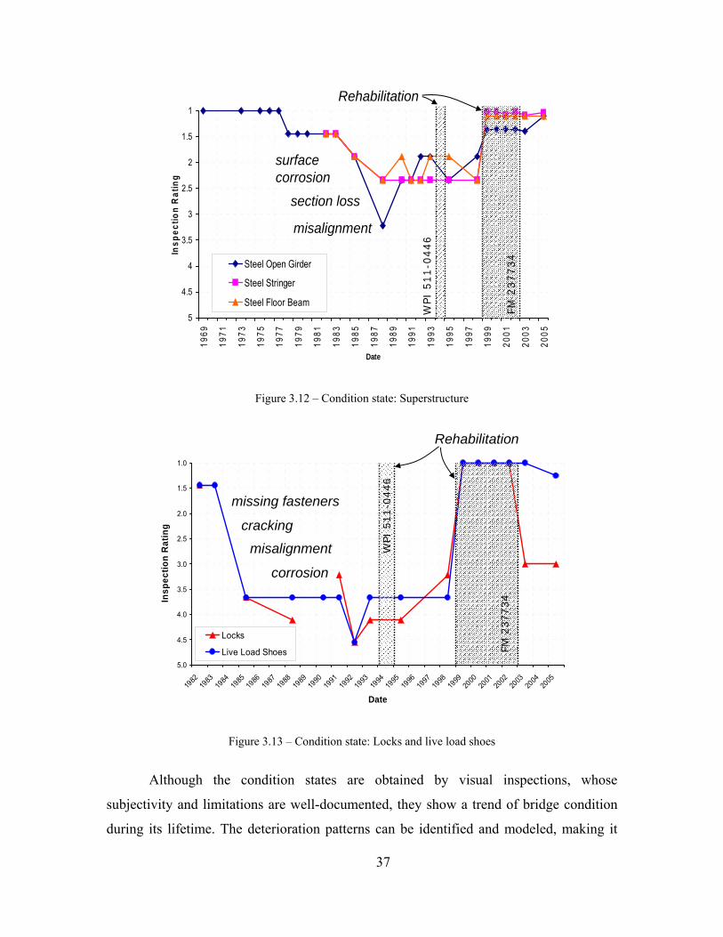
37
1
1.5
2
2.5
3
3.5
4
4.5
5
1969
1971
1973
1975
1977
1979
1981
1983
1985
1987
1989
1991
1993
1995
1997
1999
2001
2003
2005
Date
Insp
ectio
n R
atin
g
Steel Open Girder
Steel Stringer
Steel Floor Beam
Rehabilitation
misalignment
section loss
surfacecorrosion
FM 2
37734
WPI
511-0
446
Figure 3.12 – Condition state: Superstructure
1.0
1.5
2.0
2.5
3.0
3.5
4.0
4.5
5.0
1982
1983
1984
1985
1986
1987
1988
1989
1990
1991
1992
1993
1994
1995
1996
1997
1998
1999
2000
2001
2002
2003
2004
2005
Date
Insp
ectio
n R
atin
g
Locks
Live Load Shoes
Rehabilitation
cracking
misalignment
missing fastenersFM
237734
WPI
511-0
446
corrosion
Figure 3.13 – Condition state: Locks and live load shoes
Although the condition states are obtained by visual inspections, whose
subjectivity and limitations are well-documented, they show a trend of bridge condition
during its lifetime. The deterioration patterns can be identified and modeled, making it

38
possible to predict the future condition and effects of rehabilitation. Here, structural
health monitoring can provide a benefit for reducing the uncertainty in the component
condition appraisal process and supplying dependable data for deterioration analysis.
Accurate structural capacity or a reliability index of each component can be derived with
SHM data, and deterioration models can be constructed by applying the Bayesian
updating method to collected data.
3.4. NUMERICAL MODEL DEVELOPMENT FOR ANALYTICAL EVALUATION OF
STRUCTURAL PERFORMANCE
3.4.1. Finite Element Model Development
Finite Element Modeling is the analysis method based on discretization of
structures to solve the governing equations of mechanics. Computer programs are used to
model the structure. Data from the model are translated into assembled stiffness matrices
to be solved for the input load cases. Finite Element Modeling allows for predicting the
structural response to various loading simulations with much higher accuracy than the
usual simplified analysis techniques.
Development of a Finite Element Model requires attention to the underlying
equations for the elements defined to represent structural components. Appropriate finite
elements should be used to conduct a behavior as similar as possible to the actual
structure. Also, discretizations, connections and constraints of the elements are as
important as matching the geometric requirements. A thorough inspection and
verification stage is crucial to ensure the model has the intended behavior. Two levels of
verification are element-by-element checking and checking the model behavior for
different analysis cases.
3.4.2. Initial Finite Element Model with Shell Elements
An initial model was developed by modeling the main girders with shell elements.
The main girder is a built-up plate girder made out of multiple layers of steel plates. Both
the thickness and the section depth are variable, to provide sufficient capacity at all

39
sections with minimum weight. Flange thickness is also variable, with changing thickness
and number of steel plates through the length of the girder.
Original construction plans were used to build the CAD and Finite Element
models of the bridge. Model creation was also assisted by the notes and pictures obtained
from site visits to the movable bridge (Figure 3.14 and Figure 3.15).
Figure 3.14 – 3D CAD model of the movable bridge

40
Figure 3.15 – 3D CAD model; orthogonal views
The main girder was modeled by using two shell elements for the flanges and one
shell element for the web. Due to the thickness of the elements, their nodes do not match;
therefore, connectivity was satisfied by assigning rigid links as shown in Figure 3.16. The
depth of the girder web varies following a parabolic function, which can be replicated
with shells of varying depth (Figure 3.17).
Figure 3.16 – Modeling of the bascule girder
Rigid Links Shell
Elements

41
Figure 3.17 – Modeling of bascule girders with shell elements
The trunnion was modeled as a circular region connected to the girder shells with
rigid links. This rigid region representing the trunnion-hub-girder (THG) assembly was
assumed to be including the effects of the stiffeners at the trunnion.
Figure 3.18 – Detail of the pinned connection
For all remaining beam members, meaning floor beams, transverse beams and
bracings members, frame elements were employed. In the case of variable linear section
members, also variable frame section elements were used (Figure 3.19).

42
Figure 3.19 – Model with shell elements (deck not shown)
It is important to note that because different frame elements, like W27×102 and
W16×36 have different centers of gravity, a rigid link between them is necessary to
ensure a good model (Figure 3.20).
Figure 3.20 – Rigid links between frame elements
The deck of the movable bridge is steel grid type, built by closely arranged and
welded thin plate members providing maximum bending resistance with minimum self-
weight. Details are given in Figure 3.21, which is from the original construction plans.

43
Figure 3.21 – Detail of the steel deck (Christa McAuliffe Bridge construction plans)
This same type of structure could be modeled in the Finite Element Model using
frame elements (Figure 3.22), but the processing time would be very long and generation
of element would take a long time as well. That is why, a simpler deck was employed,
formed by shell elements equivalent to the real deck of the bridge.
Figure 3.22 – Model of the real deck
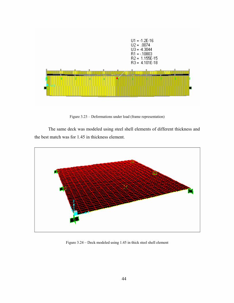
44
Figure 3.23 – Deformations under load (frame representation)
The same deck was modeled using steel shell elements of different thickness and
the best match was for 1.45 in thickness element.
Figure 3.24 – Deck modeled using 1.45 in thick steel shell element

45
Figure 3.25 – Deflections under load (shell representation)
Comparing the results for deflection and rotations it is evident that the modeled
finite element deck behaves similarly to the real one with only a minimum error (Figures
3.23 to 3.25).
The connection between the two spans was modeled using rigid links and the
moments at the contact points were released. Therefore, it was assumed that the shear
force was completely transferred between the two leaves, which is the desired function of
the span lock (Figure 3.26). Since recent changes in design standards require that the span
locks should not be considered as load transferring members, the model was analyzed
with and without the effect of span locks.

46
Figure 3.26 – Connection of two spans
Figure 3.27 – Finite element model with shell elements
This initial model is formed by 230 elements, 29498 shell elements, 2 solid
elements, 4,473 links and 26,808 constrains formed. This model consists of 11,133
master degrees of freedoms and was solved with a system of 178,507 equilibrium
equations and 4,745,459 non-zero stiffness terms. The system was solved using a desktop
computer with Pentium-4, 2.4GHz CPU clock, 1.0 GB memory ram, and the
computational time was 16:14 min as shown in Figure 3.28.

47
Figure 3.28 – Summary of initial finite element model
3.4.3. Modified Finite Element Model with Frame Elements
Since the computational time and complexity of the initial finite element with
shell elements is large, a modified model was developed, replacing the main girders with
variable cross-section frame elements (Figure 3.29).

48
Figure 3.29 – Modeling of bascule girders with frame elements
Transverse girders, floor girders and bracings were also simulated using frame
elements (Figure 3.30). All the members were interconnected using rigid links at their
center of gravity, transmitting moment and other internal forces accordingly.
Figure 3.30 – Main girders, transverse girders, floor beams, and bracings.
Counterweight was simulated using solid concrete elements. The deck was
modeled using 1.45 in. steel shell elements as explained in section 3.4.1. For this model,
the trunnion was defined as a pin connection, instead of a rigid area. The live load shoe

49
(LLS) was again defined as a roller support, since the leaves only rest on the LLS at
closed position (Figure 3.31 and Figure 3.32). Figure 3.33 represents the complete
modified FEM.
Figure 3.31 – Close-up on the trunnion in the modified model
Figure 3.32 – Supports (boundary conditions) of the model (deck not shown)

50
Figure 3.33 – Completed modified FEM (Deck not shown).
This model is formed by 454 frame elements, 3098 shell elements, 4 solid
elements, 450 links and 2706 constrains formed. This model consists of 1480 master
degrees of freedoms and was solved with a system of 18,256 equilibrium equations and
470,034 non-zero stiffness terms. The system was analyzed for static loads using a
desktop computer Pentium 4 CPU 2.4 GHz, 1.00 GB of RAM and the computational time
was 57 sec. as shown in Figure 3.34.
Figure 3.34 – Analysis details for the modified FEM

51
3.5. COMPARISON OF THE TWO MODELS
Both models were compared to be sure they simulate the bridge in the same way.
The validity of the modified model was ensured by obtaining responses for the same
loading and analysis cases. The first structural response to compare the two models was
the tip deflection under static loading. For this purpose, a load corresponding to an HL-93
Truck was placed on both models as show in Figure 3.35.
Figure 3.35 – Load case studied for model comparison
In Figure 3.36 results for deflection on the tip of the leaves are shown for both,
the initial and the modified model.
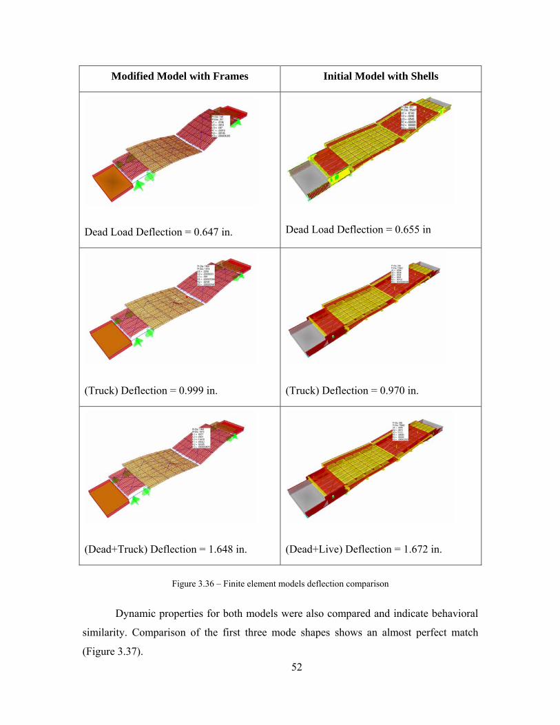
52
Modified Model with Frames Initial Model with Shells
Dead Load Deflection = 0.647 in.
Dead Load Deflection = 0.655 in
(Truck) Deflection = 0.999 in.
(Truck) Deflection = 0.970 in.
(Dead+Truck) Deflection = 1.648 in.
(Dead+Live) Deflection = 1.672 in.
Figure 3.36 – Finite element models deflection comparison
Dynamic properties for both models were also compared and indicate behavioral
similarity. Comparison of the first three mode shapes shows an almost perfect match
(Figure 3.37).

53
Modified Model with Frames Initial Model with Shells
T = 0.271 s f = 3.69 Hz
T = 0.272 s f = 3.68 Hz
T = 0.211 s f = 4.74 Hz
T = 0.196 s f = 5.10 Hz
T = 0.111 s f = 9.04 Hz
T = 0.112 s f = 8.93 Hz
Figure 3.37 – Comparison of the first three principal modes
Based on these comparative results, all further calculations were done using the
modified model, mainly because computational time was reduced by 94% without losing

54
accuracy. The initial model was only used to obtain stress distribution over the girder
when necessary.
3.6. EXPERIMENTAL STUDIES CONDUCTED AT THE BRIDGE
Movable bridge operation is based on the balance of the span weight and the
counterweight. When the weights of the leaf and counterweight are in equilibrium about
the pivot point (trunnion), they are in what is called balanced condition. However, this is
not the desired configuration. Weights of the leaf and counterweight should be distributed
in such a way that the leaf can be closed manually without too much effort in the event of
a power failure. There are no accepted standards for this weight distribution, however,
maintenance engineers agree that this condition should make the leaf drift slowly
downward without power during most of the closing operation. At the same time, the
motor should make the minimum torque to overcome the static friction.
Center of gravityTrunnion Center of gravityTrunnion
Figure 3.38 – Desirable Balance Condition of a Bascule Bridge
The Florida Department of Transportation is using Bascule Bridge Balance Tests
(Malvern et al. 1982) for evaluating the balance state and verify the functioning of the
shaft-gear-trunnion system. A test team of engineers from the FDOT State and Materials
Office in Gainesville conducts these tests by visiting the bridges annually, or whenever
there is a rehabilitation or alteration, which could change its balance condition. The test is
performed by mounting strain sensors on the main drive shafts to obtain the torsional
shear strain. These data are used to calculate the torque during opening and closing of the
leaves, recorded in conjunction with the opening angle, which is obtained by a tiltmeter

55
near the trunnion. Typical plots of average torque (AVT), which is the average of
opening and closing torques, with respect to the opening angle θ, are given in Figure
3.39. The average torque changes with the horizontal distance between the trunnion and
center of gravity, thus, it is a cosine curve. The positive region of this plot is unbalance
towards the leaf side, and the negative region corresponds to unbalance towards the
counter-weight (heel) side.
TrunnionCenter of Gravity
TrunnionCenter of Gravity
TrunnionCenter of Gravity
TrunnionCenter of Gravity
Figure 3.39 – Different cases of average torque during opening and closing
AVT is affected by environmental conditions, such as wind, and the friction in the
system, which acts in the opposite direction of the movement. The friction is obtained
from the difference between the opening and closing torques, as per the equation below;
2co
fTT
T−
= (3.1)
where Tf is the friction torque, To is the opening torque and Tc is the closing
torque. The friction number is indicative of lubrication on the trunnion, rack and gears, as
well as related mechanical problems. Although there are no quantitative limits,
maintenance is required when the friction number is calculated to be relatively high, in
comparison with the previous values.

56
3.6.1. Field Test Data Analysis (Balance Test)
The writers and FDOT personnel conducted bridge balance tests on two different
movable bridges. The bridges were instrumented as described before. The raw data were
provided by FDOT to the writers for analysis. In addition, the writers obtained data from
past studies to track the bridge balance characteristics. Also, it is essential to determine
the correlation between environmental conditions such as wind and the bridge balance,
which may vary depending on when the test is conducted. The writers plan to collect
environmental data in their future tests.
Average torque and friction torque were calculated and plotted against the
rotation angle for Christa McAuliffe Bridge (Figure 3.40). The comparison of the three
tests performed on different dates shows that the balance test results change significantly,
affected by all rehabilitation, alteration and maintenance works, as well as due to possible
deterioration effects. Although reduction of the total imbalance and friction can be
associated with the overall rehabilitation work, the root reasons of the change in
imbalance and friction numbers should be further explored. In the current practice, the
change in friction with respect to baseline is considered and some rules of thumb in terms
of bridge balance are employed based on the engineers’ experience. To track the bridge
balance and imbalance and their interaction with other phenomena such as environmental
effects, it is clear that the balance tests should be part of the movable bridge SHM
application, to be performed real-time for each bridge operation in order to track the
balance condition dependably and identify the interaction of deterioration and
maintenance actions.

57
Figure 3.40 – Balance test results for March 2003
Figure 3.41 – Balance test results for February 2003

58
Figure 3.42 – Balance test results for February 2006
The average torque curves from the three tests at Christa McAuliffe Bridge are
similar, indicating similar balance conditions. However, there does not exist a rationale to
judge if the average torque values are within acceptable values. Standards need to be set,
justifying the limits of average torque values and the friction numbers. As seen in Figure
3.43, friction coefficient changes radically at each test, and it can only intuitively be
related to the change of condition in the system. The majority of the friction is assumed
to be coming from the trunnion friction; therefore, the lubrication in the trunnion is
closely related to the friction numbers. The relation between the friction number and the
trunnion maintenance should be studied, and thresholds should be established for
trunnion lubrication.

59
23.42
13.97
5.91
0
5
10
15
20
25Fr
ictio
n N
umbe
r (K
ips-
ft)
02/11/03 05/06/03 02/21/06
Date
Christa McAuliffe Bridge. Friction Number
Figure 3.43 – Change of friction values

60
4. MODEL CALIBRATION, SIMULATIONS AND RATING
4.1. INTRODUCTION
In this section, the finite element model is calibrated using balance test data, and
several simulations have been conducted to evaluate the response of the structure and
also to determine possible instrumentation locations. As a result, analytical studies
enabled the researchers to understand the structural behavior of the bridge, as well as
determining the roles of the critical components, such as the trunnions, live load shoes,
and the span locks. Analysis results and load rating helps with assessing the current
condition of the bridge and predicting possible structural problems, therefore, enabling an
instrumentation layout plan that can capture the major features identified from the
analyses. All the analyses were conducted after calibrating the finite element model to
match the balance data that was collected by a field test, since the balance condition is
very critical for bascule cases, and the model needs to be calibrated to reflect the actual
behavior.
4.2. CALIBRATION OF THE MODEL ACCORDING TO THE BALANCE CONDITION
The balance condition of the leaves was made to represent the same results with
the latest balance test conducted on the Christa McAuliffe movable bridge. The test was
performed by FDOT Materials Lab personnel and accompanied by UCF researchers. The
FDOT staff supplied the raw data and the test results, which were then analyzed by the
UCF researchers. The analysis procedure and results are given in Section 3.3.1, and they
were also used to calibrate the finite element model of the bridge. In order to provide the
same balance condition, only a single leaf of the bridge model was analyzed, fixing at the
trunnion and removing the live load shoe support. The weight of the counterweight was
adjusted by iteration to match with the calculated imbalance moment.

61
Figure 4.1 – Balance condition of the leaves
4.3. ANALYSIS AND LOAD SIMULATION RESULTS
4.3.1. Loads Used for FE Simulations
The bridge model was analyzed under a vehicular load corresponding to the
AASHTO HL-93 design truck.
Figure 4.2 – AASHTO HL-93 Design Truck

62
Figure 4.3 – Loading for load rating and serviceability of the bridge
(Two HL-93 trucks and distributed lane load)
Once finished and loaded, the model realized the analysis of the bridge showing
the following results.
4.3.2. Deflections
Deflection was calculated from the finite element model analysis with two HL-93
standard truck loading and lane loading as specified by the AASHTO Manual. Load
factors are 1.0 since deflection is a serviceability check. The allowable deflection
specified is δmax = L/300 for orthotropic plate decks with vehicular load on deck
(AASHTO 2.2.2.6.2), where L is the span length, 140 ft in the current case. The
deflection was checked to be below this specified value. Figure 4.4 shows the deflected
shape and the displacement values at the tips.
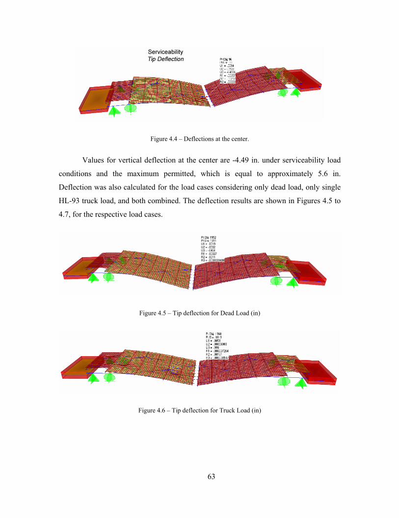
63
Figure 4.4 – Deflections at the center.
Values for vertical deflection at the center are -4.49 in. under serviceability load
conditions and the maximum permitted, which is equal to approximately 5.6 in.
Deflection was also calculated for the load cases considering only dead load, only single
HL-93 truck load, and both combined. The deflection results are shown in Figures 4.5 to
4.7, for the respective load cases.
Figure 4.5 – Tip deflection for Dead Load (in)
Figure 4.6 – Tip deflection for Truck Load (in)

64
Figure 4.7 – Tip deflection for Dead Load and Truck Load (in)
4.3.3. Stresses
Von Mises stress, based on the yield criterion of the same name, is defined as;
( ) ( ) ( )[ ]222
231
221vm 2
1 σ−σ+σ−σ+σ−σ=σ (4.1)
where σ 1, σ 2 and σ 3 are the principal stress values at the point of concern. For
steel plate structures, Von Mises stress is a better indication of the yielding condition,
since the stresses are usually biaxial. The initial model with shell elements was evaluated
to obtain the Von Mises stress distribution over the main girders. The initial model with
shell elements was evaluated to obtain the Von Mises stress distribution over the main
girders, and the results for only dead load, only truck load and combination are shown in
Figures 4.5, 4.6 and 4.7, respectively. In this analysis, load factors have not been used.
Von Mises stresses due to combined dead and live load are seen to be around 6-12 ksi
(Figure 4.7) compared to 36 ksi yield stress of the steel girders.
Figure 4.8 – Von Mises stresses for Dead Load (ksi)

65
Figure 4.9 – Von Mises stresses for Truck Load (ksi)
Figure 4.10 – Von Mises stresses for Dead Load and Truck Load (ksi)
Figure 4.11 – Von Mises stresses at the THG connection for Dead Load (ksi)

66
Figure 4.12 – Von Mises stresses at the THG connection for Truck Load (ksi)
Figure 4.13 – Von Mises stresses at the THG connection for Dead Load and Truck Load (ksi)
Figures 4.8, 4.9 and 4.10 show the Von Mises stress distributions around the
trunnion region for only dead load, only truck load and combined, respectively. One of
the highest stress levels (around 12 Ksi) is observed at the trunnion region, since it is
where the total moment is resisted (Figure 4.10). As an extreme condition, the live load

67
shoe was removed for this analysis in order to simulate the opening action, when all the
balance is provided by the driving torque at the trunnion.
Another high stress concentration occurs at the span lock (Figure 4.7). Here,
stress values of around 10 ksi were observed. It is important to notice that this is an area
subjected to constant impact from the traffic and is highly susceptible to fatigue.
The live load shoes and the girder area in contact with them is another high-stress
location also prone to fatigue. Stress values are around 15 ksi for these particular
positions when bridge is in closed position and loaded as shown in Figure 4.3. We also
note that high stress values are localized and numerical model results for stresses are to
be verified with field measurements.
4.3.4. Dynamic Analysis
Dynamic analysis of the finite element model provided the natural modes and
frequencies of the structure. Mode shapes also provide another means of checking the
model for accuracy and errors as well as global response of the bridge (Figures 4.11 to
4.16).
Figure 4.14 – Modal analysis results: Mode 1

68
Figure 4.15 – Modal analysis results: Mode 2
Figure 4.16 – Modal analysis results: Mode 3
Figure 4.17 – Modal analysis results: Mode 4
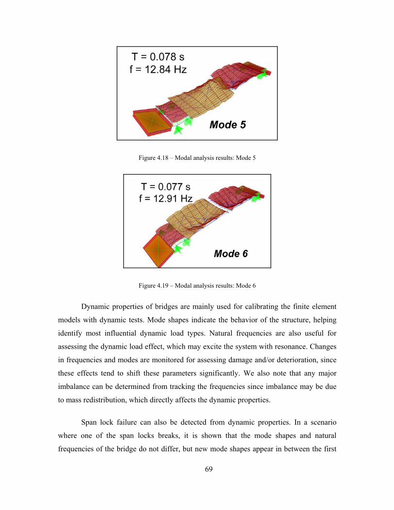
69
Figure 4.18 – Modal analysis results: Mode 5
Figure 4.19 – Modal analysis results: Mode 6
Dynamic properties of bridges are mainly used for calibrating the finite element
models with dynamic tests. Mode shapes indicate the behavior of the structure, helping
identify most influential dynamic load types. Natural frequencies are also useful for
assessing the dynamic load effect, which may excite the system with resonance. Changes
in frequencies and modes are monitored for assessing damage and/or deterioration, since
these effects tend to shift these parameters significantly. We also note that any major
imbalance can be determined from tracking the frequencies since imbalance may be due
to mass redistribution, which directly affects the dynamic properties.
Span lock failure can also be detected from dynamic properties. In a scenario
where one of the span locks breaks, it is shown that the mode shapes and natural
frequencies of the bridge do not differ, but new mode shapes appear in between the first

70
three modes. These new modes can easily be identified from vibration tests, determining
instantly any failure of the span locks.
Figure 4.20 – Additional mode shapes for a span-lock failure scenario
4.3.5. Examples of Location for Monitoring Based on FEM
Trunnion is the pivot point of rotation for the bascule leaf. According to FHWA,
fracture critical member is “a member in tension, or with a tension element, whose failure
would probably cause a portion of or the entire bridge to collapse.” (FHWA Report
2002). Therefore, trunnions can be accepted as fracture critical components for the
operation of the movable bridges. The FE model also indicates high stress concentration
in the vicinity of the trunnion.
Connection between the girder and the trunnion is a highly critical location, where
problems such as cracking, misalignment and corrosion are commonly observed. It is a
very important part of the mechanical system, and it should be monitored.

71
Figure 4.21 – Span lock failure simulation
Span lock, which holds the two spans together and assures the same vertical
displacement of the tips is also critical. The effect of failure of the span lock was
investigated by removing the links connecting both leaves at the tips in the finite element
model. When the span lock is removed, the model shows that the leaves deform
independently of each other causing up to approximately 1.5 in. difference in vertical
displacement. Monitoring and maintenance of the span locks is essential to ensure proper
function.
4.4. MOVABLE BRIDGE LOAD RATING
Load rating analysis is another approach to evaluating live load carrying capacity
of the bridges. Load rating also indicates the critical locations and often load rating
results of FEM can further be verified by experimental measurements.
Load rating of the movable bridge was calculated following the AASHTO Guide
(AASHTO 2002). Bending capacity, including lateral torsional buckling effect, and shear

72
capacity were calculated as deterministic values. Critical positions of the standard
(HL-93) truck load were used to obtain the maximum live load moment and shear. The
sections selected for load rating are the joints at the floor beams.
Figure 4.22 – Transverse loading
Figure 4.23 – Truck position for load rating (lane load not shown)
The transverse cross-section of the deck (Figure 4.22) shows the location of the
lanes and axle positions for the HL-93 standard truck loading. Since a three-dimensional
model was used, axle loads were defined as individual point loads, and lane loading was
ignored. The truck was placed at the midspan of the movable bridge, for the most critical
loading condition, as shown in Figure 4.23.

73
The load rating can be expressed as the factor of the critical live load effect to the
available capacity for a certain limit state. The general formula for the rating factor is;
( )IM1LLPDWDCC
RFL
pDWDC
+γ
γ±γ−γ−= (4.2)
where C is the factored load carrying capacity, DC is the dead load of structural
components, DW is the dead load of the wearing surface, P is a dead load
concentrated at a single point, LL is the live load effect, IM is the impact factor,
and γ’s are the safety factors.
Figure 4.24 – Section locations for load rating
The load factors change according to the type of load rating, i.e., inventory load
rating or operating load rating. The load ratings for the girder were calculated at the
connections of the floor beams, as indicated in Figure 4.24. The capacity of the sections
were calculated based on the ultimate moment capacity
ZFM yu = (4.3)
where Mu = ultimate moment capacity; Fy = specified yield strength;
Z = plastic section modulus.
The yield strength of the steel was given as 36.0 ksi. The plastic moduli was
calculated from section sizes in the CAD drawing. Area of the bolts was deducted from
the section size while calculating the plastic modulus. Then, following formula (1), the
section moment capacities were found for the three sections as:

74
Table 4.1 – Section flexural capacity
Location Z (in3) Mu (kip·ft) Mu (kip·in)
FB-1 137.5 4951.9 59422.8
FB-2 73.2 2634.8 31617.6
FB-3 29.4 1057.5 12690.0
The load effects (moments) on the sections were obtained from finite element
analysis with the loading pattern shown in Figure 4.22.
Table 4.2 – Section moments from the load combination
Location MDL (kip·in) MLL-TRUCK (kip·in) MLL-LANE (kip·in)
FB-1 8805.0 16579.5 4676.8
FB-2 3644.0 4321.3 1289.2
FB-3 940.4 1659.5 300.4
The dynamic impact factor is used as 33% for both inventory and operating
ratings. The load factors change according to the rating type as follows;
Table 4.3 - Load factors
Load Rating Case Load Factor (γ) Inventory Operating
DC 1.25 1.25
DW 1.25 1.25
LL+IM 1.75 1.35
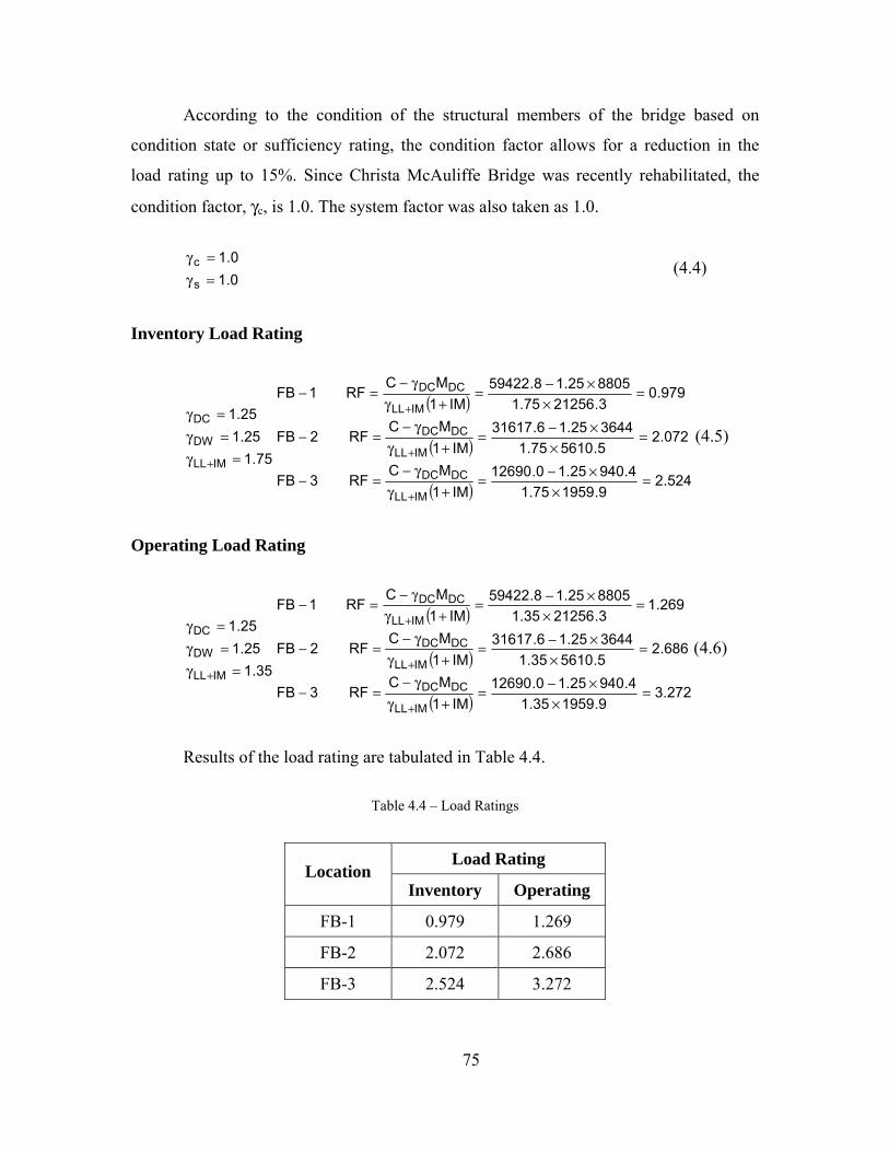
75
According to the condition of the structural members of the bridge based on
condition state or sufficiency rating, the condition factor allows for a reduction in the
load rating up to 15%. Since Christa McAuliffe Bridge was recently rehabilitated, the
condition factor, γc, is 1.0. The system factor was also taken as 1.0.
0.10.1
s
c=γ=γ (4.4)
Inventory Load Rating
75.125.125.1
IMLL
DW
DC
=γ=γ
=γ
+
( )
( )
( ) 524.29.195975.1
4.94025.10.12690IM1
MCRF3FB
072.25.561075.1364425.16.31617
IM1MC
RF2FB
979.03.2125675.1880525.18.59422
IM1MC
RF1FB
IMLL
DCDC
IMLL
DCDC
IMLL
DCDC
=×
×−=+γ
γ−=−
=×
×−=+γ
γ−=−
=×
×−=+γ
γ−=−
+
+
+
(4.5)
Operating Load Rating
35.125.125.1
IMLL
DW
DC
=γ=γ
=γ
+
( )
( )
( ) 272.39.195935.1
4.94025.10.12690IM1
MCRF3FB
686.25.561035.1364425.16.31617
IM1MC
RF2FB
269.13.2125635.1880525.18.59422
IM1MC
RF1FB
IMLL
DCDC
IMLL
DCDC
IMLL
DCDC
=×
×−=+γ
γ−=−
=×
×−=+γ
γ−=−
=×
×−=+γ
γ−=−
+
+
+
(4.6)
Results of the load rating are tabulated in Table 4.4.
Table 4.4 – Load Ratings
Load Rating Location Inventory Operating
FB-1 0.979 1.269
FB-2 2.072 2.686
FB-3 2.524 3.272

76
4.5. MOVING LOAD SIMULATION
In order to determine the structural load carrying capacity, moving load
simulations were carried out to obtain the reliability of the bridge in addition to the load
rating. The reliability analysis incorporates a probabilistic approach with respect to the
load effects and structural capacity.
The finite element model was used to simulate a standard AASHTO HL-93 truck
traveling over the bridge. The truck load was applied as joint loads, with 12.5-in
increments, which corresponds to about 0.015s steps for a truck traveling at 50 mph
(Figure 4.25). This simulation was expected to provide the structural reliability of the
bridge, and also simulate the sensor readings during a moving load for using in data-
based reliability assessment.
Figure 4.25 – Moving Load Analysis
The variation of moment values at each node on the main girder on the north span
is shown in Figure 4.26. The horizontal axes in these graphs are the truck position, which
is moving at a constant velocity.

77
Figure 4.26 – Variation of Moment due to Moving Load over the Girder Locations
Statistical Models of Random Variables
Probabilistic modeling of the structural capacity and load effects requires
determination of the statistical parameters with the uncertainties of each parameter.
Sources of variability are generally categorized as material factor (material properties),
fabrication factor (imperfections) and analysis factor (assumptions, approximations)
(Nowak and Collins 2000), and have been quantified by statistical studies in the
literature. At least the mean value and the variance (or standard deviation, or coefficient
of variation) should be known for reliability analysis. In this study, statistical
distributions were used for the random variables.

78
Nodal results obtained from the analytical simulation were taken as the nominal
values of load effects, and assumed as normally distributed. The bias factor (λ) for the
load effect was taken as 1.15, and the coefficient of variation (cov) as 0.18 (Nowak
1995). Bias factor and coefficient of variation of other random variables are used as in
Table 4.5. Yield strength of the structural steel was specified as 36 ksi.
Table 4.5 – Statistical Parameters of the Random Variables
Variable Moment of
Inertia IX
Plastic Section
Modulus Zx
Yield Strength
Fy
Truck Load Mu, Vu
μ (mean) 1.0 1.0 1.12 1.15
δ (c.o.v.) 0.05 0.05 0.0866 0.18
Type Lognormal Lognormal Lognormal Normal
Section properties were obtained for all the locations of concern over the main
girders, and the cross beams. The modulus of inertia and the plastic modulus were taken
as random variables, and used to calculate the yield and plastic moment capacity. The
sections and corresponding properties are shown in Figure 4.27 to 4.26.

79
Figure 4.27 – Section properties of Section 1 along the girder
Figure 4.28 – Section properties of Section 2 along the girder

80
Figure 4.29 – Section properties of Section 3 along the girder
Component Reliability
Component reliability indices were calculated based on moment and shear failure
modes. The main girders constitute the main load carrying components; therefore, they
are the most critical members. Moment and shear failure modes at the sections selected
for instrumentation were evaluated. Cross-beams were also considered for moment
capacity.
For the moment limit state, two cases were considered; yield moment, and the
plastic moment. The limit state function according to the yield moment capacity is;
( ) uxyuxyyieldM MSFM,S,Fg −= (4.7)
where the random variables are Fy (yield strength), Sx (section modulus) and Mu
(applied moment on the section). For the plastic limit case, instead of Sx, plastic section
modulus (Zx) was used, and the limit state function for this case;
( ) uxyuxyplasticM MZFM,Z,Fg −= (4.8)

81
For the shear failure limit state, two random variables were defined. Vr is the
shear capacity, and it was taken as;
ywr FA31V =
(4.9)
where Aw is the web area and Fy is the yield strength of the steel. The shear
capacity was modeled as lognormally distributed. The bias factor λv was taken as 1.14
and the coefficient of variation, 0.106 (Nowak and Collins 2000). The shear load effect
was again taken from finite element model results. The limit state for shear mode is;
( ) ururV VVV,Vg −= (4.10)
The defined limit state functions were evaluated at each joint to obtain the
probability of failure. For nonlinear limit state functions, as in the current case,
convenient first order approximations can be applied using Taylor series expansion to
linearize the function with respect to the random variables. The limit state function is
expanded with respect to each random variable about a certain point on the limit state
surface. The linear approximation will be more accurate in the proximity of this pivot
point, which is also called the design point. The coordinates of the design point are to be
determined, which can be represented as values of the random variables ( ),...x,x,x *3
*2
*1 , or
within the reduced variate space, as ( ),...z,z,z *3
*2
*1 . The distance from the origin to the
design point in reduced variate coordinates gives the reliability index. The limit state
function for plastic moment capacity was expanded around the design point as follows.
( ) ( ) ( )( )
∑= ∂
∂−+≈n
1i x,...,x,xi
*ii
*n
*2
*1n21
*n
*2
*1
XgxXx,...x,xgX,...,X,Xg (4.11)
where X1 : Fy, the yield strength of the steel
X2 : Zx, plastic modulus of the section
X3 : Mu, moment effect on the section due to dead load and moving load

82
The design point is calculated to be the minimum distance from the origin to the
limit state surface in reduced variate space. Therefore, iteration is required for finding the
design point. According to the procedure of the Rackwitz-Fiessler method (Rackwitz and
Fiessler 1978), equivalent normal statistical parameters of the non-normal random
variables were calculated. Since the yield strength (Fy), plastic section modulus (Zx) and
elastic section modulus (Sx) were assumed as lognormally distributed, equivalent normal
mean value and standard deviation of each of these random variables using the following
formulae;
( )[ ]Xln**e
x
Xln*e
x
xln1x
x
μ+−=μ
σ=σ (4.12)
Then, partial derivatives of the limit state function with respect to each random
variable were obtained, and the sensitivity matrix was formed with these values. The
derivatives for the plastic moment limit state were given below as an example. Partial
derivatives for the other limit state functions were obtained similarly.
iXintpodesignii
i
intpodesigniintpodesignii X
gZX
Xg
ZgG σ
∂∂
−=∂∂
∂∂
−=∂∂
−= (4.13)
3
2
i
X3
X12
X21
G
XG
XG
σ=
σ−=
σ−=
{ }⎪⎭
⎪⎬
⎫
⎪⎩
⎪⎨
⎧=
3
2
1
GGG
G (4.14)
An initial design point was assumed for the first cycle of iterations, in order to
obtain the first estimate of the reliability index. The iterative process was set up in
MATLAB software, which used finite element output at the required nodes and
computed the reliability index for all limit state functions and the system reliability for
each given truck position.

83
System Reliability
System reliability is a major concept in reliability analysis, because individual
limit state functions are assembled together in a system model. The failure conditions are
determined by the system model, since failure of one or two members may not be
important due to redundancy. On the other hand, there may be critical components
(fracture-critical) which have to stay intact for the structural integrity of the whole
system.
System reliability can be modeled with certain assumptions, including assembling
the failure limit states as parallel or series links after determining the failure modes.
Evaluation of a system model is performed by reducing first the parallel components.
System failure probability of parallel systems are solved by;
( ) ( )∏=
=n
1kkfif PP , n: # of parallel members (4.15)
Therefore, the model is reduced to only serially connected members. Failure of
each component means failure, so all the components should survive for structural
integrity. So, the resulting series system can be solved by the following;
( ) ( )[ ]∏=
−−=m
1iifsystemf P11P , m: # of series components (4.16)
Parallel and series models of the movable bridge structural components were
constructed according to the most general structural failure mechanisms. The main
components of the system were the main girder bending failure state, main girder shear
failure state, and the moment failure of the transverse beams. The main girder failure
states were assumed as the failure condition at any of the monitored sections. These
sections, however, are not fully independent, therefore cannot be modeled as acting in
series. Accounting for the correlation of the failure probabilities at these sections, two
limit cases were considered. The first case is assuming no correlation between the failure
of monitored sections, which can be modeled as a series system in this case, and the

84
second case is modeling them as fully correlated limit states, so the failure of the main
girder system depends on the section with the highest probability of failure. The system
model is shown in Figure 4.30, which illustrates the lower bounding case.
Figure 4.30 – Movable Bridge System Reliability Model with Parallel/Series Assembly (Lower Bound)
The system reliability was first calculated according to the same load case as
employed for the load rating calculations. Results of the finite element analysis were used
to generate the input variables, and the reliability was obtained as 3.24 for the lower
bound, and 3.37 for the upper bound case and these values can be considered acceptable
since AASHTO LRFD designs are based on a reliability index of 3.5 for new bridges and
AASHTO Load and Resistance Factor Rating (LRFR) considers 2.5 for existing bridges.
Reliability analysis was also performed for the moving load case, where a single
standard truck is simulated crossing the bridge. The results for each position of the truck
were obtained from the finite element simulation and processed by the component and
system reliability algorithms developed in MATLAB. The result of the system reliability
analysis is plotted in Figure 4.31, for plastic moment capacity. The horizontal axis is the
truck position, which can also be regarded as time. The vertical axis shows the reliability
index, which changes according to the position of the truck.
It should be noted that high reliability values obtained from this analysis are due
to the presence of a single truck without lane loading, and also excluding any wind load.
This analysis was conducted to demonstrate the monitoring of reliability at a single

85
instant based on the collected measurements. The minimum reliability index was
calculated as 5.79 when the middle axle of the truck arrives at the midspan. The
calculated reliability is relatively high, since the simulation uses a single truck crossing
the bridge without lane loads or additional load cases.
Figure 4.31 – Instantaneous System Reliability under a Single Moving Truck (note that this is for one
moving truck without lane load, wind, temperature)
The reliability obtained here is not a formal reliability analysis result, since an
instant in time is selected instead of the life span of the structure. This is to demonstrate
the changes in reliability in real time and to layout a framework to incorporate
instantaneous reliability into life-cycle reliability analysis of the structure.
Safety indices based on component or system reliability can be evaluated with
much higher accuracy and confidence over the long term throughout the monitoring
process. Component-based monitoring data should be assessed to produce reliability of
each monitored structural component, and deterioration with time. Components to be
instrumented and the parameters to be monitored should be carefully selected.

86
SHM techniques make it possible to retrieve information about the status of
individual elements of a bridge. Since every component requires unique maintenance
work, these operations can be scheduled more specifically and efficiently. Also, once
individual deterioration and maintenance models are available for each critical node, a
network reliability analysis can be conducted within the bridge components, in order to
determine the most critical components (parallel/series reliability). Structural condition
state and reliability are to be determined from component data. Reliability of the
structural system depends on reliability of its components, so if there is no redundancy,
the weakest link will determine the overall reliability. Presence of redundant members
makes it necessary to perform a system reliability analysis, modeling the structure as
parallel and/or series combinations of the components (Susoy et al. 2006a; Susoy et al.
2006b).
4.6. SUMMARY OF ANALYSIS RESULTS
The results of the finite element model analysis for specific locations are shown in
the table below. The results are listed according to three cases;
Only dead load,
Only a single standard (HL-93) truck at the tip without dead load
Dead load and a standard truck (HL-93) at the tip
Figure 4.32 – Loading position for FEM analysis results

87
Vertical reactions at support locations, which are the trunnion (pin support) and
live load shoe (roller support) are provided. The span-lock shear is also given as it
indicates the load transfer provided by the span-lock assembly. The maximum moment
on the main girders and the transverse beams are shown. Finally, the tip deflections for
the mentioned load cases are included.
Table 4.6 – Summary of analysis results (reactions and deflections)
Feature Units Dead Load Truck Load*
Dead Load + Truck Load*
Reactions
1 Trunnion (kips) 161.74 126.28 288.02
2 LL Shoe (kips) 73.63 138.48 212.11
Shear
1 VSpan-Lock (kips) 7.337 12.92 20.269
Moment
1 max Mgirder (kip·in) 8026.3 11223.8 19250.1
2 max Mtransverse (kip·in) 383.5 1112.5 1495.6
Deflection
1 δtip (in) 0.647 0.999 1.648
* Single HL-93 Truck without lane load applied
** Results are from FEM 2
Stress distributions over the girder and around critical regions are given in the
previous sections. Results of stress distributions indicate the critical regions and aid
understanding of the load transfer mechanism. Stress values around critical features such
as trunnion, live load shoe and span locks are given in Table 4.7. Maximum observed
stresses around the points of interest are reported, although stress values are susceptible
to stress concentrations, meaning shown results can be accepted as conservative.

88
Table 4.7 – Summary of analysis results (stresses)
Location Units Dead Load Truck Load*
Dead Load + Truck Load*
Trunnion (ksi) ~5.1 ~7.5 ~12.6
Live load shoe (ksi) ~6.4 ~8.7 ~15.1
Span lock (ksi) ~5.2 ~6.9 ~12.1
First modal frequencies and periods according to the dynamic analysis of the
bridge are given in Table 4.8.
Table 4.8 – Modal frequencies and periods for the movable bridge
Mode # Mode Type Frequency (Hz) Period (s)
1 Vertical 3.69 0.271
2 Torsional 4.74 0.211
3 Vertical 9.04 0.111
4 Vertical 11.54 0.087
Load rating of the main girder based on HL-93 load case (two trucks each 72 kips
and a lane load of 0.64 kip/ft as shown in Figure 4.22) was calculated, and shown in
Table 4.7 for the position over the live load shoe location. A load rating value below 1.0
means inadequate in terms of strength, therefore, the calculated inventory load rating is
found to be slightly under 1.00. The load rating can be further investigated using actual
SHM data, and rating formulation can be modified using results such as measured
dynamic impact factors.

89
Table 4.9 – Load rating results for the main girder at the LLS
FB-1 FB-2 FB-3
Inventory 0.979 2.072 2.254
Operating 1.269 2.686 3.272
The system reliability of the movable bridge was obtained as 3.24 for the lower
bound, and 3.37 for the upper bound case, for the same load case with the load rating
calculations.

90
5. INTEGRATED STRUCTURAL HEALTH MONITORING
DESIGN
5.1. INTRODUCTION
Data from an SHM system can provide information related to structural
performance as well as condition based maintenance during the monitoring period. For
movable bridges, maintenance of mechanical and electrical components are as important
as maintenance of structural components. The most common types of machinery and
related problems need to be investigated in order to propose monitoring solutions to
detect those problems, track their development, and plan for corrective action before
failure. In this chapter, sensors and data acquisition systems along with data analysis and
management techniques are discussed. At the end of the chapter, critical electrical,
mechanical and structural components for movable bridges are summarized and possible
SHM designs are presented.
5.2. SENSORS AND SENSOR NETWORKS
All kinds of sensors work by transforming physical changes in the environment or
the structure into a measurable signal. Sensors are desired to be insensitive to the changes
in parameters other than the measured quantities. Those physical and/or environmental
changes alter the response of the sensing unit to a given excitation. The relation between
the ratio of response to the input excitation and the measurand is established through
calibration, which is usually provided by the manufacturer and may be repeated at certain
intervals.
The most basic and commonly applied types of measurement parameters are
related with basic physical responses of structures, such as strain, displacement,
acceleration, tilt and environmental conditions such as temperature, wind speed and
direction, and humidity. There are various types of sensors with different technologies,
but here, only the most widely used types and their operation principles will be described
first.

91
In this respect, all sensors have characteristics that specify their measurement
behavior, making them suitable for certain types of applications and unsuitable for others.
The main characteristics of sensors we are concerned with are listed below. The basic
sensor and measurement properties should be specified for all sensors by the
manufacturer, and the other characteristics can be quantified with further calibration tests
(Aktan et al. 2003; Dunn 2005).
Sensitivity: This is the amount of change in the output of a sensor in response to a change
in a sensor’s input. Sensitivity is defined as the ratio of output to input, and is an
important characteristic related with the precision and accuracy of the measurement. It
may be considered as the slope of the calibration line for the sensor measurement.
Resolution: The smallest measurable change in input that will produce a small but
noticeable change in the sensor output. This defines how small a change in the measurand
can be detected by the sensor.
Discrimination: Also referred to as the limit of detection, this is the smallest increment of
a measurement that can be discerned.
Range: The maximum and minimum values of the measured occurrence that can be
measured with the sensor define the range property. Sensors will not be able to capture
the changes beyond those limits.
Hysteresis: The maximum deviation between the measurement obtained by increasing
and decreasing values of the measurement. Hysteresis error can be caused by the sensor’s
physical changes to the reversal of the conditions, or the structure’s inherent hysteresis
behavior. It is specified as the maximum difference between the measurements taken at
both situations.
Accuracy: This is the closeness of a measurement to the value defined to be the true value
of the measurand. The true value refers to an accepted and traceable standard and is
usually compared to the sensor measurement during calibration. Accuracy is a qualitative
concept and is the combined error of nonlinearity, repeatability, and hysteresis. Accuracy

92
is usually expressed as a maximum positive or negative percent of the full scale (FS) of
the output.
Linearity: The measurements usually do not follow the calibration curve over the entire
range linearly. Linearity defines the deviation of measurements from the linear
calibration line.
Repeatability: Obtaining the same output value for repeated measurements of the same
quantity specifies the repeatability of the instrument.
Stability: This refers to the ability of a sensor to maintain its calibration value over an
extended time period. Sensors with good stability are preferred for long-term
measurements in order to avoid the errors due to the drift in the measurements. Drift is
the continuous upward or downward change of measurements mostly due to
environmental effects.
The measurements are subject to errors due to instrumental properties and
uncertainties listed above, as well as other sources. Installation is a major source of
uncertainty, since the measurement location is the point the gage is installed. Installation
quality will vary widely according to the care, skill and expertise of the operator.
Imprecise location, direction and alignment may cause significant errors in
measurements, where improper mounting may even prevent any useful measurements at
all.
Noise, considered as a random oscillation in the signal, is also inherent in all
sensor measurements. The sources could be internal, such as the resistive properties and
effects during signal transfer to the data acquisition device, or external from mechanical
and electromagnetic fluctuations. Measurement noise can be high enough to reduce the
accuracy of measurements significantly, but usually noise components can be eliminated
by filtering. Filtering is the process of screening the input signal according to the desired
ranges of frequency or other parameters. Filtering is explained in the following sections,
as part of the data acquisition system.

93
The sensory system refers to the sensors and their corresponding interfacing units
for input signals gathered from various monitoring equipments. In the design/selection of
the types and locations of sensory systems, the following criteria should be fulfilled
(Wong 2005).
The sensory system should have the ability to capture the local and system-level
responses, which could be correlated or compared with those design values;
The sensory system is required to integrate the predictive-modeling and data
interrogation processes with the sensing system design process;
The sensory system should have the function to acquire data in a consistent and
retrievable manner for long-term statistical data processing and analysis;
All sensors should be chosen from the contemporary commercially available sensors
that best match the defined sensing performance requirements;
The sensory system should include additional measurements by removable/portable
sensors to quantify changing operational and environmental conditions;
At key locations, different types of sensors should be deployed so that cross-
calibration of sensors could be carried out.
5.2.1. Traditional Sensors
The most common types of sensors used in SHM applications include
displacement sensors, strain sensors, vibrating wire sensors (both temperature and
strain/rotation/displacement, etc.), force sensors, and temperature sensors. Displacement
transducers and settlement devices can be used to measure and monitor deflection,
settlement, joint openings, and other movements of bridge members. Strain sensors are
normally used to measure the change in the length of an object per unit length. These
conventional gages are commercially available from various suppliers with different
specifications. Some of the basic characteristics and principles for these gages are given
in the following;
Strain Gages: Probably the most commonly sought monitoring parameter is the
strain, which is the ratio of the change of length of an element to its original length.

94
Strain is directly related with the stress experienced at that location, and provides direct
indication of the utilized and reserve capacity of the location, section or component. For
strain measurements, a reference point is not required, which is a major advantage. There
are many techniques available that can be used to measure strains. The most common
types used for bridge testing and monitoring applications are electrical resistance strain
gages and vibrating wire strain gages.
Electrical resistance gages are usually bonded foil type, consisting of a thin foil of
resistor embedded within a nonconductive plastic film. The difference in strain
measurement is obtained through the change of resistance of the foil as it is stretched or
compressed, together with the structural location. The resistive change is measured
through circuits called ‘bridges’ to increase the accuracy of measurements by measuring
the voltage difference between the legs of the bridge in accordance with the applied
voltage on the bridge.
Figure 5.1 – Example foil type strain gages (Omega Eng.)
Foil strain gages measure strain in a single direction, but for measuring
components of strain in multiple directions, strain gage rosettes made of two or more
strain gages are also available (Figure 5.1). There are many types of resistive strain
gages, which can be installed by mounting on the surface with adhesives, epoxy or
welding, or by embedding inside concrete or similar material.
Vibrating wire strain gages are very reliable and robust gages that operate on the
principle of natural frequency, as shown in Figure 5.2. The vibrating wire is the metal rod
that is fixed on or embedded into the structure, which undergoes deformation. Tension on
the wire due to extension or contraction will change its natural frequency, which is
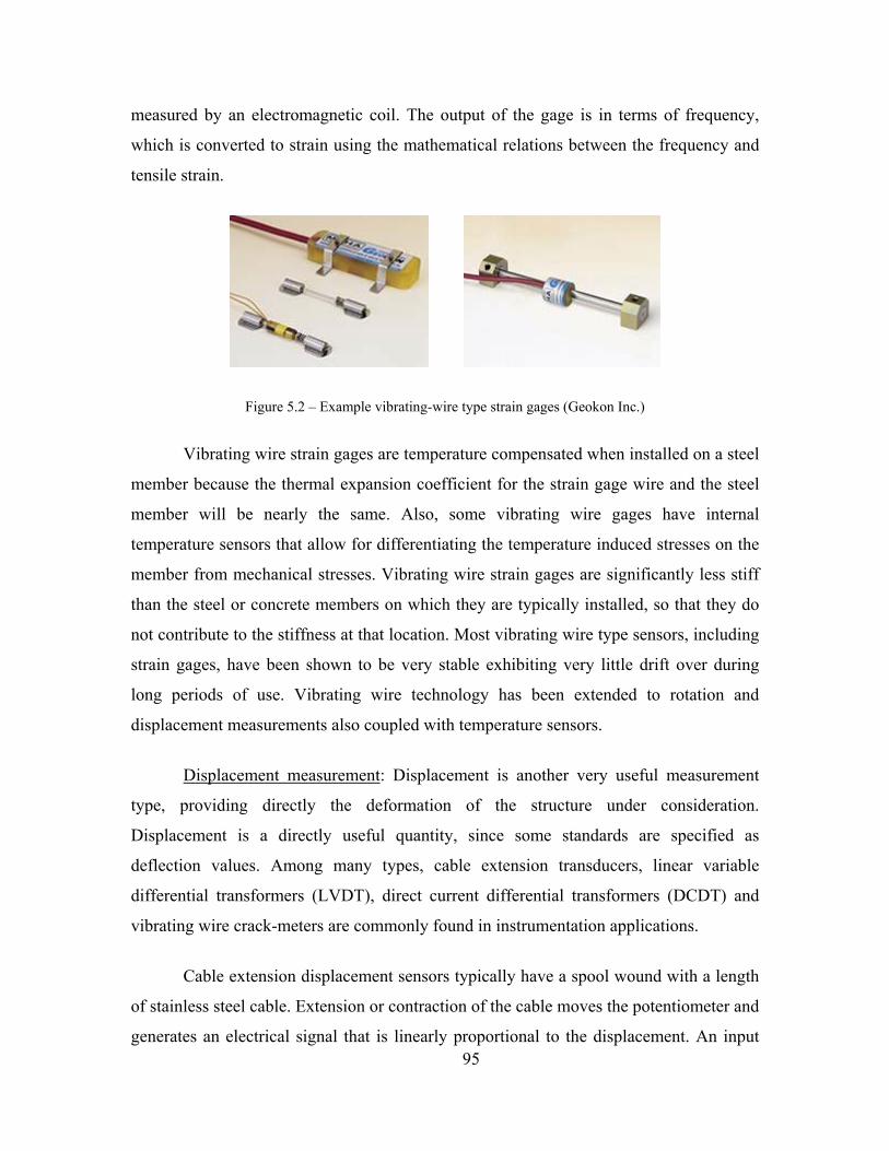
95
measured by an electromagnetic coil. The output of the gage is in terms of frequency,
which is converted to strain using the mathematical relations between the frequency and
tensile strain.
Figure 5.2 – Example vibrating-wire type strain gages (Geokon Inc.)
Vibrating wire strain gages are temperature compensated when installed on a steel
member because the thermal expansion coefficient for the strain gage wire and the steel
member will be nearly the same. Also, some vibrating wire gages have internal
temperature sensors that allow for differentiating the temperature induced stresses on the
member from mechanical stresses. Vibrating wire strain gages are significantly less stiff
than the steel or concrete members on which they are typically installed, so that they do
not contribute to the stiffness at that location. Most vibrating wire type sensors, including
strain gages, have been shown to be very stable exhibiting very little drift over during
long periods of use. Vibrating wire technology has been extended to rotation and
displacement measurements also coupled with temperature sensors.
Displacement measurement: Displacement is another very useful measurement
type, providing directly the deformation of the structure under consideration.
Displacement is a directly useful quantity, since some standards are specified as
deflection values. Among many types, cable extension transducers, linear variable
differential transformers (LVDT), direct current differential transformers (DCDT) and
vibrating wire crack-meters are commonly found in instrumentation applications.
Cable extension displacement sensors typically have a spool wound with a length
of stainless steel cable. Extension or contraction of the cable moves the potentiometer and
generates an electrical signal that is linearly proportional to the displacement. An input

96
excitation is necessary to receive the output readings. LVDT’s include an
electromechanical device that measures displacements based on the principle of mutual
inductance. A high frequency AC voltage is applied to the primary coil that induces a
corresponding AC voltage in the two secondary coils. The voltage induced in the
secondary coils is proportional to the position of the movable core, therefore, the
amplitude of output signal will be proportional to the distance the core is moved from the
center position. A similar type of gage is DCRT, which works the same way as LVDT,
except that it uses direct current, making it easier to supply the excitation.
Figure 5.3 – Displacement gage examples (Spaceage Control)
Displacement gages, although widely used in localized evaluation, are not
practical for large scale buildings and especially bridge structures, since they measure the
dimensional difference between two points, hence requiring a reference point.
Tiltmeters: The change of inclination of a surface or a component is measured
with tiltmeters. They usually encompass a pendulum mass, therefore, rotation of the
device induces spring forces due to earth’s gravitation. Tiltmeters might be based on
electrolytic or vibrating wire principles, similar to strain gages.
Electrolytic tiltmeters sense angular movement (rotation) with respect to the
vertical gravity vector through its sensing element, which is an electrolytic tilt transducer,
similar to a spirit level. As the transducer tilts, internal electrodes are covered or
uncovered by a conductive fluid. This process produces changes in electrical resistance
when an AC excitation is passed through the transducer. These changes are measured
using a voltage divider network. The resulting signal is then amplified, actively rectified

97
and filtered to form a high-level DC signal that is proportional to the measured angular
rotation, or tilt.
Figure 5.4 – Tiltmeter examples (Applied Geomechanics, Geokon)
Vibrating wire tiltmeters operate similar to vibrating wire strain gages. Some
advantages of using vibrating wire tiltmeters is that they combine high range with high
sensitivity, and have excellent long-term stability. Since the sensor outputs readings in
units of frequency, there is little attenuation over long cable lengths.
Accelerometers: Accelerometers capture the vibration characteristics of a
structure, and are used for dynamic tests such as forced excitation, impact and ambient
vibration testing. The four main types of accelerometers are piezoelectric accelerometers,
piezoelectric accelerometers with internal electronics, capacitive accelerometers and
servo force balance accelerometers.
Figure 5.5 – Example accelerometers (PCB)
Dynamic tests provide frequency, damping and mode shapes of the structure.
Since these properties are directly related to the mass, stiffness and damping
characteristics, dynamic test results provide invaluable insight to the structure. The

98
accelerometer should be selected according to the vibration characteristics of the
structure, which should be estimated. For short to medium span bridges, a 3-50 Hz
frequency band is common. For long span bridges, a 0-10 Hz band is a reasonable
estimate. In terms of amplitude range, +/- 3g is a reasonable range, since the maximum
amplitudes for long span bridges are in the range of 0.05g.
Environmental sensors: Environmental conditions at a test site are measured with
different types of environmental sensors. These measurements most often include
ambient temperature, relative humidity, and wind speed and direction. There are two
common options for monitoring wind speed and direction. The first option is to use a cup
anemometer equipped with a wind vane. Most cup anemometers utilize magnetic reed
switches, which are frequency type devices (shown in Figure 5.6). The wind direction is
sensed by a potentiometer linked to a rotating wind direction indicator. A second option
for wind speed and direction measurements is to use an ultrasonic anemometer. The
anemometers usually have three sensors that are offset by 120o and share the same
horizontal plane.
Figure 5.6 – An example wind station for measuring wind direction, speed and temperature (Omega Inc.)
Appendix A contains more detailed information and operating principles on
various sensor types, characteristics, and operation theory.

99
5.2.2. Some Novel Sensing Technologies
The sensor technology is advancing rapidly with the introduction of new
technologies on sensing the ordinary parameters, such as displacement and strain. There
are novel techniques allowing better range, resolution and accuracy, that also make it
possible to measure phenomena that could not be measured directly.
Fiberoptic technology is utilizing the novel materials and their light-transmitting
properties to accurately register changes in length. Fiberoptic sensors are generally used
for measurement of strain, displacement and acceleration with no sensitivity for
temperature changes. They are also very stable and reliable over long-term measurement,
and especially practical for embedding sensor arrays within concrete blocks, such as in
dams and piles. The sensor sizes have huge variation, and many different types are
available according to type of application.
Another new technology makes use of ultrasonic signals. Ultrasonic signals are
like audible sound waves, except the frequencies are much higher. Ultrasonic transducers
have piezoelectric crystals, which resonate to a desired frequency and convert electric
energy into acoustic energy and vice versa. An output signal is produced to perform some
kind of indicating or control function. A minimum distance from the sensor is required to
provide a time delay so that the "echoes" can be interpreted. Variables which can effect
the operation of ultrasonic sensing include: target surface angle, reflective surface
roughness or changes in temperature or humidity. The targets can have any kind of
reflective form-even round objects. Accordingly, ultrasonic sensors are used for detecting
and measuring discrete distances to moving objects with high resistance to external
disturbances such as vibration, infrared radiation, ambient noise, and EMI radiation. They
are most typically used for motion control, proximity, detection and liquid levels.
Corrosion is one of the main concerns for bridges near or over water bodies or in
other corrosive environments, and both engineers and researchers are working on
different methods for quantifying and remedying corrosion. Although corrosion sensors
are not widely used, there are currently a number of corrosion sensors available in the

100
market. Corrosion sensors detect and measure corrosion usually either by detecting the
chemical agents causing corrosion, or have a corroding component itself to passively
track the corrosion. Electrochemical methods such as corrosion potential, linear
polarization resistance and chloride level involve the use of an embedded reference
electrode. The non-electrochemical method involves using the macrocell system to
determine whether the corrosion occurs or not, instead of the rate of corrosion. The
sensor elements are stable and durable because no reference electrode is used. Various
macrocell sensor systems have been developed and used to monitor the corrosion risk of
new concrete structures. Macrocell sensor systems utilize a galvanic current that flows
between two metal materials. These materials have different potentials when they are
interconnected. Macrocell sensor systems consist of sacrificial carbon-steel anodes
mounted at different depths from the surfaces. Although the measured galvanic currents
between the so-called sacrificial anode and cathode can detect the time to depassivation
and the severity of depassivation, no information regarding the corrosion rate of the steel
can be obtained since they can not provide instantaneous information of corrosion.
Another novel technology, Microelectromechanical Systems (MEMS), focuses on
very small scaled systems. Although application of MEMS sensors are very wide as part
of sensing systems in electronic devices or cars, their use is limited in SHM applications.
However, their promise is high as many types of MEMS sensors are becoming available
commercially, and their extremely small size is a major benefit. Various vendors market
MEMS-based sensors such as accelerometers.
Acoustic Emission (AE) monitoring systems are being considered due to their
capacity to detect very small defects in metals. For example, an array of high frequency
sensors that operate continuously is used to detect the energy that is released when a steel
wire or member fails. Therefore, AE sensors can be used to detect cracks or failures, also
indicating the location of the occurrence. Some specific acoustic emission devices are
designed for measurement of very high frequency phenomena particularly on machine
structures for crack formation investigations, fatigue studies and machine tool
diagnostics. The covered frequency ranges are from 50 kHz to 900 kHz depending on the
sensor. AE above 50 kHz in the surface of metallic components or structures results from

101
plastic deformation of materials, crack formation and growth, fracturing or friction.
Application examples are monitoring of processes, tools and machines in metal cutting as
well as forming operations. Some sensors have rugged construction and tightly welded
housing for operating under severe environmental conditions.
5.2.3. Wireless Sensing
Signals from sensors are usually transferred to the data acquisition (DAQ)
systems via cables, which also transmit the excitation required for sensor measurements.
Cable installation is, therefore, a substantial part of installing an instrumentation system,
in terms of both cost and labor. Increasing physical size of the application also increases
the required cabling, which could be huge for large-scale structures, while their layout is
time consuming.
Wireless data transmission technology has rapidly developed for SHM
applications with the promise of reducing system cost and installation time, and
providing flexibility. Wireless sensors based on MEMS have been introduced, which
offer low-cost, low-power, compact and easy-to-install alternatives to traditional sensors.
However, the wireless technology for civil infrastructure applications is still under
development and more research is being done for its durability, energy consumption,
signal quality and interference issues. Synchronization is also a major consideration in
wireless sensing, which creates additional challenge for instrumentation control over
traditional wired channels.
Compared to traditional wire-based systems, wireless structural monitoring
systems have a unique set of technical challenges. First, wireless sensing units will most
likely employ batteries that have a limited supply of energy. Batteries are probable in the
short-term because current power harvesting techniques cannot yet provide a reliable,
convenient, and low-cost solution for powering typical wireless structural sensors. In
terms of power consumption, wireless transceivers often consume greater amounts of
energy than any of the other components in the wireless sensor design. Local data
processing targeted to balance data transmission and energy consumption is desirable.

102
Secondly, the transmission of data in a wireless network is inherently less reliable than in
cable-based networks; reliability decreases as the communication range becomes further.
Thirdly, the limited amount of wireless bandwidth usually impedes high-speed real-time
data collection from multiple sensors. Lastly, time delays encountered during data
transmission between different wireless sensing units due to sensor blockage or clock
imprecision needs to be thoroughly considered (Lynch and Loh 2005).
5.3. DATA ACQUISITION SYSTEMS AND COMMUNICATION
The data acquisition system (DAS) is a very critical component of structural
health monitoring that is related with the acquisition of the data, including data
collection, signal processing, synchronization, digitization and storage. The data from the
sensors are transmitted with a cable or wireless connection to the data acquisition unit,
and the data from a number of channels have to be received without time delay or loss of
information. Signal conditioning is usually necessary to improve the quality of the
signals, and most data acquisition systems are equipped with signal conditioning
components. One of the most challenging aspects of data acquisition is handling different
types of sensors and signals.
A data acquisition system with different components and alternative data
transmission protocols is proposed in the following. Depending on the monitoring
objectives and applications, this proposed system can be modified and expanded. For
example, maintenance related considerations such as performance of mechanical and
electrical components and structural issues such as stresses at critical locations can be
incorporated. Figure 5.7 shows a possible data acquisition scheme to accommodate
various types of sensors to be implemented on the bridge. Information on some of the
sensors shown in this diagram can be found in Appendix A.

103
Figure 5.7 – Sensor array + DAQ scheme
In real-life bridge monitoring applications, the data acquisition equipment need to
be installed in permanent protective enclosures located either in the control room or on
the bridge piers that are hidden from view by casual passersby. The sensors can be
connected by short cables routed through watertight conduit or wireless sensors can be
employed for eliminating the need for cables. Since two leaves of the movable bridge are
physically separated from each other, it is necessary to provide data transmission between
leaves of the bridge. Three options are proposed for connection of the two sides:

104
Figure 5.8 – Data transmission with two data acquisition systems via under-water cable
Figure 5.9 - Data transmission with two data acquisition systems via wireless connection
For the first two options (A and B), identical instrumentation and data acquisition
systems (DAS) are utilized for the two sides and the DAS on the far side is connected to
the other DAS via spread spectrum radio link, or underwater cables across the channel.
The DAS in the operator office is connected to the host computer directly by data cable.

105
Figure 5.10 – Data transmission with wireless sensor array
For option C, wireless sensors and a single data acquisition system are used.
Wireless sensors on the far span transmit signals to the DAS located in the control room.
The DAS is again connected the host computer. Since no cables are involved for data
transmission from sensors, physical separation is not a problem. Power supply for the
wireless sensors is provided by batteries; therefore, periodic battery replacement or
recharging will be necessary.
5.4. CRITICAL COMPONENTS OF MOVABLE BRIDGES FOR MONITORING
In this section, we focus on specific electrical, mechanical and structural
components and elements that are candidates for monitoring. These components and
elements were identified based on the site visits and meetings with FDOT personnel,
evaluation of inspection reports and finite element simulations conducted for various
scenarios. Possible measurements and sensing methods are also briefly reviewed along
with measurement needs for maintenance, safety and operation.
5.4.1. Electrical Motors
The electrical motors generate the torque required for the opening and closing of
the bridge.

106
Figure 5.11 – Electrical motor
High amperage, high temperature, vibration and high revolution speed are
indicators of improper functioning. The amperage can be measured with electrical current
measurement. Temperature probes may be used to detect overheating. Excessive or
abnormal vibration can be detected by accelerometers attached on the motor case. A
generic RPM sensor will be useful to measure the speed of revolution, therefore, to
indicate a problem in the motor or the mechanical system that generates additional
resistance to the opening/closing torque.
5.4.2. Gear Boxes
The gear boxes contain the assembly that transmits the torque generated by the
motor to the shafts, similar to a differential. When the gear boxes suffer deterioration, or
lack proper lubrication, some change in the sound during operation is noted. Oil viscosity
is also an important parameter for the proper functioning of the gear box. Similar to the
electrical motors, abnormal vibration is an indicator of wear in the gears.

107
Figure 5.12 – A gear box
The acoustic print can be checked via acoustic measurements during each
operation and automatically decided if there is a significant change. Small MEMS
sensors can be used to measure the viscosity, density, temperature and mass flow of
motor oil. Oil samples can also be taken intermittently and tested in materials labs.
Again, accelerometers should be used to monitor the vibrations, and the rotation speed
can be measured with RPM sensors.
5.4.3. Open Gears / Racks
The motor torque is transferred to the pinion, the final gear on the mechanical
assembly, through the drive shafts. The open gears are the main gears, which are part of
the leaf main girder and receive the torque from the pinion. Open gears are present for
movable bridges with and without Hopkins Frames. The usual rack-pinion type bascule
bridges have the rack assemblies directly below the main girder, whereas in bridges with
Hopkins Frames, the main gears are closer to the centerline of the leaf. Excessive strain,
out-of-plane rotation and misalignment are common problems for open girders. The
loading sequence problems mean that the drive shafts begin rotation in delayed sequence.

108
This has an adverse effect on the condition of the open girders, usually by causing impact
loading. Routine maintenance is required on the gear teeth. Unless they are kept
lubricated at all times, wear and corrosion due to grinding of the rack and the pinion will
occur.
Figure 5.13 – Open gear / rack
Figure 5.14 – Rack details (Patton 2006)

109
We propose placing strain gages on the open gear frame and on the main girder
plate around the gear to measure excessive load effects and determine abnormal load
sequence of the shafts. Tilt-meters give information on alignment and out-of-plane
rotations. Impact loadings can be detected by an accelerometer placed anywhere on the
gear. Lack of lubrication and areas of corrosion can also be determined through use of
computer vision algorithms. A video camera or any imaging device can be positioned
within sight off the teeth of the rack, and the detection algorithms can run in real time to
process the image and detect regions lacking lubrication or showing corrosion.
Image segmentation (IS) is the process of partitioning a digital image into
multiple regions. The goal of segmentation is to change the image into datasets that are
meaningful and easier to analyze. The result of IS is a set of regions that collectively
cover the entire image, or a set of contours extracted from the image. Each pixel in a
region is similar with respect to a certain characteristic, which can be surface corrosion
and/or indentation.
The procedure to obtain a digitized image or convert to digital format can be
automatically supplied throughout the process. Usually, a searching area is defined to
shorten the processing time, by confining the calculations to that area only, as shown on
the right in Figure 5.15. In this search area, pixel histograms for all three color channels
were generated and then grouped into blocks according to certain thresholds that
represent areas of interest, in this case corrosion or indentation. Figure 5.16 summarizes
this procedure, with the figure on the left showing the histogram of pixel intensities, and
on the right, regions determined from the histogram, which are mapped to the original
coordinates. Figure 5.17 shows the identified features on the main gear.

110
Figure 5.15 – Area for searching is defined
Figure 5.16 – Histogram of the pixel intensities and determination of interest regions
Figure 5.17 – Detection of corrosion/indentation

111
The total surface of the rack can be scanned with a stationary camera during
opening and closing of the girders. With this algorithm, corrosion/indentation can be
expressed as percentage of the total area, and raise a red flag for thresholds to be defined.
Tracking the condition of the teeth would be an invaluable tool for maintenance of the
gear.
5.4.4. Hopkins Frame
Hopkins Frames are compact systems that include all the machinery in an
enclosed case. Hopkins frames do not have drive shafts, since the open girders are close
to the center of the leaves. Excessive strain and impact loading are critical parameters to
be monitored on the gears. Due to its compact design, it is more challenging to
instrument and monitor different mechanical components of the Hopkins frame.
Figure 5.18 – Hopkins frame girder
5.4.5. Trunnions
Trunnions are the pivot points of the leaves; therefore, for their operation they
need proper lubrication at all times. During opening and closing, Even a perfectly tuned
and maintained leaf is expected to show some friction. Any disruption to alignment of

112
leaves or any part of the mechanical system would increase the friction. Also, improper
lubrication on the trunnions should directly add up to the friction torque that needs to be
overcome. Friction is calculated from the difference of opening and closing torques. A
good review for the procedures to obtain friction values can be found in "Handbook of
Bascule Bridge Balance Procedures" (Malvern, Li and Jenkins, 1982).
FDOT maintenance engineers indicated that by experience, trunnion lubrication is
a major factor for friction. A modified balance test as described previously, which will
help monitor the condition of the trunnion and indicate the best schedule to maintain.
Figure 5.19 – Trunnion
The alignment of the trunnion is critical to prevent premature wear of the trunnion
bearings and to reduce out-of-plane web distortions that introduce fatigue damage.
Misalignment in the trunnion axis can cause additional load on the trunnion-hub
assembly and distress on the main girder plate, causing distortions, and eventually web
buckling. Trunnion misalignment is also a major cause of wobble that can result in
mismatch of the leaf tips, disturbing regular operation (Malvern et al. 1982; Besterfield et
al. 2001; Koglin 2003; Patton 2006).
Therefore, the alignment and distress on the trunnion assembly should be
controlled. The misalignment of the trunnions can be identified from a modified balance
test involving both trunnions simultaneously (Figure 5.20). The torque on the drive shafts

113
can be measured by use of a strain gage assembly mounted on the shaft, following the
directions given by Malvern et al. (1982). Strain rosettes or chevrons can be attached on
the shaft to obtain the torsional strain. The application does not require any intrusion or
alteration. Similar measurements have been performed successfully in the past. It is
desirable to improve the accuracy by using an array of rosettes and averaging the data, as
torque sensors do. These strain gages will measure the torsional strain, and the torque will
be calculated accordingly. Since the shaft is the connecting element between the motor
and the trunnion, and is responsible for transmitting the required power for opening and
closing operations, its condition is directly related to the structural integrity and
functioning of the movable bridge. Any distress on the shaft will indicate either
degradation on the shaft, motor, gears, rack, or overloading of the bridge during
operation.
Figure 5.20 – Instrumentation for the mechanical components
(Adapted from Christa McAuliffe Bridge Construction Plans)
The bridge balance test is being performed for all movable bridges in Florida, and
the details of this test were explained in the previous sections. Torque vs. rotation angle
of the girder will be monitored and the friction factors will be calculated remotely for all
opening and closing actions of the bridge (Figure 5.21).

114
Figure 5.21 – Instrumentation of mechanical components
The motor RPM indicates how much power is needed during the operation of the
bridge. External forces such as strong wind or internal effects such as friction or
misalignment will cause the drive motor to produce more power, increasing the RPM.
Therefore, monitoring the motor RPM as part of the instrumentation system will provide
information about the condition and performance of the bridge together with other
measurements.

115
Figure 5.22 – Mechanical system of the representative movable bridge
(Adapted from Christa McAuliffe Bridge Construction Plans)
5.4.6. Live Load Shoes
Live load shoes are support blocks that the girders rest on while in the closed
position. The live load shoes can be located forward of the trunnions, holding the main
girder up, or behind the trunnions resisting the upward movement of the counterweight.
The former type is the most common type, and is the type used for the Christa McAuliffe
Bridge. Cracking and wear are rarely seen on the live load shoe, but mainly the
operational problems such as full contact are of concern. If misaligned or improperly
balanced, the bridge may not fully sit on the live load shoe. In that case, the dead load
and traffic load are transferred to the gears and shafts, which cause damage on
mechanical assemblies. Small gaps also lead to the girders pounding on the live load
shoes, which results in further misalignment, additional stresses, fatigue damage and
excessive wear.
Existence of a gap can be determined with linear displacement gages at closed
position to ensure the bridge is fully seated. Impact loading due to pounding can also be
detected with accelerometers. A load cell can be used to obtain the reaction force at the
live load shoe. This would inform if there is full contact or not, as well as leaf

116
misalignment and balance. Changes in the balance condition should be reflected on the
LLS reaction. However, using load cells may also be intrusive, since it has to be placed
on the live load support. The leaf alignment is very important and it should be
maintained. Therefore, certain modifications would be necessary to use load cells.
Figure 5.23 – Live load shoe (LLS) (sketch adapted from Christa McAuliffe Bridge construction plans)
5.4.7. Span Locks
Span locks on double-leaf bascule spans tie the tip ends of two cantilevered
bascule leaves together and force the leaves to deflect equally and prevent a discontinuity
in the deck as traffic crosses the span. Most span locks consist of a rectangular lock bar
supported by a pair of guides on one leaf that engages a single receiver on the opposite
leaf. During operation, the lock bar slides across bronze shoes mounted in the rectangular
guide and receiver housings. The housings are usually mounted to the side of the bascule
girders or in the webs of transverse member (e.g. floorbeam or cantilevered bracket) that
frames into the bascule girders. Lock bars are typically driven or retracted directly using
a linear actuator (e.g. electric or hydraulic) or mechanical system with electric motor,
speed reducer, and a series of crank arms, links and shafts (Patton 2006).
Span locks are one of the members that fail the most. They are sometimes
destroyed due to deterioration, or incorrect operation, and sometimes the mechanism

117
failure prevents the function. The alignment and the stresses on the locking bar should be
monitored to ensure the locks are in order.
Figure 5.24 – Span lock
Figure 5.25 – Instrumentation for the span lock
(Adapted from Christa McAuliffe Bridge construction plans)
Strain gages at the tip of the girders can indicate continuity between two leaves as
a result of span lock connectivity. It may be possible to monitor lock bar also. Stresses on
the locking bar will indicate whether the lock is on or off and also inform span lock

118
failure. This component is planned to reduce span lock failures due to overloading or the
bridge operator overriding the opening action while the lock is in place, assuming a limit
switch failure. Further on-site investigation need to be carried out for gage installation,
running cables and access requirements.
5.4.8. Bridge Operation (Opening/Closing)
Bridge opening and closing operations induce additional stresses on the structural
and mechanical components of movable bridges due to mechanical and dynamic forces,
as well as increased wind forces. The misalignment of the girders due to deformation or
thermal effects also causes damage that even leads to malfunction.
Figure 5.26 – Opening/closing of the leaf
Opening and closing operations should be tracked with tiltmeters, reflecting the
angle of opening in real-time. Environmental conditions should also be monitored and
correlated with the operation by using a wind station permanently located at the site.

119
5.4.9. Longitudinal Displacement
Longitudinal displacement, mainly due to thermal elongation, becomes a major
concern especially for longer span bridges. Elongation causes bending on the piers, which
may reflect on the cracking, and may even disrupt the opening/closing operation.
Displacement and temperature sensors should be placed to detect the amount of
longitudinal displacement. These measurements should also be correlated to operational
measurements during opening and closing.
5.4.10. Main Girders and Floor Beams
Main girders and floor beams form the main frame of the spans. They are made
from both rolled and built-up sections with welded plates. The frame is generally
manufactured at the shop and then installed at the site. There is usually a tiny margin of
error, since all the dimensions should match with the hubs and the opposite span (if there
is any) for proper operation, including the effects of camber and additional dead load
from the deck and other parts.
Corrosion is a main concern on the bridge girders, especially on exposed surfaces.
Corrosion leads to section loss and reduced capacity. Various corrosion sensors, which
were summarized in sensor and sensor network sections previously, can be employed as
part of the SHM instrumentation. Additionally, any misalignment, bending, or
deformation can also cause an increased strain on the structure. The sensor layout given
in Figure 5.28 can provide the distribution of stresses on the girders and indicate damage
and deterioration, which will trigger preventive maintenance to avoid catastrophic
failures.

120
Figure 5.27 – Main girders in open position
Transverse beams can be instrumented to track flexural behavior. This is done by
using two linear gages horizontally along the top and bottom edges of the web, leaving
sufficient clearance for the fillet end stress concentrations at the boundary.
Tiltmeters provide monitoring of the angle of rotation at the tip of the span. The
tiltmeter readings will serve two functions: checking the leveling between girders on both
sides for alignment during opening/closing and ensuring that the tips are in correct
position for the locking maneuver. Accelerometers can be used to register the vibrations
caused by environmental effects and vehicular traffic. Vibration frequencies also indicate
if there is change in structural system such as due to imbalance or due to span lock
failure.
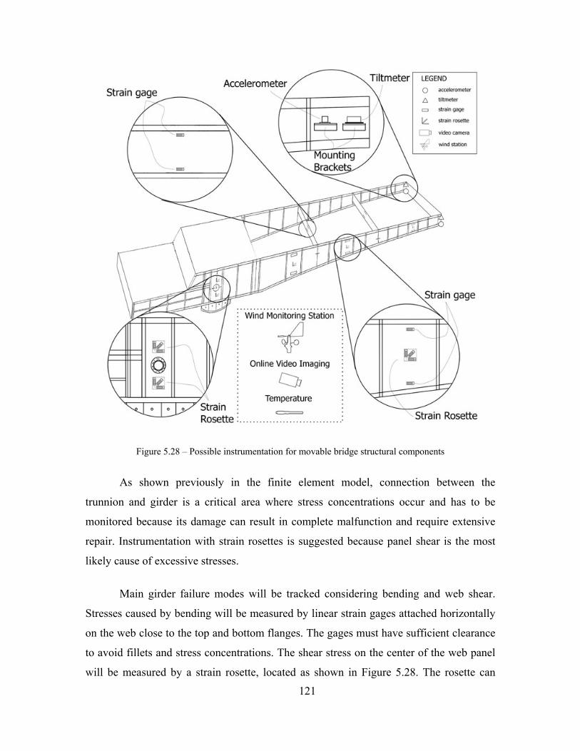
121
Figure 5.28 – Possible instrumentation for movable bridge structural components
As shown previously in the finite element model, connection between the
trunnion and girder is a critical area where stress concentrations occur and has to be
monitored because its damage can result in complete malfunction and require extensive
repair. Instrumentation with strain rosettes is suggested because panel shear is the most
likely cause of excessive stresses.
Main girder failure modes will be tracked considering bending and web shear.
Stresses caused by bending will be measured by linear strain gages attached horizontally
on the web close to the top and bottom flanges. The gages must have sufficient clearance
to avoid fillets and stress concentrations. The shear stress on the center of the web panel
will be measured by a strain rosette, located as shown in Figure 5.28. The rosette can

122
measure normal and shear strains in the plane of the gage, to be compared with the shear
capacity of the section.
Wind monitoring will be used for determining the input load on the structure
caused by air currents. Bascule bridges are slender and lightweight, and are significantly
affected by strong wind forces, especially when they are open. Measured wind speed and
direction will also be useful during hurricane-strength winds, indicating excessive force
on the girders. In addition to wind, ambient temperature and structural member
temperatures need to be monitored. Past studies have shown that temperature differentials
can cause considerably higher stresses than stresses induced by vehicular traffic (Catbas
and Aktan 2002). Finally, a video camera can be a complementary element as providing
vehicular traffic data to be correlated with other sensor readings, informing bridge
owners about accidents and suspicious activities. In addition, computer vision can be
employed for purposes such as tracking corrosion of the gears.
5.5. DATA PROCESSING AND SOME NEW ANALYSIS METHODS
For all options (Option A, B and C) explained in the previous section, data will be
collected by a data acquisition system installed at the bridge site. The data will be
analyzed at different levels to obtain information about the condition of the bridge. There
are different metrics (features) at each level of analysis and these metrics can be sent via
Internet connection to a main server to be stored. With the level of the analysis, the
complexity of analysis methods and algorithms increases accordingly. For example,
Level 1 refers to the raw data indicators and it represents the information obtained from
the raw data without detailed analysis. Then Level 2, which can be referred as
‘identification stage’, will be carried out by using different analysis methods and different
metrics to detect any damage, deterioration or ‘considerable change’ in measurements
over the monitoring period. Afterwards, more rigorous analysis will be conducted for
Level 3 to localize and quantify these ‘changes’, damage or deterioration. Finally, the
Level 4 will be used to predict the future behavior, as summarized in Table 5.1.
Table 5.1 Monitoring of the structure in different levels (some of the proposed metrics and methodologies)

123
Level 1 Level 2 Level 3 Level 4
Displacement,
Acceleration, Strain,
Rotation, Corrosion,
and Other Level 1
Measurements
Natural Frequency,
MAC, Statistical
Patterns such as
from Mah. Dis. of
the AR coefficients,
and Other Level 2
Methodologies
Flexibility,
Curvature,
Reliability Index,
and Other Level 3
Methodologies
Bayesian Updating,
and Other Level 4
Methodologies
Based on the instrumentation design and the data collection regime, it is possible
to collect, store and analyze various types of data sets. The writers’ experience is that this
process is rather iterative, especially at the early stages primarily influenced by the
preliminary evaluation of data. The writers propose the following for the movable
bridges: Maximum readings for each high speed gages such as strain gage and
accelerometer can be saved on hourly basis. To ensure that the entire time history is
captured, short duration windows of strain and acceleration are scanned for the peak
absolute values in each gage. If the peak absolute value for each gage exceeds the
previously recorded values for the current hour, the old peak time histories are
overwritten by the new ones. All sensor readings as well as temperature and wind speed,
and also a jpeg image from the video are recorded when a peak is detected. For long-term
monitoring, it is important to continuously monitor strain and temperature relationship
with a slower scan rate. Some of the critical components such as structural components
subjected to high stresses or stress reversals due to traffic or wind induced inputs, can be
monitored at different intervals or based on triggering.
At the end of each hour, the recorded data corresponding to peak values as well as
others can be loaded onto the main server through an Internet connection from the on-site
computer. The data from all gages are also recorded and transferred to the main server
when the measurements are above a threshold level. For the part of the instrumentation
application involving mechanical components, data can be recorded at the critical times
such as during opening and closing of the bridge leaves. For each opening/closing event,

124
shaft torsion, leaf angle, drive motor RPM and the video can be collected by the DAS,
transferred to the computer and archived in the main server.
Rotation at Tip
inTip Displacement Level
0.863
gAcceleration 0.255
Strain Near Trunnion
36.425 με
deg1.75
inCorrosion (Girder)
0.013
Green Yellow Red
Figure 5.29. Some of the proposed metrics for Level 1 monitoring (raw data indicators)
Figure 5.29 shows Level 1 monitoring with the raw data indicators. The on-site
computer will store only the designated long-term monitoring raw data such as slow
speed continuous strain-temperature or short duration high-speed vibration data. The rest
can be overwritten afterwards unless an operator decides to save the data. All processed
data and analysis results along with the designated raw data will be permanently stored.
As explained before, after Level 1 monitoring, different types of analyses can be
conducted. Several novel approaches and methodologies are being adapted, developed
and implemented by the UCF researchers to obtain the necessary useful information from
collected data. Some of these methodologies can be listed as statistical pattern
recognition approaches, parameter estimation by using model updating and optimization,
reliability based monitoring and the use of computer vision for structural health
monitoring. While the writers employ many different methods and approaches, brief
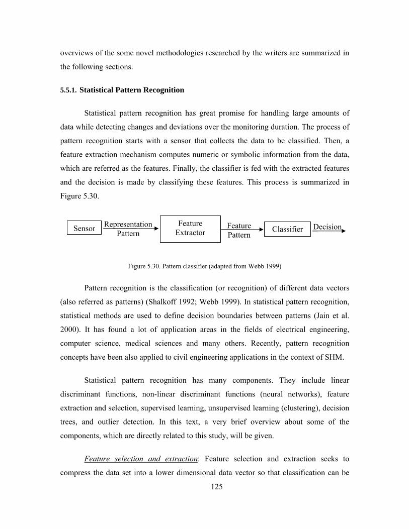
125
overviews of the some novel methodologies researched by the writers are summarized in
the following sections.
5.5.1. Statistical Pattern Recognition
Statistical pattern recognition has great promise for handling large amounts of
data while detecting changes and deviations over the monitoring duration. The process of
pattern recognition starts with a sensor that collects the data to be classified. Then, a
feature extraction mechanism computes numeric or symbolic information from the data,
which are referred as the features. Finally, the classifier is fed with the extracted features
and the decision is made by classifying these features. This process is summarized in
Figure 5.30.
Figure 5.30. Pattern classifier (adapted from Webb 1999)
Pattern recognition is the classification (or recognition) of different data vectors
(also referred as patterns) (Shalkoff 1992; Webb 1999). In statistical pattern recognition,
statistical methods are used to define decision boundaries between patterns (Jain et al.
2000). It has found a lot of application areas in the fields of electrical engineering,
computer science, medical sciences and many others. Recently, pattern recognition
concepts have been also applied to civil engineering applications in the context of SHM.
Statistical pattern recognition has many components. They include linear
discriminant functions, non-linear discriminant functions (neural networks), feature
extraction and selection, supervised learning, unsupervised learning (clustering), decision
trees, and outlier detection. In this text, a very brief overview about some of the
components, which are directly related to this study, will be given.
Feature selection and extraction: Feature selection and extraction seeks to
compress the data set into a lower dimensional data vector so that classification can be
Feature Pattern
Representation Pattern Sensor Feature
Extractor Classifier Decision

126
achieved. Obviously, the features should be selected very carefully so that maximum
separation can be achieved with the minimum number of features because the high
dimensional features often cause problems, which is also referred as ‘curse of
dimensionality’. Some of the features used for SHM are mentioned throughout this text.
Supervised Learning vs. Unsupervised Learning: The terms supervised and
unsupervised learning refer to the learning process when there is training data available
or not available respectively. Regression analysis (continuous data) and group
classification (discrete data) are types of supervised learning whereas clustering and
outlier analysis are often referred as unsupervised learning types. In SHM, the term
unsupervised learning implies that there is no available data from the damaged systems.
Figure 5.31 – Supervised and unsupervised learning for SHM
SHM as a Statistical Pattern Recognition Paradigm
Recently, a new definition of SHM was given by Sohn et al. (2001). The authors
stated that SHM is a statistical pattern recognition process and it is composed of the
following four portions.
Operational evaluation (how is damage defined, what are the conditions in the
operational environment, what are the limitations on acquiring data?)
Data acquisition (selecting the types, number and places of the sensors and defining
the other hardware, data normalization), data fusion (the integration of different sets
of data from different types of sensors) and cleansing (choosing the data to accept or
reject)
If data is available only from undamaged state
Unsupervised Learning
Clustering
If data is available from both damaged
and undamaged state
Supervised Learning
Regression Analysis

127
Feature extraction (identification of the metrics, which help to differentiate the
damaged and undamaged structure) and data compression
Statistical model development (models that will give the information about the
damage state of the structure by analyzing the identified features)
Statistical pattern recognition can be used for Level 2 monitoring through use of
many metrics as shown in Figure 5.32. There may be a number of metrics observed for
monitoring of the structure at this level and some examples are shown in Figure 5.32 as
natural frequency, Modal Assurance Criterion (MAC) and Mahalanobis distance (see
Appendix B) of the AR model coefficients. There are a number of examples showing
different methodologies for this type of monitoring, which can be addressed here.
However, for the sake of brevity, those which are directly related to this study will be
summarized in the following section. After this brief literature review, the studies
conducted by the authors will be discussed.
HzNatural Frequency
1.243
MAC 0.968
Mah. Dis. of the AR Coeff
3.214E4
Green Yellow Red
Figure 5.32. Some of the proposed metrics for Level 2 monitoring (identification of damage)
Sohn and Farrar (2001) used an Auto-Regressive (AR) model for estimating the
time history measurements from an undamaged structure. The AR coefficients of the
models fit to subsequent new data are monitored relative the control limits. In another
study, Sohn et al. (2001) applied two pattern recognition techniques to fiber optic strain
gauge data obtained from a surface-effect fast patrol boat. Recently, Dr. Catbas and his
students applied similar methodologies to identify different structural configurations of a

128
laboratory structure and details about this study is given in the Appendix B (Gul et al.
2007).
Worden (1997) used an Auto-Associative Network (AAN) for first level damage
detection. The feature for the network is selected as the transmissibility function between
two masses. More discussion about the applications of Neural Networks (NN) for
damage detection can be found in (Chen et al. 1995; Masri et al. 1996; Kao and Hung
2003). Worden et al. (2000) used outlier detection methods for damage identification and
applied it to four different cases. They also used Mahalanobis squared distance measure
for outlier detection.
Elimination of environmental effects from the data is another very important issue
and Principal Component Analysis (PCA) can be used for this purpose. PCA is a multi-
variate statistical method, also known as proper orthogonal decomposition. A very
attractive feature of the methodology is that environmental conditions do not need to be
measured for the analysis. Giraldo and Dyke (2004) applied the method to the ASCE
benchmark problem to identify damage under different environmental condition by using
computer simulations. Yan et al. (2005) verified the methodology by using experimental
data and applied it to real life data coming from Z24 Bridge in Switzerland. These
methodologies can be implemented at Level 2 monitoring to have more reliable
information about the changes in the data.
The authors implemented different algorithms and approaches to construct a novel
SHM methodology by using statistical pattern recognition. The theoretical background of
statistical pattern recognition based SHM and experimental studies conducted at UCF
Structures and System Research Laboratory are summarized in Appendix B. Figure 5.33
shows an example figure showing representative results of the statistical pattern
recognition applications on a steel grid structure where damaged structure state is
determined. Again, detailed information about the studies is given in Appendix B.

129
0 5 10 15 20 25 30 35 40 45101
102
103
104
105
106
107
108
Data Blocks
Mah
. Dis
. (lo
g)
HealthyDamaged
0 5 10 15 20 25 30 35 40 45101
102
103
104
105
106
107
10
Data Blocks
Mah
. Dis
. (lo
g)
HealthyDamaged
0 5 10 15 20 25 30 35 40 45
102
103
104
105
106
107
10
Data Blocks
Mah
. Dis
. (lo
g)
HealthyDamaged
0 5 10 15 20 25 30 35 40 45
102
103
104
105
106
107
10
Data Blocks
Mah
. Dis
. (lo
g)HealthyDamaged
Scour Damage Scenario
ThresholdDamageLocation
Figure 5.33 – Mahalanobis distance plots to detect damage case
5.5.2. Parameter Estimation with Sensor Fusion and Model Updating
After Level 2 monitoring, a more detailed and comprehensive analysis level can
be defined by using different approaches to SHM such as model updating using sensor
fusion, detailed modal analysis, Bayesian updating, computer vision and reliability
analysis. Some of the methodologies developed by the authors for condition assessment
of civil infrastructure can be found in literature (Catbas and Aktan 2002; Catbas et al.
2006). In this section, example studies regarding parameter estimation by using
optimization conducted at UCF Structures and Systems Research Laboratory will be
explained. Figure 5.34 shows some of the proposed metrics for Level 3 monitoring.

130
Reliability Index
in/kipFlexibility 0.432
1/inCurvature 0.255
kip/inBC (Spring Stiffness)
45.698
2.685
Green Yellow Red
Figure 5.34. Some of the proposed metrics for Level 3 monitoring (quantification and localization)
Parameter estimation is the procedure through which the unknown variables of an
analytical structure, whether stiffness, cross section area, elastic modulus or moment of
inertia or boundary condition stiffness, are updated using measured experimental
measurements. In real-world scenarios, structural member properties may differ from
their expected or “published” values due to variances from fabrication, construction or
destructive events such as damage or fatigue problems that occur over the service life of
the structure. Using optimization methods and experimental data sets, one can minimize
the error between the analytical and measured responses, updating the unknown
parameters. The updated model can then serve as a starting point, or baseline model for
future analysis and critical decision making (Francoforte et al. 2007). In the following
section the basic formulations are given without going into the details and example
studies conducted in UCF Structures and Systems Research Laboratory will be presented.
The classical matrix formulation for FEM force-displacement relationship is
{ } { }UKF ][= (5.1)
where { }F is force vector, { }U is vector of displacements and/or rotations and
[ ]K designates the structure stiffness matrix.

131
Since data over the entire set of degrees of freedom are generally not measured,
the formulation in above equation can be partitioned according to measured and
unmeasured DOF. Partitioning the force displacement relationship gives
⎭⎬⎫
⎩⎨⎧⎥⎦
⎤⎢⎣
⎡=
⎭⎬⎫
⎩⎨⎧
b
a
bbba
abaa
b
a
UU
KKKK
FF
(5.2)
where the subscripts a and b denote “measured DOF” and “unmeasured DOF”,
respectively.
By using static condensation, the analytically determined forces,{ }aF can be
solved in terms of the experimentally measured displacements and rotations, { }maU
where
{ } [ ] [ ][ ] [ ]( ){ } [ ][ ] { }bbbabababbabaaa FKKUKKKKF 11 −− +−= (5.3)
Since all of the unmeasured DOF are partitioned to{ }bF , part of the above
equation will be equal to a zero vector and cancel the multiplied sub matrices[ ]abK ,
[ ] 1−bbK if there is no force on the unmeasured DOF. Then, an error function can be
defined as the difference between the analytically determined forces, { }aF and the
experimental (applied) forces{ }m
aF , where { })(ke denotes the error as a function of the
unknown stiffness parameters and is given as
{ } [ ] [ ][ ] [ ]( ){ } [ ][ ] { } { }ma
mbbbab
mababbabaa FFKKUKKKKke −+−= −− 11)( (5.4)
By using similar approach the error function based on the difference between
analytically determined and experimentally measured displacements or rotations is
{ } [ ] [ ][ ] [ ]( ) { } [ ][ ] { }( ) { }ma
mbbbab
mababbabaa UFKKFKKKKke −−−= −−− 111)( (5.5)

132
Once test data are collected and the error functions are defined, an optimization
algorithm is required in order to minimize the error between the analytically determined
data and the experimental data. Optimization algorithms in general use iterative
approaches to determine the best or optimal solutions for a given set of equations. A
Spreadsheet Parameter Estimation (SPE) algorithm developed by Dr. Catbas and his
students is utilized for optimization of the error functions and for updating the unknown
stiffness parameters. The summary of the methodology is seen in Figure 5.35.
Figure 5.35 –General methodology for parameter estimation and model updating
A number of static and dynamic tests are conducted by using a simply supported
beam. More information about the beam and the sensor distribution on the beam can be
found in Appendix B. During the tests, different types of pads are used at the boundaries.
Then the SPE was used to identify the unknown stiffness parameters at the boundaries
and update the FEM. The following figure shows example results where five Duro50
pads were used at the boundaries. Then the stiffness parameters at the boundaries were
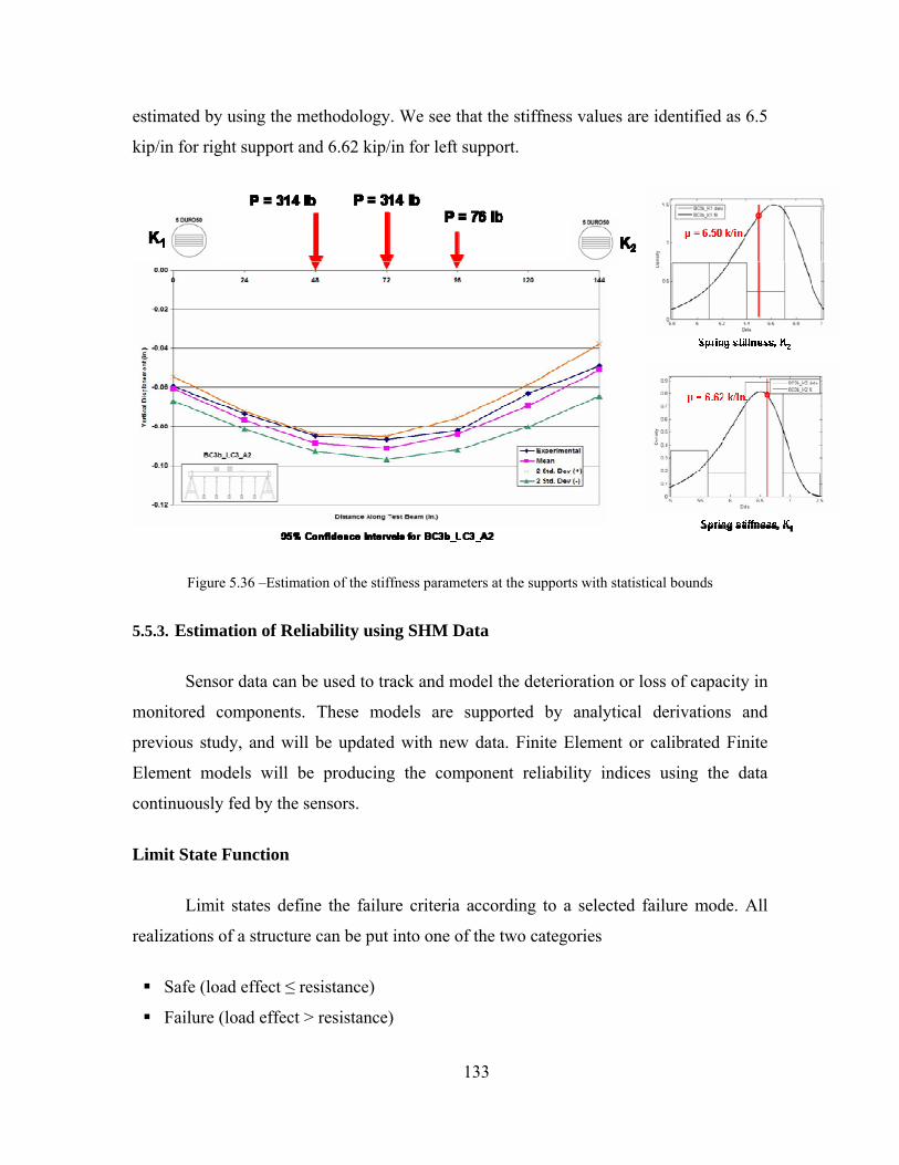
133
estimated by using the methodology. We see that the stiffness values are identified as 6.5
kip/in for right support and 6.62 kip/in for left support.
Figure 5.36 –Estimation of the stiffness parameters at the supports with statistical bounds
5.5.3. Estimation of Reliability using SHM Data
Sensor data can be used to track and model the deterioration or loss of capacity in
monitored components. These models are supported by analytical derivations and
previous study, and will be updated with new data. Finite Element or calibrated Finite
Element models will be producing the component reliability indices using the data
continuously fed by the sensors.
Limit State Function
Limit states define the failure criteria according to a selected failure mode. All
realizations of a structure can be put into one of the two categories
Safe (load effect ≤ resistance)
Failure (load effect > resistance)

134
The state of the structure can be described using parameters, X1, …,Xn where Xi’s
are load and resistance parameters
A limit state function is a function g(X1,…,Xn) of these parameters, such that
g(X1,…,Xn) ≥ 0 for a safe realization
g(X1,…,Xn)< 0 for failure
Each limit state function is associated with a certain limit state
Limit state functions are expressions defining the failure limit and generally in the
form of ( ) QRQRg −=, , i.e., they indicate the spare capacity of the structure or the
structural component. If the limit state function is positive, resistance is greater than the
load effects, so the structure is safe. If the limit state function is less than zero, this case
defines a failure since the load effect has exceeded the capacity. The curve or surface
defined by g = 0 is the failure surface dividing failure and survival spaces. Engineers’ aim
is always making g greater than zero, but how close to zero it may approach is related
with the balance between risk and cost (Ditlevsen and Madsen 1996; Melchers 1999;
Nowak and Collins 2000).
Reliability Index
Reliability index is a unit of failure probability, which is the area under the limit
state surface. In case a linear limit state function is considered;
( ) nnn XaXaXaaXXXg ++++= KK 2211021 ,,, (5.6)
Xi : uncorrelated random variables, with unknown types of distribution, but with
known mean values and standard deviations

135
Figure 5.37 – Limit state functions (Nowak and Collins 2000)
Then, the reliability index, β, can be calculated as follows,
( )∑
∑
=
=
+=
n
iXi
n
iXi
i
i
a
aa
1
2
10
σ
μβ (5.7)
Therefore, as shown in Figure 5.37, the reliability index for a linear limit state is
the shortest distance from the origin to the failure surface. If a non-linear limit state
function ( )nXXg ,,1 K is considered, then the limit state function can be linearized by
applying a Taylor series expansion and taking the first-order terms;
( ) ( ) ( )i
n
iiinn X
gxXxxgXXXg∂∂−+≈ ∑
=1
***121 ,,,,, KK
(5.8)
where the derivatives are calculated at (X1*, …, Xn*)
Component reliabilities can be generated with the sensor-based degradation
models for time functions of reliability. System reliability and component reliabilities can
be monitored real-time, and different alert levels can be triggered when a value below a
critical reliability index is calculated.

136
Prediction and Bayesian Updating
Bayesian updating technique is a very powerful tool to make use of new data to
refine the statistical parameters of an assumed or calculated distribution. The general
formula for Bayesian updating method is shown below;
( ) ( ) ( )( ) ( )∫
=θθθ
θθθdgxf
gxfxg||| (5.9)
where
( )xf |θ : conditional PDF of X given Θ (sampling distribution)
( )θg : PDF of Θ (prior distribution)
( )xg |θ : posterior PDF of Θ given x (posterior distribution)
θ : continuous parameter vector
x : sample data
Figure 5.38 – Concept of Bayesian Updating
This technique is previously used successfully to update condition state of bridges
when new visual inspection data is available. With time, the uncertainty of the estimated
parameters increases rapidly due to epistemic randomness, but using Bayesian updating,
new information is incorporated into the models to reduce that kind of uncertainty.
In the case of new monitoring data to be included in the existing knowledge, the
following simplified formula can be used for Bayesian updating:

137
( ) ( ) ( )θfx|θc·Lθf ΘΘ ′=′′
where
( )θ′Θf : prior distribution
( )x|L θ : likelihood function for Θ
( ) ( )[ ] 1−Θ∫ θθ′θ= dfx|Lc : normalizing factor to adjust the probability area
For the case where both ( )θ′f and ( )xf are normally distributed, the posterior
function ( )θ′′f is also normally distributed and has the mean value and standard
deviation, respectively, as
( ) ( )( ) ( )22
22
σ+σ′σμ′+σ′μ=μ ′′ ( ) ( )
( ) ( )22
22
σ+σ′σσ′
=σ ′′ (5.10)
where
σμ, : mean value and standard deviation of the a-priori distribution
σ′μ′, : mean value and standard deviation of the new data
σ ′′μ ′′ , : mean value and standard deviation of the updated distribution
If the distributions are non-normal, there may exist a closed form solution, but
otherwise, Monte Carlo simulation can be used to calculate the posterior distribution.
As an example study, the simply supported beam shown in Figure 5.15 is tested
for changing boundary conditions. Midspan displacement data was collected with a
displacement sensor for the different boundary conditions, which are pin-support, single
elastomeric pad and multiple elastomeric pads at the support locations, identical at both
sides. The aim is to simulate deteriorating support conditions and how these changes can
be tracked, translated into reliability analysis from monitoring data and future reliability
can be predicted.

138
P = 418 lb
P E = 29,000 ksi
Ix = 39.6 in4
pin i
single padl i d
L = 12 ft
a = 4 ft
different boundary conditions
Figure 5.39 – Simple beam test for Bayesian updating demonstration
The theoretical midspan displacement value for the given loading is taken as the
initial estimate of the displacement values. It is calculated according to the dimensional,
material properties and loading as; in.0450=δ (midspan deflection).
The theoretical displacement value will define the mean value of the existing
distribution, while uncertainty analysis needs to be conducted for defining the variability
of the distribution. However, for a demonstration, the initial displacement was assumed
to be normally distributed with a standard deviation of 0.001, to account for the
uncertainties due to unknown actual parameters.
Figure 5.40 – Test beam

139
Having the initial information, i.e., the a-priori condition, it is desired to integrate
the new data provided by sensor measurements. When new data is available, the previous
knowledge should not be discarded, but updated through Bayesian updating. Figure 5.17
shows the distributions of the previous data (theoretical displacement value) and the most
recent data (displacement gage at the midpoint for pinned end conditions).
In order to construct the reliability index, a limit state function needs to be
defined. Since the displacement is the main parameter in this particular example, the limit
state can be defined as the midspan deflection exceeding a pre-set value, which is set as
δmax = L/800.
( ) Δ −δ=Δ δ maxmaxdisp ,g (5.11)
which forms the reliability index as;
( ) ( )22Δδ
Δδ
σ+σ
μ−μ=β (5.12)
where Δ denotes the measured displacement
Figure 5.41 – Prior and new data for the test beam
The updating procedure generates the updated distribution, which involves less
uncertainty than both distributions, and its mean value is closer to the distribution with
higher confidence. Figure 5.24 shows the steps of updating the distributions with the

140
prior and recent information. On the right, the mean values are shown for the initial and
the following reliability points, before and after updating. With each new data set,
Bayesian updating is repeated, increasing the confidence of the data. Reliability indices
are calculated based on the defined limit state.
Figure 5.42 – Updating the available data and prediction with the first data set using Bayesian
The new data are incorporated into the previous data, creating a new distribution.
The figure on the right hand side shows the difference in the prediction curves for the
reliability index, based on curve fitting. The updated data also changes the curve fit,
hence the prediction of future performance.
Making predictions are the ultimate tools for decision making in bridge
management (Figure 5.43). The procedure will be applied to sensor data, which provides
more accurate information to fine-tune the prior distributions. This way, predictions will
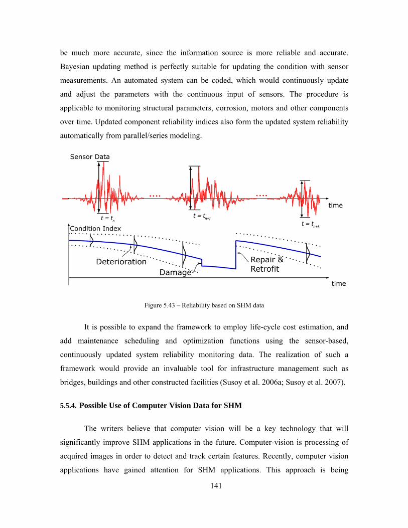
141
be much more accurate, since the information source is more reliable and accurate.
Bayesian updating method is perfectly suitable for updating the condition with sensor
measurements. An automated system can be coded, which would continuously update
and adjust the parameters with the continuous input of sensors. The procedure is
applicable to monitoring structural parameters, corrosion, motors and other components
over time. Updated component reliability indices also form the updated system reliability
automatically from parallel/series modeling.
Figure 5.43 – Reliability based on SHM data
It is possible to expand the framework to employ life-cycle cost estimation, and
add maintenance scheduling and optimization functions using the sensor-based,
continuously updated system reliability monitoring data. The realization of such a
framework would provide an invaluable tool for infrastructure management such as
bridges, buildings and other constructed facilities (Susoy et al. 2006a; Susoy et al. 2007).
5.5.4. Possible Use of Computer Vision Data for SHM
The writers believe that computer vision will be a key technology that will
significantly improve SHM applications in the future. Computer-vision is processing of
acquired images in order to detect and track certain features. Recently, computer vision
applications have gained attention for SHM applications. This approach is being

142
implemented and improved at the UCF Structures and Systems Research Laboratory
where a novel framework for real-life structures is being constructed. Basic methodology
of the framework and preliminary results are described as follows;
Video streams are used in conjunction with computer vision techniques to
determine the class, speed, and location of vehicles moving over the bridge. A database is
constructed using information from the vehicles (loads) training sets, the experimental
results from the sensors network and a finite element model. Then, this proposed system,
by interpreting the images and correlating those with the information contained in the
database, will evaluate the operational condition of the bridge.
All of this will be done in real time, without the necessity of processing large
amounts of data after its acquisition. Additionally, video can be used to detect suspicious
activities, i.e. the presence of persons, vehicles and/or objects in critical or prohibited,
predetermined locations. Every day, at every moment, the bridge will be monitored and
its condition will be assessed, preventing further damage and catastrophes and keeping
the most critical legacy data, for further studies.
Figure 5.44 – Computer vision integration into SHM

143
The system will provide real-time continuous assessment: video cameras will be
detecting, tracking, and classifying vehicles permanently, and sensors will be
synchronized with the video input to detect the structural behavior. This feature will help
prevention of catastrophic failures, notification of any abnormal behavior, generation of
image and numerical records, remote visual monitoring, tracking of structural behavior
and help in scheduling condition-based maintenance. The integration of computer vision
into a SHM system is illustrated in Figure 5.44.
Identifying moving objects from a video sequence is a critical task for all vision
systems. Some kind of mechanism is required to detect what is happening in the field of
view of the camera. Any moving or out-of-place object is noted and has to be somehow
detected. Once objects are detected, further processing is needed to indicate in which
direction they are moving (tracking) and/or what kind of object is (classification). A
common approach for identifying the moving objects is background subtraction, where
each video frame is compared against a reference or background model. Pixels in the
current frame that deviate significantly from the background are considered to be moving
objects and belonging to the foreground. This pixel-based information is then clustered to
identify regions in order to label, and classify objects.
Detection previously obtained will include false positives due to a variety of
reasons. For example, background moving objects (leaves and branches, debris, shadows,
occlusions, etc.) be considered foreground objects, leading to false results. To eliminate
this identity mistakes data must be validated. The most common approach is to combine
morphological filtering and connected components grouping to eliminate these regions.
Connected component grouping is used to identify all regions that are connected and
eliminates those that are too small to correspond to real interest moving points. In this
way, the remaining noise is eliminated.
A bounding box is drawn around the object and its size (number of pixels) and
centroid (location within the image) are calculated. Once each vehicle/object is detected
and located in the image, its image coordinates have to be converted and mapped into the
real world coordinates system. This is achieved by finding the intrinsic and extrinsic

144
camera parameters that establish the relationship between image (I) and world (W)
coordinates. These parameters were found by knowing a set of points in the image and
real world, establishing a system of equations and using singular value decomposition to
get the final solution. This procedure is explained schematically in Figure 5.45.
{ }∑∑= =
=n
i
m
jijijijnxm BGR
NBGR
1 1
,,1},,{
{ } { } { }∑∑= =
−=n
i
m
jijijijnxmnxmBGR BGRBGR
N 1 1
2, ,,,,1, σσσ
BACKGROUND MODEL
MEAN
STANDARD DEVIATION
{ }
TT
MbMgMr
IbIgIr
xbgr
xMbMgMr
IbIgIr
⎪⎭
⎪⎬
⎫
⎪⎩
⎪⎨
⎧−
⎪⎭
⎪⎬
⎫
⎪⎩
⎪⎨
⎧
⎪⎭
⎪⎬
⎫
⎪⎩
⎪⎨
⎧−
⎪⎭
⎪⎬
⎫
⎪⎩
⎪⎨
⎧=Δ
σσσ1
INPUT FRAME
THRESHOLD Δ>λ CONNECTED COMPONENTS FILTERING DETECTION
NORMALIZED DIFFERENCE
TRUCK TYPE 1:
2 AXLES
Dimensions=
Min Load=
Max Load=
CLASSIFICATION
⎥⎥⎥⎥
⎦
⎤
⎢⎢⎢⎢
⎣
⎡
⎥⎥⎥⎥
⎦
⎤
⎢⎢⎢⎢
⎣
⎡
⎥⎥⎥
⎦
⎤
⎢⎢⎢
⎣
⎡−
−=
⎥⎥⎥
⎦
⎤
⎢⎢⎢
⎣
⎡
1100001000000
3,32,31,3
3,22,21,2
3,12,11,1
world
world
world
z
y
x
yy
xx
image
image
ZYX
trrrtrrrtrrr
ofkofk
SVU
TRACKING/MAPPING IMAGE-WORLD COORDINATES
CORRELATION
• REAL-TIME VIDEO
• SENSORS READINGS
ASSESSMENT/DIAGNOSTIC
{ }∑∑= =
=n
i
m
jijijijnxm BGR
NBGR
1 1
,,1},,{
{ } { } { }∑∑= =
−=n
i
m
jijijijnxmnxmBGR BGRBGR
N 1 1
2, ,,,,1, σσσ
BACKGROUND MODEL
MEAN
STANDARD DEVIATION
{ }
TT
MbMgMr
IbIgIr
xbgr
xMbMgMr
IbIgIr
⎪⎭
⎪⎬
⎫
⎪⎩
⎪⎨
⎧−
⎪⎭
⎪⎬
⎫
⎪⎩
⎪⎨
⎧
⎪⎭
⎪⎬
⎫
⎪⎩
⎪⎨
⎧−
⎪⎭
⎪⎬
⎫
⎪⎩
⎪⎨
⎧=Δ
σσσ1
INPUT FRAME
THRESHOLD Δ>λ CONNECTED COMPONENTS FILTERING DETECTION
NORMALIZED DIFFERENCE
TRUCK TYPE 1:
2 AXLES
Dimensions=
Min Load=
Max Load=
TRUCK TYPE 1:
2 AXLES
Dimensions=
Min Load=
Max Load=
CLASSIFICATION
⎥⎥⎥⎥
⎦
⎤
⎢⎢⎢⎢
⎣
⎡
⎥⎥⎥⎥
⎦
⎤
⎢⎢⎢⎢
⎣
⎡
⎥⎥⎥
⎦
⎤
⎢⎢⎢
⎣
⎡−
−=
⎥⎥⎥
⎦
⎤
⎢⎢⎢
⎣
⎡
1100001000000
3,32,31,3
3,22,21,2
3,12,11,1
world
world
world
z
y
x
yy
xx
image
image
ZYX
trrrtrrrtrrr
ofkofk
SVU
TRACKING/MAPPING IMAGE-WORLD COORDINATES
⎥⎥⎥⎥
⎦
⎤
⎢⎢⎢⎢
⎣
⎡
⎥⎥⎥⎥
⎦
⎤
⎢⎢⎢⎢
⎣
⎡
⎥⎥⎥
⎦
⎤
⎢⎢⎢
⎣
⎡−
−=
⎥⎥⎥
⎦
⎤
⎢⎢⎢
⎣
⎡
1100001000000
3,32,31,3
3,22,21,2
3,12,11,1
world
world
world
z
y
x
yy
xx
image
image
ZYX
trrrtrrrtrrr
ofkofk
SVU
TRACKING/MAPPING IMAGE-WORLD COORDINATES
CORRELATION
• REAL-TIME VIDEO
• SENSORS READINGS
ASSESSMENT/DIAGNOSTIC
Figure 5.45 – SHM and computer vision integrated operation

145
Moving objects in two consecutive frames are matched allowing the calculation
of its speed while moving along the bridge. v = d/t where v represents the speed, d is the
distance between centroids of the same object for the two images, and t is the elapsed
time between images (1/30 s. for two consecutive frames is the standard frame capture
ratio for the type of camera used). To actually track a vehicle thru the video constrains
like maximum speed, common motion, and minimum velocity are used. Additional
information provided by color and size allows the building of an index-weighted matrix,
which provides the most probably matching objects between the two frames. Estimation
of the next position of the vehicle (centroid) is found. This value is fundamental when
correlating sensor readings vs. load positions.
Finally, once an input is received from the vision module, the system will infer
the structure health by comparing the expected results for those loads (from the database)
with the actual readings (from the sensors array). Surveillance capabilities could also be
added to discern between normal and suspicious activities and emit alerts if needed.
The proposed framework will also be capable of maintaining a permanent
surveillance for safety monitoring. Video surveillance and monitoring is a rapidly
growing area of video computing, particularly for suspicious activities, accidents and
threats. The objectives of video surveillance and monitoring systems are to (1) detect
moving objects in the video, (2) track objects throughout the sequence, (3) classify them
into people, vehicles, animals, etc., and (4) recognize their activities. The system will be
able to inform the bridge owner and/or other agencies in possible cases of accidents,
pedestrians, overloads, suspicious activities including non-moving vehicles, persons
around certain locations, presence of objects left on critical locations, etc (Zaurin and
Catbas 2007).
5.6. DATA MONITORING FRONT PANEL
An integrated monitoring system has been set up in the UCF Structures and
Systems Research Laboratory, which allows monitoring various sensor data and video
images. The front panel of the data acquisition system is shown in Figure 5.46. The
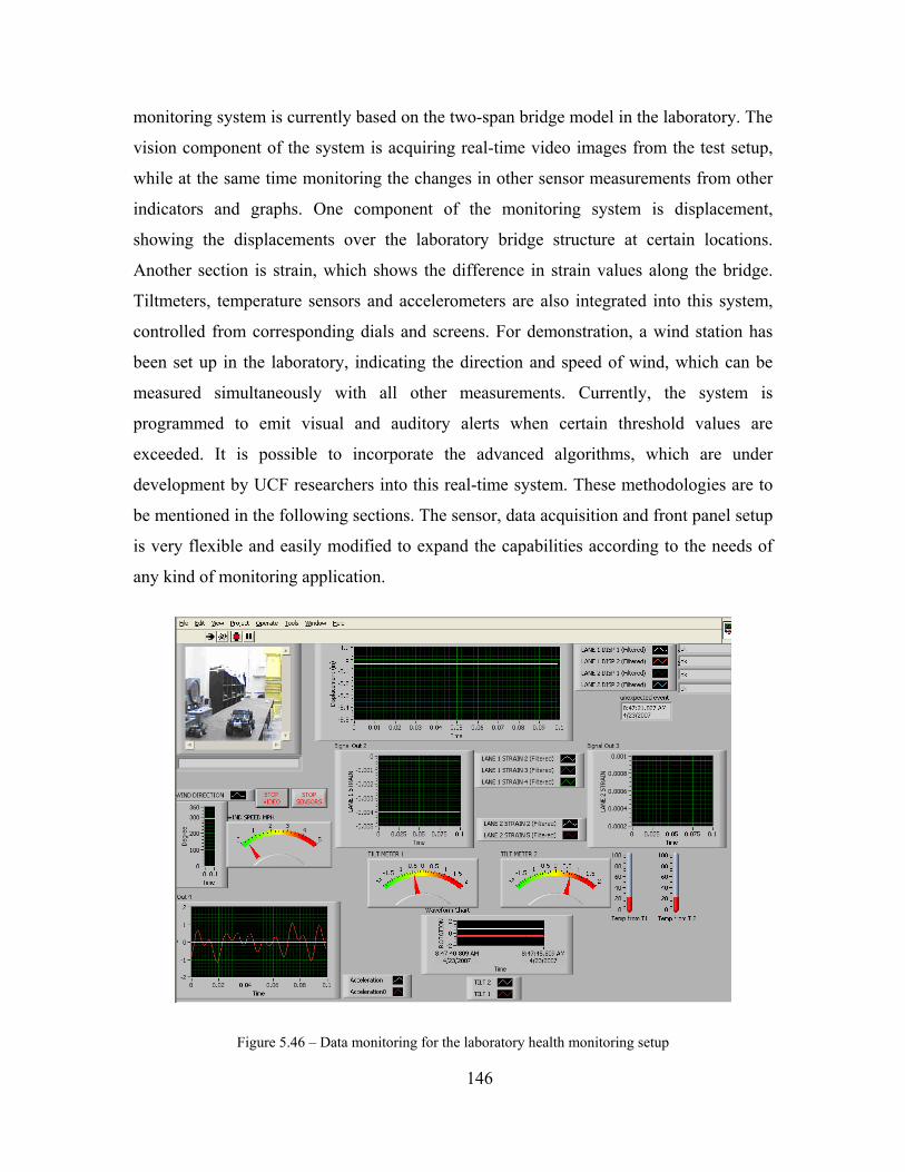
146
monitoring system is currently based on the two-span bridge model in the laboratory. The
vision component of the system is acquiring real-time video images from the test setup,
while at the same time monitoring the changes in other sensor measurements from other
indicators and graphs. One component of the monitoring system is displacement,
showing the displacements over the laboratory bridge structure at certain locations.
Another section is strain, which shows the difference in strain values along the bridge.
Tiltmeters, temperature sensors and accelerometers are also integrated into this system,
controlled from corresponding dials and screens. For demonstration, a wind station has
been set up in the laboratory, indicating the direction and speed of wind, which can be
measured simultaneously with all other measurements. Currently, the system is
programmed to emit visual and auditory alerts when certain threshold values are
exceeded. It is possible to incorporate the advanced algorithms, which are under
development by UCF researchers into this real-time system. These methodologies are to
be mentioned in the following sections. The sensor, data acquisition and front panel setup
is very flexible and easily modified to expand the capabilities according to the needs of
any kind of monitoring application.
Figure 5.46 – Data monitoring for the laboratory health monitoring setup

147
A modified version of the existing monitoring system is proposed for day-to-day
applications of actual bridges for the use of engineers and, if required, the public with
various levels and limitations as illustrated in Figure 5.47. The sensor arrays and data
acquisition systems of the framework should be tailored for the specific needs of the
monitored bridge. The system, after collecting the data, should process the data at the
server nodes supporting a database structure.
The main server can provide physical storage for the post-processed and filtered
data, as well as other archived inspection and maintenance reports. The information on
the main server can be accessible through the web. Security of the system is very critical
since the bridges as well as the management system are important assets. Access to the
database should be limited by defining users with passwords and their position, task and
privileges. So, only certain sections of the database should be allowed to each user.
Figure 5.47 – Movable bridge remote monitoring system

148
Additionally, real-time data monitoring will be provided. The real-time mode
displays data from any sensors at a particular location and live video streaming will be
available. Streaming data can be observed by an authorized user from any remote site
equipped with Internet access.
5.7. DATA MANAGEMENT AND INFORMATION TECHNOLOGIES
In the following schema, integration of Bridge Health Monitoring (BHM) and
Bridge Management System (BMS) is illustrated. Sensors on the structure transmit
signals to the data acquisition stations through wired or wireless connections, according
to the SHM design. Raw data delivered by data acquisition stations are processed and
converted into meaningful data, which is then logged into the database. Inspection reports
from visual inspection of the structure are also added to the database in electronic format.
Then, the integrated database containing bridge information, legacy data and condition
state serves as a hub for all offices and districts for reaching, updating and sharing this
information.
Figure 5.48 - Database implementation
Advantages of utilizing the Internet for bridge management and database
applications are numerous. A system working on Internet will be much more convenient

149
for the users, who will have access with any kind of Internet connection. There will be no
compatibility issues or installation and maintenance of software for each user, since
regular internet browsers will be enough for all tasks. Intra-agency information sharing
and collaboration is also maximized.
A typical database for SHM can be composed of three conceptual layers, each of
which is associated with certain functions of its mechanism. These are;
1. Data Layer
2. Business Layer
3. Presentation (Client) Layer
An example of a database working schema is given in Figure 5.49.
Figure 5.49 - Database functional layers
The data layer is static, representing stored physical data. The data layer is the
foundation of the database, containing all data and tables. This layer is at the background
and accesses only through the business layer. The business layer contains the rules,
policies and algorithms for manipulating the data layer. Algorithms that determine the
reliability indices from SHM data and store into appropriate fields/tables in the database

150
are parts of the business layer. The client layer is the interface that the user uses to
interact and to send and receive information. When the user requests bridge network
monitoring or life-cycle cost optimization display from the client layer, the business layer
retrieves the necessary information from the data layer, converts into required format, and
sends to the client layer for display.
Figure 5.50 – Example framework for internet-based database
This database structure also allows life-cycle maintenance cost analyses using
bridge deterioration models and effects and unit costs associated with each action.
Optimum maintenance plans will be drawn for a given bridge lifetime, minimizing the
total cost and assuring certain safety levels. This will be an ultimate tool for high-level
management of bridges, allowing trade-off analysis and budget decisions with maximum
efficiency.

151
6. CONCLUSIONS AND RECOMMENDATIONS
This study aims to provide a general Structural Health Monitoring (SHM)
framework to be applied for improved decision making for managing bridges. In the
study, the components of an SHM system that are discussed include instrumentation, data
collection, advanced techniques that enable high-level analysis and presentation of
collected data, and data archival and management using information technology.
Movable bridges in Florida are selected as the focus of this project, due to their different
maintenance needs, and significantly higher maintenance costs than fixed highway
bridges, making them a more critical bridge population and good candidates for
monitoring.
6.1. CONCLUSIONS AND FINDINGS
From analysis of movable bridge records, inspection reports, and site visits, the
movable bridge population is identified to have a high deterioration rate for structural
components. Structural components are subject to corrosion and adverse effects due to
misalignments and operational wear. In addition, the mechanical and electrical systems
are subject to frequent problems or breakdowns even if they are continuously inspected
and maintained.
Among the FDOT movable bridge inventory, Christa McAuliffe Movable Bridge
in Merritt Island, on SR-3 is selected as an average bridge according to the general
characteristics, such as age, size, type and operation frequency. This bridge is assumed to
be representative of most of the movable bridges in Florida, which have similar
characteristics. In-depth analysis of the inspection reports over a 25 year period is
conducted. It is seen that the orthotropic deck, movable components such as shafts,
emergency drives, and locks and live load shoes exhibit low condition ratings. As a
result, this bridge was rehabilitated twice in the 1990s. It is also observed that while
rehabilitation improved the condition ratings, some components such as span lock ratings
dropped shortly after the rehabilitation. In addition to the inspection results, finite
element analyses are prepared and presented to help understand the critical response

152
locations and levels. The models are used to determine operating levels of stresses and
deflection under various load conditions. The tip deflection under single AASHTO
HL-93 truck and two HL-93 trucks+lane load are determined to be 1.65 in and 4.49 in,
respectively. The serviceability limit for this bridge and deck type is determined to be 5.6
in. The maximum stresses under dead load and two HL-93 trucks+lane load around
trunnion, at span lock and live load shoe are determined to be ~6-12 ksi, ~10 ksi, ~15 ksi,
respectively. The frequencies and mode shapes are also sensitive to damage, imbalance
and structural changes. For example, it is seen that additional modes appear when span
lock failure is simulated. For the undamaged condition, the first three modes are at 3.69
Hz, 4.74 Hz and 9.04 Hz. The load rating is determined to be lowest right above the love
load shoes. The inventory and operating rating values under two HL-93 trucks+lane load
at this location are 0.98 and 1.27, respectively. However, it is seen that under one HL-93
truck traveling at 50 mph, the lowest system reliability index is determined to be 5.79
which is far above the 3.5 (AASHTO LRFD for new design) and 2.5 (AASHTO LRFR
for existing bridges). These results are valuable to determine the monitoring locations,
sensing requirements and expected ranges. Analyses based on finite element modeling of
this bridge, inspection data and data collection from balance tests revealed that the
complex structural, mechanical and electrical systems are very sensitive to maintenance
neglects, therefore, need to be monitored closely.
6.2. INSTRUMENTATION PLAN
A proposed instrumentation plan on structural components, which would enable
tracking of the current condition and deterioration, is presented. The proposed SHM
instrumentation is based on site visits and meetings with several maintenance and repair
engineers at different districts, analysis of inspection records, and analytical models and
simulations. The following are found to be candidates for instrumented monitoring, in
addition to various common structural components:
Electrical Motors
Gear Boxes
Open Gears / Racks
Hopkins Frame
Trunnions
Live Load Shoes
Span Locks

153
Issues associated with these components and possible monitoring solutions are
documented in the report. The main purpose of the instrumentation plan is to provide a
better tracking system of maintenance issues, which would increase the maintenance
efficiency and indicate critical service needs to reduce breakdowns.
A major benefit of a monitoring system is that any sudden change in the capacity
or partial/total collapse of a bridge can be detected and “seen” instantly. Especially after a
catastrophic natural or man-made event, such as hurricane, or vessel/vehicle impact, rapid
condition evaluation of bridges is imperative. During or in the aftermath of a widespread
disaster, such a system would be the key for strategic emergency response operations, by
determining whether the bridges are operational, critically damaged, or failed. This will
allow the establishment of safe routes as well as the prioritizing of emergency repair
operations.
Coupled with appropriate sensors and sensing networks, advanced analysis
techniques such as statistical pattern recognition methodologies, reliability based
monitoring, and computer vision oriented SHM enable processing of data for generating
useful information through a series of algorithms. The aim is to provide useful
information quickly, and these methodologies are currently in development to indicate
the condition scientifically, detect anomalies and damage, and provide predictions and
future trends based on the results extracted from collected data. Problems caused by
physical scatter and discrepancy of current data collection and storage systems can be
overcome by establishing an innovative mechanism of information management system
where all the data is collected in standard formats and transferred to a central database,
where raw and processed data are logged and stored. This database is to serve all clients
of different layers within the organization up to the level of their involvement with the
information and authorization by the system. In addition to serving as a data terminal, the
system can provide means of efficient communication among all branches in lateral and
vertical dimensions.

154
6.3. RECOMMENDATIONS AND FUTURE STUDY
For a complete Structural Health Monitoring system, the integration of the
monitoring components is necessary. Remote monitoring and integrated data archival
methods are presented to make the maximum and most efficient use of the collected data.
Based on the framework defined in this report, it is possible to build a monitoring system
for a movable bridge that covers whole aspects from sensor installation to user controls.
The proposed instrumentation plan was aimed at addressing maintenance,
operation and safety issues, and leading to more efficient management practices for
movable bridges. A continuous monitoring system, with relatively little investment, can
help track the bridges’ degradation. Therefore, projections for the structural performance
can be made over the long-term and preventative maintenance work can be better
scheduled. In addition, this approach should eliminate or significantly reduce unexpected
breakdowns by providing instant warnings to maintenance personnel. Proactive
maintenance is a much more efficient practice than repairing the bridge after extensive
damage is discovered, or in case of a breakdown, which prompts costly and time-
consuming emergency repairs. Costs associated with traffic delays will also be reduced.
We note that the integrated monitoring framework proposed in this report is developed in
parallel to efforts of the Federal Highway Administration Long Term Bridge
Performance Program (LTBPP). The LTBPP focuses on continuous bridge monitoring
applications for developing improved knowledge on performance and degradation, better
design methods and performance predictive models, and advanced management decision-
making tools.In light of the findings from the current studies, it is recommended that
complete SHM systems are adapted and implemented to complement current bridge
management systems. An application such as described in this report is expected to
mitigate the problems and reduce maintenance costs. Further studies and pilot
applications are necessary to test and evaluate new technologies and algorithms as well as
to quantify the cost-benefit ratio of integrated SHM applications. This way, the approach
can be further improved and customized according to user needs and other challenges
that can only be discovered through real-life applications.

155
7. REFERENCES
"Manual for Maintenance Inspection of Bridges", AASHTO, 1983.
"Guide Manual for Condition Evaluation and Load and Resistance Factor Rating (LRFR)
of Highway Bridges, 1st Edition", AASHTO, 2003a.
"Manual for Condition Evaluation and Load and Resistance Factor Rating (LRFR) of
Highway Bridges" American Association of State Highway and Transportation
Officials, AASHTO, 2003b.
"Development of a Model Health Monitoring Guide for Major Bridges" Drexel
Intelligent Infrastructure and Transportation Safety Institute, Aktan, A. E., Catbas, F.
N., Grimmelsman, K. A. and Pervizpour, M., 2003.
Aktan, A. E., Chase, S., Inman, D. and Pines, D. (2001a). "Monitoring and Managing the
Health of Infrastructure Systems". Proceedings of the 2001 SPIE Conference on
Health Monitoring of Highway Transportation Infrastructure, Irvine, CA, March 6-8.
Aktan, A. E., Pervizpour, M., Catbas, F. N., Grimmelsman, K. A., Barrish, R. A., Curtis,
J. and Qin, X. (2001b). "Information Technology Research for Health Monitoring of
Bridge Systems". Proceedings of the Structural Faults & Repair 2001 Conference,
London, UK, July 4-6, 2001.
"AASHTO LRFD Bridge Design Specifications" Washington, DC., American
Association of State Highway and Transportation Officials (AASHTO), 2002.
Anderson, O. D. (1976). "Time Series Analysis and Forecasting the Box-Jenkins
Approach." Butterworth & Co, UK.
Asmussen, J. C. (1997). "Modal Analysis Based on the Random Decrement Technique -
Application to Civil Engineering Structures." Doctoral Dissertation, University of
Aalborg, Aalborg.

156
"Parametric Finite Element Modeling and Full-Scale Testing of Trunnion-Hub-Girder
Assemblies for Bascule Bridges" A Report on a Research Project Spnsored by the
Florida Department of Transportation, Besterfield, G., Kaw, A. and Crane, R., 2001.
Box, G. E., Jenkins, G. M. and Reinsel, G. C. (1994). "Time Series Analysis: Forecasting
and Control". Prentice-Hall, New Jersey.
Burkett, J. L. (2005). "Benchmark Studies for Structural Health Monitoring using
Analytical and Experimental Models." MS Thesis, Department of Civil and
Environmental Engineering, University of Central Florida, Orlando, FL.
Buxton-Tetteh, B. (2004). "Development of User Cost Model for Movable Bridge
Openings in Florida." MS Thesis, Civil Engineering, Florida State University,
Tallahassee, FL.
Catbas, F. N. and Aktan, A. E. (2002). "Condition and Damage Assessment: Issues and
Some Promising Indices." Journal of Structural Engineering, ASCE, 128(8): 1026-
1036.
Catbas, F. N., Brown, D. L. and Aktan, A. E. (2006). "Use of Modal Flexibility for
Damage Detection and Condition Assessment: Case Studies and Demonstrations on
Large Structures." Journal of Structural Engineering, ASCE, 132(11): 1699-1712.
Catbas, F. N., Ciloglu, S. K. and Aktan, A. E. (2005). "Strategies for Condition
Assessment of Infrastructure Populations: A Case Study on T-beam Bridges."
Structure and Infrastructure Engineering Journal, SIE, 1(3): 221-238.
Catbas, F. N., Shah, M., Burkett, J. and Basharat, A. (2004). "Challenges in Structural
Health Monitoring". Proceedings of the 4th International Workshop on Structural
Control, 195-202, Columbia University, New York, June 10-11.
Chen, H. M., Qi, G. Z., Yang, J. C. S. and Amini, F. (1995). "Neural Network for
Structural Dynamic Model Identification." Journal of Engineering Mechanics, ASCE,
121(12): 1377-1381.

157
Ditlevsen, O. and Madsen, H. O. (1996). "Structural reliability methods". Wiley,
Chichester ; New York.
Dunn, P. F. (2005). "Measurement and Data Analysis for Engineering and Science".
McGraw-Hill, New York, NY.
"Structures Design Guidelines" Florida Department of Transportation, FDOT, 2004.
"Recording and Coding Guide for the Structural Inventory and Appraisal of the Nation's
Bridges" FHwA, Federal Highway Administration (FHWA), 1995.
"Transportation Asset Management Case Studies, FHWA-IF-05-040: Bridge
Management Experiences of California, Florida, and South Dakota" Office of Asset
Management, Federal Highway Administration (FHWA), 2005.
"Transportation Asset Management Case Studies, Bridge Management: Experiences of
California, Florida and South Dakota", FHWA, 2003.
"Bridge Inspector's Reference Manual" Publication No. FHWA NHI 03-001, FHWA
Report, 2002.
Francoforte, K., Gul, M. and Catbas, F. N. (2007). "Parameter Estimation Using Sensor
Fusion and Model Updating". Proceedings of the 25th International Modal Analysis
Conference (IMAC), Orlando, FL, February 19 - 22.
Giraldo, D. and Dyke, S. J. (2004). "Damage Localization in Benchmark Structure
Considering Temperature Effects". 7th International Conference on Motion and
Vibration Control.
Gul, M. and Catbas, F. N. (2006). "An Integrated System Identification Framework for
Structural Condition Assessment Using Ambient Vibration Data." Journal of
Engineering Mechanics, ASCE, under review.

158
Gul, M., Catbas, F. N. and Georgiopoulos, M. (2007). "Application of Pattern
Recognition Techniques to Identify Structural Change in a Laboratory Speciment".
Proceedings of the SPIE Smart Structures and Materials & Nondestructive Evaluation
and Health Monitoring Conference San Diego, CA, March 18 - 22.
Jain, A. K., Duin, R. P. W. and Mao, J. (2000). "Statistical Pattern Recognition: A
Review." IEEE Transactions on Pattern Analysis and Machine Intelligence, 22(1): 4-
37.
Jain, A. K., Murty, M. N. and Flynn, P. J. (1999). "Data Clustering: A Review." ACM
Computing Surveys, 31(3): 264-323.
Kao, C. Y. and Hung, S.-L. (2003). "Detection of Structural Damage via Free Vibration
Responses Generated by Approximating Artificial Neural Networks." Computers and
Structures, 81: 2631-2644.
Koglin, T. L. (2003). "Movable Bridge Engineering". John Wiley and Sons.
Lynch, J. P. and Loh, K. (2005). "A Summary Review of Wireless Sensors and Sensor
Networks for Structural Health Monitoring." Shock and Vibration Digest, Sage
Publications, 38(2): 91-128.
"Handbook of Bascule Bridge Balance Procedures" Report submitted to Florida
Department of Transportation, Malvern, L. E., Lu, S. Y. and Jenkins, D. A., 1982.
Masri, S. F., Nakamura, M., Chassiakos, A. G. and Caughey, T. K. (1996). "Neural
Network Approach to Detection of Changes in Structural Parameters." Journal of
Engineering Mechanics, ASCE, 122(4): 350-360.
Melchers, R. E. (1999). "Structural Reliability Analysis and Prediction". John Wiley &
Sons.
Nair, K. K. and Kiremidjian, A. S. (2005). "A Comparison of Local Damage Detection
Algorithms Based on Statistical Processing of Vibration Measurements". Proceedings

159
of the 2nd International Conference on Structural Health Monitoring and Intelligent
Infrastructure (SHMII), Shenzen, China.
Nowak, A. S. (1995). "Calibration of LRFD Bridge Code." ASCE Journal of Structural
Engineering, 121(8): 1245-1251.
Nowak, A. S. and Collins, K. R. (2000). "Reliability of Structures". McGraw-Hill.
Omega Engineering Inc. (1995). WMS-22A and WMS-22 Current Loop Wind Stations:
Operator's Manual.
Patton, G. C. (2006). "Bascule Leaf Fabrication and Erection Tolerances: Where
Structure Meets Machine". Heavy Movable Structures, Inc. Eleventh Biennial
Symposium, Orlando, FL.
"Bridge Analysis and Rating Program - BAR7, V7.10" PennDOT Bureau of Information
Systems Application Development Division, PennDOT, 2001.
"Remote Global Monitoring of the Michigan Street Bridge, Sturgeon Bay, Wisconsin"
ITI technical report no. 19, Prine, D. W. and Fish, P. E., 1996.
Rackwitz, R. and Fiessler, B. (1978). "Structural Reliability under Combined Random
Load Sequences." Computers and Structures, 9: 489-494.
Shalkoff, R. J. (1992). "Pattern Recognition: Statistical and Neural Approaches". John
Wiley & Sons, US.
Sohn, H. and Farrar, C. R. (2001). "Damage Diagnosis Using Time Series Analysis of
Vibration Signals." Smart Materials and Structures, 10: 1-6.
Sohn, H., Farrar, C. R., Hunter, N. F. and Worden, K. (2001). "Structural Health
Monitoring Using Statistical Pattern Recognition Techniques." Journal of Dynamic
Systems, Measurement, and Control, 123: 706-711.

160
Susoy, M., Catbas, F. N. and Frangopol, D. M. (2006a). "Implementation of Structural
Reliability Concepts for Structural Health Monitoring". Proceedings of the 4th World
Conference on Structural Control and Monitoring, San Diego, CA, July 11-13.
Susoy, M., Catbas, F. N. and Frangopol, D. M. (2006b). "Reliability-Based SHM of a
Long-Span Bridge." Journal of Engineering Structures, Elsevier (submitted).
Susoy, M., Catbas, F. N. and Frangopol, D. M. (2007). "Structural Health Monitoring
Development using System Reliability". Proceedings of the 10th International
Conference on Applications of Statistics and Probability in Civil Engineering
(ICASP10), University of Tokyo, Japan, July 31 - August 3.
Thompson, P. D., Sobanjo, J. O. and Kerr, R. (2003). "Florida DOT Project-Level Bridge
Management Models." Journal of Bridge Engineering, ASCE, 8(6).
"Bridge Study Analyzes Accuracy of Visual Inspections"
http://www.tfhrc.gov/focus/jan01/bridge_study.htm, Turner-Fairbank Highway
Research Center, 2005.
"Bridge Study Analyzes Accuracy of Visual Inspections"
http://www.tfhrc.gov/focus/jan01/bridge_study.htm, Turner-Fairbanks Highway
Research Center, 2005.
Webb, A. (1999). "Statistical Pattern Recognition". Oxford University Press, New York,
NY.
Wong, K.-Y. (2005). "Design of Structural Health Monitoring System for Long-Span
Bridges." Structure and Infrastructure Engineering, 3(2): 169-185.
Worden, K. (1997). "Structural Fault Detection Using a Novelty Measure." Journal of
Sound and Vibration, 201(1): 85-101.
Worden, K., Sohn, H. and Farrar, C. R. (2000). "Damage Detection Using Outlier
Analysis." Journal of Sound and Vibration, 229(3): 647-667.

161
Worden, K., Sohn, H. and Farrar, C. R. (2002). "Novelty Detection in a Changing
Environment: Regression and Interpolation Approaches." Journal of Sound and
Vibration, 229(3): 647-667.
Xu, R. and Wunsch, D. (2005). "Survey of Clustering Algorithms." IEEE Transactions
on Neural Networks, 16(3): 645-678.
Yan, A.-M., Kerschen, G., De Boe, P. and Golinval, J.-C. (2005). "Structural Damage
Diagnosis under Varying Conditions - Part I: A Linear Analysis." Mechanical
Systems and Signal Processing, 19: 847-864.
Zaurin, R. and Catbas, F. N. (2007). "Computer Vision Oriented Framework for
Structural Health Monitoring of Bridges". Proceedings of the 25th International Modal
Analysis Conference (IMAC), Orlando, FL, February 19 - 22.

162
APPENDIX A. SENSORS AND DATA ACQUISITION SYSTEMS
A.1. SENSOR TECHNOLOGY
Sensing technology is advancing very rapidly, allowing networks of large
numbers of sensors to be deployed practically and with relatively low cost. Many new
types of sensors are now available for various types of applications. Sensors are now used
in almost all fields and industries, from medical to aerospace. Introduction of wireless
transmission for sensor signals made a huge impact on the feasibility of instrumentation
applications by reducing the cost and trouble of installing the cables and wires for large-
scale projects.
A.2. GENERAL TYPES OF SENSORS
Strain Gage
The strain gage is one of the most widely used strain measurement sensors. It is a
resistive elastic unit whose change in resistance is a function of applied strain. Strain
gages measure the expansion and contraction of material due to mechanical stress or
thermal effect. Like all transducers, these sensors rely on indirect measurements for
determining strains. Two common sensor types are the electrical resistance strain gage
and the fiber optic strain gage.
The metallic foil-type strain gage consists of a grid of wire filament (a resistor) of
approximately 0.001 in. (0.025 mm) thickness, bonded directly to the strained surface by
a thin layer of epoxy resin. Their rugged construction and flexibility make them suitable
for static and dynamic measurement with a high degree of accuracy. The measuring grid
is formed by etching Constantan foil, which is then completely sealed in a carrier
medium composed of polyimide film.
When a load is applied to the surface, the resulting change in surface length is
communicated to the resistor and the corresponding strain is measured in terms of the
electrical resistance of the foil wire, which varies linearly with strain. The foil diaphragm

163
and the adhesive bonding agent must work together in transmitting the strain, while the
adhesive must also serve as an electrical insulator between the foil grid and the surface.
When selecting a strain gage, one must consider not only the strain characteristics
of the sensor, but also its stability and temperature sensitivity. Unfortunately, the most
desirable strain gage materials are also sensitive to temperature variations and tend to
change resistance as they age. For tests of short duration, this may not be a serious
concern, but for continuous, long-term monitoring applications, one should include
temperature and drift compensation.
Bonded resistance strain gages have been proven to be reliable. They are
relatively inexpensive, can achieve overall accuracy of better than +/-0.10%, are available
in a short gage length, are only moderately affected by temperature changes, have small
physical size and low mass, and are highly sensitive. Bonded resistance strain gages can
be used to measure both static and dynamic strains. This is the type of strain gage used in
the demonstration study of movable bridge instrumentation.
Strain Rosette
A wire strain gage can effectively measure strain in only one direction. To
determine the three independent components of plane strain, three linearly independent
strain measures are needed, i.e., three strain gages positioned in a rosette-like layout.
Figure A.1 – A strain rosette
The following coordinate transformation equation is used to convert the
longitudinal strain from each strain gage into strain expressed in the x-y coordinates,

164
(A.1)
Applying this equation to each of the three strain gages results in the following
system of equations,
(A.2)
These equations are then used to solve for the three unknowns, εx, εy, and εxy. For
the example case study presented in the following sections, 45º strain rosette aligned with
the x-y axes, i.e., α = 0º, β = γ = 45º, for which the following set of equations are used for
calculating the plane strains;
⎪⎪
⎩
⎪⎪
⎨
⎧
ε+ε−ε=ε
ε=εε=ε
2ca
bxy
cy
ax
(A.3)
Vibrating Wire Strain Gages
Vibrating wire gages operate by generating a 'current pulse' to excite or 'pluck' the
wire in the vibrating wire gauge. Immediately following excitation, the resonant
frequency of the vibrating wire is measured. The pulse has a current source characteristic
that provides automatic cable length compensation. Sensors on long cables will be pulsed
with the similar energy as those on shorter cables. Produced frequency signal is measured
by a precision frequency counter.

165
Any deformation of the vibrating wire changes its natural frequency, which may
be expressed as:
mF
L21fw
= (A.4)
where Lw is the length of wire; F is the tension on the wire; and m is the mass per
unit length for the wire. Expressing mass, m in terms of material density, ρ, cross-
sectional area, a, and gravitational acceleration, g, the equation will yield:
agF
L21fLa
g·LWm
ww
w ρ=⇒ρ== (A.5)
Expressing the tension force, F, in terms of strain:
ρε
=⇒ε=gE
L21faEF w
ww (A.6)
where E is the Young’s modulus, and εw is the strain in the wire.
Inserting the specified parameter values of the vibrating wire material
(E = 30×106 psi, ρ = 0.283 lb/in3, g = 386 in/s2):
wwL
101142f ε= (A.7)
and 2
2w
wT
L75.97=ε (A.8)
Therefore, with this equation, the strain is related to the natural period of the wire.
Since the signal is in terms of frequency, there is no loss of signal while traveling along
long cables.
Arc-weldable and spot-weldable versions are available for easy mounting on steel
surfaces. These gages can also be used on concrete, by using studded end-blocks, which

166
are embedded into the concrete. Vibrating wire strain gages are very stable and durable.
The advantage of vibrating wire gages over resistance-based gages is their self
temperature compensation making them more suitable for long-term measurements.
However, their sampling rate is rather slow, therefore, dynamic events such as traffic and
vibration cannot be measured.
Accelerometer
With strain gages, accelerometers are the most commonly used sensor in
structural monitoring. A brief summary of the most common accelerometer types is
presented and their inherent benefits/drawbacks summarized.
Force balance accelerometers are spring mass devices which feature high
sensitivity over a relatively low frequency range. The ability to make low frequency
measurements with high accuracy makes this class of accelerometers particularly well
suited for seismic and general structural monitoring applications. Because of their
exceptional resolution, this class of accelerometer became the standard for permanent
structural monitoring systems. However, due to their high costs and evolving sensor
technologies, other types of accelerometers are becoming more popular.
Piezoelectric accelerometers incorporate a crystal sensing element which has the
property of emitting a charge when subjected to a force. As these are active electrical
systems, the crystals produce an electrical output only when they experience a change in
load, they cannot perform true static measurements. Typical piezoelectric accelerometers
offer higher measurement and frequency ranges than force balance accelerometers at the
expense of resolution and inability to measure down to 0 Hz. Lower costs are another
advantage of piezoelectric accelerometers over FBA’s.
Capacitive accelerometers measure acceleration by monitoring a change in
electrical capacitance. Within these sensors, the sensing element consists of two parallel
plate capacitors acting in a differential mode. These capacitors operate in a bridge circuit,
along with two fixed capacitors, and alter the peak voltage generated by an oscillator
when the structure undergoes acceleration. Like the force balance accelerometer,

167
capacitive accelerometers typically operate in a low frequency range. Unlike
piezoelectric accelerometers, these sensors can measure down to 0 Hz. The principal
advantage of capacitive accelerometers is their low cost, making them attractive for dense
sensor arrays; however, the resolution of these sensors is typically less than either force
balance or piezoelectric accelerometers.
Wind
Wind plays a major role on the movable bridges, due to their relatively slender
structure. The leaves sustain significant wind loading especially when open and the
mechanical drive system opening and closing them is also affected. An inexpensive
option for these measurements is the WMS-22B series sensor capable of monitoring wind
speed and direction at discrete locations on a bridge. The WMS-22 Current Loop Wind
Station measures wind speed and direction and converts each parameter into 4 to 20mA
output signals for use by process control or monitoring systems. No external power is
required since the encoding electronics for wind speed and for wind direction are isolated
and powered form their respective 2-wire current loops (Omega Engineering Inc. 1995).
These stations are capable of measuring wind speed from 1 to 136 miles-per-hour (mph)
with 1 mph resolution. For wind direction, the station offers 0º to 360º capability with 2º
resolution.
Displacement
The most basic type of these devices measure displacement via a flexible cable
that extracts from and retracts to a spring-loaded drum. They convert mechanical motion
into electrical signals that can be measured. An internal spring helps maintain tension on
the cable and the threaded drum rotates a precision rotary sensor that produces an
electrical output proportional to the cable travel. These displacement transducers are
very easy to configure, setup and make measurements. The advantages of using these
sensors are that they are easy to install, cost effective, reliable and have minimal signal
conditioning requirements.

168
Tiltmeters
Tiltmeters measure the change of inclination of a surface or a component. They
usually encompass a pendulum mass; therefore, rotation of the device induces spring
forces due to earth’s gravitation. Tiltmeters might be based on electrical resistance or
vibrating wire principles, similar to strain gages.
Vibrating wire tiltmeters are also comprised of a pendulous mass, which is under
the force of gravity. As tilt increase or decreases, the mass attempts to rotate beneath the
elastic hinge point and the tension in the vibrating wire changes, altering the natural
frequency. Like the vibrating wire strain gages, an electromagnetic coil plucks the
vibrating wire in order to read the natural frequency. Some advantages of using vibrating
wire tiltmeters is that they combine high range with high sensitivity, and have excellent
long-term stability. Since the sensor outputs readings in units of frequency, there is little
attenuation over long cable lengths.
A.3. DATA ACQUISITION SYSTEMS CURRENTLY IN USE AT THE UCF STRUCTURES AND
SYSTEMS RESEARCH LABORATORY
Various data acquisition devices and systems are currently in use and/or being
tested in the UCF Structures and Systems Research Laboratory.
A.3.1. VXI SYSTEM
An acquisition system from VXI and Agilent technologies is currently being used.
From the accelerometers, the continuous electrical signal is conditioned before being
discretized into finite values by the digitizer. After the signal is digitized, the PC link
enables the data to be stored to the computer.
There are two cards that plug into the VXI mainframe. As mentioned previously
one is the digitizer and the other links to the PC via IEEE 1394 fire wire. Currently, the
digitizer card is limited to 16 channels but provides similar constraints to real-life
monitoring whereby instrumentation must be limited due to time and economic reasons.

169
One of the most powerful aspects of this digitizer and acquisition system is that all the
time data is collected simultaneously as opposed to a finite difference in each channels
recording history. In addition to collecting data, the PC link card is also used as the
controller for the electro-seis shaker. The shaker cable connects to the PC link and then
the settings are configured with the testing software.
Figure A.2 – Signal conditioning
A.3.2. NATIONAL INSTRUMENTS SYSTEM
There are many advantages to using a DAQ system from National Instruments
(NI). As stated before, health-monitoring systems may require integration of multiple
DAQ systems in order to run different sensors that may not work on a particular DAQ.
The following components are available in the laboratory, which are sufficient for
building a data acquisition network:
SCXI 1001 chassis
SCXI-1520 universal strain gage
module
SCXI-1314 terminal input block
PXI 1033 chassis
PXI 6221 controller card
Labview software

170
Figure A.3 – National Instruments system in the laboratory; (a) SCXI 1001 chassis, (b) PXI 1033 chassis
One SCXI-1520 universal strain gage module is to be inserted into one of the free
slots on the SCXI 1000 chassis. The 1520 module is pre-wired to accommodate a wide
variety of strain gages.
A.3.3. CAMPBELL SCIENTIFIC
The Campbell Scientific datalogging equipment used in the laboratory includes
the following:
CR10X datalogger
AM16/32 Multiplexer
AVW1 Vibrating Wire Gage Interface
PS100 12V Power Supply
The CR10X is a rather inexpensive and robust data collection unit, found
extensively in environmental and civil monitoring applications. The CR10X datalogger is
a rugged unit capable of running in some of the most demanding environments, and in
temperatures ranging from -25˚C to +50˚C. The unit has 2 Mbytes of internal storage
capacity, allowing for up to 524,288 data values per MByte, where high-resolution data
(5 decimal characters) equals 4 bytes and low-resolution data (4 decimal characters)
equals 2 bytes. The CR10X is capable of sampling rates from real-time to 64Hz and up
to 750Hz using burst measurements over short intervals. Analog inputs allow for 6

171
differential or 12 single ended measurements, as well as accommodations for resistance
measurements (resistive bridge-based), as well as excitation outputs of -2.5V to +2.5V.
Because it is relatively inexpensive, up to 4 multiplexers can be used with one
CR10X datalogger, allowing hundreds of sensors to be run at a time. Two separate
modes, “2x32” and “4x16” allow for scanning of 32 sensor input channels, each having 2
lines and for scanning of 16 sensor input channels, each having 4 lines respectively. The
maximum number of sensors that can be multiplexed is limited to: 32 single-ended or
differential analog sensors not requiring excitation (thermocouple) or 16 single-ended or
differential sensors requiring excitation (full bridge strain gages). In a differential
measurement, the voltage on the H input is measured with respect to the voltage on the L
input. A single-ended measurement is used to measure voltage at a single-ended input
with respect to ground. Although often used in conjunction with the CR10X, the
multiplexer is only good for indoor, non-condensing environments. Separate enclosure
units can be purchased to protect the system if it is used outdoors. Like the CR10X, the
AM16/32 can be used in temperatures ranging from -25˚C to +50˚C.
A.3.4. OTHER DATA ACQUISITION SYSTEMS
One of the emerging technologies in the field of health monitoring today is the
use of wireless communication systems to measure and record field data. Wireless
devices such as sensors allow measurements to be made from remote locations without
the need for long cables. By reducing the need for cables running from the sensor to the
DAQ, overall costs of the health monitoring system can be greatly reduced. Wireless
sensors may also be used in locations that would otherwise be inaccessible, if using
conventional gages. The system we have is comprised of 3-USB base stations, 4 V-Link
wireless DAQ transceivers and 2 G-Link wireless accelerometer systems from
Microstrain, Inc.
The V-Link wireless transceivers feature bridge completion, on board sensor
excitation, programmable offsets and gains, and differential and single ended inputs.
Samples can be triggered and stored on the onboard 2 Mbytes flash memory or streamed

172
real-time from up to 200 feet away. Its rechargeable battery system allows for ~230
hours on continuous operation. These units feature a sweep rates from 32 Hz (slow-
speed) up to 2 KHz (high-speed). An integrated analog to digital converter allows for 12
bits resolution of data. Each V-Link transceiver is programmed to communicate with a
base station running at 925 MHz frequency.
Figure A.4 – Microstrain data acquisition and transmitter

173
APPENDIX B. RELATED LABORATORY STUDIES
The Structures Laboratory of the University of Central Florida is capable of
accommodating various types of experimental studies. The laboratory has also been a test
bed for investigating, installing and developing sensing systems and analysis methods of
structures based on monitoring data.
Shown below is an instrumentation study on a steel beam, on which strain,
displacement, accelerometer, and tilt measurements via different sensor types were
employed.
Figure B.1 – Test beam

174
Figure B.2 – Some tests performed on the test structure
The aim of the tests was to check the sensors and data acquired before deploying
them in the field for monitoring actual structural components, and also, to develop and
enhance current analysis techniques by comparing test results to mathematical and finite
element models. From comparative analysis results, it was seen that experimental
parameters are in a good correlation with the updated FEM.
Figure B.3 – Analysis results from the instrumented beam

175
Another significant test setup in the laboratory is the grid structure. This structure
is being used to conduct monitoring tests, in which this structure is modified to represent
single-span or double-span bridges, or run damage scenarios.
Figure B.4 – Grid structure in the laboratory
Among many results obtained from the numerous test on this structure, a couple
of them show that damage can be detected by using sensor networks and developed
analysis techniques.
Figure B.5 – Results of dynamic analysis and damage scenarios

176
Statistical Pattern Recognition Applications to SHM
In the literature, statistical pattern recognition has generally been used in
conjunction with time series modeling of structural response data. Auto-Regressive
models are highly utilized for this purpose. After constructing the AR models of the time
history data, the model coefficients are used as damage indicating features. Then any
statistical pattern recognition algorithms can be applied by using these features.
The researchers have implemented pattern recognition algorithms to identify
damage in different test specimens. One example is given here to show the methodology
implemented by the authors. After giving the overview of the methodology, discussions
about the algorithms applied are given in the following sections without going into the
details.
The analysis procedure applied in this study is similar to the approach used by
Sohn et al. (2001) in the sense that AR model coefficients are used as features for outlier
detection. However, in this analysis Random Decrement (RD) is applied to each channel
to normalize the data before constructing the Auto Regressive (AR) models. After
normalizing (averaging) the data using RD, AR models are fitted to the averaged data.
Then the coefficients of these models are used as the damage indicating features and they
are fed to the outlier detection and clustering algorithms (Figure B.6).

177
AR
Mod
elR
D
Set ofFeatures
X=[x1 x2 … xn]
x1 x2xn
Am
bien
t A
ccel
erat
ion
… … …
… … …
RD
RD
… … …
AR
Mod
el
AR
Mod
elFeat
ures
Ave
rage
d D
ata
Figure B.6 – General Methodology
Random Decrement: The basic idea behind the method will be briefly
summarized in the following paragraph, however more comprehensive information can
be found in Asmussen (1997). Moreover, detailed discussions about its application for
ambient data analysis is given in Gul and Catbas (2006) where the authors combined
Complex Mode Indicator function (CMIF) with RD method to extract several features,
such as modal frequencies, mode shapes, scaled and pseudo flexibilities, from ambient
test data.

178
The random response of a system at a particular time consists of three
components, which are the step response due to the initial displacements, the impulse
response from initial velocity, and a random part due to the load applied to the structure.
By taking the average of data segments, every time the response has an initial
displacement bigger than the trigger level, the random part due to random load will
eventually vanish and become negligible. Additionally, since the sign of the initial
velocity can be assumed varying randomly in time, the resulting initial velocity will also
be zero, leaving a pseudo-free response of the system (Asmussen 1997).
Time Series Analysis - Auto Regressive (AR) Model: Time series analysis is a
common method for novelty detection applications to detect damage (Sohn and Farrar
2001; Sohn et al. 2001; Worden et al. 2002; Nair and Kiremidjian 2005). AR, ARX and
ARMA (Auto-Regressive Moving Average) models were some of the time series analysis
methods employed in that studies. Here, brief descriptions about the theory behind AR
modeling will be presented. Preliminary results related to the AR modeling are presented
in the following sections.
An AR model estimates a function’s value at time t based on a linear
combination of prior values. The model order (generally shown with p ) determines the
number of past values, which will be used to estimate the value at t (Anderson 1976).
The basic formulation of a p order AR model is defined as follows.
)()()(1
tetitxtxp
ii +Δ−=∑
=
φ (B.1)
The identification of the model requires determining the unknown coefficients of
the AR model by using the data points. The AR coefficients can be computed in different
ways. The coefficients can be computed from autocorrelation estimates, from partial
autocorrelation coefficients, and from least-squares matrix procedures. In this text, the
least square formulation will be given as an example. The formulation is summarized in
the following paragraph.

179
Let us assume there are m data points. Then, the following set of linear equations
can be written by using 1−m blocks of data, which consists of 1+p data points.
[ ]{ } { }xx
x
xx
xxx
xxxxxx
m
p
p
p
p
mpmpm
p
p
=⇒
⎪⎪⎭
⎪⎪⎬
⎫
⎪⎪⎩
⎪⎪⎨
⎧
=
⎪⎪⎭
⎪⎪⎬
⎫
⎪⎪⎩
⎪⎪⎨
⎧
⎥⎥⎥⎥⎥
⎦
⎤
⎢⎢⎢⎢⎢
⎣
⎡
+
+
−
−+−−
+ φ
φ
φφ
MM
L
MOMM
L
L
2
1
1
1
11
132
21
(B.2)
To solve the unknown coefficients,
{ } [ ] [ ]( ) [ ]{ }xxxx T 1−=φ (B.3)
Here, [ ] [ ]( ) [ ]xxx T 1− is so called pseudo inverse (note that [ ]x is not necessarily
square) of [ ]x and the unknown coefficients can in fact be considered as least square
solution.
A very crucial point here is the determination of the model order. Among many
model order determination criteria, partial auto-correlation can be applied to determine
the model order. For this study, the partial auto-correlation function is defined as the last
AR coefficient (Box et al. 1994). To determine the model, the partial auto-correlation
function is calculated for increasing p values and the correct model order is set to the p
value whose auto-correlation function value is under a pre-set threshold value.
Clustering and Outlier Detection: Clustering can be described as defining groups
in the data set where the data points in the same groups (clusters) are similar to each other
and dissimilar to the data points in the other clusters. More details about the topic and
different clustering approaches can be found in the studies by Jain et al. (1999) and Xu et
al. (2005).
K-means clustering is a very simple, yet powerful, unsupervised learning
algorithm to cluster a given data set. The basic idea behind the method is to define k
clusters in the data set by minimizing the following objective function

180
∑∑= =
−=k
j
n
ij
ji cxV
1 1
)( (B.4)
where )( jix is ith data point in cluster j and jc is the center of the cluster j. First, an
initial partition with k clusters is selected. Then new partitions are generated by assigning
each data point to its closest cluster. Afterwards, new clusters are recorded and the
centers of the new clusters are calculated. This procedure is repeated until the cluster
membership is stabilized (Jain et al. 2000).
Outlier detection, however, is detection of clusters, which deviate from other
clusters so that they are assumed to be generated by another system or mechanism.
Outlier detection is one of the most common pattern recognition concepts, which is
applied to SHM problem as mentioned in detail in the previous sections of this text.
Therefore, a special emphasize will be put on outlier detection.
The outlier detection problem for univariate (1D) data is relatively straightforward
meaning that the outliers must be removed from one end or the other of the data set
distribution. There are several discordance tests but one of the most common is based on
deviation statistics and it is given by the following
σξ
ξ
xxz
−= (B.5)
where ξx is the potential outlier and x and σ are the sample mean and standard
deviation, respectively. The multivariate equivalent of this discordance test is known as
the Mahalanobis squared distance and given as
)()( 1 xxxxZ T −Σ−= −ξξξ (B.6)
where ξx is the potential outlier vector and x is the mean vector and Σ is the
sample covariance matrix. By using the above equations, the outliers can be detected if
the Mahalanobis distance of a data vector is bigger than a pre-set threshold level. The
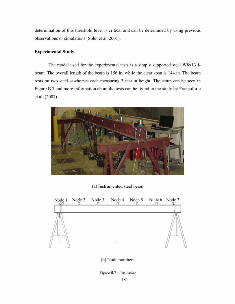
181
determination of this threshold level is critical and can be determined by using previous
observations or simulations (Sohn et al. 2001).
Experimental Study
The model used for the experimental tests is a simply supported steel W8x13 I-
beam. The overall length of the beam is 156 in, while the clear span is 144 in. The beam
rests on two steel sawhorses each measuring 3 feet in height. The setup can be seen in
Figure B.7 and more information about the tests can be found in the study by Francoforte
et al. (2007).
(a) Instrumented steel beam
(b) Node numbers
Figure B.7 – Test setup

182
Although it is a simple laboratory specimen, a very interesting, if not unique,
aspect of this study is that the beam is densely instrumented with a number of sensors and
is tested for many different structural configurations (different boundary conditions). The
total number of dynamic and static sensors is 29 (seven accelerometers, seven
displacement gages, seven tiltmeters and eight strain gages); however only the results
obtained with data coming from accelerometers will be presented in this text.
The Boundary Conditions (BC) of the structure are modified by changing the
material that sits on the support (between the sawhorses and the beam). The material can
be a neoprene pads (different configurations of two types of pads) or a steel angle.
Although a number of BC is applied during the tests, only four of them are used in this
study and they are summarized in Table B.7.1. It should be noted that the first BC is also
referred as the baseline case throughout the text.
Table B.7.1 – The BC applied to the test beam
Name Boundary Condition
BC1 Pin supports at each support
BC2 4 Duro50 pads at node 1; Pin/shims at node 7
BC3 5 Duro50 pads at each support
BC4 5 Duro70 pads at each support

183
Figure B.8 – Example pictures showing different BC (a) The pin support for BC1
(b) Four Duro50 pads for BC2 (c) Five Duro70 pads for BC4
Please note from Figure B.8(a) that the accelerometers are not placed exactly on
the supports. The reason for this is that the accelerometers were positioned right above
the displacement gages and the displacement gages could not be placed under the
supports. So, when the term ‘support points’ is used in the following sections, the reader
should understand ‘the points at the vicinity of the supports’. Figure B.8(b) and Figure
B.8(c) show some of the other BC.
Framework of the Analysis and Results: As explained before, the ambient data is
first processed (averaged) by using the random decrement method. A pseudo-free
response of the system is obtained when RD is applied to data. Then, the AR models are
fitted to the averaged data to obtain the damage indicating features (please refer to Figure
B.6).
There are a number of different crucial parameters for the analysis such as the size
of the data blocks, the reference channel for RD and the model order of AR models. A
sensitivity analysis concerning these parameters can reveal important information,
however, it is beyond the scope of this study. The ambient data is collected from each
channel for approximately 10 minutes with a sampling frequency of 800 Hz. 18 blocks
with 50000 points with no overlap are used for each BC. Reference channel for RD is
node 2 and each data block has 1024 points after averaging with RD. The model order p
for AR models is 10 and obtained by using partial auto-correlation function (Box et al.
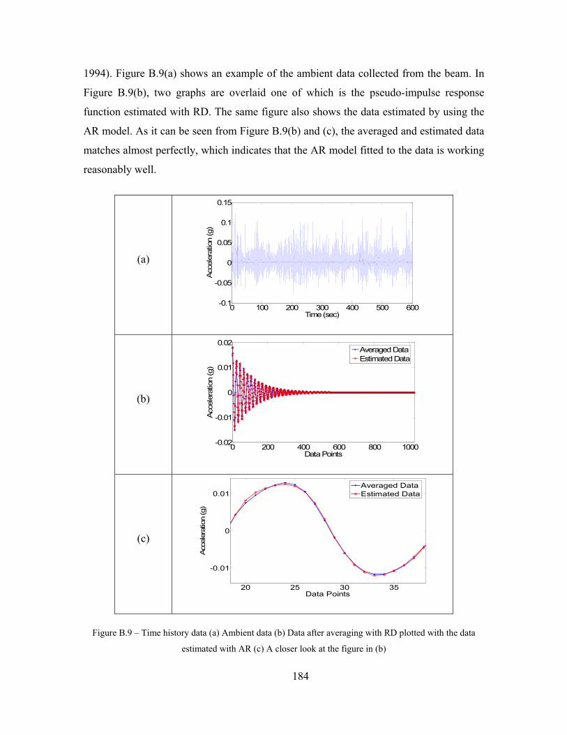
184
1994). Figure B.9(a) shows an example of the ambient data collected from the beam. In
Figure B.9(b), two graphs are overlaid one of which is the pseudo-impulse response
function estimated with RD. The same figure also shows the data estimated by using the
AR model. As it can be seen from Figure B.9(b) and (c), the averaged and estimated data
matches almost perfectly, which indicates that the AR model fitted to the data is working
reasonably well.
(a)
0 100 200 300 400 500 600-0.1
-0.05
0
0.05
0.1
0.15
Time (sec)
Acc
eler
atio
n (g
)
(b)
0 200 400 600 800 1000-0.02
-0.01
0
0.01
0.02
Data Points
Acc
eler
atio
n (g
)
Averaged DataEstimated Data
(c)
20 25 30 35
-0.01
0
0.01
Data Points
Acc
eler
atio
n (g
)
Averaged DataEstimated Data
Figure B.9 – Time history data (a) Ambient data (b) Data after averaging with RD plotted with the data
estimated with AR (c) A closer look at the figure in (b)

185
After constructing the AR models, the coefficients of these models are used as the
damage indicating features. Please note that, for each BC, there are 18 data blocks, which
means there are 18 sets of feature vectors each containing 10 AR coefficients. Then, all
of these features are used to calculate the Mahalanobis distance between the features
coming from different BC. The same features are also fed to K-Means to see if the data
coming from different BC can be clustered properly.
Figure B.10 compares the features coming from BC1 and BC2 for the seven
nodes. The first half of the features (blue stars) is coming from BC1 whereas second half
of them (red circles) represents the BC2. It is clearly seen from Figure B.10(a) that the
two BC can be well separated by using Mahalanobis distance. However, Figure B.10(b)
shows that the same BC cannot be differentiated with the same features by using K-
Means clustering. Mahalanobis distance works also quite well for classifying BC1 and
BC3 as it is shown in Figure B.10(c). Unlike the previous case, K-Means works
reasonably good for these cases (Figure B.10(d)) yet it does not perform as well as
Mahalanobis distance. For example, patterns could not be classified correctly for nodes 3
and 7.

186
(a)
05
10
15
20
25
30
35
10
1
10
2
10
3
10
4
10
5
10
6 Mah. Dis. (log)
BC
1B
C2
(b)
12 Clusters
BC
1B
C2
(c)
05
10
15
20
25
30
35
10
1
10
2
10
3
10
4
10
5
10
6 Mah. Dis. (log)
BC
1B
C3
(d)
12 Clusters
N
ode
1
Nod
e 2
N
ode
3
Nod
e 4
N
ode
5
Nod
e 6
BC
1B
C3
N
ode
7
Thre
shol
d
Figure B.10 – Analysis results for BC1, BC2 and BC3 (a) Mahalanobis distance of the AR coefficients for
BC1 and BC2 (b) Clustering of the AR coefficients for BC1 and BC2 (c) Mahalanobis distance of the AR
coefficients for BC1 and BC3 (d) Clustering of the AR coefficients for BC1 and BC3 (each point in the
figures is coming from one data block)

187
Another important thing we should notice from Figure B.10(a) and (c) is that
although the difference between data sets are clearly seen with Mahalanobis Distance, no
information about the location of the change is obtained. This is a very important point
and it should be explored with further investigation in future studies.
Now, the same algorithms are used to see if three different BC can be separated
from each other. The previous analysis results showed that there was a change in the
structure. However, here it is not only shown that there have been changes in the data but
also these changes are different from each other. Figure B.11 shows the Mahalanobis
distances for BC1, BC3 and BC4 for node 1, 4 and 7. It is clearly seen from Figure B.11
that three different cases can be differentiated from each other, which mean we can not
only understand that there is a problem but also see if this problem is different than the
problems before.
0 5 1 0 1 5 2 0 2 5 3 0 3 5 4 0 4 5 5 0
1 0
1
1 0
2
1 0
3
1 0
4
1 0
5
1 0
6
Mah
. Dis
. (lo
g)
BC1BC3BC4
Figure B.11 – Mahalanobis distance of the AR coefficients f for BC1, BC3 and BC4 (each point in the
figures is coming from one data block)
Steel Grid Tests
To ensure the effectiveness of the methodology, it is also applied to a steel grid,
which is constructed at University of Central Florida (UCF) Structures and Systems
Research Laboratory (Figure B.12). This steel structure is an excellent specimen to verify
the methodology since it is possible to increase the level of indeterminacy and the
uncertainty of the model. The model is specially designed to have the dynamic properties
of short to medium span bridges. Its basic properties can be found in the study by Burkett
(2005).

188
Different damage scenarios are applied to the grid as can be seen in Figure B.13.
The first scenario is a relatively obvious case to identify where a pile loss is simulated by
removing the roller support between the grid and the column (Figure B.13 (a)). The
second damage case is simulated by fixing the end supports to simulate some unintended
rigidity at the supports caused by different reasons, i.e. corrosion (Figure B.13(b)). The
last, and probably most challenging case is the reduced stiffness case where only for bolts
at the supports are removed (Figure B.13(c)).
Figure B.12 – The physical grid model and test setup
(a) Scour (b) Restraint Support (c) Reduced Stiffness
Figure B.13 – Damage scenarios applied to the steel grid
Since K-Means clustering did not perform satisfactorily, only Mahalanobis
distance will be used for outlier detection for the steel grid. Before going to the damage
cases, two different data sets coming from the healthy condition of the grid were

189
analyzed. These data sets were acquired more two years apart by using the same
structure. This is done to determine the threshold indicating if there is a structural change
or not. Figure B.14 shows Mahalanobis distance plots for different nodes and it is seen
that the threshold value can be set as 103.
Two different data sets for healthy case:
They were acquired more than two years
apart
0 10 20 30 40 50 60 70 80 90 10010
0
101
102
103
Data Blocks
Mah
alan
obis
Dis
tanc
e
0 10 20 30 40 50 60 70 80 90 100100
101
102
103
104
Data Blocks
Mah
alan
obis
Dis
tanc
e0 10 20 30 40 50 60 70 80 90 100
100
101
102
103
Data Blocks
Mah
alan
obis
Dis
tanc
e
0 10 20 30 40 50 60 70 80 90 10010
0
101
102
103
Data Blocks
Mah
alan
obis
Dis
tanc
e
Threshold~=10e3
Figure B.14 – Determining the threshold value for the grid
The following three figures (Figure B.15, Figure B.16 and Figure B.17) show the
Mahalanobis distance plots for the damage cases. As Figure B.15 shows, the damaged
case is clearly identified since all the values coming from the damaged structure is well
above the threshold value. This is expected since the induced damage was obvious. As
we look at Figure B.16, we see that most of the values are still above the threshold value;
however some false negatives are also observed. For the last damage case, Figure B.17
shows that number of false negatives is even more; whereas a distinction between healthy
and damaged case is still observable. This is a reasonable result since removing just four
bolts in the structure can be considered as a slight damage case.

190
0 5 10 15 20 25 30 35 40 45101
102
103
104
105
106
107
108
Data Blocks
Mah
. Dis
. (lo
g)
HealthyDamaged
0 5 10 15 20 25 30 35 40 45101
102
103
104
105
106
107
10
Data Blocks
Mah
. Dis
. (lo
g)
HealthyDamaged
0 5 10 15 20 25 30 35 40 45
102
103
104
105
106
107
10
Data Blocks
Mah
. Dis
. (lo
g)
HealthyDamaged
0 5 10 15 20 25 30 35 40 45
102
103
104
105
106
107
10
Data Blocks
Mah
. Dis
. (lo
g)HealthyDamaged
Scour Damage Scenario
ThresholdDamageLocation
Figure B.15 – Mahalanobis distance plots for scour case
0 5 10 15 20 25 30 35 40 45101
102
103
104
105
10
Data Blocks
Mah
. Dis
. (lo
g)
HealthyDamaged
0 5 10 15 20 25 30 35 40 45
102
103
104
105
10
Data Blocks
Mah
. Dis
. (lo
g)
HealthyDamaged
0 5 10 15 20 25 30 35 40 45
102
103
104
105
10
Data Blocks
Mah
. Dis
. (lo
g)
HealthyDamaged
0 5 10 15 20 25 30 35 40 45
102
103
104
105
10
Data Blocks
Mah
. Dis
. (lo
g)
HealthyDamaged
Two Joints Restraint Damage Scenario
Threshold
DamageLocation
Figure B.16 – Mahalanobis distance plots for restraint supports

191
0 5 10 15 20 25 30 35 40 45
102
103
104
105
106
107
10
Data Blocks
Mah
. Dis
. (lo
g)
HealthyDamaged
0 5 10 15 20 25 30 35 40 45
102
103
104
105
106
107
10
Data Blocks
Mah
. Dis
. (lo
g)
HealthyDamaged
0 5 10 15 20 25 30 35 40 45
102
103
104
105
106
107
10
Data Blocks
Mah
. Dis
. (lo
g)
HealthyDamaged
0 5 10 15 20 25 30 35 40 45101
102
103
104
105
106
107
108
Data Blocks
Mah
. Dis
. (lo
g)
HealthyDamaged
Removing Cross-Member Bolts Damage Scenario
Threshold
DamageLocation
Figure B.17 – Mahalanobis distance plots for reduced stiffness

192
APPENDIX C. INSTRUMENTATION COMPANIES AND
MARKET SEARCH
A.1. COMPANIES RELATED WITH SHM SENSOR DEVELOPMENT
The sensor market search has been conducted over the sensors currently in use in
the UCF Structures and Systems Research Group, and some comparable gages. The aim
of preparing this list is to provide some examples of current commercially available
sensing instruments and general characteristics. The list does not cover the whole
spectrum of gage types, and only a number of leading brands are included. Not all
information and specifications are available, and the information is time sensitive,
therefore, the reader is advised that the information is valid only at the time of the
inquiry. This information should not be used without checking for updates, which are
very frequent in the sensor industry.
Acellent Technologies, Inc. (www.acellent.com)
Acellent’s SMART technology is designed to be easily integrated into new or
existing structures to automate inspection and maintenance procedures. The SMART
Layer sensor network, SMART Suitcase signal generation and collection unit, and
ACESS Software Suite comprise a complete system that provides complete solutions for
structural health monitoring. The SMART Layer sensor network is a thin dielectric film
with an embedded network of distributed piezoelectric actuators/sensor and can be
manufactured in a variety of sizes, shapes, and complexity. They can be used as PZT
transducers, fiber optic sensors, strain gages, temperature sensors, and much more. The
portable SMART Suitcase data acquisition instrument is direct wire connected to the
sensors, but can be remotely controlled through Ethernet or Internet and is compatible
with third-party sensors. These systems are custom-designed and range anywhere from
$8,000 to $30,000 depending on design, size, and application.

193
Advanced Corrosion Monitoring (ACM) Instruments (www.potentiostat.com)
ACM has been developing and supplying various corrosion monitoring
instrumentations since 1985. Custom elements, especially logging techniques, can be
created to the structure owner’s specification. ACM often builds a PC into their
instruments. By adding internet connection either via a LAN, phone line, or mobile
phone, data can be retrieved from any PC connected to the internet. ACM has several
engineers with plenty of experience in corrosion monitoring. They claim to be able to
build any system to meet the customer’s needs.
Analog Devices, Inc. (www.analog.com)
Analog Devices specializes in high-performance analog, mixed-signal, and digital
signal processing integrated circuits. They develop and supply some high-performance
signal conditioning devices and MEMS and provide custom-designed solutions. Their
sensors include:
1-, 2-, and 3-axis accelerometers
Gyroscopes
Analog and digital temperature sensors.
There are several systems available for data acquisition and processing: data
converters, display electronics, integrated systems, etc. Their data acquisition systems
are, in most cases, custom designed and, therefore, application-specific. They have
several communications solutions, including RF, cellular handset ICs, optical
networking, and other wireless options.
Geokon, Inc. (geokon.com)
Geokon is one of the leading designers and manufacturers of a broad range of
high quality geotechnical instrumentation. They are world leaders in vibrating sensor
technology. They offer sensors that measure:

194
Strain
Load
Concrete stress
Displacement
Temperature
Tilt
Since vibrating wires use frequency output rather than voltage, sensor signals can
be transmitted over long cables (>2000 m) without significant degradation of signal
caused by cable resistances which can arise from water penetration, temperature
fluctuations, contact resistance, or leakage to ground. This results in excellent long-term
stability suited for long-term measurements in adverse environments.
Geokon also makes rugged dataloggers, multiplexers, and software to operate all
types of vibrating wireless sensors. Some of their datalogging equipment and software
models are compatible with the Campbell Scientific CR10X and with Microsoft Excel.
Measurement Computing Corp. (www.measurementcomputing.com)
Measurement Computing is a pioneer and leader in low-cost data acquisition
boards for ISA, PCI and USB personal computer interfaces. They provide an extensive
line of signal conditioning products and low-cost, rugged data loggers. Acquired by
National Instruments in April 2005, the company markets its products worldwide through
direct sales, a distribution network, and the Worldwide Web.
MicroStrain, Inc. (www.microstrain.com)
MicroStrain makes data acquisition equipment and tiny sensors that are used in a
wide range of applications, including civil structures, unmanned military vehicles, and
automobile engines. They offer sensors to monitor:
Strain
Temperature
Displacement
Acceleration
Angle and angular rate
Differential voltage.
Their award-winning Wireless Web Sensor Network allows the transmission of
data from 1,000 unique sensors to one web-based receiver, enabling massive amounts of

195
data to be shared globally in real time. All of MicroStrain’s wireless sensors and
dataloggers comply with IEEE 802.15.4 (and Zigbee) standards.
The Agile-Link software allows users to fully configure and communicate with
the entire line of Dashlink products, including, but not limited to, V-Link, G-Link, and
SG-Link wireless sensors. The graphical user interface makes interacting with wireless
sensor nodes effortless with virtual plug-and-play operability.
Omega Engineering, Inc. (www.omega.com)
Omega offers more than 100,000 state-of-the-art products for measurement and
control of:
Temperature
Humidity
Pressure
Strain
Force
Flow
Level
pH
Conductivity
Voltage
They also offer several solutions for wireless connectivity between their sensors
and data acquisition devices as well over the Ethernet and Internet. Most of their sensors
and dataloggers set up with virtual plug-and-play ease.
Omega’s OM-CP-Series Windows software includes an Excel button on the
toolbar to allow simple one-click data export to Microsoft Excel. One click of the Excel
icon will automatically open Excel and format the data into a spreadsheet. The software
can collect and display real-time data from any OM-CP-Series logger directly connected
to the user’s PC, a LAN, or even remotely through the use of an OM-CP-RF-Series RF
transceiver.
PCB Piezotronics, Inc. (www.pcb.com)
PCB Piezotronics, Inc. is a leading manufacturer and worldwide supplier of
laboratory and industrial grade sensors servicing a vast array of applications and markets.
Utilizing piezoelectric, piezoresistive, capacitive, and strain gage technologies, PCB

196
produces a wide variety of sensors for the measurement of both static and dynamic events
used for test, measurement, monitoring, and feedback control in industrial, military,
educational, commercial, and research applications. PCB is particularly known for
having popularized integrated electronic piezoelectric sensors (IEPE), known also by
PCB’s trademarked name ICP® sensors (Integrated Circuit Piezoelectric).
They manufacture over 3,000 products to meet the diversified needs of the
worldwide sensor market. Their sensors are compatible with virtually any datalogger or
acquisition system that accepts analog voltage input and include:
Aceleration and
vibration
Acoustic
Strain
Force
Impact
Load
Pressure
RPM
Shock
Speed and velocity
Tilt
Torque
Picarro (www.picarro.com)
Picarro serves customers in the life science, environmental monitoring, and high
tech manufacturing markets. They produce lasers for bio-instruments and ultra-trace gas
sensors for environmental monitoring and high tech manufacturing. Picarro’s ESP-1000
family of instruments is based on a revolutionary technology known as Cavity Ringdown
Spectroscopy (CRDS). This innovative technique is used to detect and quantify trace
amounts of chemicals for an expanding range of applications including semiconductor
manufacturing, the development of clean diesel engines, petrochemical processing and
monitoring of green house gases. The ESP-1000 uses precision lasers to measure
miniscule amounts of specific chemicals in complex gas backgrounds
Silicon Designs, Inc. (www.silicondesigns.com)
Silicon Designs builds a wide range of accelerometers for OEM and
instrumentation applications. Their capacitive design provides both DC and dynamic

197
response to acceleration. Integrated accelerometer electronics provide a high level, low
impedance output to minimize environmental noise pickup, and no separate charge
amplifiers are needed. These accelerometers are available with either a traditional analog
output, for use with conventional data acquisition systems using A/D converters, or with
a digital output, suitable for direct integration with microprocessors. Their products offer
a wide variety of standard g-ranges, form factors, and output styles to suit any
application. Custom accelerometer packaging, outputs, and screenings are available on a
per case basis. The company is also capable of electronic, circuit, system, and product
design; micro-machining and thin-film development; and hybrid, micro-sensor, and PC
board design. Silicon Designs' Accelerometers are being used by the US Military,
NASA, and in the automotive, transportation, and agricultural industries
Summation Research, Inc. (www.summationresearch.com)
Summation Research, Inc. (SRI) is an engineering and manufacturing company
providing high performance data acquisition, satellite telemetry, and communication
products and systems to defense, government and commercial markets worldwide. They
specialize in unique off-the-shelf and custom solutions requiring expertise and innovation
in RF, analog, and digital signal processing. Through its PMD sister company, SRI
supplies industry-leading wireless sensor telemetry products for test and operational
measurement, sensing, and data logging. Through the use of advanced digital signal
processing technologies, PMD wireless sensor telemetry transmitters are easily
programmed to work with a wide variety of sensors measuring temperature, torque,
strain, pressure, and other critical parameters in locations that are difficult or impossible
to reach with wires or slip rings.
Intercorr International (www.intercorr.com)
Intercorr’s SmartCET makes it possible to monitor localized pitting corrosion
along with general corrosion. It is "smart" because it processes the data onboard and
provides operators information on a real-time basis. Key features are reduced cost of
installation, accuracy, ease of use, intrinsically safe, online, and real-time monitoring of

198
corrosion rate and pitting. The units facilitate electrochemical measurement of corrosion
and scaling for industrial applications and are available in either Intrinsically Safe or non-
Intrinsically Safe models. SmartCET is installed directly adjacent to a corrosion probe
and connected to it using three-pair cabling. The system can support up to 16 SmartCET
units up to a maximum hardwired distance of 3,900 feet. FieldCET software is used for
data acquisition and trending.

199
A.2. SENSORS MARKET SEARCH
A.2.1. ACCELEROMETER
Company Analog Devices, Inc. Microstrain
Unit Name/Number ADXL Low-g Series ADXL High-g Series G-Link
Function MEMS MEMS Triaxial Piezoelectric
Price $3.75 - $12.00 $7.00 - $10.50 $495
Wireless? No No Yes
RF Carrier 916 MHz
RF Range 100 ft
Channels 1-, 2-, and 3-axis 1- and 2-axis 3 axes
Memory/Data Storage 2 MB
Data Rate 0.55 - 6 kHz 0.4 kHz 19.2 kbs
Data Range +/- 1.2 to 18 g +/- 35 to 250 g +/- 2g or +/- 10g
Shock Limit 500g
Frequency Range
Sensitivity 57mV/g to 1.5 V/g 8 to 55 mV/g
Resolution 12 bits (ADC)
Accuracy 5 to 20% 5%
Nonlinearity
Output Noise
Temperature Response
Strain Sensitivity
Excitation Provided 2 - 6 V 4.75 to 5.25 V
Excitation Required
Record Interval 32 to 2048 samples per sec
Continuous Sample Rate 1000 samples per
sec
Battery Life 273 hrs
Computer Interface Agile-Link
Notes Analog and digital models available Analog only 802.15.4 compatible

200
Company Silicon Designs PCB Piezotronics
Unit Name/Number 2265 Series PCB 393C 2420 Series
Function 1-axis analog Quartz Seismic 3-axis digital
Price $461 - $526 $1179 - $1279
Wireless? No No No
RF Carrier
RF Range
Channels 1 axis 1 axis 3 axes
Memory/Data Storage
Data Rate
Data Range 2 to 200 g 2.5 g peak 2 to 200 g
Shock Limit 2000 g 100 g 2000 g
Frequency Range 0-400 thru 0-3000 Hz 0.025 to 800 Hz 0-400 thru 0-2000 Hz
Sensitivity 20 to 2000 mV/g 1,000 mV/g 0.625 o 62.5 mg/pulse
Resolution 0.0001 g
Accuracy 5 to 10%
Nonlinearity 0.3 to 1.0% FS 0.5 to 1.0% FS
Output Noise 8 to 200 micro-g per root Hz
Temperature Response 50 - 200 ppm/deg.C <0.03% / deg.F 150 - 300 ppm/deg.C
Strain Sensitivity 0.001 g / microstrain
Excitation Provided
Excitation Required 5.0 VDC 18 to 30 V 5.0 VDC
Record Interval
Continuous Sample Rate
Battery Life
Computer Interface
Notes 398 models of
accelerometer are available

201
A.2.2. STRAIN
Company Microstrain Geokon
Unit Name/Number SG-Link VK-4100 4000
Function High Speed Strain Gage/Datalogger Vibrating wire Vibrating wire
Price $495
Wireless? Yes No No
RF Carrier 2.4 GHz
RF Range 70 m (300 m with high-gain ant.)
Channels 2--1 Full Bridge, 1 Single-Ended
Memory/Data Storage 2 MB
Data Rate
Data Range 2500 με 3000 με
Shock Limit
Nominal Resistance
Gage Range
Frequency Range 1400 - 3500 Hz 450 - 1200 Hz
Coil Resistance 180 Ohm 150 Ohm
Fatigue
Sensitivity
Accuracy 2% 0.10%
Resolution +/- 1 microstrain - 12 bits (ADC)
Nonlinearity 2% 0.50%
Temperature Characteristics 12.2 μe/deg.C 12.2 με/deg.C
Excitation Provided 3 VDC
Excitation Required
Record Interval 32 – 2048 samples per sec
Continuous Sample Rate 617 - 736 Hz
Battery Life 3.4 hrs
Computer Interface Agile-Link
Notes 802.15.4 compatible
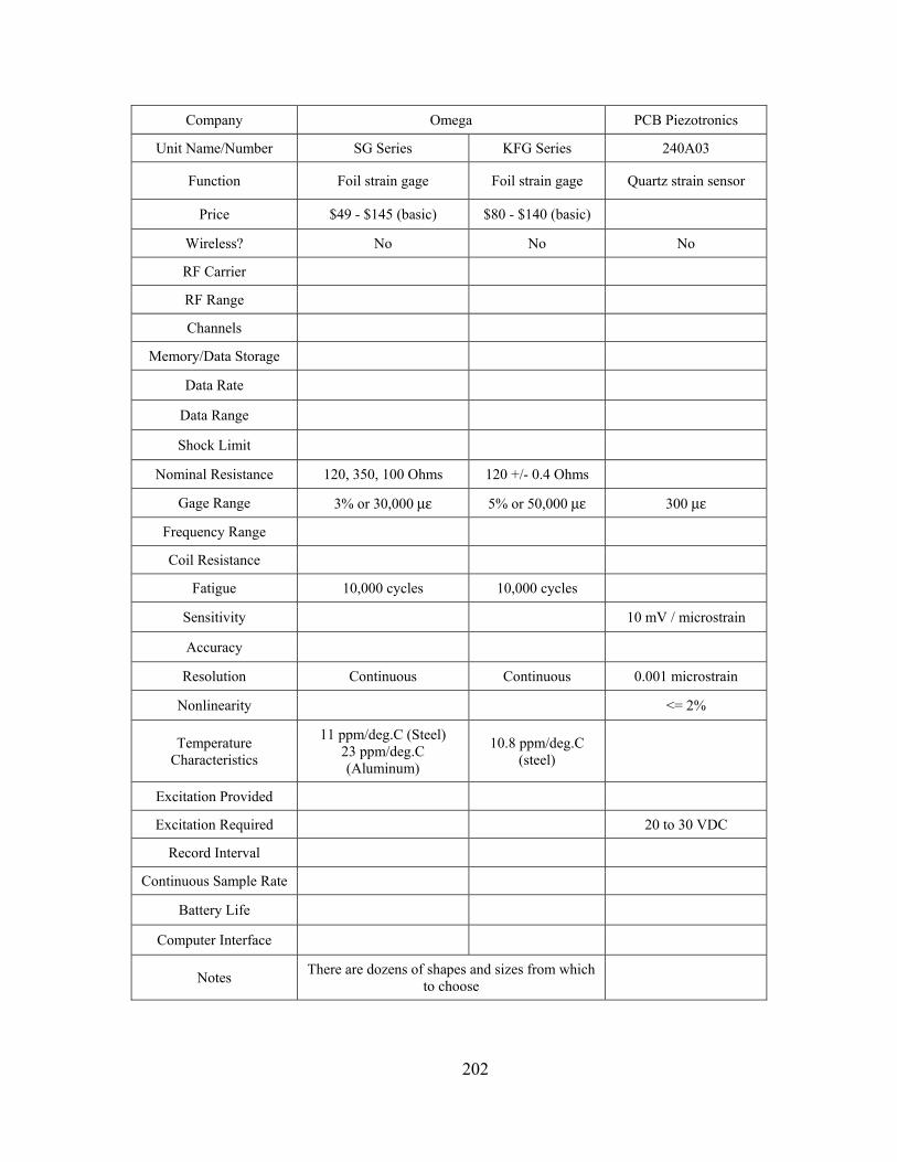
202
Company Omega PCB Piezotronics
Unit Name/Number SG Series KFG Series 240A03
Function Foil strain gage Foil strain gage Quartz strain sensor
Price $49 - $145 (basic) $80 - $140 (basic)
Wireless? No No No
RF Carrier
RF Range
Channels
Memory/Data Storage
Data Rate
Data Range
Shock Limit
Nominal Resistance 120, 350, 100 Ohms 120 +/- 0.4 Ohms
Gage Range 3% or 30,000 με 5% or 50,000 με 300 με
Frequency Range
Coil Resistance
Fatigue 10,000 cycles 10,000 cycles
Sensitivity 10 mV / microstrain
Accuracy
Resolution Continuous Continuous 0.001 microstrain
Nonlinearity <= 2%
Temperature Characteristics
11 ppm/deg.C (Steel) 23 ppm/deg.C (Aluminum)
10.8 ppm/deg.C (steel)
Excitation Provided
Excitation Required 20 to 30 VDC
Record Interval
Continuous Sample Rate
Battery Life
Computer Interface
Notes There are dozens of shapes and sizes from which to choose

203
A.2.3. TEMPERATURE
Company Analog Devices, Inc.
Model Name/Number AD- and TMP- Series AD- and TMP- Series
Function Analog IC transducer Digital IC transducer
Price $0.40 to $6.51 $0.59 to $2.95
Wireless? No No
Temp Range -55 to 150 deg. C (varies) -55 to 150 deg. C (varies)
Error +/- 0.5 to 2.5 deg. C +/- 0.5 to 3 deg. C
Resolution 1 micro-A per deg. K 5 to 28 mV per deg. C
10- to 16-bit 0.025 to 0.3 deg. C per LSB
Excitation Provided 2.7 to 30 V 2.65 to 7 V
A.2.4. TILT
Company Geokon
Unit Name/Number 6350
Function Vibrating wire
Wireless? No
Price
Data Range +/- 15 deg.
Sensitivity
Resolution 8 arc sec
Accuracty 0.10%
Linearity 1.50%
Thermal Zero Shift 0.01% per deg. C
Operating Frequency 1400 - 3500 Hz
Coil Resistance 180 Ohm
Notes

204
A.2.5. WIRELESS NETWORKING
Company Omega Summation Research
Unit Name/Number OM-CP-RFEXT-KIT ST-540 SR-540
Function RF Range Extender Data transmitter Data receiver
Price $599 per extender $999 per pair
$1,645 (1-channel) $2,395 (4-channel) $3,145 (8-channel)
$2,745
Frequency 900 MHz 915, 868, or 433 MHz 915, 868, or 433 MHz
Transmit Power 100 MW
Transmit Range 600 to 1500 ft
(indoor) 0.5 to 1 mi (outdoor)
500 ft
Number of Channels 1, 4, or 8 16
Sample Rate 9.5 or 17 ksps
Sample Resolution 12- or 18-bit
Accuracy 0.5% typical 0.1% possible
Analog Output 0-5, 0-10, +/-5, +/- 10 VDC
Digital Output 12-bit
Computer Interface RS-232C or serial RS-232
Data Rate 2.4 thru 57.6 kbs 115 kbs
Notes Remotely mount any
OM-CP Series datalogger

205
A.2.6. CORROSION
Company ACM
Unit Name/Number Gill AC Field Machine
Function Galvanostat Portable Galvanostat
Wireless? No No
Price $20,000
Channels 4 12
Max Power 600 V or 1000 A 12 V
Power Supply 110/230 VAC 50-60 Hz 110/230 VAC 50-60 Hz or 12 VDC
Noise <3 microvolts <4 microvolts
Potentiostat
Compliance Voltage +/- 15 V +/- 12 V
Sweep Range +/- 3 V +/- 3 V
Sweep Resolution 25 microvolts 25 microvolts
Frequency Response 30 kHz 30 kHz
Measurement Accuracy 21 Bit A/D 21 Bit
Measurement Resolution 1 microvolt 1 microvolt
Sweet Rate 200 mV/second 200 mV/second
Frequency Response Analyzer
Frequency Range 10 microHz to 30 kHz 10 microHz to 30 kHz
Sample Rate 1 MHz 1 MHz
ADC 12 Bit 12 Bit
Galvanostat Resolution 1 microvolt 1 microvolt
Notes For laboratory use For field use