A Foreign currency options pricing model and application for the Zimbabwean market
68
Here is to the crazy ones, the misfits, the rebels, the troublemakers, the round pegs in the square holes, the ones who see things differently, you can quote them, disagree with them, glorify them or vilify them, but the only one thing you can’t do is ignore them because they change things... they push the human race forward and while some may see them as the crazy ones, we see genius, because the ones who are crazy enough to think that they can change the world, are the ones who do. By Steve Jobs. i
Transcript of A Foreign currency options pricing model and application for the Zimbabwean market

Here is to the crazy ones, the misfits, the rebels, the troublemakers, theround pegs in the square holes, the ones who see things differently, you canquote them, disagree with them, glorify them or vilify them, but the onlyone thing you can’t do is ignore them because they change things... theypush the human race forward and while some may see them as the crazyones, we see genius, because the ones who are crazy enough to think thatthey can change the world, are the ones who do. By Steve Jobs.
i
Abstract
This study involves the developement of a foreign currency option pricing applica-
tion from the Heston model and the Garman-Kohlhagen model in Visual Basic and
Excel. The Garman-Kohlhagen model has been adopted as the standard model for
pricing foreign currency options as it is a modification of the famous, Black-Scholes
(1973). However, we outline the limitations of the Garman-Kohlhagen model and
propose a better foreign currency pricing model, the Heston model. In the Hes-
ton model, instead of holding the volatility of exchange rate constant, volatility is
assumed to be stochastic and is defined by a stochastic differential equation. The
success of the Heston model is based on the calibration of its parameters, in this
regard, we employ the inverse problem model to calibrate the Heston model using
Excel Solver. After having calibrated the model, we evaluate the performance of
the Heston model against that of the Garman-Kohlhagen model. Furthermore we
perform sensitivity analysis to ascert the effect of the Heston model parameters
on option prices and also if the Heston model is able to account for flactuations in
exchange rates.
ii

AcknowledgementsI would like to take this opportunity to thank the Department of Statistics and
Operations Research who gave me this rare opportunity not only to learn but a
platform for me to apply all that I had acquired both in and out of University.
My greatest gratitude goes to my project supervisor Mr. Edward Chiyaka for his
time, patience, advice and guidance. I would also like to thank Mr. Xolani Ndlovu
from Old Mutual Zimbabwe, Mr Kgopotso Mosako from the Reserve bank of South
Africa, for helping with the data for this project and for their input in this re-
search. To my friends Joanna Mhlanga, Chengetai Chitungo, Siyanai Zhou, Moth-
abisi Nare, Diana Gasa, Caroline Makoni and Ntokozo Ndlovu thank you for your
support and loyalty. Above all to my friend Constantine Chideme who gave me the
idea behind this project, thank you so much for the support, for listening to me and
helping me polish up my ideas. Finally I thank God, who is my source of strength
and believing His word in James 1 verse 17, “ Every desirable and beneficial gift
comes out of heaven. The gifts are rivers of lights cascading from the Father of
light. There is nothing deceitful in God, nothing two faced, nothing fickle!!!!”
iii
Contents
1 Introduction 11.1. Introduction . . . . . . . . . . . . . . . . . . . . . . . . . . . . . . . . . 11.2. Background . . . . . . . . . . . . . . . . . . . . . . . . . . . . . . . . . 2
1.2.1. Options . . . . . . . . . . . . . . . . . . . . . . . . . . . . . . . . 31.2.2. Uses of Derivatives Instruments . . . . . . . . . . . . . . . . . 51.2.3. Importance of a derivatives market . . . . . . . . . . . . . . . . 71.2.4. Foreign Currency Option Pricing Models Fundamentals . . . 8
1.3. Statement of the Problem . . . . . . . . . . . . . . . . . . . . . . . . . 81.4. Aim of Study . . . . . . . . . . . . . . . . . . . . . . . . . . . . . . . . . 81.5. Research Objectives . . . . . . . . . . . . . . . . . . . . . . . . . . . . . 91.6. Importance of Currency Options . . . . . . . . . . . . . . . . . . . . . 91.7. Scope of Study . . . . . . . . . . . . . . . . . . . . . . . . . . . . . . . . 91.8. Summary . . . . . . . . . . . . . . . . . . . . . . . . . . . . . . . . . . . 10
2 Literature Review 112.1. Introduction . . . . . . . . . . . . . . . . . . . . . . . . . . . . . . . . . 112.2. Foreign Currency Pricing Models . . . . . . . . . . . . . . . . . . . . . 12
2.2.1. The Garman-Kohlhagen Model . . . . . . . . . . . . . . . . . . 132.2.2. Other foreign currency pricing models . . . . . . . . . . . . . . 16
2.3. Summary . . . . . . . . . . . . . . . . . . . . . . . . . . . . . . . . . . . 23
3 Methodology 243.1. Introduction . . . . . . . . . . . . . . . . . . . . . . . . . . . . . . . . . 243.2. Stochastic Differential Equations (SDEs) . . . . . . . . . . . . . . . . 25
3.2.1. Geometric Brownian motion (GBM) . . . . . . . . . . . . . . . 263.2.2. Ornstein-Uhlenberk Process . . . . . . . . . . . . . . . . . . . . 273.2.3. Square-root Process . . . . . . . . . . . . . . . . . . . . . . . . 27
3.3. The Heston Model . . . . . . . . . . . . . . . . . . . . . . . . . . . . . . 283.3.1. Examination of the Heston model parameters . . . . . . . . . 293.3.2. Risk Neutralized approach to option pricing . . . . . . . . . . 303.3.3. Numerical Solution for the Heston Model . . . . . . . . . . . 30
3.4. Visual Basic and Excel in obtaining a closed form solution for theHeston model . . . . . . . . . . . . . . . . . . . . . . . . . . . . . . . . 32
3.5. Model Calibration . . . . . . . . . . . . . . . . . . . . . . . . . . . . . . 323.6. Comparison between the Heston Model and the Garman-Kohlhagen
model . . . . . . . . . . . . . . . . . . . . . . . . . . . . . . . . . . . . . 333.6.1. Model accuracy . . . . . . . . . . . . . . . . . . . . . . . . . . . 33
iv
3.6.2. Model Fairness . . . . . . . . . . . . . . . . . . . . . . . . . . . 333.7. Sensitivity Analysis of Heston model parameters . . . . . . . . . . . . 343.8. Option Pricing Application . . . . . . . . . . . . . . . . . . . . . . . . . 343.9. Summary . . . . . . . . . . . . . . . . . . . . . . . . . . . . . . . . . . . 35
4 Data Analysis, Simulations and Results 364.1. Introduction . . . . . . . . . . . . . . . . . . . . . . . . . . . . . . . . . 364.2. Data and data sources . . . . . . . . . . . . . . . . . . . . . . . . . . . 374.3. Heston Model Calibration Results . . . . . . . . . . . . . . . . . . . . 384.4. Comparison of the Heston model to the Garman Kohlhagen model . 39
4.4.1. Interpretation of the table . . . . . . . . . . . . . . . . . . . . . 404.5. Sensitivity analysis of Heston model parameters . . . . . . . . . . . . 41
4.5.1. Changes to the correlation parameter ρ . . . . . . . . . . . . . 424.5.2. Changes in the value of the Correlation coefficient . . . . . . . 424.5.3. Changes in the value of volatility of the volatility process . . . 444.5.4. Analysis of the Volatility graph . . . . . . . . . . . . . . . . . . 45
4.6. Option Pricing Application . . . . . . . . . . . . . . . . . . . . . . . . 474.7. Summary . . . . . . . . . . . . . . . . . . . . . . . . . . . . . . . . . . . 48
5 Conclusions and Recommendations 495.1. Introduction . . . . . . . . . . . . . . . . . . . . . . . . . . . . . . . . . 495.2. Conclusions and Recommendations from the study . . . . . . . . . . . 505.3. Conclusion . . . . . . . . . . . . . . . . . . . . . . . . . . . . . . . . . . 515.4. Visual basic Application code for the Garman Kohlhagen model . . . 585.5. Data used to calibrate the Heston Model . . . . . . . . . . . . . . . . . 605.6. Generalised Reduced Gradient Optimization Method . . . . . . . . . 61
v
List of Figures
1.1 Volatility of the rand against the US dollar . . . . . . . . . . . . . . . 3
3.1 Methodology framework . . . . . . . . . . . . . . . . . . . . . . . . . . 25
4.1 Differences in Option prices between the Garman Kohlhagen, Realmarket Option prices and the Heston model prices . . . . . . . . . . . 41
4.2 Graphical representation of the differences between the Heston Modeland Garman Kohlhagen model as a result of the correlation coeffi-cient ρ . . . . . . . . . . . . . . . . . . . . . . . . . . . . . . . . . . . . . 44
4.3 Graphical representation of the differences between the Heston Modeland Garman Kohlhagen model as a result of the variance of volatility 46
4.4 Application to price options . . . . . . . . . . . . . . . . . . . . . . . . 47
5.1 Heston model Excel VB code page 1 . . . . . . . . . . . . . . . . . . . 575.2 Heston model Excel VB code page 2 . . . . . . . . . . . . . . . . . . . 585.3 Heston model Excel VB code page 3 . . . . . . . . . . . . . . . . . . . 595.4 Excel VB code Garman Kohlhagen Model . . . . . . . . . . . . . . . . 595.5 Sample of data used in Calibrating the Heston Model . . . . . . . . . 60
vi
List of Tables
4.1 Calibration results . . . . . . . . . . . . . . . . . . . . . . . . . . . . . 384.2 A comparison between the Heston and the Garman Kohlhagen model 394.3 Calibration results when ρ is fixed at 0.5 and -0.5 . . . . . . . . . . . 424.4 Sample data of correletaion coefficient ρ sensitivity analysis . . . . . 434.5 Calibration results when σ is fixed at 0.1 and 0.2 . . . . . . . . . . . 454.6 Sample data of variance of volatility σ sensitivity analysis . . . . . . 46
vii
Chapter 1
Introduction
1.1. Introduction
Currency is the creation of a circulating medium of exchange based on a store of
value. It evolved from two basic innovations: the use of counters to assure that
shipments arrived with the same goods that were sent, and the use of silver ingots
to represent value; both of these developments had occurred by 2000BC. Foreign
exchange refers to money denominated in the currency of another nation. A foreign
exchange rate is therefore a price at which two currencies can be exchanged against
each other (Cross, 1998). The exchange rate, is a major determinant of a nations
economic health and hence the well-being of all the people residing in it. Central
banks play two roles in the foreign exchange market. They intervene in the market
by buying or selling foreign currencies, and they also may be in the market as
agents for other central banks.
Introduction 2
1.2. Background
Since the dollarization from 2008 to the present date, Zimbabwean companies have
had the privilege of using the US dollar. Due to easy access of this currency, local
companies can now easily trade with other firms in South Africa, Botswana, Asia
and other countries. In trading with other countries, companies face the risk of for-
eign exchange rates flactuations, which can result in the value of their investments
decreasing and them making losses in the process. Rodgers (2013) reveals that a
large number of Zimbabwean companies that are predominantly import-oriented
were losing value on their imports because they were allowing their South African
suppliers to give them prices in US dollars instead of South African Rand. Accord-
ing to him, Zimbabwean companies are essentially being cheated by their South
African suppliers when they get priced in US dollars because the South African
company will be buying a hedge on the value of the transaction. Zimbabwean
trading companies should not take it for granted that just because they have been
offered a price in US dollars it is the best deal. They should ask for a rand price
and then shop for a hedging product that will immunise them from exchange rate
movements.
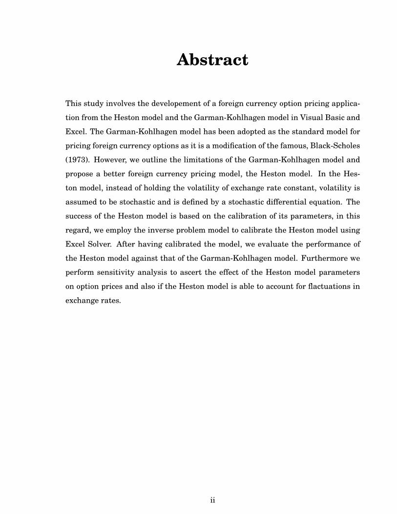
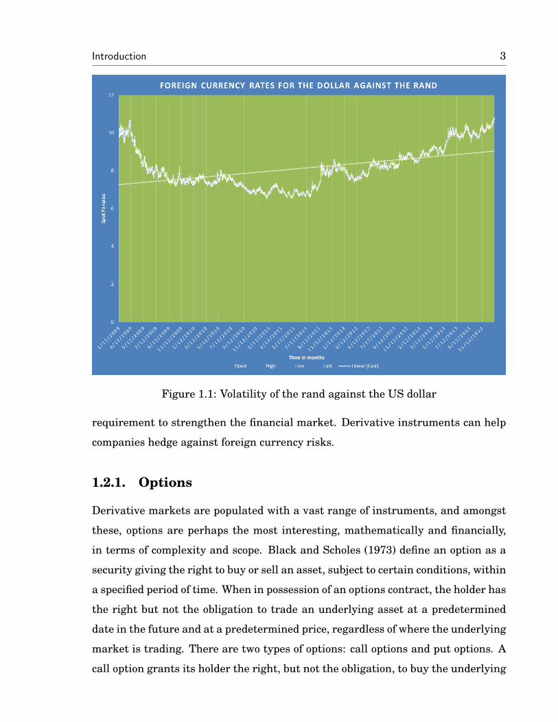
Recent observations on the US dollar and the Rand trading patterns reveal
that the rand has been very volatile against the US dollar since December 2009
to December 2013 as shown in Figure 1.1. The graph shows spot exchange rates
of the rand/US dollar against time and we observe that there has been a general
increase in the exchange rate between the rand and the dollar as shown by the
trend line. We also notice the frequent flactuations in exchange rate proving the
volatility of the rand against the dollar.
Although Zimbabwe is using a stable currency, the development of derivative
instruments has been very stunted and the community’s understanding of these
products is very shallow to a certain extent that the general traders don’t under-
stand these at all. According to Dodd, (2004) and Tian, (2005), derivatives are a
Introduction 3
Figure 1.1: Volatility of the rand against the US dollar
requirement to strengthen the financial market. Derivative instruments can help
companies hedge against foreign currency risks.
1.2.1. Options
Derivative markets are populated with a vast range of instruments, and amongst
these, options are perhaps the most interesting, mathematically and financially,
in terms of complexity and scope. Black and Scholes (1973) define an option as a
security giving the right to buy or sell an asset, subject to certain conditions, within
a specified period of time. When in possession of an options contract, the holder has
the right but not the obligation to trade an underlying asset at a predetermined
date in the future and at a predetermined price, regardless of where the underlying
market is trading. There are two types of options: call options and put options. A
call option grants its holder the right, but not the obligation, to buy the underlying
Introduction 4
asset(s) at a specified price on, and in some cases before, the date the option expires.
The specified price is called the strike price (or exercise price), the date the option
expires is called the maturity (or expiration date), and the premium (i.e. option
price) is the price paid to acquire the option. A put option is similar, but with the
right to sell the underlying asset(s).
Call and put options are further categorised in various ways based on their
additional features. These features include:
1. Underlying asset
Due to the enormous growth in financial markets, the use of options has be-
come increasingly popular and are available on many assets. Currently, op-
tions are actively traded on stocks, commodities, indices, foreign exchange
rates (of particular relevance to this study), futures, and even on weather
and electricity.
2. Exercise frequency
Options that can only be exercised at maturity are called European options
while those that can be exercised at any time up to maturity are called Amer-
ican options. Variants include Bermudan options, which can also be exercised
before maturity, but only on a fixed number of pre-determined dates during
the contract life.
3. Payoff functions
New types of options may be devised by changing the payoff function for the
option. For example, binary options have payoffs of either a fixed amount or
zero, rather than being linearly related to underlying asset value at maturity.
Whether the payoffs are achieved at all may be made to depend on the path
followed by the underlying asset. A barrier option, for instance, may cause
the payoff to be knocked out (alternatively, knocked in), dependent on path.
The payoffs from lookback options depend on the maximum or minimum as-
set price reached during their contract life. For Asian options, the payoffs
depends on the average price of the underlying asset during the life of the
contract.
Introduction 5
4. Moneyness (i.e. Intrinsic value)
This classification is mainly important in option price analysis. When the
strike price is equal to the spot price of the underlying asset, the option is
called an at-the-money option. When the strike price is greater than the spot
price of the underlying asset, the option is called an out-of-the-money call
option or an in-the-money put option. If the strike price is less than the spot
price of the underlying asset, the option is called an in-the-money call option
or an out-of-the-money put option.
Although regulated trading of options has not been done yet in Zimbabwe, regu-
lated options trading began in 1973 at the Chicago Board Options Exchange.
1.2.2. Uses of Derivatives Instruments
There are four main uses of derivative instruments which are Hedging, Specula-
tion, Arbitrage and Leverage (Chisholm, 2004). In his study, Chisholm outlined
the importance of derivative instruments through their application in asset man-
agement firms.
• Hedging refers to the action taken to protect an existing market position or
asset from an adverse market move for example a stock market crush that
could erode the value of a portfolio. The hedge is a position that would react
in an opposite manner, if the adverse market movement occurs. The idea will
be to offset the loss of value in the position being hedged. Chisholm (2004)
postulates that Asset Management Firms could hedge a share portfolio by
selling Futures that represent the portfolio held. He further asserts that not
only investing institutions like asset management firms, but also corpora-
tions, banks and governments can use derivative products to hedge or reduce
their exposures to market variables such as, share values, bond prices, cur-
rency exchange rates, interest rates and commodity prices.
• Hull (2001) defines speculation as entering a contract with the purpose of
making a profit. Portfolio managers in the form of speculators can take a fu-
ture position if they believe that they could make a profit. If they are bullish
Introduction 6
on the price of the underlying asset for example stock, they would buy the fu-
ture and then sell again once the price of the underlying asset had increased
sufficiently, making the future price rise. Similarly, if they feel that the un-
derlying asset is overpriced, they can sell the future and then buy back the
asset once the price has fallen. Chisholm (2004) asserts that derivatives in-
struments are very well suited to speculating on the prices of commodities
and financial assets and on key market variables such as interest rates, stock
market indices and currency exchange rates. It is much less expensive to
create a speculative position using derivatives than by actually trading the
underlying commodity or asset. As a result, the potential returns are that
much greater.
An arbitrage is a deal that produces risk free profits by exploiting a mispricing
in the market. A simple example occurs when a trader can purchase an asset
like Old Mutual shares which are dual listed both on ZSE and Johannesburg
Stock Exchange. The Old Mutual share is cheaper in one exchange and the
purchaser simultaneously arranges to sell it in another at a higher price.
Such opportunities are unlikely to persist for very long, since arbitrageurs
would rush in to buy the asset in the ‘cheap location, thus closing the pricing
gap.
• Leverage enables a greater gain (loss) to be made for a given amount of initial
capital employed-higher risk for higher returns. In this sense, derivatives
can be used as an efficient avenue to obtain leverage in financial markets.
For example, if a speculator in the form of asset mangers thinks a stock will
rise, they can purchase a call option on the stock. They use less capital than
buying the stock outright, since less money is required on the initiation of the
contract. In the case of the forward contract no money changes hands, while
with the option only the premium is paid. The leverage that can be acquired
in derivatives markets is also a highly attractive feature to those looking to
hedge, as it allows a smaller amount of money to be put up front in order to
Introduction 7
gain protection against changes in the asset price.
1.2.3. Importance of a derivatives market
Effenberger (2004) asserts that the volatility of financial markets can affect a firm,
thus managers should seek to avoid it. Initially many asset management firms
tried to build better forecasting models so that if they could predict price changes,
they could avoid the risk. Hamilton (1998) postulated that derivatives can be used
to combat the adverse effects of volatile commodity prices on the economies of de-
veloping countries because forward prices tend to be less volatile than spot prices,
giving commodity producers an opportunity to reduce the volatility of the price of
their output through hedging.
The Deustche Bundesbank report (2006) states that an active derivatives ex-
change plays an important role in facilitating an efficient determination of prices
in the underlying cash (or spot) market by providing improved and transparent
information on both current and future prices for an asset. For example, in com-
modity markets, spot prices are often pegged to futures prices because the futures
market provides excellent pricing information for the underlying product. Prices on
derivatives markets reflect anticipated supply and demand, and derivatives mar-
kets thus enhance the ability of market participants to make decisions about future
production processing, and trade.
Derivatives can be used to generate and deliver abnormal performance that can
be packaged within a core-satellite approach to portfolio management, that option
portfolios can be used to enhance the performance of tactical asset allocation pro-
grammes and that fixed-income derivatives offer significant risk reduction benefits.
Introduction 8
1.2.4. Foreign Currency Option Pricing Models Fundamen-
tals
The development of Nobel-prize winning Black Scholes (1973) model on pricing an
option rejuvenated modern quantitative finance in the early 1970s. Based on the
Black Scholes Model, a standard approach to pricing foreign currency options was
developed by Garman-Kohlhagen (1983). This approach took into consideration
six fundamental variables in determining the price of an option on an exchange
rate. These variables include: the current (spot) price, the strike price, the time
to expiration, the foreign currency interest rate, the domestic currency interest
rate, and volatility. Most models that have been developed to price options, seek to
quantify the magnitude in which these individual variables affect the price of an
option. For instance, on volatility, the Garman Kohlhagen model assumes volatility
to be constant, whereas Melino and Turnbull (1990) considered the existence of
stochastic volatility.
1.3. Statement of the Problem
This study seeks to develop a foreign currency options pricing model that can be
used by various players (investment banks, brokers, arbitrageurs) in the Zimbab-
wean financial markets. There is need for a foreign exchange options market where
Zimbabwean companies and individual traders can hedge themselves against for-
eign currency risks. These instruments have not been traded in Zimbabwe, hence
this study will be based on the assumption that a trading system similar to the one
used on the Johannesburg Stock Exchange (JSE) will be used by the Zimbabwe
Stock Exchange (ZSE) in trading these instruments.
1.4. Aim of Study
This study seeks to develop an application for pricing foreign currency options.
Introduction 9
1.5. Research Objectives
The main objectives of this study are as follows:
• Analyse the effect of stochastic volatility on foreign currency options with
particular interest being on the significant difference between the Heston and
the Black Scholes (Garman Kohlhagen, 1983) model.
• Modify and calibrate the Heston model, to make it a better suited foreign
currency option pricing model for the Zimbabwean market.
• To develop a user friendly foreign currency option pricing application that can
be used in Over the Counter markets.
1.6. Importance of Currency Options
Currency options are widely used to hedge foreign exchange risk for a future date.
They provide foreign exchange risk managers, investors and traders with a wide
array of capabilities for controlling the risks inherent in foreign exchange exposure,
and for participating in market movements and implementing investment research
decisions related to exchange rate flactuations. In academic research, currency
options are important in measuring the value of other international financial in-
struments, such as currency option bonds, currency future options, currency option
forwards and so on. As international financial markets further develop, currency
options will play an increasingly important role as a major international financial
instrument.
1.7. Scope of Study
This project will encampass studies on Foreign currency option pricing. A num-
ber of models have been developed in the past to price foreign currency options,
these include the Garman Kohlhagen (1983) model, stochastic volatility models
and jump diffusion option pricing models. In this study we focus on the Garman
Introduction 10
Kohlhagen model and stochastic volatility models with particular interest being on
the Heston model for Stochastic volatility models. When determining a closed form
solution for the Heston model, a number of variables are used. To estimate the
exact value of these variables, optimisation techniques are applied. This is called
calibration of the Heston model. To calibrate the Heston model we use the inverse
method from a number of methods which will be highlighted in the chapter 3. The
inverse problem can be solved by a number of optimisation tools like Matlab, Lingo
and Microsoft excel. In this study we use Microsoft excel as it is very user friendly,
accessible, easy to understand and produces fairly accurate results.
Furthermore through this study, the researcher develops an application that
seeks to determine the premium value of an option. This application should allow
the user to choose a pricing model they want to use in determining the option price.
Among the models to be chosen from will be the Garman Kohlhagen model and the
Heston model.
The main African countries that Zimbabwe trades with are Botswana and South
Africa of which the later has got a higher trade ratio than the former. In this regard
this study will focus on the following currency pairs:
• USD/ZAR,
• USD/GBP, and
• USD/BWP.
1.8. Summary
This chapter gives a basic overview of foreign currency derivatives. The researcher
highlights the basic need for foreign currency derivatives in Zimbabwe, further-
more the researcher seeks to unravel what foreign currency options are, the struc-
ture and role of the foreign exchange market and finally the fundamentals of for-
eign currency options pricing.
Chapter 2
Literature Review
2.1. Introduction
In this chapter, we consider aspects surrounding foreign currency options pricing.
According to Chensey and Scott (1989), when developing an option pricing model,
financial engineers seek to achieve two objectives:
1. Deteremine a fair price for an option, and
2. Develop an accurate model comparing model values to observed values.
Various models have been developed to price options, the famous of them all being
the Nobel Prize winning Black Scholes model 1973. The Black Scholes model laid
a foundation to stock option pricing and has been widely used in over the counter
markets and organised exchanges to determine the fair prices of a stock option.
The main advantages of the Black Scholes model that have ensured its continuous
recognition in the financial markets is that it is fast and easy to use. By providing
a way of calculating hedge ratios and more efficient portfolios, the Black Scholes
model also helps investors understand the sensitivity of option prizes to stock price
movements, thereby helping investors maximize the efficiency of their portfolios.
Literature Review 12
Finally the Black Scholes steadies the market because of its ability to measure
equilibrium pricing relationships.
However inspite of its successes and advantages, Rubinstein (1985) asserts that
the Black Scholes model has known biases. These biases include:
1. Constant volatility assumption
The Black Scholes model assumes constant volatility of stock prices, of which
this assumption is strongly violated in financial markets. In financial mar-
kets, volatility tends to exhibit consistently the following traits:
• Volatility tends to revert around some long term value.
• Volatility clusters with time: large (small) changes tend to follow large
(small) price changes.
• Volatility is correlated to stock return.
2. The leverage effect
The Black Scholes model can not account for the leverage effect which is but
just the tendency for stock prices to be negatively correlated with changes in
volaltility.
Meisner and Labuszewski (1984) illustrate how the Black Scholes model can be
modified to tailor make it for the pricing of various assets options, for example, the
Garman-Kohlhagen model (1983) modified the Black Scholes model to price foreign
currency options.
2.2. Foreign Currency Pricing Models
Jarrow (1991), defines a European foreign currency call (put) option as a derivative
instrument that gives the holder the right to buy (sell) a fixed amount of the foreign
currency or currency futures, respectively, at a predetermined price only at the
fixed expiration date. The corresponding American options can be exercised at any
time until the expiration date.
Currency options pricing models are dependant mainly on the following factors:
Literature Review 13
• Exchange rate,
• Interest rate, and
• Anticipated volatility of the exchange and interest rates.
We review literature on models that have been developed to pricing foreign cur-
rency options. Much attention is given to the Garman-Kohlhagen model (1983)
which is a direct modification of the Black-Scholes model and has been widely used
in foreign currency options pricing across counters.
2.2.1. The Garman-Kohlhagen Model
According to Garman-Kohlhagen (1983) a model for pricing foreign currency op-
tions can be developed from the Black-Scholes formula. This model is based on the
following assumptions:
1. No transaction costs, no differential taxes, no borrowing or lending restric-
tions, and trading takes place continuously.
2. The term-structure of interest rates in both the domestic and foreign country
are flat and non-stochastic.
3. The underlying state variable is the spot exchange rate
4. The exchange rate S can be described by the stochastic process
dS = BSdt+ σSdZ, (2.1)
where B is the instantaneous mean, σ2 is the instantaneous variance; and Z
is a standard Wiener process. It is also assumed that B and σ are constants,
implying that the stochastic process describing the evolution of the spot rate
over time is log-normal.
Literature Review 14
Given the above assumptions and further referring to Merton (1973), Garman
and Kohlhagen (1983) value an European option by the following formula:
C = exp(−rFT )SN(d1)− exp(−rDT )KN(d2), and (2.2)
P = −exp(−rFT )SN(−d1) + exp(−rDT )KN(−d2), (2.3)
where:
• C is the Call option price and P is the Put option price.
• rD (rF ) is the domestic (foreign) risk free interest rate per unit time.
• T is the maturity of the option: T ≡ T1 − t where T1 is the date the option
matures and t the current time.
• K is the exercise price.
• d1 ≡ ln(S/K)+((rD−rF )+σ2/2)Tσ√
T.
• d2 ≡ d1 − σ√T .
• N(.) is the cumulative normal distribution function.
Drawbacks of the Garman-Kohlhagen Model
Underlying the Garman-Kohlhagen options valuation formula are a number of as-
sumptions. To the extent that the world deviates from these assumptions, the
Garman-Kohlhagen model will be biased in certain, often predictable ways. This
subsection explores the pricing biases introduced by two major simplifying assump-
tions of the Garman-Kohlhagen model: constant volatility and a normal (or lognor-
mal) distribution of price changes. The Garman-Kohlhagen may not be a perfect
model of options valuation, but as long as market participants understand these
and other problems with the model, then it is useful in practice.
The Garman-Kohlhagen model assumes that an exchange rate’s volatility is
known and never changes. However, causal observation reveals exchange rate
Literature Review 15
volatility is not constant. This fact has a major impact on the values of certain
options, especially those options that are away from the money, because the dy-
namics of the volatility process rapidly change the probability that a given out
of the money option can reach the exercise price. The Garman-Kohlhagen model
consistently underestimates the value of an option to the extent that volatility is
stochastic rather than constant as assumed.
A second major assumption of the Garman-Kohlhagen model is that exchange
rate returns are normally (or lognormally) distributed with a variance proportional
to the length of time over which the asset trades. However, a number of academic
studies show that exchange rate movements are neither normally nor lognormally
distributed. Empirically, exchange rates experience big moves with a frequency
that exceeds what one would expect theoretically. This could be a result of herd
like behaviour among currency speculators or it could be due to the intervention of
central banks. Once again, this problem with the distributional assumption of the
Black-Scholes model means that it generally underestimates currency option val-
ues because the likelihood of having an extreme price movement is greater than the
model expects. As with the Black-Scholes (1973) model, the Garman-Kohlhagen
formula has been a popular practical choice for currency option pricing over the
years, despite the fact that interest rate and volatility are not constant in practice.
Biger and Hull (1983) again used the Black-Scholes (1973) methodology includ-
ing dividends, and obtained comparable results based on the same assumptions
as employed by Garman and Kohlhagen (1983). In the same year, Grabbe (1983)
presented a model for European options, which relaxes the assumption of constant
interest rates. He assumed that the processes of interest rates in the domestic
currency and the foreign currency are deterministic functions of time, using an
arbitrage-free approach to obtain a partial differential equation (PDE) and con-
sequently the European call price. However, the model is not supported by the
empirical evidence of Adams and Wyatt (1987a), who showed that the interest rate
risk is an important element in the valuation of currency options.
Literature Review 16
2.2.2. Other foreign currency pricing models
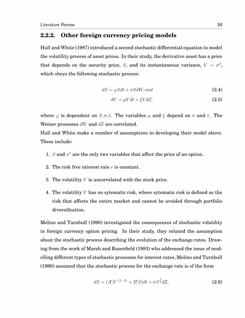
Hull and White (1987) introduced a second stochastic differential equation to model
the volatility process of asset prices. In their study, the derivative asset has a price
that depends on the security price, S, and its instantaneous variance, V = σ2,
which obeys the following stochastic process:
dS = ϕSdt+ σSdW, and (2.4)
dV = µV dt+ ξV dZ, (2.5)
where ϕ is dependent on S, σ, t. The variables µ and ξ depend on σ and t. The
Weiner processes dW and dZ are correlated.
Hull and White make a number of assumptions in developing their model above.
These include:
1. S and σ2 are the only two variables that affect the price of an option.
2. The risk free interest rate r is constant.
3. The volatility V is uncorrelated with the stock price.
4. The volatility V has no sytematic risk, where sytematic risk is defined as the
risk that affects the entire market and cannot be avoided through portfolio
diversification.
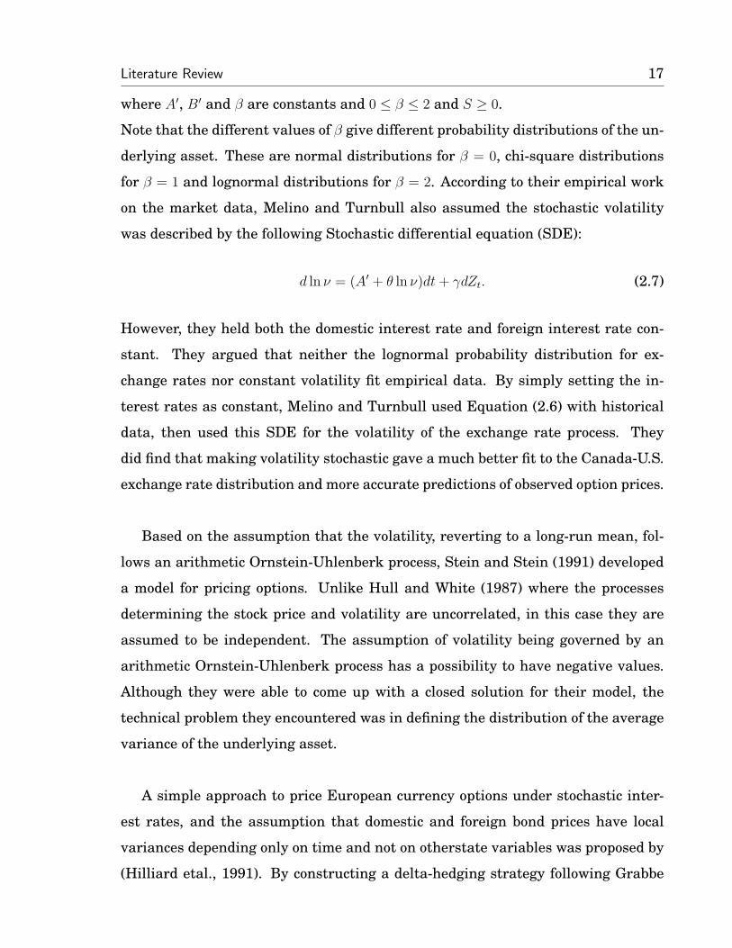
Melino and Turnbull (1990) investigated the consequences of stochastic volatility
in foreign currency option pricing. In their study, they relaxed the assumption
about the stochastic process describing the evolution of the exchange rates. Draw-
ing from the work of Marsh and Rosenfield (1983) who addressed the issue of mod-
elling different types of stochastic processes for interest rates, Melino and Turnbull
(1990) assumed that the stochastic process for the exchange rate is of the form
dS = (A′S−(1−β) +B′S)dt+ σSβ2 dZ, (2.6)
Literature Review 17
where A′, B′ and β are constants and 0 ≤ β ≤ 2 and S ≥ 0.
Note that the different values of β give different probability distributions of the un-
derlying asset. These are normal distributions for β = 0, chi-square distributions
for β = 1 and lognormal distributions for β = 2. According to their empirical work
on the market data, Melino and Turnbull also assumed the stochastic volatility
was described by the following Stochastic differential equation (SDE):
d ln ν = (A′ + θ ln ν)dt+ γdZt. (2.7)
However, they held both the domestic interest rate and foreign interest rate con-
stant. They argued that neither the lognormal probability distribution for ex-
change rates nor constant volatility fit empirical data. By simply setting the in-
terest rates as constant, Melino and Turnbull used Equation (2.6) with historical
data, then used this SDE for the volatility of the exchange rate process. They
did find that making volatility stochastic gave a much better fit to the Canada-U.S.
exchange rate distribution and more accurate predictions of observed option prices.
Based on the assumption that the volatility, reverting to a long-run mean, fol-
lows an arithmetic Ornstein-Uhlenberk process, Stein and Stein (1991) developed
a model for pricing options. Unlike Hull and White (1987) where the processes
determining the stock price and volatility are uncorrelated, in this case they are
assumed to be independent. The assumption of volatility being governed by an
arithmetic Ornstein-Uhlenberk process has a possibility to have negative values.
Although they were able to come up with a closed solution for their model, the
technical problem they encountered was in defining the distribution of the average
variance of the underlying asset.
A simple approach to price European currency options under stochastic inter-
est rates, and the assumption that domestic and foreign bond prices have local
variances depending only on time and not on otherstate variables was proposed by
(Hilliard etal., 1991). By constructing a delta-hedging strategy following Grabbe
Literature Review 18
(1983), invoking the risk-neutrality argument of Cox and Ross (1976), and by
identifying Vasicek’s (1977) term structure model as the appropriate bond pric-
ing model, (Hilliard etal., 1991) derived a closed-form European currency-option
pricing model under stochastic interest rates. Unfortunately, the Vasicek model al-
lows the occurrence of negative interest rates, which is unreasonable,and moreover,
these models cannot be extended to American option pricing analytically. (Hilliard
etal., 1991) model is competitive for currencies with highly volatile interest rates
and for long-lived options. (Hilliard etal., 1991), and Amin and Bodurtha (1995)
indicated that allowing for stochastic interest rates leads to a more accurate val-
uation of currency options with longer maturities than the constant interest rates
alternative.
Tucker (1991) suggested that foreign exchange rates follow a jump-diffusion
process, and that an option pricing model, that takes this process into account, is
likely to be more accurate. Many other authors also demonstrate that these large
jumps exist in foreign exchange price movements, which are responsible for the
leptokurtic distribution on price returns (i.e. the inflation of peak and tails as the
result of the occurrence of more frequent small and large price changes than nor-
mal). Unfortunately, Tucker also assumes that interest rates are non-stochastic.
A general framework for valuing a European option on a foreign currency with
stochastic interest rates was introduced by Amin and Jarrow (1991). Their model
allowed domestic and foreign term structures of interest rates to follow the stochas-
tic processes of the (Heath etal., 1992) (hereafter, HJM) structure. Amin and Jar-
row (1991) also obtained closed-form solutions for European options by assuming
the market is complete and the volatility functions governing the term structure
are deterministic. The Amin and Jarrow (1991) model is a multi-factor model in
which there are at least three different sources of uncertainty, those associated
with the domestic interest rate, the foreign interest rate, and the exchange rate.
To find a risk-free equivalent martingale measure, they chose the domestic current
account (i.e. the cash account) as the numeraire and calibrated the domestic bond,
Literature Review 19
the foreign bond and the exchange rate into the new equivalent martingale mea-
sure, and obtained an analytic solution for European-style options. However, the
complexity of the assumptions of the Amin and Jarrow model make it applicable
only to European-type options. Even using numerical approaches, it is diffcult to
implement the HJM framework.
The first highly stochastic currency-option model allowing American-style (i.e.
early exercise) feature was produced by Amin and Bodurtha (1995). In their model
they considered an arbitrage-free discrete time implementation of the Amin and
Jarrow (1991) framework, using a multinomial version of the lattice technique of
(Cox etal., 1979). They derived a path-dependent model with specific interest-rate
functions. A property of path dependence is that the outcome of a process depends
on its past history, which implies the tree cannot recombine. Therefore it is diffi-
cult to obtain an accurate result due to the vast computational cost. In Amin and
Bodurtha’s model, a simplified HJM model is adopted. They assumed the volatil-
ities of both the domestic and the foreign forward rates are constant (i.e. the Ho
and Lee, 1986 model). Moreover, they only managed to obtain up to 12 time steps
for a five-year American put option value. The multinomial tree with only 12 time
steps applied to a three-factor model is rather unsatisfactory, although it is stated
in their paper:
“... for option maturities up to five years, path-dependent models with
fewer than 12 steps can still yield option values that are accurate to
within one or two percent of their continuous-time limiting values.”
Since there is no benchmark for the American option price with stochastic interest
rates, they adopted a path-independent model in their paper, with a recombining
tree. However, the accuracy of the recombine tree is rather poor, there remains
much scope for improvement in early-exercise currency option pricing which sub-
sequent work has not adequately addressed.
Literature Review 20
Bakshi, Cao and Chen (1997) stated that many assumptions can be made con-
cerning the distribution of the underlying asset, the interest rates components and
the market price of risk. They used a generalised least-squares technique to esti-
mate the parameters, essentially minimising an error term each day of the sample.
This approach, although straight forward to implement, is somewhat contrary to
the assumptions of the model, as it allows the parameters to take on a different
value every day. Moreover, obtaining parameters using cross-sectional information
may result in an excellent fit at the current date, but does not provide any infor-
mation about the dynamics of the system.
Chang (2001) extended Geske and Johnson’s (1984) approach to a stochastic
interest-rate economy. He used only the values of once and twice exercisable op-
tions and described how stochastic interest rates affect the option value. He built a
tree of forward exchange rate process StBf
Bdwhere St was the spot exchange rate at
time t, Bf was a foreign bond and Bd was a domestic bond. However, Chang’s paper
suffers the disadvantage of tree methods, as mentioned for Amin and Bodurtha’s
(1995) model, which is computationally inefficient and is difficult to apply to Amer-
ican options.
A numerical improvement to Amin and Bodurtha’s (1995) model was made by
Choi and Marcozzi (2001). They used a radial basis function (RBF) methodology
to approximate the PDE for currency options. Choi and Marcozzi transformed the
HJM framework into a short-rate version to obtain a Partial differential equation
and established a risk-neutral measure by using the domestic interest rate as a
risk-free numeraire. However, they presented numerical results for a one-year
option with merely five steps for both the foreign interest rate and the domestic
interest rate processes, 31 steps for the exchange rate and 360 time steps for a
one-year option.
Choi and Marcozzi (2003) managed to obtain an analytic solution for European
currency-options. They considered the state variables to be the short rates of in-
Literature Review 21
terest and the exchange rate, as opposed to the forward rates as proposed in Amin
and Jarrow (1991) and utilised in Amin and Bodurtha (1995), in which case the as-
sociative diffusion representing the global economy possesses a coercive diffusion
matrix.
A model that focused on the exchange-rate process with jump diffusion was
proposed by Chesney and Jeanblanc (2004). In their model they obtained a Par-
tial differential equation for a European option, then claimed, “If the American
and European option values satisfied the same linear PDE (in the continuation re-
gion), their difference ∆C, the American premium, must also satisfy this Partial
differential equation in the same region.” Unfortunately, the sign of the jump size
significantly affects the pricing model. Only negative-jump processes can be priced
and furthermore, Partial differential equations describing American options are
inherently nonlinear and, as a consequence, the quantity ∆C cannot satisfy the
same Partial differential equation.
A two dimensional random diffussion proces to model the dynamics of an as-
set price is exploited by Parello, etal (2008). They assume that the stock price
is governed by a log-Brownian motion and that the Ornstein Uhlernberk process
describes the randomness of the log-volatilty and that the two Weinner processes
are correlated. Although the derivation process of a closed form solution to their
model is tedious and laborious, after making a number of assumptions and using
the Fokker-Planck Equation, they come up with a closed form solution. The key
in obtaining an accurate pricing model through their approach is in calibrating for
the parameters that were used in the derivation process.
Dupoyet (2006) undertook an empirical investigation into Japanese Yen/U.S.
Dollar currency-options traded on the Philadelphia stock exchange during March
29th, 1996 to December 31st, 1999, with the aim of determining the information
content of European option prices (for which analytic solutions are available). The
models tested were Black-Scholes (1973) and three others, using stochastic volatil-
Literature Review 22
ity, stochastic interest rates and stochastic volatility with jumps. In order to in-
crease the sample size, both European calls and American calls were studied, in
a stochastic interest-rate environment where American call values could be safely
approximated by corresponding European call values (with the Japanese interest
rate much lower than U.S. interest rate). The greatest improvement over Black-
Scholes in pricing and hedging was found by using stochastic volatility. Stochastic
interest rates improved pricing only for in-the-money long-term options, with in-
significant effect on hedging; including jumps improved pricing and the volatility
smile, but again contributed little to hedging.
Although there is a wide concensus that volatility plays a key role in the dy-
namics of financial markets, there still seem to be no acceptable model which can
realy predict volatility as it is unobservable.
In this study we will use the Heston model (1993). Heston (1993) pioneered the
developement of stochastic volatility in currency option models. As volatility is an
unobservable yet very important parameter, Heston applied a mean-reverting fea-
ture to the volatility process. Thus the model is composed of a stochastic domestic
zero-coupon bond, a foreign zero-coupon bond, an exchange rate, and the volatility
of the exchange rate process. Heston obtained a partial differential equation by
delta-hedging two different maturity portfolios in the model, and then obtained an
analytic solution by invoking the Black-Scholes (1973) formula. Although Heston’s
model has been influential, he assumed interest rates are non-stochastic, which
is somewhat inconsistent with the stochastic bond prices in the model. Also it
is heuristic since he separated Garman-Kohlhagen’s formula into two probability
parts and assumed these satisfy the partial differential equation independently in
order to obtain the option price. Despite its limitations stated above we use the
Heston (1993) model because it has the following advantages:
• It provides a closed-form solution for a European call option.
• It is able to explain the property of stock price when its distribution is non-
Literature Review 23
Gaussian.
• It fits the implied volatility surface of the option prices in the market.
• It allows the correlation between stock price and volatility to be negative.
The number of option pricing models that can be derived is virtually unlimited
because of the many combinations of assumptions that are possible. A number of
models have attempted to capture many processes simultaneously (see Nawalkha
and Chambers, 1995). Such models include the stochastic volatility and stochastic
interest rate models of Amin and Ng (1993), Bakshi and Chen (1997), the stochastic
volatility and jump models of Bates (1996), and the stochastic interest rates and
jump-diffusion models of Doffou and Hilliard (2001).
2.3. Summary
Throughout this chapter, we reviewed literature on foreign currency option pricing.
An overview of the standard Black-Scholes model (1973) was done,thereafter we
reviewed the Garman-Kohlhagen model (1983) which is a direct evolution of the
Black-Scholes model (1973). Although successful in pricing foreign currency op-
tions, the Garman-Kohlhagen model (1983) assumes constant volatility of interest
and exchange rates, and this has resulted in other researchers developing stochas-
tic volatility models so as to account for flactuations in volatility. The researcher
thereby reviewed literature on stochastic volatility models and finally settles on
the Heston model which will be used in pricing foreign currency options in this
research project. The success and significance of the Heston model is based on the
calibration for its input parameters, in the next chapter, methodology, a great deal
of effort will be made to establish a better suited method for calibrating the Heston
model.
Chapter 3
Methodology
3.1. Introduction
In this study, the Heston model (1993) is applied to determine the price of a foreign
currency option. Past studies that have been conducted on option pricing stand to
prove that the Garman-Kohlhagen model (1983) has got a lot of biases as a result
of the assumptions on which it is built upon. One of these assumptions is that
it assumes constant volatility of exchange rates, this assumption results in the
Garman-Kohlhagen model not meeting the common phenomenon in option pricing
which is the volatility smile.
After having applied the Heston model to price an option, we then compare its
performance to the Garman-Kohlhagen model. Two main foundations of option
pricing are used as a basis for comparison, and these include the fairness of the op-
tion price and the accuracy of the model as compared to real market values. There
are a number of steps that are taken in doing so, and this process involves the use
of Visual basic and Optimisation models to calibrate the Heston model. Once this
process is done a user friendly application that allows the user to price a foreign
Methodology 25
currency option is developed. This application will be able to determine the option
price for the ZAR/USD, BWP/USD, GBP/USD and finally the Euro/USD currency
pairs. Various counters have different risk appetites. In this regard, both the He-
ston model and the Garman-Kohlhagen model will be used as the main models in
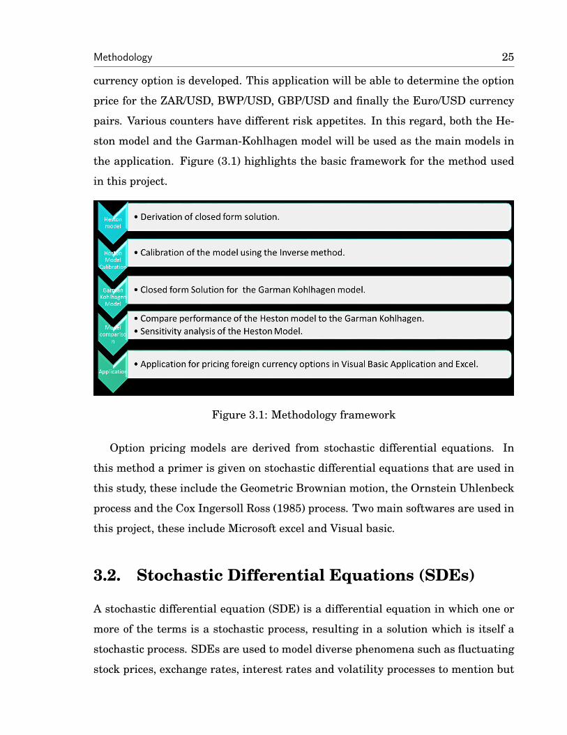
the application. Figure (3.1) highlights the basic framework for the method used
in this project.
Figure 3.1: Methodology framework
Option pricing models are derived from stochastic differential equations. In
this method a primer is given on stochastic differential equations that are used in
this study, these include the Geometric Brownian motion, the Ornstein Uhlenbeck
process and the Cox Ingersoll Ross (1985) process. Two main softwares are used in
this project, these include Microsoft excel and Visual basic.
3.2. Stochastic Differential Equations (SDEs)
A stochastic differential equation (SDE) is a differential equation in which one or
more of the terms is a stochastic process, resulting in a solution which is itself a
stochastic process. SDEs are used to model diverse phenomena such as fluctuating
stock prices, exchange rates, interest rates and volatility processes to mention but
Methodology 26
a few.
The theory of stochastic differential equations is a framework for expressing
dynamical models that include both random and deterministic components; the
theory being based on the Ito integral. The solution to an SDE is a stochastic pro-
cess which is expressed in terms of a stochastic integral with respect to Brownian
motion. Stochastic differential equations form the basis of option pricing. In this
study we use stochastic differential equations to:
1. Determine the foreign currency option price, and to
2. Model volatility of exchange rates.
3.2.1. Geometric Brownian motion (GBM)
A Geometric Brownian motion is the most common process utilised in financial
market modelling, and can be used to model the uncertain return of an asset, such
as a stock. The SDE of a Geometric Brownian motion is defined as
dXt
Xt
= µdt+ σdBt, (3.1)
with initial values X0 = x0 where µ ∈ < and σ ≥ 0.
In this model, σ is the volatility and µ is the mean return. Bt is the Weiner process
and Xt is the asset price
The solution to the GBM is:
Xt = X0eµ−σ2
2t + σBt. (3.2)
It is clear that Xt has a normal distribution with expectation and variance condi-
tioned on X0 = x0 given by
E[Xt|x0] = x0eµt, and (3.3)
V ar[Xt|x0] = x20e
2µt(1− eσ2t). (3.4)
Methodology 27
respectively. Equation (3.1) is used to model the exchange rate process for the
Garman-Kohlhagen model because it has a desirable memoryless property, i.e, to
make a prediction of the value of X at time t we only need to know the value of X
now, not anything about the path it took to get to the present value.
3.2.2. Ornstein-Uhlenberk Process
A stochastic process is called an Ornstein-Uhlenberk process if the SDE has the
form
dXt = κ(θ −Xt)dt+ σdBt, (3.5)
where κ is the rate of mean reversion, θ is the long term mean of asset price and
σ is the volatility, and Bt is a Weiner process with the initial value X0 = x0. The
solution to the Ornstein-Uhlenberk process is
Xt = θ + (x0 − θ)e−κt + σ
∫e−θ(t−s))dBs. (3.6)
Note that Xt has a normal distribution with the expectation and variance, condi-
tioned on X0 = x0 given by
E[Xt|x0] = θ + (x0 − θ)e−κt, and (3.7)
V ar[Xt|x0] =σ2
2κ(1− e−2κt). (3.8)
In finance, the Ornstein Uhlenberk process is a widely used for the term structure
model of interest rates, including the Vasicek (1977) model because its drift com-
ponent is not constant as in the GBM but is dependant on the current value of the
process Xt, if the current value is less than the long term mean θ, then the drift will
be positive, if it is greater than the long term mean, then the drift will be negative.
3.2.3. Square-root Process
A process
dXt = κ(θ −Xt)dt+ σ√XtdBt (3.9)
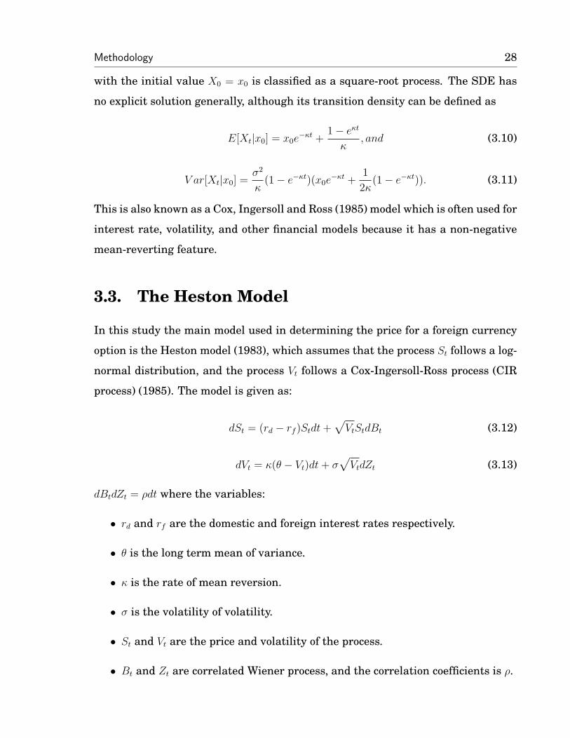
Methodology 28
with the initial value X0 = x0 is classified as a square-root process. The SDE has
no explicit solution generally, although its transition density can be defined as
E[Xt|x0] = x0e−κt +
1− eκt
κ, and (3.10)
V ar[Xt|x0] =σ2
κ(1− e−κt)(x0e
−κt +1
2κ(1− e−κt)). (3.11)
This is also known as a Cox, Ingersoll and Ross (1985) model which is often used for
interest rate, volatility, and other financial models because it has a non-negative
mean-reverting feature.
3.3. The Heston Model
In this study the main model used in determining the price for a foreign currency
option is the Heston model (1983), which assumes that the process St follows a log-
normal distribution, and the process Vt follows a Cox-Ingersoll-Ross process (CIR
process) (1985). The model is given as:
dSt = (rd − rf )Stdt+√VtStdBt (3.12)
dVt = κ(θ − Vt)dt+ σ√VtdZt (3.13)
dBtdZt = ρdt where the variables:
• rd and rf are the domestic and foreign interest rates respectively.
• θ is the long term mean of variance.
• κ is the rate of mean reversion.
• σ is the volatility of volatility.
• St and Vt are the price and volatility of the process.
• Bt and Zt are correlated Wiener process, and the correlation coefficients is ρ.
Methodology 29
The variance of the of the CIR process is always positive and if 2κθ > σ2 , then it
cannot reach zero.
It is assumed that the interest rate is a constant, hence rd and rf are fixed
values.
3.3.1. Examination of the Heston model parameters
Correlation coefficient (ρ)
The correlation coefficient ρ is defined as the correlation between the shock to the
log exchange rate and the shock to the volatility. If ρ > 0, then the volatility will
increase as the exchange rate increases. If ρ < 0, then the volatility will increase
while the exchange rate decreases. If ρ = 0, there is no effect to the skewness of
distribution.
Volatility of volatility (σ)
σ controls the volatility of volatility, and it affects the kurtosis of the probability
density distribution. When σ is zero, the volatility is deterministic, so the distri-
bution of exchange rate follows the normal distribution, otherwise, increasing σ
causes the kurtosis to increase. Note that higher σ means that the volatility is
more volatile, which states that the market has a greater chance of extreme move-
ments, (Heston, 1993).
The rate of mean reversion κ and the long run mean of variance θ
The mean reversion speed κ is considered as representing the degree of volatility
cluster. It defines how fast the variance process reverts to its long term mean, and it
can be found in the real market. Generally speaking, a large price variation is more
likely to be followed by a large volatility, and a large volatility more likely follows
a small κ . The variance drifts toward a long run mean of θ, with mean-reversion
rate κ. The mean reversion determines the relative weights of the current variance
and the long-run variance on option pricing. When mean reversion is positive, the
Methodology 30
variance has a steady-state distribution with mean θ (Cox et al., 1985). These two
parameters account for the mean reversion property of the Heston model.
3.3.2. Risk Neutralized approach to option pricing
For the stochastic volatility model defined above a risk neutralised approach, also
known as the Equivalent Martingale Measure (EMM), is widely used in the pricing
of financial derivatives. It is based on the Girsanov’s theorem of asset pricing. The
basic way is to set up a new model that replaces the drift µ by the risk-free interest
rate r and transforms the drift in the volatility equation. In a complete market, the
discounted expected value of the future payoff under the unique risk-neutralized
measure in particular assuming a constant risk free domestic and foreign interest
rate rd and rf respectively is given by:
E∗[St|S] = Se(rd−rf )t,
where S = S0.
Under the equivalent martingale measure, the dynamics of the Heston model equa-
tion defined by equations (3.12) and (3.13) are given by the following set of stochas-
tic differential equations
dSt = (rd − rf )Stdt+√VtStdBt, and (3.14)
dVt = κ∗(θ∗ − Vt)dt+ σ√VtdZt, (3.15)
where dBtdZt = ρdt.
3.3.3. Numerical Solution for the Heston Model
The Numerical solution for the Heston call option after solving equations (3.14)
and (3.15) is given by:
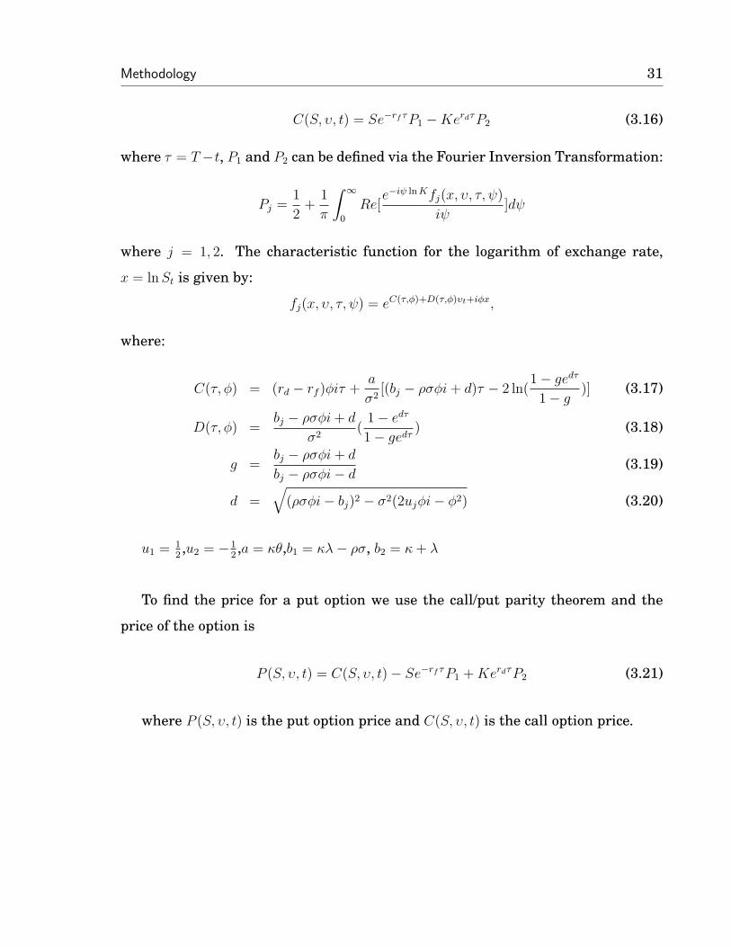
Methodology 31
C(S, υ, t) = Se−rf τP1 −KerdτP2 (3.16)
where τ = T−t, P1 and P2 can be defined via the Fourier Inversion Transformation:
Pj =1
2+
1
π
∫ ∞
0
Re[e−iψ lnKfj(x, υ, τ, ψ)
iψ]dψ
where j = 1, 2. The characteristic function for the logarithm of exchange rate,
x = lnSt is given by:
fj(x, υ, τ, ψ) = eC(τ,φ)+D(τ,φ)υt+iφx,
where:
C(τ, φ) = (rd − rf )φiτ +a
σ2[(bj − ρσφi+ d)τ − 2 ln(
1− gedτ
1− g)] (3.17)
D(τ, φ) =bj − ρσφi+ d
σ2(
1− edτ
1− gedτ) (3.18)
g =bj − ρσφi+ d
bj − ρσφi− d(3.19)
d =√
(ρσφi− bj)2 − σ2(2ujφi− φ2) (3.20)
u1 = 12,u2 = −1
2,a = κθ,b1 = κλ− ρσ, b2 = κ+ λ
To find the price for a put option we use the call/put parity theorem and the
price of the option is
P (S, υ, t) = C(S, υ, t)− Se−rf τP1 +KerdτP2 (3.21)
where P (S, υ, t) is the put option price and C(S, υ, t) is the call option price.
Methodology 32
3.4. Visual Basic and Excel in obtaining a closed
form solution for the Heston model
We use Visual Basic and Excel to fit the Heston model closed form solution. Evalu-
ating P1 and P2 involves the use of complex numbers which may be generally diffi-
cult to code in excel and VBA. For the numerical integration method, the Simpson
rule instead of the Gauss Quadrature is employed, which is relatively accurate and
is not hard to program in Excel-VBA. The input variables for the closed form includ-
ing stock spot price ST , strike price K, risk-free interest rate rd and rf , time step
which need to do integration and the five parameters υ, κ, θ, σ and ρ that needed to
be estimated. The VBA code for the Heston Model is found in the appendix.
3.5. Model Calibration
There are five parameters υ, κ, θ, σ and ρ that need to be estimated in the Heston
model. The change for each parameter will bring a big impact on the correctness
of the model, so the estimation of parameters becomes very important. A variety
of methods can be chosen. For instance, one can observe the real market data,
and use statistic tool to fit data in the Heston model (Ait-Sahila & Kimmel, 2005).
Monte Carlo simulation is another famous method to do the calibration, Alexander
(2010).
In this study we use a commonly used method called the Inverse Problem, which
means that the data is collected from the real market first, and then used to esti-
mate parameters. The most popular approach to solving this inverse problem is to
minimise the error or discrepancy between Heston model prices and real market
prices. This usually turns out to be a non-linear least-squares optimisation prob-
lem. More specifically, the squared differences between European option market
prices and that of the model are minimised over the parameter space. Assume Ω is
a set of realization for the parameters in the Heston model. For a call option that
is calculated from the Heston model, the optimization problem can be described as:
Methodology 33
MinS(Ω) = min(Ω)∑n
i=1(CHi − CM
i )2
Subject to:
2κθ > σ2
−1 < ρ < 1
κ > 0
0 < θ < 1
0 < σ < 1.
where CHi and CM
i are the ith call option price, respectively, calculated by the
Heston model and collected from the real market. N is the number of options that
are used to calibrate the model. Various softwares can be used in calibrating the
Heston model using the Inverse problem model. One of these is Matlab, however in
this study Excel solver was used as it is quick and produces fairly accurate results.
Excel Solver turns out to be very robust and reliable among all kinds of local op-
timizers, Mikhailov (2008). The method employed by Excel Solver is Generalized
Reduce Gradient (GRG) method. More detail on the Generalized reduced gradient
method is found in the appendix.
3.6. Comparison between the Heston Model and
the Garman-Kohlhagen model
3.6.1. Model accuracy
To check for model accuracy, the average relative percentage (ARP) method is em-
ployed. Respective ARP for the Heston and the Garman-Kohlhagen model are
computed. The model which has a small percentage error to six decimal places
is taken to be the better model. The mathematical expression for the percentage
error is given as:
Error =|Modelprice−Realprice|
|Realprice|× 100. (3.22)
Methodology 34
3.6.2. Model Fairness
Studies on the Garman-Kohlhagen reveal that the model tends to:
1. Overprice at the money options, that is where St ≈ K.
2. Underprice options at the ends in the money, St >> K or deep out of the
money St << K.
This is an indication that security price processes have “fat tails” ,i.e, a distribution
which has the probability of large changes in price St greater than those predicted
by the lognormal distribution. Further research shows that stochastic volatility
models address this limitation. We compare the option prices for the Heston model
and the Garman-Kohlhagen model to determine the model that produces fairer
results. The price for comparison with real market prices is determined from the
heston model after the model has been calibrated to find the approximate values
for its parametres.
3.7. Sensitivity Analysis of Heston model parame-
ters
For the Heston model to converge to the Garman-Kohlhagen model, volatility, σGK ,
should be equivalent to the square root of the volatility process, Vt, in the Heston
model. Once this condition is held constant we perform sensitivity analysis deter-
mine the impact of the Heston model parameters on option prices. One common
phenomenon is that the Garman-Kohlhagen model cannot account for variation in
exchange rates, in this regard, through sensitivity analysis we seek to determine if
the correlation coefficient, ρ can explain the skewness in exchange rates and also
if the volatility of volatility, σHeston, can explain the kurtosis of exchange rates. To
doing so, we hold ρ and σHeston constant respectively and observe if any significant
difference exist in between the Garman-Kohlhagen model and the Heston model.
Methodology 35
3.8. Option Pricing Application
Finally we develop a user friendly application for pricing foreign currency option.
The main tools used in developing the application are Visual basic and Microsoft
excel. The application developed should allow the user to choose a model to use in
determining the price of an option between the Garman-Kohlhagen model and the
Heston model.
3.9. Summary
Stochastic differential equations play a huge role in pricing foreign currency op-
tions. We will use stochastic differential equations to determine the foreign cur-
rency option prices as defined by the Heston model and the Garman-Kohlhagen
model (1983). The first part of this chapter served as an introduction to stochas-
tic differential equations and their application in option pricing. Furthermore we
will apply fourier transformations in solving the Heston model partial differential
equation so as to come up with a closed form solution for the Heston model. The for-
eign currency put option will be derived using the call/put parity principle. After
having found the closed solution, the Heston model is then callibrated using the
inverse problem method that is then solved using Excel Solver while employing
the Generalized Reduce Gradient (GRG) method. Another method we will employ
in pricing options in this project is the Garman Kohlhagen model, so included in
this chapter is a section that shows how the closed form solution for a call option
according to the Garman Kohlahagen is obtained. We will then perform a compar-
ison between the Heston model and the Garman Kohlhagen model to determine
a model that is better in giving accurate option prices and also in producing fair
option prices was done. Finally explained in this chapter is the use of excel and
Visual basic in developing an application for pricing foreign currency options in
Zimbabwe.
Chapter 4
Data Analysis, Simulations and
Results
4.1. Introduction
The Garman-Kohlhagen model has long been used to price foreign currency options
in both organised exchanges and over the counter markets. The main reason for
its adoption as the main foreign currency option pricing model is not because of its
accuracy or ability to explain flactuations in exchange rate, but beacuse of its sim-
plicity. Several researches have been done to determine a better pricing model than
the Garman-Kohlhagen model. In our case we use the Heston model. The Heston
model assumes that the volatility process for the model follows a stochastic process
which is modelled as a stochastic differential equation. Past studies have shown
that this assumption tends to produce better results than the Garman-Kohlhagen
model which assumes that the volatility process is constant. The main motiva-
tion of this chapter is to ascertain whether these studies have been true or not.
Furthermore after having produced the results for the comparison of both models
against the market option price, we then develop a user friendly application for
Data Analysis, Simulations and Results 37
pricing foreign currency options.
4.2. Data and data sources
In order to produce fairly accurate results the Heston model needs to be calibrated
so as to estimate numerical values for its parameters. In calibrating the Heston
model, the USD/ZAR pair was used to estimate ρ, σ, θ, υ and κ.
In determining the foreign currency option price using either the Heston model
or the Garman-Kohlhagen model, the following prevailing market data had to be
extracted from the foreign currency market. This data includes:
1. Exchange rate,
2. Domestic and Foreign interest rate, and
3. Strike price.
Daily exchange rates data from 2009 to 2013 was obtained from Old Mutual Zim-
babwe. This data contained the, opening, highest, lowest and closing price recorded
on that day. To obtain the prevailing exchange rate for the day we used the closing
price. Instead of using the whole dataset from 2009 to 2013, we extracted data for
the year 2013.
The US Treasury produces data for daily risk free interest rates. These rates are
used to determine the domestic interest rates used in this study. Foreign interest
rates, in this case the foreign currency being the South African rand, were obtained
from the Reserve bank of South Africa. The South African reserve bank produces
risk free interest rate on an annual basis, in this regard the foreign interest rate
for 2013 had a constant value of 5.5% per annum.
The Strike price data was obtained from the Johannesburg Stock Exchange’s for-
eign currency options market. European options are traded and exercised on spe-
cific dates. We used options with the following expiry dates:
• options that expire in 3 months,
Data Analysis, Simulations and Results 38
• 6 months currency options,
• 9 months currency options, and
• options that expire after 12 months.
Considering that this is raw data, we treated the data to ensure that it helped us
achieve our objectives.
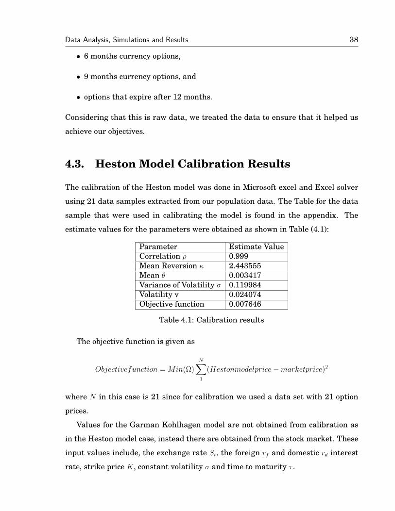
4.3. Heston Model Calibration Results
The calibration of the Heston model was done in Microsoft excel and Excel solver
using 21 data samples extracted from our population data. The Table for the data
sample that were used in calibrating the model is found in the appendix. The
estimate values for the parameters were obtained as shown in Table (4.1):
Parameter Estimate ValueCorrelation ρ 0.999Mean Reversion κ 2.443555Mean θ 0.003417Variance of Volatility σ 0.119984Volatility v 0.024074Objective function 0.007646
Table 4.1: Calibration results
The objective function is given as
Objectivefunction = Min(Ω)N∑1
(Hestonmodelprice−marketprice)2
where N in this case is 21 since for calibration we used a data set with 21 option
prices.
Values for the Garman Kohlhagen model are not obtained from calibration as
in the Heston model case, instead there are obtained from the stock market. These
input values include, the exchange rate St, the foreign rf and domestic rd interest
rate, strike price K, constant volatility σ and time to maturity τ .
Data Analysis, Simulations and Results 39
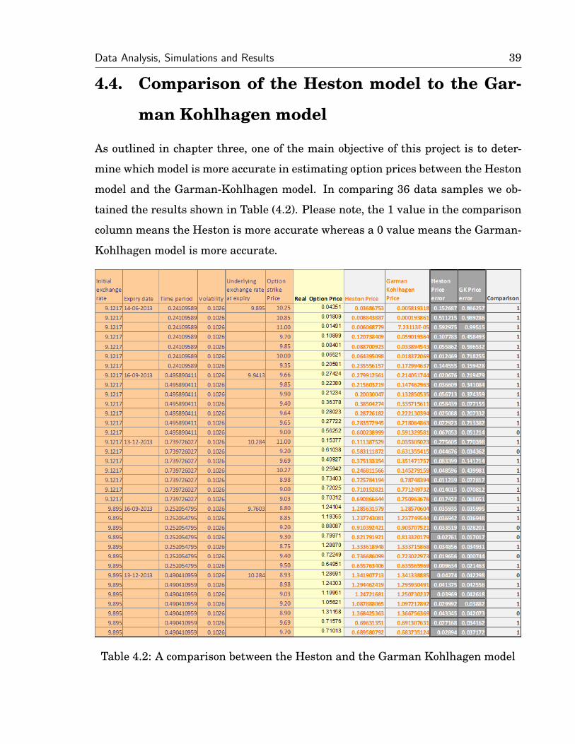
4.4. Comparison of the Heston model to the Gar-
man Kohlhagen model
As outlined in chapter three, one of the main objective of this project is to deter-
mine which model is more accurate in estimating option prices between the Heston
model and the Garman-Kohlhagen model. In comparing 36 data samples we ob-
tained the results shown in Table (4.2). Please note, the 1 value in the comparison
column means the Heston is more accurate whereas a 0 value means the Garman-
Kohlhagen model is more accurate.
Table 4.2: A comparison between the Heston and the Garman Kohlhagen model
Data Analysis, Simulations and Results 40
4.4.1. Interpretation of the table
Comparison between the Heston and Garman-Kohlhagen model
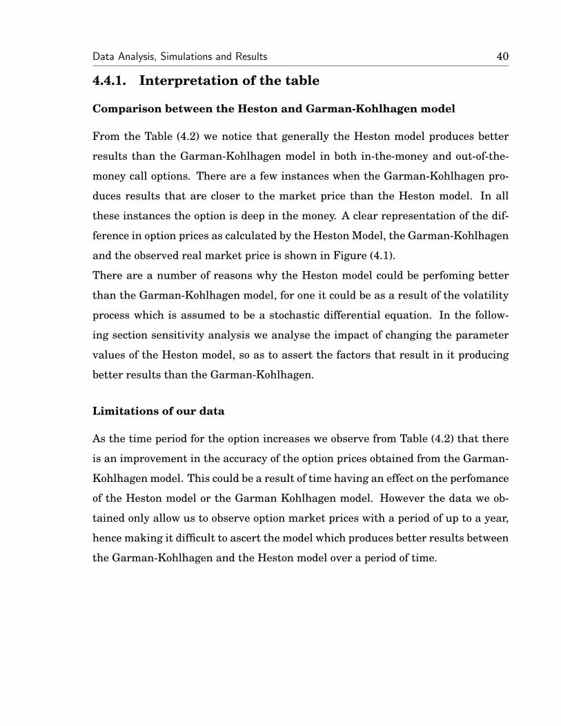
From the Table (4.2) we notice that generally the Heston model produces better
results than the Garman-Kohlhagen model in both in-the-money and out-of-the-
money call options. There are a few instances when the Garman-Kohlhagen pro-
duces results that are closer to the market price than the Heston model. In all
these instances the option is deep in the money. A clear representation of the dif-
ference in option prices as calculated by the Heston Model, the Garman-Kohlhagen
and the observed real market price is shown in Figure (4.1).
There are a number of reasons why the Heston model could be perfoming better
than the Garman-Kohlhagen model, for one it could be as a result of the volatility
process which is assumed to be a stochastic differential equation. In the follow-
ing section sensitivity analysis we analyse the impact of changing the parameter
values of the Heston model, so as to assert the factors that result in it producing
better results than the Garman-Kohlhagen.
Limitations of our data
As the time period for the option increases we observe from Table (4.2) that there
is an improvement in the accuracy of the option prices obtained from the Garman-
Kohlhagen model. This could be a result of time having an effect on the perfomance
of the Heston model or the Garman Kohlhagen model. However the data we ob-
tained only allow us to observe option market prices with a period of up to a year,
hence making it difficult to ascert the model which produces better results between
the Garman-Kohlhagen and the Heston model over a period of time.
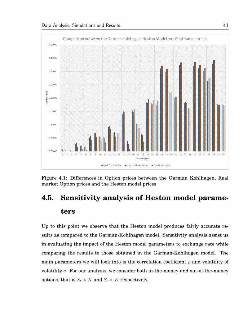
Data Analysis, Simulations and Results 41
Figure 4.1: Differences in Option prices between the Garman Kohlhagen, Realmarket Option prices and the Heston model prices
4.5. Sensitivity analysis of Heston model parame-
ters
Up to this point we observe that the Heston model produces fairly accurate re-
sults as compared to the Garman-Kohlhagen model. Sensitivity analysis assist us
in evaluating the impact of the Heston model parameters to exchange rate while
comparing the results to those obtained in the Garman-Kohlhagen model. The
main parameters we will look into is the correlation coefficient ρ and volatility of
volatility σ. For our analysis, we consider both in-the-money and out-of-the-money
options, that is St > K and St < K respectively.
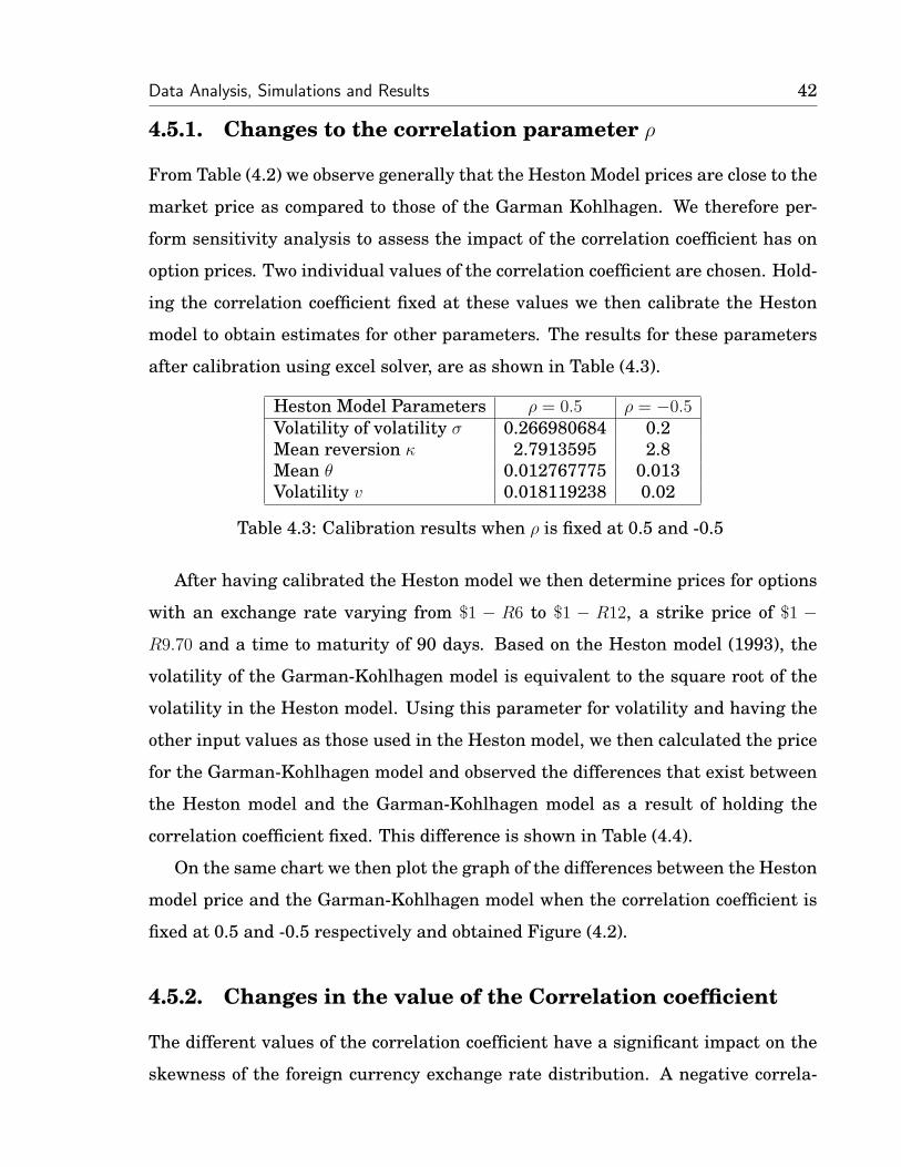
Data Analysis, Simulations and Results 42
4.5.1. Changes to the correlation parameter ρ
From Table (4.2) we observe generally that the Heston Model prices are close to the
market price as compared to those of the Garman Kohlhagen. We therefore per-
form sensitivity analysis to assess the impact of the correlation coefficient has on
option prices. Two individual values of the correlation coefficient are chosen. Hold-
ing the correlation coefficient fixed at these values we then calibrate the Heston
model to obtain estimates for other parameters. The results for these parameters
after calibration using excel solver, are as shown in Table (4.3).
Heston Model Parameters ρ = 0.5 ρ = −0.5Volatility of volatility σ 0.266980684 0.2Mean reversion κ 2.7913595 2.8Mean θ 0.012767775 0.013Volatility v 0.018119238 0.02
Table 4.3: Calibration results when ρ is fixed at 0.5 and -0.5
After having calibrated the Heston model we then determine prices for options
with an exchange rate varying from $1 − R6 to $1 − R12, a strike price of $1 −
R9.70 and a time to maturity of 90 days. Based on the Heston model (1993), the
volatility of the Garman-Kohlhagen model is equivalent to the square root of the
volatility in the Heston model. Using this parameter for volatility and having the
other input values as those used in the Heston model, we then calculated the price
for the Garman-Kohlhagen model and observed the differences that exist between
the Heston model and the Garman-Kohlhagen model as a result of holding the
correlation coefficient fixed. This difference is shown in Table (4.4).
On the same chart we then plot the graph of the differences between the Heston
model price and the Garman-Kohlhagen model when the correlation coefficient is
fixed at 0.5 and -0.5 respectively and obtained Figure (4.2).
4.5.2. Changes in the value of the Correlation coefficient
The different values of the correlation coefficient have a significant impact on the
skewness of the foreign currency exchange rate distribution. A negative correla-
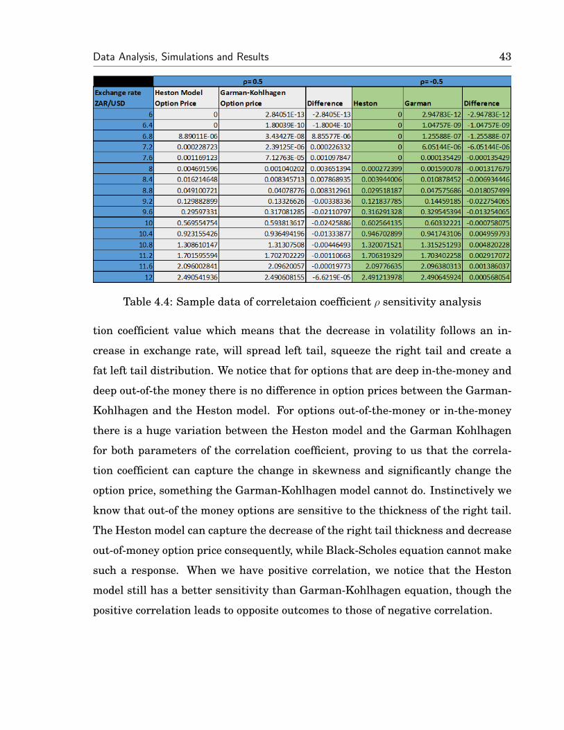
Data Analysis, Simulations and Results 43
Table 4.4: Sample data of correletaion coefficient ρ sensitivity analysis
tion coefficient value which means that the decrease in volatility follows an in-
crease in exchange rate, will spread left tail, squeeze the right tail and create a
fat left tail distribution. We notice that for options that are deep in-the-money and
deep out-of-the money there is no difference in option prices between the Garman-
Kohlhagen and the Heston model. For options out-of-the-money or in-the-money
there is a huge variation between the Heston model and the Garman Kohlhagen
for both parameters of the correlation coefficient, proving to us that the correla-
tion coefficient can capture the change in skewness and significantly change the
option price, something the Garman-Kohlhagen model cannot do. Instinctively we
know that out-of the money options are sensitive to the thickness of the right tail.
The Heston model can capture the decrease of the right tail thickness and decrease
out-of-money option price consequently, while Black-Scholes equation cannot make
such a response. When we have positive correlation, we notice that the Heston
model still has a better sensitivity than Garman-Kohlhagen equation, though the
positive correlation leads to opposite outcomes to those of negative correlation.
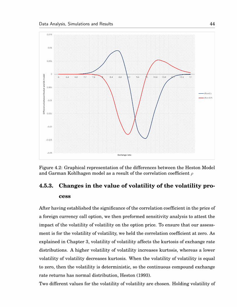
Data Analysis, Simulations and Results 44
Figure 4.2: Graphical representation of the differences between the Heston Modeland Garman Kohlhagen model as a result of the correlation coefficient ρ
4.5.3. Changes in the value of volatility of the volatility pro-
cess
After having established the significance of the correlation coefficient in the price of
a foreign currency call option, we then preformed sensitivity analysis to attest the
impact of the volatility of volatility on the option price. To ensure that our assess-
ment is for the volatility of volatility, we held the correlation coefficient at zero. As
explained in Chapter 3, volatility of volatility affects the kurtosis of exchange rate
distributions. A higher volatility of volatility increases kurtosis, whereas a lower
volatility of volatility decreases kurtosis. When the volatility of volatility is equal
to zero, then the volatility is deterministic, so the continuous compound exchange
rate returns has normal distribution, Heston (1993).
Two different values for the volatility of volatility are chosen. Holding volatility of
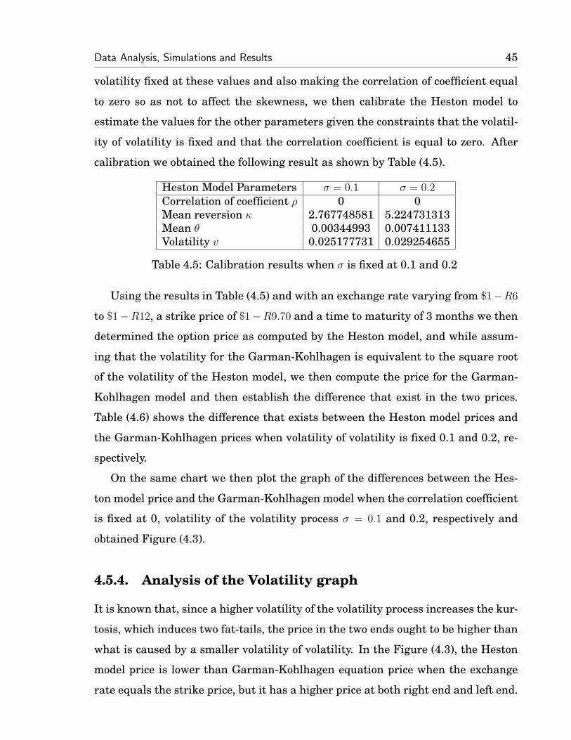
Data Analysis, Simulations and Results 45
volatility fixed at these values and also making the correlation of coefficient equal
to zero so as not to affect the skewness, we then calibrate the Heston model to
estimate the values for the other parameters given the constraints that the volatil-
ity of volatility is fixed and that the correlation coefficient is equal to zero. After
calibration we obtained the following result as shown by Table (4.5).
Heston Model Parameters σ = 0.1 σ = 0.2Correlation of coefficient ρ 0 0Mean reversion κ 2.767748581 5.224731313Mean θ 0.00344993 0.007411133Volatility v 0.025177731 0.029254655
Table 4.5: Calibration results when σ is fixed at 0.1 and 0.2
Using the results in Table (4.5) and with an exchange rate varying from $1−R6
to $1−R12, a strike price of $1−R9.70 and a time to maturity of 3 months we then
determined the option price as computed by the Heston model, and while assum-
ing that the volatility for the Garman-Kohlhagen is equivalent to the square root
of the volatility of the Heston model, we then compute the price for the Garman-
Kohlhagen model and then establish the difference that exist in the two prices.
Table (4.6) shows the difference that exists between the Heston model prices and
the Garman-Kohlhagen prices when volatility of volatility is fixed 0.1 and 0.2, re-
spectively.
On the same chart we then plot the graph of the differences between the Hes-
ton model price and the Garman-Kohlhagen model when the correlation coefficient
is fixed at 0, volatility of the volatility process σ = 0.1 and 0.2, respectively and
obtained Figure (4.3).
4.5.4. Analysis of the Volatility graph
It is known that, since a higher volatility of the volatility process increases the kur-
tosis, which induces two fat-tails, the price in the two ends ought to be higher than
what is caused by a smaller volatility of volatility. In the Figure (4.3), the Heston
model price is lower than Garman-Kohlhagen equation price when the exchange
rate equals the strike price, but it has a higher price at both right end and left end.
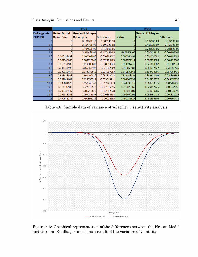
Data Analysis, Simulations and Results 46
Table 4.6: Sample data of variance of volatility σ sensitivity analysis
Figure 4.3: Graphical representation of the differences between the Heston Modeland Garman Kohlhagen model as a result of the variance of volatility
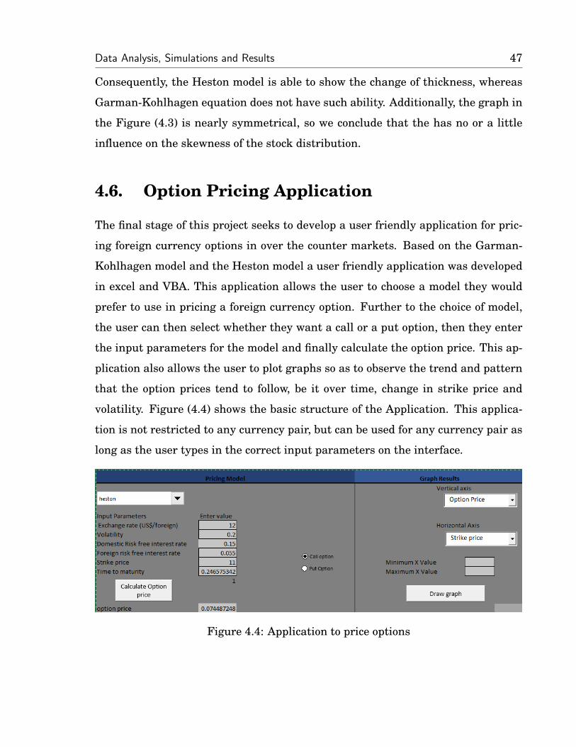
Data Analysis, Simulations and Results 47
Consequently, the Heston model is able to show the change of thickness, whereas
Garman-Kohlhagen equation does not have such ability. Additionally, the graph in
the Figure (4.3) is nearly symmetrical, so we conclude that the has no or a little
influence on the skewness of the stock distribution.
4.6. Option Pricing Application
The final stage of this project seeks to develop a user friendly application for pric-
ing foreign currency options in over the counter markets. Based on the Garman-
Kohlhagen model and the Heston model a user friendly application was developed
in excel and VBA. This application allows the user to choose a model they would
prefer to use in pricing a foreign currency option. Further to the choice of model,
the user can then select whether they want a call or a put option, then they enter
the input parameters for the model and finally calculate the option price. This ap-
plication also allows the user to plot graphs so as to observe the trend and pattern
that the option prices tend to follow, be it over time, change in strike price and
volatility. Figure (4.4) shows the basic structure of the Application. This applica-
tion is not restricted to any currency pair, but can be used for any currency pair as
long as the user types in the correct input parameters on the interface.
Figure 4.4: Application to price options
Data Analysis, Simulations and Results 48
4.7. Summary
In this chapter, Data analysis, Simulations and Results, we consolidated the method
described in Chapter 3 by appliying it to a data set obtained from the JSE, Old Mu-
tual Zimbabwe and the internet. To obtain accurate results of the Heston model
we calibrated the model using the inverse method in Excel. After having calibrated
the Heston model and obtained fairly accurate results for the input parameters, we
then evaluated the perfomance of the Heston model as compared to the Garman
Kohlhagen and we observed that the Heston model produces better results than
the Garman-Kohlhagen. We then went a step further to perform sensitivity anal-
ysis of the model so as to determine the individual impact of ρ and σ on the option
price. Finally we developed a user friendly application for pricing foreign currency
options. This application allows the user to choose between the Heston model and
the Garman Kohlhagen model.
Chapter 5
Conclusions and
Recommendations
5.1. Introduction
The main aim of this project was to develop a user friendly application that can be
used to price foreign currency options in over the counter markets. In developing
the application, two foreign currency pricing models were used, the Heston model
and the Garman-Kohlhagen model which is used widely in the world in determin-
ing the price of an option. The Heston model (1993) on the other hand has been
used here and there in determining the price of an option but its impact has not
been much as compared to the Garman-Kohlhagen model as there is a challenge
in calibrating the model for its input parameters or understanding the long partial
differential equation from which the model is derived. In this chapter however, we
outline the impact that the developed application can have in advancing the use of
foreign currency options in Zimbabwe.
Conclusions and Recommendations 50
5.2. Conclusions and Recommendations from the
study
The Heston model produces fairly accurate results in pricing foreign currency op-
tions as compared to the Garman-Kohlhagen(1983) model. One of the main objec-
tives that financial engineers seek to achieve in developing foreign currency option
pricing models is to:
1. Deteremine a fair price for an option, and
2. Develop an accurate model comparing model values to observed values.
We notice that the Heston model produces fairly accurate results, because from a
sample of 36 samples of call options, more than 25 results proved that the Heston
model was a better pricing model as compared to the Garman Kohlhagen model.
However, for options that are deep in-the-money or deep out-of-the-money, the op-
tion price as calculated by the Heston model is not in anyway different from that
of the Garman-Kohlhagen model.
Based on the counter’s risk profiles they can use either the Heston model or the
garman Kohlhagen model, however we recommend that the user uses the Heston
model and just compare with the Garman Kohlhagan model, to ensure that the
price is in an acceptable range. The Heston model’s correlation coefficient param-
eter enable it to account for skewness thereby explaining the volatility smile phe-
nomenon, something the Garman Kohlhagen model cannot do. By accounting for
skewness, the Heston model ensures that any change in currency exchange rate,
results in a significant change in the price of the option, thereby making it a better
suited model.
The Garman-Kohlhagen model has been very successful in being used for pric-
ing currency options worldwide because of its simplicity. To ensure that the Heston
model, meets the simplicity condition, an user friendly application, that enables
the user to choose either the Garman-Kohlhagen model or the Heston model, could
Conclusions and Recommendations 51
be a major breakthrough for the Heston model, as various players will begin to
see its advantages as an option pricing tool. Depending on who is determining
the price of an option, for a call option, the writer of the option can use a model
that overprices the call option so as to ensure that in the even that the option is
in-the-money, the writer will not bear unnecessary losses.
5.3. Conclusion
Almost on a daily basis, traders, be it supermarkets, manufacturing companies,
small scale traders, leave the country to go import foreign products and raw mate-
rials for their operations or for resale to local buyers. Their business is very much
affected by flactuations in exchange rates. In the event that the US dollar, losses
value against the foreign currency, the trader’s business is affected and most of the
times, the trader has no choice but to increase the price of goods, thereby affecting
the final consumer and the economy as a whole. Foreign currency options are a very
good way in which investors can protect themselves against flactuations in foreign
exchange rates. The market has long awaited for these instruments and this could
be good business for financial institutions which are also struggling to raise money
as they have a few financial products on offer. Other than being used for pricing
foreign currency options, the pricing application developed in this project can also
be used as a basis for pricing foreign currency futures, the bank playing the part of
both the clearing house and the counter party.
Bibliography
Adams, P. and Wyatt, S., Biases in Option Prices - Evidence from the Foreign-Currency Option Market. Journal of Banking and Finance, 11: 9-562, 1987a.
Adams, P. and Wyatt, S., On the Pricing of European and American Foreign-Currency Call Options. Journal of International Money and Finance, 6: 315-338,1987b.
Amin, K. and Bodurtha, J., Discrete-Time Valuation of American Options withStochastic Interest Rates. The Review of Financial Studies, 819: 3-234, 1995.
Amin, K. and Ng, V., Option Valuation with Systematic Stochastic Volatil-ity.Journal of Finance, 48, 881-910,1993.
Anatoliy, S., Stochastic Volatility and Change of Time: Overview,(September2010).
Bakshi, G., and Chen, Z., Equilibrium Valuation of Foreign-Exchange Claims.Journal of Finance, 52, 799-826, 1997.
Bakshi, G., Cao, C., and Chen, Z, Empirical Performance of Alternative OptionPricing Models. The Journal of Finance, 52:2003-2049, 1997.
Bates, D., Jumps and Stochastic Volatility - Exchange-Rate Processes Implicit inDeutsche Mark Options. Review of Financial Studies, 9: 69-107, 1996.
Biger, N. and Hull, J., The valuation of currency options. Financial Management,12, 24-28, 1983.
Blake, D., Option pricing model: Journal of the Institute of Actuaries (1886-1994),Vol. 116(3): 537-558,(December 1989).
Black, F., and Karasinski, P., Bond and Option Pricing When Short Rates AreLognormal. Financial Analysts Journal, 47, 52-59, 1991.
Black, F., and Scholes, M., The pricing of Options and Corporate liabilities TheJournal of political economy, vol 81(3): 637-654, (May-June 1973).
Black, F., Studies of stock market changes, Proceedings 1976 of the AmericanStatistical Association, Business and Economics Statistics Section 177, 1976.
BIBLIOGRAPHY 53
Brennan, M., and Schwartz, E., An Equilibrium Model of Bond Prices and A Testof Market Effciency. Journal of Financial and Quantitative Analysis, 17: 301-329,1982.
Chang, C., Efficient Procedures for The Valuation and Hedging of American Cur-rency Options with Stochastic Interest Rates. Journal of Multinational FinancialManagement, 11: 241-268, 2001.
Chesney, M. and Jeanblanc, M., Pricing American Currency Options in A jumpdiffusion Model. Applied Mathematical Finance, 11, 207-225, 2004.
Chensey, M. and Scott, L., Pricing European Currency options: a comparison ofthe modified black scholes model and the random variance model: Journal of fi-nancial and quantitative analysis volume 24(3), (September 1989).
Chisholm, M.A., Derivatives Demystified: A Step by Step Guide in Forwards,Swaps, Futures and Options, John Wiley and Sons Ltd. Southern gate England,2004.
Choi, S. and Marcozzi, M., A Numerical Approach to American Currency OptionValuation. Journal of Derivatives, 9, 19-29, 2001.
Choi, S. and Marcozzi, M D., The Valuation of Foreign Currency Options underStochastic Interest Rates. Computers and Mathematics with Applications, 46:741-749, 2003.
Clark, P., Tamirisa, N. and Wei, S. Exchange Rate Volatility and Trade Flows-Some New Evidence. International Monetary Fund, 2004.
Clifford A.B. and Roma, A., Stochastic Volatility Option pricing Journal of Finan-cial and quantitative analysis Volume 2(4):589-607, 1984.
Cox, J C., Ingersoll, J E. and Ross, S.A, An Intertemporal General EquilibriumModel of Asset Prices. Econometrica, 53, 363-384, 1985.
Cross, S., All About The Foreign Exchange Market in The United States.Tech.rept. Federal Reserve Bank of New York, 1998.
Dodd, R., Derivative Markets: Sources of Vulnerability in U.S.Financial Markets.Financial Policy Forum Derivatives Study Centre,Washington DC, 2004.
Doffou, S. and Hilliard, J E. Pricing Currency Options Under Stochastic InterestRates and Jump-diffusion Processes. The Journal of Financial Research, 24,565-585, 2001.
Duan, J.C. and Wei, J., Pricing Foreign Currency and Cross-Currency OptionsUnder GARCH. Journal of Derivatives, 7: 51-63, 1999.
Dupoyet, B., Information Content of Cross-Sectional Option Prices: A Comparisonof Alternative Currency Option Pricing Models on the Japanese Yen. The Journalof Futures Markets, 26: 33-59, 2006.
BIBLIOGRAPHY 54
Effenberger, D., Credit Derivatives, Effects on the Stability of Financial Mar-kets,Deutsche Bank Research, 2004.
Eisler, Z., Perello, J. and Masoliver, J., Volatility: a hidden Markov process infinancial time series, Physical Review E 76: 11, 2007.
Fouque, J.P, Papanicolaouy, G. and Sircarz, K.R., Stochastic Volatility Correctionto Black-Scholes (July 1999).
Garman, M., and Kohlhagen, S., Foreign Currency Option Values. Journal ofIn-ternational of Money and Finance, 2:231-237, 1983.
Geske, R., and Johnson, H., The American Put Option Valued Analytically. TheJournal of Finance, 39: 1511-1524, 1984.
Gibson, R., Option Valuation, New York McGraw hill, Journal of Finance,:959-976, (July,1991).
Grabbe, J. The Pricing of Call and Put Options on Foreign-Exchange. Journal ofInternational Money and Finance, 2, 239-253, 1983.
Grabbe, J., The Pricing of Call and Put Options on Foreign-Exchange. Journal ofInternational Money and Finance, 2, 239-253, 1983.
Heath, D., Jarrow, R., and Morton, A. Bond pricing and the term structure ofinterest rates: A new methodology for contingent claim valuation. Econometrica,60, 77-105, 1992.
Heston, S L., A Closed-Form Solution for Options with Stochastic Volatility withApplications to Bond and Currency Options. Review of Financial Studies,6, 327-343,1993.
Hilliard, J E., Madura, J., and Tucker, A L., Currency Option Pricing withStochastic Domestic and Foreign Interest Rates. Journal of Financial and Quan-titative Analysis, 26(2), 139-151,1991.
Hobson, D., Statistics in Finance. London: Arnold, 1998.
Hull, J., Options, Futures, and Other Derivative Securities. fifth edn.Englewood-Cliff, N.J.: Prentice-Hall, 2002.
Hull, J. and White, A., Numerical Procedures for Implementing Term StructureModels: Single Factor Models. Journal of Derivatives, 2, 7-19, 1994a.
Hull, J. and White, A., Numerical Procedures for Implementing Term StructureModels: Two Factor Models. Journal of Derivatives, 2, 37-47,1994b .
Hull, J., Options, Futures and other Derivatives, 4th Edition, N J, Prentice Hall,2001.
Hunt, P. and Kennedy, J., Financial Derivatives in Theory and Practice. Chich-ester: John Wiley and Sons, 2005.
BIBLIOGRAPHY 55
James, F.M and John, W., Labuszewski: Modifying the Black-Scholes OptionPricing Model for Alternative Underlying Instruments Financial Analysts Jour-nal,Vol. 40(6): 23-27+30, (Nov. - Dec., 1984).
Johnson and Shanno., Option pricing when the variance is changing: Journaloffiancial and quantitative analysis 22:1173-1186, (June 1987)
Kaushik L Amin and Robert A Jarrow: Pricing foreign currency options understochastic interest rates, 1991.
Kallianpur, G. and Karandikar, R. Introduction to Option Pricing Theory.Boston:Birkhaauser, 2000.
Longstaff, F. and Schwartz, E,. Interest Rate Volatility and The Term Structure:A Two Factor General Equilibrium Model. The Journal of Finance, 47: 1259-1282,1992.
Low, B. and Zhang, S., The Volatility Risk Premium Embedded in Currency Op-tions. Journal of Financial and Quantitative Analysis, Dec: 803-832, 2000b.
Marsh, T.A. and Rosenfeld, E.R., Stochastic processes for interest rates and equi-librium bond prices. Journal of Finance 38: 635-46, 1983.
Masoliver, J. and Perello, J., Multiple time scales and the exponential Ornstein-Uhlenbeck stochastic volatility model, Quantitative Finance 6: 423-433, 2006.
Melino, A. and Turnbull, S., The Pricing of Foreign Currency Options, CanadianJournal of Economics, 24, 251-281, 1991.
Merton, R., Theory of Rational Option Pricing. Bell Journal of Economics andManagement Science, 4:141-183, 1973.
Nawalkha, S K. and Chambers, D R., A Note on Currency Option Pric-ing.International Review of Financial Analysis, 4(1), 81-84, 1995.
Rodgers S., Zimbabwe Independent Newspaper, (14 June 2013).
Rubinstein, M., Nonparametric Tests of Alternative Option Pricing Models UsingAll Reported Trades and Quotes on the 30 Most Active CBOE Option Classes fromAugust 23, 1976 through August 31, 1978,Journal of Finance, 40, 455-480, 1985.
Scott L.O., Option pricing when the variance changes randomly: Theory, Estima-tion and application Journal of financial and quantitative analysis 22, 419-438,(Dec 1987).
Shastri, K. and Tandon, K., Valuation of American option on foreign currency.Journal of Banking and Finance, 11: 245-269, 1987.
Stein, E. M. and Stein, J. C., Stock Price Distributions with Stochastic Volatility:An Analytic Approach, Review of Financial Studies, 4:727-752, 1991.
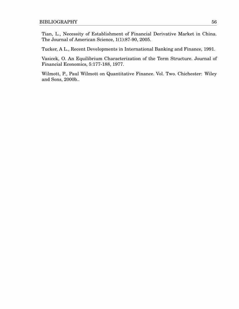
BIBLIOGRAPHY 56
Tian, L., Necessity of Establishment of Financial Derivative Market in China.The Journal of American Science, 1(1):87-90, 2005.
Tucker, A L., Recent Developments in International Banking and Finance, 1991.
Vasicek, O. An Equilibrium Characterization of the Term Structure. Journal ofFinancial Economics, 5:177-188, 1977.
Wilmott, P., Paul Wilmott on Quantitative Finance. Vol. Two. Chichester: Wileyand Sons, 2000b..
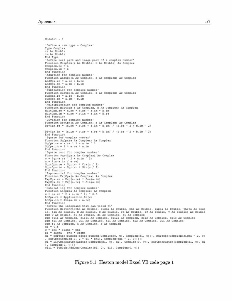
Appendix 57
Figure 5.1: Heston model Excel VB code page 1
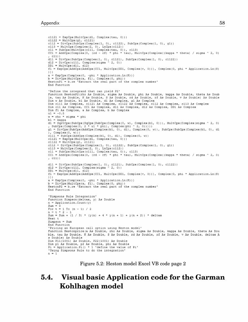
Appendix 58
Figure 5.2: Heston model Excel VB code page 2
5.4. Visual basic Application code for the GarmanKohlhagen model
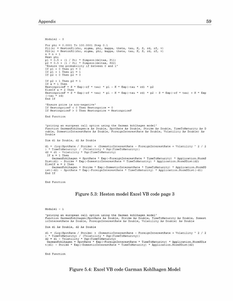
Appendix 59
Figure 5.3: Heston model Excel VB code page 3
Figure 5.4: Excel VB code Garman Kohlhagen Model
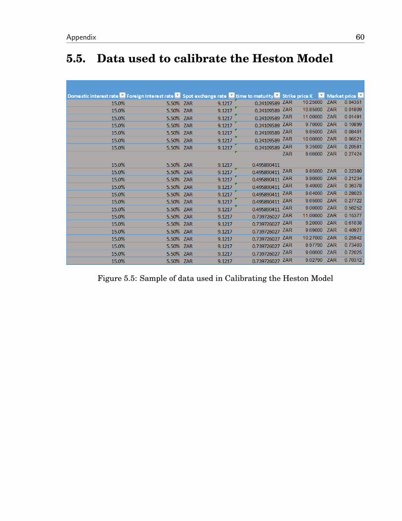
Appendix 60
5.5. Data used to calibrate the Heston Model
Figure 5.5: Sample of data used in Calibrating the Heston Model
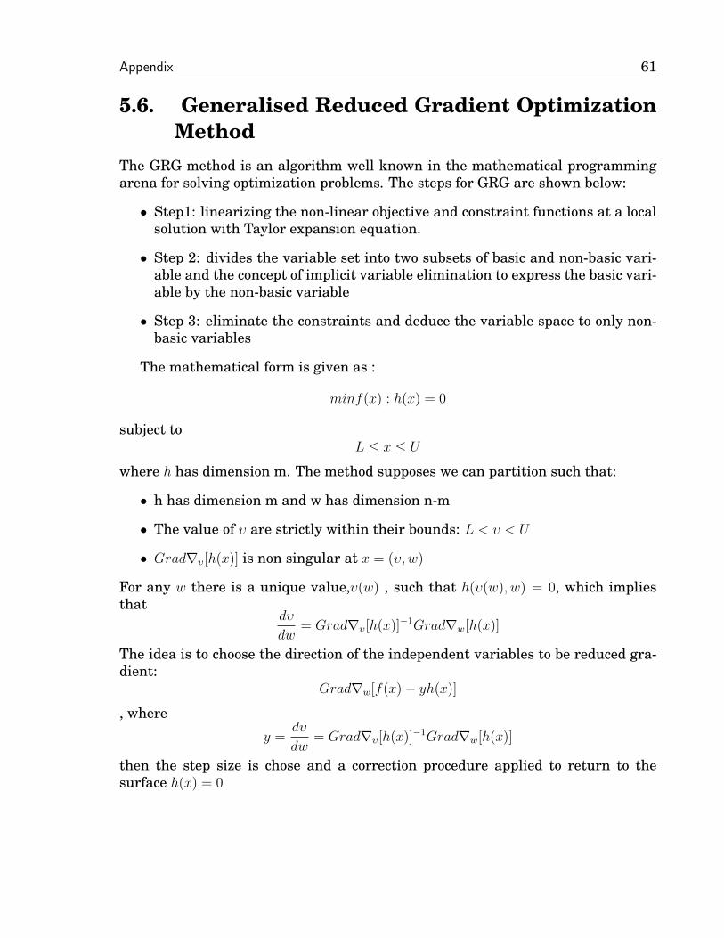
Appendix 61
5.6. Generalised Reduced Gradient OptimizationMethod
The GRG method is an algorithm well known in the mathematical programmingarena for solving optimization problems. The steps for GRG are shown below:
• Step1: linearizing the non-linear objective and constraint functions at a localsolution with Taylor expansion equation.
• Step 2: divides the variable set into two subsets of basic and non-basic vari-able and the concept of implicit variable elimination to express the basic vari-able by the non-basic variable
• Step 3: eliminate the constraints and deduce the variable space to only non-basic variables
The mathematical form is given as :
minf(x) : h(x) = 0
subject toL ≤ x ≤ U
where h has dimension m. The method supposes we can partition such that:
• h has dimension m and w has dimension n-m
• The value of υ are strictly within their bounds: L < υ < U
• Grad∇υ[h(x)] is non singular at x = (υ, w)
For any w there is a unique value,υ(w) , such that h(υ(w), w) = 0, which impliesthat
dυ
dw= Grad∇υ[h(x)]
−1Grad∇w[h(x)]
The idea is to choose the direction of the independent variables to be reduced gra-dient:
Grad∇w[f(x)− yh(x)]
, where
y =dυ
dw= Grad∇υ[h(x)]
−1Grad∇w[h(x)]
then the step size is chose and a correction procedure applied to return to thesurface h(x) = 0