A Fast UTD-Based Method for the Analysis of Multiple ... - MDPI

symmetryS S

Article

A Fast UTD-Based Method for the Analysis ofMultiple Acoustic Diffraction over a Series ofObstacles with Arbitrary Modeling, Heightand Spacing

Domingo Pardo-Quiles and José-Víctor Rodríguez *

Departamento de Tecnologías de la Información y las Comunicaciones, Universidad Politécnica de Cartagena,E30202 Cartagena, Spain; [email protected]* Correspondence: [email protected]

Received: 25 March 2020; Accepted: 17 April 2020; Published: 21 April 2020��

Abstract: A uniform theory of diffraction (UTD)-based method for analysis of the multiple diffractionof acoustic waves when considering a series of symmetric obstacles with arbitrary modeling, heightand spacing is hereby presented. The method, which makes use of graph theory, funicular polygonsand Fresnel ellipsoids, proposes a novel approach by which only the relevant obstacles and pathsof the scenario under study are considered, therefore simultaneously providing fast and accurateprediction of sound attenuation. The obstacles can be modeled either as knife edges, wedges, widebarriers or cylinders, with some other polygonal diffracting elements, such as doubly inclined, T- orY-shaped barriers, also considered. In view of the obtained results, this method shows good agreementwith previously published formulations and measurements whilst offering better computationalefficiency, thus allowing for the consideration of a large number of obstacles.

Keywords: multiple sound diffraction; uniform theory of diffraction; knife edges; wide barriers;funicular profile; graph theory

1. Introduction

Different approaches have been carried out for the analysis of the acoustic wave diffraction causedby multiple obstacles. These approaches are typically based on boundary element methods (BEMs) [1],parabolic equation methods [2], the geometrical/uniform theory of diffraction (GTD/UTD) [3–8] orempirical formulae [9]. Among such methods, the GTD/UTD offers reduced mathematical complexityby entirely explaining the problem of wave diffraction in terms of rays, thereby considerably shorteningthe computation time.

Keller published the GTD [10] about 60 years ago and it is accurate for most practical casesproviding that the sound wavelength is smaller than the obstacle dimensions. However, this theoryfails in the vicinity of shadow boundaries (e.g., when the source, obstacle and receiver lie within astraight line). This shortcoming was later solved by Kouyoumjian and Pathak [11] by the proposal ofthe UTD, whose formulation is also applicable at shadow and reflection boundaries. This formulationallows for the multiple diffraction of acoustic waves in such environments where a set of identicaldiffracting obstacles are evenly spaced and can be of special relevance (e.g., the rows of seats incommon auditoriums or concert halls). In this sense, some of the authors of this study have recentlypublished works [7,8] where two-dimensional (2D) UTD formulations for such types of environmentshave been presented.

On the other hand, the analysis of the acoustic diffraction caused by obstacles of arbitrary heightand spacing can also be of great importance in many practical applications. In this sense, Pierce

Symmetry 2020, 12, 654; doi:10.3390/sym12040654 www.mdpi.com/journal/symmetry

http://www.mdpi.com/journal/symmetry

http://www.mdpi.com

https://orcid.org/0000-0003-3240-2568

https://orcid.org/0000-0002-3298-6439

http://www.mdpi.com/2073-8994/12/4/654?type=check_update&version=1

http://dx.doi.org/10.3390/sym12040654

http://www.mdpi.com/journal/symmetry

Symmetry 2020, 12, 654 2 of 24

developed an asymptotic solution to solve the diffraction around a wedge or a wide barrier, which isbased on the concepts of GTD [3], as well as an exact formulation together with Hadden for sounddiffraction over screens and wedges [12]. Later, Kawai proposed a GTD/UTD solution based on Pierce’sformulation for the analysis of sound diffraction by a many-sided barrier or pillar [4]. Kim et al.presented a GTD-based solution for the study of multiple acoustic diffraction caused by multiplewedges, barriers and polygonal-like shapes [5]. Finally, Min and Qiu proposed a GTD method foranalyzing sound diffraction around rigid, parallel, wide barriers [6].

Nevertheless, the main limitation of the above-mentioned works lies in the highly demandingcomputing requirements when a large number of obstacles is to be analyzed. Moreover, despite thewidely different approaches and studies on multiple acoustic diffraction, to the best of the authors’knowledge, there is not yet an accurate and general solution for multiple sound diffraction that cantake into consideration obstacles with arbitrary modeling, height and spacing.

In this paper, contrary to previous works of the authors [7,8] where only acousticmultiple-diffraction over obstacles of equal shape, height and spacing was analyzed, an innovativeUTD-based method for the analysis of the multiple diffraction of acoustic waves when consideringa series of symmetric obstacles with arbitrary modeling, height and spacing is presented. This way,the scenario considered in previous studies published by the authors not only is extended in terms ofthe possible shape, height and location of the obstacles (that is, in this work, those parameters canvary from one obstacle to another within the same array) but also the analysis is carried out from afully different approach. In this sense, the formulations presented in [7] and [8] were based on radiowave recursive relations emerging from the application of both UTD and physical optics (PO) theories.However, the method hereby presented is a pure-UTD acoustic approach which makes use of graphtheory, funicular polygons and Fresnel ellipsoids, so that only the relevant obstacles and paths ofa complex scenario are considered, therefore providing a fast, computationally efficient—while atthe same time accurate—prediction of sound attenuation. On this basis, a great number of obstacles(including neighboring ones of equal height) can be analyzed in an acceptable time and such obstaclescan be modeled either as knife edges, wedges, wide barriers or cylinders, as well as some otherpolygonal diffracting elements, such as T- or Y-shaped barriers.

2. Theoretical Method

The theoretical method proposed in this work is a UTD ray-based solution developed to analyzemultiple acoustic diffraction (and also reflections) of spherical waves in scenarios, which can includeparallel wide barriers, screens (knife edges), wedges, cylinders and polygonal shapes, such as T or Ybarriers. An example of such a configuration can be observed in Figure 1.

Symmetry 2020, 12, x FOR PEER REVIEW 2 of 25

On the other hand, the analysis of the acoustic diffraction caused by obstacles of arbitrary height and spacing can also be of great importance in many practical applications. In this sense, Pierce developed an asymptotic solution to solve the diffraction around a wedge or a wide barrier, which is based on the concepts of GTD [3], as well as an exact formulation together with Hadden for sound diffraction over screens and wedges [12]. Later, Kawai proposed a GTD/UTD solution based on Pierce’s formulation for the analysis of sound diffraction by a many-sided barrier or pillar [4]. Kim et al. presented a GTD-based solution for the study of multiple acoustic diffraction caused by multiple wedges, barriers and polygonal-like shapes [5]. Finally, Min and Qiu proposed a GTD method for analyzing sound diffraction around rigid, parallel, wide barriers [6].

Nevertheless, the main limitation of the above-mentioned works lies in the highly demanding computing requirements when a large number of obstacles is to be analyzed. Moreover, despite the widely different approaches and studies on multiple acoustic diffraction, to the best of the authors’ knowledge, there is not yet an accurate and general solution for multiple sound diffraction that can take into consideration obstacles with arbitrary modeling, height and spacing.

In this paper, contrary to previous works of the authors [7,8] where only acoustic multiple-diffraction over obstacles of equal shape, height and spacing was analyzed, an innovative UTD-based method for the analysis of the multiple diffraction of acoustic waves when considering a series of symmetric obstacles with arbitrary modeling, height and spacing is presented. This way, the scenario considered in previous studies published by the authors not only is extended in terms of the possible shape, height and location of the obstacles (that is, in this work, those parameters can vary from one obstacle to another within the same array) but also the analysis is carried out from a fully different approach. In this sense, the formulations presented in [7] and [8] were based on radio wave recursive relations emerging from the application of both UTD and physical optics (PO) theories. However, the method hereby presented is a pure-UTD acoustic approach which makes use of graph theory, funicular polygons and Fresnel ellipsoids, so that only the relevant obstacles and paths of a complex scenario are considered, therefore providing a fast, computationally efficient—while at the same time accurate—prediction of sound attenuation. On this basis, a great number of obstacles (including neighboring ones of equal height) can be analyzed in an acceptable time and such obstacles can be modeled either as knife edges, wedges, wide barriers or cylinders, as well as some other polygonal diffracting elements, such as T- or Y-shaped barriers.

2. Theoretical Method

The theoretical method proposed in this work is a UTD ray-based solution developed to analyze multiple acoustic diffraction (and also reflections) of spherical waves in scenarios, which can include parallel wide barriers, screens (knife edges), wedges, cylinders and polygonal shapes, such as T or Y barriers. An example of such a configuration can be observed in Figure 1.

Figure 1. Example of a scenario with obstacles of arbitrary shape, height and location.

The method is 2D, for which all these obstacles are assumed to be infinitely long. Moreover, the first-order diffracted field of the rays will be considered, as well as perfectly reflecting (ρ = 1) (acoustically hard) materials. However, the proposed method can be easily extended for specific input impedances, since the reflection coefficients as a function of the frequency are well known.

Figure 1. Example of a scenario with obstacles of arbitrary shape, height and location.

The method is 2D, for which all these obstacles are assumed to be infinitely long. Moreover,the first-order diffracted field of the rays will be considered, as well as perfectly reflecting (ρ = 1)(acoustically hard) materials. However, the proposed method can be easily extended for specific inputimpedances, since the reflection coefficients as a function of the frequency are well known.

Symmetry 2020, 12, 654 3 of 24

As a result, the total diffracted (and reflected on the floor/ground) complex pressure field at thereceiver R from a source S will be the summation of the overall rays impinging on R and coming fromall the possible paths [10,11]:

φtRx =n∑

i = 1

φi(S, R) (1)

where φi(S, R) is the complex received field of an individual ray from the source S to the receiverR following one of the selected n possible paths. S is assumed as a point source which generates aspherical wave front within an ideal isotropic (uniform) medium such as air, whereas the receiver (R)of the acoustic field would be a listener with an isotropic pattern having unity gain. The phase is takeninto consideration for each signal traversing each path, taking advantage of the GTD/UTD theory thatcombines the representation of rays with the diffraction phenomenon, thereby allowing the calculationof the field at the receiver as the vector resulting from the addition of the fields corresponding toeach ray.

2.1. Selection of Nodes of the Scenario

In the first stage of the method, the profile under research is entered by defining the heights,spacing, type or shape of each obstacle (e.g., knife edge, wedge, cylinder, wide-barrier or polygonalelement) as well as the parameters corresponding to the type of obstacle, if applicable (e.g., interiorangles for wedges, radii for cylinders or widths for wide barriers).

For this purpose, firstly, it is then required to identify the initial ‘nodes’ taking part of the arbitraryprofile, starting from the source up to the receiver. This task is undertaken from the definition of thescenario itself due to the fact that each obstacle can be really composed by either single (knife edges,wedges, cylinders) or connected nodes (wide barriers, T- and Y-shaped, doubly inclined). In order toillustrate the theoretical method, the example shown in Figure 2 will be considered, where a series ofdifferent obstacles are present. Specifically, three knife edges, one T-shaped obstacle, one wide barrier,two wedges and one cylinder. The interior angles of the wedges are 20◦ (wedge on the left) and 10◦

(wedge on the right). The radius of the cylinder is 0.2 m. The source and the receiver appear in red inthe profile.


As a result, the total diffracted (and reflected on the floor/ground) complex pressure field at the receiver R from a source S will be the summation of the overall rays impinging on R and coming from all the possible paths [10,11]:

ϕ = ϕ (𝑆, 𝑅) (1)

where 𝜙 (𝑆, 𝑅) is the complex received field of an individual ray from the source S to the receiver R following one of the selected n possible paths. S is assumed as a point source which generates a spherical wave front within an ideal isotropic (uniform) medium such as air, whereas the receiver (R) of the acoustic field would be a listener with an isotropic pattern having unity gain. The phase is taken into consideration for each signal traversing each path, taking advantage of the GTD/UTD theory that combines the representation of rays with the diffraction phenomenon, thereby allowing the calculation of the field at the receiver as the vector resulting from the addition of the fields corresponding to each ray.

2.1. Selection of Nodes of the Scenario

In the first stage of the method, the profile under research is entered by defining the heights, spacing, type or shape of each obstacle (e.g., knife edge, wedge, cylinder, wide-barrier or polygonal element) as well as the parameters corresponding to the type of obstacle, if applicable (e.g., interior angles for wedges, radii for cylinders or widths for wide barriers).

For this purpose, firstly, it is then required to identify the initial ‘nodes’ taking part of the arbitrary profile, starting from the source up to the receiver. This task is undertaken from the definition of the scenario itself due to the fact that each obstacle can be really composed by either single (knife edges, wedges, cylinders) or connected nodes (wide barriers, T- and Y-shaped, doubly inclined). In order to illustrate the theoretical method, the example shown in Figure 2 will be considered, where a series of different obstacles are present. Specifically, three knife edges, one T-shaped obstacle, one wide barrier, two wedges and one cylinder. The interior angles of the wedges are 20° (wedge on the left) and 10° (wedge on the right). The radius of the cylinder is 0.2 m. The source and the receiver appear in red in the profile.

Figure 2. Example of extraction of nodes from a scenario built by three knife edges, one T-shaped obstacle, one wide barrier, two wedges and one cylinder. The interior angles of the wedges are 20° (wedge on the left) and 10° (wedge on the right). The radius of the cylinder is 0.2 m. The source and the receiver appear in red in the profile.

The same process could be followed with any other scenario, either simpler or more complex. The difference would be the processing time required to get the global complex pressure field received by the listener, which is further discussed in Section 3. What is more, even complex, irregular

Figure 2. Example of extraction of nodes from a scenario built by three knife edges, one T-shapedobstacle, one wide barrier, two wedges and one cylinder. The interior angles of the wedges are 20◦

(wedge on the left) and 10◦ (wedge on the right). The radius of the cylinder is 0.2 m. The source andthe receiver appear in red in the profile.

The same process could be followed with any other scenario, either simpler or more complex.The difference would be the processing time required to get the global complex pressure field receivedby the listener, which is further discussed in Section 3. What is more, even complex, irregular obstacles

Symmetry 2020, 12, 654 4 of 24

could be built by a combination of the said basic shapes within a certain frequency range, althoughthis will not be addressed in the present work.

2.1.1. Case of Knife Edges and Wide Barriers

Most of the typical obstacles that can be present in acoustic applications can be built by properlycombining the basic shapes referred to above (wedges or cylinders) and by applying the rightdiffraction coefficients at both sides of the barrier. By considering this premise, other more complexstructures, such as polygonal barriers, were also considered in this work, such as doubly inclined, Y- orT-shaped barriers.

On this basis, wide barriers can be just considered as two joined (interconnected) wedges ofinterior angle π/2 rad (Figure 3). To take into account the two aligned interconnected edges, a factor of0.5 in the diffraction coefficient will be applied, as later explained in Section 2.1.2.


obstacles could be built by a combination of the said basic shapes within a certain frequency range, although this will not be addressed in the present work.


Most of the typical obstacles that can be present in acoustic applications can be built by properly combining the basic shapes referred to above (wedges or cylinders) and by applying the right diffraction coefficients at both sides of the barrier. By considering this premise, other more complex structures, such as polygonal barriers, were also considered in this work, such as doubly inclined, Y- or T-shaped barriers.

On this basis, wide barriers can be just considered as two joined (interconnected) wedges of interior angle π/2 rad (Figure 3). To take into account the two aligned interconnected edges, a factor of 0.5 in the diffraction coefficient will be applied, as later explained in Section 2.4.1.:

Figure 3. Wide barrier equivalence.

Moreover, it should be noted that a knife edge is only a specific case of wedge where the inner angle between the two faces is 0°.

2.1.2. Case of Polygonal T-Shaped Barriers

A T-shaped barrier can be successfully constructed by joining two wedges of interior angle π/2 rad with a virtual perfectly absorbing face (ρ = 0) interlaced by a thin screen, as shown in Figure 4, and by applying a factor of 0.5 to account for the two aligned interconnected edges.

Figure 4. T-shaped barrier equivalence.

2.1.3. Case of Y-Shaped Barriers

In a similar manner, the Y-shaped barrier can also be modeled, as shown in Figure 5.

Figure 5. Y-shaped barrier equivalence.


Moreover, it should be noted that a knife edge is only a specific case of wedge where the innerangle between the two faces is 0◦.


A T-shaped barrier can be successfully constructed by joining two wedges of interior angle π/2rad with a virtual perfectly absorbing face (ρ = 0) interlaced by a thin screen, as shown in Figure 4,and by applying a factor of 0.5 to account for the two aligned interconnected edges.













Figure 5. Y-shaped barrier equivalence.
















Figure 5. Y-shaped barrier equivalence. Figure 5. Y-shaped barrier equivalence.

Symmetry 2020, 12, 654 5 of 24

The barrier can be seen as two wedges of interior angle γ rad with a perfectly absorbing face(ρ = 0) interlaced by a thin screen.

2.1.4. Case of Doubly Inclined Barriers

Doubly inclined barriers can also be formally considered like wide barriers where their faces canhave a certain angle higher than the right-angled one. For the barrier of Figure 6, the face on the rightwould be equivalent to a perfectly absorbing face (ρ = 0), as previously done for T- or Y-shaped barriers:


The barrier can be seen as two wedges of interior angle γ rad with a perfectly absorbing face (ρ = 0) interlaced by a thin screen.

2.1.4. Case of Doubly Inclined Barriers

Doubly inclined barriers can also be formally considered like wide barriers where their faces can have a certain angle higher than the right-angled one. For the barrier of Figure 6, the face on the right would be equivalent to a perfectly absorbing face (ρ = 0), as previously done for T- or Y-shaped barriers:

Figure 6. Doubly inclined barrier equivalence.

2.2. Selection of Relevant Paths and Obstacles

2.2.1. Funicular Profiles

It is then essential, once the extraction of nodes has concluded, to analyze and select only the different paths that are actually contributing to the final sound pressure field at the receiver. In this sense, it is also a key matter to distinguish the obstacles that must be considered in the final profile—and those which can be neglected—depending on if they have a relevant impact (or not) on the total losses. On this basis, an optimum profile in terms of relevant paths and obstacles will result in a much lower computation time without any loss of accuracy in the predicted field at the receiver. For that purpose, a funicular profile (envelope) formed by the successive line of sights (LOS), which can be traced considering the most prominent obstacles that would be part of any path from the source to the receiver, is calculated. For this task, the algorithm iteratively looks for the maximum slope (tangent) among the family of straight lines from the source to any other node of the profile. Once the first node is found, the process is repeated by iteratively shifting the source to the next funicular node, until the receiver is reached.

If we consider the arbitrary profile of Figure 7 extracting the obstacle nodes from the scenario in Figure 2 of different heights and spacing (where the red vertical lines are assumed to be the transmitter and receiver) we can see how five nodes take part in the funicular profile, including the mentioned transmitter and the receiver. The same process would be followed with any other created profile once the nodes are identified.

Figure 6. Doubly inclined barrier equivalence.

2.2. Selection of Relevant Paths and Obstacles

2.2.1. Funicular Profiles

It is then essential, once the extraction of nodes has concluded, to analyze and select only thedifferent paths that are actually contributing to the final sound pressure field at the receiver. In thissense, it is also a key matter to distinguish the obstacles that must be considered in the final profile—andthose which can be neglected—depending on if they have a relevant impact (or not) on the totallosses. On this basis, an optimum profile in terms of relevant paths and obstacles will result in a muchlower computation time without any loss of accuracy in the predicted field at the receiver. For thatpurpose, a funicular profile (envelope) formed by the successive line of sights (LOS), which can betraced considering the most prominent obstacles that would be part of any path from the source to thereceiver, is calculated. For this task, the algorithm iteratively looks for the maximum slope (tangent)among the family of straight lines from the source to any other node of the profile. Once the first nodeis found, the process is repeated by iteratively shifting the source to the next funicular node, until thereceiver is reached.

If we consider the arbitrary profile of Figure 7 extracting the obstacle nodes from the scenario inFigure 2 of different heights and spacing (where the red vertical lines are assumed to be the transmitterand receiver) we can see how five nodes take part in the funicular profile, including the mentionedtransmitter and the receiver. The same process would be followed with any other created profile oncethe nodes are identified.

2.2.2. Relevant Obstacles by Fresnel Ellipsoid Method

Once the funicular obstacles (which are common nodes for any path) are identified, the proposedalgorithm selects, for each hop that can be formed by two consecutive funicular nodes, the obstaclesexisting between them that are relevant in the sense of having an impact in terms of loss on the signalstrength. In this respect, an obstacle is considered as relevant if it enters the Fresnel zone associatedwith the ray existing between the two nodes (it will block a significant percentage of energy of thetransmitted signal). If the clearance of the Fresnel ellipsoid between two adjacent funicular nodes

Symmetry 2020, 12, 654 6 of 24

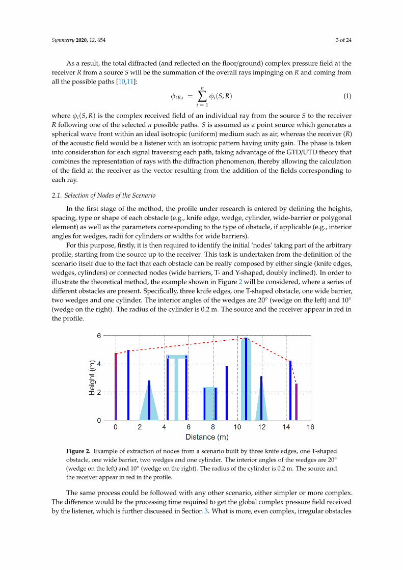
remains unobstructed with respect to the height of one intermediate obstacle, such an obstacle will bediscarded for diffraction loss calculation purposes. As a result, the radius of the Fresnel zone at anypoint P of the funicular imaginary line (red dashed line in Figure 8) in between the endpoints of anylink can be calculated as:

Rn =

√n·λ·d1·d2

d1 + d2(2)

where λ is the wavelength of the signal, n is the order of the Fresnel zone (1, 2, 3 and so on), d1 isthe distance of any point P from one end of the link and d2 is the distance of P from the other end,as shown in Figure 8. Equation (2) is derived from the application of the Huygens–Fresnel principle towave propagation analysis [13], and it characterizes the effective ellipsoid shape, with a maximumradius at the midpoint of the path.Symmetry 2020, 12, x FOR PEER REVIEW 6 of 25

Figure 7. Funicular profile created for the extracted scenario of the example in Figure 2.


Once the funicular obstacles (which are common nodes for any path) are identified, the proposed algorithm selects, for each hop that can be formed by two consecutive funicular nodes, the obstacles existing between them that are relevant in the sense of having an impact in terms of loss on the signal strength. In this respect, an obstacle is considered as relevant if it enters the Fresnel zone associated with the ray existing between the two nodes (it will block a significant percentage of energy of the transmitted signal). If the clearance of the Fresnel ellipsoid between two adjacent funicular nodes remains unobstructed with respect to the height of one intermediate obstacle, such an obstacle will be discarded for diffraction loss calculation purposes. As a result, the radius of the Fresnel zone at any point P of the funicular imaginary line (red dashed line in Figure 8) in between the endpoints of any link can be calculated as:

𝑅 = 𝑛 · λ · 𝑑 · 𝑑𝑑 + 𝑑 (2)

where λ is the wavelength of the signal, n is the order of the Fresnel zone (1, 2, 3 and so on), d1 is the distance of any point P from one end of the link and d2 is the distance of P from the other end, as shown in Figure 8. Equation (2) is derived from the application of the Huygens–Fresnel principle to wave propagation analysis [13], and it characterizes the effective ellipsoid shape, with a maximum radius at the midpoint of the path.

Figure 8. Consideration of obstacles 3, 4 and 7 within the filtered profile by applying the Fresnel zone criteria (with n = 1 and a minimum frequency of 100 Hz).

As can be seen in Figures 8 and 9 (where n = 1 and a minimum frequency of 100 Hz is considered), the obstacles 3, 4 and 7 of the example profile enter the Fresnel zone, for which they are





Once the funicular obstacles (which are common nodes for any path) are identified, the proposed algorithm selects, for each hop that can be formed by two consecutive funicular nodes, the obstacles existing between them that are relevant in the sense of having an impact in terms of loss on the signal strength. In this respect, an obstacle is considered as relevant if it enters the Fresnel zone associated with the ray existing between the two nodes (it will block a significant percentage of energy of the transmitted signal). If the clearance of the Fresnel ellipsoid between two adjacent funicular nodes remains unobstructed with respect to the height of one intermediate obstacle, such an obstacle will be discarded for diffraction loss calculation purposes. As a result, the radius of the Fresnel zone at any point P of the funicular imaginary line (red dashed line in Figure 8) in between the endpoints of any link can be calculated as:

𝑅 = 𝑛 · λ · 𝑑 · 𝑑𝑑 + 𝑑 (2)

where λ is the wavelength of the signal, n is the order of the Fresnel zone (1, 2, 3 and so on), d1 is the distance of any point P from one end of the link and d2 is the distance of P from the other end, as shown in Figure 8. Equation (2) is derived from the application of the Huygens–Fresnel principle to wave propagation analysis [13], and it characterizes the effective ellipsoid shape, with a maximum radius at the midpoint of the path.

Figure 8. Consideration of obstacles 3, 4 and 7 within the filtered profile by applying the Fresnel zone criteria (with n = 1 and a minimum frequency of 100 Hz).

As can be seen in Figures 8 and 9 (where n = 1 and a minimum frequency of 100 Hz is considered), the obstacles 3, 4 and 7 of the example profile enter the Fresnel zone, for which they are

Figure 8. Consideration of obstacles 3, 4 and 7 within the filtered profile by applying the Fresnel zonecriteria (with n = 1 and a minimum frequency of 100 Hz).

As can be seen in Figures 8 and 9 (where n = 1 and a minimum frequency of 100 Hz is considered),the obstacles 3, 4 and 7 of the example profile enter the Fresnel zone, for which they are considered asrelevant obstacles. On the contrary, the obstacles 2, 5, 6 and 9 are initially discarded, as they are out ofthe Fresnel ellipsoids for the lowest frequency of the analysis.

Since the radius of the Fresnel ellipsoid decreases with frequency, additional obstacles can beignored at higher frequencies (if the frequency band under analysis is wide). In this respect, all theclearances are firstly calculated in the proposed method in order to know the frequencies at whichobstacles can be progressively discarded depending on the radius of the corresponding Fresnel zone,

Symmetry 2020, 12, 654 7 of 24

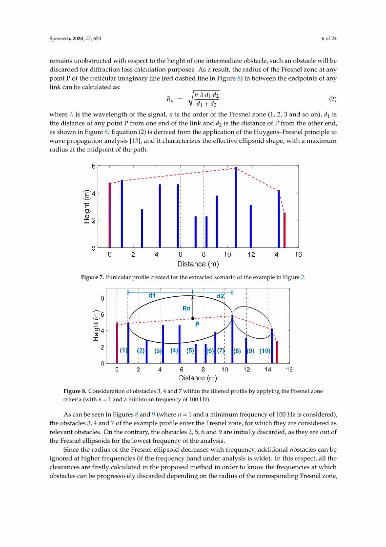
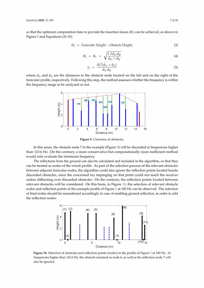
so that the optimum computation time to provide the insertion losses (IL) can be achieved, as shown inFigure 9 and Equations (3)–(5):

Hi = Funicular Height−Obstacle Heighti (3)

Hi = R1 =

√1·λd1i·d2id1i + d2i

(4)

λi =Hi

2(d1i + d2i)

d1i·d2i(5)

where d1i and d2i are the distances to the obstacle node located on the left and on the right of thefunicular profile, respectively. Following this step, the method assesses whether the frequency is withinthe frequency range to be analyzed or not.


considered as relevant obstacles. On the contrary, the obstacles 2, 5, 6 and 9 are initially discarded, as they are out of the Fresnel ellipsoids for the lowest frequency of the analysis.

Figure 9. Clearance of obstacles.

Since the radius of the Fresnel ellipsoid decreases with frequency, additional obstacles can be ignored at higher frequencies (if the frequency band under analysis is wide). In this respect, all the clearances are firstly calculated in the proposed method in order to know the frequencies at which obstacles can be progressively discarded depending on the radius of the corresponding Fresnel zone, so that the optimum computation time to provide the insertion losses (IL) can be achieved, as shown in Figure 9 and Equations (3)–(5): 𝐻 = 𝐹𝑢𝑛𝑖𝑐𝑢𝑙𝑎𝑟 𝐻𝑒𝑖𝑔ℎ𝑡 − 𝑂𝑏𝑠𝑡𝑎𝑐𝑙𝑒 𝐻𝑒𝑖𝑔ℎ𝑡 (3)

𝐻 = 𝑅 = 1 · · 𝑑 · 𝑑𝑑 + 𝑑 (4)

= 𝐻 (𝑑 + 𝑑 )𝑑 · 𝑑 (5)

where d1i and d2i are the distances to the obstacle node located on the left and on the right of the funicular profile, respectively. Following this step, the method assesses whether the frequency is within the frequency range to be analyzed or not.

In this sense, the obstacle node 7 in the example (Figure 8) will be discarded at frequencies higher than 123.6 Hz. On the contrary, a more conservative but computationally more inefficient method would only evaluate the minimum frequency.

The reflections from the ground can also be calculated and included in the algorithm, so that they can be treated as nodes of the whole profile. As part of the selection process of the relevant obstacles between adjacent funicular nodes, the algorithm could also ignore the reflection points located beside discarded obstacles, since the concerned ray impinging on that point could not reach the receiver unless diffracting over discarded obstacles. On the contrary, the reflection points located between relevant obstacles will be considered. On this basis, in Figure 10, the selection of relevant obstacle nodes and reflection points of the example profile of Figure 2 at 100 Hz can be observed. The selection of final nodes should be renumbered accordingly in case of enabling ground reflection, in order to add the reflection nodes:

Figure 9. Clearance of obstacles.

In this sense, the obstacle node 7 in the example (Figure 8) will be discarded at frequencies higherthan 123.6 Hz. On the contrary, a more conservative but computationally more inefficient methodwould only evaluate the minimum frequency.

The reflections from the ground can also be calculated and included in the algorithm, so that theycan be treated as nodes of the whole profile. As part of the selection process of the relevant obstaclesbetween adjacent funicular nodes, the algorithm could also ignore the reflection points located besidediscarded obstacles, since the concerned ray impinging on that point could not reach the receiverunless diffracting over discarded obstacles. On the contrary, the reflection points located betweenrelevant obstacles will be considered. On this basis, in Figure 10, the selection of relevant obstaclenodes and reflection points of the example profile of Figure 2 at 100 Hz can be observed. The selectionof final nodes should be renumbered accordingly in case of enabling ground reflection, in order to addthe reflection nodes:Symmetry 2020, 12, x FOR PEER REVIEW 8 of 25

Figure 10. Selection of obstacles and reflection points (nodes) in the profile of Figure 2 at 100 Hz. At frequencies higher than 123.6 Hz, the obstacle renamed as node 6, as well as the reflection node 7 will also be ignored.

2.3. Creation of Adjacency Matrix (Graph Theory)

Once the selection of the relevant obstacles and reflection points on the ground is finished, we can proceed with the next step of the method: to create the LOS matrix, that is, the adjacency matrix (A) among all the nodes of the whole profile, by using the graph definition.

We will use the terminology of graph theory [14–16], considering that we have a structure made up of vertices (V) or nodes (obstacles and reflection points), which are connected through the edges, E (set of LOS links), building the graph input variables G (V, E).

Specifically, we obtain a so-called directed graph or digraph, that is, without loops (a tree), because the edges link two vertices asymmetrically (the rays will not return to previous edges). In this respect, we neglect the paths from rays diffracted twice or more by the same edge, as could happen in obstacles with connected edges, such as wide barriers.

An upper triangular square matrix of 1s (when LOS exists between node u and node v, A[u][v] = 1) and 0s (otherwise) is then obtained for the adjacency matrix (|V| x |V|) with the main diagonal filled with zeros and order V, with V being the total number of selected nodes of the scenario.

A general overview of the digraphs created by these profiles is shown in Figure 11, with the particularity that all paths must go through the funicular nodes (Fi).

Figure 11. General line of sight (LOS) path directed graph (digraph). Funicular nodes (Fi), in red, including source and receiver, are common nodes for any path.

The graph obtained from the adjacency matrix of the final profile of the example of Figure 10, including ground reflection nodes, can be seen in Figure 12, where the funicular nodes are 1, 3, 8, 9 and 11:

Hei

ght (

m)

p l F1

F2 F3

Fn j

i

k m o

Figure 10. Selection of obstacles and reflection points (nodes) in the profile of Figure 2 at 100 Hz. Atfrequencies higher than 123.6 Hz, the obstacle renamed as node 6, as well as the reflection node 7 willalso be ignored.

Symmetry 2020, 12, 654 8 of 24


Once the selection of the relevant obstacles and reflection points on the ground is finished, we canproceed with the next step of the method: to create the LOS matrix, that is, the adjacency matrix (A)among all the nodes of the whole profile, by using the graph definition.

We will use the terminology of graph theory [14–16], considering that we have a structure madeup of vertices (V) or nodes (obstacles and reflection points), which are connected through the edges, E(set of LOS links), building the graph input variables G (V, E).

Specifically, we obtain a so-called directed graph or digraph, that is, without loops (a tree), becausethe edges link two vertices asymmetrically (the rays will not return to previous edges). In this respect,we neglect the paths from rays diffracted twice or more by the same edge, as could happen in obstacleswith connected edges, such as wide barriers.

An upper triangular square matrix of 1s (when LOS exists between node u and node v, A[u][v] = 1)and 0s (otherwise) is then obtained for the adjacency matrix (|V| x |V|) with the main diagonal filledwith zeros and order V, with V being the total number of selected nodes of the scenario.

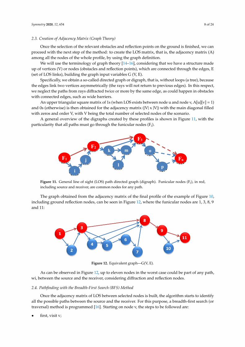
A general overview of the digraphs created by these profiles is shown in Figure 11, with theparticularity that all paths must go through the funicular nodes (Fi).


Figure 10. Selection of obstacles and reflection points (nodes) in the profile of Figure 2 at 100 Hz. At frequencies higher than 123.6 Hz, the obstacle renamed as node 6, as well as the reflection node 7 will also be ignored.


Once the selection of the relevant obstacles and reflection points on the ground is finished, we can proceed with the next step of the method: to create the LOS matrix, that is, the adjacency matrix (A) among all the nodes of the whole profile, by using the graph definition.

We will use the terminology of graph theory [14–16], considering that we have a structure made up of vertices (V) or nodes (obstacles and reflection points), which are connected through the edges, E (set of LOS links), building the graph input variables G (V, E).

Specifically, we obtain a so-called directed graph or digraph, that is, without loops (a tree), because the edges link two vertices asymmetrically (the rays will not return to previous edges). In this respect, we neglect the paths from rays diffracted twice or more by the same edge, as could happen in obstacles with connected edges, such as wide barriers.

An upper triangular square matrix of 1s (when LOS exists between node u and node v, A[u][v] = 1) and 0s (otherwise) is then obtained for the adjacency matrix (|V| x |V|) with the main diagonal filled with zeros and order V, with V being the total number of selected nodes of the scenario.

A general overview of the digraphs created by these profiles is shown in Figure 11, with the particularity that all paths must go through the funicular nodes (Fi).

Figure 11. General line of sight (LOS) path directed graph (digraph). Funicular nodes (Fi), in red, including source and receiver, are common nodes for any path.

The graph obtained from the adjacency matrix of the final profile of the example of Figure 10, including ground reflection nodes, can be seen in Figure 12, where the funicular nodes are 1, 3, 8, 9 and 11:

Hei

ght (

m)

p l F1

F2 F3

Fn j

i

k m o

Figure 11. General line of sight (LOS) path directed graph (digraph). Funicular nodes (Fi), in red,including source and receiver, are common nodes for any path.

The graph obtained from the adjacency matrix of the final profile of the example of Figure 10,including ground reflection nodes, can be seen in Figure 12, where the funicular nodes are 1, 3, 8, 9and 11:Symmetry 2020, 12, x FOR PEER REVIEW 9 of 25

Figure 12. Equivalent graph—G(V, E).

As can be observed in Figure 12, up to eleven nodes in the worst case could be part of any path, wi, between the source and the receiver, considering diffraction and reflection nodes.

2.4. Pathfinding with the Breadth-First Search (BFS) Method

Once the adjacency matrix of LOS between selected nodes is built, the algorithm starts to identify all the possible paths between the source and the receiver. For this purpose, a breadth-first search (or traversal) method is programmed [16]. Starting on node v, the steps to be followed are: • first, visit v; • then, all its adjacent vertices are visited; • next, those adjacent to the latter are visited, and so on.

The maximum number of possible paths between the source and the receiver can be easily determined in advance by [16]:

𝑃𝑎𝑡ℎ𝑠 = 𝐴 1 𝑉 (6)

Therefore, the total feasible paths for the previous example, once properly filtered (Figure 12), would be 32.

The adjacency matrix, as well as the pathfinding, will be carried out again in each Fresnel frequency sub-band, so that the process of calculating the final sound pressure level will be significantly accelerated, since the number of nodes and paths will also appreciably decrease.

The importance of the process of selecting relevant nodes according to its influence in the final sound pressure field can be better understood if the same process is carried out without discarding any obstacle. In such a case, in the example of Figure 2, the total nodes (including reflections) would sum up 21 nodes, which would increase the number of possible paths of the equivalent graph up to 2291.

Moreover, it is also paramount to constrain the maximum number of hops or links when searching the possible paths from the source to the receiver, especially when the total amount of nodes of the final scenario is high. For this reason, the software code developed allows us to also manually or automatically tune this parameter.

2.5. Calculation of Total Sound Pressure Field at the Receiver

Following the previous task, the path matrix is now properly rearranged and sorted from the shortest path to the longest one, according to their number of nodes.

A loop then runs each frequency bin, from the minimum to the maximum, to provide the total sound pressure field for the complete set of paths for such a frequency. For each frequency, the algorithm also allows us to check the sound pressure field level at the receiver for each path. As the set of paths is sorted, it is expected that the subsequent sub-fields will be progressively decreasing, so that an adjustable threshold condition is defined in order to interrupt the addition of new fields if the current field is below the threshold. Such a threshold can be defined as the absolute value of the ratio between the level of signal received for the shortest path at such a frequency and the level of

Figure 12. Equivalent graph—G(V, E).

As can be observed in Figure 12, up to eleven nodes in the worst case could be part of any path,wi, between the source and the receiver, considering diffraction and reflection nodes.

2.4. Pathfinding with the Breadth-First Search (BFS) Method

Once the adjacency matrix of LOS between selected nodes is built, the algorithm starts to identifyall the possible paths between the source and the receiver. For this purpose, a breadth-first search (ortraversal) method is programmed [16]. Starting on node v, the steps to be followed are:

• first, visit v;

Symmetry 2020, 12, 654 9 of 24

• then, all its adjacent vertices are visited;• next, those adjacent to the latter are visited, and so on.

The maximum number of possible paths between the source and the receiver can be easilydetermined in advance by [16]:

Paths =V∑

i = 1

Ai[1][V] (6)

Therefore, the total feasible paths for the previous example, once properly filtered (Figure 12),would be 32.

The adjacency matrix, as well as the pathfinding, will be carried out again in each Fresnelfrequency sub-band, so that the process of calculating the final sound pressure level will be significantlyaccelerated, since the number of nodes and paths will also appreciably decrease.

The importance of the process of selecting relevant nodes according to its influence in the finalsound pressure field can be better understood if the same process is carried out without discarding anyobstacle. In such a case, in the example of Figure 2, the total nodes (including reflections) would sumup 21 nodes, which would increase the number of possible paths of the equivalent graph up to 2291.

Moreover, it is also paramount to constrain the maximum number of hops or links when searchingthe possible paths from the source to the receiver, especially when the total amount of nodes of thefinal scenario is high. For this reason, the software code developed allows us to also manually orautomatically tune this parameter.

2.5. Calculation of Total Sound Pressure Field at the Receiver

Following the previous task, the path matrix is now properly rearranged and sorted from theshortest path to the longest one, according to their number of nodes.

A loop then runs each frequency bin, from the minimum to the maximum, to provide the totalsound pressure field for the complete set of paths for such a frequency. For each frequency, thealgorithm also allows us to check the sound pressure field level at the receiver for each path. As theset of paths is sorted, it is expected that the subsequent sub-fields will be progressively decreasing,so that an adjustable threshold condition is defined in order to interrupt the addition of new fields ifthe current field is below the threshold. Such a threshold can be defined as the absolute value of theratio between the level of signal received for the shortest path at such a frequency and the level ofsignal received for the current path (e.g., 1 × 10−4). Therefore, a threshold level of 0 would imply notdiscarding any path.

It should be noted that the computational time of the proposed algorithm is frequency-independentwhen the threshold is set to 0 and can always be limited or restrained, since the worst case can beforeseen in advance just by multiplying the consumed time at any frequency by the number of frequencybins considered in the simulation.

Regarding the above, the expression to obtain the complex field at the receiver, for each path i andeach frequency is:

φtpath i =φ0

sT·e− jksT ·

N−2∏n = 1

(Dn

Rn

)·

√sT∏N−1

i = 1(sk)·γ (7)

where:φ0 is the sound pressure level transmitted by the source;sT =

∑Ni = 1 si, with si being the slant distances of the links of the selected paths, between the

geometrical centers of each node;N is the number of nodes of each path;k is the wavenumber;Dn and Rn are the diffraction or reflection coefficients, respectively, applied depending on the type

of incidence to either the obstacles or the ground;

Symmetry 2020, 12, 654 10 of 24

γ is the obstacle coefficient factor. This expression comes from [10] and [11] but including, in thiscase, the γ coefficient factor with two purposes: to adjust the phase, and as a weight factor ([3,6]), foreach kind of obstacle considered in the present work.

The total sound pressure at the receiver for each frequency bin will be the summation of all thesound pressure signals for all the selected paths arriving to the receiver, as shown in Equation (1).

It should be noted that the e+iωt time-dependence term has been implicitly assumed and suppressedthroughout the present study.

Next, the different coefficients considered in Equation (7) will be properly explained.

2.5.1. Obstacle Coefficient Factor γ

By means of the γ factor, the general expression in Equation (7) considers the specific modificationsof the amplitude (spreading factors) to be applied depending on the type of obstacles, diffractions orreflections for the path under analysis. Otherwise, such an expression would only be applicable forknife edges and wedges. At the beginning of each path iteration, γ is reset to 1 and is progressivelyadjusted when considering either reflections on the ground or diffractions over obstacles between thetwo ends of the path:

• γ(n) = γ(n− 1)·γR, ground reflection case, where n is the index of the current obstacle of thepath, with

γR =AR

AD, AR =

sisi+1 + si

, AD =

√si

si+1·(si + si+1)(8)

• γ(n) = γ(n− 1)·γb, diffraction over wide barriers case, with [6]

γb =

1, i f the edges o f the obstacleand the receiver are not connected

0.5, i f the edges o f the obstacleand the receive are connected

(9)

• γ(n) = γ(n− 1)·γc, diffraction over cylinders case, with

γc =

1, LOS between Tx and Rx, lit region

AD1AD2·e−ik(ta+ssi+1−si+1)

e−ik(si−ssi), shadow region

(10)

With

AD1 =

√ssi

ssi+1·(ssi + ssi+1)(11)

AD2 =

√si

si+1·(si + si+1)(12)

where:

ssi is the distance of the incident ray impinging on the cylinder;ssi+1 is the distance of the diffracted ray from the cylinder to the next end;and ta is the arc length traveled by the creeping wave over the cylinder from the incidence point to theexit one.

Symmetry 2020, 12, 654 11 of 24

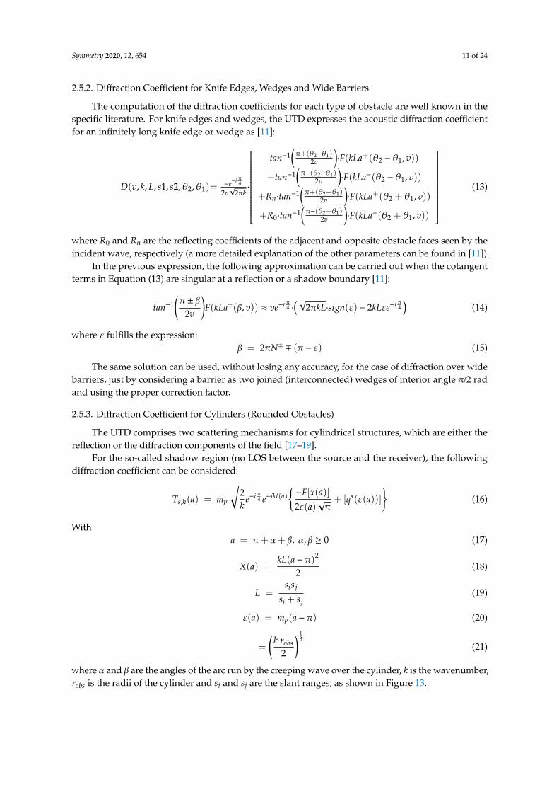
2.5.2. Diffraction Coefficient for Knife Edges, Wedges and Wide Barriers

The computation of the diffraction coefficients for each type of obstacle are well known in thespecific literature. For knife edges and wedges, the UTD expresses the acoustic diffraction coefficientfor an infinitely long knife edge or wedge as [11]:

D(v, k, L, s1, s2,θ2,θ1)=−e−i π4

2v√

2πk·

tan−1(π+(θ2−θ1)

2v

)·F(kLa+(θ2 − θ1, v))

+tan−1(π−(θ2−θ1)

2v

)·F(kLa−(θ2 − θ1, v))

+Rn·tan−1(π+(θ2+θ1)

2v

)·F(kLa+(θ2 + θ1, v))

+R0·tan−1(π−(θ2+θ1)

2v

)·F(kLa−(θ2 + θ1, v))

(13)

where R0 and Rn are the reflecting coefficients of the adjacent and opposite obstacle faces seen by theincident wave, respectively (a more detailed explanation of the other parameters can be found in [11]).

In the previous expression, the following approximation can be carried out when the cotangentterms in Equation (13) are singular at a reflection or a shadow boundary [11]:

tan−1(π± β

2v

)F(kLa±(β, v)) ≈ ve−i π4 ·

(√2πkL·sign(ε) − 2kLεe−i π4

)(14)

where ε fulfills the expression:β = 2πN± ∓ (π− ε) (15)

The same solution can be used, without losing any accuracy, for the case of diffraction over widebarriers, just by considering a barrier as two joined (interconnected) wedges of interior angle π/2 radand using the proper correction factor.

2.5.3. Diffraction Coefficient for Cylinders (Rounded Obstacles)

The UTD comprises two scattering mechanisms for cylindrical structures, which are either thereflection or the diffraction components of the field [17–19].

For the so-called shadow region (no LOS between the source and the receiver), the followingdiffraction coefficient can be considered:

Ts,h(a) = mp

√2k

e−i π4 e−ikt(a){−F[x(a)]2ε(a)

√π+ [q∗(ε(a))]

}(16)

Witha = π+ α+ β, α, β ≥ 0 (17)

X(a) =kL(a−π)2

2(18)

L =sis j

si + s j(19)

ε(a) = mp(a−π) (20)

=

(k·robs

2

) 13

(21)

where α and β are the angles of the arc run by the creeping wave over the cylinder, k is the wavenumber,robs is the radii of the cylinder and si and sj are the slant ranges, as shown in Figure 13.

Symmetry 2020, 12, 654 12 of 24


For the so-called shadow region (no LOS between the source and the receiver), the following diffraction coefficient can be considered:

𝑇 , (𝑎) = 𝑚 2𝑘 𝑒 𝑒 ( ) −𝐹 𝑥(𝑎)2𝜀(𝑎)√𝜋 + 𝑞∗ 𝜀(𝑎) (16)

With 𝑎 = 𝜋 + 𝛼 + 𝛽, 𝛼, 𝛽 ≥ 0 (17) 𝑋(𝑎) = 𝑘𝐿(𝑎 − 𝜋)2 (18)

𝐿 = 𝑠 𝑠𝑠 + 𝑠 (19) 𝜀(𝑎) = 𝑚 (𝑎 − 𝜋) (20)

= 𝑘 · 𝑟2 (21)

where α and β are the angles of the arc run by the creeping wave over the cylinder, k is the wavenumber, 𝑟 is the radii of the cylinder and si and sj are the slant ranges, as shown in Figure 13.

Figure 13. Parameters considered for the obstacle with a cylindrical shape for the shadow region.

The first addend of Equation (16) describes the Fresnel diffraction process. F[x] is the so-called transition function, which is defined in terms of a Fresnel integral [11]: 𝐹 𝑥 = 2𝑖√𝑥𝑒 𝑒 𝑑𝑢√ (22)

In the second addend of Equation (16), the term q*(ε(a)) is the so-called Fock scattering function, and addresses the generation of creeping waves along the surface of a smooth body, such as spheres or cylinders [17]: 𝑞∗(𝑥) = 12√𝜋𝑥 + 1√𝜋 𝑉 ( )𝑤 (𝑡) 𝑒 𝑑𝑡 (23)

(the prime represents differentiation with respect to argument), where V(t) and w2 (t) are defined as: 𝑉(𝑡) = √𝜋𝐴 (𝑡) (24) 𝑤 = 2√𝜋𝑒 𝐴 𝑡𝑒 (25)

with Ai(t) as a Miller-type Airy function:

Figure 13. Parameters considered for the obstacle with a cylindrical shape for the shadow region.

The first addend of Equation (16) describes the Fresnel diffraction process. F[x] is the so-calledtransition function, which is defined in terms of a Fresnel integral [11]:

F[x] = 2i√

xeix∫∞

√x

e−iu2du (22)

In the second addend of Equation (16), the term q*(ε(a)) is the so-called Fock scattering function,and addresses the generation of creeping waves along the surface of a smooth body, such as spheres orcylinders [17]:

q∗(x) =1

2√πx

+1√π

∫∞

−∞

V′(t)

w′2(t)e−ixtdt (23)

(the prime represents differentiation with respect to argument), where V(t) and w2(t) are defined as:

V(t) =√πAi(t) (24)

w2 = 2√πe−i π6 Ai

(te−i 2π

3

)(25)

with Ai(t) as a Miller-type Airy function:

Ai(t) =1π

∫∞

0cos

(13

zs + tz)dz (26)

For the so-called lit region (LOS between the source and the receiver), the following diffractioncoefficient is applicable instead:

Rs,h(a) =

√r

m′e−i ε

3(a)12 e−i π4

{−F[x(a)]2ε(a)

√π+ [q∗(ε(a))]

}(27)

where a is again the angle between the incident and the diffracted ray, as given in Figure 14, and:

ε(a) = −2mp

(cos

( a2

))(28)

Xa = 2kL(cos

( a2

))2(29)

with L as in Equation (19).

Symmetry 2020, 12, 654 13 of 24


𝐴 (𝑡) = 1𝜋 𝑐𝑜𝑠 13 𝑧𝑠 + 𝑡𝑧 𝑑𝑧 (26)

For the so-called lit region (LOS between the source and the receiver), the following diffraction coefficient is applicable instead: 𝑅 , (𝑎) = 𝑟𝑚 𝑒 ( )𝑒 −𝐹 𝑥(𝑎)2𝜀(𝑎)√𝜋 + 𝑞∗ 𝜀(𝑎) (27)

where a is again the angle between the incident and the diffracted ray, as given in Figure 14, and:

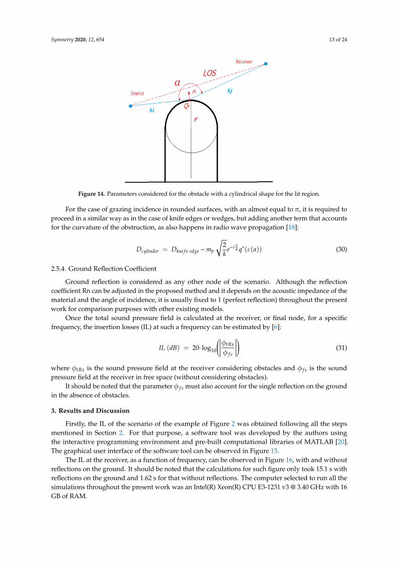
Figure 14. Parameters considered for the obstacle with a cylindrical shape for the lit region.

𝜀(𝑎) = −2𝑚 cos 𝑎2 (28)

𝑋 = 2𝑘𝐿 cos 𝑎2 (29)

with L as in Equation (19). For the case of grazing incidence in rounded surfaces, with an almost equal to π, it is required

to proceed in a similar way as in the case of knife edges or wedges, but adding another term that accounts for the curvature of the obstruction, as also happens in radio wave propagation [18]:

𝐷 = 𝐷 − 𝑚 2𝑘 𝑒 𝑞∗ 𝜀(𝑎) (30)

2.5.4. Ground Reflection Coefficient

Ground reflection is considered as any other node of the scenario. Although the reflection coefficient Rn can be adjusted in the proposed method and it depends on the acoustic impedance of the material and the angle of incidence, it is usually fixed to 1 (perfect reflection) throughout the present work for comparison purposes with other existing models.

Once the total sound pressure field is calculated at the receiver, or final node, for a specific frequency, the insertion losses (IL) at such a frequency can be estimated by [6]: 𝐼𝐿 (𝑑𝐵) = 20 · log 𝜙𝜙 (31)

Figure 14. Parameters considered for the obstacle with a cylindrical shape for the lit region.

For the case of grazing incidence in rounded surfaces, with an almost equal to π, it is required toproceed in a similar way as in the case of knife edges or wedges, but adding another term that accountsfor the curvature of the obstruction, as also happens in radio wave propagation [18]:

Dcylinder = Dkni f e edge −mp

√2k

e−i π4 q∗(ε(a)) (30)

2.5.4. Ground Reflection Coefficient

Ground reflection is considered as any other node of the scenario. Although the reflectioncoefficient Rn can be adjusted in the proposed method and it depends on the acoustic impedance of thematerial and the angle of incidence, it is usually fixed to 1 (perfect reflection) throughout the presentwork for comparison purposes with other existing models.

Once the total sound pressure field is calculated at the receiver, or final node, for a specificfrequency, the insertion losses (IL) at such a frequency can be estimated by [6]:

IL (dB) = 20· log10

(∣∣∣∣∣∣φtRx

φ f s

∣∣∣∣∣∣)

(31)

where φtRx is the sound pressure field at the receiver considering obstacles and φ f s is the soundpressure field at the receiver in free space (without considering obstacles).

It should be noted that the parameter φ f s must also account for the single reflection on the groundin the absence of obstacles.

3. Results and Discussion

Firstly, the IL of the scenario of the example of Figure 2 was obtained following all the stepsmentioned in Section 2. For that purpose, a software tool was developed by the authors usingthe interactive programming environment and pre-built computational libraries of MATLAB [20].The graphical user interface of the software tool can be observed in Figure 15.

The IL at the receiver, as a function of frequency, can be observed in Figure 16, with and withoutreflections on the ground. It should be noted that the calculations for such figure only took 15.1 s withreflections on the ground and 1.62 s for that without reflections. The computer selected to run all thesimulations throughout the present work was an Intel(R) Xeon(R) CPU E3-1231 v3 @ 3.40 GHz with 16GB of RAM.

Symmetry 2020, 12, 654 14 of 24

It should be noted that, in spite of ignoring the obstacle node 7 of Figure 8 from 123.6 Hz andobstacle nodes 3 and 4 from 1777.6 Hz onwards (due to the fact that the radius of the Fresnel zonedecreases with frequency), the IL curve in the results of Figure 16 continued its increasing behavior upto 2000 Hz due to the fact that the diffraction coefficient also decreases with frequency.


where 𝜙 is the sound pressure field at the receiver considering obstacles and φ is the sound pressure field at the receiver in free space (without considering obstacles).

It should be noted that the parameter 𝜙 must also account for the single reflection on the ground in the absence of obstacles.


Firstly, the IL of the scenario of the example of Figure 2 was obtained following all the steps mentioned in section 2. For that purpose, a software tool was developed by the authors using the interactive programming environment and pre-built computational libraries of MATLAB [20]. The graphical user interface of the software tool can be observed in Figure 15.

Figure 15. Graphical user interface of the software tool. Scenario of Figure 2 created on the right display.

The IL at the receiver, as a function of frequency, can be observed in Figure 16, with and without reflections on the ground. It should be noted that the calculations for such figure only took 15.1 s with reflections on the ground and 1.62 s for that without reflections. The computer selected to run all the simulations throughout the present work was an Intel(R) Xeon(R) CPU E3-1231 v3 @ 3.40 GHz with 16 GB of RAM.

Figure 16. IL (dB) of the scenario of the example of Figure 2, with (red line) and without (black line) reflections on the ground.

Inse

rtion

Los

ses

(dB)



where 𝜙 is the sound pressure field at the receiver considering obstacles and φ is the sound pressure field at the receiver in free space (without considering obstacles).

It should be noted that the parameter 𝜙 must also account for the single reflection on the ground in the absence of obstacles.


Firstly, the IL of the scenario of the example of Figure 2 was obtained following all the steps mentioned in section 2. For that purpose, a software tool was developed by the authors using the interactive programming environment and pre-built computational libraries of MATLAB [20]. The graphical user interface of the software tool can be observed in Figure 15.


The IL at the receiver, as a function of frequency, can be observed in Figure 16, with and without reflections on the ground. It should be noted that the calculations for such figure only took 15.1 s with reflections on the ground and 1.62 s for that without reflections. The computer selected to run all the simulations throughout the present work was an Intel(R) Xeon(R) CPU E3-1231 v3 @ 3.40 GHz with 16 GB of RAM.

Figure 16. IL (dB) of the scenario of the example of Figure 2, with (red line) and without (black line) reflections on the ground.

Inse

rtion

Los

ses

(dB)

Figure 16. IL (dB) of the scenario of the example of Figure 2, with (red line) and without (black line)reflections on the ground.

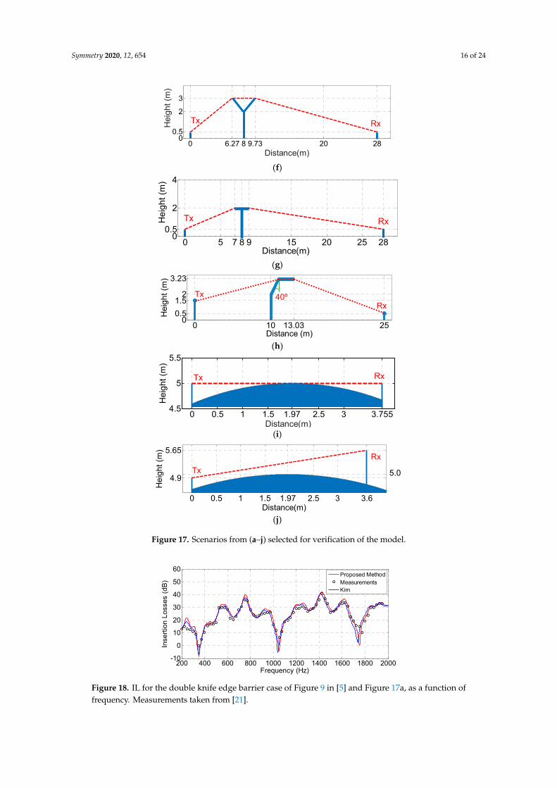
The proposed method was properly compared with other validated formulations published byother authors, considering different scenarios (including different types of obstacles), in order to verifyits accuracy. In Figure 17, the different scenarios considered for the validation of the proposed modelare shown.

Firstly, in Figures 18 and 19, the IL as a function of frequency are compared with the IL providedby Kim et al. [5] (scenarios and parameters taken from Figures 4 and 9 of [5], respectively) for a doubleknife edge case (Figure 17a) and a double wedge case (Figure 17b). In Figure 18, the measurement datataken from [21] are also depicted for comparison.

As can be observed, good agreement is obtained between the proposed method and the formulationpresented in [5] in both cases, taking our solution simulation times of only 1.27 and 0.94 s inFigures 18 and 19, respectively, for the obtaining of the IL in the whole frequency range (with 1500frequency bins). Moreover, the agreement of the results obtained with the proposed method with themeasurements in Figure 18 seems to be better in some frequencies—especially in the valleys of thecurve—than those achieved by Kim et al.

Symmetry 2020, 12, 654 15 of 24


It should be noted that, in spite of ignoring the obstacle node 7 of Figure 8 from 123.6 Hz and obstacle nodes 3 and 4 from 1777.6 Hz onwards (due to the fact that the radius of the Fresnel zone decreases with frequency), the IL curve in the results of Figure 16 continued its increasing behavior up to 2000 Hz due to the fact that the diffraction coefficient also decreases with frequency.

The proposed method was properly compared with other validated formulations published by other authors, considering different scenarios (including different types of obstacles), in order to verify its accuracy. In Figure 17, the different scenarios considered for the validation of the proposed model are shown.

(a)

(b)

(c)

(d)

(e)

0 5 10 13 14.5 180

0.51

2

3

Distance(m)H

eigh

t (m

)

RxTx

0 5 10 13 14.5 180

0.51

2

3

Distance(m)

Hei

ght (

m)

RxTx

0 2 3.2 3.8 4.8 5.4 8.340

0.41

22.4

Distance(m)

Hei

ght (

m)

0.5Tx Rx

0 1 2 3.2 3.8 4.8 5.4 6.4 70

1

2.43

Distance(m)

Hei

ght (

m)

2.9Rx

Tx

7.17

0 2 3.2 3.8 4.8 5.4 6.4 7 9.4500.4

1

22.4

3

Distance(m)

Hei

ght (

m)

Tx Rx0.5

Figure 17. Cont.

Symmetry 2020, 12, 654 16 of 24Symmetry 2020, 12, x FOR PEER REVIEW 16 of 25

(f)

(g)

(h)

(i)

(j)

Figure 17. Scenarios from (a) to (j) selected for verification of the model.

Firstly, in Figures 18 and 19, the IL as a function of frequency are compared with the IL provided by Kim et al. [5] (scenarios and parameters taken from Figures 4 and 9 of [5], respectively) for a double knife edge case (Figure 17a) and a double wedge case (Figure 17b). In Figure 18, the measurement data taken from [21] are also depicted for comparison.

0 6.27 8 9.73 20 280

0.5

2

3

Distance(m)H

eigh

t (m

)

RxTx

0 5 7 8 9 15 20 25 280

0.5

2

4

Distance(m)

Hei

ght (

m)

RxTx

0 10 13.03 2500.51.5

2

3.23

Distance (m)

Hei

ght (

m)

TxRx

40º

0 0.5 1 1.5 1.97 2.5 3 3.7554.5

5

5.5

Distance(m)

Hei

ght (

m)

Tx Rx

0 0.5 1 1.5 1.97 2.5 3 3.6

4.9

5.65

Distance(m)

Hei

ght (

m)

TxRx

5.0

Figure 17. Scenarios from (a–j) selected for verification of the model.Symmetry 2020, 12, x FOR PEER REVIEW 17 of 25

Figure 18. IL for the double knife edge barrier case of Figure 9 in [5] and Figure 17a, as a function of frequency. Measurements taken from [21].

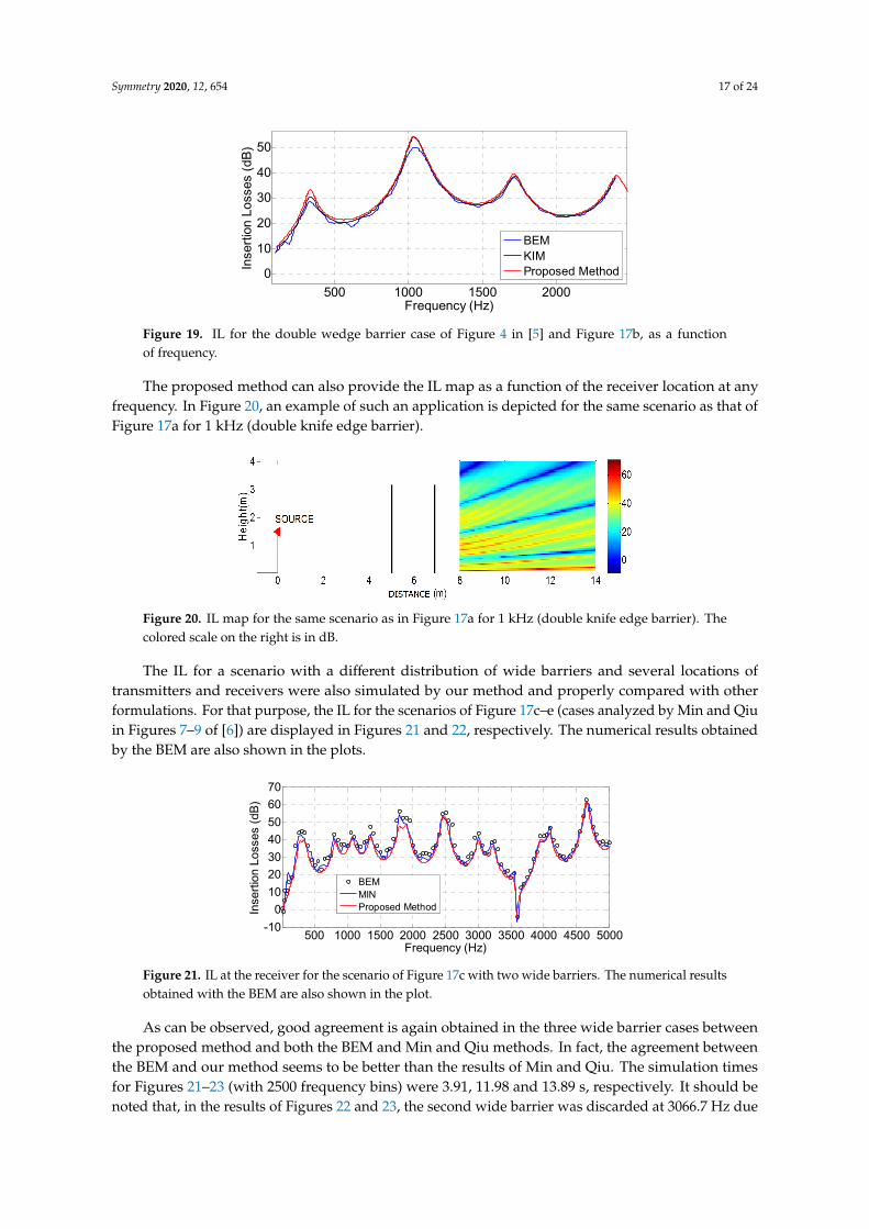
Figure 19. IL for the double wedge barrier case of Figure 4 in [5] and Figure 17b, as a function of frequency.

As can be observed, good agreement is obtained between the proposed method and the formulation presented in [5] in both cases, taking our solution simulation times of only 1.27 and 0.94 s in Figures 18 and 19, respectively, for the obtaining of the IL in the whole frequency range (with 1500 frequency bins). Moreover, the agreement of the results obtained with the proposed method with the measurements in Figure 18 seems to be better in some frequencies—especially in the valleys of the curve—than those achieved by Kim et al.

The proposed method can also provide the IL map as a function of the receiver location at any frequency. In Figure 20, an example of such an application is depicted for the same scenario as that of Figure 17a for 1 kHz (double knife edge barrier).

Figure 20. IL map for the same scenario as in Figure 17a for 1 kHz (double knife edge barrier). The colored scale on the right is in dB.

The IL for a scenario with a different distribution of wide barriers and several locations of transmitters and receivers were also simulated by our method and properly compared with other formulations. For that purpose, the IL for the scenarios of Figure 17c–e (cases analyzed by Min and Qiu in Figures 7–9 of [6]) are displayed in Figures 21 and 22, respectively. The numerical results obtained by the BEM are also shown in the plots.

200 400 600 800 1000 1200 1400 1600 1800 2000-10

0

10

20

30

40

50

60

Frequency (Hz)

Inse

rtion

Los

ses

(dB)

Proposed MethodMeasurementsKim

500 1000 1500 20000

10

20

30

40

50

Frequency (Hz)

Inse

rtion

Los

ses

(dB)

BEMKIMProposed Method

Figure 18. IL for the double knife edge barrier case of Figure 9 in [5] and Figure 17a, as a function offrequency. Measurements taken from [21].

Symmetry 2020, 12, 654 17 of 24








200 400 600 800 1000 1200 1400 1600 1800 2000-10

0

10

20

30

40

50

60

Frequency (Hz)

Inse

rtion

Los

ses

(dB)


500 1000 1500 20000

10

20

30

40

50

Frequency (Hz)

Inse

rtion

Los

ses

(dB)


Figure 19. IL for the double wedge barrier case of Figure 4 in [5] and Figure 17b, as a functionof frequency.

The proposed method can also provide the IL map as a function of the receiver location at anyfrequency. In Figure 20, an example of such an application is depicted for the same scenario as that ofFigure 17a for 1 kHz (double knife edge barrier).








200 400 600 800 1000 1200 1400 1600 1800 2000-10

0

10

20

30

40

50

60

Frequency (Hz)

Inse

rtion

Los

ses

(dB)


500 1000 1500 20000

10

20

30

40

50

Frequency (Hz)

Inse

rtion

Los

ses

(dB)


Figure 20. IL map for the same scenario as in Figure 17a for 1 kHz (double knife edge barrier). Thecolored scale on the right is in dB.

The IL for a scenario with a different distribution of wide barriers and several locations oftransmitters and receivers were also simulated by our method and properly compared with otherformulations. For that purpose, the IL for the scenarios of Figure 17c–e (cases analyzed by Min and Qiuin Figures 7–9 of [6]) are displayed in Figures 21 and 22, respectively. The numerical results obtainedby the BEM are also shown in the plots.Symmetry 2020, 12, x FOR PEER REVIEW 18 of 25

Figure 21. IL at the receiver for the scenario of Figure 17c with two wide barriers. The numerical results obtained with the BEM are also shown in the plot.

Figure 22. IL at the receiver for the scenario of Figure 17d with three wide barriers. The numerical results obtained with the BEM are also shown in the plot.

As can be observed, good agreement is again obtained in the three wide barrier cases between the proposed method and both the BEM and Min and Qiu methods. In fact, the agreement between the BEM and our method seems to be better than the results of Min and Qiu. The simulation times for Figures 21–23 (with 2500 frequency bins) were 3.91, 11.98 and 13.89 s, respectively. It should be noted that, in the results of Figures 22 and 23, the second wide barrier was discarded at 3066.7 Hz due to the decrease of the radius of the Fresnel zone with frequency, as previously mentioned, with the consequent reduction in terms of computational time.

Figure 23. IL at the receiver for the scenario of Figure 17e with three wide barriers. The numerical results obtained with the BEM are also shown in the plot.

Following the comparison of the results obtained with knife edges, wedges and wide barriers, additional simulations of the expected IL for doubly inclined, Y- and T-shaped barriers were undertaken. Figures 24–26 present the simulations for the scenarios depicted in Figure 17f–h (from Figures 13, 15 and 17 of [5]), respectively. The numerical results obtained by the BEM are also shown in the plots.

500 1000 1500 2000 2500 3000 3500 4000 4500 5000-10

010203040506070

Frequency (Hz)

Inse

rtion

Los

ses

(dB)

BEMMINProposed Method

0 1000 2000 3000 4000 5000-10

01020304050

Frequency (Hz)

Inse

rtion

Los

ses

(dB)

Proposed MethodBEMMIN

0 1000 2000 3000 4000 50000

20

40

60

80

Frequency (Hz)

Inse

rtion

Los

ses

(dB)


Figure 21. IL at the receiver for the scenario of Figure 17c with two wide barriers. The numerical resultsobtained with the BEM are also shown in the plot.

As can be observed, good agreement is again obtained in the three wide barrier cases betweenthe proposed method and both the BEM and Min and Qiu methods. In fact, the agreement betweenthe BEM and our method seems to be better than the results of Min and Qiu. The simulation timesfor Figures 21–23 (with 2500 frequency bins) were 3.91, 11.98 and 13.89 s, respectively. It should benoted that, in the results of Figures 22 and 23, the second wide barrier was discarded at 3066.7 Hz due

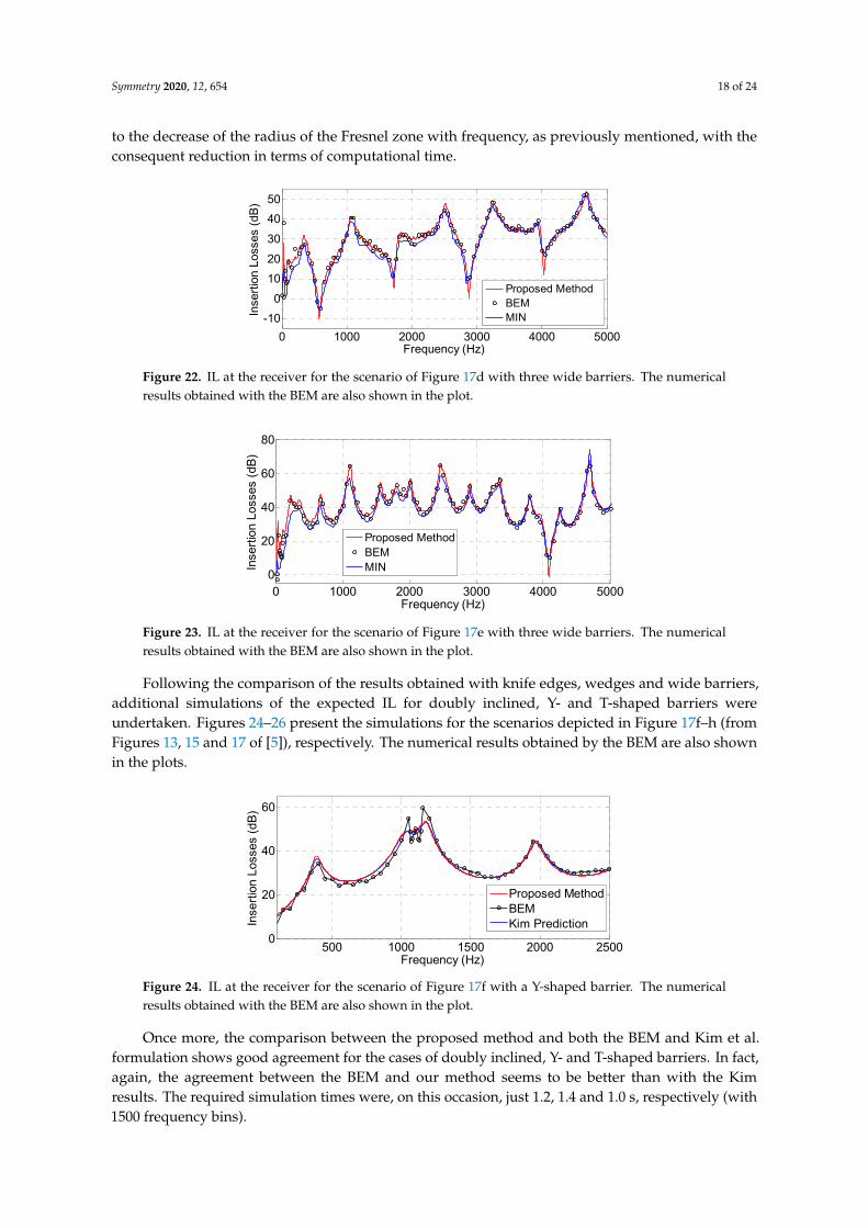
Symmetry 2020, 12, 654 18 of 24

to the decrease of the radius of the Fresnel zone with frequency, as previously mentioned, with theconsequent reduction in terms of computational time.







500 1000 1500 2000 2500 3000 3500 4000 4500 5000-10

010203040506070

Frequency (Hz)

Inse

rtion

Los

ses

(dB)


0 1000 2000 3000 4000 5000-10

01020304050

Frequency (Hz)

Inse

rtion

Los

ses

(dB)


0 1000 2000 3000 4000 50000

20

40

60

80

Frequency (Hz)

Inse

rtion

Los

ses

(dB)


Figure 22. IL at the receiver for the scenario of Figure 17d with three wide barriers. The numericalresults obtained with the BEM are also shown in the plot.







500 1000 1500 2000 2500 3000 3500 4000 4500 5000-10

010203040506070

Frequency (Hz)

Inse

rtion

Los

ses

(dB)


0 1000 2000 3000 4000 5000-10

01020304050

Frequency (Hz)

Inse

rtion

Los

ses

(dB)


0 1000 2000 3000 4000 50000

20

40

60

80

Frequency (Hz)

Inse

rtion

Los

ses

(dB)


Figure 23. IL at the receiver for the scenario of Figure 17e with three wide barriers. The numericalresults obtained with the BEM are also shown in the plot.

Following the comparison of the results obtained with knife edges, wedges and wide barriers,additional simulations of the expected IL for doubly inclined, Y- and T-shaped barriers wereundertaken. Figures 24–26 present the simulations for the scenarios depicted in Figure 17f–h (fromFigures 13, 15 and 17 of [5]), respectively. The numerical results obtained by the BEM are also shownin the plots.Symmetry 2020, 12, x FOR PEER REVIEW 19 of 25

Figure 24. IL at the receiver for the scenario of Figure 17f with a Y-shaped barrier. The numerical results obtained with the BEM are also shown in the plot.

Figure 25. IL at the receiver for the scenario of Figure 17g with a T-shaped barrier. The numerical results obtained with the BEM are also shown in the plot.

Figure 26. IL at the receiver for the scenario of Figure 17h with a doubly inclined barrier. The numerical results obtained with the BEM are also shown in the plot.

Once more, the comparison between the proposed method and both the BEM and Kim et al. formulation shows good agreement for the cases of doubly inclined, Y- and T-shaped barriers. In fact, again, the agreement between the BEM and our method seems to be better than with the Kim results. The required simulation times were, on this occasion, just 1.2, 1.4 and 1.0 s, respectively (with 1500 frequency bins).

The next goal was to validate the algorithm for cylindrical obstacles. Unfortunately, the number of publications found by the authors in which diffraction measurements on rounded obstacles are presented is scarce. Nevertheless, the work of Berry and Daigle [22] should be highlighted, who published measurements of the relative sound pressure field for one rounded obstacle with a radius of 5 m and a receiver at different heights above a rigid surface, in the shadow boundary. The IL obtained with the proposed method and Berry and Daigle’s predictions for the two scenarios indicated in Figure 17i,j (from Figure 6b,c of [22]), where a cylindrical barrier is considered, are shown in Figures 27 and 28. Some measurements performed by Berry and Daigle are also shown in the plots. It should be noted that the scenario of Figure 6a in [22] was not simulated as it considers the receiver

500 1000 1500 2000 25000

20

40

60

Frequency (Hz)

Inse

rtion

Los

ses

(dB)

Proposed MethodBEMKim Prediction

500 1000 1500 2000 25000

10

20

30

40

50

Frequency (Hz)

Inse

rtion

Los

ses

(dB)

Proposed MethodBEMKim

500 1000 1500 2000 2500

10

20

30

40

50

Frequency (Hz)

Inse

rtion

Los

ses

(dB)

Kim PredictionBEMProposed Method

Figure 24. IL at the receiver for the scenario of Figure 17f with a Y-shaped barrier. The numericalresults obtained with the BEM are also shown in the plot.

Once more, the comparison between the proposed method and both the BEM and Kim et al.formulation shows good agreement for the cases of doubly inclined, Y- and T-shaped barriers. In fact,again, the agreement between the BEM and our method seems to be better than with the Kimresults. The required simulation times were, on this occasion, just 1.2, 1.4 and 1.0 s, respectively (with1500 frequency bins).

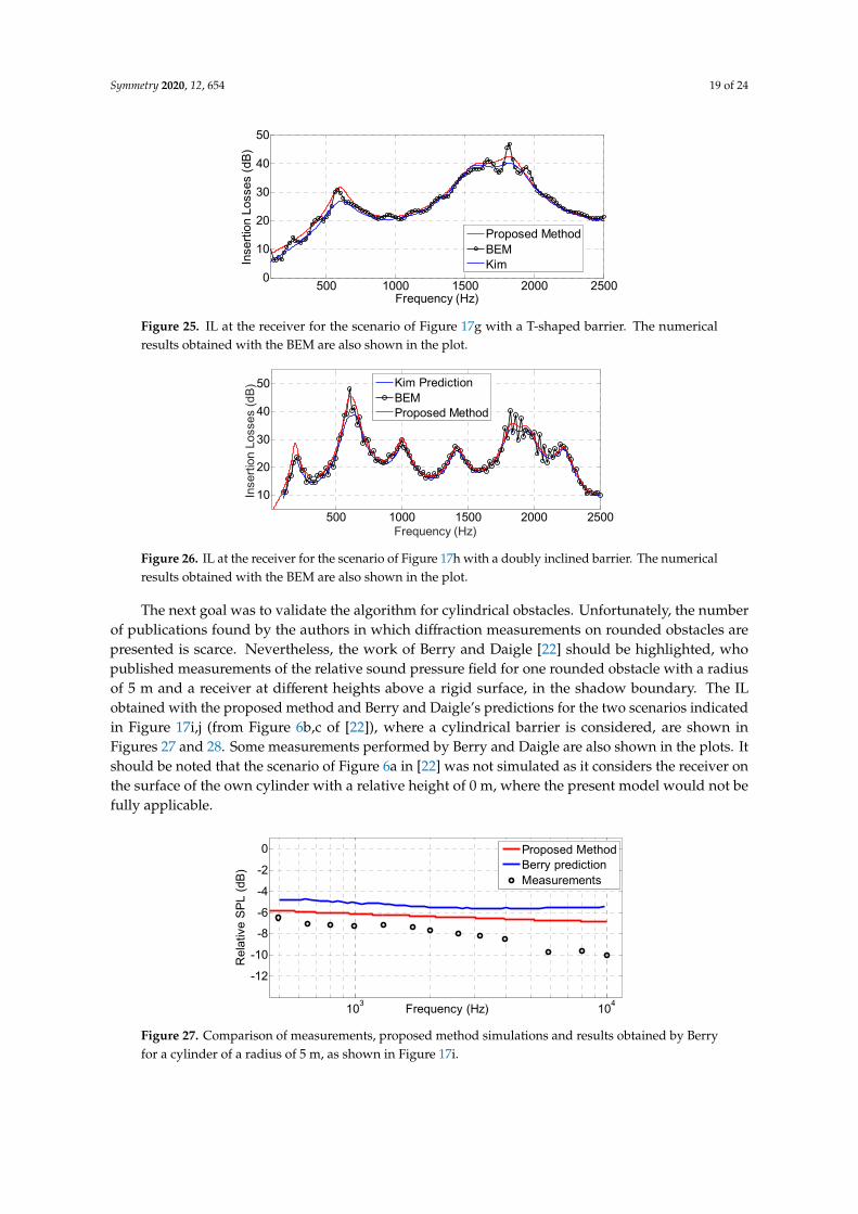
Symmetry 2020, 12, 654 19 of 24







500 1000 1500 2000 25000

20

40

60

Frequency (Hz)

Inse

rtion

Los

ses

(dB)


500 1000 1500 2000 25000

10

20

30

40

50

Frequency (Hz)

Inse

rtion

Los

ses

(dB)


500 1000 1500 2000 2500

10

20

30

40

50

Frequency (Hz)

Inse

rtion

Los

ses

(dB)


Figure 25. IL at the receiver for the scenario of Figure 17g with a T-shaped barrier. The numericalresults obtained with the BEM are also shown in the plot.







500 1000 1500 2000 25000

20

40

60

Frequency (Hz)

Inse

rtion

Los

ses

(dB)


500 1000 1500 2000 25000

10

20

30

40

50

Frequency (Hz)

Inse

rtion

Los

ses

(dB)


500 1000 1500 2000 2500

10

20

30

40

50

Frequency (Hz)

Inse

rtion

Los

ses

(dB)


Figure 26. IL at the receiver for the scenario of Figure 17h with a doubly inclined barrier. The numericalresults obtained with the BEM are also shown in the plot.

The next goal was to validate the algorithm for cylindrical obstacles. Unfortunately, the numberof publications found by the authors in which diffraction measurements on rounded obstacles arepresented is scarce. Nevertheless, the work of Berry and Daigle [22] should be highlighted, whopublished measurements of the relative sound pressure field for one rounded obstacle with a radiusof 5 m and a receiver at different heights above a rigid surface, in the shadow boundary. The ILobtained with the proposed method and Berry and Daigle’s predictions for the two scenarios indicatedin Figure 17i,j (from Figure 6b,c of [22]), where a cylindrical barrier is considered, are shown inFigures 27 and 28. Some measurements performed by Berry and Daigle are also shown in the plots. Itshould be noted that the scenario of Figure 6a in [22] was not simulated as it considers the receiver onthe surface of the own cylinder with a relative height of 0 m, where the present model would not befully applicable.


on the surface of the own cylinder with a relative height of 0 m, where the present model would not be fully applicable.

Figure 27. Comparison of measurements, proposed method simulations and results obtained by Berry for a cylinder of a radius of 5 m, as shown in Figure 17i.

Figure 28. Comparison of measurements, proposed method simulations and results obtained by Berry for a cylinder of a radius of 5 m, as shown in Figure 17j.

As can be observed, the proposed method shows better agreement with the measurements than the predictions of Berry and Daigle. The proposed method took 0.75 and 0.76 s to complete the plots of Figures 27 and 28, respectively (without considering reflections and 5000 frequency bins).

In order to also check the behavior of the algorithm for an array of rounded obstacles, a scenario filled with ten cylinders randomly allocated with different heights and the same radius was defined (Figure 29). Then, the IL results for cylindrical diffraction, without considering reflections on the ground, were compared with the asymptotic IL when the radius is decreased to almost 0 (knife edge case). It should be expected that the IL when considering cylinders would converge to the scenario where the obstacles are replaced by knife edges at the same locations and with the same heights. The results can be observed in Figure 30 for cylinders with radii of 1.0, 0.5 and 0.1 m.

103 104

-12

-10

-8

-6

-4

-2

0

Rel

ativ

e SP

L (d

B)

Frequency (Hz)

Proposed MethodBerry predictionMeasurements

103 104-15

-10

-5

0

Frequency (Hz)

Rel

ativ

e SP

L (d

B)


Figure 27. Comparison of measurements, proposed method simulations and results obtained by Berryfor a cylinder of a radius of 5 m, as shown in Figure 17i.

Symmetry 2020, 12, 654 20 of 24


on the surface of the own cylinder with a relative height of 0 m, where the present model would not be fully applicable.

Figure 27. Comparison of measurements, proposed method simulations and results obtained by Berry for a cylinder of a radius of 5 m, as shown in Figure 17i.

Figure 28. Comparison of measurements, proposed method simulations and results obtained by Berry for a cylinder of a radius of 5 m, as shown in Figure 17j.

As can be observed, the proposed method shows better agreement with the measurements than the predictions of Berry and Daigle. The proposed method took 0.75 and 0.76 s to complete the plots of Figures 27 and 28, respectively (without considering reflections and 5000 frequency bins).

In order to also check the behavior of the algorithm for an array of rounded obstacles, a scenario filled with ten cylinders randomly allocated with different heights and the same radius was defined (Figure 29). Then, the IL results for cylindrical diffraction, without considering reflections on the ground, were compared with the asymptotic IL when the radius is decreased to almost 0 (knife edge case). It should be expected that the IL when considering cylinders would converge to the scenario where the obstacles are replaced by knife edges at the same locations and with the same heights. The results can be observed in Figure 30 for cylinders with radii of 1.0, 0.5 and 0.1 m.

103 104

-12

-10

-8

-6

-4

-2

0

Rel

ativ

e SP

L (d

B)

Frequency (Hz)


103 104-15

-10

-5

0

Frequency (Hz)

Rel

ativ

e SP

L (d

B)


Figure 28. Comparison of measurements, proposed method simulations and results obtained by Berryfor a cylinder of a radius of 5 m, as shown in Figure 17j.

As can be observed, the proposed method shows better agreement with the measurements thanthe predictions of Berry and Daigle. The proposed method took 0.75 and 0.76 s to complete the plots ofFigures 27 and 28, respectively (without considering reflections and 5000 frequency bins).

In order to also check the behavior of the algorithm for an array of rounded obstacles, a scenariofilled with ten cylinders randomly allocated with different heights and the same radius was defined(Figure 29). Then, the IL results for cylindrical diffraction, without considering reflections on theground, were compared with the asymptotic IL when the radius is decreased to almost 0 (knife edgecase). It should be expected that the IL when considering cylinders would converge to the scenariowhere the obstacles are replaced by knife edges at the same locations and with the same heights.The results can be observed in Figure 30 for cylinders with radii of 1.0, 0.5 and 0.1 m.Symmetry 2020, 12, x FOR PEER REVIEW 21 of 25

Figure 29. Scenario with ten cylinders randomly located between the tx and rx. The Fresnel ellipsoids at 100 Hz are superimposed in the profile.

Figure 30. Comparison of the scenario depicted on top assuming knife edges and cylinders with decreasing radii. Reflections on the ground are not considered in this case.

As expected, the curves for the knife edges case and cylinders with a radius of 0.1 m practically coincide.

Analysis of Computational Efficiency of the Proposed Method

In order to analyze the computational efficiency of the proposed method, we will consider again the scenario of Figure 17e with three barriers, whose IL results are already shown in Figure 23. The full elapsed time to plot the whole IL results with our method (assuming 2500 frequency bins) was only 13.89 s, taking advantage of the funicular profiles, an optimum choice of nodes as a function of frequency by Fresnel ellipsoids, graph theory for the fast search and reordering of paths by number of hops and a threshold value to account for any path. In contrast, the time employed for the Min and Qiu method, for only one frequency and the same computer, was 2.6 min, which points to a much greater simulation time. The BEM results, which are frequency-dependent, such as OpenBEM [23], required more than half an hour per a single frequency bin and the same scenario of Figure 17e, which again is a much longer time compared to the method proposed in this work.

Moreover, in order to check the impact on accuracy of the IL estimated with our method when the maximum number of hops in the path is progressively reduced, Figure 31 is shown, where again the scenario of Figure 17e is considered. On this basis, the maximum number of hops in the scenario is progressively constrained (down to only seven hops) and a threshold criterion to add new paths is also kept (10−5). It should be noted that three wide barriers imply a maximum number of 12 nodes and 11 hops, including reflections.

0 2 4 6 8 10 12 14 16 18 200

2

4

6

8

10

Hei

ght (

m)

Distance (m)

500 1000 1500 2000 2500 3000 3500 4000 4500 500030

40

50

60

70

80

90

Frequency (Hz)

Inse

rtion

Los

ses

(dB)

Knife-edgesRadii=1.0 mRadii=0.5 mRadii=0.1 m

Figure 29. Scenario with ten cylinders randomly located between the tx and rx. The Fresnel ellipsoidsat 100 Hz are superimposed in the profile.


Figure 29. Scenario with ten cylinders randomly located between the tx and rx. The Fresnel ellipsoids at 100 Hz are superimposed in the profile.

Figure 30. Comparison of the scenario depicted on top assuming knife edges and cylinders with decreasing radii. Reflections on the ground are not considered in this case.

As expected, the curves for the knife edges case and cylinders with a radius of 0.1 m practically coincide.


In order to analyze the computational efficiency of the proposed method, we will consider again the scenario of Figure 17e with three barriers, whose IL results are already shown in Figure 23. The full elapsed time to plot the whole IL results with our method (assuming 2500 frequency bins) was only 13.89 s, taking advantage of the funicular profiles, an optimum choice of nodes as a function of frequency by Fresnel ellipsoids, graph theory for the fast search and reordering of paths by number of hops and a threshold value to account for any path. In contrast, the time employed for the Min and Qiu method, for only one frequency and the same computer, was 2.6 min, which points to a much greater simulation time. The BEM results, which are frequency-dependent, such as OpenBEM [23], required more than half an hour per a single frequency bin and the same scenario of Figure 17e, which again is a much longer time compared to the method proposed in this work.

Moreover, in order to check the impact on accuracy of the IL estimated with our method when the maximum number of hops in the path is progressively reduced, Figure 31 is shown, where again the scenario of Figure 17e is considered. On this basis, the maximum number of hops in the scenario is progressively constrained (down to only seven hops) and a threshold criterion to add new paths is also kept (10−5). It should be noted that three wide barriers imply a maximum number of 12 nodes and 11 hops, including reflections.

0 2 4 6 8 10 12 14 16 18 200

2

4

6

8

10

Hei

ght (

m)

Distance (m)

500 1000 1500 2000 2500 3000 3500 4000 4500 500030

40

50

60

70

80

90

Frequency (Hz)

Inse

rtion

Los

ses

(dB)

Knife-edgesRadii=1.0 mRadii=0.5 mRadii=0.1 m

Figure 30. Comparison of the scenario depicted on top assuming knife edges and cylinders withdecreasing radii. Reflections on the ground are not considered in this case.

As expected, the curves for the knife edges case and cylinders with a radius of 0.1 mpractically coincide.

Symmetry 2020, 12, 654 21 of 24


In order to analyze the computational efficiency of the proposed method, we will consider againthe scenario of Figure 17e with three barriers, whose IL results are already shown in Figure 23. The fullelapsed time to plot the whole IL results with our method (assuming 2500 frequency bins) was only13.89 s, taking advantage of the funicular profiles, an optimum choice of nodes as a function offrequency by Fresnel ellipsoids, graph theory for the fast search and reordering of paths by number ofhops and a threshold value to account for any path. In contrast, the time employed for the Min andQiu method, for only one frequency and the same computer, was 2.6 min, which points to a muchgreater simulation time. The BEM results, which are frequency-dependent, such as OpenBEM [23],required more than half an hour per a single frequency bin and the same scenario of Figure 17e, whichagain is a much longer time compared to the method proposed in this work.

Moreover, in order to check the impact on accuracy of the IL estimated with our method when themaximum number of hops in the path is progressively reduced, Figure 31 is shown, where again thescenario of Figure 17e is considered. On this basis, the maximum number of hops in the scenario isprogressively constrained (down to only seven hops) and a threshold criterion to add new paths is alsokept (10−5). It should be noted that three wide barriers imply a maximum number of 12 nodes and11 hops, including reflections.Symmetry 2020, 12, x FOR PEER REVIEW 22 of 25

Figure 31. Comparison of IL for scenario of Figure 17e with Min and Qiu’s prediction, BEM and the proposed method when decreasing the number of possible hops in the path.

As can be observed, even when the maximum number of hops is decreased down to seven or eight hops, the accuracy of the results obtained with the proposed method remains reasonable whilst simultaneously reducing the computational effort down to only 10 s (when limiting the maximum number of hops to eight).

Finally, in order to assess the potential and the efficiency in terms of computational time of the proposed method to estimate the IL at the receiver as a function of frequency, a completely heterogeneous and more complex scenario is finally considered in Figure 32, in which different types of obstacle modeling, heights and spacing are taken into account. When running the method, one obstacle is initially discarded at 200 Hz by the application of the Fresnel criterion at the distance of 15.2 m and 20 nodes. The transmitter, obstacles, reflections and receiver are then considered.

Figure 32. Complex scenario with nine different barriers. One is discarded by Fresnel criterion at the distance of 15.2 m.

The IL as a function of frequency, with and without reflections on the ground, is shown in Figure 33.

Figure 33. IL spectrum for scenario of Figure 32 with and without reflections.

The parameters of the simulations of Figure 33 and the obtained results are summarized in Table 1.

Table 1. Parameters for Scenario of Figure 32.

0 1000 2000 3000 4000-20

0

20

40

60

Frequency (Hz)

Inse

rtion

Los

ses

(dB)

BEM data7 hops8 hops9 hops10 hopsAll hopsMin prediction

0 1000 2000 3000 4000 500040

60

80

100

Frequency (Hz)

Inse

rtion

Los

ses

(dB)

Without reflectionWith reflection

Figure 31. Comparison of IL for scenario of Figure 17e with Min and Qiu’s prediction, BEM and theproposed method when decreasing the number of possible hops in the path.

As can be observed, even when the maximum number of hops is decreased down to seven oreight hops, the accuracy of the results obtained with the proposed method remains reasonable whilstsimultaneously reducing the computational effort down to only 10 s (when limiting the maximumnumber of hops to eight).

Finally, in order to assess the potential and the efficiency in terms of computational time ofthe proposed method to estimate the IL at the receiver as a function of frequency, a completelyheterogeneous and more complex scenario is finally considered in Figure 32, in which different typesof obstacle modeling, heights and spacing are taken into account. When running the method, oneobstacle is initially discarded at 200 Hz by the application of the Fresnel criterion at the distance of 15.2m and 20 nodes. The transmitter, obstacles, reflections and receiver are then considered.










0 1000 2000 3000 4000-20

0

20

40

60

Frequency (Hz)

Inse

rtion

Los

ses

(dB)


0 1000 2000 3000 4000 500040

60

80

100

Frequency (Hz)

Inse

rtion

Los

ses

(dB)


Figure 32. Complex scenario with nine different barriers. One is discarded by Fresnel criterion at thedistance of 15.2 m.

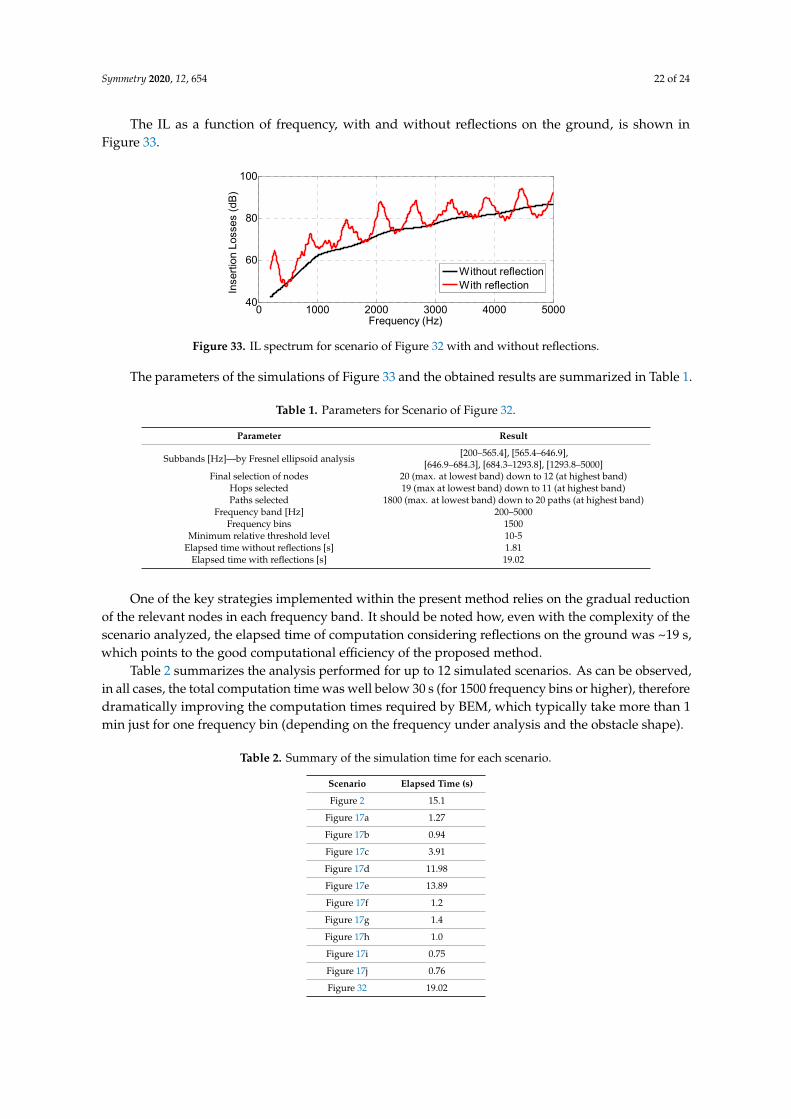
Symmetry 2020, 12, 654 22 of 24

The IL as a function of frequency, with and without reflections on the ground, is shown inFigure 33.










0 1000 2000 3000 4000-20

0

20

40

60

Frequency (Hz)

Inse

rtion

Los

ses

(dB)


0 1000 2000 3000 4000 500040

60

80

100

Frequency (Hz)

Inse

rtion

Los

ses

(dB)





Parameter Result

Subbands [Hz]—by Fresnel ellipsoid analysis [200–565.4], [565.4–646.9],[646.9–684.3], [684.3–1293.8], [1293.8–5000]

Final selection of nodes 20 (max. at lowest band) down to 12 (at highest band)Hops selected 19 (max at lowest band) down to 11 (at highest band)Paths selected 1800 (max. at lowest band) down to 20 paths (at highest band)

Frequency band [Hz] 200–5000Frequency bins 1500

Minimum relative threshold level 10-5Elapsed time without reflections [s] 1.81

Elapsed time with reflections [s] 19.02

One of the key strategies implemented within the present method relies on the gradual reductionof the relevant nodes in each frequency band. It should be noted how, even with the complexity of thescenario analyzed, the elapsed time of computation considering reflections on the ground was ~19 s,which points to the good computational efficiency of the proposed method.

Table 2 summarizes the analysis performed for up to 12 simulated scenarios. As can be observed,in all cases, the total computation time was well below 30 s (for 1500 frequency bins or higher), thereforedramatically improving the computation times required by BEM, which typically take more than 1min just for one frequency bin (depending on the frequency under analysis and the obstacle shape).

Table 2. Summary of the simulation time for each scenario.

Scenario Elapsed Time (s)

Figure 2 15.1

Figure 17a 1.27

Figure 17b 0.94

Figure 17c 3.91

Figure 17d 11.98

Figure 17e 13.89

Figure 17f 1.2

Figure 17g 1.4

Figure 17h 1.0

Figure 17i 0.75

Figure 17j 0.76

Figure 32 19.02

Symmetry 2020, 12, 654 23 of 24

4. Conclusions

In this work, an innovative, fast, UTD-based method for the analysis of multiple diffraction ofacoustic waves when considering a series of obstacles with arbitrary modeling (knife edges, wedges,wide barriers, cylinders, doubly inclined and T-/Y-shaped barriers), height and spacing has beenpresented. The method, which makes use of funicular polygons, Fresnel ellipsoids and graph theory,and controls both the maximum number of hops and the minimum threshold criterium, has beenproperly compared and validated with other existing formulations as well as measurements showinggood agreement while at the same time offering much better computational efficiency. On this basis,a great number of obstacles (including neighboring ones of equal height) forming a very complexscenario can be analyzed in an acceptable time.

The potential of the proposed method in terms of computational time is due to the fact that itallows for an optimum selection of the prominent obstacles, processes them as nodes of a graph,identifies and rearranges the paths reaching the receiver, constraints the maximum number of hopsand permits defining a threshold criterion to discern the relevant paths.

Future work will be focused on the performance of an extensive measurement campaignundertaken in real scenarios to explore the limits in which the proposed method remains valid.Moreover, the authors’ future interest will be paid on reviewing, extending and validating the presentmethod for more complex scenarios involving 3D profiles, as well as other polygonal structures whilefurther achieving improved computational efficiency. Finally, the authors’ attention will also includethe characterization of the acoustic impedance of the barriers for extending the model to a wider rangeof scenarios and applications.

Author Contributions: Conceptualization, D.P.-Q. and J.-V.R.; methodology, D.P.-Q.; software, D.P.-Q.; validation,D.P.-Q.; formal analysis, D.P.-Q.; investigation, D.P.-Q. and J.-V.R.; resources, D.P.-Q. and J.-V.R.; data curation,D.P.-Q.; writing—original draft preparation, D.P.-Q.; writing—review and editing, D.P.-Q. and J.-V.R.; visualization,D.P.-Q. and J.-V.R.; supervision, J.-V.R.; project administration, J.-V.R.; funding acquisition, J.-V.R. All authors haveread and agreed to the published version of the manuscript.

Funding: This work has been funded by the Ministerio de Economía y Competitividad (MINECO), Spain(TEC2016-78028-C3-2-P), and by European Fonds Européen de Développement Économique et Régional(FEDER) funds.

Conflicts of Interest: The authors declare no conflict of interest. The funders had no role in the design of thestudy, in the collection, analyses, or interpretation of data, in the writing of the manuscript or in the decision topublish the results.

References

1. Seznec, R. Diffraction of sound around barriers: Use of the boundary elements technique. J. Sound Vib. 1980,73, 195–209. [CrossRef]

2. Salomons, E.M. Diffraction by a screen in downwind sound propagation: A parabolic equation approach.J. Acoust. Soc. Am. 1994, 95, 3109. [CrossRef]

3. Pierce, A.D. Diffraction of sound around corners and over wide barriers. J. Acoust. Soc. Am. 1974, 55, 941–955.[CrossRef]

4. Kawai, T. Sound diffraction by a many-sided barrier or pillar. J. Sound Vib. 1981, 79, 229–242. [CrossRef]5. Kim, H.S.; Kim, J.S.; Kang, H.J.; Kim, B.K.; Kim, S.R. Sound diffraction by multiple wedges and thin screens.

Appl. Acoust. 2005, 66, 1102–1119. [CrossRef]6. Min, H.; Qiu, X. Multiple acoustic diffraction around rigid parallel wide barriers. J. Acoust. Soc. Am. 2009,

126, 179–186. [CrossRef]7. Rodríguez, J.-V.; Pascual-García, J.; Martínez-Inglés, M.-T.; Molina-Garcia-Pardo, J.-M.; Juan-Llácer, L.

Uniform theory of diffraction (UTD)-based solution for sound diffraction caused by an array of obstacles.J. Acoust. Soc. Am. 2017, 142, 902–907. [CrossRef]

8. Pardo-Quiles, D.; Rodríguez, J.-V.; Lozano-Giménez, R.; Juan-Llácer, L.; Pascual-García, J. On the influence ofobstacle modeling in multiple diffraction of acoustic waves. Acta Acust. Acust. 2019, 105, 261–264. [CrossRef]

9. Kurze, U.J.; Anderson, G.S. Sound attenuation by barriers. Appl. Acoust. 1971, 4, 35–53. [CrossRef]

http://dx.doi.org/10.1016/0022-460X(80)90689-6

http://dx.doi.org/10.1121/1.410002

http://dx.doi.org/10.1121/1.1914668

http://dx.doi.org/10.1016/0022-460X(81)90370-9

http://dx.doi.org/10.1016/j.apacoust.2005.01.004

http://dx.doi.org/10.1121/1.3147491

http://dx.doi.org/10.1121/1.4997942

http://dx.doi.org/10.3813/AAA.919308

http://dx.doi.org/10.1016/0003-682X(71)90024-7

Symmetry 2020, 12, 654 24 of 24

10. Keller, B. Geometrical theory of diffraction. J. Opt. Soc. Am. 1962, 52, 116–130. [CrossRef] [PubMed]11. Kouyoumjian, R.G.; Pathak, P.H. A uniform geometrical theory of diffraction for an edge in a perfectly

conducting surface. Proc. IEEE 1974, 62, 1448–1461. [CrossRef]12. Hadden, W.J.; Pierce, A.D. Sound diffraction around screens and wedges for arbitrary point source location.

J. Acoust. Soc. Am. 1981, 69, 1266–1276. [CrossRef]13. Kapralos, B.; Milos, E.; Jenkin, M. Acoustical diffraction modeling utilizing the Huygens-Fresnel principle.

In Proceedings of the IEEE International Workshop on Haptic Audio Visual Environments and theirApplications, Ottawa, ON, Canada, 1 October 2005; Volume 6. [CrossRef]

14. Bollobas, B. Modern Graph Theory; Springer: Berlin, Germany, 1998.15. West, D. Introduction to Graph Theory, 2nd ed.; Prentice Hall: Upper Saddle River, NJ, USA, 2000.16. Jungnickel, D. Graphs, Networks and Algorithms, Algorithms and Computation in Mathematics; Springer: Berlin,

Germany, 2005; Volume 5.17. McNamara, D.A.; Pistorius, C.W.I.; Malherbe, J.A.G. Introduction to the Uniform Geometrical Theory of Diffraction;

Artech House: Norwood, MA, USA, 1990.18. Koutitas, G.; Tzaras, C. A UTD solution for multiple rounded surfaces. IEEE Trans. Antennas Propag. 2006,

54, 4. [CrossRef]19. Rodríguez, J.-V.; Molina-Garcia-Pardo, J.-M.; Juan-Llácer, L. A hybrid UTD-PO solution for multiple-cylinder

diffraction analysis assuming spherical-wave incidence. IEEE Trans. Antennas Propag. 2008, 56, 3078–3081.[CrossRef]

20. MATLAB. Version 8.5.0 (R2015a); The MathWorks Inc.: Natick, MA, USA, 2015.21. Wadsworth, G.J.; Chambers, J.P. Scale model experiments on the insertion loss of wide and double barriers.

J. Acoust. Soc. Am. 2000, 107, 2344–2350. [CrossRef] [PubMed]22. Berry, A.; Daigle, G.A. Controlled experiments of the diffraction of sound by a curved surface. J. Acoust. Soc.

Am. 1998, 83, 2047–2058. [CrossRef] [PubMed]23. Henríquez, V.C.; Juhl, P.M. OpenBEM—An Open Source Boundary Element Method Software in Acoustics.

In Proceedings of the 39th Internoise, Lisbon, Portugal, 13 June 2010.

© 2020 by the authors. Licensee MDPI, Basel, Switzerland. This article is an open accessarticle distributed under the terms and conditions of the Creative Commons Attribution(CC BY) license (http://creativecommons.org/licenses/by/4.0/).

http://dx.doi.org/10.1364/JOSA.52.000116

http://www.ncbi.nlm.nih.gov/pubmed/14454948

http://dx.doi.org/10.1109/PROC.1974.9651

http://dx.doi.org/10.1121/1.385809

http://dx.doi.org/10.1109/HAVE.2005.1545649

http://dx.doi.org/10.1109/TAP.2006.872675

http://dx.doi.org/10.1109/TAP.2008.928817

http://dx.doi.org/10.1121/1.428620


http://dx.doi.org/10.1121/1.396385


http://creativecommons.org/

http://creativecommons.org/licenses/by/4.0/.

A Fast UTD-Based Method for the Analysis of Multiple ... - MDPI

Documents

Transcript of A Fast UTD-Based Method for the Analysis of Multiple ... - MDPI