Citation: Hu, Z.; Wu, Q.; Zou, J.;

Wan, Q. Fast and Efficient

Two-Dimensional DOA Estimation

for Signals with Known Waveforms

Using Uniform Circular Array. Appl.

Sci. 2022, 12, 4007. https://doi.org/

10.3390/app12084007

Academic Editor: Amalia Miliou

Received: 16 March 2022

Accepted: 13 April 2022

Published: 15 April 2022

Publisher’s Note: MDPI stays neutral

with regard to jurisdictional claims in

published maps and institutional affil-

iations.

Copyright: © 2022 by the authors.

Licensee MDPI, Basel, Switzerland.

This article is an open access article

distributed under the terms and

conditions of the Creative Commons

Attribution (CC BY) license (https://

creativecommons.org/licenses/by/

4.0/).

applied sciences

Article

Fast and Efficient Two-Dimensional DOA Estimation forSignals with Known Waveforms Using Uniform Circular ArrayZepeng Hu , Qi Wu, Jifeng Zou and Qun Wan *

School of Information and Communication Engineering, University of Electronic Science and Technology of China,Chengdu 611731, China; huzepeng@std.uestc.edu.cn (Z.H.); wuqi57@std.uestc.edu.cn (Q.W.);jifengzou@163.com (J.Z.)* Correspondence: wanqun@uestc.edu.cn

Abstract: This paper addresses the two-dimensional (2D) direction-of-arrival (DOA) estimation issuefor signals with known waveforms but unknown amplitudes using uniform circular array (UCA).Unlike maximum likelihood (ML) methods such as decoupled maximum likelihood (DEML), paralleldecomposition (PADEC) and so forth, which estimate DOA by spectrum peak search, we propose anefficient interferometer-based method with known waveforms. The proposed method first estimatesspatial signature matrix based on ML method whose each column contains 2D DOA informationcorresponding to a source. Then, an interferometer procedure is performed to obtain 2D DOAestimate of each source from a closed-form solution separately and in parallel. Several simulationresults show that the proposed method can achieve a significantly improvement in performancethat coincides with the ML method as well as Cramér-Rao Bound (CRB), especially under somepoor conditions, such as low SNR, fewer sensors or small snapshots. In addition, the performancewill not degrade as the number of sources increases if the source signals are uncorrelated with eachother. Meanwhile, it reduces a great amount of computational complexity without loss of too muchaccuracy. Thus, the proposed method is quite suitable for 2D DOA estimation with known waveformsin practice.

Keywords: two-dimensional direction of arrival; known waveform; uniform circular array; interfer-ometer; Cramér-Rao Bound

1. Introduction

Direction of arrival (DOA) estimation has been applied to a variety of civil and militaryfields, such as communications, sonar, air traffic control, electronic reconnaissance, etc. inthe past decades [1,2]. A great many DOA estimation algorithms have been proposed,including beamforming-based methods [3], subspace-based methods [4–6] and sparsity-based methods [7–9]. These techniques generally consider the source signals to be non-cooperative signals and mainly utilize spatial properties such as the auto-correlation matrix,without taking into account any prior information. However, abundant prior informationon signals of interest may be available to achieve better performance in mobile wirelesscommunications, active radar or sonar, and many other applications; for example, knownsignal waveforms can be exploited to significantly improve DOA estimation accuracy,eliminate interfering signals and simplify computational complexity [10].

A series of algorithms have been developed in recent decades to deal with the problemof DOA estimation with known waveforms, including decoupled maximum likelihood(DEML) [11], coherent decoupled maximum likelihood (CDEML) [12], white coherentdecoupled maximum likelihood (WCDEML) [13], parallel decomposition (PADEC) [14],subarray beamforming-based DOA (SBDOA) [15], linear operators (LP) [16] and morerecent research [17–23]. The previous papers have proven that the Cramér-Rao Bound(CRB) and root-mean-square error (RMSE) of DOA estimation for signals with knownwaveforms are much lower than those with unknown waveforms [10,11].

Appl. Sci. 2022, 12, 4007. https://doi.org/10.3390/app12084007 https://www.mdpi.com/journal/applsci

Appl. Sci. 2022, 12, 4007 2 of 15

Note that these algorithms mainly focus on using a uniform linear array (ULA) [15],sparse linear array (SLA) [18] or nonuniform linear array [19] to estimate signals’ one-dimensional (1D) DOA. However, a linear array only provides 180 azimuthal coverage,while a planar array is a more attractive configuration known for its ability to provide360 azimuthal coverage and elevation angle information in addition. Moreover, when itcomes to using a planar array such as uniform circular array (UCA) to estimate the abovetwo-dimensional (2D) DOA, some algorithms specially designed for ULA, such as [6,14–16],may become invalid or need some complicated transformations [24].

On the other hand, the existing DOA estimators with known waveforms are ofteninvolved in eigenvalue decomposition [14], finding polynomial roots [13] or spectrumpeak search [22], the computational complexity of which is too burdensome to realizein practice. In fact, interferometer-based methods are more suitable and widely usedfor DOA estimation with advantages of higher efficiency, broader flexibility and easierrealization [25–29]. Up to now, there has been only one study concerning an interferometer-based DOA estimator with a known waveform [30]; however, it was only designed for onesource using ULA.

In view of the above two aspects, we take advantage of the interferometer method tosolve the 2D DOA estimation problem considering multiple sources with known waveformsusing UCA. Extension to other planar arrays, such as uniform rectangular array, L-shapearray, etc., is similar and straightforward. The main idea of our method is to exploit auto-correlation and cross-correlation matrix of known waveforms and array output vectorsto estimate spatial signature matrix at first. Due to the fact that each column of spatialsignature matrix is colinear with steering vector of one source, each 2D DOA is estimatedthrough an interferometer procedure separately and in parallel. The proposed method iscomputationally efficient and easy to implement in practice, as all 2D DOA estimates areobtained in closed form from a series of least-squared (LS) solutions without searching theparameter space. Furthermore, we also derive the corresponding CRB of 2D DOA withknown waveforms to prove the effectiveness of our method. Simulation results show thatthe performance of the proposed method achieves the ML method as well as the CRB undermost circumstances, with the benefit of much less computational demand.

The rest of the paper is arranged as follows. Section 2 gives the model of the arrayoutput signals of UCA and known waveforms, along with some necessary assumptions.Section 3 introduces the ML and interferometer-based DOA estimator with known wave-forms, respectively. Section 4 recalls CRB of 2D DOA without known waveforms andderives CRB with known waveforms. Section 5 carries out several simulations to verify theproposed method. Conclusions are summarized in Section 6.

The following notations are used in the paper: matrices and vectors are denotedby bold upper-case and lower-case letters, respectively. (·)T , (·)∗, (·)H and (·)−1 denotetranspose, conjugate, conjugate transpose and inverse, respectively. E·, diag·, || · || and denote expectation, diagonalization, Euclidean norm and Hadamard product. | · |, Re·(or

_(·)), Im· (or

^(·)) and arg· denote modulus, real part, imaginary part and argument

of a complex number, respectively. I and 0 denote identity and zero matrix of proper size.

2. Signal Model

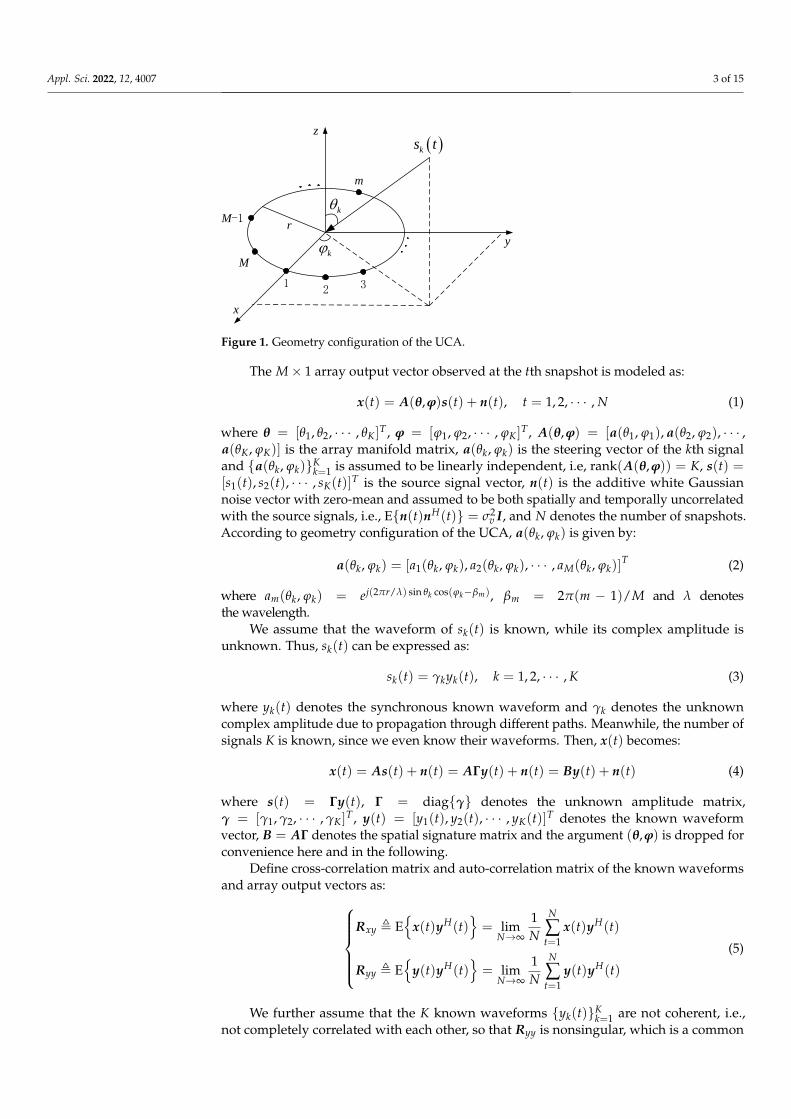
Consider a UCA with radius r and M(M > K) isotropic sensors uniformly distributedover the circumference in the xy-plane, the geometry configuration of which is depictedin Figure 1. Assume that there are K co-frequency far-field narrowband signals imping-ing on the UCA from distinct angles (θ1, ϕ1), (θ2, ϕ2), · · · , (θK, ϕK), where θk ∈ [0, π/2)and ϕk ∈ [−π, π) are elevation and azimuth angle of the k-th signal, respectively. Theelevation angle is measured downward from the z-axis and the azimuth angle is measuredcounterclockwise from the x-axis.

Appl. Sci. 2022, 12, 4007 3 of 15

x

y

z

21 3

k

k

( )ks t

M-1

M

m

r

Figure 1. Geometry configuration of the UCA.

The M× 1 array output vector observed at the tth snapshot is modeled as:

x(t) = A(θ,ϕ)s(t) + n(t), t = 1, 2, · · · , N (1)

where θ = [θ1, θ2, · · · , θK]T , ϕ = [ϕ1, ϕ2, · · · , ϕK]

T , A(θ,ϕ) = [a(θ1, ϕ1), a(θ2, ϕ2), · · · ,a(θK, ϕK)] is the array manifold matrix, a(θk, ϕk) is the steering vector of the kth signaland a(θk, ϕk)K

k=1 is assumed to be linearly independent, i.e, rank(A(θ,ϕ)) = K, s(t) =[s1(t), s2(t), · · · , sK(t)]T is the source signal vector, n(t) is the additive white Gaussiannoise vector with zero-mean and assumed to be both spatially and temporally uncorrelatedwith the source signals, i.e., En(t)nH(t) = σ2

v I, and N denotes the number of snapshots.According to geometry configuration of the UCA, a(θk, ϕk) is given by:

a(θk, ϕk) = [a1(θk, ϕk), a2(θk, ϕk), · · · , aM(θk, ϕk)]T (2)

where am(θk, ϕk) = ej(2πr/λ) sin θk cos(ϕk−βm), βm = 2π(m − 1)/M and λ denotesthe wavelength.

We assume that the waveform of sk(t) is known, while its complex amplitude isunknown. Thus, sk(t) can be expressed as:

sk(t) = γkyk(t), k = 1, 2, · · · , K (3)

where yk(t) denotes the synchronous known waveform and γk denotes the unknowncomplex amplitude due to propagation through different paths. Meanwhile, the number ofsignals K is known, since we even know their waveforms. Then, x(t) becomes:

x(t) = As(t) + n(t) = AΓy(t) + n(t) = By(t) + n(t) (4)

where s(t) = Γy(t), Γ = diagγ denotes the unknown amplitude matrix,γ = [γ1, γ2, · · · , γK]

T , y(t) = [y1(t), y2(t), · · · , yK(t)]T denotes the known waveformvector, B = AΓ denotes the spatial signature matrix and the argument (θ,ϕ) is dropped forconvenience here and in the following.

Define cross-correlation matrix and auto-correlation matrix of the known waveformsand array output vectors as:

Rxy , E

x(t)yH(t)= lim

N→∞

1N

N

∑t=1

x(t)yH(t)

Ryy , E

y(t)yH(t)= lim

N→∞

1N

N

∑t=1

y(t)yH(t)

(5)

We further assume that the K known waveforms yk(t)Kk=1 are not coherent, i.e.,

not completely correlated with each other, so that Ryy is nonsingular, which is a common

Appl. Sci. 2022, 12, 4007 4 of 15

situation in communications. In addition, the source signals and noise are assumed to beuncorrelated, i.e., Rny = 0, where Rny is defined similarly.

The problem of interest herein is to estimate the elevation angle θ and the azimuthangle ϕ from the array output vectors x(t)N

t=1 and the known waveforms y(t)Nt=1.

3. Direction-of-Arrival Estimators with Known Waveforms

In this section, we first derive the maximum likelihood (ML) DOA estimator forsignals with known waveforms, then the interferometer-based DOA estimator with knownwaveforms is proposed intuitively.

3.1. Maximum Likelihood Estimator with Known Waveforms

We regard the source signals as deterministic process due to known waveforms, hence,likelihood function of x(t)N

t=1 is:

P(θ,ϕ, γ, σ2v ) =

N

∏t=1

1(πσ2

v )M exp

− 1

σ2v||x(t)− By(t)||2

=

1(πσ2

v )MN exp

− 1

σ2v

N

∑t=1||x(t)− By(t)||2

(6)

Since the noise in (1) is a zero-mean white Gaussian random process, it is obvious thatmaximizing the likelihood function with respect to θ, ϕ and γ is equivalent to minimizingthe following cost function:

L(θ,ϕ, γ) =N

∑t=1||x(t)− By(t)||2 (7)

In this case, the LS approach is the same as the ML method [31], so that the LS or MLestimate of B is given as follows:

B =

(N

∑t=1

x(t)yH(t)

)(N

∑t=1

y(t)yH(t)

)−1

= RxyR−1yy

(8)

where Rxy = 1/N ∑Nt=1 x(t)yH(t) and Ryy = 1/N ∑N

t=1 y(t)yH(t) are estimates of auto-correlation and cross-correlation. As Ryy is nonsingular, so does Ryy when N is largeenough. It is easy to find that B is a asymptotic consistent estimate of B:

limN→∞

B = limN→∞

RxyR−1yy

= limN→∞

[1N

N

∑t=1

(By(t) + n(t))yH(t)

]R−1

yy

= limN→∞

(BRyy + Rny

)R−1

yy

= B

(9)

where limN→∞

Rny = Rny = 0 since the noise vectors and the known waveforms

are uncorrelated.Once we obtain B, based on above analysis and the structure of B, i.e., bk = γka(θk, ϕk),

where bk is the kth column of B, the problem of ML estimation of θ and ϕ is decoupled intoK independent maximization problems as follows:(

θk, ϕk)= arg max

θ,ϕ|aH(θ, ϕ)bk|2, k = 1, 2, · · · , K (10)

Appl. Sci. 2022, 12, 4007 5 of 15

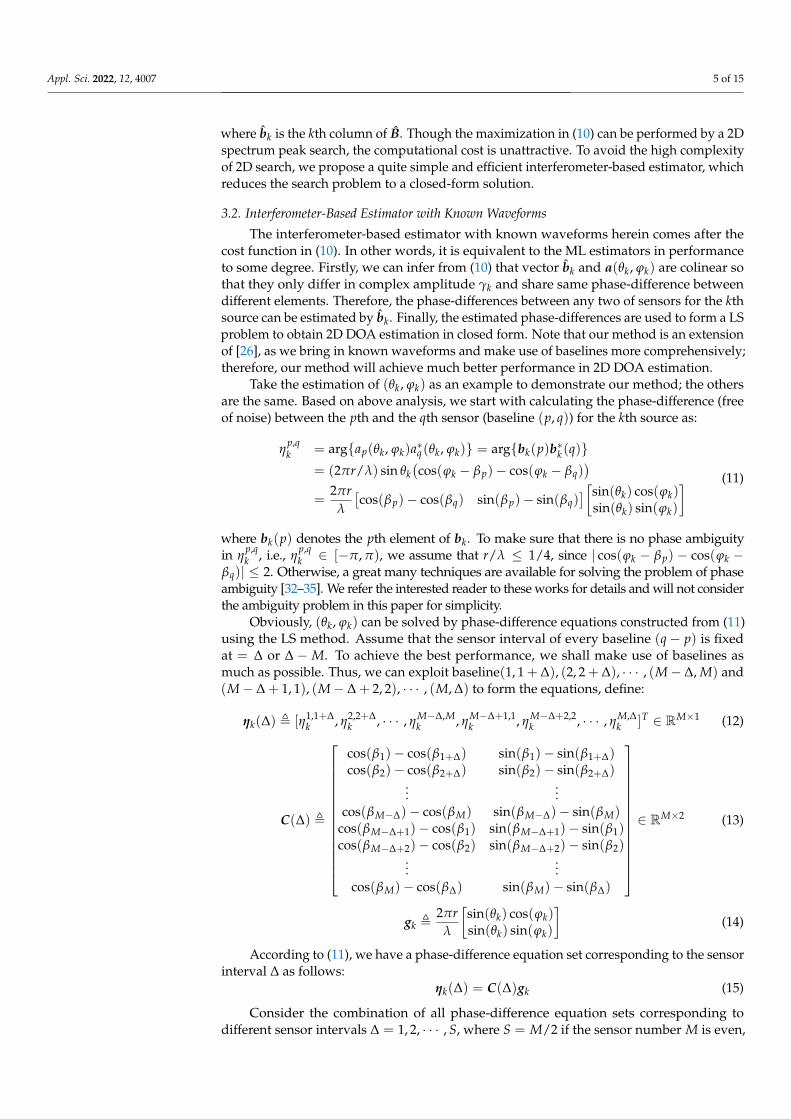
where bk is the kth column of B. Though the maximization in (10) can be performed by a 2Dspectrum peak search, the computational cost is unattractive. To avoid the high complexityof 2D search, we propose a quite simple and efficient interferometer-based estimator, whichreduces the search problem to a closed-form solution.

3.2. Interferometer-Based Estimator with Known Waveforms

The interferometer-based estimator with known waveforms herein comes after thecost function in (10). In other words, it is equivalent to the ML estimators in performanceto some degree. Firstly, we can infer from (10) that vector bk and a(θk, ϕk) are colinear sothat they only differ in complex amplitude γk and share same phase-difference betweendifferent elements. Therefore, the phase-differences between any two of sensors for the kthsource can be estimated by bk. Finally, the estimated phase-differences are used to form a LSproblem to obtain 2D DOA estimation in closed form. Note that our method is an extensionof [26], as we bring in known waveforms and make use of baselines more comprehensively;therefore, our method will achieve much better performance in 2D DOA estimation.

Take the estimation of (θk, ϕk) as an example to demonstrate our method; the othersare the same. Based on above analysis, we start with calculating the phase-difference (freeof noise) between the pth and the qth sensor (baseline (p, q)) for the kth source as:

ηp,qk = argap(θk, ϕk)a∗q(θk, ϕk) = argbk(p)b∗k (q)

= (2πr/λ) sin θk(cos(ϕk − βp)− cos(ϕk − βq)

)=

2πrλ

[cos(βp)− cos(βq) sin(βp)− sin(βq)

][sin(θk) cos(ϕk)sin(θk) sin(ϕk)

] (11)

where bk(p) denotes the pth element of bk. To make sure that there is no phase ambiguityin η

p,qk , i.e., η

p,qk ∈ [−π, π), we assume that r/λ ≤ 1/4, since | cos(ϕk − βp) − cos(ϕk −

βq)| ≤ 2. Otherwise, a great many techniques are available for solving the problem of phaseambiguity [32–35]. We refer the interested reader to these works for details and will not considerthe ambiguity problem in this paper for simplicity.

Obviously, (θk, ϕk) can be solved by phase-difference equations constructed from (11)using the LS method. Assume that the sensor interval of every baseline (q− p) is fixedat = ∆ or ∆ − M. To achieve the best performance, we shall make use of baselines asmuch as possible. Thus, we can exploit baseline(1, 1 + ∆), (2, 2 + ∆), · · · , (M− ∆, M) and(M− ∆ + 1, 1), (M− ∆ + 2, 2), · · · , (M, ∆) to form the equations, define:

ηk(∆) , [η1,1+∆k , η2,2+∆

k , · · · , ηM−∆,Mk , ηM−∆+1,1

k , ηM−∆+2,2k , · · · , ηM,∆

k ]T ∈ RM×1 (12)

C(∆) ,

cos(β1)− cos(β1+∆) sin(β1)− sin(β1+∆)cos(β2)− cos(β2+∆) sin(β2)− sin(β2+∆)

......

cos(βM−∆)− cos(βM) sin(βM−∆)− sin(βM)cos(βM−∆+1)− cos(β1) sin(βM−∆+1)− sin(β1)cos(βM−∆+2)− cos(β2) sin(βM−∆+2)− sin(β2)

......

cos(βM)− cos(β∆) sin(βM)− sin(β∆)

∈ RM×2 (13)

gk ,2πr

λ

[sin(θk) cos(ϕk)sin(θk) sin(ϕk)

](14)

According to (11), we have a phase-difference equation set corresponding to the sensorinterval ∆ as follows:

ηk(∆) = C(∆)gk (15)

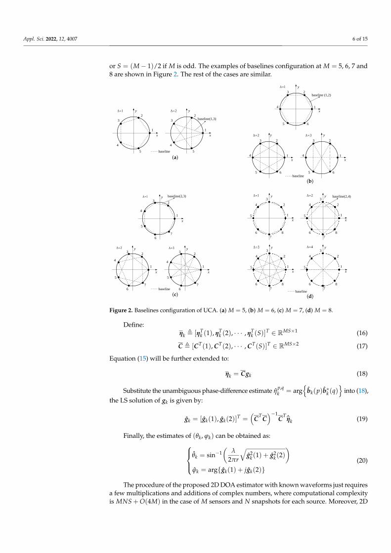
Consider the combination of all phase-difference equation sets corresponding todifferent sensor intervals ∆ = 1, 2, · · · , S, where S = M/2 if the sensor number M is even,

Appl. Sci. 2022, 12, 4007 6 of 15

or S = (M− 1)/2 if M is odd. The examples of baselines configuration at M = 5, 6, 7 and8 are shown in Figure 2. The rest of the cases are similar.

x

y

1

2

3

4

5 baseline

x

y

1

2

3

4

5

baseline(1,3)

2=1=

(a)x

y

1

23

4

5 6

x

y

1

23

4

5 6

x

y

1

23

4

5 6

baseline (1,2)

1=

2= 3=

baseline

(b)

x

2

5

6

3

4

1

7

y

baseline

x

2

5

6

3

4

1

7

y

x

2

5

6

3

4

1

7

y baseline(2,3)

2= 3=

1=

(c)

2

5

6

3

4

1

7

y

8

x

2

5

6

3

4

1

7

y

8

x

2

5

6

3

4

1

7

y

baseline

8

x

2

5

6

3

4

1

7

y

8

x

baseline(2,4)1= 2=

3= 4=

(d)

Figure 2. Baselines configuration of UCA. (a) M = 5, (b) M = 6, (c) M = 7, (d) M = 8.

Define:ηk , [ηT

k (1), ηTk (2), · · · , ηT

k (S)]T ∈ RMS×1 (16)

C , [CT(1), CT(2), · · · , CT(S)]T ∈ RMS×2 (17)

Equation (15) will be further extended to:

ηk = Cgk (18)

Substitute the unambiguous phase-difference estimate ηp,qk = arg

bk(p)b∗k (q)

into (18),

the LS solution of gk is given by:

gk = [gk(1), gk(2)]T =

(CTC

)−1CT

ηk (19)

Finally, the estimates of (θk, ϕk) can be obtained as:θk = sin−1(

λ

2πr

√g2

k (1) + g2k (2)

)ϕk = arggk(1) + jgk(2)

(20)

The procedure of the proposed 2D DOA estimator with known waveforms just requiresa few multiplications and additions of complex numbers, where computational complexityis MNS + O(4M) in the case of M sensors and N snapshots for each source. Moreover, 2D

Appl. Sci. 2022, 12, 4007 7 of 15

DOA estimates of K sources can be acquired separately and in parallel at the same time;hence, it is computationally efficient and easy to implement in practice.

4. Cramér-Rao Bound Derivation and Analysis

CRB is a theoretical lower bound for the covariance of any unbiased estimation.Therefore, it often serves as a benchmark to verify whether an algorithm achieves theoptimal performance [36–39]. In this section, we shall give the CRB of 2D DOA estimationfor signals without known waveforms from the previous works and derive the CRB withknown waveforms, respectively.

According to [24,39], CRB of 2D DOA estimation for signals without known wave-forms and unknown complex amplitudes, which is often referred as unconditional orstochastic CRB, is given by:

CRBu(ω) =σ2

v2N

[Re

H PT+

]−1∈ C2K×2K (21)

where ω = [θT ,ϕT ]T , H is defined as:

H , DH[

I − A(

AH A)−1

AH]

D ∈ C2K×2K (22)

D ,

[Dθ , Dϕ

]∈ CM×2K

Dθ ,[

a′θ1(θ1, ϕ1), a′θ2

(θ2, ϕ2), · · · , a′θk(θK, ϕK)

]∈ CM×K

Dϕ ,[

a′ϕ1(θ1, ϕ1), a′ϕ2

(θ2, ϕ2), · · · , a′ϕK(θK, ϕK)

]∈ CM×K

(23)

a′θ(θk, ϕk) ,

∂a(θk, ϕk)

∂θk=

[∂a1(θk, ϕk)

∂θk,

∂a2(θk, ϕk)

∂θk· · · ,

∂aM(θk, ϕk)

∂θk

]T∈ CM×1

a′ϕ(θk, ϕk) ,∂a(θk, ϕk)

∂ϕk=

[∂a1(θk, ϕk)

∂ϕk,

∂a2(θk, ϕk)

∂ϕk· · · ,

∂aM(θk, ϕk)

∂ϕk

]T∈ CM×1

(24)

P+ is defined as:

P+ ,[

PAH R−1 AP PAH R−1 APPAH R−1 AP PAH R−1 AP

]∈ C2K×2K (25)

where R and P are the array and signal covariance matrix, respectively:

R , E

x(t)xH(t)= lim

N→∞

1N

N

∑t=1

x(t)xH(t) = APAH + σ2v I ∈ CM×M (26)

P , E

s(t)sH(t)= lim

N→∞

1N

N

∑t=1

s(t)sH(t) ∈ CK×K (27)

CRB of 2D DOA estimation for signals with known waveforms and unknown complexamplitudes is a generalization of a similar result in [40] as:

CRBd(ω) =[Ω− Re

[U V

]HW−1[U V]]−1

∈ C2K×2K (28)

where Ω is defined as:

Ω ,2Nσ2

vRe(DH D) PT

−

∈ C2K×2K (29)

P− ,[

P PP P

]∈ C2K×2K (30)

Appl. Sci. 2022, 12, 4007 8 of 15

U, V and W are defined as:

U ,2σ2

v

N

∑t=1

SH(t)AH DθS(t) =2Nσ2

v(AH Dθ) PT ∈ CK×K

V ,2σ2

v

N

∑t=1

SH(t)AH DϕS(t) =2Nσ2

v(AH Dϕ) PT ∈ CK×K

W ,2σ2

v

N

∑t=1

SH(t)AH AS(t) =2Nσ2

v(AH A) PT ∈ CK×K

(31)

S(t) , diags(t) = diags1(t), s2(t), · · · , sK(t) ∈ CK×K

Y(t) , diagy(t) = diagy1(t), y2(t), · · · , yK(t) ∈ CK×K(32)

The derivation details are shown in the Appendix A.Here, we will provide some insights into CRBd(ω). If the source signals are un-

correlated with each other, i.e., P = diagσ2s1, σ2

s2, · · · , σ2sK is a diagonal matrix, where

σ2sk = E

|sk(t)|2

is the power of sk(t), (28) for UCA will reduce to:

CRBd(θk, ϕk) =σ2

v

2Nσ2sk

Re−1

[a′θk

(θk, ϕk)a′θk(θk, ϕk) 0

0 a′ϕk(θk, ϕk)a′ϕk

(θk, ϕk)

]=

λ2σ2v

4MNπ2r2σ2sk

diag−1cos2(θk), sin2(θk)

, k = 1, 2, · · · , K(33)

as a′θk

H(θk, ϕk)a′ϕk(θk, ϕk) = 0, a′θk

H(θk, ϕk)a(θk, ϕk) = 0 and a′ϕkH(θk, ϕk)a(θk, ϕk) = 0.

That is to say, in such a case, the CRB of any one of multiple sources is the same as the CRBwhen it is the only source. Hence, the CRB of 2D DOA estimation of different sources areindependent with each other and can be calculated separately. That also means that 2DDOA estimation performance will not degrade as the number of sources increases if thesource signals are uncorrelated with each other.

5. Simulation Results and Analysis

In this section, several simulations are carried out to validate the performance andefficiency of the proposed method. All the simulations were performed using MatlabR2018a on the Mac OS Monterey platform with an Intel i7 9750H CPU@2.6 GHz and 16 GBof RAM. We consider that there are three far-field narrowband signals impinging on aUCA with r/λ = 1/4 from (41.91, −68.92), (53.68, 71.97) and (47.56, 135.28). Thesignals and noise are both zero-mean complex white Gaussian sequences. Without loss ofgenerality, powers of the source signals are identical and powers of known waveforms arenormalized to unit. The unknown amplitude γ is assumed to be a random complex: realparts are determined by signal-to-noise ratio (SNR), and the imaginary parts lie randomlyin [0, 2π).

Four simulations were designed to investigate influence of different parameters on2D DOA estimation performance, i.e., SNR, number of sensors M, number of snapshots Nand correlation coefficient of signals. The source signals are assumed to be uncorrelatedwith each other in the first three simulations except the last one. In each simulation, theproposed interferometer-based estimator with known waveforms, the ML estimator withknown waveforms and the multi-direction virtual array transformation algorithm (MVATA)without known waveforms [41] are presented for performance comparison along withthe unconditional CRB and the CRB with known waveforms. For brevity, these termsare abbreviated as “Interferometer with KW”, “ML with KW”, “MVATA without KW”,“CRBu” and “CRBd” in the following figures and table. To evaluate the performance of theestimators , root mean squared error (RMSE) of azimuth and elevation angle estimation at

Appl. Sci. 2022, 12, 4007 9 of 15

each point in the following figures are measured from 2000 independent Monte Carlo runs,which is calculated as:

RMSE(θ) =√

E(θ1 − θ1)2 + (θ2 − θ2)2 + (θ3 − θ3)2

(34)

and RMSE(ϕ) is defined similarly. In addition, scatter plots of 2D DOA estimates of theproposed method are also depicted for each simulation.

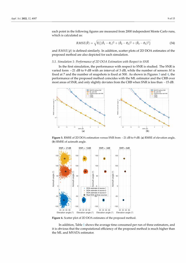
5.1. Simulation 1: Performance of 2D DOA Estimation with Respect to SNR

In the first simulation, the performance with respect to SNR is studied. The SNR isvaried form −21 dB to 9 dB with an interval of 3 dB, while the number of sensors M isfixed at 7 and the number of snapshots is fixed at 500. As shown in Figures 3 and 4, theperformance of the proposed method coincides with the ML estimator and the CRB overmost areas of SNR, and only slightly deviates from the CRB when SNR is less than −15 dB.

-20 -15 -10 -5 0 5

SNR (dB)

100

101

RM

SE

of

ele

va

tio

n a

ng

le (

°)

MVATA without KW

ML with KW

Interferometer with KW

CRBu

CRBd

(a)

-20 -15 -10 -5 0 5

SNR (dB)

100

101

RM

SE

of

azim

uth

an

gle

(°)

MVATA without KW

ML with KW

Interferometer with KW

CRBu

CRBd

(b)

Figure 3. RMSE of 2D DOA estimation versus SNR from −21 dB to 9 dB. (a) RMSE of elevation angle,(b) RMSE of azimuth angle.

20 40 60 80

Elevation angle (°)

-100

-50

0

50

100

150

Azim

uth

angle

(°)

SNR = -21dB

20 40 60 80

Elevation angle (°)

-100

-50

0

50

100

150

Azim

uth

angle

(°)

SNR = -12dB

20 40 60 80

Elevation angle (°)

-100

50

100

150

Azim

uth

angle

(°)

SNR = -3dB

20 40 60 80

Elevation angle (°)

-100

-50

0

50

100

150

Azim

uth

angle

(°)

SNR = 6dB

0DOA estimate of source 1 DOA estimate of source 2 DOA estimate of source 3 Real DOA of three sources -50

Figure 4. Scatter plot of 2D DOA estimates of the proposed method.

In addition, Table 1 shows the average time consumed per run of three estimators, andit is obvious that the computational efficiency of the proposed method is much higher thanthe ML and MVATA estimator.

Appl. Sci. 2022, 12, 4007 10 of 15

Table 1. Average time consumed per run of the three estimators.

Estimator MVATA without KW ML with KW Interferometer with KW

Time consumed 18.4 ms 34.5 ms 0.59 ms

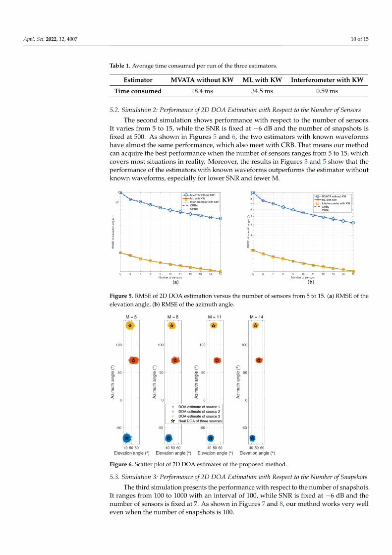
5.2. Simulation 2: Performance of 2D DOA Estimation with Respect to the Number of Sensors

The second simulation shows performance with respect to the number of sensors.It varies from 5 to 15, while the SNR is fixed at −6 dB and the number of snapshots isfixed at 500. As shown in Figures 5 and 6, the two estimators with known waveformshave almost the same performance, which also meet with CRB. That means our methodcan acquire the best performance when the number of sensors ranges from 5 to 15, whichcovers most situations in reality. Moreover, the results in Figures 3 and 5 show that theperformance of the estimators with known waveforms outperforms the estimator withoutknown waveforms, especially for lower SNR and fewer M.

5 6 7 8 9 10 11 12 13 14 15

Number of sensors

101

RM

SE

of

ele

va

tio

n a

ng

le (

°)

MVATA without KW

ML with KW

Interferometer with KW

CRBu

CRBd

(a)

5 6 7 8 9 10 11 12 13 14 15

Number of sensors

2

3

4

5

6

7

8

9

RM

SE

of

azim

uth

an

gle

(°)

MVATA without KW

ML with KW

Interferometer with KW

CRBu

CRBd

(b)

Figure 5. RMSE of 2D DOA estimation versus the number of sensors from 5 to 15. (a) RMSE of theelevation angle, (b) RMSE of the azimuth angle.

40 50 60

Elevation angle (°)

-50

0

50

100

Azim

uth

angle

(°)

M = 5

40 50 60

Elevation angle (°)

-50

0

50

100

Azim

uth

angle

(°)

M = 8

40 50 60

Elevation angle (°)

-50

0

50

100

Azim

uth

angle

(°)

M = 11

40 50 60

Elevation angle (°)

-50

0

50

100

Azim

uth

angle

(°)

M = 14

DOA estimate of source 1 DOA estimate of source 2 DOA estimate of source 3 Real DOA of three sources

Figure 6. Scatter plot of 2D DOA estimates of the proposed method.

5.3. Simulation 3: Performance of 2D DOA Estimation with Respect to the Number of Snapshots

The third simulation presents the performance with respect to the number of snapshots.It ranges from 100 to 1000 with an interval of 100, while SNR is fixed at −6 dB and thenumber of sensors is fixed at 7. As shown in Figures 7 and 8, our method works very welleven when the number of snapshots is 100.

Appl. Sci. 2022, 12, 4007 11 of 15

100 200 300 400 500 600 700 800 900 1000

Number of snapshots

101

RM

SE

of

ele

va

tio

n a

ng

le (

°)

MVATA without KW

ML with KW

Interferometer with KW

CRBu

CRBd

(a)

100 200 300 400 500 600 700 800 900 1000

Number of snapshots

101

RM

SE

of

azim

uth

an

gle

(°)

MVATA without KW

ML with KW

Interferometer with KW

CRBu

CRBd

(b)

Figure 7. RMSE of DOA estimation versus the number of snapshots from 100 to 1000. (a) RMSE ofthe elevation angle, (b) RMSE of the azimuth angle.

40 60

Elevation angle(°)

-50

0

50

100

150

Azim

uth

angle

(°)

N = 100

40 60

Elevation angle(°)

-50

0

50

100

150

Azim

uth

angle

(°)

N = 400

40 60

Elevation angle(°)

-50

0

50

100

150

Azim

uth

angle

(°)

N = 700

40 60

Elevation angle(°)

-50

0

50

100

150

Azim

uth

angle

(°)

N = 1000

DOA estimate of source 1 DOA estimate of source 2 DOA estimate of source 3 Real DOA of three sources

Figure 8. Scatter plot of 2D DOA estimates of the proposed method.

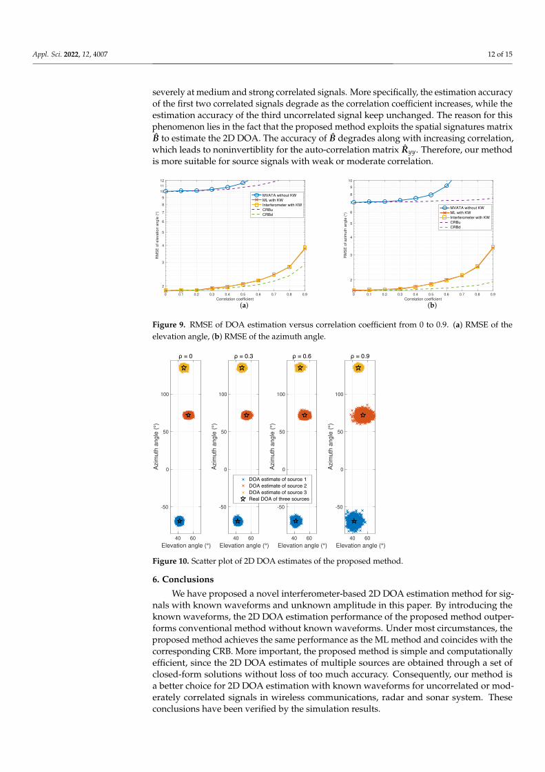
5.4. Simulation 4: Performance of 2D DOA Estimation with Respect to Correlation Coefficient

The last simulation inspects the performance against correlation between signals. Weassume the first two signals are correlated and the third signal is uncorrelated with the firsttwo. Under this assumption, the signal covariance matrix P is:

P =

σ2s ρσ2

s 0ρ∗σ2

s σ2s 0

0 0 σ2s

(35)

where σ2s is the power of the three signals and ρ is the correlation coefficient of the first two

signals, which is defined as:

ρ =Es1(t)s∗2(t)√

E|s1(t)|2E|s2(t)|2= lim

N→∞

1σ2

s

N

∑t=1

s1(t)s∗2(t) (36)

In this simulation, the correlation coefficient of the first two signals is varied from 0to 0.9, while SNR is fixed at −6 dB, the number of sensors is fixed at 7 and the numberof snapshots is fixed at 500. As shown in Figures 9 and 10, performance of the proposedmethod approaches to the CRB for weak and moderately correlated signals but degrades

Appl. Sci. 2022, 12, 4007 12 of 15

severely at medium and strong correlated signals. More specifically, the estimation accuracyof the first two correlated signals degrade as the correlation coefficient increases, while theestimation accuracy of the third uncorrelated signal keep unchanged. The reason for thisphenomenon lies in the fact that the proposed method exploits the spatial signatures matrixB to estimate the 2D DOA. The accuracy of B degrades along with increasing correlation,which leads to noninvertiblity for the auto-correlation matrix Ryy. Therefore, our methodis more suitable for source signals with weak or moderate correlation.

0 0.1 0.2 0.3 0.4 0.5 0.6 0.7 0.8 0.9

Correlation coefficient

2

3

4

5

6

7

8

9

10

11

12

RM

SE

of

ele

va

tio

n a

ng

le (

°)

MVATA without KW

ML with KW

Interferometer with KW

CRBu

CRBd

(a)

0 0.1 0.2 0.3 0.4 0.5 0.6 0.7 0.8 0.9

Correlation coefficient

2

3

4

5

6

7

8

9

10

RM

SE

of

azim

uth

an

gle

(°)

MVATA without KW

ML with KW

Interferometer with KW

CRBu

CRBd

(b)

Figure 9. RMSE of DOA estimation versus correlation coefficient from 0 to 0.9. (a) RMSE of theelevation angle, (b) RMSE of the azimuth angle.

40 60

Elevation angle (°)

-50

0

50

100

Azim

uth

angle

(°)

40 60

Elevation angle (°)

-50

0

50

100

Azim

uth

angle

(°)

40 60

Elevation angle (°)

-50

0

50

100

Azim

uth

angle

(°)

40 60

Elevation angle (°)

-50

0

50

100

Azim

uth

angle

(°)

DOA estimate of source 1 DOA estimate of source 2 DOA estimate of source 3 Real DOA of three sources

Figure 10. Scatter plot of 2D DOA estimates of the proposed method.

6. Conclusions

We have proposed a novel interferometer-based 2D DOA estimation method for sig-nals with known waveforms and unknown amplitude in this paper. By introducing theknown waveforms, the 2D DOA estimation performance of the proposed method outper-forms conventional method without known waveforms. Under most circumstances, theproposed method achieves the same performance as the ML method and coincides with thecorresponding CRB. More important, the proposed method is simple and computationallyefficient, since the 2D DOA estimates of multiple sources are obtained through a set ofclosed-form solutions without loss of too much accuracy. Consequently, our method isa better choice for 2D DOA estimation with known waveforms for uncorrelated or mod-erately correlated signals in wireless communications, radar and sonar system. Theseconclusions have been verified by the simulation results.

Appl. Sci. 2022, 12, 4007 13 of 15

Moreover, our method does not perform well for medium- or strong-correlated signals.Some possible further works may consider addressing the above problem as well asevaluating of theoretical lower bound on RMSE of the proposed method and extending theinterferometer-based method to other planar arrays, such as uniform rectangular array orL-shape array.

Author Contributions: Conceptualization, Z.H. and Q.W. (Qun Wan); methodology, Z.H., J.Z. andQ.W. (Qi Wu); software, Z.H.; validation, Z.H. and Q.W. (Qi Wu); writing—original draft preparation,Z.H.; writing—review and editing, Z.H., Q.W. (Qi Wu), J.Z. and Q.W. (Qun Wan). All authors haveread and agreed to the published version of the manuscript.

Funding: This research was supported in part by the National Natural Science Foundation of China (NSFC)under Grant 61771108, National Science and technology major project under Grant 2016ZX03001022 andthe Foundation of Sichuan Science and Technology Project under Grant 18ZDYF0990.

Institutional Review Board Statement: Not applicable.

Informed Consent Statement: Not applicable.

Data Availability Statement: The data used to support the findings of this study are included withinthe article.

Conflicts of Interest: The authors declare no conflict of interest.

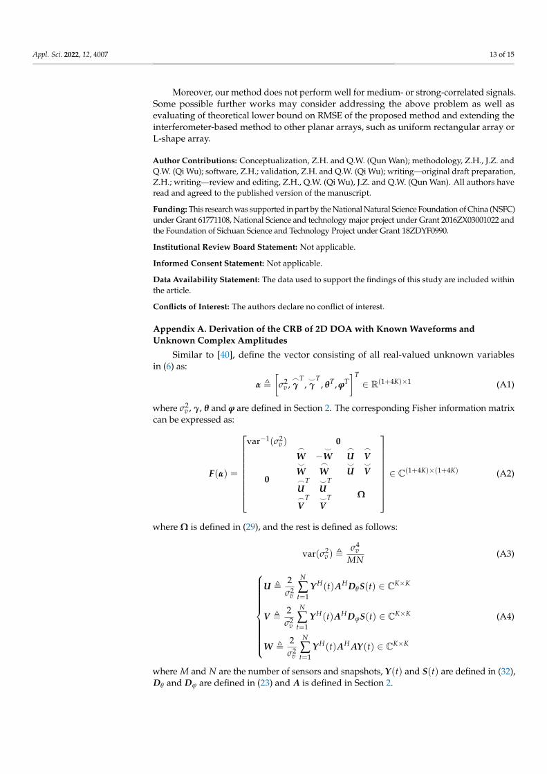
Appendix A. Derivation of the CRB of 2D DOA with Known Waveforms andUnknown Complex Amplitudes

Similar to [40], define the vector consisting of all real-valued unknown variablesin (6) as:

α ,[

σ2v ,

_γ

T,^γ

T, θT ,ϕT

]T∈ R(1+4K)×1 (A1)

where σ2v , γ, θ and ϕ are defined in Section 2. The corresponding Fisher information matrix

can be expressed as:

F(α) =

var−1(σ2v ) 0

0

_W −

^W

^W

_W

_U

_V

^U

^V

_U

T ^U

T

_V

T ^V

T Ω

∈ C(1+4K)×(1+4K) (A2)

where Ω is defined in (29), and the rest is defined as follows:

var(σ2v ) ,

σ4v

MN(A3)

U ,2σ2

v

N

∑t=1

Y H(t)AH DθS(t) ∈ CK×K

V ,2σ2

v

N

∑t=1

Y H(t)AH DϕS(t) ∈ CK×K

W ,2σ2

v

N

∑t=1

Y H(t)AH AY(t) ∈ CK×K

(A4)

where M and N are the number of sensors and snapshots, Y(t) and S(t) are defined in (32),Dθ and Dϕ are defined in (23) and A is defined in Section 2.

Appl. Sci. 2022, 12, 4007 14 of 15

Given the relationship between CRB and the Fisher information matrix [31], CRB forω = [θT ,ϕT ]T with known waveforms and unknown complex amplitudes is:

CRBd(ω) =

Ω−

_U

T ^U

T

_V

T ^V

T

[_W −

^W

^W

_W

]−1[_U

_V

^U

^V

]−1

=

Ω− Re[

U V]HW−1[U V

]−1

(A5)

As we can see from (A4) and (A5), CRB seems like a function of yk(t)Kk=1 and γ, and

varies along them. To reduce CRB to a fixed expression independent of them, substituterelationship U = Γ−HU, V = Γ−HV and W = Γ−HWΓ−1 into (A5), where Γ is defined inSection 2, U, V and W are defined in (31) and CRB can be further simplified to (28).

References1. Krim, H.; Viberg, M. Two decades of array signal processing research: The parametric approach. IEEE Signal Process Mag. 1996,

13, 67–94. [CrossRef]2. Trees Van, H.L. Detection, Estimation, and Modulation Theory, Optimum Array Processing; John Wiley & Sons, Inc.: New York, NY,

USA, 2004.3. Capon, J. High-resolution frequency-wavenumber spectrum analysis. Proc. IEEE 1969, 57, 1408–1418. [CrossRef]4. Schmidt, R. Multiple emitter location and signal parameter estimation. IEEE Trans. Antennas Propag. 1986, 34, 276–280. [CrossRef]5. Roy, R.; Kailath, T. ESPRIT-estimation of signal parameters via rotational invariance techniques. IEEE Trans. Acoust. Speech Signal

Process. 1989, 37, 984–995. [CrossRef]6. Stoica, P.; Sharman, K. Maximum likelihood methods for direction-of-arrival estimation. IEEE Trans. Acoust. Speech Signal Process.

1990, 38, 1132–1143. [CrossRef]7. Malioutov, D.; Cetin, M.; Willsky, A. A sparse signal reconstruction perspective for source localization with sensor arrays. IEEE

Trans. Signal Process. 2005, 53, 3010–3022. [CrossRef]8. Yang, Z.; Xie, L.; Zhang, C. Off-Grid Direction of Arrival Estimation Using Sparse Bayesian Inference. IEEE Trans. Signal Process.

2013, 61, 38–43. [CrossRef]9. Kim, J.M.; Lee, O.K.; Ye, J.C. Compressive MUSIC: Revisiting the Link Between Compressive Sensing and Array Signal Processing.

IEEE Trans. Inf. Theory 2012, 58, 278–301. [CrossRef]10. Li, J.; Compton, R. Maximum likelihood angle estimation for signals with known waveforms. IEEE Trans. Signal Process. 1993,

41, 2850–2862. [CrossRef]11. Li, J.; Halder, B.; Stoica, P.; Viberg, M. Computationally efficient angle estimation for signals with known waveforms. IEEE Trans.

Signal Process. 1995, 43, 2154–2163. [CrossRef]12. Cedervall, M.; Moses, R. Efficient maximum likelihood DOA estimation for signals with known waveforms in the presence of

multipath. IEEE Trans. Signal Process. 1997, 45, 808–811. [CrossRef]13. Li, H.; Pu, H.; Li, J. Efficient maximum likelihood angle estimation for signals with known waveforms in white noise. In

Proceedings of the Ninth IEEE Signal Processing Workshop on Statistical Signal and Array Processing, Portland, OR, USA,14–16 September 1998; pp. 25–28. [CrossRef]

14. Najjar Atallah, L.; Marcos, S. DOA estimation and association of coherent multipaths by using reference signals. Signal Process.2004, 84, 981–996. [CrossRef]

15. Wang, N.; Agathoklis, P.; Antoniou, A. A new DOA estimation technique based on subarray beamforming. IEEE Trans. SignalProcess. 2006, 54, 3279–3290. [CrossRef]

16. Gu, J.F.; Wei, P.; Tai, H.M. Fast direction-of-arrival estimation with known waveforms and linear operators. IET Signal Proc. 2008,2, 27–36. [CrossRef]

17. Emadi, M.; Sadeghi, K.H. DOA Estimation of Multi-Reflected Known Signals in Compact Arrays. IEEE Trans. Aerosp. Electron.Syst. 2013, 49, 1920–1931. [CrossRef]

18. Gu, J.F.; Zhu, W.P.; Swamy, M.N.S. Sparse linear arrays for estimating and tracking DOAs of signals with known waveforms.In Proceedings of the 2013 IEEE International Symposium on Circuits and Systems (ISCAS), Beijing, China, 199–23 May 2013;pp. 2187–2190. [CrossRef]

19. Gu, J.F.; Zhu, W.P.; Swamy, M. Fast and efficient DOA estimation method for signals with known waveforms using nonuniformlinear arrays. Signal Process. 2015, 114, 265–276. [CrossRef]

20. Dong, Y.Y.; Dong, C.X.; Liu, W.; Liu, M.M.; Tang, Z.Z. Robust DOA Estimation for Sources With Known Waveforms AgainstDoppler Shifts via Oblique Projection. IEEE Sens. J. 2018, 18, 6735–6742. [CrossRef]

21. Dong, Y.Y.; Dong, C.X.; Liu, W.; Liu, M.M. DOA estimation with known waveforms in the presence of unknown time delays andDoppler shifts. Signal Process. 2020, 166, 107232. [CrossRef]

Appl. Sci. 2022, 12, 4007 15 of 15

22. Wax, M.; Adler, A. Localization of multiple sources with known waveforms by array response matching. Signal Process. 2020,177, 107721. [CrossRef]

23. Dong, Y.Y.; Dong, C.X.; Liu, W.; Cai, J. Generalized l2-lp minimization based DOA estimation for sources with known waveformsin impulsive noise. Signal Process. 2022, 190, 108313. [CrossRef]

24. Mathews, C.; Zoltowski, M. Eigenstructure techniques for 2-D angle estimation with uniform circular arrays. IEEE Trans. SignalProcess. 1994, 42, 2395–2407. [CrossRef]

25. Wei, H.; Shi, Y. Performance analysis and comparison of correlative interferometers for direction finding. In Proceedings of the2010 IEEE 10th International Conference on Signal Processing Proceedings, Beijing, China, 24–28 October 2010; pp. 393–396.[CrossRef]

26. Liao, B.; Wu, Y.T.; Chan, S.C. A Generalized Algorithm for Fast Two-Dimensional Angle Estimation of a Single Source withUniform Circular Arrays. IEEE Antennas Wirel. Propag. Lett. 2012, 11, 984–986. [CrossRef]

27. Liu, Z.M.; Guo, F.C. Azimuth and Elevation Estimation With Rotating Long-Baseline Interferometers. IEEE Trans. Signal Process.2015, 63, 2405–2419. [CrossRef]

28. He, C.; Chen, J.; Liang, X.; Geng, J.; Zhu, W.; Jin, R. High-Accuracy DOA Estimation Based on Time-Modulated Array with Longand Short Baselines. IEEE Antennas Wirel. Propag. Lett. 2018, 17, 1391–1395. [CrossRef]

29. Sadeghi, M.; Behnia, F.; Haghshenas, H. Positioning of Geostationary Satellite by Radio Interferometry. IEEE Trans. Aerosp.Electron. Syst. 2019, 55, 903–917. [CrossRef]

30. Hu, Z.; Wan, Q. Enhanced Interferometer DOA Estimator for Signal with Known Waveform. In Proceedings of the 2019 11thInternational Conference on Wireless Communications and Signal Processing (WCSP), Xi’an, China, 23–25 October 2019; pp. 1–5.[CrossRef]

31. Kay, S.M. Fundamentals of Statistical Signal Processing: Estimation Theory; Prentice-Hall, Inc.: Hoboken, NJ, USA, 1993.32. Zoltowski, M.; Mathews, C. Real-time frequency and 2-D angle estimation with sub-Nyquist spatio-temporal sampling. IEEE

Trans. Signal Process. 1994, 42, 2781–2794. [CrossRef]33. Sundaram, K.; Mallik, R.; Murthy, U. Modulo conversion method for estimating the direction of arrival. IEEE Trans. Aerosp.

Electron. Syst. 2000, 36, 1391–1396. [CrossRef]34. Wu, Y.; So, H.C. Simple and Accurate Two-Dimensional Angle Estimation for a Single Source with Uniform Circular Array. IEEE

Antennas Wirel. Propag. Lett. 2008, 7, 78–80. [CrossRef]35. Xin, J.; Liao, G.; Yang, Z.; Shen, H. Ambiguity Resolution for Passive 2-D Source Localization with a Uniform Circular Array.

Sensors 2018, 18, 2650. [CrossRef]36. Stoica, P.; Nehorai, A. MUSIC, maximum likelihood, and Cramer-Rao bound. IEEE Trans. Acoust. Speech Signal Process. 1989,

37, 720–741. [CrossRef]37. Stoica, P.; Nehorai, A. MUSIC, maximum likelihood, and Cramer-Rao bound: Further results and comparisons. IEEE Trans.

Acoust. Speech Signal Process. 1990, 38, 2140–2150. [CrossRef]38. Stoica, P.; Nehorai, A. Performance study of conditional and unconditional direction-of-arrival estimation. IEEE Trans. Acoust.

Speech Signal Process. 1990, 38, 1783–1795. [CrossRef]39. Stoica, P.; Larsson, E.; Gershman, A. The stochastic CRB for array processing: A textbook derivation. IEEE Signal Process Lett.

2001, 8, 148–150. [CrossRef]40. Li, J. Array Signal Processing for Polarized Signals and Signals with Known Waveforms. Ph.D. Thesis, The Ohio State University,

Columbus, OH, USA, 1991.41. Xu, J.; Nie, K.; Feng, Z.; Chen, J.; Fang, Y. A multi-direction virtual array transformation algorithm for 2D DOA estimation. Signal

Process. 2016, 125, 122–133. [CrossRef]