1

A Dynamical Systems Analysis of Methanol-Air Auto-Ignition

1R.D. Lockett,

2G.N. Robertson

1School of Engineering and Mathematical Sciences, The City University,

Northampton Square, London, EC1V 0HB, United Kingdom.

2Department of Physics, University of Cape Town, Rondebosch 7700,

Republic of South Africa.

Corresponding Author: R.D. Lockett

Email: r.d.lockett@city.ac.uk

Tel. 44 (0) 207 040 8812

Fax. 44 (0) 207 040 8566

2

Abstract

Dynamical systems analysis was employed as an alternative investigative tool

to conventional reaction path analysis and sensitivity analysis in methanol-air auto-

ignition, in which the non-linear chemical rate equations describing a homogeneous,

methanol-air auto-ignition system were linearised. The resultant system of linear,

inhomogeneous differential equations were solved analytically using an eigen-mode

analysis. The numerically determined solution to the non-linear auto-ignition

trajectory was employed to determine the local analytic behaviour for a number of

regular points along the solution trajectory to equilibrium. The solution trajectory was

found to qualitatively change three times, thereby defining four different regions in the

time and temperature domain. The dominant eigen-mode solutions were expressed in

terms of dominant reactions at regular intervals along the solution path, revealing the

dominant local chemistry. The solution trajectory was dominated by four explosive

modes in the first, low temperature region (T < 1090 K). Two dominant explosive

modes coupled to form an explosive, oscillating mode in the second region (1090 K <

T < 1160 K). In the third region (1160 K < T < 2000 K), the explosive, oscillating

mode changed to a decaying, oscillating mode. The changes in the low temperature

region of the solution trajectory were found to be associated with the critical points in

the evolution of the branching agent (hydrogen peroxide) concentration. The third

qualitative change occurred at T ~ 2000 K, when the dominant decaying, oscillating

mode describing methanol and formaldehyde oxidation to carbon monoxide collapsed,

to be replaced with real, decaying modes (proper stable nodes) describing the wet

oxidation of carbon monoxide to carbon dioxide, and its reverse reaction, together

with the high temperature formation of water and other equilibrium products.

3

Keywords

Dynamical Systems Analysis, Auto-ignition, Bifurcation, Chemical Kinetics, Eigen-

mode Analysis, Chemical Explosion, Branching, Thermal Explosion.

4

1. Introduction

It is a common practice in the study of systems of non-linear differential

equations to linearise the set of equations about various points along the solution

trajectory (usually in the neighbourhood of a local equilibrium point), and then,

wherever possible, solve for the linearised system. These linearised solutions are then

first order approximations to the true solution of the problem, and are generally used

to study the qualitative behaviour of the non-linear system at the specified points along

the solution trajectory. This approach forms the basis of a dynamical systems analysis

of a non-linear dynamical system [1, 2].

Furthermore, the linearised mathematical solution at regular points along the

solution trajectory of a real, non-linear dynamical system can be decomposed into

terms of real eigen-modes or complex conjugate pairs of eigen-modes. The full linear

solution can then be expressed in terms of a sum of one- and two-dimensional eigen-

mode solutions. The eigen-modes have eigenvalues that are either real and positive

(explosive modes), real and negative (decaying modes), complex with positive real

parts (explosive, oscillatory modes), complex with negative real parts (decaying,

oscillatory modes), or imaginary.

Several methods of dynamical systems analysis have been employed in

theoretical and numerical research in combustion. K. Chinnick et al [3] used a

linearisation technique in studying oscillatory reaction behaviour in H2/O2 systems.

This study was conducted analytically using a simplified H2/O2 reaction mechanism.

They were able to derive explicit expressions defining the critical ignition boundary

criteria and the conditions for oscillatory ignition.

5

On the other hand, Maas and Pope [4] have used qualitative dynamical

methods as a means of determining how flame chemical kinetics can be simplified.

They showed that the linearised time development of flame chemistry can be closely

approximated by a subspace of the composition space, where the subspace is defined

as that in which all movements of the chemistry correspond to slower time scales.

This subspace is determined by finding the points in the composition space that are in

equilibrium with respect to the fastest time scales of the chemical system. The linear

analysis was then generalised to the full non-linear problem. They were able to

demonstrate the method successfully for a CO/H2/air system, reducing the system to

one and two-dimensional manifolds in the reaction space, and comparing the results

with conventional reduced mechanisms. Maas, Pope and others have since applied

this technique to chemical mechanism reduction in complex flame chemistry

successfully [5 – 8].

The Computational Singular Perturbation (CSP) method of mechanism

analysis and reduction has been developed by Lam and Goussis [9 – 11]. This method

involves utilizing the eigenvectors obtained from the diagonalisation of the linearised

rate equation Jacobian as a preferred set of basis vectors to identify the fast chemistry

manifold (near-equilibrium processes), and the slow chemistry manifold (time-

dependent processes) imbedded in the solution manifold. The eigenvalues obtained

from the diagonal Jacobian define the different time scales associated with the

chemical kinetic solution trajectory, and are employed to discriminate between the

slow chemistry manifold and the fast chemistry manifold. The eigenvectors associated

with the slow manifold are then used to determine the tangent space to the slow

chemistry manifold. The tangent space is then employed to achieve the reduction of

6

the chemical mechanism. The methodology has been further developed, refined, and

employed by them and others [12 – 14].

As a result, the methods of dynamical systems analysis are often employed in

the canonical reduction of combustion mechanisms. However, the methodology can

also be employed to provide new insights into the evolution of chemically explosive

combustion systems, to be used, either together with, or as an alternative to, reaction

path analysis and sensitivity analysis. Natural applications of this methodology

include explosion limits, ignition processes, engine auto-ignition and HCCI

combustion.

The mathematical method presented here is very similar to that of the original

work of Maas and Pope [4], and Lam and Goussis [9], but was developed

independently of them, at around the same time [15]. The fundamental difference

between this analysis, and that of Maas and Pope, is that this was developed in order to

provide a new and alternative insight into chemically explosive systems. The

expectation was that, in a chemically explosive system described by branching, only a

small number of independent eigen-modes would dominate the solution trajectory.

Low temperature chemical branching and high temperature recombination is of central

importance in understanding auto-ignition, and can then be understood in terms of the

development of these eigen-modes, rather than in terms of a numerical solution to a

large system of coupled reaction equations. Dynamical systems analysis of auto-

ignition is expected to provide a more intuitive explanation of chemical branching,

propagation and equilibrium termination than conventional reaction path analysis

(RPA) and/or sensitivity analysis (SA), which will be discussed in detail later.

Section 2 contains a presentation of a number of standard methods employed in

the analysis of combustion mechanisms. These include the quasi-steady state

7

approximation (QSSA), the method of partial equilibrium (PEA), reaction path

analysis (RPA), and sensitivity analysis (SA). Section 2 is provided in order to

contrast the results of dynamical systems analysis with the more conventional methods

of chemical mechanism analysis.

In addition to the other conventional methods of mechanism analysis (Quasi-

Steady State Approximation (QSSA), Partial Equilibrium Assumption (PEA), RPA,

and SA), high activation energy asymptotic analysis has been employed successfully

in the course of investigating the basic structure of flames subject to single step

chemistry [16, 17], the detailed structure of the relatively cool induction region of

hydrogen-oxygen detonation waves [18], and a number of other combustion

applications [19, 20].

The dynamical systems analysis contained in this paper was applied to the

modeling study of methanol auto-ignition in a methanol-fuelled internal combustion

engine performed by Driver et al. [21]. The physical model to be explored was how

the cylinder end-gas (the unburned mixture ahead of the flame front) had its enthalpy

raised by cylinder and flame front compression, and heat transfer, until auto-ignition,

followed by a comprehensive examination of the branching and thermal chemistry

involved in auto-ignition.

The explosive chemical system subjected to analysis was a homogeneous

methanol/air mixture subjected to a measured, temperature-pressure-volume history

until shortly before the mixture became explosive. Following the last of the

temperature measurements, the mixture was assumed to be subject to adiabatic

compression until and through the calculated chemical and thermal explosion. For the

experimental details of the temperature and pressure measurements in the engine, the

8

reader should refer to reference [22], and for the modeling details of the auto-ignition

chemistry, the reader should refer to references [21] and [23].

2. An Introduction to Mechanism Analysis

2.1 Quasi-Steady State Approximation (QSSA)

A simple reaction sequence, consisting of two elementary reaction steps, will

be employed to illustrate the quasi-steady state approximation. The reaction sequence

DCBAkk

+→→21

, (A)

subject to initial conditions [A](t0) = A0, [B](t0) = 0, [C](t0) = 0, and [D](t0) = 0, has an

exact analytic solution for the time-dependent species concentrations:

[A](t) = A0( )01 ttk

e−− , (1)

[B](t) = A0( ) ( )( )0102

21

1 ttkttkee

kk

k −−−− −−

, (2)

[C](t) = [D](t) = A0

( ) ( )

−+

−−

−−−−

21

2

21

10102

1kk

ek

kk

ekttkttk

. (3)

If it is now assumed that species B is very reactive in forming C and D (k2 >>

k1), then the rate of consumption of species B is approximately equal to the rate of

formation of species B. This condition defines the quasi-steady state approximation,

which is then expressed as

9

0][][][

21 ≈−= BkAkdt

Bd. (4)

Solving for [B](t), [C](t), and [D](t) produces the solutions

[B](t) =( )01

2

01 ttke

k

Ak −−, (5)

[C](t) = [D](t) = A0( )( )011

ttke

−−− . (6)

A comparison of the exact solutions and the approximate solutions obtained

using the quasi-steady state approximation above shows that the approximate solution

is obtained directly from the exact solution when k2 >> k1, and t – t0 >> 1/k2.

A classic example of the application of the quasi-steady state approximation

which is widely taught in combustion courses involves the derivation of the overall

reaction rate for the oxidation of hydrogen in bromine to form hydrogen bromide [24,

25].

The proposed mechanism for the oxidation of hydrogen in bromine is

Br2 + M 1k

→ Br + Br + M (B)

Br + H2 2k

→ HBr + H (C)

H + HBr 3k

→ Br + H2 (D)

H + Br2 4k

→ HBr + Br (E)

Br + Br + M 5k

→ Br2 + M (F)

Using the quasi-steady state assumption, the rate laws for the intermediates H and Br

are

10

[ ] [ ][ ] [ ][ ] [ ][ ] [ ] [ ]

[ ] [ ][ ] [ ][ ] 0]][[

02]][[2

24322

2

52224321

≈−−=

≈−−++=

BrHkHBrHkHBrkdt

Hd

MBrkHBrkBrHkHBrHkMBrkdt

Brd

(7)

Therefore [ ] [ ][ ][ ]243

22

][ BrkHBrk

HBrkH

+= . Summation of these two equations produces

[ ] [ ]

5

21

k

BrkBr = . Hence the rate law for the formation of hydrogen bromide is

[ ] [ ][ ] [ ][ ]

[ ][ ]

][

][1

2

]][[

24

3

2

5

212

32422

Brk

HBrk

Hk

Brkk

HBrHkBrHkHBrkdt

HBrd

+

=−+= (8)

2.2 Partial Equilibrium Assumption (PEA)

An example of the partial equilibrium assumption can be found in high

temperature hydrogen-oxygen combustion (T > 2000K) [26]. A modern hydrogen-

oxygen combustion mechanism can be employed to show that the following forward

and reverse reactions

H + O2 ⇔1

2

k

k

OH + O (F)

O + H2 ⇔3

4

k

k

OH + H (G)

H2 + OH ⇔5

6

k

k

H2O + H (H)

are very fast at high temperatures (T > 2000K). Under these conditions, a partial

equilibrium is said to exist for these three reactions. Hence

11

k1[H][O2] = k2[OH][O] (9)

k3[H2][O] = k4[OH][H] (10)

k5[H2][OH] = k6[H2O][H]. (11)

The intermediate species concentrations can then be expressed in terms of the major

species concentrations:

]][[][

][

]][[][

][

][][][

22

42

31

262

2251

2

2

2

642

2

3

2

2

531

OHkk

kkOH

OHkk

OHkkO

OHkkk

OHkkkH

=

=

=

. (12)

2.3 Reaction Path Analysis (RPA)

During the numerical integration of a set of rate equations in order to obtain the

solution trajectory, the mechanism itself can be subjected to a local analysis in order to

discover the relationship between individual reactions and the rate of formation and

consumption of the active chemical species. This analysis constitutes the basis for a

local reaction path analysis [26].

The results of the local reaction path analysis are normally presented in the

form of a table, providing the relative rates of formation and consumption of species

by the reactions constituting the mechanism. The table is normally determined for

each point along the solution trajectory. Table 1 below shows the format of such a

table, and the type of information provided.

12

(Please insert Table 1 here.)

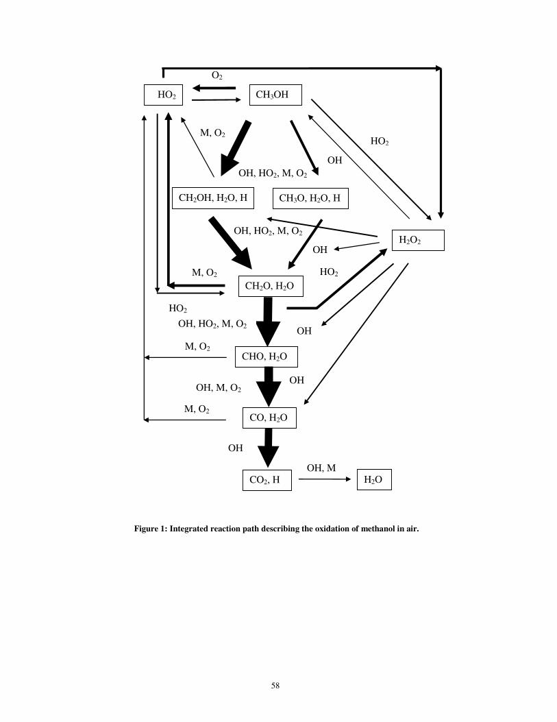
Integrating the local reaction path over the time domain from initiation to

completion defines an integral or global reaction path analysis [26]. This analysis

provides the dominant reaction paths for the entire combustion process under

investigation. The results of an integral path analysis are normally presented in the

form of a flowchart. Figure 1 shows such a flowchart, indicating the reaction flow for

the explosive oxidation of methanol in air, initiated from an intermediate temperature

(T ~ 1,100 K).

(Please insert Figure 1 here.)

2.4 Sensitivity Analysis (SA)

The chemical rate law describing the rate of change of concentration of chemical

species with time, temperature and pressure, can be expressed in vector form in the

following way:

dt

dy(t) = A(T).y + B(T):yy + C(T)�yyy, (13)

where y(t) is the species concentration vector, and A(T), B(T), and C(T) are two-

dimensional, three dimensional, and four dimensional matrices respectively,

containing in turn molecular fission reaction rate coefficients, bi-molecular collision

rate coefficients, and termolecular collision rate coefficients.

13

Suppose that a number of reaction rate coefficients describing reactions

comprising the combustion mechanism are ill-defined (this is usually the case in fully

detailed combustion mechanisms). Sensitivity analysis of the combustion mechanism

aims to provide quantitative information on the relative dependence of species

concentrations on reaction rate coefficients. Applying sensitivity analysis to a

combustion mechanism enables the determination of the dominant elementary

reactions determining the solution trajectory.

The relative sensitivity of the i’th species concentration (yi) to a variation in

reaction rate coefficient kj for the j’th reaction is defined by Sij [27], where

j

i

j

i

i

j

ijk

y

k

y

y

kS

ln

ln

∂

∂=

∂

∂= . (14)

As an example, this definition of the relative sensitivity will be applied to the

simple reaction sequence discussed in Section 2.1 above (Reaction Sequence A). The

relative sensitivity of species 3 (species C) to reaction rate coefficients k1 and k2 is

then given by

( )( )[ ]

( )( )[ ]tktk

tktk

eetkkkkC

kkAS

eetkkkkC

kkAS

12

21

1)(][

1)(][

212

21

21032

122

21

210

31

−−

−−

+−−−

=

+−−−

=

. (15)

Following on from the above example (k2 >> k1), S31 → 1 as t → ∞, and S32 → 0 as

t → ∞. This result identifies that the product species C has a large relative sensitivity

14

to the slow, rate limiting reaction rate of A → B, and small relative sensitivity to the

fast reaction rate of B → C + D.

Figure 2 shows the relative sensitivity of the various species involved in the

auto-ignition of methanol in air, taken from reference [21].

(Please insert Figure 2 here.)

3. Derivation of the Linear Mode Analysis

The system of reaction equations are linearised in the following way. The

species concentration vector y(t) has vector elements denoted by yi (t), i ∈ [1,2,3,…N],

where N is the number of atomic and molecular species in the complete chemical

mechanism. y(t) evolves according to the system of equations

dt

dy(t) = A(T).y + B(T):yy + C(T)�yyy. (16)

The two-dimensional matrix A contains temperature dependent rate

coefficients for all of the uni-molecular decomposition reactions in the mechanism.

The matrix elements of A are denoted by Aij, i,j ∈ [1, 2, 3,…N]. The three-

dimensional matrix B contains temperature dependent rate coefficients for all of the

bimolecular reactions in the mechanism. The matrix elements of B are denoted by Bijk,

i,j,k ∈ [1, 2, 3,…N]. The four-dimensional matrix C contains temperature dependent

rate coefficients for all of the termolecular reactions in the mechanism. The matrix

elements of C are denoted by Cijkl, i,j,k,l ∈ [1, 2, 3, …N].

15

If the species concentration solution vector y(t) is expanded about some regular

point in the solution trajectory y (t0), then the concentration displacement vector from

that regular point x (t) can be defined as x (t) = y (t) – y (t0).

The equation for x (t) can be expressed in terms of the i’th element of the

vector, which is given by

( ) ( )( )

( )( )( )∑∑∑

∑∑∑

= = =

= ==

++++

++++=

N

j

N

k

llkkjj

N

l

ijkl

kk

N

j

N

k

jjijkjj

N

j

ij

i

tyxtyxtyxC

tyxtyxBtyxAdt

dx

1 1

000

1

0

1 1

00

1

)()()(

)()()(

(17)

The non-linear terms in equation (17) above involve sums over the product terms xjxk

and xjxkxl.

Equation (17) is linearised by ignoring terms that are quadratic and cubic in the

concentration displacement vector x. This yields the linearised equation for the i’th

component of the vector x.

( )[ ] ( )[ ]j

N

j

N

k

N

l

lkilkjikjlijklj

N

j

N

k

kikjijk

N

j

jij

lkj

N

j

N

k

N

l

ijklk

N

j

N

k

jijk

N

j

jij

i

i

xtytyCCCxtyBBxA

tytytyCtytyBtyAdt

dxx

∑∑∑∑∑∑

∑∑∑∑∑∑

= = == ==

= = == ==

++++++

++==

1 1 1

00

1 1

0

1

000

1 1 1

00

1 11

0

)()()(

)()()()()()(�

(18)

Equation (18) can be re-written in a simpler form

∑=

+=N

jjijii xKMx

1

� (19)

16

Equation (19) can be expressed in vector form

dt

d x = K. x + M. (20)

An alternative formulation of the problem expressed above can be obtained

through a Taylor series expansion of the concentration vector y (t) about a regular

point in the trajectory y (t0).

dt

dy (t) = A(T).y + B(p,T):yy + C(p,T)�yyy = f (y). (21)

The local behaviour of the concentration vector y (t) in the neighborhood of a

regular point in the trajectory y (t0) can be determined by approximating the vector f in

the neighborhood of y (t0). The first order approximation is

f (y0 + dy) = f (y0) + K.dy (22)

where K is the Jacobian matrix obtained from f (y) [4]. The first order approximation

leads to the linear differential equations above (equations (19) and (20)).

Equations (19) and (20) define a system of coupled first order linear

differential equations, with initial conditions x (t0) = 0. As long as the matrix K can be

diagonalised, the general solution for equation (20) above is

x (t) = Q . e γ )( 0tt −

. C – Q . γγγγ -1

.Q -1

.M (23)

17

where Q is the matrix of eigenvectors of matrix K, γγγγ is a diagonal matrix with the

diagonal elements given by the eigenvalues of matrix K, and e γ )( 0tt −

is the

diagonal matrix

e γ )( 0tt − =

−

−

−

����

....00

....00

....00

)(

)(

)(

03

02

01

tt

tt

tt

e

e

e

γ

γ

γ

(24)

It is believed that the linearised matrix K, derived from a realistic, detailed

chemical mechanism where all elements of the matrix are real, and all species

concentrations are linearly independent of all other species concentrations, is

diagonalizable at all regular points along the solution trajectory except at the final

equilibrium point, and the eigenvalues of K remain distinct.

Applying the initial conditions yields the exact solution

x (t) = Q . (e γ )( 0tt −

– δδδδ ) . γγγγ -1

.Q -1

.M (25)

The linearised solution for x (t) is in the form of an eigenvalue-eigenvector

decomposition of matrix K, involving the vector M.

In order to find the projection of the solution vector x (t) onto the eigenvectors,

we write

x (t) = Q . a (t) (26)

18

a (t) is the time dependent projection of the solution vector x (t) onto the eigenvectors,

and is found by pre-multiplying the above equation by Q -1

to give

a (t) = Q -1

. x (t) (27)

yielding

a (t) = (e γ )( 0tt −

– δδδδ ) . γγγγ -1

.Q -1

.M (28)

Mathematical systems of this sort are dynamic in the sense that the linearised

solution derived above reflects not only the reaction chemistry, but also the response

of the system to changes in the state variables, such as temperature, pressure and

volume. A study of the evolution of the eigenvalues, eigenvectors and consequent

solution vector therefore provides important information on the qualitative behaviour

of the system. The dominant modes of the system are those whose rates of production

of species are largest.

In mathematical systems of this kind, the eigen-mode solutions that dominate

the solution trajectory may abruptly change their analytic behaviour. The system is

then said to have undergone a bifurcation at this point. This change in analytic

behaviour reveals a qualitative change in the evolution of the system. Bifurcations are

identified as follows: no functional mapping exists to map the form of the solution

prior to the bifurcation to the solution after the bifurcation. Pseudo-bifurcations occur

when the solutions change structure, but a functional mapping can be found to map the

solution prior to the pseudo-bifurcation to the solution after the pseudo-bifurcation.

19

By examining closely the detailed mechanism around the bifurcation and

pseudo-bifurcation points, the reasons for the bifurcations, and hence the source of the

corresponding change in the chemistry, can be revealed.

Eigen-mode rates of formation and consumption at regular points along the

solution trajectory are derivable from Equation (28) in the form

c (t) = dt

da (t) = Q

-1(t).M (t) (29)

The eigen-mode rates of formation and consumption for the i’th chemical species in

the system can be expressed in the form ∑ −=j

jiji tMtQtc )()()( 1 .

4. Programming Features

The original modeling was performed on a personal computer, using Warnatz's

HOMREACT program [28], based on Deuflhard's numerical integrator LIMEX [29].

The modeling was performed using a core set of 188 reactions involving 21 chemical

species extracted from the mechanism proposed by Grotheer et al [23]. This

mechanism was employed to calculate the methanol/air auto-ignition process, which

was then compared against the auto-ignition calculation involving the full mechanism

[21]. There were no significant differences found. Furthermore, for purposes of

comparison, the analysis presented here was repeated using the Norton and Dryer

mechanism [30], and the later Held and Dryer mechanism [31]. There were no

significant differences regarding the predicted auto-ignition trajectories obtained from

the various mechanisms, nor the mathematical behaviour of the various solutions.

20

A FORTRAN program called CHEMMODE was written to calculate

numerical expressions for x (t) and a (t). The output of HOMREACT includes local

concentrations, temperatures, pressures, rate coefficients, and reaction stoichiometric

coefficients at regular points along the solution trajectory. CHEMMODE reads in this

data, prepares the Jacobian matrix K and the vector M, and then diagonalises K. The

elements of K are all real. Therefore, the eigenvalues and eigenvector elements must

be real, or complex conjugate pairs, in order for x (t) to have real elements.

The routine used to diagonalise the Jacobian matrix K first balanced the matrix,

followed by a similarity transformation to upper Hessenberg form, analogous to

Gaussian elimination with pivoting. The routine then used a QR algorithm with shifts

and Gaussian elimination with pivoting to find the eigenvalues and eigenvectors

respectively.

5. Eigen-Mode Analysis of Methanol/Air Auto-ignition

5.1 Preliminary Remarks

This section discusses the mathematical structure of the dominant eigen-modes

along the solution trajectory of the methanol-air auto-ignition system, and the

chemistry that results. In the following analysis, the eigen-mode rates of formation

and consumption are presented as forward reactions with the relevant elements of the

eigenvectors altered to achieve a normalized unit stoichiometric coefficient for the

most important reactant. These reactions (derived from the eigenvectors) form the

basis for a rigorous decomposition and analysis of the auto-ignition system. The γi

represent the eigenvalues of the dominant eigen-modes presented, and the ci are the

21

rates of production of species associated with the specified eigen-mode at time t0, and

are given by ∑ −=j

jiji MQc1 .

Figure 3 shows the evolution of the major species and the temperature during

auto-ignition. Figure 4 shows the evolution of the intermediate species and the

temperature during auto-ignition. The three bifurcations are shown on the graphs

occurring at the times specified by the three vertical lines crossing the time axis.

(Please insert Figure 3 here.)

(Please insert Figure 4 here.)

5.2 Eigen-Mode Analysis

In summary, the solution trajectory of the auto-ignition system bifurcates three

times during the course of the reaction. During the first part of the branching reaction,

the dominant eigen-modes are unstable nodes. The first bifurcation occurs at the point

of inflection of the hydrogen peroxide concentration-time curve. This is shown in

Figure 3 and Figure 4 as the first vertical line crossing the time axis at t = 0.9500 ms.

This is not surprising, as hydrogen peroxide serves as the degenerate branching agent

for the system. The two dominant explosive modes couple together to form an

explosive, oscillating mode. This marks the point on the solution trajectory where the

meta-stable hydrogen peroxide begins to thermally decompose to hydroxyl radicals,

thereby branching, and accelerating exothermic oxidation (thermal runaway).

The second qualitative change in the trajectory occurs when the hydrogen

peroxide concentration nears its maximum value. This is shown in Figure 3 and

22

Figure 4 as the dotted line crossing the time axis at t = 0.9730 ms. At this point, the

dominant eigen-modes change from an unstable focus to a stable focus. This marks

the point where the rate of thermal decomposition of hydrogen peroxide to hydroxyl

radicals is greater than the rate of formation, and the beginning of the thermal

explosion of the methanol-air mixture.

The third bifurcation occurs at approximately 2000 K, when the dominant

decaying, oscillating mode disappears, to be replaced by real, evanescent eigen-modes.

This is shown in Figure 3 and Figure 4 as the solid vertical line crossing the time axis

at t = 0.9849 ms. The dominant stable focus describing methanol and formaldehyde

oxidation to carbon monoxide is replaced with two real eigen-modes describing the

oxidation of carbon monoxide to carbon dioxide, and the reverse reaction.

Appendix 1 shows the eigen-mode eigenvectors that dominate the solution

trajectory from the beginning of the auto-ignition process at approximately 1000 K,

through to the chemical equilibrium formed at the adiabatic flame temperature of

approximately 2 600K.

Figure 5 shows the magnitude of the rate of formation associated with the

dominant eigen-modes as a function of temperature through the auto-ignition from

initiation to equilibrium. At the low temperature initiation of auto-ignition, the real

eigen-mode describing methanol oxidation dominates the solution trajectory

(eigenvector 1), accompanied by its reverse reaction (eigenvector 2). As the

temperature rises, so does the concentration of carbon monoxide. This rise is

accompanied by a growing carbon monoxide oxidation reaction to carbon dioxide

(eigenvector 3). As the temperature reaches 2000 K, the methanol and formaldehyde

burn out, causing a collapse of the dominant eigen-mode. Wet carbon monoxide

23

oxidation to carbon dioxide suddenly dominates the auto-ignition path to equilibrium,

accompanied by its reverse reaction.

(Please insert Figure 5 here.)

Figure 6 shows the evolution of the eigenvalues of the dominant, coupled

complex eigen-modes displayed in the complex plane as a function of temperature up

to 1900 K. As the temperature rises above 1900 K, the methanol and formaldehyde

burns out, causing the dominant eigen-modes to collapse, to be replaced with the real,

evanescent eigen-modes describing wet CO oxidation to CO2, and the reverse reaction

describing CO2 reduction back to CO. Figure 7 shows the real, negative eigenvalues

for the other dominant eigen-modes, including that associated with wet CO oxidation

to CO2, and the reverse reduction reaction.

(Please insert Figure 6 here.)

(Please insert Figure 7 here.)

5.2.1 1000 K < T < 1090K

5.2.1.1. T = 1008 K, P = 36.09 bar

At this temperature and pressure, the solution is dominated by four real eigen-

modes (> 95 % of formation and consumption of major species). An approximate

local solution for the n’th element of x (p, T, t) can be expressed as

24

for the four real, independent modes. The xn(t) are the elements of the vector

x (p, T, t), while λmn refers to the n vector elements of the m’th eigenvector. γm refers

to the m’th eigenvalue, and cm refers to the rate of production of species for the m’th

eigen-mode.

The approximate solution for the eigen-mode rates c (p, T, t) are obtained from

the eigenvectors presented in Appendix 1, and can be expressed in reaction form,

which is described by

(1.1.1) CH3OH + 0.644 O2 → 0.958 CH2O + 0.810 H2O + 0.181 H2O2 + 0.042 CO

γ1 = 5029 s-1

, c1 = 1 499 mole.m-3

.s-1

(1.1.2) CH2O + 0.008 CO2 + 0.546 H2O → 0.768 CH3OH + 0.240 CO + 0.256 O2 +

0.016 H2O2

γ2 = - 704 s-1

, c2 = 441 mole.m-3

.s-1

(1.1.3) CO2 + 0.374 CO + 0.069 CH2O + 2.770 H2O + 0.006 CH4 + 0.044 H2 → 1.448

CH3OH + 1.884 O2

γ3 = 8.2 s-1

, c3 = 122.0 mole.m-3

.s-1

(1.1.4) CO + 0.192 CH3OH + 0.025 CH2O + 0.727 O2 → 1.210 CO2 + 0.249 H2O +

0.145 H2 + 0.007 CH4

( ) ( ) ( )

( )4

44)(

3

33)(

2

22)(

1

11)(

1

111),,(

04

030201

γ

λ

γ

λ

γ

λ

γ

λ

γ

γγγ

ntt

nttnttntt

n

ce

ce

ce

cetTpx

−

+−+−+−≈

−

−−−

25

γ4 = - 18.1 s-1

, c4 = 148.6 mole.m-3

.s-1

The dominant mode (reaction 1.1.1) is an explosive mode with a reaction time-

scale of 0.20 ms, involving the exothermic oxidation of methanol to form

formaldehyde, water, and the degenerate branching agent hydrogen peroxide. The

second important eigen-mode (reaction 1.1.2) describes an endothermic reverse

reaction between formaldehyde and water, to form methanol, oxygen, and importantly,

more hydrogen peroxide.

5.2.1.2 T = 1028 K, P = 39.16 bar

At this temperature and pressure, the four dominant modes remain (> 95% of

formation and consumption of major species). The first, and most important, is just an

evolution of the dominant explosive mode from above. The second dominant mode

combines the reverse reaction with formaldehyde oxidation to CO. The third mode

describes an endothermic reverse reaction of CO2, CO and formaldehyde to methanol.

The fourth mode describes the exothermic oxidation of carbon monoxide to carbon

dioxide.

(1.2.1) CH3OH + 0.649 O2 → 0.862 CH2O + 0.136 CO + 0.002 CO2 + 0.954 H2O +

0.142 H2O2 + 0.029 HO2 + 0.028 H2

γ1 = 5 561 s-1

, c1 = 6 918 mole.m-3

.s-1

(1.2.2) CH2O + 0.619 H2O + 0.009 H2 + 0.006 CO2 → 0.792 CH3OH + 0.215 CO +

0.263 O2 + 0.041 H2O2

26

γ2 = - 2 474 s-1

, c2 = 925.0 mole.m-3

.s-1

(1.2.3) CO2 + 0.553 CO + 0.091 CH2O + 0.010 CH4 + 3.145 H2O → 1.654 CH3OH +

2.069 O2

γ3 = 41.1 s-1

, c3 = 587.7 mole.m-3

.s-1

(1.2.4) CO + 0.655 O2 + 0.096 CH3OH + 0.012 CH2O + 0.042 H2 → 1.096 CO2 +

0.011 CH4 + 0.222 H2O + 0.001 H2O2

γ4 = - 67.6 s-1

, c4 = 523.6 mole.m-3

.s-1

5.2.1.3 T = 1048 K, P = 41.34 bar

As the temperature of the system reaches 1048 K, the system is qualitatively

described by a three-mode solution, which is of the form

for three real, independent eigen-modes. Qualitatively, the system is three-

dimensional in nature, dominated by the first mode discussed above. The locus of

regular points in this part of the trajectory of the system is a locus of explosive, real

modes. The eigen-mode rates of formation and consumption are expressed in reaction

form.

(1.3.1) CH3OH + 0.714 O2 → 0.703 CH2O + 0.288 CO + 0.009 CO2 + 1.122 H2O +

0.128 H2O2 + 0.021 HO2 + 0.036 H2

( ) ( ) ( )3

33)(

2

22)(

1

11)(111),,( 030201

γ

λ

γ

λ

γ

λ γγγ nttnttntt

n

ce

ce

cetTpx −+−+−≈ −−−

27

γ1 = 6 892 s-1

, c1 = 22 495 mole.m-3

.s-1

(1.3.2) CO2 + 0.937 CO + 0.129 CH2O + 0.016 CH4 + 3.922 H2O + 0.008 H2O2 →

2.078 CH3OH + 2.463 O2

γ2 = 186.7 s-1

, c2 = 2 218 mole.m-3

.s-1

(1.3.3) CO + 0.075 CH3OH + 0.010 CH2O + 0.60 O2 + 0.016 H2 → 1.069 CO2 +

0.015 CH4 + 0.141 H2O + 0.002 H2O2

γ3 = - 176.9 s-1

, c3 = 1 885 mole.m-3

.s-1

5.2.1.4. T = 1071 K, P = 42.70 bar

(1.4.1) CH3OH + 0.799 O2 → 0.511 CH2O + 0.462 CO + 0.026 CO2 + 1.322 H2O +

0.109 H2O2 + 0.016 HO2 + 0.049 H2

γ1 = 8239 s-1

, c1 = 65 722 mole.m-3

.s-1

(1.4.2) CO + 0.576 CO2 + 0.131 CH2O + 0.010 CH4 + 3.185 H2O + 0.019 H2O2 →

1.717 CH3OH + 1.898 O2

γ2 = 725.5 s-1

, c2 = 12 743 mole.m-3

.s-1

(1.4.3) CO + 0.058 CH3OH + 0.008 CH2O + 0.565 O2 + 0.008 H2 → 1.048 CO2 +

0.018 CH4 + 0.093 H2O + 0.003 H2O2

γ3 = - 394.0 s-1

, c3 = 5 448 mole.m-3

.s-1

28

(1.4.4) CH3OH + 0.266 CO + 0.314 O2 + 0.099 H2O2 + 0.016 HO2 → 1.255 CH2O +

0.011 CO2 + 0.845 H2O + 0.007 H2

γ4 = - 11 560.0 s-1

, c4 = 3 645 mole.m-3

.s-1

As the temperature of the combustion system reaches 1088 K, the two

competing exponentially increasing modes that dominate the qualitative behaviour of

the system in this temperature regime are of similar importance, since the rates of

production of species from the two dominant modes are of opposite sign, and

approximately equal magnitude.

5.2.1.5. T = 1088 K, P = 43.26 bar

(1.5.1) CH3OH + 0.879 O2 → 0.336 CH2O + 0.604 CO + 0.059 CO2 + 1.517 H2O +

0.079 H2O2 + 0.012 HO2 + 0.059 H2

γ1 = 7 601 s-1

, c1 = 173 815 mole.m-3

.s-1

(1.5.2) CO + 0.313 CO2 + 0.174 CH2O + 0.005 CH4 + 2.674 H2O + 0.037 H2O2 →

1.492 CH3OH + 1.535 O2

γ2 = 2 232 s-1

, c2 = 66 470 mole.m-3

.s-1

(1.5.3) CO + 0.046 CH3OH + 0.007 CH2O + 0.542 O2 + 0.007 H2 → 1.034 CO2 +

0.019 CH4 + 0.061 H2O + 0.003 H2O2

γ3 = - 394.0 s-1

, c3 = 10 500 mole.m-3

.s-1

29

(1.5.4) CH3OH + 0.254 CO + 0.315 O2 + 0.111 H2O2 + 0.017 HO2 → 1.241 CH2O +

0.013 CO2 + 0.874 H2O + 0.004 H2

γ4 = - 11 560.0 s-1

, c4 = 8 350 mole.m-3

.s-1

5.2.2. 1090 K < T < 1170 K, 43.4 bar < P < 44.1 bar

In this temperature regime the two explosive modes that previously dominated

the auto-ignition trajectory couple together to form a complex conjugate pair with a

positive real part, defining a decaying, oscillating mode.

The evolving coupled modes are related to the onset of hydrogen peroxide

decomposition to hydroxyl radicals, and the consequent increase in methanol

oxidation. These reactions are exothermic, and the heat liberated is now sufficient to

heat the end-gas methanol/air mixture.

The change in the chemistry is reflected by the bifurcation in the trajectory of

the system, and, as pointed out earlier, occurs at the point of inflection of the hydrogen

peroxide concentration trajectory in time. In other words, the change in the structure

of the chemical rate equations occurs when the second time derivative of the hydrogen

peroxide concentration is zero. The point in time when the bifurcation occurs is

shown in Figures 2 and 3 by the first vertical line along the time axis, occurring at time

t = 0.9500 ms.

The rate of reaction associated with the explosive, oscillating mode is

approximately nine times larger than that of the next largest mode. Therefore, these

two coupled modes dominate the linear solution space of the chemical system. If the

eigenvalues of the coupled, exponentially increasing, oscillatory modes are γ + iω and

γ - iω respectively, the coupled two mode solution vector has the form

30

[ ]( )( )( )

[ ]( )( )( )ωγ

λλ

ωγ

λλλλ ωγωγ

i

iicce

i

iiccetatatx inrnirtiinrnirti

nnn−

−−−+

+

++−=+≈ −+ 11)()()( )()(

2211

where λrn and λin are the real and imaginary elements of the eigenvector λλλλ, cr and ci

are the time independent real and imaginary components of the projection of the

normalised eigenvector λλλλ onto the vector describing the rate of species production

dx/dt. This approximate solution for the elements of x can be re-expressed in the form

( ) ( ) ( )[ ] ( ) ( )[ ]2222

sin21cos2)(

ωγ

ωγλωγλω

ωγ

ωγλωγλω γγ

+

−++−

+

−−+−≈ rirnirin

t

riinirrn

t

n

cccctecccctetx

The elements of x (xn (t)) increase exponentially with a time dependence given by the

real part of γ, and simultaneously oscillates with frequency ω.

Examining the evolution of the complex eigenvalues reveals that the rate of

exponential increase decreases with time, and the frequency of oscillation increases

relative to the rate of exponential increase. The time scales defined by the dominant

complex eigenvalues and the evolution of the chemistry result in there not being

enough time for the system to pass through a single oscillation before a second

qualitative transition takes place. Chemically, this means that the net rate of

production of degenerate branching agent (hydrogen peroxide) in the methanol/air

oxidation system begins to decrease.

5.2.2.1. T = 1097 K, P = 43.45 bar

(2.1.1) CH3OH + 0.147 CO2 + 0.694 O2 → 0.568 CO + 0.581 CH2O + 1.195 H2O +

0.145 H2O2 + 0.073 H2 + 0.023 HO2

31

γ1 = 5 053 + 1439i s-1

, |c1| = 95 000 mole.m-3

.s-1

(2.1.2) CO + 0.040 CH3OH + 0.007 CH2O + 0.532 O2 → 1.028 CO2 + 0.019 CH4

+ 0.047 H2O + 0.004 H2O2

γ2 = - 828.8 s-1

, c2 = 14 100 mole.m-3

.s-1

(2.1.3) CH3OH + 0.245 CO + 0.318 O2 + 0.115 H2O2 + 0.018 HO2 → 1.231 CH2O +

0.891 H2O + 0.013 CO2 + 0.002 H2

γ3 = - 21 710 s-1

, c3 = 11 600 mole.m-3

.s-1

5.2.2.2. T = 1130 K, P = 43.85 bar

(2.2.1) CH3OH + 0.159 CO2 + 0.730 O2 + 0.003 CH4 → 0.724 CO + 0.439 CH2O +

1.331 H2O + 0.120 H2O2 + 0.105 H2 + 0.022 HO2

γ1 = 4 419 + 10 600i s-1

, |c1|= 2.00 x 105 mole.m

-3.s

-1

(2.2.2) CO + 0.023 CH3OH + 0.005 CH2O + 0.501 O2 → 1.009 CO2 + 0.020 CH4 +

0.006 H2 + 0.004 H2O2 + 0.003 H2O

γ2 = - 1 744 s-1

, c2 = 34 100 mole.m-3

.s-1

(2.2.3) CH3OH + 0.195 CO + 0.324 O2 + 0.127 H2O2 + 0.024 HO2 + 0.004 H2 →

1.179 CH2O + 0.963 H2O + 0.015 CO2

γ3 = - 41 700 s-1

, c3 = 29 300 mole.m-3

.s-1

32

5.2.2.3. T = 1165 K, P = 44.04 bar

(2.3.1) CH3OH + 0.168 CO2 + 0.745 O2 + 0.003 CH4 → 0.849 CO + 0.322 CH2O +

1.439 H2O + 0.148 H2 + 0.087 H2O2 + 0.021 HO2

γ1 = 116.8 + 23 100i s-1

, |c1|= 3.76 x 105 mole.m

-3.s

-1

(2.3.2) CO + 0.474 O2 + 0.035 H2O + 0.009 CH3OH + 0.002 CH2O → 0.992 CO2 +

0.019 CH4 + 0.013 H2 + 0.004 H2O2

γ2 = - 3356 s-1

, c2 = 71 600 mole.m-3

.s-1

(2.3.3) CH3OH + 0.120 CO + 0.368 O2 + 0.136 H2O2 + 0.032 HO2 + 0.007 H2 →

1.103 CH2O + 1.055 H2O + 0.016 CO2

γ3 = - 76 350 s-1

, c3 = 62 700 mole.m-3

.s-1

Reactions 2.3.1 and 2.3.2 are quasi-termination reactions in that they both

produce degenerate branching agent hydrogen peroxide. The reaction system is also

self-heating through the exothermic production of CH2O, H2O, CO, and CO2.

5.2.3. 1170 K < T < 2000 K, 44.1 bar < P < 44.6 bar

Thermal runaway begins at this stage of auto-ignition. Mathematically, the

dominant eigen-mode undergoes a pseudo-bifurcation from an unstable focus to a

stable focus. This change is a consequence of the coupled exponentially increasing,

oscillatory modes changing to coupled, exponentially decaying, oscillatory modes.

This means that the chemical system will now converge towards its equilibrium point,

33

along an inward spiral. As this transition takes place, other real evanescent modes are

introduced that are also important in the evolution of the system.

The pseudo-bifurcation from an explosive, oscillating mode to a decaying,

oscillating mode of the dominant eigen-mode occurs when hydrogen peroxide nears its

maximum concentration. In other words, the pseudo-bifurcation occurs in a

neighbourhood of the point when the first time derivative of the hydrogen peroxide

concentration is zero. This is shown by the second vertical line along the time axis in

Figures 2 and 3. This point can be used to define the beginning of thermal runaway.

Chemically, the system is now described in terms of a branching reaction

sequence. The intermediate chemical species (apart from hydrogen peroxide) quickly

reach their maximum concentrations, simultaneous with thermal explosion, through

the rapid oxidation of methanol by hydroxyl radicals and molecular oxygen to

formaldehyde and water, followed by the oxidation of formaldehyde to carbon

monoxide. The rapid release of heat into the gas mixture causes the temperature of the

gas to rise far more rapidly than the rate of increase of the external pressure.

Consequently, the gas expands rapidly, and the species concentrations decrease.

The exponentially decaying oscillatory modes reflect the chemically explosive

condition of the methanol/air oxidation system as explained earlier. The dominant

coupled complex eigen-modes explain the exothermic chemistry in terms of the

oxidation reactions of methanol to formaldehyde and water, followed by the oxidation

reactions of formaldehyde to carbon monoxide and water. The dominance of these

two coupled modes continues to about 2000 K, at which time the mode reflecting the

wet oxidation of carbon monoxide to carbon dioxide begins to take over, and

dominates the system in the thermally explosive regime 2000 K to equilibrium at

approximately 2600 K.

34

5.2.3.1 T = 1169 K, P = 44.06 bar

(3.1.1) CH3OH + 0.745 O2 + 0.170 CO2 → 0.865 CO + 0.307 CH2O + 1.451 H2O +

0.154 H2 + + 0.083 H2O2 + 0.020 HO2

γ1 = - 969.1 + 25 000i s-1

, |c1| = 4.02 x 105 mole.m

-3.s

-1

(3.1.2) CO + 0.471 O2 + 0.040 H2O + 0.007 CH3OH + 0.002 CH2O → 0.990 CO2 +

0.019 CH4 + 0.014 H2 + 0.004 H2O2 + 0.001 HO2

γ2 = - 3 617 s-1

, c2 = 77 900 mole.m-3

.s-1

(3.1.3) CH3OH + 0.109 CO + 0.371 O2 + 0.137 H2O2 + 0.033 HO2 + 0.007 H2 →

1.092 CH2O + 0.016 CO2 + 1.068 H2O

γ3 = - 82 010 s-1

, c3 = 67 700 mole.m-3

.s-1

Reaction 3.1.1 which evolves into reaction 3.2.1 below shows the transition of

the auto-ignition system through the net formation of degenerate branching agent

hydrogen peroxide (reaction 3.1.1) to the net consumption of hydrogen peroxide

(reaction 3.2.1).

5.2.3.2 T = 1294 K, P = 44.25 bar

(3.2.1) CH3OH + 0.649 O2 + 0.198 CO2 + 0.006 HO2 + 0.005 H2O2 → 1.514 H2O +

1.191 CO + 0.490 H2 + 0.009 CH2O

γ1 = - 104 100 + 96 560i s-1

, |c1| = 1.608 x 106 mole.m

-3.s

-1

35

(3.2.2) H2 + 0.338 CO + 0.329 O2 → 0.576 H2O + 0.148 CH3OH + 0.120 CH2O +

0.070 CO2 + 0.004 H2O2 + 0.003 HO2

γ2 = - 78 270 s-1

, c2 = 4.99 x 105 mole.m

-3.s

-1

(3.2.3) CO + 0.414 O2 + 0.121 H2O → 0.954 CO2 + 0.033 H2 + 0.024 CH3OH

+ 0.002 H2O2 + 0.002 HO2

γ3 = - 18 490 s-1

, c3 = 4.26 x 105 mole.m

-3.s

-1

(3.2.4) CH3OH + 0.524 O2 + 0.152 H2O2 + 0.109 HO2 → 1.552 H2O + 0.599 CH2O

+ 0.379 CO + 0.056 H2 + 0.022 CO2

γ4 = - 484 800 s-1

, c4 = 4.45 x 105 mole.m

-3.s

-1

Reactions 3.2.1 above and 3.3.1 below mark the temperature regime (1300 K <

T < 1400 K) where the formaldehyde concentration reaches its maximum value. For

larger temperatures (T > 1400K), formaldehyde is oxidized to carbon monoxide and

water.

Reactions 3.2.2 above and 3.3.2 below contain the reverse reaction to

Reactions 3.2.1 and 3.3.1, growing in magnitude with temperature. Reactions 3.2.3

above and 3.3.3 below are the reactions describing the exothermic oxidation of carbon

monoxide to carbon dioxide.

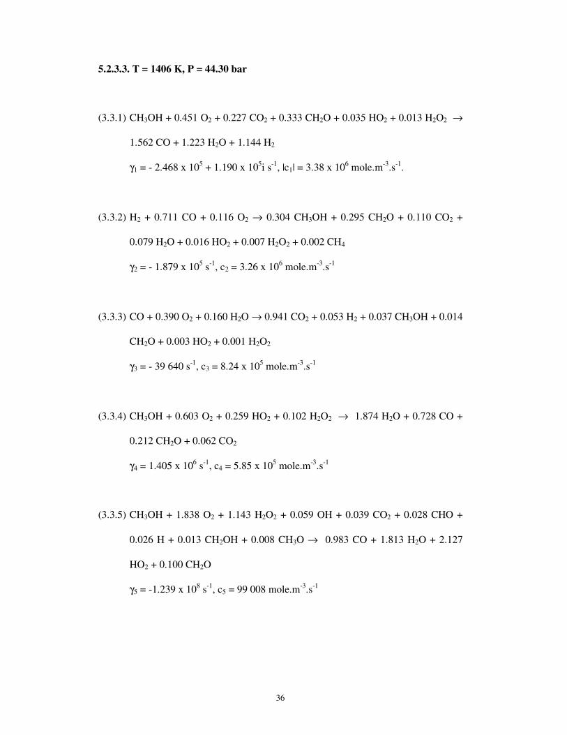
36

5.2.3.3. T = 1406 K, P = 44.30 bar

(3.3.1) CH3OH + 0.451 O2 + 0.227 CO2 + 0.333 CH2O + 0.035 HO2 + 0.013 H2O2 →

1.562 CO + 1.223 H2O + 1.144 H2

γ1 = - 2.468 x 105 + 1.190 x 10

5i s

-1, |c1| = 3.38 x 10

6 mole.m

-3.s

-1.

(3.3.2) H2 + 0.711 CO + 0.116 O2 → 0.304 CH3OH + 0.295 CH2O + 0.110 CO2 +

0.079 H2O + 0.016 HO2 + 0.007 H2O2 + 0.002 CH4

γ2 = - 1.879 x 105 s

-1, c2 = 3.26 x 10

6 mole.m

-3.s

-1

(3.3.3) CO + 0.390 O2 + 0.160 H2O → 0.941 CO2 + 0.053 H2 + 0.037 CH3OH + 0.014

CH2O + 0.003 HO2 + 0.001 H2O2

γ3 = - 39 640 s-1

, c3 = 8.24 x 105 mole.m

-3.s

-1

(3.3.4) CH3OH + 0.603 O2 + 0.259 HO2 + 0.102 H2O2 → 1.874 H2O + 0.728 CO +

0.212 CH2O + 0.062 CO2

γ4 = 1.405 x 106 s

-1, c4 = 5.85 x 10

5 mole.m

-3.s

-1

(3.3.5) CH3OH + 1.838 O2 + 1.143 H2O2 + 0.059 OH + 0.039 CO2 + 0.028 CHO +

0.026 H + 0.013 CH2OH + 0.008 CH3O → 0.983 CO + 1.813 H2O + 2.127

HO2 + 0.100 CH2O

γ5 = -1.239 x 108 s

-1, c5 = 99 008 mole.m

-3.s

-1

37

5.2.3.4. T = 1548 K, P = 44.34 bar

(3.4.1) CH3OH + 0.846 O2 + 0.827 CH2O + 0.081 CO2 + 0.062 HO2 + 0.005 H2O2 →

1.906 CO + 1.910 H2O + 0.947 H2

γ1 = - 3.062 x 105 + 2.089 x 10

5i s

-1, |c1| = 4.62 x 10

6 mole.m

-3.s

-1

(3.4.2) CO + 0.746 H2 + 0.476 H2O → 0.700 CH2O + 0.252 CH3OH + 0.178 O2 +

0.048 CO2 + 0.033 HO2 + 0.003 H2O2

γ2 = - 5.706 x 105 s

-1, c2 = 4.26 x 10

6 mole.m

-3.s

-1

(3.4.3) CO + 0.344 O2 + 0.238 H2O → 0.920 CO2 + 0.100 H2 + 0.053 CH3OH + 0.024

CH2O + 0.005 HO2 + 0.003 CH4

γ3 = - 64 740 s-1

, c3 = 1.12 x 106 mole.m

-3.s

-1

5.2.3.5 T= 1689 K, P = 44.36 bar

(3.5.1) CH3OH + 1.054 O2 + 0.777 CH2O + 0.046 HO2 + 0.001 H2O2 → 1.743 CO +

2.198 H2O + 0.565 H2

γ1 = - 4.904 x 105 + 7.411 x 10

5i s

-1, |c1| = 6.168 x 10

6 mole.m

-3.s

-1

(3.5.2) CO + 0.889 H2 + 0.113 CH3OH + 0.048 O2 → 1.069 CH2O + 0.041 CO2 +

0.038 H2O + 0.009 HO2 + 0.003 CHO + 0.002 CH4

γ2 = - 1.998 x 106 s

-1, c2 = 1.770 x 10

6 mole.m

-3.s

-1

38

(3.5.3) CO + 0.386 O2 + 0.202 H2O + 0.019 CH4 + 0.002 CH3 → 0.949 CO2 + 0.123

H2 + 0.046 CH3OH + 0.025 CH2O

γ3 = - 1.067 x 105 + 1.074 x 10

5i s

-1, |c3| = 1.642 x 10

6 mole.m

-3.s

-1

(3.5.4) H2O + 0.460 CO + 0.059 H2 + 0.080 CO2 + 0.026 CH4 → 0.443 CH3OH +

0.374 O2 + 0.152 HO2 + 0.093 CH2O + 0.022 CH3 + 0.014 OH + 0.010 H +

0.004 CHO + 0.003 CH2OH + 0.002 O

γ4 = - 5.151 x 106 s

-1, c4 = 1.03 x 10

6 mole.m

-3.s

-1

5.2.3.6. T = 1774 K, P = 44.37 bar

(3.6.1) CH3OH + 1.186 O2 + 0.865 CH2O + 0.043 HO2 → 1.808 CO + 2.458 H2O +

0.314 H2 + 0.029 CH4 + 0.028 OH + 0.026 H + 0.016 CH3 + 0.011 O + 0.008

CO2

γ1 = - 7.371 x 105 + 1.896 x 10

6i s

-1, |c1| = 8.683 x 10

6 mole.m

-3.s

-1

(3.6.2) CO + 0.306 H2O + 0.291 O2 + 0.002 OH → 0.903 CO2 + 0.147 H2 + 0.047

CH3OH + 0.034 CH2O + 0.013 CH4 + 0.002 CH3 + 0.002 HO2

γ2 = - 1.754 x 105 s

-1, c2 = 2.94 x 10

6 mole.m

-3.s

-1

(3.6.3) H2 + 0.853 CO + 0.385 CH3OH + 0.294 O2 + 0.034 HO2 + 0.014 CH3 + 0.008

H + 0.007 OH + 0.003 O → 1.167 CH2O + 0.063 CO2 + 0.163 H2 + 0.020

CH4 + 0.004 CHO

γ3 = - 4.907 x 106 s

-1, c3 = 1.54 x 10

6 mole.m

-3.s

-1

39

(3.6.4) H2O + 0.425 CO + 0.069 CO2 + 0.053 CH4 → 0.423 CH3OH + 0.413 O2 +

0.107 HO2 + 0.059 CH2O + 0.056 CH3 + 0.025 OH + 0.019 H + 0.005 O +

0.004 CH2OH + 0.004 CHO

γ4 = - 8.001 x 106 s

-1, c4 = 1.39 x 10

6 mole.m

-3.s

-1

5.2.3.7 T = 1900 K, P = 44.37 bar

(3.7.1) 0.486 CH3OH + O2 + 0.641 H2 + 0.583 CH2O + 0.147 CO2 + 0.035 HO2 →

1.168 CO + 1.965 H2O + 1.218 H2 + 0.220 OH + 0.122 H + 0.076 O + 0.031

CH3 + 0.014 CH4 + 0.002 CHO + 0.001 CH2OH

γ1 = - 1.033 x 106 + 5.546 x 10

6i s

-1, |c1| = 1.468 x 10

7 mole.m

-3.s

-1

(3.7.2) CO + 0.372 O2 + 0.190 H2O + 0.008 OH + 0.003 O → 0.955 CO2 + 0.123 H2

+ 0.019 CH2O + 0.018 CH3OH + 0.005 CH4 + 0.003 CH3 + 0.001 H

γ2 = - 4.331 x 106 s

-1, c2 = 7.22 x 10

6 mole.m

-3.s

-1

(3.7.3) 0.983 CH3OH + O2 + 0.334 CH2O + 0.187 CH3 + 0.190 HO2 + 0.173 OH +

0.112 H + 0.031 O + 0.019 CH2OH + 0.013 CHO + 0.002 H2O2 → 1.219 CO +

0.181 CO2 + 2.359 H2O + 0.222 H2 + 0.138 CH4

γ3 = - 1.656 x 107 + 2.896 x 10

6i s

-1, |c3| = 2.64 x 10

6 mole.m

-3.s

-1

(3.7.4) O2 + 0.623 H2 + 0.344 CH4 + 0.152 CH3 + 0.062 CH2O + 0.026 CO2 + 0.029 H

+ 0.016 HO2 + 0.003 O → 1.563 H2O + 0.556 CO + 0.031 CH3OH + 0.003

OH

γ4 = - 3.748 x 106 s

-1, c4 = 1.32 x 10

6 mole.m

-3.s

-1

40

(3.7.5) CH2O + 0.300 CH3OH + 0.226 CH4 + 0.253 O2 + 0.099 OH + 0.059 H + 0.052

O + 0.046 HO2 + 0.020 CHO → 0.934 CO + 1.031 H2O + 0.562 CH3 + 0.299

H2 + 0.055 CO2

γ5 = - 2.296 x 107 s

-1, c5 = 7.83 x 10

5 mole.m

-3.s

-1

5.2.3.8 T = 2096 K, P = 44.38 bar

In the temperature range of 1900 < T < 2100, the previously dominant,

coupled, complex eigen-modes describing the oxidation of methanol and

formaldehyde to carbon monoxide and water disappears, to be replaced with real,

evanescent eigen-modes describing the wet oxidation of carbon monoxide to carbon

dioxide and water, and the reverse reaction. The solution trajectory of the auto-

ignition system approaches equilibrium along stable proper nodes.

(3.8.1) CO + 0.474 O2 + 0.096 OH + 0.050 O + 0.038 H2 + 0.031 H → CO2 + 0.104

H2O

γ1 = - 2.343 x 106 s

-1, c1 = 3.21 x 10

7 mole.m

-3.s

-1

(3.8.2) CO2 + 0.274 H2O → CO + 0.419 O2 + 0.281 OH + 0.136 O + 0.088 H2 +

0.082 H

γ2 = - 4.395 x 106 s

-1, c2 = 1.35 x 10

7 mole.m

-3.s

-1

(3.8.3) H2 + 0.620 O2 + 0.375 CO2 + 0.106 H + 0.030 HO2 + 0.004 CH2O + 0.004

CH4 + 0.003 CH3 → 0.387 CO + 0.722 H2O + 0.715 OH + 0.220 O

41

γ3 = - 2.309 x 107 s

-1, c3 = 1.78 x 10

6 mole.m

-3.s

-1

5.2.3.9 T = 2314 K, P = 44.39 bar

(3.9.1) CO + 0.452 O2 + 0.350 OH + 0.191 H2 + 0.159 O + 0.114 H + 0.006 HO2 +

0.001 H2O2 → CO2 + 0.427 H2O

γ1 = - 2.880 x 106 s

-1, c1 = 2.25 x 10

7 mole.m

-3.s

-1

(3.9.2) CO2 + 0.719 H2O → CO + 0.608 OH + 0.408 O2 + 0.313 H2 + 0.273 O +

0.191 H + 0.009 HO2 + 0.002 H2O2

γ2 = - 3.664 x 106 s

-1, c2 = 1.33 x 10

7 mole.m

-3.s

-1

5.2.3.10 T = 2519 K, P = 44.46 bar

As the solution trajectory approaches equilibrium along stable nodes (real,

evanescent eigen-modes), the dominant reaction rates decrease rapidly, and the

molecular species present begin to equilibrate.

(3.10.1) CO + 0.453 O2 + 0.490 OH + 0.241 H2 + 0.121 O + 0.069 H + 0.003 HO2 →

CO2 + 0.523 H2O

γ1 = - 5.829 x 105 s

-1, c1 = 3.33 x 10

5 mole.m

-3.s

-1

(3.10.2) 0.781 CO + 0.635 O2 + H2O → 0.781 CO2 + 1.196 OH + 0.339 H2 + 0.281 O

+ 0.120 H + 0.004 HO2 + 0.001 H2O2

γ2 = - 2.808 x 106 s

-1, c2 = 1.96 x 10

4 mole.m

-3.s

-1

42

5.2.3.11 T = 2553 K, P = 44.63 bar

(3.11.1) CO + 0.427 O2 + 0.606 OH + 0.248 H2 + 0.114 O + 0.054 H + 0.002 HO2 →

CO2 + 0.580 H2O

γ1 = - 3.094 x 105 s

-1, c1 = 1.43 x 10

4 mole.m

-3.s

-1

(3.11.2) H + 0.926 H2O + 0.054 O2 + 0.024 CO2 → 0.996 OH + 0.921 H2 + 0.034 O +

0.014 HO2 + 0.024 CO

γ2 = - 1.015 x 109 s

-1, c2 = 1.16 x 10

4 mole.m

-3.s

-1

(3.11.3) 0.947 H2O + O + 0.002 H2 → 1.836 OH + 0.046 H + 0.042 O2 + 0.013 HO2 +

0.001 H2O2

γ3 = - 2.204 x 108 s

-1, c3 = 7 380 mole.m

-3.s

-1

(3.11.4) H2O2 + 0.016 H2O + 0.009 H + 0.009 O → 2.024 OH + 0.008 H2 + 0.001 HO2

γ4 = - 6.396 x 109 s

-1, c4 = 3270 mole.m

-3.s

-1

The auto-ignition reactions and combustion product species reach equilibrium

at approximately 2550 K – 2600 K. The rates for formation associated with the

dominant eigen-modes decrease exponentially to small values, effectively freezing the

equilibrium state.

43

6. Summary and Conclusion

The eigen-mode analysis presented here provided a direct method of

determining the dominant reaction modes, the critical points in the evolution of the

system, and the means to determine the nature of the locus of regular points

constituting the solution trajectory of the system from the initial state to chemical

equilibrium.

The sudden changes in the analytic structure of the dominant eigen-modes

defined the changes that occurred in the solution trajectory in the generalized phase

space of the auto-ignition system. These were determined in the low temperature

regime (1100 K < T < 1200 K) by the critical points in the evolution trajectory of the

degenerate branching agent, hydrogen peroxide. For temperatures T < 1090 K, the

dominant eigen-modes had eigenvalues that were real and positive. At T = 1090 K,

the forward reaction describing methanol oxidation to formaldehyde, carbon monoxide

and water and the reverse reaction coupled together, causing a qualitative change in

the reaction rates. This qualitative change occurred at the point of inflection of the

hydrogen peroxide concentration trajectory, and was identified by the eigenvalues

changing from positive real numbers to complex conjugate pairs. The dominant

explosive modes coupled to form an explosive, oscillating mode.

As the temperature increased towards 1168 K, the real part of the dominant,

coupled complex eigenvalues changed sign from positive to negative. The change in

sign at T = 1068 K caused the dominant explosive, oscillating mode to change to a

decaying, oscillating mode. This change was observed to occur in the neighbourhood

of the maximum of the hydrogen peroxide concentration trajectory. These results are

important, for they relate the mathematical structure of the solution of the chemical

44

rate equations directly to the evolution of the concentration of the degenerate

branching agent.

The qualitative change at high temperature (T ~ 2000 K) occurred when the

methanol and formaldehyde oxidation to carbon monoxide was replaced by wet

carbon monoxide oxidation to carbon dioxide. The dominant coupled complex modes

describing a decaying, oscillating mode disappeared, to be replaced with two stable

nodes with real, negative eigenvalues. These stable nodes described wet carbon

monoxide oxidation to carbon dioxide, and the reverse reduction reaction.

45

Appendix 1 – Dominant Eigen-modes Describing Methanol-Air Auto-Ignition

Eigenvector 1:

aCH3OH + bO2 + cCH2O + dCO + eCO2 + fH2O + gH2O2 + hHO2 + iH2 = 0

Temperature

(K)

γ1

(/s)

c1

(mole/m3s)

CH3OH

O2

CH2O

CO

CO2

H2O

H2O2

HO2

H2

1008 5029 1499 -1.000 -0.644 0.958 0.042 0.000 0.810 0.181 0.000 0.000

1028 5561 6918 -1.000 -0.649 0.862 0.136 0.002 0.954 0.142 0.029 0.028

1048 6892 22495 -1.000 -0.714 0.703 0.288 0.009 1.122 0.128 0.021 0.036

1071 8239 65722 -1.000 -0.799 0.511 0.462 0.026 1.322 0.109 0.016 0.049

1088 7601 173815 -1.000 -0.879 0.336 0.604 0.059 1.517 0.079 0.012 0.059

Eigenvector 2:

aCO + bCO2 + cCH2O + dCH4 + eH2O + fH2O2 + gCH3OH + hO2 = 0

Temperature

(K)

γ2

(/s)

c2

(mole/m3s)

CH3OH

O2

CH2O

CO

CO2

CH4

H2O

H2O2

1008 8.20 122.0 1.448 1.884 -0.069 -0.374 -1.000 -0.006 -2.770 0.000

1028 41.1 587.7 1.654 2.069 -0.091 -0.553 -1.000 -0.010 -3.145 0.000

1048 187 2218 2.078 2.463 -0.129 -0.937 -1.000 -0.016 -3.922 -0.008

1071 726 12743 1.717 1.898 -0.131 -1.000 -0.576 -0.010 -3.185 -0.019

1088 2232 66470 1.492 1.535 -0.174 -1.000 -0.313 -0.005 -2.674 -0.037

46

Eigenvector 1 + Eigenvector 2:

aCH3OH + bO2 + cCH2O + dCO + eCO2 + fH2O + gH2O2 + hHO2 + iH2 = 0

Temp-

erature

(K)

γ1

(/s)

ω1

(/s)

|c1|

mole/m3s

CH3OH

O2

CH2O

CO

CO2

H2O

H2O2

HO2

H2

1097 5053 1439 95000 -1.000 -0.694 0.581 0.568 -0.147 1.195 0.145 0.023 0.073

1130 4419 10600 2.00x105 -1.000 -0.730 0.439 0.724 -0.159 1.331 0.120 0.022 0.105

1165 116.8 23100 3.76x105 -1.000 -0.745 0.322 0.849 -0.168 1.439 0.087 0.021 0.148

1169 -969 25000 4.02x105 -1.000 -0.745 0.307 0.865 -0.170 1.451 0.083 0.020 0.154

1294 -104100 96560 1.61x106 -1.000 -0.649 0.009 1.191 -0.198 1.514 -0.005 -0.006 0.490

1406 -246800 119000 3.38x106 -1.000 -0.451 -0.333 1.562 -0.227 1.223 -0.013 -0.035 1.144

1548 -306200 208900 4.62x106 -1.000 -0.846 -0.827 1.906 -0.081 1.910 -0.005 -0.062 0.947

1689 -490400 741100 6.17x106 -1.000 -1.054 -0.777 1.743 0.000 2.198 -0.001 -0.046 0.565

1774 -737100 1 896000 8.68x106 -1.000 -1.186 -0.865 1.808 0.008 2.458 0.000 -0.043 0.314

1900 -1033000 5 546000 7.14x106 -1.000 -2.058 -1.200 2.405 -0.303 4.046 0.000 -0.072 -1.320

47

Eigenvector 3:

aCH3OH + bO2 + cCH2O + dCO + eCO2 + fH2O + gH2O2 + hHO2 + iH2 = 0

Temp-

erature

(K)

γ3

(/s)

c3

mole/m3s

CH3OH

O2

CH2O

CO

CO2

H2O

H2O2

HO2

H2

CH4

1294 -78 270 499 000 0.148 -0.329 0.120 -0.338 0.070 0.576 0.004 0.003 -1.000 0.001

1406 -187900 3.26x106 0.304 -0.116 0.295 -0.711 0.110 0.079 0.007 0.016 -1.000 0.002

1548 -570 060 4.26x106 0.252 0.178 0.700 -1.000 0.048 -0.476 0.003 0.033 -0.746 0.000

1689 -1998000 1.77x106 -0.113 -0.048 1.069 -1.000 0.041 0.038 0.003 0.009 -0.889 0.002

1774 -4907000 1.54x106 -0.385 -0.294 1.167 -0.853 0.063 0.163 0.000 -0.034 -1.000 0.020

1900 -3748000 1.32x106 0.031 -1.000 -0.062 0.556 -0.026 1.563 0.000 -0.016 -0.623 -0.344

48

Eigenvector 4:

aCO + bO2 + cCH2O + dCH3OH + eCO2 + fCH4 + gH2O + hH2O2 + iH2 = 0

Temp-

erature

(K)

γ4

(/s)

c4

mole/m3s

CO

CH3OH

CH2O

O2

CH4

H2

H2O2

HO2

CO2

H2O

1008 -18.1 148.6 -1.000 -0.192 -0.025 -0.727 0.007 0.145 0.000 0.000 1.210 0.249

1028 -67.6 523.6 -1.000 -0.096 -0.012 -0.655 0.011 -0.042 0.001 0.000 1.096 0.222

1048 -176.9 1885 -1.000 -0.075 -0.010 -0.600 0.015 -0.016 0.002 0.000 1.069 0.141

1071 -394.0 5448 -1.000 -0.058 -0.008 -0.565 0.018 -0.008 0.003 0.000 1.048 0.093

1088 -655.8 10 500 -1.000 -0.046 -0.007 -0.542 0.019 -0.007 0.003 0.000 1.034 0.061

1097 -828.8 14 100 -1.000 -0.040 -0.007 -0.532 0.019 0.000 0.004 0.000 1.028 0.047

1130 -1744 34 100 -1.000 -0.023 -0.005 -0.501 0.020 0.006 0.004 0.000 1.009 0.003

1165 -3356 71 600 -1.000 -0.009 -0.002 -0.474 0.019 0.013 0.004 0.000 0.992 -0.035

1169 -3 617 77 900 -1.000 -0.007 -0.002 -0.471 0.019 0.014 0.004 0.001 0.990 -0.040

1294 -18 490 426 000 -1.000 0.024 0.000 -0.414 0.000 0.033 0.000 0.000 0.954 -0.121

1406 -39 640 824 000 -1.000 0.037 0.014 -0.390 0.000 0.053 0.000 0.000 0.941 -0.160

1548 -64 740 1 120000 -1.000 0.053 0.024 -0.344 0.000 0.100 0.000 0.000 0.920 -0.238

1689 -106 700 1 642000 -1.000 0.046 0.025 -0.386 0.000 0.123 0.000 0.000 0.949 -0.202

Temp-

erature

(K)

γ4

(/s)

c4

mole/m3s

CO CH3OH CH2O O2 OH H2 O H CO2 H2O

1774 -175 400 2 940000 -1.000 0.047 0.034 -0.291 -0.002 0.147 0.000 0.000 0.903 -0.306

1900 -4331000 7 220000 -1.000 0.018 0.019 -0.372 -0.008 0.000 -0.003 0.000 0.955 -0.190

2096 -2343000 3.21x107 -1.000 0.000 0.000 -0.474 -0.096 -0.038 -0.147 -0.031 1.000 0.104

2314 -2880000 2.25x107 -1.000 0.000 0.000 -0.452 -0.350 -0.190 -0.159 -0.114 1.000 0.427

2519 -582 900 333 000 -1.000 0.000 0.000 -0.453 -0.490 -0.241 -0.121 -0.069 1.000 0.523

2553 -30 940 14 300 -1.000 0.000 0.000 -0.427 -0.606 -0.248 -0.114 -0.054 1.000 0.580

49

Eigenvector 5

aCO + bO2 + cCH2O + dCH3OH + eCO2 + fCH4 + gH2O + hH2O2 + iH2 = 0

Temp-

erature

(K)

γ5 c5

CO

O2

OH

H2

O

H

CO2

H2O

2096 -4 395 000 1.35x107 1.000 0.419 0.281 0.088 0.136 0.082 -1.000 -0.274

2314 -3 664 000 1.33x107 1.000 0.408 0.608 0.313 0.273 0.191 -1.000 -0.719

2519 -2 808 000 19 600 -0.781 -0.635 1.196 0.339 0.281 1.196 0.781 -1.000

2553 -2 125 000 983.0 -0.936 -0.788 1.382 0.267 0.250 0.078 0.936 -1.000

50

References

1. V.I. Arnold, Ch. Systems of Linear Differential Equations, in Ordinary Differential

Equations, MIT Press (1987).

2. A. Jeffrey, Ch Linear Systems, in Linear Algebra and Ordinary Differential

Equations, Blackwell Scientific (1990).

3. K. Chinnick, C. Gibson, J. Griffiths, W. Kordylewski, Isothermal Interpretations of

Oscillatory Ignition During Hydrogen Oxidation in an Open System. I. Analytical

Predictions and Experimental Measurements of Periodicity, Proc. Royal Soc. London

A 405 (1986) 117 – 128.

4. U. Maas, S.B Pope, Simplifying chemical kinetics: Intrinsic low-dimensional

manifolds in composition space, Combust. Flame 88 (1992) 239 – 264.

5. U. Maas, S.B. Pope, Implementation of simplified chemical kinetics based on

intrinsic low-dimensional manifolds, Proc. Combust. Inst. 24 (1992) 103 – 112.

6. U. Maas, S.B. Pope, Laminar flame calculations using simplified chemical kinetics

based on intrinsic low dimensional manifolds, Proc. Combust. Inst. 25 (1994) 1349 –

1356.

7. H. Bongers, J.A. Van Oijen, L.P.H. De Goey, Intrinsic low-dimensional manifold

method extended with diffusion, Proc. Combust. Inst. 29 (2002) 1371 – 1378.

51

8. V. Bykov, U. Maas, Extension of the ILDM method to the domain of slow

chemistry, Proc. Combust. Inst. 31 (2007) 465 – 472.

9. S.H. Lam, D.A. Goussis, Understanding complex chemical kinetics with

computational singular perturbation, Proc. Combust. Inst. 22 (1988) 931 – 941.

10. S.H. Lam, Using CSP to understand complex chemical kinetics, Combust. Sc.

Tech. 89 (1993) 375 – 404.

11. S.H. Lam, D.A. Goussis, The CSP method for simplifying chemical kinetics, Intl. J.

Chem. Kin. 26 (1994) 461 – 486.

12. A. Massias, D. Diamantis, E. Mastorakos, D.A. Goussis, An algorithm for the

construction of global reduced mechanisms for CSP data, Combust. Flame 117 (1999)

685 – 708.

13. T. Lu, Y. Ju, C.K. Law, Complex CSP for chemistry reduction and analysis,

Combust. Flame 126 (2001) 1445 – 1455.

14. J.C. Lee, H.N. Najm, S. Lefantz, J. Ray, M. Frenklach, M. Valorani, D.A. Goussis,

A CSP and tabulation-based adaptive chemistry model, Combust. Th. Model. 11

(2007) 73 – 102.

52

15. R.D. Lockett, CARS Temperature Measurements and Chemical Kinetic Modelling

of Auto-ignition in a Methanol Fuelled Internal Combustion Engine, PhD Thesis,

University of Cape Town (1992) 205 – 247.

16. R.A. Strehlow, Ch. Flames in Combustion Fundamentals, McGraw-Hill

International Edition (1985).

17. A. Liňan, F.A. Williams, Fundamental Aspects of Combustion, Oxford University

Press (1993).

18. D.W. Mikolaitis, An asymptotic analysis of the induction phases of hydrogen-air

detonations, Combust. Sc. Tech. 52 (1987) 293 – 323.

19. S. Ghosal, L. Vervisch, Theoretical and numerical study of a symmetrical triple

flame using the parabolic flame path approximation, J. Fluid Mech. 415 (2000) 227 –

260.

20. A.G. Class, B.J. Matkowsky, A.Y. Klimenko, A unified model of flames as

gasdynamic discontinuities, J. Fluid Mech. 491 (2003) 11 – 49.

21. H.S.T. Driver, R.J. Hutcheon, R.D. Lockett, G.N. Robertson, H.H. Grotheer, S.

Kelm, Elementary Reactions in the Methanol Oxidation System. Part II:

Measurement and Modeling of Autoignition in a Methanol-Fuelled Otto Engine,

Berichte der Bunsengesellschaft Phys. Chem. Chem. Phys. 96 (1992) 1376 – 1387.

53

22. D. Ball, H.S.T. Driver, R.J. Hutcheon, R.D. Lockett, G.N. Robertson, CARS

temperature measurements in an internal combustion engine, Opt. Eng. 33 (1994)

2870 – 2874

23. H.H. Grotheer, S. Kelm, H.S.T. Driver, R.J. Hutcheon, R.D. Lockett, G.N.

Robertson, Elementary Reactions in the Methanol Oxidation System. Part I:

Establishment of the Mechanism and Modeling of Laminar Burning Velocities,

Berichte der Bunsengesellschaft Phys. Chem. Chem. Phys. 96 (1992) 1360 – 1375.

24. F. Williams, Ch. Appendix B – Review of Chemical Kinetics in Combustion Theory

(Second Edition), Perseus Books (1985).

25. K.K. Kuo, Ch. Review of Chemical Kinetics in Principles of Combustion, John

Wiley and Sons (1986).

26. J. Warnatz, U. Maas, R.W. Dibble, Ch. Analysis of Reaction Mechanisms in

Combustion (3rd

Edition), Springer (2001).

27. R.A. Yetter, F.L. Dryer, and H. Rabitz, Some Interpretive Aspects of Elementary

Sensitivity Gradients in Combustion Kinetics Modeling, Combust. Flame 59 (1985)

107.

28. J. Warnatz, HOMREACT, http://reaflow.iwr.uni-

heidelberg.de/software/ (2006).

54

29. P. Deuflhard, U. Nowak, University of Heidelberg, Technical Report 332 (1985).

30. T. Norton, F. Dryer, Some new observations on methanol oxidation chemistry,

Combust. Sc. Tech. 63 (1989) 107 – 129.

31. T.J. Held, F.L. Dryer, A comprehensive mechanism for methanol oxidation, Int. J.

Chem. Kin. 30 (11) (1998) 805 – 830.

55

List of Tables

Table 1: A Table of Species and Reactions Showing the Local Reaction Flow

Analysis.

56

List of Figures

Figure 1: Integrated reaction path describing the oxidation of methanol in air.

Figure 2: Histogram showing normalized sensitivities of species concentrations to the

reaction H2O2 + M → OH + OH + M in the auto-ignition of methanol in air

(determined at 1250 K).

Figure 3: Graph of Major Species Concentrations and Temperature versus Time for

the Auto-ignition of Methanol and Air.

Figure 4: Graph of Intermediate Species Concentrations and Temperature versus Time

for the Auto-ignition of Methanol and Air.

Figure 5: Graph of Dominant Eigen-mode Rates of Formation versus Temperature

during the Auto-ignition of Methanol and Air.

Figure 6: Graph of the Dominant Eigen-mode Eigenvalue versus Temperature during

the Auto-ignition of Methanol and Air (Describing Methanol Oxidation).

Figure 7: Graph of the Secondary Eigen-mode Eigenvalues versus Temperature during

the Auto-ignition of Methanol and Air.

57

Reaction Species→

↓ 1 2 3 4 5 ….. M – 1 M

1 -15% -3% 0 0 0 0 0

2 0 0 -10% -20% 0 0 0

3 0 0 -8% -6% 0 4% 5%

.

.

N – 1 0 -40% -40% 0 0 20% 25%

N 0 0 -2% 0 -3% 2% 2%

Table 1: A Table of Species and Reactions Showing a Local Reaction Flow

Analysis.

58

OH, M

OH, HO2, M, O2

M, O2

OH

HO2

OH, HO2, M, O2

OH

CH3OH

H2O2

CO, H2O

CHO, H2O

CH2O, H2O

CH3O, H2O, H CH2OH, H2O, H

OH

OH

CO2, H

OH

HO2

HO2

O2

M, O2

HO2

OH, HO2, M, O2

OH, M, O2

M, O2

M, O2

H2O

Figure 1: Integrated reaction path describing the oxidation of methanol in air.

59

Normalised Sensitivity

H2O2 + M → OH + OH + M

-20

-15

-10

-5

0

5

10

15

20

CH3OH O2 HO2 H2O2 H2O CO CH2OH OH CO2 CH2O CHO T

d(lnc)/d(lnk)

Figure 2: Histogram showing normalized sensitivities of species concentrations to

the reaction H2O2 + M → OH + OH + M in the auto-ignition of methanol in air

(determined at 1250 K).

60

0

10

20

30

40

50

60

70

80

90

0.90 0.91 0.92 0.93 0.94 0.95 0.96 0.97 0.98 0.99 1.00

Time (ms)

Co

nc

en

tra

tio

n (

mo

le/m

3)

0

500

1000

1500

2000

2500

3000

Tem

pera

ture

(K

)

[CO]

[O2]

[H2O]

[CH3OH]

[CO2]

Temperature

Figure 3: Graph of Major Species Concentrations and Temperature versus Time

for the Auto-ignition of Methanol and Air.

61

0.0

1.0

2.0

3.0

4.0

5.0

6.0

7.0

8.0

9.0

0.90 0.91 0.92 0.93 0.94 0.95 0.96 0.97 0.98 0.99 1.00

Time (ms)

Co

nc

en

tra

tio

n (

mo

le/m

3)

0

500

1000

1500

2000

2500

3000

Te

mp

era

ture

(K

)

[OH]

[H2]

[HO2]

[H2O2]

[CH2O]

Temperature

Figure 4: Graph of Intermediate Species Concentrations and Temperature versus

Time for the Auto-ignition of Methanol and Air.

62

-2.0 x 107

-1.0 x 107

0

1.0 x 107

2.0 x 107

3.0 x 107

4.0 x 107

1000 1500 2000 2500 3000

Temperature (K)

Re

ac

tio

n R

ate

(m

ole

/m3.s

)

Primary CH3OHoxidation

CO oxidation

Secondary CH3OHoxidation

Reverse CH3OHoxidation

Reverse CO oxidation

Figure 5: Graph of Dominant Eigen-mode Rates of Formation versus

Temperature during the Auto-ignition of Methanol and Air.

63

10-7

10-6

10-5

10-4

10-3

10-2

10-1

1.01000 1200 1400 1600 1800 2000

Temperature (K)

Tim

e c

on

sta

nt

(s)

Oscillatingmode

Decayingmode

Explosivemode

Figure 6: Graph of the Dominant Eigen-mode Eigenvalue versus Temperature

during the Auto-ignition of Methanol and Air (Describing Methanol Oxidation).

64

10-9

10-8

10-7

10-6

10-5

10-4

10-3

10-2

10-1

1.0

1000 1200 1400 1600 1800 2000 2200 2400 2600

Temperature (K)

Tim

e c

on

sta

nt

(s)

Reverse CH3OHreaction

CO oxidation

Reverse COreaction

Secondary CH3OHoxidation

Figure 7: Graph of the Secondary Eigen-mode Eigenvalues versus Temperature

during the Auto-ignition of Methanol and Air.