A double-structure structural equation model for three-mode data

A Double-Structure Structural Equation Model for Three-Mode Data

Jorge Gonzalez, Paul De Boeck, and Francis TuerlinckxK. U. Leuven

Structural equation models are commonly used to analyze 2-mode data sets, in which a setof objects is measured on a set of variables. The underlying structure within the object modeis evaluated using latent variables, which are measured by indicators coming from thevariable mode. Additionally, when the objects are measured under different conditions,3-mode data arise, and with this, the simultaneous study of the correlational structure of 2modes may be of interest. In this article the authors present a model with a simultaneous latentstructure for 2 of the 3 modes of such a data set. They present an empirical illustration of themethod using a 3-mode data set (person by situation by response) exploring the structure ofanger and irritation across different interpersonal situations as well as across persons.

Keywords: structural equation model, three-mode data, individual differences, situationaldifferences

Supplemental materials: http://dx.doi.org/10.1037/a0013269.supp

Structural equation models (SEMs) are popular tools in thesocial sciences. They are often used for investigating two-mode data arrays in which a set of objects (Mode 1) is mea-sured on a set of variables (Mode 2). Examples of suchtwo-mode data sets are abundant. As a specific example, whichis elaborated upon in the remainder of the article, consider thecase in which a group of persons is asked to answer a set ofquestions regarding emotional responses to a particular kind ofsituation (e.g., various negative affect responses to a frustratingsituation). In this case, the object mode consists of a randomsample of persons, and the emotional responses comprise thevariable mode. The resulting data set is a two-dimensionalarray of persons by responses. An SEM can then be used toexplain the covariation between the manifest variables (i.e., theemotional responses) by making use of latent variables (andthe relationships between them). The latent variables modelindividual differences.

It is not uncommon, however, for a third mode to be presentin the data. Following the previous example, consider P per-

sons who have been asked to answer R questions regardingtheir emotions in S different situations. These kinds of data arerepresented in a three-dimensional array and are referred to asthree-mode data (e.g., Cattell, 1946, 1952; Kroonenberg,2005), in which persons and responses are extended with athird mode that is, in this case, the situation mode. In othercases it could be time, as in a longitudinal design, with mo-ments in time instead of situations as the third mode (Cattell,1952). Persons, responses, situations, and time are the fourevident modes that can be used in a psychological study. Intheory all four modes can be combined in one study, but inpractice one is either interested in the impact of situations, suchas contexts and experimental conditions, or in time, as in alongitudinal study.

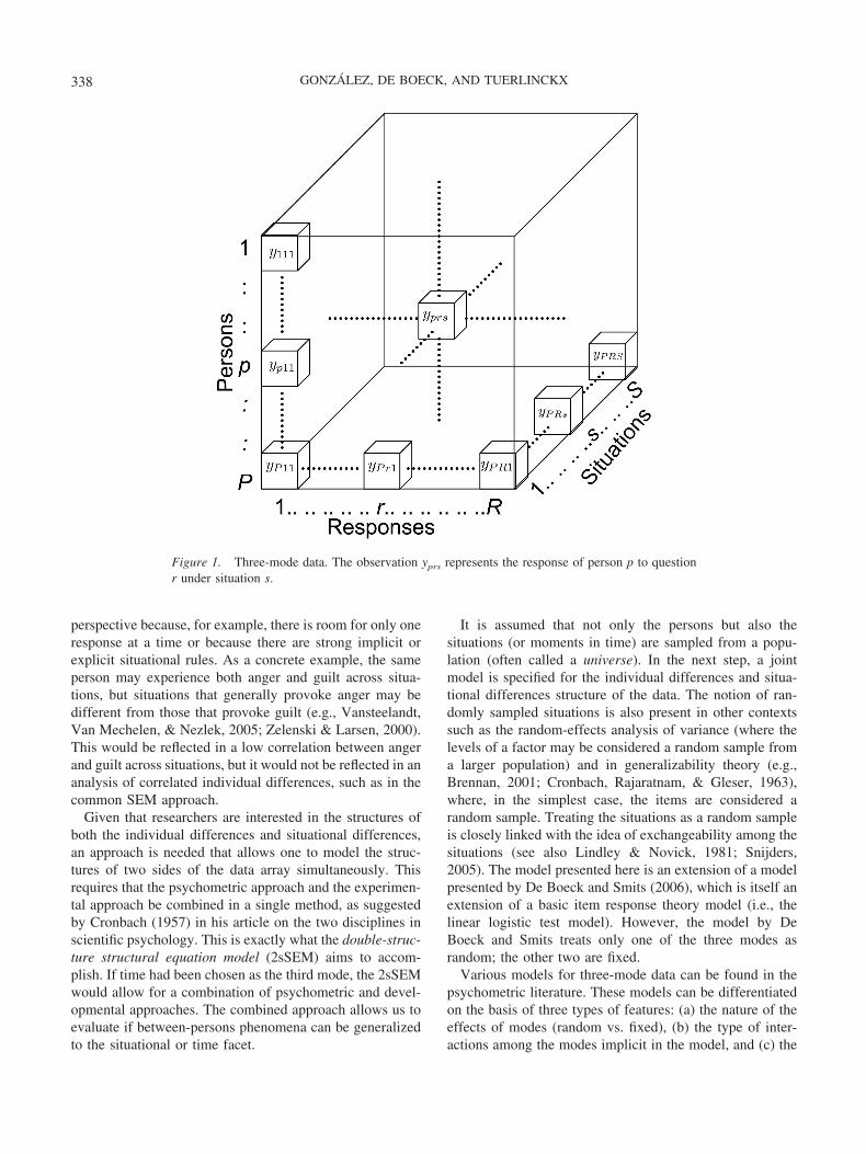
For the data that are analyzed in this article, a set of 679persons has been measured with respect to four emotionalresponses (frustration, tendency to act antagonistically, ir-ritation, and anger) in a set of 11 situations. Thus, thesituations are the third mode of the data. Figure 1 shows aschematic representation of the three-dimensional data arrayin which the observation yprs represents the response ofperson p (p � 1, . . ., P) to question r (r � 1, . . ., R) insituation s (s � 1, . . ., S).

In the context of the emotional response data set, it can behypothesized that the propensity of individuals to one re-sponse will be positively correlated to the propensity toother responses because of general underlying traits relatedto negative and positive affect. On the other hand, it ispossible that an emotional response may be less correlated,or even negatively correlated, to similar emotional re-sponses when one looks at the responses from a situational

Jorge Gonzalez, Paul De Boeck, and Francis Tuerlinckx, De-partment of Psychology, K. U. Leuven, Leuven, Belgium.

We have been partly supported by the Fund for ScientificResearch—Flanders (FWO) Grant No. G-0148-04 and by theK. U. Leuven Research Council Grant No. GOA/2005/04. Wewant to thank Betsy Feldman for her invaluable help with theediting of the article, in particular the English.

Correspondence concerning this article should be addressed toJorge Gonzalez, who is now at the Centro de Medicion MIDE UC,Pontificia Universidad Catolica de Chile, Vicuna Mackenna 4860,Macul, Santiago, Chile. E-mail: [email protected]

Psychological Methods2008, Vol. 13, No. 4, 337–353

Copyright 2008 by the American Psychological Association1082-989X/08/$12.00 DOI: 10.1037/a0013269

337

perspective because, for example, there is room for only oneresponse at a time or because there are strong implicit orexplicit situational rules. As a concrete example, the sameperson may experience both anger and guilt across situa-tions, but situations that generally provoke anger may bedifferent from those that provoke guilt (e.g., Vansteelandt,Van Mechelen, & Nezlek, 2005; Zelenski & Larsen, 2000).This would be reflected in a low correlation between angerand guilt across situations, but it would not be reflected in ananalysis of correlated individual differences, such as in thecommon SEM approach.

Given that researchers are interested in the structures ofboth the individual differences and situational differences,an approach is needed that allows one to model the struc-tures of two sides of the data array simultaneously. Thisrequires that the psychometric approach and the experimen-tal approach be combined in a single method, as suggestedby Cronbach (1957) in his article on the two disciplines inscientific psychology. This is exactly what the double-struc-ture structural equation model (2sSEM) aims to accom-plish. If time had been chosen as the third mode, the 2sSEMwould allow for a combination of psychometric and devel-opmental approaches. The combined approach allows us toevaluate if between-persons phenomena can be generalizedto the situational or time facet.

It is assumed that not only the persons but also thesituations (or moments in time) are sampled from a popu-lation (often called a universe). In the next step, a jointmodel is specified for the individual differences and situa-tional differences structure of the data. The notion of ran-domly sampled situations is also present in other contextssuch as the random-effects analysis of variance (where thelevels of a factor may be considered a random sample froma larger population) and in generalizability theory (e.g.,Brennan, 2001; Cronbach, Rajaratnam, & Gleser, 1963),where, in the simplest case, the items are considered arandom sample. Treating the situations as a random sampleis closely linked with the idea of exchangeability among thesituations (see also Lindley & Novick, 1981; Snijders,2005). The model presented here is an extension of a modelpresented by De Boeck and Smits (2006), which is itself anextension of a basic item response theory model (i.e., thelinear logistic test model). However, the model by DeBoeck and Smits treats only one of the three modes asrandom; the other two are fixed.

Various models for three-mode data can be found in thepsychometric literature. These models can be differentiatedon the basis of three types of features: (a) the nature of theeffects of modes (random vs. fixed), (b) the type of inter-actions among the modes implicit in the model, and (c) the

Figure 1. Three-mode data. The observation yprs represents the response of person p to questionr under situation s.

338 GONZALEZ, DE BOECK, AND TUERLINCKX

nature of dependence or independence among the responseswithin and across situations and within and across persons.These three features are discussed for all models underconsideration. For a short overview of these models, and inline with the application that is described later, it is assumedthat the three modes are persons, situations, and responses.Table 1 summarizes the differences among various possiblemodels. In Table 1 we use Fienberg’s (1980; see alsoAgresti, 2002) notation to express the interactions betweenvariables. The use of the term interaction may seem un-usual, but it makes sense when one considers that factorsand dimensions arise when elements of one mode (e.g.,persons) differ as a function of elements in a different mode(e.g., responses).

Two families of three-mode models can be discerned. Thefirst family originated with Tucker (1966), who proposed athree-mode principal-component model, now known as theTucker3 model. This type of model is the most general one,as far as interactions are concerned, because it includesthree-way interactions between persons, situations, and re-sponses. Each of the modes is analyzed in terms of itsprincipal components, and in principle, all combinations (allproducts) of the three kinds of components are included.The core matrix of these models determines the degree towhich each of the combinations plays a role. Because three-way interactions are considered, the lower order effects areimplied, unless the data array is first processed to eliminatemain effects (and possibly also pairwise interactions).

Depending on the specification of the core matrix, morerestricted versions of Tucker3 models can be obtained (seeKroonenberg, 1983, for an annotated bibliography). Forexample, in the CANDECOMP/PARAFAC model (Carroll& Chang, 1970; Harshman, 1970), each of the three modeshas the same number of factors. Within each mode, eachfactor is exclusively linked to one factor of each of the othertwo modes. As a result the core matrix takes a diagonalshape. In the original Tucker3 family, all parameters arefixed-effect parameters (see the column labeled Tucker3 (a)in Table 1). In a further development, the parameters refer-

ring to persons are considered to be random (e.g., Bentler &Lee, 1978, 1979; Bloxom, 1968; Lee & Fong, 1983; Oort,1999), as indicated in the column with heading Tucker3 (b)in Table 1. When all parameters are fixed, as is commonlythe case for the Tucker3 family, the issue of dependence andindependence is irrelevant, as indicated in Table 1. How-ever, if the persons are random, then the dependency struc-ture is the same as in the SEM for multitrait–multimethod(MTMM) data. This is explained next.

A second family of models is the set of SEMs forMTMM data (e.g., M. W. Browne, 1984; Eid, 2000; Eid,Lischetzke, & Nussbeck, 2006; Eid, Lischetzke, Nuss-beck, & Trierweiler, 2003). MTMM models are repre-sented in the column labeled SEM–MTMM in Table 1.Let us assume that the traits correspond to responses andthat the methods correspond to situations. In such mod-els, two types of factors (latent traits) occur: response(trait) factors and situation (method) factors. The effectsof trait and method factors on observed responses areadditive. Response factors reflect the interactions be-tween persons and responses and express individual dif-ferences based on those responses. Situation factors re-flect the interactions between persons and situations andexpress how the individual differences depend on thesituations. In other words, SEM–MTMM is focused onindividual differences, so it is not surprising that theperson mode is described in terms of random effects. Themodel utilizes a covariance structure across persons,which is decomposed into two kinds of covariation: thefirst resulting from individual differences related to re-sponses and the second from individual differences re-lated to situations. In SEM–MTMM, with observed vari-ables representing situation–response pairs, responses areassumed to be independent across individuals but corre-lated within individuals.

In contrast to the previous two models (Tucker3 andSEM–MTMM), the 2sSEM models the interactions of theresponses with persons and responses with situations (seeTable 1). In the former case, the latent factors refer to

Table 1Three Approaches for Modeling Three-Mode Data

Variable Tucker3 (a) Tucker3 (b) SEM–MTMM 2sSEM

Interactions �PSR� �PSR� �PS� �PR� �PR� �SR�Parameters

Persons fixed random random randomSituations fixed fixed fixed randomResponses fixed fixed fixed fixed

Dependence structureDependent irrelevant pairs (S, R) pairs (S, R) RIndependent irrelevant P P nonoverlapping pairs (P, S)

Note. Variables that interact are grouped together inside a set of brackets; variables that are independent of one another are placed in separate brackets.SEM–MTMM � structural equation model for multitrait–multimethod data; 2sSEM � double-structure structural equation model; P � persons; S �situations; R � responses.

339DOUBLE-STRUCTURE STRUCTURAL EQUATION MODELS

individual differences, and in the latter case they refer tosituational differences. Furthermore, the person mode andthe situation mode are both treated as random, so twodifferent covariance structures are considered: one overpersons and a second over situations. Finally, the observa-tions from different persons are not required to be indepen-dent, as is the case in the SEM–MTMM. Instead, person–situation pairs are assumed to be independent when theyhave neither the person nor the situation in common. SeeEquation 5 for the covariance structure of the 2sSEM.Because the SEM–MTMM is widely accepted and com-monly used for modeling Person � Situation � Responsedata and because the 2sSEM we are proposing is relativelynovel, we highlight the differences between the two models;see Table 1 for a summary.

1. The first distinction between the two models concernsindividual differences and situational differences. All latentvariables in the SEM–MTMM are individual-differencevariables because the persons are treated as random. In fact,two kinds of factors are named in SEM–MTMM: traitfactors and method factors. In the present context, situationsare equivalent to methods. Trait factors refer to interactionsbetween persons and responses. For example, anger andirritation are two of the responses in the example used inthis article. Without any interaction between persons andresponses, anger and irritation would have equal loadings.Generally speaking, if the individual trait levels do notdifferentially depend on the responses, then a single factoris required and all loadings will be equal. However, if theindividual differences do depend on the responses, multiplefactors with different loadings are likely. The presence ofmore than one factor indicates that there is interactionbetween persons and responses. In a similar way, situation(or method) factors refer to interactions between personsand situations (or methods). Hence, situational factors alsorefer to individual differences.

The 2sSEM also uses two types of latent variables. Thefirst type models individual differences, and the secondmodels situational differences. The individual differencefactors come about as a result of the interaction betweenpersons and responses (identical to the SEM–MTMM),whereas the situational difference factors are due to theinteraction between situations and responses; they capturedifferences that depend on the situation (but do not varyacross individuals). Suppose, for example, that a 2sSEMincludes anger and irritation factors. This implies that somesituations tend to generate anger, whereas other situationsare more likely to cause irritation. The 2sSEM and theSEM–MTMM situational factors are, therefore, fundamen-tally different.

2. The second difference concerns situations being treatedas random. In the 2sSEM, in contrast with the SEM–MTMM, the situation mode is also treated as random. Thisimplies that there is a universe of exchangeable situations

from which the researcher has randomly sampled a repre-sentative subset with the intent of generalizing across allsituations. For example, in this study we consider all pos-sible situations that may elicit anger or irritation and havesampled 11 exchangeable situations. In contrast, situationsor methods in SEM–MTMM are fixed and nonexchange-able. There is an inherent interest in discriminating amongindividual responses across a few specific and distinct sit-uations or methods. There could be reasons to be interestedin particular situations. For example, in a study investigat-ing situational differences in anger, one may concentrate onthe home environment and the work environment. Thesesituations are fixed and nonexchangeable, and the interest isin the covariance among the responses in these two majorsituations. Another implication of the assumption of randomsituation in 2sSEM is that the total number of situations isrelatively large compared to the number of fixed methods inSEM–MTMM. It is clear that they are to be treated as fixedand that there is not a large number of them.

3. The third distinction concerns independence assump-tions. Another important difference between SEM–MTMMand 2sSEM is the dependence structure they assume for theobservations. In the SEM–MTMM, the observations fromdifferent persons are independent. However, observationswithin an individual (i.e., from different situation–responsepairs) may be dependent. This is because situation–responsepairs, which constitute the variables or indicators in anSEM–MTMM, may correlate due to common (response orsituation) underlying latent variables. In the 2sSEM, obser-vations within an individual are expected to show depen-dence (this holds for responses both in the same situationand in different situations). However, observations fromdifferent persons within the same situation may also bedependent upon each other, because the situation may affectall persons in the same way. It is only for distinct person–situation pairs (with no common elements) that indepen-dence is assumed.

The remainder of the article is organized as follows: First,we introduce the data set we analyzed and formulate the basicresearch questions. Second, we introduce the 2sSEM using theconcepts underlying the regular SEM; Bayesian methods formodel estimation, model selection, and model checking arediscussed. To explain the model and to compare it with theSEM–MTMM, we use the normal linear version. Next, athree-mode data set (persons by situations by responses) aboutfour emotions is used to evaluate the model, and finally,conclusions and a discussion are presented.

Description of the Data

A central question in emotion research pertains to thedifferences between irritation and anger (e.g., Averill, 1982;Frijda, Kuipers, & ter Schure, 1989; Van Coillie & VanMechelen, 2006). Although the two emotions can be distin-


guished quite easily phenomenologically, it is still unclearin exactly what ways they differ. The componential theoryin emotion research forms a fruitful framework for studyingthis type of problem (Scherer, Schorr, & Johnstone, 2001).

The basic hypothesis underlying the theory is that emo-tions rely on two components, a feeling component and anaction-tendency component, and that the weight of eachmay differ depending on the emotion. Specifically, anger ishypothesized to be more action-oriented than irritation,whereas irritation is hypothesized to be more feeling-based.In addition, it is hypothesized that anger is primarily asso-ciated with an antagonistic action tendency and to a lesserdegree with frustration, whereas irritation is thought to beprimarily associated with the feeling of frustration.

The data in this article came from a sample of 679Dutch-speaking students in their last year of high school(Kuppens, Van Mechelen, Smits, De Boeck, & Ceulemans,2007). The students were presented with 11 situations,considered to be randomly drawn from a population ofsituations that might elicit negative emotional responses.They were asked to use a 4-point scale, ranging from 0 (notat all) to 3 (very strong), to indicate the degree to whichthey would experience frustration, a tendency to take an-tagonistic action, irritation, and anger. To simplify themodel construction, the original data were dichotomized byrecoding the values 0 and 1 as 0, and 2 and 3 as 1.Descriptions of the 11 situations are shown in Table 2.

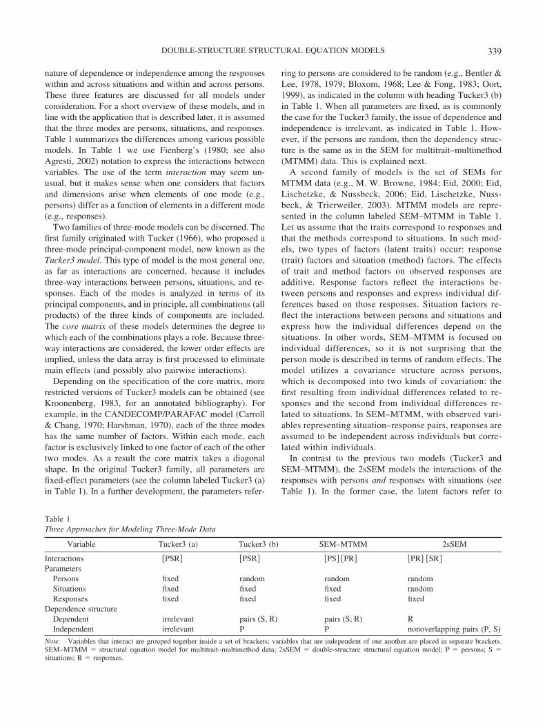
The histograms in Figure 2 show the proportions ofpositive answers (or endorsements) for each of the fourresponse types, aggregated over persons (Panel A) andsituations (Panel B). Panel A shows that, on average, ap-

proximately 70% of the 11 situations elicited endorsementsfor anger, frustration, and antagonistic action. Endorse-ments for irritation were more common, and there wasvariability in all four responses across the 11 situations.Panel B shows the proportions of endorsements for each ofthe four responses and for the 679 persons. The variabilityacross persons is visible in the plots. Many individualsshowed negative affect in all of the situations. The skeweddistribution on the manifest level might suggest a problem,but note that this is not necessarily a problem on the latentlevel. A normal distribution on the latent level may appearas a skewed distribution on the manifest level, depending onthe precise values of the situation and response parameters.These histograms show that, for both situations and persons,there is sufficient variability to investigate the covariancestructures.

After aggregating over either the situation or the personmode, the resulting two-way data can be fitted with astandard SEM; however, this approach has serious disad-vantages. After aggregating over situations, one can answeronly questions with respect to individual differences andcorrelations across individuals. Of course, it is possible tothen investigate the differences and the correlational struc-ture of the situations by aggregating over the person mode,but the net result of these actions is two unrelated models.For example, when aggregating over situations, it is possi-ble to investigate whether persons who tend to be angry alsotend to be irritated. Or, when aggregating over persons, onemight ask whether situations which tend to elicit anger alsotend to elicit irritation. The relationships between emotionalresponses in these two models may be similar, but this is notrequired.

The basic research questions addressed with these dataare as follows (see Figure 3 for a graphical representation):

1. What is the structure of the individual differences?If each emotional response (frustration, antagonis-tic action tendency, irritation, anger) is considereda separate latent variable over which individualscan differ, how are these latent variables related toone another? Is frustration the primary componentof irritation (i.e., vs. antagonistic action tendency),and is the tendency to act antagonistically theprimary component of anger (i.e., vs. frustration)?In terms of Figure 3, the hypothesis implied by thefirst research question is that a � c and that d � b.

2. What is the structure on the situation side? Is italso the case for situations that frustration is theprimary component of irritation and that antago-nistic action tendency is the primary component ofanger? The hypothesis is again that a � c and thatd � b in Figure 3, but now the figure refers tosituations rather than individuals.

Table 2Summary Descriptions of the Situations Used in the Study

Situation

You are blamed for someone else’s failures after a sports matchA fellow student loses your notes, causing you to fail the examA floppy disk holding an important school assignment is

destroyed by your computerYour sibling sneaks out when you both have to clean up the

houseBeing a work–study student yourself, an employee makes you

do all his choresA fellow student fails to return your notes the day before an

examAfter working hard on an assignment, your teacher says it’s still

not better than your previous workIt’s hard to study when the neighbors make a lot of noise and

it’s a hot dayA friend lets you down on an appointment to go out with his/

her friendYou’re at a party, and someone tells you that a friend outside

has smashed your bikeYou hear that a friend is spreading gossip about you


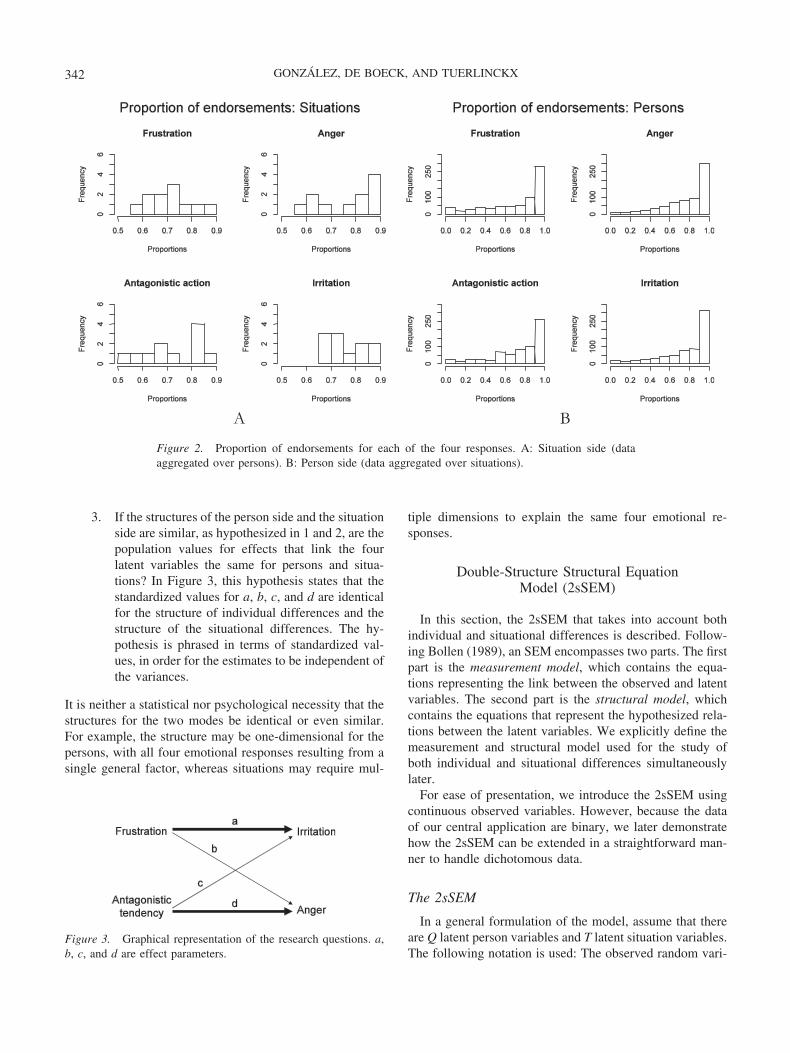
3. If the structures of the person side and the situationside are similar, as hypothesized in 1 and 2, are thepopulation values for effects that link the fourlatent variables the same for persons and situa-tions? In Figure 3, this hypothesis states that thestandardized values for a, b, c, and d are identicalfor the structure of individual differences and thestructure of the situational differences. The hy-pothesis is phrased in terms of standardized val-ues, in order for the estimates to be independent ofthe variances.

It is neither a statistical nor psychological necessity that thestructures for the two modes be identical or even similar.For example, the structure may be one-dimensional for thepersons, with all four emotional responses resulting from asingle general factor, whereas situations may require mul-

tiple dimensions to explain the same four emotional re-sponses.

Double-Structure Structural EquationModel (2sSEM)

In this section, the 2sSEM that takes into account bothindividual and situational differences is described. Follow-ing Bollen (1989), an SEM encompasses two parts. The firstpart is the measurement model, which contains the equa-tions representing the link between the observed and latentvariables. The second part is the structural model, whichcontains the equations that represent the hypothesized rela-tions between the latent variables. We explicitly define themeasurement and structural model used for the study ofboth individual and situational differences simultaneouslylater.

For ease of presentation, we introduce the 2sSEM usingcontinuous observed variables. However, because the dataof our central application are binary, we later demonstratehow the 2sSEM can be extended in a straightforward man-ner to handle dichotomous data.

The 2sSEM

In a general formulation of the model, assume that thereare Q latent person variables and T latent situation variables.The following notation is used: The observed random vari-

A B

Figure 2. Proportion of endorsements for each of the four responses. A: Situation side (dataaggregated over persons). B: Person side (data aggregated over situations).

Figure 3. Graphical representation of the research questions. a,b, c, and d are effect parameters.


able yprs represents the “magnitude” of person p’s responser in situation s. In the emotion data set, the index r may takeone of four values—1, 2, 3, or 4, which correspond tofrustration, antagonistic action tendency, irritation, and an-ger, respectively. The symbol �pq

PER refers to the score forperson p on the qth latent trait (q � 1, . . ., Q). Thesuperscript PER is somewhat superfluous because the sub-script p already indicates that the latent trait refers to theperson side and not the situation side. However, for thefactor loadings (�s, as in Equation 1) this difference will notbe as clear so we will retain the superscript notation. Like-wise, �st

SIT refers to the score for situation s on the tth latenttrait (t � 1, . . ., T). The effect of responses is represented by�r. From the description of the effects it is clear whether aneffect is fixed or random.

Measurement model. The measurement model weuse is

yprs � �q�1

Q

�rqPER�pq

PER � �t�1

T

�rtSIT�st

SIT � �r � εprs

� �rPER T

�pPER � �r

SIT T�s

SIT � �r � εprs, (1)

where �rqPER is the loading of response r on the qth (q �

1, . . ., Q) latent person variable, and �rtSIT is the loading of

response r on the tth (t � 1, . . ., T) latent situation variable.�r is the fixed general effect for response r, and εprs is arandom error term with mean zero. Both �pq

PER and �stSIT are

random variables, which are described when the structuralmodel is presented.

The measurement model in Equation 1 can also be writ-ten in matrix form. First, all responses pertaining to thesame person–situation combination are collected in the R �1 vector, yps. The row vectors of loadings (�r

PER Tand �r

SIT T)

are stacked in the loading matrices �PER and �SIT, respec-tively, and the �r parameters are gathered in one R � 1vector �. The model then becomes

yps � �PER �pPER � �SIT �s

SIT � � � �ps, (2)

or

�yp1s

�

yprs

�

ypRs

� � ��11

PER . . . �1QPER

� Ì �

�r1PER . . . �rQ

PER

� Ì �

�R1PER . . . �RQ

PER��

�p1PER

�

�pqPER

�

�pQPER

��

�11SIT . . . �1T

SIT

� Ì �

�r1SIT . . . �rT

SIT

� Ì �

�R1SIT . . . �RT

SIT��

�s1SIT

�

�stSIT

�

�sTSIT

� � ��1

�

�r

�

�R

� � �εp1s

�

εprs

�

εpRs

�. (3)

In a model for continuous and normally distributed data, onemay also assume that

�ps N(0,�),

where � is an R � R variance–covariance matrix of theerror terms. Usually � is taken to be diagonal. Note that wedefine a different distribution for the measurement errorterms in the case of binary data. In the most general case,there are as many latent variables as there are responses(Q � R and T � R). However, it is perfectly possible toformulate a model in which Q R and T R, and alsoQ � T. Given that, in the example, Q � R and T � R, notethat ypr1 to yprS are multiple indicators for �pr

PER, and simi-larly y1rs to yPrs are multiple indicators for �sr

SIT.(Double-structure) structural model. The two-fold

structural model can now be defined as follows:

�pPER � BPER �p

PER � �pPER

�sSIT � BSIT �s

SIT � �sSIT, (4)

where BPER and BSIT are Q � Q and T � T parametermatrices for regressions among the Q latent person vari-ables and among the T latent situation variables, respec-tively, and �p

PER and �sSIT are residual vectors. It is as-

sumed that both (I � BPER) and (I � BSIT) arenonsingular. A value of zero in a B matrix means thatthere is no effect of one latent variable on another. Inparticular, the diagonals of both BPER and BSIT alwayscontain only zeros, meaning that a variable is not ex-plained by itself.

Note that in Equation 4, a structure is imposed on boththe person latent variables and the situation latent vari-ables. Both �p

PER and �sSIT contain subvectors of latent

explanatory (independent or exogenous) and latent re-sponse (dependent or endogenous) variables. The resid-ual vectors �p

PER and �sSIT follow normal distributions

N(0,PER) and N(0,SIT), respectively, in which PER

and SIT contain covariances within and between the setsof explanatory and explained variables. In the models that areconsidered here, these covariances are assumed to be zerowhen an explained variable is involved but not when bothvariables are explanatory.

The standard graphical way of representing the SEM is apath diagram (e.g., Bollen, 1989). This graphical represen-tation of a system of simultaneous equations can be trans-ferred to the 2sSEM as well. Directional influence betweenthe variables is represented by single-headed arrows, andcurved two-headed arrows represent correlations. In theapplication that follows, we make use of the graphicalrepresentation to introduce several models (see Figure 4).The observed variables and error terms are omitted from thepath diagrams for clarity.

Having defined this model, it is possible to derive themodel-implied covariance matrices between the responsevectors yps and yp�s�:


Cov yps, yp�s�� PER I � BPER��1PER

� I � BPER�T�1�PER T� (5)

�SIT I � BSIT��1SIT I � BSIT�T�1�SIT T

��

if p � p� and s � s�

� �PER I � BPER��1PER I � BPER�T�1�PER T

if p � p� and s�s�

� �SIT I � BSIT��1SIT I � BSIT�T�1�SIT T

if p�p� and s � s�

� 0 if p�p� and s�s�.

As can be seen, in the linear 2sSEM, the model-impliedcovariance is nonzero for responses in two person–situationpairs that have at least one common element.

The model-implied covariance for an SEM–MTMMis a little different. The covariance is zero when p � p�, and itis � � � � when p � p�. The symbols , �, and � referto the trait covariance (covariance between individual differ-ences in the traits), the situation covariance (covariance be-tween individual differences associated with the situations),and the residual covariance matrices, respectively. All threerefer to individual differences.

Finally, note that the implied covariance structures hold onlyunder the normal linear model. In the remainder of the articlewe work with discrete (binary) data. For such data it is lesstrivial (but also less informative) to derive the implied covari-ance structure. However, under the 2sSEM it is still the casethat responses of different persons in the same situation andresponses of the same person in different situations are bothpermitted to be dependent (as well as responses by the sameindividual in the same situation).

The Model for Dichotomous Data

A latent threshold formulation is used to make the modelsuitable for analyzing binary data (details are given inAppendix A). Under this formulation, the measurementmodel in Equation 1 becomes a model for the conditionalprobability �prs � Pr yprs � 1��p

PER ,�sSIT� and is ex-

pressed as

�prs � F �rPER T

�pPER � �r

SIT T�s

SIT � �r�. (6)

We chose F to be F(x) � exp(x) / (1 � exp(x)), leading toa logistic model of the form

log� �prs

1 � �prs� � logit(�prs)

� �rPER T

�pPER � �r

SIT T�s

SIT � �r. (7)

The scale of the person and situation latent variables is thesame in terms of the effect on the logit scale, but the scaleis not standardized with respect to variance. Other selectionsof F are possible as well (e.g., if F equals the standardnormal cumulative distribution function, the result is a pro-bit model). The approach taken here to accommodate binaryvariables (and elaborated in Appendix A) can be extendedeasily to, for instance, ordinal data, by using the generalizedlinear model framework (GLM; McCullagh & Nelder,1989). For ordered-category data, one must make a choicebetween adjacent and cumulative logits. That is, either agiven category is compared with the one immediately belowit (adjacent logit), or the category of interest, together withall higher categories, is compared with all lower categories(cumulative logit). A simple way of doing this is to assumethat the distance between the category thresholds is thesame for all responses, so that the rating scale model (RSM;Andrich, 1978) can be used for either adjacent or cumula-tive logits. Skrondal and Rabe-Hesketh (2004) discussedhow GLMs may be incorporated into SEMs. Such an ap-proach greatly expands the area of application.

Statistical Inference

The 2sSEM includes random effects for two of the threemodes in the data; therefore, it is a crossed-random-effectsmodel (e.g., Janssen, Schepers, & Peres, 2004; Janssen,Tuerlinckx, Meulders, & De Boeck, 2000; Snijders &Bosker, 1999). When data are not normally distributed(such that the integral over the latent distribution has noanalytic solution), the estimation of model parameters is nottrivial (Tuerlinckx, Rijmen, Verbeke, & De Boeck, 2006).In this case, the likelihood contains an integral of a veryhigh dimension because, unlike a traditional random-effectsmodel, it cannot be factorized into separate contributions ofthe persons (because the responses of different persons arenot independent). The dimension of the integral over thelatent trait distributions is, at minimum, as high as the sumof the number of elements of the modes with random effects(in the central example in this article, that would mean atleast 690 dimensions), but in most cases, the dimensionalitywill be larger.

For such cases, the well-known Gauss–Hermite quadra-ture method becomes unfeasible, because of the high di-mensionality of the integrals in the likelihood function. AlsoLaplace approximations tend to break down because thedimensionality grows as a function of the sample size (e.g.,Shun, 1997; Shun & McCullagh, 1995). Possible alternativesolutions are Monte Carlo and Quasi-Monte Carlo methodsfor numerical integration (e.g., Gonzalez, Tuerlinckx, DeBoeck, & Cools, 2006) or Bayesian methodology, whichwas used in this article. In the following section, we outlinethe Bayesian method that was used to estimate the 2sSEM.Details of the estimation and software implementation are


given in Appendix B and the online supplemental material,respectively. Readers interested in more information aboutthe Bayesian approach for SEMs are referred to Lee (2007).

Bayesian Estimation

Bayesian inference is based on the posterior distributionof all parameters of interest, given the observed data. Let be the vector of parameters, as well as latent variables, andy the observed data. For the 2sSEM, contains all of theparameters in the matrices BPER, BSIT, �PER, �SIT, PER,SIT, and � and the latent residuals �p

PER ,�sSIT. If y | f(y

| ), then Bayes’s theorem leads to the following relation:

f( | y) � f(y | )f( ), (8)

which shows that the posterior density is proportional to thelikelihood function times the prior. A sample is obtained fromthe posterior distribution and the posterior mean, and posteriorstandard deviation and confidence intervals are used to sum-marize the distribution of each parameter of interest.

In order to obtain a sample from the posterior distribu-tion, different iterative methods belonging to the class ofMarkov Chain Monte Carlo (MCMC) techniques (e.g.,Gelman, Carlin, Stern, & Rubin, 2003) have been devel-oped. After the prior distributions are specified for all theparameters in the model, these algorithms generate aMarkov chain. Following an initial burn-in period (whichoften consists of several thousand iterations), the draws canbe used as a sample from the posterior distribution inEquation 8 on the condition that convergence is reached(which can be approximately checked using the R diagnos-tic; Gelman & Rubin, 1992).

WinBUGS (Spiegelhalter, Thomas, Best, & Lunn, 2003)is a software program for Bayesian analysis of statisticalmodels that uses MCMC techniques. After the user providesa likelihood and prior distribution, the program automati-cally draws a sample of all parameters from the posteriordistribution. Once convergence has been reached, parameterestimates can be obtained and inferences made.

All models in this article were fitted with WinBUGS,which was called from R (R Development Core Team,2006) by using the R2WinBUGS package (Sturtz, Ligges,& Gelman, 2005). Convergence was assessed using theCODA package (Plummer, Best, Cowles, & Vines, 2006),which implements standard convergence criteria (e.g.,Cowles & Carlin, 1996). The main R/WinBUGS code thatwas used is available as supplemental material online.

Bayesian Model Selection and Model Checking

When different models for data are fitted, the researcher isconfronted with a model selection issue: Which model fitsthe data best among the set of models under consideration?Because we are working in a Bayesian framework, we may

calculate Bayes factors (Kass & Raftery, 1995) and selectthe model with the largest posterior probability given thedata. However, it is quite computationally demanding tocompute Bayes factors, and therefore we considered othersolutions. The Akaike information criterion (AIC; Akaike,1974) and Bayesian information criterion (BIC; Schwarz,1978) provide alternative measures. However, these criteriaare derived in the frequentist framework and, therefore, areless applicable in our situation (although it is possible toestimate posterior AIC and BIC distributions on the basis ofthe draws from the posterior and compare those acrossdifferent models). Our preferred index for model selection isthe deviance information criterion (DIC; Spiegelhalter,Best, Carlin, & Van der Linde, 2002), which is easier tocompute than Bayes factors yet is a sufficiently theoreticallysound measure for model selection in a Bayesian frame-work. The DIC is calculated as a compromise betweenmodel fit and the number of effective parameters of themodel (in the same spirit as the more traditional modelselection methods such as AIC or BIC) and is defined as

DIC � D � � pD, (9)

where D � is the posterior mean of the deviance, used tomeasure model fit, and pD is an estimate of the effectivenumber of parameters. Lower values of the criterion indi-cate better fitting models (for more details, see Spiegelhalteret al., 2002).

After a model is selected, it is recommended that theresearcher evaluate the model’s global fit to the data. Forthis purpose we use samples from the posterior distributionvia posterior predictive checks (PPC; e.g., Gelman et al.,2003). The main idea behind PPC is that “if the model fits,then replicated data generated under the model should looksimilar to observed data” (Gelman et al., 2003, p. 165). Inaddition, a test quantity or discrepancy measure, T(y, ),which is calculated on the data and may depend on themodel parameters, may be used to measure the discrepancybetween specific features of the model and data. When thetest quantity T ·,·� does not depend on the model parameters,then it is called a test statistic, and it is denoted by T(y). Inthis case, lack of fit can be assessed by the tail-area prob-ability or p value of the test quantity. Note that the PPCprocedure allows one to choose any test quantity to check aparticular relevant aspect of the model. In practice, given adiscrepancy measure, T(y, ), the posterior predictive checkp value is calculated as follows:

1. Draw a vector (k) from the posterior distribution.

2. Simulate a replicated data set yrep k� from f(y | (k)).

3. Calculate T(y, (k)) and T yrep k� , k� �.

4. Repeat Steps 1 to 3 K times.


5. To obtain the posterior p value, count the propor-tion of replicated data sets yrep

k� for whichT yrep

k� , k� � � T y, k� �.

Note that when a test statistic T(y) is used, Step 3 does notrequire a model estimation at each iteration k but only thecalculation of T(y) and T yrep

k� � for each replicated data set.Details of the implementation of PPC in WinBUGS aregiven in the R/WinBUGS supplemental material online.

Another useful tool for assessing model fit is the graphicaldisplay. In the case of discrepancy measures, one can plotT yrep

k� , k� � and T(y, (k)) against each other. In the case of teststatistics one can compare T(y) with T yrep

1� �,�,T yrep k� � by local-

izing T(y) in the frequency distribution of T(yrep). In theApplication section of this article we use both a test quantity tocheck a particular aspect of our model and a global goodness-of-fit discrepancy measure.

Application

Model

Six models were fitted to the data.1 For convenience ofnotation, we represent frustration, antagonistic action ten-dency, irritation, and anger with indices 1, 2, 3, and 4,respectively.

The six models have the same measurement model but differstructurally. In general, the equations can be written as

logit �prs� � �prPER � �sr

SIT � �r Measurement model

(10)

and

�pPER � BPER �p

PER � �pPER Structural model

(11)

�sSIT � BSIT �s

SIT � �sSIT,

with p � 1, . . ., 679, r � 1, . . ., 4, and s � 1, . . ., 11. Giventhat the hypothesized latent variables are response specific(four latent variables, one for each emotion response), itseemed reasonable to adopt a strong hypothesis, stating thateach latent variable plays a role in only one kind of emotionresponse. Under this hypothesis, the factor-loading matricesin the measurement model do not contain any free param-eters, which is why �rq

PER and �stSIT from Equation 1 are no

longer needed in Equations 10 and 11. For every response,there is a single latent variable on the person side and aseparate one on the situation side so that in Equation 1�rq

PER � 1 when r � q, and 0 otherwise, and correspond-ingly, �rt

SIT � 1 when r � t, and 0 otherwise, with Q �T � 4.

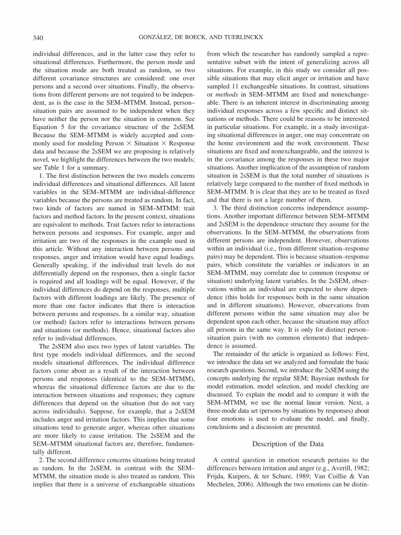
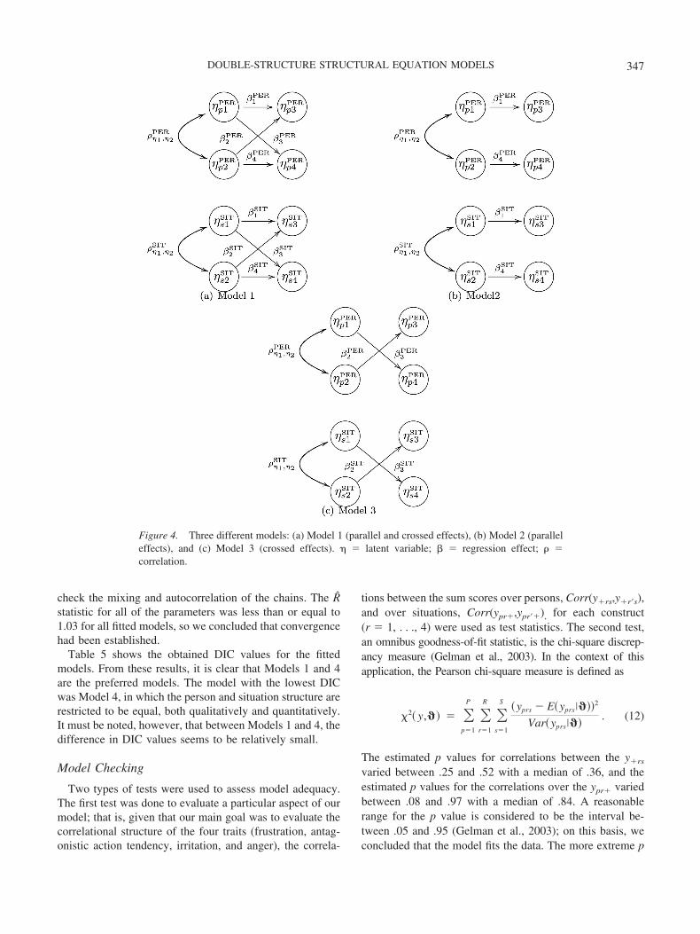
The six structural models are most clear when shown bygraphical representations. Figure 4 displays the path dia-

grams for three of the models (the remaining three modelsare derived from these). Model 1 (with parallel and crossedeffects) is the most general of the models; the latent re-sponse variables, irritation and anger, are each determinedby both of the latent explanatory variables, frustration andantagonistic tendency. Model 2 (with parallel effects) is theextreme form of the hypothesis mentioned earlier, statingthat irritation is based only on frustration and that angerresults solely from antagonistic action tendency. Model 3(with only crossed effects) is the opposite of Model 2, withirritation based exclusively on action tendency and angerresulting only from frustration. The corresponding parame-ter matrices BPER and BSIT of the three structural models areshown in Table 3. The three remaining models are con-structed by restricting the parameter matrices of the personand situation side to be equal (BPER � BSIT). These modelsare denoted as Models 4, 5, and 6, respectively.

Finally, as stated earlier, it is assumed that�p

PER � N 0,PER � and �sSIT � N 0,SIT �. Because we are

interested in a complete explanation of the third and fourthlatent variables, the covariances between �p3

PER, �p4PER, �s3

SIT, and�s4

SIT are all set to zero. In addition, the variances of �p3PER and

�p4PER, and of �s3

SIT and �s4SIT, are constrained to be equal

��3

PER � ��4

PER � ��PER, and ��3

SIT � ��4

SIT � ��SIT). A

model allowing different variances was also estimated, butthis did not result in a better fit. Table 4 shows the matrices for the fitted models. Note that because of the zerocorrelations among the residuals, the model is not a satu-rated SEM.

Estimation and Model Selection

A reparametrization of the model was used with hierar-chical centering (e.g., W. J. Browne, 2004; Gelfand, Sahu,& Carlin, 1995) in order to avoid poor mixing within chains.Five chains were run starting from different randomly se-lected initial values for the parameters of interest in each ofthe fitted models. This approach helps the researcher mon-itor convergence and choose an appropriate burn-in period.Each chain was run with 5,000 iterations, and the first halfof each chain was discarded as a burn-in stage. For theinferences and model checking we accepted every 5th drawof the remaining 2,500 draws of each of the five chains.Using nonconsecutive draws helps reduce autocorrelationand avoid dependence between subsequent draws. Thus, theresults that are reported are based on a final sample of 2,500iterations.

The R (Gelman & Rubin, 1992) was used to assessconvergence. Values of R near 1.0 (say, below 1.1) areconsidered acceptable (Gelman et al., 2003, pp. 296–297).Also, graphical tools implemented in CODA were used to

1 The data and the R-WinBUGS code used in this section areavailable in the supplemental online materials.


check the mixing and autocorrelation of the chains. The Rstatistic for all of the parameters was less than or equal to1.03 for all fitted models, so we concluded that convergencehad been established.

Table 5 shows the obtained DIC values for the fittedmodels. From these results, it is clear that Models 1 and 4are the preferred models. The model with the lowest DICwas Model 4, in which the person and situation structure arerestricted to be equal, both qualitatively and quantitatively.It must be noted, however, that between Models 1 and 4, thedifference in DIC values seems to be relatively small.

Model Checking

Two types of tests were used to assess model adequacy.The first test was done to evaluate a particular aspect of ourmodel; that is, given that our main goal was to evaluate thecorrelational structure of the four traits (frustration, antag-onistic action tendency, irritation, and anger), the correla-

tions between the sum scores over persons, Corr(y�rs,y�r�s),and over situations, Corr(ypr�,ypr��), for each construct(r � 1, . . ., 4) were used as test statistics. The second test,an omnibus goodness-of-fit statistic, is the chi-square discrep-ancy measure (Gelman et al., 2003). In the context of thisapplication, the Pearson chi-square measure is defined as

�2 y, � � �p�1

P �r�1

R �s�1

S yprs � E yprs� ��2

Var yprs� �. (12)

The estimated p values for correlations between the y�rs

varied between .25 and .52 with a median of .36, and theestimated p values for the correlations over the ypr� variedbetween .08 and .97 with a median of .84. A reasonablerange for the p value is considered to be the interval be-tween .05 and .95 (Gelman et al., 2003); on this basis, weconcluded that the model fits the data. The more extreme p

Figure 4. Three different models: (a) Model 1 (parallel and crossed effects), (b) Model 2 (paralleleffects), and (c) Model 3 (crossed effects). � � latent variable; � � regression effect; � �correlation.


values obtained when using correlations for ypr� are aconsequence of the smaller number of situations considered.

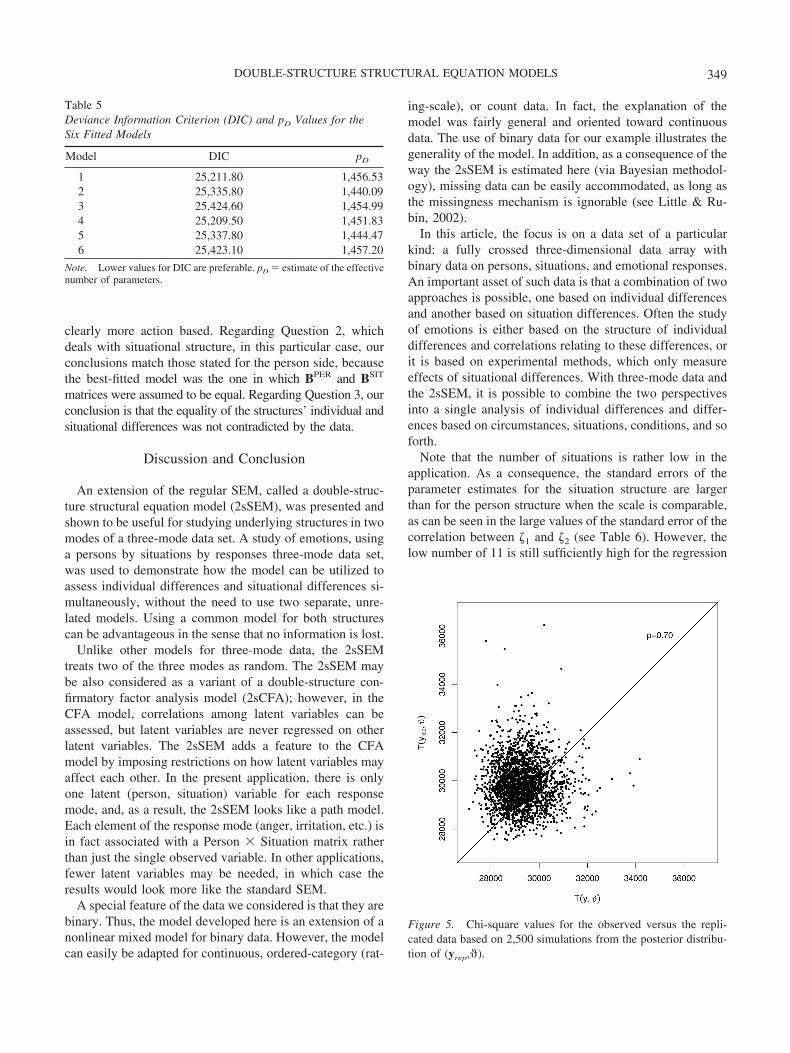
Figure 5 shows a scatter plot of the chi-square test quan-tity evaluated for observed and replicated data. The poste-rior p value (.70) reported in the figure is calculated as theproportion of points above the diagonal line (i.e., the pro-portion of replicated values that are larger than the observedones). From Figure 5 it can be concluded that the model fitsthe data reasonably well in a global way as well.

Results

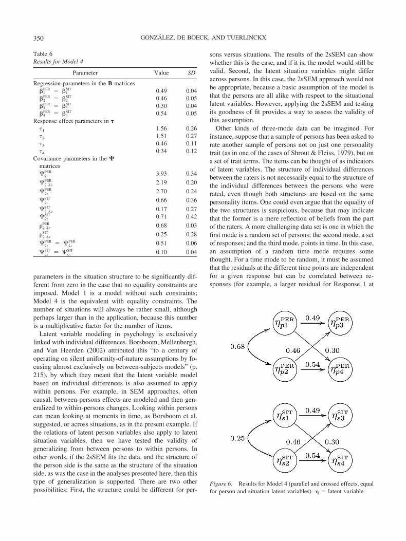
Table 6 shows the posterior means and standard devia-tions of the parameters in Model 4, and Figure 6 containsthe graphical representation of the structural part of Model4, including the parameter estimates. In latent person andlatent situation structures, frustration and the antagonisticaction tendency affected both irritation and anger. As ex-pected, the feeling of frustration was more important forirritation than the antagonistic tendency, whereas the oppo-site was true in the case of anger. In the case of irritation, thedifference was very small (.49 vs. .46), but for anger it wasmuch larger (.54 vs. .30). The correlation between theexplanatory latent person variables was moderately highand positive (.68), whereas the correlation between theexplanatory latent situation variables was much lower butstill positive (.25). The posterior standard deviation for

correlation on the situation side was larger than the one onthe person side due to the smaller sample of situations. Thedifference in correlations can be explained by the differencein variance; the situations seem much more homogeneousthan the persons. This difference in correlations is also inagreement with earlier findings (Vansteelandt et al., 2005;Zelenski & Larsen, 2000).

The � parameters must be interpreted as indicating the prob-ability of showing each of the four responses when all latentvariables are set to zero (on the logistic scale). For instance, foran average person in an average situation, the probabilities ofendorsing responses 1 and 2 (see Table 6) equal

�p1s �exp 1.56�

1 � exp 1.56�� 0.83, and

�p2s �exp 1.51�

1 � exp 1.51�� 0.82, (13)

respectively. The two responses are approximately equallylikely.

The primary hypotheses of the study were confirmed bythe analyses. The questions mentioned in the second sectionof this article can now be answered in the following way:Regarding Question 1, on the basis of the BPER matrix, weconclude that irritation seems to be slightly more feelingbased but the difference is negligible, whereas anger is

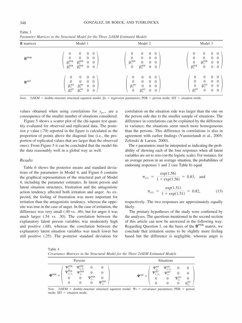
Table 3Parameter Matrices in the Structural Model for the Three 2sSEM Estimated Models

B matrices Model 1 Model 2 Model 3

BPER �0 0 0 00 0 0 0

�1PER �2

PER 0 0�3

PER �4PER 0 0

� �0 0 0 00 0 0 0

�1PER 0 0 00 �4

PER 0 0� �

0 0 0 00 0 0 00 �2

PER 0 0�3

PER 0 0 0�

BSIT �0 0 0 00 0 0 0

�1SIT �2

SIT 0 0�3

SIT �4SIT 0 0

� �0 0 0 00 0 0 0

�1SIT 0 0 00 �4

SIT 0 0� �

0 0 0 00 0 0 00 �2

SIT 0 0�3

SIT 0 0 0�

Note. 2sSEM � double-structure structural equation model. �s � regression parameters; PER � person mode; SIT � situation mode.

Table 4Covariance Matrices in the Structural Model for the Three 2sSEM Estimated Models

Persons Situations

PER � ��1

PER ��1,�2

PER 0 0��

2,�

1

PER��2

PER 0 0

0 0 ��3

PER 00 0 0 ��4

PER� SIT � �

��1

SIT ��1,�2

SIT 0 0��

2,�

1

SIT��1

SIT 0 0

0 0 ��3

SIT 00 0 0 ��4

SIT�

Note. 2sSEM � double-structure structural equation model. �s � covariance parameters; PER � personmode; SIT � situation mode.


clearly more action based. Regarding Question 2, whichdeals with situational structure, in this particular case, ourconclusions match those stated for the person side, becausethe best-fitted model was the one in which BPER and BSIT

matrices were assumed to be equal. Regarding Question 3, ourconclusion is that the equality of the structures’ individual andsituational differences was not contradicted by the data.

Discussion and Conclusion

An extension of the regular SEM, called a double-struc-ture structural equation model (2sSEM), was presented andshown to be useful for studying underlying structures in twomodes of a three-mode data set. A study of emotions, usinga persons by situations by responses three-mode data set,was used to demonstrate how the model can be utilized toassess individual differences and situational differences si-multaneously, without the need to use two separate, unre-lated models. Using a common model for both structurescan be advantageous in the sense that no information is lost.

Unlike other models for three-mode data, the 2sSEMtreats two of the three modes as random. The 2sSEM maybe also considered as a variant of a double-structure con-firmatory factor analysis model (2sCFA); however, in theCFA model, correlations among latent variables can beassessed, but latent variables are never regressed on otherlatent variables. The 2sSEM adds a feature to the CFAmodel by imposing restrictions on how latent variables mayaffect each other. In the present application, there is onlyone latent (person, situation) variable for each responsemode, and, as a result, the 2sSEM looks like a path model.Each element of the response mode (anger, irritation, etc.) isin fact associated with a Person � Situation matrix ratherthan just the single observed variable. In other applications,fewer latent variables may be needed, in which case theresults would look more like the standard SEM.

A special feature of the data we considered is that they arebinary. Thus, the model developed here is an extension of anonlinear mixed model for binary data. However, the modelcan easily be adapted for continuous, ordered-category (rat-

ing-scale), or count data. In fact, the explanation of themodel was fairly general and oriented toward continuousdata. The use of binary data for our example illustrates thegenerality of the model. In addition, as a consequence of theway the 2sSEM is estimated here (via Bayesian methodol-ogy), missing data can be easily accommodated, as long asthe missingness mechanism is ignorable (see Little & Ru-bin, 2002).

In this article, the focus is on a data set of a particularkind: a fully crossed three-dimensional data array withbinary data on persons, situations, and emotional responses.An important asset of such data is that a combination of twoapproaches is possible, one based on individual differencesand another based on situation differences. Often the studyof emotions is either based on the structure of individualdifferences and correlations relating to these differences, orit is based on experimental methods, which only measureeffects of situational differences. With three-mode data andthe 2sSEM, it is possible to combine the two perspectivesinto a single analysis of individual differences and differ-ences based on circumstances, situations, conditions, and soforth.

Note that the number of situations is rather low in theapplication. As a consequence, the standard errors of theparameter estimates for the situation structure are largerthan for the person structure when the scale is comparable,as can be seen in the large values of the standard error of thecorrelation between �1 and �2 (see Table 6). However, thelow number of 11 is still sufficiently high for the regression

Figure 5. Chi-square values for the observed versus the repli-cated data based on 2,500 simulations from the posterior distribu-tion of (yrep,�).

Table 5Deviance Information Criterion (DIC) and pD Values for theSix Fitted Models

Model DIC pD

1 25,211.80 1,456.532 25,335.80 1,440.093 25,424.60 1,454.994 25,209.50 1,451.835 25,337.80 1,444.476 25,423.10 1,457.20

Note. Lower values for DIC are preferable. pD � estimate of the effectivenumber of parameters.


parameters in the situation structure to be significantly dif-ferent from zero in the case that no equality constraints areimposed. Model 1 is a model without such constraints;Model 4 is the equivalent with equality constraints. Thenumber of situations will always be rather small, althoughperhaps larger than in the application, because this numberis a multiplicative factor for the number of items.

Latent variable modeling in psychology is exclusivelylinked with individual differences. Borsboom, Mellenbergh,and Van Heerden (2002) attributed this “to a century ofoperating on silent uniformity-of-nature assumptions by fo-cusing almost exclusively on between-subjects models” (p.215), by which they meant that the latent variable modelbased on individual differences is also assumed to applywithin persons. For example, in SEM approaches, oftencausal, between-persons effects are modeled and then gen-eralized to within-persons changes. Looking within personscan mean looking at moments in time, as Borsboom et al.suggested, or across situations, as in the present example. Ifthe relations of latent person variables also apply to latentsituation variables, then we have tested the validity ofgeneralizing from between persons to within persons. Inother words, if the 2sSEM fits the data, and the structure ofthe person side is the same as the structure of the situationside, as was the case in the analyses presented here, then thistype of generalization is supported. There are two otherpossibilities: First, the structure could be different for per-

sons versus situations. The results of the 2sSEM can showwhether this is the case, and if it is, the model would still bevalid. Second, the latent situation variables might differacross persons. In this case, the 2sSEM approach would notbe appropriate, because a basic assumption of the model isthat the persons are all alike with respect to the situationallatent variables. However, applying the 2sSEM and testingits goodness of fit provides a way to assess the validity ofthis assumption.

Other kinds of three-mode data can be imagined. Forinstance, suppose that a sample of persons has been asked torate another sample of persons not on just one personalitytrait (as in one of the cases of Shrout & Fleiss, 1979), but ona set of trait terms. The items can be thought of as indicatorsof latent variables. The structure of individual differencesbetween the raters is not necessarily equal to the structure ofthe individual differences between the persons who wererated, even though both structures are based on the samepersonality items. One could even argue that the equality ofthe two structures is suspicious, because that may indicatethat the former is a mere reflection of beliefs from the partof the raters. A more challenging data set is one in which thefirst mode is a random set of persons; the second mode, a setof responses; and the third mode, points in time. In this case,an assumption of a random time mode requires somethought. For a time mode to be random, it must be assumedthat the residuals at the different time points are independentfor a given response but can be correlated between re-sponses (for example, a larger residual for Response 1 at

Figure 6. Results for Model 4 (parallel and crossed effects, equalfor person and situation latent variables). � � latent variable.

Table 6Results for Model 4

Parameter Value SD

Regression parameters in the B matrices�1

PER � �1SIT 0.49 0.04

�2PER � �2

SIT 0.46 0.05�3

PER � �3SIT 0.30 0.04

�4PER � �4

SIT 0.54 0.05Response effect parameters in �

�1 1.56 0.26�2 1.51 0.27�3 0.46 0.11�4 0.34 0.12

Covariance parameters in the matrices��1

PER 3.93 0.34

��1,�2

PER 2.19 0.20

��2

PER 2.70 0.24

��1

SIT 0.66 0.36

��1,�2

SIT 0.17 0.27��2

SIT 0.71 0.42

��1,�2

PER 0.68 0.03

��1,�2

SIT 0.25 0.28

��3

PER � ��4

PER 0.51 0.06

��3

SIT � ��4

SIT 0.10 0.04


time point t is more likely to co-occur with a larger residualfor Response 2 at the same time point). Additionally, onemay assume more refined structural relations between thesewithin-time-point residuals.

The 2sSEM is a useful model for combining and com-paring the structures of two modes in terms of a third modewithin a data set concerning, for example, emotions, as inthe application shown here, or personality, as in the appli-cation about which we speculated. However, a 2sSEM is notappropriate for all three-mode data. For example, only twotypes of interactions may be accounted for, as shown inTable 1. In our application, these were persons by responsesand situations by responses. The roles of the three kinds ofentities may be changed, but if these two pairwise interac-tions are modeled, then it is not possible to include the thirdinteraction—that of persons and situations. In other words,for this model to be useful, the introduction of two types oflatent variables, one for each of two of the three modes,must be meaningful.

References

Agresti, A. (2002). Categorical data analysis (2nd ed.). Hoboken,NJ: Wiley.

Akaike, M. (1974). A new look at the statistical model identifica-tion. IEEE Transactions on Automatic Control, 19, 716–723.

Andrich, D. (1978). A rating scale formulation for ordered re-sponse categories. Psychometrika, 43, 561–573.

Averill, J. (1982). Anger and aggression: An essay on emotion.New York: Springer.

Bentler, P., & Lee, S.-Y. (1978). Statistical aspects of a three-modefactor analysis model. Psychometrika, 43, 343–352.

Bentler, P., & Lee, S.-Y. (1979). A statistical development ofthree-mode factor analysis. British Journal of Mathematical andStatistical Psychology, 32, 87–104.

Bloxom, B. (1968). A note on invariance in three-mode factoranalysis. Psychometrika, 33, 347–350.

Bollen, K. (1989). Structural equations with latent variables. NewYork: Wiley.

Borsboom, D., Mellenbergh, G., & Van Heerden, J. (2002). Thetheoretical status of latent variables. Psychological Review, 110,203–219.

Brennan, R. L. (2001). Generalizability theory. New York: Spring-er-Verlag.

Browne, M. W. (1984). The decomposition of multitrait–multi-method matrices. British Journal of Mathematical and Statisti-cal Psychology, 37, 1–21.

Browne, W. J. (2004). An illustration of the use of reparameterisationmethods for improving MCMC efficiency in crossed random ef-fects models. Multilevel Modelling Newsletter, 16, 13–25.

Carroll, J., & Chang, J. (1970). Analysis of individual differencesin multidimensional scaling via an N-way generalization ofEckart–Young decomposition. Psychometrika, 35, 283–319.

Cattell, R. (1946). Description and measurement of personality.New York: World Book Cie.

Cattell, R. (1952). Factor analysis: An introduction and manualfor the psychologist and social scientist. New York: Harper.

Cowles, M., & Carlin, B. (1996). Markov Chain Monte Carloconvergence diagnostics: A comparative study. Journal of theAmerican Statistical Association, 91, 883–904.

Cronbach, L. (1957). The two disciplines of scientific psychology.American Psychologist, 12, 671–684.

Cronbach, L., Rajaratnam, N., & Gleser, G. (1963). Theory of gen-eralizability: A liberalization of reliability theory. British Journal ofMathematical and Statistical Psychology, 16, l37–163.

De Boeck, P., & Smits, D. (2006). A double-structure structuralequation model for the study of emotions and their components. InQ. Jing et al. (Eds.), Progress in psychological science around theworld: Vol. 1. Neural, cognitive and developmental issues (pp.349–365). Hove, United Kingdom: Psychology Press.

Eid, M. (2000). A multitrait–multimethod model with minimalassumptions. Psychometrika, 65, 241–261.

Eid, M., Lischetzke, T., & Nussbeck, F. (2006). Structural equa-tion models for multitrait–multimethod data. In M. Eid & E.Diener (Eds.), Handbook of psychological measurement: A mul-timethod perspective (pp. 283–299). Washington, DC: Ameri-can Psychological Association.

Eid, M., Lischetzke, T., Nussbeck, F., & Trierweiler, L. (2003).Separating trait effects from trait-specific method effects inmultitrait–multimethod analysis: A multiple indicatorCTC(M-1) model. Psychological Methods, 8, 38–60.

Fienberg, S. (1980). The analysis of cross-classified, categoricaldata (2nd ed.). Cambridge, MA: MIT Press.

Frijda, N., Kuipers, P., & ter Schure, E. (1989). Relations amongemotion, appraisal, and emotional action readiness. Journal ofPersonality and Social Psychology, 65, 942–958.

Gelfand, A., Sahu, S., & Carlin, B. (1995). Efficient parameterizationsfor normal linear mixed models. Biometrika, 82, 479–488.

Gelman, A., Carlin, J., Stern, H., & Rubin, D. (2003). Bayesiandata analysis (2nd ed.). New York: Chapman and Hall.

Gelman, A., & Rubin, D. (1992). Inference from iterative simula-tion using multiple sequences (with discussion). Statistical Sci-ence, 7, 457–511.

Gonzalez, J., Tuerlinckx, F., De Boeck, P., & Cools, R. (2006).Numerical integration in logistic-normal models. Computa-tional Statistics and Data Analysis, 51, 1535–1548.

Harshman, R. (1970). Foundations of the PARAFAC procedure:Models and conditions for an “explanatory” multi-mode factoranalysis. UCLA Working Papers in Phonetics, 16, 1–84.

Janssen, R., Schepers, J., & Peres, D. (2004). Models with itemand item group predictors. In P. De Boeck & M. Wilson (Eds.),Explanatory item response models: A generalized linear andnonlinear approach (pp. 189–212). New York: Springer.

Janssen, R., Tuerlinckx, F., Meulders, M., & De Boeck, P. (2000).A hierarchical IRT model for criterion-referenced measurement.Journal of Educational and Behavioral Statistics, 25, 285–306.


Kass, R., & Raftery, A. (1995). Bayes factors. Journal of theAmerican Statistical Association, 90, 773–796.

Kroonenberg, P. (1983). Annotated bibliography of three-modefactor analysis. British Journal of Mathematical and StatisticalPsychology, 36, 81–113.

Kroonenberg, P. (2005). Three-mode component and scaling meth-ods. In B. Everitt & D. Howell (Eds.), Encyclopedia of statistics inbehavioral science (Vol. 4, pp. 2032–2044). New York: Wiley.

Kuppens, P., Van Mechelen, I., Smits, D., De Boeck, P., & Ceule-mans, E. (2007). Individual differences in patterns of appraisal andanger experience. Cognition & Emotion, 21, 689–713.

Lee, S.-Y. (2007). Structural equation modeling: A Bayesian ap-proach. Chichester, United Kingdom: Wiley.

Lee, S.-Y., & Fong, W.-K. (1983). A scale invariant model forthree-mode factor analysis. British Journal of Mathematical andStatistical Psychology, 36, 217–223.

Lindley, D. V., & Novick, M. R. (1981). The role of exchange-ability in inference. Annals of Statistics, 9, 45–58.

Little, R., & Rubin, D. (2002). Statistical analysis with missingdata (2nd ed.). Chichester, United Kingdom: Wiley.

McCullagh, P., & Nelder, J. (1989). Generalized linear models.New York: Chapman & Hall.

Oort, F. (1999). Stochastic three-mode models for mean and co-variance structures. British Journal of Mathematical and Statis-tical Psychology, 52, 243–272.

Plummer, M., Best, N., Cowles, K., & Vines, K. (2006, March).CODA: Convergence diagnosis and output analysis for MCMC.R News, 6(1), 7–11. Available from http://cran.r-project.org/doc/Rnews/Rnews_2006–1.pdf

R Development Core Team. (2006). R: A language and environ-ment for statistical computing [Computer software manual].Available from http://www.R-project.org

Scherer, K., Schorr, A., & Johnstone, T. (2001). Appraisal pro-cesses in emotion: Theory, methods, research. New York: Ox-ford University Press.

Schwarz, G. (1978). Estimating the dimension of a model. TheAnnals of Statistics, 6, 461–464.

Shrout, P. E., & Fleiss, J. L. (1979). Intraclass correlations: Uses inassessing rater reliability. Psychological Bulletin, 2, 420–428.

Shun, Z. (1997). Another look at the salamander mating data: Amodified Laplace approximation approach. Journal of the Amer-ican Statistical Association, 92, 341–349.

Shun, Z., & McCullagh, P. (1995). Laplace approximation of highdimensional integrals. Journal of the Royal Statistical Society,57(B), 749–760.

Skrondal, A., & Rabe-Hesketh, S. (2004). Generalized latent vari-able modeling: Multilevel, longitudinal, and structural equa-tions models. Boca Raton, FL: Chapman and Hall/CRC.

Snijders, T. (2005). Fixed and random effects. In B. S. Everitt & D. C.Howell (Eds.), Encyclopedia of statistics in behavioral science(Vol. 2, pp. 664–665). Chichester, United Kingdom: Wiley.

Snijders, T., & Bosker, R. (1999). Multilevel analysis: An introduc-tion to basic and advanced multilevel modeling. London: Sage.

Spiegelhalter, D., Best, N., Carlin, B., & Van der Linde, A. (2002).Bayesian measures of model complexity and fit. Journal of theRoyal Statistical Society, 64(B), 583–639.

Spiegelhalter, D., Thomas, A., Best, N., & Lunn, D. (2003).WinBUGS Version 1.4 user manual [Computer software man-ual]. Retrieved from http://www.mrc-bsu.cam.ac.uk/bugs/winbugs/manual14.pdf

Sturtz, S., Ligges, U., & Gelman, A. (2005). R2WinBUGS: Apackage for running WinBUGS from R. Journal of StatisticalSoftware, 12(3), 1–16. Retrieved from http://www.jstatsoft.org/v12/i03/paper

Tucker, L. (1966). Some mathematical notes on three-mode factoranalysis. Psychometrika, 31, 279–311.

Tuerlinckx, F., Rijmen, F., Verbeke, G., & De Boeck, P. (2006).Statistical inference in generalized linear mixed models: A review.British Journal of Mathematical and Statistical Psychology, 59,225–255.

Van Coillie, H., & Van Mechelen, I. (2006). A taxonomy of anger-relatedbehaviors in young adults. Motivation and Emotion, 30, 57–74.

Vansteelandt, K., Van Mechelen, I., & Nezlek, J. (2005). Theco-occurrence of emotions in daily life: A multilevel approach.Journal of Research in Personality, 39, 325–335.

Zelenski, J., & Larsen, R. (2000). The distribution of basic emotionsin everyday life: A state and trait perspective from experiencesampling data. Journal of Research in Personality, 34, 178–197.


Appendix A

Latent Threshold Formulation of the Model for Analyzing Binary Data

The measurement part of the 2sSEM can handle bothcontinuous and binary observed variables. To illustrate this,we relate the observed yprs variables to a continuous latentresponse variable yprs

� .Consider the following linear regression model for con-

tinuous response variable yprs� :

yprs� � �prs � εprs, (14)

where �prs � �rPER T

�pPER � �r

SIT T�s

SIT � �r is the bilin-ear predictor used for the 2sSEM, and εprs is an error termof mean zero. This model can alternatively be defined as

E yprs� ��prs� � �prs. (15)

In the case of continuous responses, the latent responseequals the observed response: yprs � yprs

� .In the case of binary responses, the response variable is

defined by the following threshold model:

yprs � � 1, if yprs� � 0

0, otherwise. (16)

It follows that

E yprs��prs� � Pr yprs � 1��prs� � �prs

� Pr yprs� � 0��prs�

� Pr �prs � εprs � 0�

� Pr εprs � � �prs�

� F �prs�, (17)

where the last equality is due to the symmetry of the distribu-tion function F of εprs. Typically, F is chosen to be either thecumulative standard normal or logistic distribution. In thisarticle, the logistic distribution was assumed such that

F�1 �prs� � log� �prs

1 � �prs� � logit �prs� � �prs

� �rPER T

�pPER � �r

SIT T�s

SIT � �r, (18)

where F�1 x� � log� x

1 � x� � logit x� is the link function.

Appendix B

Derivation of the Posterior Distribution

Assuming conditional independence, the likelihood func-tion for binary data is written as

f(y� ) � ��p�1

P �r�1

R �s�1

S

F(�prs)yprs�1�F(�prs)�

1�yprs�, (19)

where F(vprs) � �prs (see Appendix A).In order to have a sample of we need to specify prior

distributions for all the involved parameters. For the param-eters in BPER, BSIT, and �, normal diffuse priors with meanzero and variance 104 were chosen. For the upper left blockof the covariance matrices PER and SIT (i.e., the vari-ances and covariance of the latent explanatory variables),inverse-Wishart prior distributions with scale matrix 103Iand 2 degrees of freedom were chosen. For the variances ofthe latent residuals (i.e., the diagonal elements of the lowerright block of the matrices), inverse-gamma distributionswith both shape and scale parameters equal to 104 werechosen. Finally, the distribution for the latent person and

situation residuals are given by the model assumptions andare multivariate normal distributions with zero vector meanand covariance matrices PER and SIT, respectively.

Using the relation in Equation 8, the posterior distribution isthen given by the product of the likelihood in Equation 19 and

f � � �p�1

P

N �pPER ;0,PER ��

s�1

S

N �sSIT;0,SIT �

� p(BPER )p(BSIT )p �� p PER �p SIT �, (20)

where N(Z;�,�) means that the random vector Z is distributedas a multivariate normal distribution with vector mean � andcovariance matrix �. Note that independence of the priors isassumed.

Received December 5, 2006Revision received July 7, 2008

Accepted July 7, 2008 �


A double-structure structural equation model for three-mode data

Documents

Transcript of A double-structure structural equation model for three-mode data