A distributed multi‑agent system approach for solving ...

This document is downloaded from DR‑NTU (https://dr.ntu.edu.sg)Nanyang Technological University, Singapore.

A distributed multi‑agent system approach forsolving constrained optimization problems usingprobability collectives

Anand Jayant Kulkarni

2012

Anand Jayant Kulkarni. (2012). A distributed multi‑agent system approach for solvingconstrained optimization problems using probability collectives. Doctoral thesis, NanyangTechnological University, Singapore.

https://hdl.handle.net/10356/48033

https://doi.org/10.32657/10356/48033

Downloaded on 10 Feb 2022 10:30:16 SGT

A DISTRIBUTED MULTI-AGENT SYSTEM

APPROACH FOR SOLVING CONSTRAINED

OPTIMIZATION PROBLEMS USING PROBABILITY

COLLECTIVES

ANAND JAYANT KULKARNI

School of Mechanical and Aerospace Engineering

A thesis submitted to the Nanyang Technological University

in partial fulfilment of the requirement for the degree of

Doctor of Philosophy

2012

AN

AN

D JA

YA

NT

KU

LK

AR

NI

I

This thesis is dedicated to the memory of

my loving brother ‘Vishal’

II

ACK�OWLEDGEME�TS

“A Journey of Thousand Miles Starts with a Single Step”

It was indeed a great pleasure to work with Dr. Tai Kang, my supervisor at Nanyang

Technological University (NTU) towards my PhD research work. His guidance, support,

and friendliness left an incredible mark on me. He was always around whenever I needed

him, and helped me focus in the right direction. His motivation and persistence helped me

professionally and I am sure it has helped many others as well. He is a benchmark for me.

I would like to express a special mention about the financial assistance provided by

NTU. I am thankful to the School of MAE for giving me the opportunity to work as

Teaching Assistant.

I would like to acknowledge Dr. Rodney Teo and Ye Chuan Yeo (DSO National

Laboratories, Singapore) for their useful discussions on the research topic, as well as Dr.

David H. Wolpert (NASA Ames Research Center, Moffett Field, CA, USA) and Dr. Stefan

R. Bieniawski (Boeing Phantom Works, Seal Beach, CA, USA) for their help with the

ongoing research concepts.

I would like to express my gratitude towards Dr. R. C. Mehta, Dr. Francis Nickols, Dr.

Yeo Song Huat and Dr. Sunil Joshi for their help at various moments during the PhD study.

I am grateful to my best friends Fan Zhihua, Hassan Mirzahosseinian, Salah Haridy, Sheng

Lingling, Bhone Myint Kyaw, Ou Yanjing and Alvin Ang for their incredible support in all

respect. I also thank Mr. Teo Hai Beng for his friendliness and help in the lab matters.

Thanks to Mr. Kelkar and Surjit for their help in the crucial time at the end of my stay in

Singapore. Also, thanks to Prof. Rohit and Prof. Barpande from University of Pune for

their supportive role at various moments.

III

I wish to thank my loving wife Prajakta and my son Nityay for their great support who

were always there for all the hard times. I also wish to thank my mother and father who

motivated me and gave me spirit, and were thousands of miles away but never made me

feel so. Without them this success was not possible.

IV

TABLE OF CO�TE�TS

ACK�OWLEDGEME�TS ....................................................................................................... II

TABLE OF CO�TE�TS ......................................................................................................... IV

LIST OF FIGURES ................................................................................................................ VII

LIST OF TABLES ................................................................................................................... IX

ABSTRACT ............................................................................................................................... X

�OME�CLATURE ................................................................................................................ XII

CHAPTER 1 ............................................................................................................................... 1

I�TRODUCTIO� ...................................................................................................................... 1

1.1 An overview of PC ........................................................................................................... 2

1.2 Background and Motivation .............................................................................................. 3

1.3 Research Objectives .......................................................................................................... 6

1.4 Original Contributions Arising from this Work ................................................................. 7

1.5 Scope of the Research Work ............................................................................................. 8

1.6 Organization of the Thesis .............................................................................................. 10

CHAPTER 2 ............................................................................................................................. 11

DISTRIBUTED, DECE�TRALIZED A�D COOPERATIVE APPROACH ........................ 11

2.1 Distributed, Decentralized and Cooperative Approach..................................................... 11

2.2 Advantages of the Distributed, Decentralized and Cooperative Approach ........................ 15

2.3 Applications of the Distributed, Decentralized and Cooperative Approach ...................... 16

CHAPTER 3 ............................................................................................................................. 23

COLLECTIVE I�TELLIGE�CE USI�G PC ........................................................................ 23

3.1 Literature Review of PC ................................................................................................. 24

3.2 Characteristics of PC ...................................................................................................... 27

3.3 Conceptual Framework of PC ......................................................................................... 29

3.4 Formulation of Unconstrained PC ................................................................................... 31

3.5 Nash Equilibrium ............................................................................................................ 40

3.6 Validation of the Unconstrained PC ................................................................................ 42

3.6.1 Results and Discussion ................................................................................................... 43

CHAPTER 4 ............................................................................................................................. 46

CO�STRAI�ED PC (APPROACH 1) ..................................................................................... 46

4.1 Heuristic Approach ......................................................................................................... 46

4.2 The Traveling Salesman Problem (TSP) .......................................................................... 46

V

4.2.1 The Multiple Traveling Salesmen Problem (MTSP) ........................................................ 47

4.2.1.1 Variations of the MTSP............................................................................................... 48

4.2.2 The Vehicle Routing Problem (VRP) .............................................................................. 49

4.2.2.1 Variations of the VRP ................................................................................................. 51

4.2.3 Algorithms and Local Improvement Techniques for solving the MTSP ........................... 52

4.2.3.1 Local Improvement Techniques .................................................................................. 53

4.2.3.2 Various Algorithms for Solving the MTSP .................................................................. 57

4.2.3.3 Solving Multiple Unmanned Aerial Vehicles (MUAVs) Path Planning Problem as a

MTSP/VRP .................................................................................................................. 60

4.3 Solution to the Multiple Depot MTSP (MDMTSP) using PC ........................................... 62

4.3.1 Sampling ........................................................................................................................ 62

4.3.2 Formation of Intermediate Combined Route Set .............................................................. 64

4.3.3 Node Insertion and Elimination Heuristic ........................................................................ 66

4.3.4 Neighboring Approach for Updating the Sample Space ................................................... 69

4.3.5 Node Swapping Heuristic ............................................................................................... 70

4.4 Test Cases of the Multiple Depot MTSP (MDMTSP) ...................................................... 71

4.5 Test Cases of the Single Depot MTSP (SDMTSP) with Randomly .................................. 75

Located Nodes ............................................................................................................... 75

4.6 Comparison and Discussion ............................................................................................ 77

CHAPTER 5 ............................................................................................................................. 81


5.1 Penalty Function Approach ............................................................................................. 81

5.2 Solutions to Constrained Test Problems .......................................................................... 85

5.2.1 Test Problem 1 ................................................................................................................ 86

5.2.2 Test Problem 2 ................................................................................................................ 89

5.2.3 Test Problem 3 ................................................................................................................ 91

5.3 Discussion ...................................................................................................................... 93

CHAPTER 6 ............................................................................................................................. 95


6.1 Feasibility-based Rule I .................................................................................................. 96

6.1.1 Modifications to Step 5 of the Unconstrained PC Approach ............................................ 97

6.1.2 Modifications to Step 7 of the Unconstrained PC Approach ............................................ 98

6.1.3 Modifications to Step 6 of the Unconstrained PC approach ........................................... 100

VI

6.2 The Circle Packing Problem (CPP) ............................................................................... 103

6.2.1 Formulation of the CPP ................................................................................................. 104

6.2.2 Case 1: CPP with Circles Randomly Initialized Inside the Square.................................. 105

6.2.3 Case 2: CPP with Circles Randomly Initialized ............................................................. 110

6.2.4 Voting Heuristic ........................................................................................................... 114

6.2.5 Agent Failure Case ....................................................................................................... 115

6.3 Discussion .................................................................................................................... 120

6.4 Feasibility Based Rule II ............................................................................................... 122

6.4.1 Modifications to Step 5 of the Unconstrained PC Approach .......................................... 122



6.5 The Sensor Network Coverage Problem (SNCP) ........................................................... 127

6.5.1 Formulation of the SNCP .............................................................................................. 128

6.5.2 Variations of the SNCP Solved ..................................................................................... 131

6.5.2.1 Variation 1 ................................................................................................................ 132

6.5.2.2 Variation 2 ................................................................................................................ 133

6.6 Discussion .................................................................................................................... 141

CHAPTER 7 ........................................................................................................................... 144

CO�CLUSIO�S A�D RECOMME�DATIO�S .................................................................. 144

7.1 Conclusions .................................................................................................................. 144

7.2 Recommendations for Future Work............................................................................... 147

7.2.1 Multi-Objective Probability Collectives (MOPC) .......................................................... 148

7.2.2 PC for the Urban Traffic Control ................................................................................... 149

APPE�DIX A ......................................................................................................................... 151

Analogy of Homotopy Function to Helmholtz Free Energy .................................................. 151

APPE�DIX B .......................................................................................................................... 153

�earest �ewton Descent Scheme ............................................................................................ 153

APPE�DIX C ......................................................................................................................... 156

Broyden-Fletcher-Goldfarb-Shanno (BFGS) Method for Minimizing the Homotopy Function

................................................................................................................................................. 156

APPE�DIX D ......................................................................................................................... 160

Individual Sensor Coverage Calculation ................................................................................ 160

Reference ................................................................................................................................. 165

VII

LIST OF FIGURES

Figure 2.1: A Centralized System………………………………………………………………….11

Figure 2.2: Biological MASs……………………………………………………………………....12

Figure 3.1: Unconstrained PC Algorithm Flowchart……………………………………………...35

Figure 3.2: Probability Distribution of Agent i…………………………………………………...38

Figure 3.3: Convergence Plot for Trial 5…………………………………………………………..44

Figure 4.1: Illustration of Converged Probability Plots…………………………………………...65

Figure 4.2: Insertion Heuristic…………………………………………………………………….67

Figure 4.3: Elimination Heuristic………………………………………………………………….68

Figure 4.4: Neighboring Approach………………………………………………………………..70

Figure 4.5: Swapping Heuristic…………………………………………………………………....71

Figure 4.6: Test Case 1…………………………………………………………………………….72

Figure 4.7: Convergence Plot for Test Case 1……………………………………………………..73

Figure 4.8: Test Case 2…………………………………………………………………………….74

Figure 4.9: Convergence Plot for Test Case 2…………………………………………………….74

Figure 4.10: Randomly Located Nodes (Sample Case 1)….……………………………………..76

Figure 4.11: Randomly Located Nodes (Sample Case 2)………………………………………...77

Figure 5.1: Constrained PC Algorithm Flowchart (Penalty Function Approach)………………...84

Figure 5.2: Tension/Compression Spring…………………………………………………………87

Figure 5.3: Convergence Plot for Problem 1……………………………………………………...88



Figure 6.1: Constrained PC Algorithm Flowchart (Feasibility-based Rule I)…………………..102

Figure 6.2: Solution History for Case 1………………………………………………………….107

Figure 6.3: Convergence of the Objective Function for Case 1…………………………………108

Figure 6.4: Convergence of the Strategies for Case 1…………………………………………...109

Figure 6.5: Solution History for Case 2………………………………………………………….111

Figure 6.6: Solution Convergence Plot for Case 2……………………………………………….112

Figure 6.7: Convergence of the Strategies for Case 2……………………………………………113

Figure 6.8: Voting Heuristic……………………………………………………………………...114

Figure 6.9: Solution History for Agent Failure Case…………………………………………….118

Figure 6.10: Convergence of the Objective Function for Agent Failure Case…………………..118

Figure 6.11: Convergence of the Strategies for Agent Failure Case…………………………….119

VIII

Figure 6.12: Constrained PC Algorithm Flowchart (Feasibility-based Rule II)………………...126

Figure 6.13: An Example of a Sensor Network Coverage Problem……………………………..129

Figure 6.14: Solution History for Variation 1……………………………………………………134

Figure 6.15: Convergence of the Area of the Enclosing Rectangle and Collective Coverage for

Variation 1…………………………………………………………...……………..135

Figure 6.16: Solution History for Case 1 of Variation 2………………………………………...136


Case 1 of Variation 2………………………………………………………...……..137

Figure 6.18: Solution History for Case 2 of Variation 2…………………………………………138


Case 2 of Variation 2……………………………………………………………….139

Figure 6.20: Solution History for Case 3 of Variation 2…………………………………………140


Case 3 of Variation 2…………………………………………………….………....141

Figure B.1: Solution History of Probability Distribution using Nearest Newton Descent Schem.155

Figure C.1: Convergence of the Homotopy Functions for the SNCP using BFGS Method…….158

Figure C.2: Solution History of Probability Distribution using BFGS Method…………………159

Figure D.1: Case 1………………………………………………………………………………..160

Figure D.2: Case 2………………………………………………………………………………..161

Figure D.3: Case 3………………………………………………………………………………..162

Figure D.4: Case 4………………………………………………………………………………..163

IX

LIST OF TABLES

Table 3.1: Performance using PC Approach……………………………………………………....45

Table 3.2: Performance Comparison of Various Algorithms solving Rosenbrock Function……...45

Table 4.1: Initial Sampling using a 3 × 7 Grid…………………………………………………….63

Table 4.2: Performance Comparison of Various Algorithms solving the MTSP…………………79

Table 5.1: Performance comparison of various Algorithms solving Problem 1………………….88

Table 5.2: Performance comparison of various Algorithms solving Problem 2……………….....90

Table 5.3: Performance Comparison of Various Algorithms Solving Problem 3………………..92

Table 6.1: Summary of Results…………………………………………………………………..134

X

ABSTRACT

Complex systems generally have many components and it is difficult to understand the

whole system only by knowing each component and its individual behavior. This is

because any move by a component affects the further decisions/moves by the other

components and so on. As the number of components grows, complexity may grow

exponentially, making the entire system too cumbersome to be treated in a centralized

way. The best option to deal with such a system is to decompose it into a number of sub-

systems and treat it as a collection of sub-systems or a Multi-Agent System (MAS). The

major challenge is to make these agents work in a coordinated way, optimizing their local

goals and contributing the maximum towards optimization of the global objective. The

theory of Collective Intelligence (COIN) using the distributed, decentralized, multi-agent

optimization approach referred to as Probability Collectives (PC) is presented in this

thesis. In PC, the self-interested agents optimize their local goals which contribute in

optimizing the global goal.

In the current work, the original PC approach is modified by reducing the computational

complexity and improving the convergence and efficiency. In order to further extend the

PC approach and make it more generic and powerful, a number of constraint handling

techniques are incorporated into the overall framework to develop the capability for

solving constrained problems since real-world practical problems are inevitably

constrained problems. In the course of these modifications, various inherent characteristics

of the PC methodology are thoroughly explored, investigated and validated. The thesis

demonstrated the validation of the modified PC approach by successfully optimizing the

XI

Rosenbrock Function. The first constrained PC approach exploits various problem specific

heuristics for successfully solving two test cases of the Multi-Depot Multiple Traveling

Salesmen Problem (MDMTSP) and several cases of the Single Depot MTSP (SDMTSP).

The second constrained PC approach incorporating penalty functions into the PC

framework is tested by solving a number of constrained test problems. In addition, two

variations of the Feasibility-based Rule for handling constraints are proposed. The

Feasibility-based Rule I produced excellent results solving two cases of the Circle Packing

Problem (CPP). The Feasibility-based Rule II is tested by successfully solving various

cases of the Sensor Network Coverage Problem (SNCP). The results highlighted

robustness of the PC algorithm solving all the cases of the SNCP.

XII

�OME�CLATURE

ACO : Ant Colony Optimization

ACS : Ant Colony System

ANN : Artificial Neural Networks

ADOPT : Asynchronous Distributed OPTimization

B & B : Branch and Bound

BFGS : Broyden-Fletcher-Goldfarb-Shanno

CGA : Chaos Genetic Algorithm

CPP : Circle Packing Problem

COIN : Collective Intelligence

CDE : Cultural Differential Evolution

CX : Cycle Crossover

DFS : Depth First Search

DA : Deterministic Annealing

DE : Differential Evolution

DPSO : Discrete Particle Swarm Optimization

DCPSC : Distributed Coordination Framework for Project Schedule

Changes

FoI : Field of Interest

FSA : Filter Simulated Annealing

GA : Genetic Algorithm

GENOCOP : GEnetic algorithm for Numerical Optimization of

Constrained Problems

HAGA : Heuristic Adaptive Genetic Algorithm

HACO : Heuristic Ant Colony Optimization

XIII

HPSO : Heuristic Particle Swarm Optimization

LCGA : Loosely Coupled Genetic Algorithm

MGA : Modified Genetic Algorithm

MARL : Multi-Agent Reinforcement Learning

MAS : Multi-Agent System

MDMTSP : Multiple Depot Multiple Traveling Salesmen Problem

MDVRP : Multiple Depots Vehicle Routing Problem

MDVRPI : Multiple Depot Vehicle Routing Problem with Inter-Depot

Routes

MOPC : Multi-Objective Probability Collectives

MTSP : Multiple Traveling Salesmen Problem

MTSPTW : Multiple Traveling Salesmen Problem with Time Window

MTSPTD : Multiple Traveling Salesmen Problem with Time Deadlines

PSO : Particle Swarm Optimization

PDP : Pick-up and Delivery Problem

PC : Probability Collectives

PAL : Punctuated Anytime Learning

RFID : Radio Frequency Identification

RL : Reinforcement Learning

Retsina : Reusable Task Structure-based Intelligent Network Agents

SOM : Self-Organizing Map

SNCP : Sensor Network Coverage Problem

SPC : Sequentially Updated PC

SA : Simulated Annealing

SDMTSP : Single Depot Multiple Traveling Salesmen Problem

XIV

TDVRP : Time-Dependent Vehicle Routing Problem

TSP : Traveling Salesman Problem

UAV : Unmanned Aerial Vehicles

UCAV : Unmanned Combat Aerial Vehicle

UV : Unmanned Vehicles

VRP : Vehicle Routing Problem

VRPTW : Vehicle Routing Problem with Time Window

VRPB : Vehicle Routing Problem with Backhauls

VRPM : Vehicle Routing Problem with Multiple Use of Vehicles

VRPTD : Vehicle Routing Problem with Time Deadlines

1

CHAPTER 1

I�TRODUCTIO�

A Complex System is a broad term encompassing a research approach to problems in

the diverse disciplines such as neurosciences, social sciences, meteorology, chemistry,

physics, computer science, psychology, artificial life, evolutionary computation,

economics, earthquake prediction, molecular biology, etc. Generally it includes many

components that not only interact but also compete with one another to deliver the best

they can to reach the desired system objective. Moreover, it is difficult to understand the

whole system only by knowing each component and its individual behavior. This is

because any move by a component affects the further decisions/moves by other

components and so on. There are many complex systems in engineering such as Internet

Search, Engineering Design, Manufacturing and Scheduling, Logistics, Sensor Networks,

Vehicle Routing, Aerospace Systems, etc.

Traditionally, such complex systems were seen as centralized systems, but as the

complexity grew, it became necessary to handle the systems using a distributed and

decentralized optimization approach. In a distributed and decentralized approach, the

system is divided into smaller subsystems and optimized individually to get the system

level optimum. Such subsystems together can be seen as a collective which is a group of

self-interested learning agents. Such a group can be referred to as a Multi-Agent System

(MAS). In a distributed MAS, the rational and self-interested behavior of the agents is

very important to achieve the best possible local goal/reward/payoff, but it is not trivial to

make such agents work collectively to achieve the best possible global or system objective.

2

An emerging Artificial Intelligence tool in the framework of Collective Intelligence

(COIN) for modeling and controlling distributed MAS referred to as Probability

Collectives (PC) was first proposed by Dr. David Wolpert in 1999 in a technical report

presented to NASA [1] and was further elaborated by his PhD student Stefan R.

Bieniawski [2] in 2005. It is inspired from a sociophysics viewpoint with deep

connections to Game Theory, Statistical Physics, and Optimization [3, 4]. A brief idea of

PC and the related work are discussed in the following sections.

1.1 An overview of PC

PC is a distributed and decentralized approach, in which the individual variables of the

system represent autonomous computational agents. Being self-interested these agents

play a social game producing the output in some definite direction to iteratively optimize

their local goals and simultaneously optimizing the system objective. This system

objective can be seen as a measure of performance of the whole system.

These individual agents working on a distributed, decentralized platform iteratively

perform the local computations and make decisions based on the collective goal being

achieved. They collectively reach the equilibrium when no further improvement in the

individual reward is possible by changing their actions further. This equilibrium can be

referred to as Nash Equilibrium [5-8]. In order to avoid the conflict among the agents over

the individual interests (also referred to as Tragedy of Commons [1, 2, 7, 9, 10]),

cooperation among agents is also required.

Furthermore, unlike stochastic approaches such as Genetic Algorithms (GA) or Swarm

Optimization, rather than deciding over the agent’s moves/set of actions, PC allocates

3

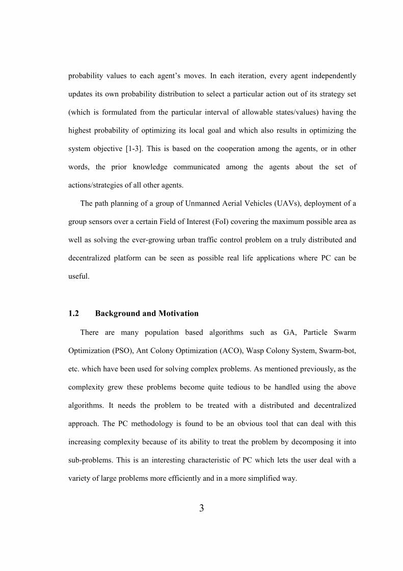
probability values to each agent’s moves. In each iteration, every agent independently

updates its own probability distribution to select a particular action out of its strategy set

(which is formulated from the particular interval of allowable states/values) having the

highest probability of optimizing its local goal and which also results in optimizing the

system objective [1-3]. This is based on the cooperation among the agents, or in other

words, the prior knowledge communicated among the agents about the set of

actions/strategies of all other agents.

The path planning of a group of Unmanned Aerial Vehicles (UAVs), deployment of a

group sensors over a certain Field of Interest (FoI) covering the maximum possible area as

well as solving the ever-growing urban traffic control problem on a truly distributed and

decentralized platform can be seen as possible real life applications where PC can be

useful.

1.2 Background and Motivation

There are many population based algorithms such as GA, Particle Swarm

Optimization (PSO), Ant Colony Optimization (ACO), Wasp Colony System, Swarm-bot,

etc. which have been used for solving complex problems. As mentioned previously, as the

complexity grew these problems become quite tedious to be handled using the above

algorithms. It needs the problem to be treated with a distributed and decentralized

approach. The PC methodology is found to be an obvious tool that can deal with this

increasing complexity because of its ability to treat the problem by decomposing it into

sub-problems. This is an interesting characteristic of PC which lets the user deal with a

variety of large problems more efficiently and in a more simplified way.

4

PC has been applied in variegated areas solving complex problems such as

optimization of mechanical structures [11]; airplane fleet assignment to a group of airports

minimizing the number of flights [12], collision avoidance [13], wireless sensor networks

[14-20], university course scheduling [21], etc. Moreover, the comparison between GA

and PC in [22] solving a variety of benchmark instances indicated the superiority of PC in

dealing with functions with important characteristics such as multimodality, nonlinearity

and non-separability.

Furthermore, Dr. Rodney Teo and Mr. Ye Chuan Yeo from the Cooperative Machines

Lab of DSO National Laboratories, Singapore were interested to solve path planning

problems for Multiple UAVs (MUAVs) by modeling them as Multiple Traveling

Salesmen Problems (MTSPs), with a possible extension towards a decentralized

optimization and control of these autonomous vehicles. This motivated the author of this

thesis to solve the MTSP by applying PC as a distributed and decentralized optimization

methodology.

In addition, the author of this thesis noticed the challenging area of the MTSP as one

where PC can be quite useful and show its potential. This is because the MTSP is a NP-

hard combinatorial optimization problem that, although easy to understand, remains a

challenge for researchers over the years. The MTSP is important because of its large

number of possible practical application areas such as logistics and manufacturing

scheduling [23, 24], delivery and pick-up scheduling [25-27], school bus delivery routing

[28, 29], satellite navigation systems [30], overnight security problem [31], etc.

Furthermore, the tools used for solving the MTSP such as PSO, ACO, GA, etc. are found

5

to be computationally expensive and have slow convergence. The related discussion can

be found in Chapter 4 of this thesis. This makes the PC to be seen as a promising option.

Most importantly, in the entire literature on PC, no generic constraint handling

technique was found to have been developed for incorporating into the overall PC

framework. Furthermore, having understood its potential in variegated areas and its ability

to deal with real world complex problems, a generic and powerful constraint handling

technique is required. This motivated the author to develop different constraint handling

techniques to incorporate into PC and further test them for solving a variety of constrained

problems.

In order to exploit this opportunity of testing the constraint handling techniques by

solving a variety of problems, the Circle Packing Problem (CPP) was chosen as it has a

great practical importance in production and packing for the textile, apparel, naval,

automobile, aerospace, food industries, etc. [32]. In addition, the CPP has received

considerable attention in the ‘pure’ mathematics literature but only limited attention in the

operations research literature [33].

Furthermore, the Sensor Network Coverage Problem (SNCP) was noticed to be one of

the most appropriate practical problems where the potential of constrained PC can be

tested. This is because the sensor network plays a significant role in various strategic

applications such as hostile and hazardous environmental and habitat exploration and

surveillance, critical infrastructure monitoring and protection, situational awareness of

battlefield and target detection, natural disaster relief, industrial sensing and diagnosis,

biomedical health monitoring, seismic sensing, etc. [34-42]. The deployment or

positioning of the individual sensor directly affects the coverage, detection capability,

6

connectivity and associated communication cost and resource management of the entire

network [36, 37, 43, 44]. According to [45], coverage is the important performance metric

that quantifies the quality and effectiveness of the surveillance/monitoring provided by the

sensor network. This highlighted the requirement of an effective sensor deployment

algorithm quantifying the coverage of the entire network [38, 43, 44].

In addition, the author of this thesis realizes the opportunity to explore various inherent

characteristics of PC methodology when solving different variations of the above

mentioned problems.

The next few subsections discuss the research objectives, the scope of the work as well

as the original contributions arising from this work while achieving the objectives.

1.3 Research Objectives

The following are the objectives of the current research work.

1. Extend the PC approach further in order to investigate and exploit its inherent and

desirable characteristics as well as key benefits of being a distributed, decentralized

and cooperative approach. This includes modifying the PC approach to make it more

efficient and faster.

2. Develop a more general and powerful approach of PC by incorporating constraint

handling techniques necessary for solving constrained optimization problems, and

further test and validate these techniques by solving a variety of challenging

constrained problems.

3. Solve the path planning problem of Multiple UAVs (MUAVs) by modeling it as a

MTSP and solving it by the PC approach.

7

1.4 Original Contributions Arising from this Work

Some of the objectives mentioned were accomplished and efforts are being made to

achieve those which are proposed. The original contributions arising from this work are

listed as follows:

1. Improvements to the original PC approach. The original PC approach was improved

with a reduction in the computational complexity. A scheme for updating the solution

space was developed which contributed to faster convergence and improved efficiency

of the overall algorithm. In addition, PC was assumed to be converged when there was

no further improvement in the final goal and/or when a predefined number of

iterations was exceeded. Moreover, in order to make the solution jump out of possible

local minima, a perturbation approach was developed and incorporated into the PC

approach.

2. Furthermore, in the efforts to make PC more generic and powerful, a number of

constraint handling techniques in the form of penalty function and feasibility-based

rules were developed for incorporating into the overall algorithm. This allowed PC to

solve practical problems which inevitably are constrained problems.

3. In the first attempt to develop a constraint handling technique, different problem

specific heuristics such as the node insertion heuristic and the node elimination

heuristic were proposed and incorporated into the PC algorithm for solving the NP-

hard problem such as the Multiple Traveling Salesmen Problem (MTSP). The

implementation of these techniques helped the algorithm to converge faster as well as

8

to jump out of local minima. In addition, in order to avoid the repeated sampling of the

nodes by vehicles, a simple sampling procedure was also developed and implemented.

4. For the first time, the MTSP was solved using a distributed, decentralized and

cooperative approach such as PC.

5. For the first time, the Circle Packing Problem (CPP) was solved using a distributed,

decentralized approach such as PC. It also helped to demonstrate the desirable and key

characteristic of a distributed approach to avoid the tragedy of commons.

6. For the first time, the important ability of PC to deal with the practically significant

subsystem failure or agent failure problem was demonstrated by solving a specially

designed case of the CPP incorporating agent failure.

7. Similar to the CPP and the MTSP, for the first time the Sensor Network Coverage

Problem (SNCP) was solved using a distributed, decentralized approach such as PC.

1.5 Scope of the Research Work

The thorough literature review on PC was done to understand and investigate the basic

concept of PC. The PC was modified and formulated. The modifications were done to

increase the efficiency as well as the performance.

The Rosenbrock Function (with limited number of variables) was solved to validate

the modified PC.

The further focus of the modification work was towards making the PC approach more

generic and powerful by developing different constraint handling techniques to

incorporate into the overall framework. In order to test the performance and viability of

the constrained PC, a variety of challenging and rigorous constrained problems were

9

solved. This further includes developing necessary techniques assisting the constraint

handling techniques.

The constrained PC was applied to two specially developed test problems (with

limited number of nodes and vehicles) for the Multiple Depot MTSP (MDMTSP) as well

as several randomly generated cases of the Single Depot MTSP (SDMTSP). To validate

the performance and efficiency of the approach, the results were compared with some

other algorithms solving the MTSP with approximately the same number of nodes and

vehicles.

Furthermore, the constrained PC was applied to solve several constrained test

problems available in the literature. The performance and efficiency of the solutions were

compared with the contemporary algorithms solving these problems.

Moreover, two specially developed cases of the Circle Packing Problem (CPP) with

limited number of circles were solved using the constrained PC approach. The

performance and efficiency of the solution were validated by solving these cases several

times with different initial configurations.

In addition to above, the constrained PC was applied to solve three specially

developed cases of the Sensor Network Coverage Problem (SNCP) with limited number

of sensors. Similar to the CPP, the performance and efficiency of the solution were

validated by solving the cases several times with different initial configurations.

Although PC is a distributed and decentralized approach, all the computations and

simulations were conducted on a single workstation.

10

1.6 Organization of the Thesis

The remainder of this thesis is organized as follows:

Chapter 2 provides the related literature, advantages and applications of the distributed,

decentralized and cooperative approach. It also highlights its importance in the field of

UAVs. Chapter 3 gives details of using PC in the COIN framework. It includes the

related work on PC, its characteristics, detailed formulation of modified unconstrained PC

approach and the formulation of the Nash equilibrium. It also provides the testing and

validation of the modified PC approach solving the Rosenbrock function. Chapter 4

discusses the early effort of incorporating the constraint handling technique into the PC

algorithm using problem specific heuristic techniques solving various cases of the

combinatorial optimization problem such as the MTSP. This chapter also includes detailed

discussed literature on MTSP as well as the literature on MUAVs path planning using the

MTSP approach. The effort of handling constraints by incorporating the penalty function

approach into the PC and solving a number of constrained test problems is described in

Chapter 5. Two variations of the constraint handling technique of Feasibility-based Rule

incorporated into the PC approach and solving several cases of the challenging Circle

Packing Problem (CPP) and Sensor Network Coverage Problem (SNCP) are described in

Chapter 6. Concluding remarks and recommendations for future work including other

potential constraint handling approaches as well as possible practical applications of PC

are discussed in Chapter 7. The necessary Appendices (A to D) are provided at the end

of the thesis.

11

CHAPTER 2

DISTRIBUTED, DECE�TRALIZED A�D COOPERATIVE

APPROACH

2.1 Distributed, Decentralized and Cooperative Approach

As mentioned previously, complex systems can be handled by decomposing them into

smaller subsystems. These systems can be optimized individually to attain the system

level optimum. This section discusses the literature related to the distributed, decentralized

and cooperative approach in order to underscore its superiority over the centralized

approach.

In a centralized system as shown in Figure 2.1, a single agent is supposed to have all

the capabilities, such as problem solving, in order to alleviate the user’s cognitive load.

The agent is provided with the general knowledge which is useful to do a wide variety of

tasks [46].

Figure 2.1: A Centralized System

Central

Agent

Tasks

12

This single agent needs enormous knowledge to deal effectively with the user requests;

it needs to do required computations and also needs enough storage space, etc. Such a

system may have a processing bottleneck. It also cannot be a robust system because of the

possibility of single point failure which may have serious impact. For example, the

process of information search over internet, information finding, filtering, etc. may

overwhelm a centralized system [47, 48]. On the other hand, if the work is divided or

decomposed into different tasks (e.g. information search, filtering, evaluation and

integration) by classifying the expertise needed in the system, the potential bottleneck can

be avoided. The classification of expertise here refers to the decomposition of the system

into various agents representing experts of the particular area in the system. This expertise

is the set of knowledge or actions the agent is supposed to have under the particular

circumstance. It is therefore natural to have a distributed Multi-Agent System (MAS)

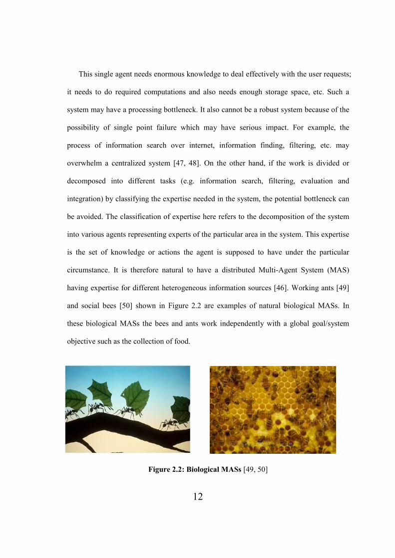
having expertise for different heterogeneous information sources [46]. Working ants [49]

and social bees [50] shown in Figure 2.2 are examples of natural biological MASs. In

these biological MASs the bees and ants work independently with a global goal/system

objective such as the collection of food.

Figure 2.2: Biological MASs [49, 50]

13

Furthermore, it is evident that such distributed, decentralized MAS is intended for

open-ended design problems where there is no well-defined solution available and

requires an in-depth search of the design space and also requires adaptability to user

preferences [48]. Designing a MAS to perform well on a collective platform is non-trivial.

Moreover, the straightforward agent learning in a MAS on collective platform cannot be

implemented as it can lead to a suboptimal solution and also may interfere with individual

interests [10]. This is referred to as ‘Tragedy of Commons’ in which the rational and self-

interested independent individuals deplete the shared limited resource in a greedy way,

even if it is well understood that it may not be beneficial for long term interest collectively

for all, i.e. an individual may receive a benefit but on the other hand the loss will be shared

among all [9]. This conflict may further lead to total system collapse. It also highlights the

inadequacy of the classic Reinforcement Learning (RL) approach. An attractive option is

to devise a distributed system in which different parts are referred to as agents; each

having local control, having cooperation among one another and contributing towards a

common aim. The cooperation among such agents is also important in order to avoid the

replication of the work and/or information and reduction in the computational load [46].

In the case of such cooperative distributed and decentralized system, there is also a

need for the right to share the information among the agents. It is important when dealing

with security/military systems, banking systems, construction systems, etc. When these

systems are used as centralized systems, the information from all the individual processes

need to be communicated to the centralized controller, planner, scheduler, etc. This can be

a hindrance when there may be some subsystems not willing to share the information with

14

the third party (or a centralized system). Such systems are very difficult to be optimized

centrally unless the right to share the information or right to cooperate is clearly defined.

The centralized approach is not suitable for the modern highly dynamic environment

as by the time the re-computation and re-distribution is done the environment is already

changed. This makes it clear that a centralized system may add latency in the overall

processing. On the other hand, the sub-problems can naturally be distributed and

decentralized into agents and on the basis of the inter-agent-cooperation, quicker decisions

can be taken and executed. According to [46, 47] autonomous agents perform

computations independently from other agents, and contribute their results in a parallel

and distributed fashion. Such collaborating agents make the system robust and flexible to

adapt easily to the user preference changes. It is also believed that the cooperating agents

in a distributed system collectively show better performance than a centralized system or a

distributed system with agents having absolutely no cooperation.

Furthermore, the major challenges addressed in the collective behavior of the

autonomous agents are how to enable the distributed agents to dynamically acquire their

goal-directed cooperative behavior in performing a certain task, and how to apply the

collective learning when addressing an ill-defined problem [51]. According to [46, 51-54],

the crucial step is to formulate and develop the structure and organize the agents in a MAS

ensuring achievement of the global optimum using the local knowledge. The other

challenges are how to ensure the robustness, how to impart adaptability, how to maintain

privacy, etc [55].

15

2.2 Advantages of the Distributed, Decentralized and Cooperative

Approach

The above approach is used in variegated applications because of its various

advantages. Some of the important advantages are discussed here.

1. It reduces the dependence on a single central system, thus reducing the chance of

single point failure. This imparts the important characteristic referred to as robustness.

This is essential in the field of UAV as failure of the centralized controller can be

devastating and may result in collision. This is addressed in the related work on UAVs

[2, 56-62].

2. It reduces computational overhead on a centralized system.

3. It reduces communication delays between resource agents and the coordinator as the

information is transferred to the corresponding agents rather than the central

system/agent [63]. It also solves the security issue such as sharing of information with

a centralized system [46] as the exchange of local information is allowed between the

entitled sub-systems/agents.

4. It allows the planning to be done on a shorter time scale, allowing additional

planning/coordination rounds to take place.

5. It reduces complexity of the coordination problem making the controllers simpler and

cheaper.

6. It reduces overall complexity of the problem formulation.

7. It imparts modularity and flexibility as one can reconfigure or expand the system by

adding new components, sub-systems in the realm of the problem and still the

16

computations can be carried out locally and no single system overload occurs [58, 64].

This feature is referred to as scalability.

8. As the computations are done at the local level, the system can be made more flexible

by dividing it into different problem solvers based on the abilities. This way the

decision making becomes faster by exploiting parallelism [65].

9. It enhances the local communication and subsequently reduces the overwhelming

energy consumption. According to [66], a sensor network communicating the raw data

to the central point uses more energy as compared to local communication in the

distributed approach.

10. The large and complex systems can be built into individual and simpler modules

which are easier to debug and maintain [63, 54].

11. It imparts reliability through redundancy [51].

12. It expedites the decision-making process by reducing latency [51, 54].

13. It helps to improve the real time response and behavior [31].

Some of the important applications exploiting the above advantages are discussed below.

2.3 Applications of the Distributed, Decentralized and Cooperative

Approach

The complex adaptive systems which work on distributed, decentralized and

cooperative MASs, because of their various advantages, have been successfully applied to

various engineering applications such as internet search, engineering design,

manufacturing, scheduling, logistics, sensor networks, vehicle routing, UAV path

17

planning and many more are currently being researched. Some of the applications are

discussed below.

Meta-heuristics is the field in which several search processes interchange the

information while searching the optimal solution. To have a successful search process, the

information exchange is very important. In case of a centralized system there is a central

agent that carries out the interchange of the information between the various processes. In

the decentralized cooperative system, each process has its own rules to decide when, what

and how to interchange the relevant information with the relevant processes [53]. This

approach of local communication reduces computational overload for the system, thus

speeding up further decision making. According to [53], logistics problems such as the

Vehicle Routing Problem (VRP), loading problem (Bin Packing) and location problem

can be solved using a decentralized cooperative way.

The information sources available online are inherently distributed and are having

different modalities. It is therefore natural to have a distributed MAS having expertise in

different heterogeneous information sources. The robustness of such a system is most

important because online information services are dynamic and unstable in nature. A

multi-agent computational infrastructure referred to as Reusable Task Structure-based

Intelligent Network Agents (Retsina) was proposed in [46]. This MAS searches

information on the internet, filters out irrelevant information, integrates information from

the heterogeneous sources and also updates the stored information in a distributed manner.

It is true that a sensor network communicating the raw data to the central point uses

more energy as compared to the distributed approach [67]. This forces undesirable limits

on the amount of information to be collected. This also imposes constraints on the amount

18

of information to be communicated as it affects communication overload. In the case of

distributed and decentralized sensor networks, each node is an individual solving the

problems independently and cooperatively. Similarly, the Radio Frequency Identification

(RFID) system proposed in [68] is a distributed and decentralized system in which a

subsystem or a sensor is not only a node collecting and transferring the data but also does

the processing and computing job in order to take decisions locally. These subsystems,

nodes or sensors are equipped with as much knowledge, logic, and rights as possible to

make it a better alternative to the centralized system.

In the approach presented in [69], the agents in MASs handle the pre- and post-

processing of various computational analysis tools such as spreadsheets or CAD systems

in order to have a common communication between them. These agents communicate

through a common framework where they act as experts and communicate their results to

the centralized design process. As the number of design components increase, the number

of agents and the complexity also increases. This results in the growing need for

communication, making it computationally cumbersome for a centralized system. This is

one of the reasons that the centralized approach is becoming insignificant in the

concurrent design.

The construction industries are becoming more complex and involving many

subcontractors. In a project, subcontractors perform most of the work independently and

manage their own resources. Their work affects the other subcontractors and eventually

the entire project. This makes it clear that the centralized system or control of such process

is inadequate to handle such situations. This suggests that the control needs to be

19

distributed into individual sub-contractors in order to reschedule their projects

dynamically [52].

A very different distributed MAS approach illustrated in [52] is the Distributed

Coordination Framework for Project Schedule Changes (DCPSC). The objective is the

minimization of the total extra cost each sub-contractor has to incur because of the abrupt

project schedule change. Every sub-contractor is assumed to be a software agent to

enhance communication using the internet. The agents in this distributed system compete

and take socially rational decisions to maintain a logical sequence of the network. As the

project needs to be rescheduled dynamically, extensive communication/negotiation among

the subcontractor agents is required. In this approach these agents interact with one

another to evaluate the impact of changes, simulate decisions in order to reduce the

possible individual loss.

There is a growing trend in many countries to generate and distribute power/energy

locally using renewable and non-conventional sources [70]. They are ‘distributed’ because

they are placed at or near the point of energy consumption, unlike traditional ‘centralized’

systems where electricity/energy is generated at a remotely located, large-scale power

plant and then transmitted down power lines to the consumer [71]. The same is true for the

distribution of heating and cooling systems [70]. Depending on the peak and non-peak

periods, the supply of energy has to be changed dynamically to accommodate the

unforeseen behavior and current demand characteristics.

The distributed and decentralized systems related to robotic systems need very high

robustness and flexibility. Examples of such applications are semi-automatic space

exploration [72], rescue [73], and underwater exploration [74]. The most common

20

technique to ensure the robustness in robotic systems is to decompose the complex system

into a distributed and decentralized system and also to introduce redundancy like that of

wireless networks [55, 63, 67] in which even though some nodes fail, the network

continues to operate [75]. Based on the experimentation, it is claimed that robotic

hardware redundancy is necessary along with distributed and decentralized control [76]. It

is worth to highlight that the self-reconfigurable robots such as MTRN [77] and PolyBot

[78] use centralized control despite a good hardware flexibility. As these robots are less

robust to failures, this disadvantage overwhelms flexibility.

Unmanned Vehicles (UVs) or Unmanned Aerial Vehicles (UAVs) are seen as flexible

and useful for many applications such as searching targets, mapping a given area, traffic

surveillance, fire monitoring, etc. [79]. They are very useful in the environment where the

use of manned airplane mission may be dangerous or impossible. UV/UAV is a strong

potential field in which decentralized and distributed approach can be applied for conflict

resolution, collision avoidance, better utilization of air-space and mapping efficient

trajectory. Some of these applications are discussed below.

The work demonstrated in [58] highlights the advantages of the distributed and

decentralized approach when applied to Air/Ground Traffic Management. Based on the

specialized job, the system is decomposed into three types of agents: airplanes/flight deck,

air traffic service provider and airline operational control. In the traditional approach of

Air/Ground Traffic Management the focus typically is on smooth, stable and orderly flow

of traffic at the expense of efficiency. The modern concept of free flight presented in [58],

avoids the latency in decision making in highly dense traffic conditions. If the planned

trajectories are in conflict zone with one another the corresponding airplanes change the

21

trajectories without communicating to the centralized system, avoiding communication

overhead and further delay in the decision. This makes the centralized system insignificant

keeping the communication to local level. Such decentralized control strategy reduces

conflict alerts (crisis) as well.

In the dynamic environment of a war field, the risk or potential threats change their

positions with respect to time. The objective of the UAVs is to reach a particular point at

the same time following the shortest path. The Probabilistic Map approach was proposed

in [80], in which based on the local information and/or positions of the threats the local

updating of the terrain map was done and was directly communicated with the

neighboring UAVs. This cooperation helped real time updating of the map and also

decentralized and distributed control by each airplane was possible. A similar approach

could also be seen in the sensor networks to find out the location of the airplane [54] in

which different nodes positioned topographically at different locations monitor the same

aircraft but the perception of each node is different. This does not necessarily provide

information about the aircraft movement/location unless the information gathered by all

these sensors is integrated and communicated to neighboring nodes to produce an overall

picture of aircraft movements, i.e. the overall solution.

The problem of UAVs formation following a stationary/moving target was addressed

in [60]. In the formation, each UAV tries to keep a desired distance from the neighboring

one. It was claimed that forming the objective function controlling all the UAVs in the

flock showing the formation instincts such as collision avoidance, obstacle avoidance,

formation keeping, etc. is non-trivial. Also, dealing with such single objective function is

computationally expensive. This becomes worse when the formation tries to add more

22

UAVs. In [60], each aircraft was modeled separately for collision avoidance, formation

keeping, target seeking, obstacle avoidance, etc. A similar approach was implemented by

[61] for a fleet of Multiple UAVs (MUAVs). In this model, gyroscopic force was used to

change the direction of individual airplanes to avoid possible collisions. In both of these

proposed works, as each vehicle has local control and computations, the system shows

high scalability to include a large number of vehicles in the fleet. Similar to this,

computationally Distributed, Decentralized Optimization for Cooperative Control of

Multi-agent Swarm-like Systems was proposed in [81].

The number of potential conflicts grows exponentially as the number of vehicles

grows. This highlights the insignificance of centralized approach and shows the need for a

distributed and decentralized control approach. The space under consideration may get

added with more vehicles, increasing the possibility of conflict. This problem was handled

by developing a model of field sensing approach having attraction towards the target and

repulsion to the obstacle or neighboring vehicle in [66]. Each UAV was modeled as a

magnetic dipole and was provided with a sensor to detect the magnetic field generated by

other UAVs estimating the gradient. This estimate was used to go in the opposite direction

to avoid conflict. There was absolutely no cooperation among the UAVs. The complex

system such as airplane fleet assignment was also implemented successfully in [12]. It is

discussed in the next chapter on Probability Collectives (PC).

The PC methodology in COIN framework through which the distributed, decentralized

and cooperative optimization can be implemented is discussed in detail in the following

chapter.

23

CHAPTER 3

COLLECTIVE I�TELLIGE�CE USI�G PC

An emerging Artificial Intelligence tool in the framework of Collective Intelligence

(COIN) for modeling and controlling distributed MAS referred to as Probability

Collectives (PC) was first proposed by Dr. David Wolpert in 1999 in a technical report

presented to NASA [1]. It is inspired from a sociophysics viewpoint with deep

connections to Game Theory, Statistical Physics, and Optimization [3, 4]. From another

viewpoint, the method of PC theory is an efficient way of sampling the joint probability

space, converting the problem into the convex space of probability distribution. PC

considers the variables in the system as individual agents/players in a game being played

iteratively [2, 12, 11]. Unlike stochastic approaches such as Genetic Algorithm (GA),

Swarm Optimization or Simulated Annealing (SA), rather than deciding on the agent’s

moves/set of actions, PC allocates the probability values for selecting each of the agent’s

moves. At each iteration, every agent independently updates its own probability

distribution over a strategy set which is the set of moves/actions affecting its local goal

which in turn also affects the global or system objective [3]. The process continues and

reaches equilibrium when no further increase in reward is possible for the individual agent

by changing its actions further. This equilibrium concept is referred to as Nash

equilibrium [5]. The concept is successfully formalized and implemented through the PC

methodology. The approach works on probability distributions, directly incorporating

uncertainty and is based on prior knowledge of the actions/strategies of all the other agents.

The literature on PC is discussed in the following section.

24

3.1 Literature Review of PC

The approach of PC has been implemented for solving the problems from variegated

areas [6-8, 10-22, 82-88]. The associated literature is discussed in the following few

paragraphs.

It was demonstrated in [86] optimizing the Schaffer's function that the search process in

PC is more robust/reproducible as compared to GA. In addition, PC also outperformed GA

in the rate of descent, trapping in false minima and long term optimization when tested

and compared for the multimodality, nonlinearity and non-separability in solving other

benchmark problems such as Schaffer's function, Rosenbrock function, Ackley Path

function and Michalewicz Epistatic function. Some of the fundamental differences

between GA and PC were also discussed in [22]. At the core of the GA optimization

algorithm is the population of solutions. In every iteration, each individual solution from

the population is tested for its fitness to the problem at hand [22] and the population is

updated accordingly. GA plots the best-so-far curve showing the fitness of the best

individual in the last preset generations. In PC, on the other hand, the probability

distribution of the possible solutions is updated iteratively. After a predefined number of

iterations, the probability distribution of the available strategies across the variable space

is plotted in PC when optimizing an associated Homotopy function. It also directly

incorporates uncertainty due to both imperfect sampling and the stochastic independence

of the agents' actions [22]. Furthermore, PC outperformed the Heuristic Adaptive GA

(HAGA) [89], Heuristic ACO (HACO) [90] and Heuristic PSO (HPSO) [91] in stability

and robustness solving the air combat decision-making for coordinated multiple target

25

assignment problem [87]. The above comparison indicated that PC can potentially be

applied to wide application areas.

The superiority of the decentralized PC architecture over a centralized one was

underlined in [10] when solving the 8-queens problem. Both the approaches differ from

each other because of the distributed sample generation and updating of the probabilities

in the former approach. In addition, PC was also compared with the backtracking

algorithm referred to as Asynchronous Distributed OPTimization (ADOPT) [92].

Although the ADOPT algorithm is a distributed approach, the communication and

computational load was not equally distributed among the agents. It was also

demonstrated that although ADOPT was guaranteed to find the solution in each run,

communication and computations required were more than for the same problem solved

using PC.

The approach of PC was successfully applied in solving the complex combinatorial

optimization problem of airplane fleet assignment having the goal of minimization of the

number of flights with 129 variables and 184 constraints. Applying a centralized approach

to this problem may increase the communication and computational load. Furthermore, it

may add latency in the system and result in the growing possibility of conflict in schedules

and continuity. Using PC, the goal was collectively achieved by exploiting the advantages

of a distributed and decentralized approach by the airplanes selecting their own schedules

depending upon the individual payoffs for the possible routes [12].

The potential of PC in mechanical design was demonstrated for optimizing the cross-

sections of individual bars and segments of a 10 bar truss [11]. The problem was

formulated as a discrete problem and the solution was feasible but was worse than those

26

obtained by other methods [93-95]. The approach of PC [11, 12] was also tested on the

discrete problem of university course scheduling [21], but the implementation failed to

generate any feasible solution. It is important to note that although the problems in [11, 12,

21] are constrained problems, the constraints were not explicitly treated or incorporated in

the PC algorithms.

Very recently, two different PC approaches were proposed in [13] solving an

autonomous conflict resolution problem for cooperating airplanes to avoid the mid-air

collision. In the first approach, every airplane was assumed to be an autonomous agent.

These agents selected their individual paths and avoided collision with other airplanes

traveling in the neighborhood. In order to implement this approach, a complex negotiation

mechanism was required for the airplanes to communicate and cooperate with one another.

In the second approach which is a semicentralized approach, every airplane was given a

chance to become a host airplane which computed and distributed the solution to all other

airplanes. It is important to mention that the host airplane computed the solution based on

the independent solution shared by previous host airplane. This process continued in a

sequence until all the airplanes selected their individual paths. Both the approaches were

validated solving an interesting airplane conflict resolution problem in which the airplanes

were equidistantly arranged on the periphery of a circle. The targets of the individual

airplanes were set as the opposite points on the periphery of the circle, setting the center

point of the circle as a point of conflict. In both the approaches, collision constraints were

molded into special penalty functions which were further integrated into the objective

function using suitable balancing factors. Similar to the weighted sum multi-objective

27

approach [96, 97], the balancing factors were assigned based on the importance of the

corresponding constraints.

A variation of the original PC approach in [1-4, 11, 12] referred to as Sequentially

Updated PC (SPC) was proposed in [88]. The variation was achieved by changing the

sampling criterion and the method for estimating the sampling space in every iteration.

The SPC was tested by optimizing the unconstrained Hartman’s functions and the vehicle

target assignment type of game. The SPC performed better with higher dimension

Hartman’s functions only but failed to converge in the target assignment game. The

approach of PC was also successfully applied in solving combinatorial optimization

problems such as the joint optimization of the routing and resource allocation in wireless

networks [14-20].

3.2 Characteristics of PC

The PC approach has the following key characteristics that make it a competitive choice

over other algorithms for optimizing collectives.

1. PC is a distributed solution approach in which each agent independently updates its

probability distribution at any time instance and can be applied to continuous, discrete

or mixed variables, etc. [3, 1, 11, 12]. Since the probability distribution of the strategy

set is always a vector of real numbers regardless of the type of variable under

consideration, conventional techniques of optimization for Euclidean vectors, such as

gradient descent, can be exploited.

2. It is robust in the sense that the cost function (global/system objective) can be irregular

or noisy, i.e. it can accommodate noisy and poorly modeled problems [3, 10].

28

3. The failed agent can just be considered as one that does not update its probability

distribution, without affecting the other agents. On the other hand, it may severely

hamper the performance of other techniques [10].

4. It provides the sensitivity information about the problem in the sense that a variable

with a peaky distribution (having highest probability value) is more important in the

solution than a variable with a broad distribution, i.e. peaky distribution provides the

best choice of action that can optimize the global goal [3].

5. The formation of the Homotopy function for each agent (variable) helps the algorithm

to jump out of the possible local minima and further reach the global minima [12, 7, 8,

85].

6. It can successfully avoid the tragedy of commons, skipping the local minima and

further reach the true global minima [10].

7. The computational and communication load is marginally less and equally distributed

among all the agents [10].

8. It can efficiently handle problems with a large number of variables [12].

With PC solving optimization problems as a MAS, it is worth discussing some of its

characteristics to compare the similarities and differences with Multi-Agent

Reinforcement Learning (MARL) methods. Most MARL methods such as fully

cooperative, fully competitive and mixed (neither cooperative nor competitive) are based

on Game Theory, Optimization and Evolutionary Computation [98]. According to [98],

most of these types of methods possess less scalability and are sensitive to imperfect

observations. Any uncertainty or incomplete information may lead to unexpected behavior

of the agents. However, the scalability of the fully cooperative methods such as

29

coordination free methods can be enhanced by explicitly using the communication and/or

uncertainty techniques [98-101]. On the other hand, PC is scalable and can handle

uncertainty in terms of probability. Moreover, the random strategies selected by any agent

can be coordinated or negotiated with the other agents based on the social conventions,

right to communication, etc. This social aspect makes PC a cooperative approach.

Furthermore, indirect coordination based methods work on the concept of biasing the

selection towards the likelihood of the good strategies. This concept is similar to the one

used in the PC algorithm presented here, in which agents choose the strategy sets only in

the neighborhood of the best strategy identified in the previous iteration. In the case of

mixed MARL algorithms, the agents have no constraints imposed on their rewards. It is

similar to the PC algorithm in which the agents respond or select the strategies and exhibit

self-interested behavior. However, the mixed MARL algorithms may encounter multiple

Nash Equilibria while in PC a unique Nash equilibrium can be achieved.

3.3 Conceptual Framework of PC

PC treats the variables in an optimization problem as individual self interested learning

agents/players of a game being played iteratively [11, 12]. While working in some definite

direction, these agents select actions over a particular interval and receive some local

rewards on the basis of the system objective achieved because of those actions. In other

words, these agents optimize their local rewards or payoffs, which also optimize the

system level performance. The process iterates and reaches equilibrium (referred to as

Nash equilibrium) when no further increase in the reward is possible for the individual

agent through changing its actions further. Moreover, the method of PC theory is an

30

efficient way of sampling the joint probability space, converting the problem into the

convex space of probability distribution. PC allocates probability values to each agent’s

moves, and hence directly incorporates uncertainty. This is based on prior knowledge of

the recent action or behavior selected by all other agents. In short, the agents in the PC

framework need to have knowledge of the environment along with every other agent’s

recent action or behavior.

In every iteration, each agent randomly samples from within its own strategy set as

well as from within other agents’ strategy sets and computes the corresponding system

objectives. The other agents’ strategy sets are modeled by each agent based on their recent

actions or behavior only, i.e. based on partial knowledge. By minimizing the collection of

system objectives, every agent identifies the possible strategy which contributes the most

towards the minimization of the collection of system objectives. Such a collection of

functions is computationally expensive to minimize and also may lead to local minima [2].

In order to avoid this difficulty, the collection of system objectives is deformed into

another topological space forming the Homotopy function parameterized by

computational temperature T [102-105]. Due to its analogy to Helmholtz free energy [2,

4, 102-106], the approach of Deterministic Annealing (DA) converting the discrete

variable space into continuous variable space of probability distribution is applied in

minimizing the Homotopy function. At every successive temperature drop, the

minimization of the Homotopy function is carried out using a second order optimization

scheme such as the Nearest Newton Descent Scheme [1-4, 6, 10-22, 82-89] or BFGS

Scheme [7, 8], etc.

31

At the end of every iteration, each agent i converges to a probability distribution

clearly distinguishing the contribution of its every corresponding strategy value. For every

agent, the strategy value with the maximum probability value is referred to as the

favorable strategy and is used to compute the system objective. The solution is accepted

only if the associated system objective and corresponding strategy values are not worse

than the previous iterations solution. In this way, the algorithm continues until

convergence by selecting the samples from the neighborhood of the recent favorable

strategies.

In some of the applications, the agents are also needed to provide the knowledge of the

inter-agent-relationship. It is one of the information/strategy sets which every other

entitled agent is supposed to know. There is also global information that every agent is

supposed to know. This allows agents to know the right to model other agents’ actions or

behavior. All of the decisions are taken autonomously by each agent considering the

available information in order to optimize the local goals and hence to achieve the

optimum global goal or system objective.

The following section describes the detailed formulation of the PC procedure as an

unconstrained approach.

3.4 Formulation of Unconstrained PC

Consider a general unconstrained problem (in minimization sense) comprising !

variables and objective function G . In the context of PC, the variables of the problem are

considered as computational agents/players of a social game being played iteratively [1, 2].

32

Each variable, i.e. each agent i is given a predefined sampling interval referred to as

,lower upper

i i i Ψ ∈ Ψ Ψ . As a general case, the interval can also be referred to as the

sampling space. The lower limit lower

iΨ and upper limit upper

iΨ of the interval iΨ may be

updated iteratively as the algorithm progresses.

Each agent i randomly samples [ ]r

iX , 1, 2,..., ir m= strategies from within the

corresponding sampling interval iΨ forming a strategy set

iX represented as

[ ][1] [2] [3]{ , , , ..., }im

i i i i iX X X X=X , 1,2,...,i != (3.1)

Every agent is assumed to have an equal number of strategies, i.e.

1 2 1... ...i ! !m m m m m−= = = = = = . The procedure of modified PC theory is explained

below in detail with the algorithm flowchart in Figure 3.1.

The procedure begins with the initialization of the sampling interval iΨ for each agent

i , temperature 0T >> or initialT T= or T →∞ (simply high enough), the temperature step

size Tα ( 0 1Tα< ≤ ), convergence parameter 0.0001ε = , interval factor

downλ and

algorithm iteration counter 1n = . The value of Tα ,

im and downλ are chosen based on

preliminary trials of the algorithm.

Step 1. Agent i selects its first strategy [ ]1

iX . Agent i then samples randomly from other

agents’ strategies as well. These are random guesses by agent i about which

strategies have been chosen by the other agents. All these form a ‘combined

strategy set’ [ ]1

iY given by

{ }[1] [?] [?] [1] [?] [?]

1 2 1, ,..., ,..., ,i i ! !X X X X X−=Y (3.2)

33

The superscript [?] indicates that it is a ‘random guess’ and not known in advance.

In addition, agent i forms one combined strategy set for each of the remaining

strategies of its strategy set iX (i.e. 2,3,..., ir m= ), as shown below.

{ }{ }

{ }

{ }

[2] [?] [?] [2] [?] [?]

1 2 1

[3] [?] [?] [3] [?] [?]

1 2 1

[ ] [?] [?] [ ] [?] [?]

1 2 1

[ ] [ ][?] [?] [?] [?]

1 2 1

, ,..., ,..., ,

, ,..., ,..., ,

, ,..., ,..., ,

, ,..., ,..., ,i i

i i ! !

i i ! !

r r

i i ! !

m m

i i ! !

X X X X X

X X X X X

X X X X X

X X X X X

−

−

−

−

=

=

=

=

Y

Y

Y

Y

⋮

⋮

(3.3)

Similarly, all the remaining agents form their combined strategy sets.

Furthermore, every agent i computes im associated objective function values

as follows:

( ) ( ) ( ) ( )[ ][1] [2] [ ], ,..., ,..., imr

i i i iG G G G Y Y Y Y (3.4)

The ultimate goal of every agent i is to identify its strategy value which

contributes the most towards the minimization of the sum of these system

objective values, i.e. [ ]

1

( )im

r

i

r

G=∑ Y , hereafter referred to as the collection of system

objectives.

Step 2. The minimum of the function [ ]

1

( )im

r

i

r

G=∑ Y is very hard to achieve as the function

may have many possible local minima. Moreover, directly minimizing this

function is quite cumbersome as it may need excessive computational effort [2].

One of the ways to deal with this difficulty is to deform the function into another

topological space by constructing a related and ‘easier’ function ( )if X . Such a

34

method is referred to as the Homotopy method [102-105]. The function ( )if X

can be referred to as ‘easier’ because it is easy to compute, the (global) minimum

of such a function is known and easy to locate [102-104]. The deformed function

can also be referred to as Homotopy function J parameterized by computational

temperature T represented as follows:

( )( ) ( )[ ]

1

, ( )im

r

i i i i

r

J q T G T f=

= −∑X Y X , [ )0,T ∈ ∞ (3.5)

The approach of Deterministic Annealing (DA) is applied to minimize the

Homotopy function in equation (3.5). The motivation behind this is its analogy to

the Helmholtz free energy [6-8, 85, 106]. It suggests the conversion of discrete

variables into random real valued variables such as probabilities. This converts

the original collection of system objectives [ ]

1

( )im

r

i

r

G=∑ Y into the ‘expected

collection of system objectives’ ( )[ ]

1

( )im

r

i

r

E G=∑ Y . Furthermore, a suitable function

for ( )if X is chosen. The general choice is to use the entropy function

[ ] [ ]

2

1

S ( ) log ( )im

r r

i i i

r

q X q X=

= −∑ [101-103]. The following steps of DA are

formulated based on the analogy of the Homotopy function to the Helmholtz free

energy [6-8, 85, 106] discussed in Appendix A.

35

Figure 3.1: Unconstrained PC Algorithm Flowchart

START

Initialize n , T , Tα , downλ and sampling interval iΨ for every agent i . For every

agent i set up strategy set iX with im strategies

Form combined strategy set [ ]riY for every strategy r of agent i and compute objective

function [ ]( )r

iG Y

Assign uniform probabilities for every agent strategies, i.e. [ ]: ( ) 1/

riir q X m∀ = and

compute expected collection of system objectives ( )[ ]

1

( )im

r

i

r

E G=∑ Y

Form the modified Homotopy function ( )( )J ,i i

q TX

Minimize the Homotopy function using second order optimization technique such as

Nearest Newton method or BFGS method

Obtain the probability distribution ( )iq X for every agent i clearly distinguishing every

corresponding strategy’s contribution and identifying every agent’s favorable strategy

[ ]fav

iX

For each agent i , apply downλ

to update the sampling interval

iΨ and form corresponding

updated strategy set iX

Current obj. fun

≤ Previous obj.

fun

Accept current objective function

[ ]( )

favG Y and related favorable

strategies [ ]favY

N

Discard current [ ]( )fav

G Y and retain

previous [ ]( )

favG Y and related

favorable strategies [ ]favY

STOP

Accept [ ]( )fav

G Y as

[ ]( )

fav finalG Y along with

related [ ]favY

Convergence?

1n n= + , TT T Tα= −

Y

Y N

Compute the objective function [ ]( )

favG Y

36

(a) Agent i assigns uniform probabilities to its strategies. This is because, at the

beginning, the least information is available (the largest uncertainty and highest

entropy) about which strategy is favorable for the minimization of the collection

of system objectives [ ]

1

( )im

r

i

r

G=∑ Y . Therefore, at the beginning of the ‘game’, each

agent’s every strategy has probability 1/ im of being most favorable. Therefore,

probability of strategy r of agent i is

[ ]( ) 1 /r

i iq X m= , 1, 2,..., ir m= (3.6)

Each agent i , from its every combined strategy set [ ]r

iY and corresponding

system objective [ ]( )r

iG Y computed previously, further computes im

corresponding expected system objective values ( )[ ]( )

r

iE G Y as follows [1-4, 11,

12]:

( )[ ] [ ] [ ] [?]

( )

( )

( ) ( ) ( ) ( )r r r

i i i i

i

E G G q X q X= ∏Y Y (3.7)

where ( )i represents every agent other than i . Every agent i then computes the

expected collection of system objectives denoted by ( )[ ]

1

( )im

r

i

r

E G=∑ Y . It also

means that the PC approach can convert any discrete variables into continuous

variable values in the form of probabilities corresponding to these discrete

variables. As mentioned earlier, the problem now becomes continuous but still not

easier to solve.

(b) Thus the Homotopy function to be minimized by each agent i in equation (3.5) is

developed as follows:

37

( )( ) ( )[ ]

1

[ ] [ ] [?] [ ] [ ]

( ) 2

1 1( )

[1] [1] [?] [2] [2] [?]

( ) ( )

( ) ( )

[ 1] [ 1]

, ( ) S

( ) ( ) ( ) ( ) log ( )

( ) ( ) ( ) (Y ) ( ) ( ) ...

... ( ) ( ) (

i

i i

i i

mr

i i i i

r

m mr r r r

i i i i i

r ri

i i i i i i

i i

m m

i i

J q T E G T

G q X q X T q X q X

G q X q X G q X q X

G q X q X

=

= =

− −

= −

= − −

= + +

+

∑

∑ ∑∏

∏ ∏

X Y

Y

Y

Y[ ] [ ][?] [?]

( ) ( )

( ) ( )

[ ] [ ]

2

1

) (Y ) ( ) ( )

( ) log ( )

i i

i

m m

i i i i

i i

mr r

i i

r

G q X q X

T q X q X=

+

− −

∏ ∏

∑

(3.8)

where [ )0,T ∈ ∞ . When the temperature T is high enough, the entropy term

dominates the expected collection of system objectives and the problem becomes

very easy to be solved.

Step 3. The minimization of the Homotopy function in (3.8) can be carried out using

Nearest Newton Descent Scheme [1-4, 6, 10-22, 82-89] as well as a suitable

second order optimization approach such as Broyden-Fletcher-Goldfarb-Shanno

(BFGS) scheme [7, 96, 97]. The Nearest Newton Descent Scheme and the BFGS

scheme minimizing equation (3.8) are discussed in Appendix B and Appendix C,

respectively.

Step 4. For each agent i , the optimization process converges to a probability variable

vector ( )iq X which can be seen as the individual agent’s probability distribution

distinguishing every strategy’s contribution towards the minimization of the

expected collection of system objectives ( )[ ]

1

( )im

r

i

r

E G=∑ Y . In other words, for each

agent i , if a particular strategy r contributes the most towards the minimization

of the objective compared to other strategies, its corresponding probability

certainly increases by some amount more than those for the other strategies’

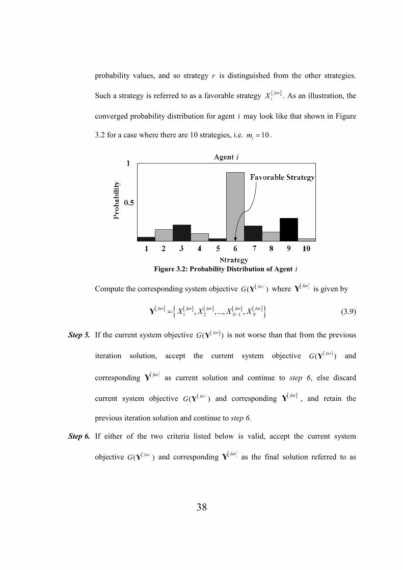
38

probability values, and so strategy r is distinguished from the other strategies.

Such a strategy is referred to as a favorable strategy [ ]fav

iX . As an illustration, the

converged probability distribution for agent i may look like that shown in Figure

3.2 for a case where there are 10 strategies, i.e. 10im = .

Figure 3.2: Probability Distribution of Agent i

Compute the corresponding system objective [ ]( )fav

G Y where [ ]fav

Y is given by

[ ] [ ] [ ] [ ] [ ]{ }1 2 1, ,..., ,fav fav fav fav fav

! !X X X X−=Y (3.9)

Step 5. If the current system objective [ ]( )fav

G Y is not worse than that from the previous

iteration solution, accept the current system objective [ ]( )fav

G Y and

corresponding [ ]fav

Y as current solution and continue to step 6, else discard

current system objective [ ]( )fav

G Y and corresponding [ ]fav

Y , and retain the

previous iteration solution and continue to step 6.

Step 6. If either of the two criteria listed below is valid, accept the current system

objective [ ]( )fav


Y as the final solution referred to as

i

39

[ ],( )fav final

G Y and [ ] [ ] [ ] [ ] [ ]{ }, , , , ,

1 2 1, ,..., ,fav final fav final fav final fav final fav final

! !X X X X−=Y ,

respectively and stop, else continue to step 7.

(a) If temperature finalT T= or 0T → .

(b) If there is no significant change in the system objectives for successive

considerable number of iterations (i.e. [ ] [ ], , 1

( ) ( )fav n fav n

G G ε−− ≤Y Y ).

Step 7. Every agent shrinks its sampling interval as follows:

[ ]( ) [ ]( ),fav favupper lower upper lower

i i down i i i down i iX Xλ λ Ψ ∈ − Ψ −Ψ + Ψ −Ψ , 0 1downλ< ≤

(3.10)

where downλ is referred to as the interval factor corresponding to the shrinking of

sample space.

Each agent i then samples im strategies from within the updated sampling

interval iΨ and forms the corresponding updated strategy set

iX represented as

follows.

[ ][1] [2] [3]{ , , , ..., }im

i i i i iX X X X=X , i 1,2,..., != (3.11)

Reduce the temperature TT T Tα= − , update the iteration counter 1n n= + and

return to step 1.

On convergence, the above process reaches the equilibrium referred to as Nash

equilibrium. The concept and detailed formulation of the Nash equilibrium achieved is

described in the following section.

40

3.5 �ash Equilibrium

To achieve a Nash equilibrium, every agent in a MAS should have the properties of

Rationality and Convergence [98-101]. Rationality refers to the property by which every

agent selects (or converges to) the best possible strategy given the strategies of the other

agents. The convergence property refers to the stability condition i.e. a policy using which

every agent selects (or converges to) the best possible strategy when all the other agents

use their policies from a predefined class (preferably same class). The Nash equilibrium is

naturally achieved when all the agents in a MAS are convergent and rational. Moreover, a

Nash equilibrium is guaranteed when all the agents use stationary policies, i.e. those

policies that do not change over time. It is worth to mention here that all the agents in the

MAS proposed using PC algorithm exhibit the above mentioned properties. For example,

as detailed in the PC algorithm discussed in the previous few paragraphs, there is a fixed

framework by which the agents select their own strategies and guess the other agents’

strategies.

In any game, there may be a large but finite number of Nash equilibria present,

depending on the number of strategies per agent as well as the number of agents. It is

essential to choose the best possible combination of the individual strategies selected by

each agent. It is computationally prohibitive to go through every possible combination of

the individual agent strategies and choose the best out of it that can produce a best

possible Nash equilibrium and hence the system objective.

As discussed in the detailed PC algorithm, in each iteration n , every agent i selects the

best possible strategy referred to as the favorable strategy [ ],fav n

iX by guessing the possible

strategies of the other agents. This information about its favorable strategy [ ],fav n

iX is made

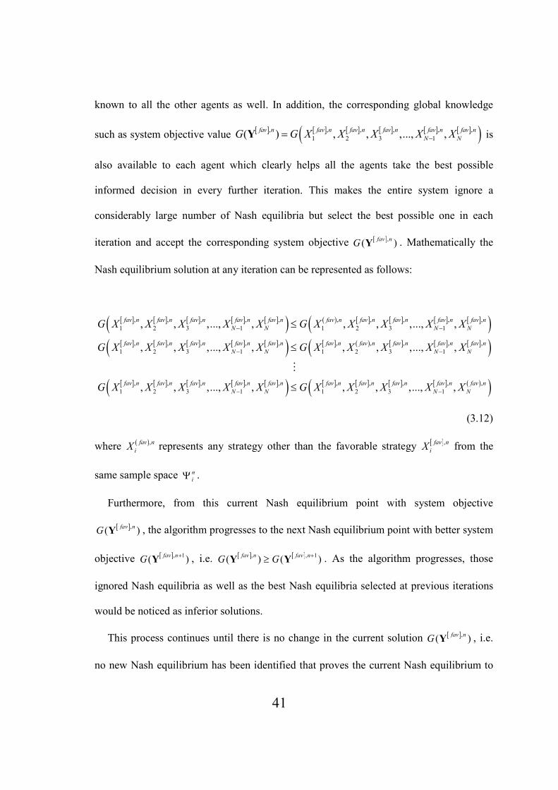
41

known to all the other agents as well. In addition, the corresponding global knowledge

such as system objective value [ ] [ ] [ ] [ ] [ ] [ ]( ), , , , , ,

1 2 3 1( ) , , ,..., ,fav n fav n fav n fav n fav n fav n

! !G G X X X X X−=Y is

also available to each agent which clearly helps all the agents take the best possible

informed decision in every further iteration. This makes the entire system ignore a

considerably large number of Nash equilibria but select the best possible one in each

iteration and accept the corresponding system objective [ ],( )fav n

G Y . Mathematically the

Nash equilibrium solution at any iteration can be represented as follows:

[ ] [ ] [ ] [ ] [ ]( ) ( ) [ ] [ ] [ ] [ ]( )[ ] [ ] [ ] [ ] [ ]( ) [ ] ( ) [ ] [ ] [ ]( )

[ ]

, , , , , , , , ,,

1 2 3 1 1 2 3 1

, , , , , , , , ,,

1 2 3 1 1 2 3 1

,

1 2

, , ,..., , , , ,..., ,

, , ,..., , , , ,..., ,

,

fav n fav n fav n fav n fav n fav n fav n fav n fav nfav n

! ! ! !

fav n fav n fav n fav n fav n fav n fav n fav n fav nfav n

! ! ! !

fav n fa

G X X X X X G X X X X X

G X X X X X G X X X X X

G X X

− −

− −

≤

≤

⋮

[ ] [ ] [ ] [ ]( ) [ ] [ ] [ ] [ ] ( )( ), , , , , , , , ,

3 1 1 2 3 1, ,..., , , , ,..., ,v n fav n fav n fav n fav n fav n fav n fav n fav n

! ! ! !X X X G X X X X X− −≤

(3.12)

where ( ),fav n

iX represents any strategy other than the favorable strategy [ ],fav n

iX from the

same sample space n

iΨ .

Furthermore, from this current Nash equilibrium point with system objective

[ ],( )fav n

G Y , the algorithm progresses to the next Nash equilibrium point with better system

objective [ ], 1( )

fav nG

+Y , i.e. [ ] [ ], , 1

( ) ( )fav n fav n

G G+≥Y Y . As the algorithm progresses, those

ignored Nash equilibria as well as the best Nash equilibria selected at previous iterations

would be noticed as inferior solutions.

This process continues until there is no change in the current solution [ ],( )fav n

G Y , i.e.

no new Nash equilibrium has been identified that proves the current Nash equilibrium to

42

be inferior. Hence the system exhibits stage-wise convergence to a unique Nash

equilibrium and the corresponding system objective is accepted as the final solution

[ ],( )

fav finalG Y . As a general case, this progress can be represented as follows:

[ ] [ ] [ ] [ ] [ ],1 ,2 , , 1 ,( ) ( ) ... ( ) ( ) ... ( )

fav fav fav n fav n fav finalG G G G G

+≥ ≥ ≥ ≥ ≥ ≥Y Y Y Y Y .

It is worth to mention some of the key differences of the PC methodology presented

here and the original PC approach [1-3, 11, 12]. In the present approach, fewer numbers of

samples were drawn from the uniform distribution of the individual agent’s sampling

interval. On the contrary, the original PC approach [1-3, 11, 12] used a Monte Carlo

sampling method which was computationally expensive and slow as the number of

samples needed was in the thousands or even millions. Most significantly, the sampling in

further stages of the PC algorithm presented here was narrowed down in every iteration by

selecting the sampling interval in the neighborhood of the most favorable value in the

particular iteration. This ensures faster convergence and an improvement in efficiency

over the original PC approach in which regression was necessary to sample the strategy

values in the close neighborhood of the favorable value.

3.6 Validation of the Unconstrained PC

There are a number of benchmark test functions for contemporary optimization

algorithms like GAs and evolutionary computation. The Rosenbrock function is an

example of a nonlinear function having strongly coupled variables and is a real challenge

for any optimization algorithm because of its slow convergence for most optimization

methods [107, 108]. The Rosenbrock function with ! number of variables is given by

43

( ) ( )1

2 22

1

1

100 1!

i i i

i

G x x x−

+=

= − + − ∑ (3.13)

lower limit upper limit, 1, 2,...,ix i !≤ ≤ =

and the global minimum is at, 1, 1, 2,...,ix i i != ∀ = , where * 0G = . A difficulty arises

from the fact that the optimum is located in a deep and narrow parabolic valley with a flat

bottom. Also, gradient based methods may have to spend a large number of iterations to

reach the global minimum.

In the context of PC, every function variable , 1, 2,...,ix i != was represented as an

autonomous agent. These agents competed with one another to optimize their individual

values and ultimately the entire function value (i.e. global objective G ). The Rosenbrock

function with 5 variables/agents ( 5! = ) was solved here in which each agent randomly

selected the strategies from within a predefined sampling interval iΨ . Although the

optimal value of each and every agent ix is 1, the allowable sampling interval

iΨ for each

agent was intentionally assigned to be different (as shown in Table 3.1). The procedure

explained in Section 3.4 was followed to reach convergence. For all the trials, the

temperature step size Tα , the interval factor

downλ and sample size im for each agent

chosen were 0.9, 0.1 and 42, respectively. It is worth to mention that the temperature T

was reduced on completion of every 10 iterations.

3.6.1 Results and Discussion

The problem was coded in MATLAB 7.4.0 (R2007A) on Windows platform using a

Pentium 4, 3GHz processor speed and 512MB RAM. The results of 5 trials are shown in

Table 3.1. The convergence plot for Trial 5 is shown in Figure 3.3. For Trial 5, the value

44

of the function G and associated variable values at iteration 113 was accepted as the final

solution as there was no change in the solution for a considerable number of iterations.

The variations in the function value and the number of function evaluations among the

trials are due to the randomness in selection of the strategies.

Figure 3.3: Convergence Plot for Trial 5

A number of researchers have solved the Rosenbrock function using various algorithms.

Table 3.2 summarizes the results obtained by these various algorithms: Chaos Genetic

Algorithm (CGA) [107], Punctuated Anytime Learning (PAL) system [108], Modified

Differential Evolution (Modified DE) proposed in [109] and Loosely Coupled GA

(LCGA) implemented in [110] are some of the algorithms demonstrated on the

Rosenbrock function.

0

0.0025

0.005

0.0075

0.01

0.0125

0.015

0.0175

0.02

0.0225

1 11 21 31 41 51 61 71 81 91 101 111

Fu

nct

ion

Va

lue

Iterations

45

Table 3.1: Performance using PC Approach

Agents/(Variables)

Strategy Values Selected with Maximum Probability

Trial 1 Trial 2 Trial 3 Trial 4 Trial 5 Range of Values

( iΨ )

Agent 1 1 0.9999 1.0002 1.0001 0.9997 -1.0 to 1.0

Agent 2 1 0.9998 1.0001 1.0001 0.9994 -5.0 to 5.0

Agent 3 1.0001 0.9998 1 0.9999 0.9986 -3.0 to 3.0

Agent 4 0.9998 0.9998 0.9998 0.9995 0.9967 -3.0 to 8.0

Agent 5 0.9998 0.9999 0.9998 0.9992 0.9937 1.0 to 10.0

Fun. Value G 2 × 10-5 1 × 10-5 2 × 10-5 2 × 10-5 5 × 10-5

Fun. Evaluations 288100 223600 359050 204750 249500

Table 3.2: Performance Comparison of Various Algorithms solving

Rosenbrock Function

Method

Number of

Agents/Variables

( ! )

Function

Value G

Function

Evaluations.

Range of Values

( iΨ )

CGA [107] 2 0.000145 250 -2.048 to 2.048

PAL [108] 2

5

≈ 0.01

≈ 2.5

5250

100000

-2.048 to 2.048

-2.048 to 2.048

Modified DE 109] 2

5

1 × 10-6

1 × 10-6

1089

11413

-5 to 10

-5 to 10

LCGA [110] 2 ≈ 0.00003 -- -2.12 to 2.12

Within each of the results shown in Table 3.2, every variable was assigned an identical

interval of allowable values, different from Table 3.1 where each variable was assigned a

different allowable interval. Furthermore, even with the larger number of variables, the

optimal function values in Table 3.1 are better than those in Table 3.2 except for the

modified DE results. This makes it clear that the approach presented here produced fairly

good comparable results to those produced by previous researchers.

The following few chapters discuss the efforts towards developing constrained

handling techniques to incorporate into the PC in order to make it more generic and

powerful optimization technique.

46

CHAPTER 4

CO�STRAI�ED PC (APPROACH 1)

4.1 Heuristic Approach

This chapter discusses an approach of handling the constraints in which the problem

specific information is explicitly used. Basically, this approach involves development of

problem specific heuristic techniques and further combines them with the unconstrained

optimization technique to push the objective function into the feasible region.

The approach of PC was successfully combined with several problem specific

heuristic techniques to handle the constraints. The approach was validated by solving two

test cases of the Multiple Depot Multiple Traveling Salesmen Problem (MDMTSP) as

well as several cases of the Single Depot MTSP (SDMTSP). In these cases the vehicles

are considered as autonomous agents collectively searching the minimum cost path.

The following few sections describe the MTSP and Vehicle Routing Problem (VRP)

in detail including the possible extension to Multiple Unmanned Aerial Vehicles

(MUAVs). It is followed by the detailed explanation of the proposed MTSP specific

heuristic techniques solving various cases of the MDMTSP and SDMTSP. The results are

discussed at the end of the chapter.

4.2 The Traveling Salesman Problem (TSP)

The Traveling Salesman Problem (TSP) represents an important class of optimization

problems also referred to as NP-hard. Although very easy to understand it is very hard to

solve. This is because as the number of cities ( n ) increases, the number of possible routes

47

increases exponentially. According to [111] and [112], although these problems are inter-

convertible, the computational complexity increases faster than any power of n . The inter-

convertibility refers to an important characteristic that if a resource efficient solution to

any one of them is discovered, it can be adapted to solve other NP-complete problems.

4.2.1 The Multiple Traveling Salesmen Problem (MTSP)

A generalization of the well known Traveling Salesman Problem (TSP) is the Multiple

Traveling Salesman Problem (MTSP). As the name indicates, there is more than one

traveling salesman in the MTSP. The different variants of the MTSP seem more

appropriate for real-life applications [113]. The literature on TSP and MTSP suggests that

as compared to the former, the latter received little attention from researchers. The

generalized representation of MTSP is as follows.

Consider a complete directed graph ( , )G = � E , where { }1,2,...,n=� is the set of

customer nodes or vertices or cities to be visited and E is the set of arcs connecting the

customer nodes. The number of salesmen located at the depot is m . Generally, node 1 is

considered as the depot which is the starting and end point of the salesmen’s journey. All

the salesmen start from the depot, visit the remaining nodes exactly once and return to the

same depot. There is a non-negative cost ijc associated with each arc connecting the nodes

i and j which may represent the distance to travel or time to travel. Generally, the

problems are symmetrical, hence ij jic c= for every set of arc ( ),i j . While following these

routes, the total cost of visiting all the nodes is to be minimized. Generally, the cost metric

is defined in terms of the total distance or the total time to travel the distance between the

nodes, etc [114-117].

48

The applications of MTSP include the areas of logistics and manufacturing scheduling

[23, 24], delivery and pick-up scheduling [25, 26], school bus delivery routing [27-29],

satellite navigation systems [30], problems like overnight security problem [31], etc.

4.2.1.1 Variations of the MTSP

Depending on the applications and requirements, different constraints are added to the

general MTSP resulting in different variations of the problem. These are discussed below.

The first variation to that is a single/multiple depot case in which all the salesmen

return to their original depot/s at the end of their tours. This case is referred to as a fixed

destination case [113].

The second variation is also a multiple depot case but it is not necessary that all the

salesmen return to their original depots at the end of their tours but there is a constraint

that all the depots should have the same number of salesmen at the end of all travels as at

the beginning. This case is referred to as non-fixed destination case [113].

The third variation is that “the number of salesmen in the problem may be a bounded

variable or fixed a priori” [113]. It is associated with assigning a fleet of vehicles to the

predefined routes. Based on the demand, the fleet size may vary within the predefined

limits. This has application to the transportation planning such as school bus routing, local

truckload pick-up and delivery, as well as the satellite surveying system.

According to [113] the fourth variation is when the number of salesmen in the problem

is not fixed. So whenever such salesmen are to be used, there is an associated cost with

each salesman which is to be minimized by minimizing the number of salesmen in the

solution.

49

The next variation is referred to as MTSP with Time Window (MTSPTW). This refers

to the problem having the constraint that certain nodes need to be visited within specific

period of time. The MTSP application to school-bus and airplane/ship fleet scheduling are

characterized with such cases. MTSPTW has received attention recently for applications

such as security crew scheduling. In MTSPTW, there is a Time Window ([earliest start

time, latest end time]) applied to visit any customer node. The traveling salesman is

allowed to visit the node within this Time Window only. If he arrives earlier than the

‘earliest start time’ he has to wait. If he arrives after ‘latest end time’ he will be penalized.

The Time Window [earliest start time, latest end time] is also referred to as [lower bound,

upper bound] [118]. The difference between the ‘earliest start time’ and the ‘latest end

time’ is generally referred to as the service time. Sometimes there is only the upper bound

associated with each customer node, then such MTSP can be referred to as MTSP with

Time Deadlines (MTSPTD).

The Sixth variation is the restriction on the number of nodes each salesman visits. In

addition to that, there can be an upper and lower limit on the distance traveled by a

salesman.

4.2.2 The Vehicle Routing Problem (VRP)

The VRP is the extension to MTSP in which the cost of travel is minimized by

considering traveling vehicles’ capacity and the demand associated with each customer

node.

Due to its economic importance in various distribution applications, VRP has received

growing attention. For the general VRP, the routes are designed so that

50

1. Each demand location is served exactly once

2. The total demand on each route is less than or equal to the capacity of the vehicle

assigned to that route

3. It has single depot (multiple depot in a few cases), i.e. all the vehicles start and

complete the route at a single central depot.

In this sense, MTSP and VRP are closely related. In VRP there is capacity constraint

which limits the amount of service demanded on a route. On the other hand, relaxing this

constraint by giving unlimited capacity to the vehicles will turn the VRP into a MTSP.

The generalized representation of VRP is as follows:

Let ( , )G = � E be a graph, where { }1,2,...,n=� is the customer nodes set and E is

the connecting arc set. Node 1 is the depot which is the starting and end point of the fleet

of vehicles. Q is the capacity of an individual vehicle and in general, it is the same for all

the vehicles. iq is the demand at each customer node { }1i∈ −� . Similar to the MTSP,

there is a non-negative cost ijc associated with each arc connecting the nodes i and j

which may represent the distance to travel or time to travel. Generally the problems are

symmetrical, hence ij jic c= for every set of arc ( ),i j .

VRP has real-world applications in the manufacturing sector, including supply chains

involving the delivery of goods from suppliers to factories and from factories to customers

[118]. Some of the application areas according to [119] are the delivery of meals [120],

packaged foods [121], chemical products [122], delivery of gas [123], etc. In such

applications, the minimization of the number of vehicles is also important. The garbage

51

collection, mail delivery and public transportation are also some of the application areas in

the service sector [118].

4.2.2.1 Variations of the VRP

Similar to the MTSP, there are some variations to the general VRP definition. As

mentioned previously, these variants depend on the applications but more on the types of

constraints to be satisfied. A detailed discussion on VRP variations can be found in [118].

Similar to the MTSP, there are variations to the VRP known as VRP with Time

Window (VRPTW) and VRP with Time Deadlines (VRPTD).

There is a real world variation to VRP known as the Time-Dependent Vehicle Routing

Problem (TDVRP) [118]. In this case, the traveling distance is fixed but the time is not

fixed. This is because of peak (may take longer to complete a route) and non-peak (may be

quicker as compared to peak hours) traffic hours.

Pick-up and Delivery Problem (PDP) is also a variation to the general VRP such that

the corresponding pair of nodes should be on the same route. In this pair of nodes, one is a

pick-up node (i-) and another is a delivery node (i+). So now this VRP is associated with

two constraints. The first one is that the pick-up and delivery node should be on the same

route. The second one is that delivery node should follow pick-up node. The former

constraint is referred to as a ‘pairing constraint’ while the latter is referred to as a

‘precedence constraint’. When Time Window is considered, the PDP is referred to as

PDPTW [118].

Another real world variation is Vehicle Routing Problem with Backhauls (VRPB). In

this variation, the customer nodes are partitioned into linehaul and backhaul nodes. The

52

linehaul nodes are the ones which are to be visited during the forward journey i.e. demand

is to be delivered to these nodes, while the backhaul nodes are the ones from which the

demand is brought back during the return journey to the depot. The precedence constraint

has to be considered in this case. When Time Window is considered, the VRPB can be

referred to as VRPBTW. According to the analysis of [124], the VRPB can be solved

exactly for smaller instances and approximately for the larger sized problems.

In some of the cases where the fleet of vehicles is very limited or the length of the day

is long as compared to the average duration of the routes, the VRP with Multiple Depots

(MDVRP) is used. It is also referred to as Vehicle Routing Problem with Multiple Use of

Vehicles (VRPM) [125].

A variation to the MDVRP is where the depots are considered as intermediate

replenishment stations along the routes of the vehicles. Such MDVRP is referred to as

Multi-Depot Vehicle Routing Problem with Inter-Depot Routes (MDVRPI) [126].

Applications such as the truck and trailer (leaving a trailer at a depot and carrying one for

the next journey) can be solved using MDVRPI.

Some short details about other VRP variations such as multi-depot, mixed fleet and

size, periodic vehicle routing, location-routing, inventory routing, stochastic vehicle

routing, and dynamic vehicle routing problems can also be found in [118].

4.2.3 Algorithms and Local Improvement Techniques for solving the MTSP

There are various bio-inspired optimization algorithms such as GA, Ant Colony

Optimization (ACO), Artificial Neural Networks (ANN), Particle Swarm Optimization

(PSO) used to solve the variants of the TSP/MTSP/VRP. These algorithms are used in

53

conjunction with local improvement techniques to jump out of local minima and also to

reduce the computational load and time. These algorithms are discussed, highlighting the

various weaknesses when solving the MTSP/VRP. The respective importance of the local

improvement techniques is also discussed. In the PC work presented here, efforts were

taken to best exploit some of these local improvement techniques and also to overcome

some of the weaknesses of the other algorithms.

4.2.3.1 Local Improvement Techniques

The commonly used local improvement techniques are insertion, savings principle,

swapping of nodes, Simulated Annealing (SA), r-opt technique, etc. The insertion and the

savings principle are generally applied in forming the routes while the swapping and r-opt

techniques are applied for further improvement on forming of the feasible routes. In the

insertion technique, the nodes are iteratively assigned to the vehicles to form the feasible

routes. Once the feasible routes are formed, the above mentioned optimization techniques

are applied to further optimize the routes. The savings principle is based on the traveling

cost between the depot and two nodes 0id and

0 jd (where 0 is the depot, i and j are the

nodes) and the traveling cost between the two nodes ijd . The saving is computed as

0 0ij i j ijS d d d= + − . The savings principle ranks these savings in descending order, helping

to cluster the closer nodes. The insertion and savings principle help to reduce the

computational overload when forming the routes. These replace the possible exhaustive

approach of using permutations to form the routes and selecting the best from them.

The nodes belonging to two routes are exchanged in the swapping technique which is

a strong local improvement technique. In [127], the SA does the swapping by considering

54

the nodes from the neighborhood vehicle routes. In the r-opt technique, the total of r

number of arcs is exchanged between the depots. The larger the value of r , the better the

solution becomes. But the complexity increases as the operations required to test all the

possible exchanges of r-arcs is proportional to rn , where n is the number of nodes to be

visited. This limits r to 2 or 3 which is commonly used.

There are two fundamental ways to deal with the variants of the TSP/MTSP/VRP. The

first is the expansion of the MTSP into the standard TSP and the second is the

simplification of the problem by using the approach of the cluster-first-route-second. Both

the approaches are discussed below.

The work in [128, 129] using ANN is one of the earlier ones to deal with the MTSP by

converting it into the standard TSP through the introduction of 1m− new

imaginary/dummy bases/depots. This makes the total number of nodes to be 1n m+ − .

The analysis of this approach by [25, 29, 128, 130, 131] indicates that this approach

worsens the situation by increasing the size of the problem, to almost double. According

to [132, 133], the extended cost matrix contains at least 1m− identical columns and rows.

The problem becomes computationally tedious as compared to the standard TSP with the

same number of nodes, i.e. ( 1n m+ − ). As indicated in [128, 129], when used with ANN

this approach becomes computationally very expensive and could converge to only a valid

and not an optimal solution.

Other similarly transformed TSP has been attempted by a few researchers using the

ACO [131] and the GA [24]. The results demonstrated in both are encouraging and

comparable but the performance declines as the number of nodes increase. This is because

the problem size and the associated computational load increase with the addition of nodes.

55

An attempt is made to solve such transformed standard TSP using the PSO in [134] to

solve the Single depot VRPTW. In this approach, the transformed standard TSP which is a

route (sequence of nodes) of the vehicle is represented as a particle of 1n m+ −

dimensional vector. The formation of the particles is followed by the normalization in

order to convert the particle sequences into integers or index sequences to compute the

route cost.

An approach that reduces the computational load is the decomposition approach

referred to as cluster-first-route-second [25, 31, 135-138]. The formation of the clusters of

the nodes is based on the distances between them, the problem specific constraints such as

turning radius limitations of the UAVs, [136] etc. It is followed by the formation of routes

in the individual clusters and further modified for local improvement [135]. The

alternative heuristic can be route-first-cluster-second where the longer routes can be

constructed first followed by the shorter routes forming the clusters [118].

This approach to reduce the computational load is exploited in [139] using two Ant

Colony Systems (ACSs) solving the VRPTW. The first ACS is for the minimization of the

number of vehicles covering the maximum numbers of nodes per vehicle, i.e. one cluster

is formed per vehicle. Once a feasible solution with this ACS is formed, a second ACS is

used to minimize the traveling time of the vehicles covering all the points in the respective

clusters, keeping the number of vehicles fixed. Both the colonies use the standard ACS

framework.

Similarly, the decomposition approach is used in [137], in which the savings principle

is used to form a complete solution with clusters of nodes. It is followed by the Sweep

algorithm which exploits the information about the spatial coordinates and the centre of

56

gravity of the predefined clusters. The swapping of nodes, 2-opt techniques are also used

for the local improvement. The results of this decomposition approach reveal that it can

accommodate larger size problems as the clustering and local improvement technique

reduce the computational efforts.

Such simplification techniques become important when computationally expensive

and time consuming algorithms such as GA is used for solving combinatorial optimization

problems such as the MTSP/VRP. The key part in the GA is the formation of the

chromosomes population which plays an important role in the efficiency of the algorithm.

Hence the search does not start from a single solution but from a population of solutions.

Furthermore, with n number of nodes, the possible solutions or routes joining the nodes

are as high as !n . Generating such possible solutions is quite expensive if done using the

permutations, making the approach quite tedious at the first instance. This makes the GA

limited to a small number of nodes and to a limited number of applications, such as the

minimization of the newspaper printing time [23], where the number of nodes is quite few.

On the other hand, if these n numbers of nodes are divided into k clusters, then the

possible number of permutations required to form the chromosomes reduces to ( )!n k k

which is comparatively fewer than the approach without clusters. The approach of

clustering the nodes around the depots based on the Euclidean distance is followed in [140,

141].

The type of ANN referred to as the Self-Organizing Map (SOM) is used to

cluster/categorize/group the unorganized data. This makes the SOM useful for both the

MTSP [130] and the VRP. This work is associated with the local optimization technique

such as the 2-opt updating the routes by only considering the nodes in the neighborhood

57

zones/clusters. These clusters need to be very compact in order to reduce the

computational overhead. This is a disadvantage of this approach restricting it to a fewer

number of cities and also reducing the convergence speed. It outperforms the elastic net

approach presented in [142] in terms of computational time because the elastic net

approach considers all the nodes while updating the routes representing heavy

interconnection.

This section described the various local improvement techniques necessary to be used

along with the optimization algorithms. The next section summarizes these algorithms

used to solve the MTSP/VRP.

4.2.3.2 Various Algorithms for Solving the MTSP

In the general ACO technique [143], the complexity in coding the ant trails and the

associated local and the global updating makes the convergence quite slow and uncertain.

This becomes worse when used NP-hard problems like the MTSP/VRP and needs to be

used along with the heuristic techniques such as swapping of nodes, r-opt technique, node

insertion, candidate list, etc. For example, the application of ACO for solving the

VRPBTW in [137] uses the specially developed insertion technique for accommodating

the linehaul and backhaul constraint. It is followed by local swapping. For a short

discussion on some of the insertion and local swapping approaches as well as the one used

in the current work, refer to Section 4.3.3 and 4.3.5.

As the PSO is weak in local search, it may get trapped in local minima. Special

hybridization techniques are needed to jump out of the local optima [127]. Generally, the

parameter of the PSO referred to as ‘inertia weight’ is used to jump out of the local optima.

But this becomes quite ineffective when used for solving combinatorial optimization

58

problems such as MTSP/VRP [134]. One alternative suggested in [134] is to increase the

number of particles to at least 10 times more than the number of nodes, resulting in

computational overload. In addition, increasing the number of iterations does not improve

the solution when the number of particles reaches above a certain level. Furthermore, in

the applications of the VRP, the handling of the capacity constraints increases the

computational overload further and also needs swapping, insertion, etc techniques as

repair work to restore feasibility [127].

In the recent work on PSO in [134], the penalty coefficient is directly incorporated into

the objective function to move the solution towards feasibility. The hybridization is

presented in [127] combining the Discrete PSO (DPSO) with a local improvement/search

technique such as SA. The job of the SA is to swap the nodes from the neighborhood

vehicle routes. Similar to the mutation operation in GA, SA exchanges pairs in a vehicle

route. The results indicate that the hybrid DPSO outperforms the GA used with the 2-opt

technique.

According to [24], the GA also needs special attention in using the crossover operators

solving the MTSP/VRP. This is because the direct exchanging of the parts of the parent

solutions may produce infeasible solutions (a node may appear more than once or may not

appear at all). This necessitates repair work to be done to make the offspring solutions

feasible. The worse part is that the repair work may destroy the characteristics of the

parent solutions as well as the offspring solutions. Eventually the algorithm becomes very

slow due to the delayed convergence. In order to balance between the rapid convergence

and avoidance of entrapment in local optima due to premature convergence, the general

GA is modified and referred to as the Modified GA (MGA). In the MGA, the best

59

chromosome or solution found so far is accepted as one of the parent solutions and another

parent is selected randomly. The crossover between these two parents is done using a

‘cycle crossover’ (CX) method with a high possibility of retaining the characteristics of

the best parent [24].

The performance of the steady state GA, in which the best found offspring replaces the

worst chromosome in the population, may become worse when used with combinatorial

optimization problems like the MTSP/VRP. In order to make this approach faster at the

first instance, the chromosomes are formed by inserting the nodes to form the vehicle

routes [144]. The crossover and mutation may produce infeasible solutions. Similar to

[134], the repair work is totally avoided in [144] by incorporating the penalty coefficient

into the objective function. The results using this modified steady state GA indicates that a

large population and high computational efforts are needed to reach convergence.

The computationally exhaustive approach such as ANN is first time used by Hopfield

et al. [145] solving the TSP. According to the analysis of its re-implementation in [129,

146], the ANN approach is quite complex and unable to produce guaranteed MTSP

solution. It is also not good at handling the capacity constraints and time window

constraints and is essentially limited to spatial applications [118].

A unique type of SOM referred to as the elastic net approach originally proposed in

[111] solving the standard TSP is also used to solve the MTSP [142]. The approach works

on the basis of the pulling and attracting forces acting on the rubber band. The approach is

essentially limited to the spatial applications minimizing the traveling distance between

various points on the plane.

60

The tabu search is essentially a local search technique, improving the available

feasible solution using the memory of the points visited previously. This avoids the

repeated visiting of points for the predefined upcoming steps. Local search techniques

such as diversification and intensification are used which are basically the combinations of

the exchange of arcs in a depot and within the depots [119]. According to [125, 147-149],

the tabu search finds the optimum when used with the limited class of problems such as

MDVRP because of its tendency of getting trapped in local minima. This is because,

although the memory of the visited points makes the algorithm efficient, some points

which would have been useful at some moment may not be available. The next section

discusses the application of the MTSP/VRP to the path planning of the MUAVs.

4.2.3.3 Solving Multiple Unmanned Aerial Vehicles (MUAVs) Path Planning Problem

as a MTSP/VRP

The path planning/routing of MUAVs is an important potential application but there

has been very few published work in the area of applying the MTSP/VRP to the MUAVs.

The possible application areas are planning the path of MUAVs to visit the target points

the locations of which are known in advance, planning the path for surveillance [138], etc.

Applications in military intelligence, reconnaissance and surveillance with the objective of

the total travel time and distance minimization of the multiple UAVs are some of the areas

highlighted in [150]. This underscores the suitability of the MTSP approach for the above

objective. In the practical sense, the implementations by [135, 136, 151] considers the

famous Dubin’s car model [152] in order to take into account the dynamic constraints

such as the turning radius of the vehicles.

61

The fundamental approaches discussed previously in Sections 4.2.3.1 and 4.2.3.2 are

also found in the published work on MUAVs. The UAV path planning to visit the

predefined target locations [136] is based on the spanning tree formation using the Prim’s

algorithm, which is basically an insertion algorithm iteratively adding the nodes. The

cluster-first-route-second and insertion technique is combined in [135]. The clusters

belonging to the vehicles are formed by iteratively adding unselected nodes and avoiding

the further repair work as in [24, 127]. The best possible routes in the individual clusters

optimized using the Concorde TSP Solver [153]. The computationally exhaustive tool

such as Branch and Bound (B & B) technique with best-first-search approach is used. Also

the memory requirement for the B & B technique is very high and may worsen if number

of nodes increase.

Depending on the fuel capacity, every Unmanned Combat Aerial Vehicle (UCAV) in a

fleet is assigned a cluster of target nodes using the tabu search technique [138]. Once the

clusters are finalized, the corresponding routes are formed using the branch and bound

approach combined with an associated insertion heuristic technique proposed in [132].

The approach was quicker to converge but produced sub-optimal solution.

The above discussion on the various techniques and algorithms used so far in solving

the MTSP/VRP indicates that they become slow as the problem size increases and limits

the problem size. On the other hand, the distributed, decentralized approach can divide the

computational load which can be handled more effectively and moreover may

accommodate larger size problems. As a part of this research effort, PC is applied to the

Multi Depot MTSP (MDMTSP) [84] in order to test its effectiveness in this area. The next

62

few sections discuss the implementation of constrained PC solving the two test cases of

the MDMTSP.

4.3 Solution to the Multiple Depot MTSP (MDMTSP) using PC

In the proposed Multi Depot MTSP (MDMTSP), the traveling vehicles were

considered as autonomous agents. These vehicles were assigned the routes, where every

route was considered as a strategy. These routes were formed from randomly sampled

nodes. This is in contrast to the Rosenbrock function problem in Section 3.6, where every

agent randomly selected strategies within the range of values specified to each agent.

The sampling of routes was an important step in applying PC to the MTSP. The

sampling procedure is explained in the following section by an illustrated example with 3

vehicles and 15 nodes.

4.3.1 Sampling

In problems like the MTSP, there is a strong possibility that some nodes may get

sampled by more than one vehicle and also some may not get selected. This was avoided

in the first sampling phase forming the individual agent routes. As there were 3 vehicles

and 15 nodes, a grid of 3 × 7 was formed making sure that every vehicle is assigned at

least one node. This is shown in Table 4.1 and the procedure is explained below.

Table 4.1: Initial Sampling using a 3 × 7 Grid

Vehicle 1 3 5 15 1

Vehicle 2 4 8 11 10 13

Vehicle 3 6 9 2 12 14 7

63

The first node (node 1) randomly selects a cell from the grid, thus assigning itself to the

corresponding vehicle. The cell once selected becomes unavailable for further selection by

the remaining nodes. This process continues until all the nodes are assigned to the vehicles.

The nodes assigned to a particular vehicle form an individual vehicle route. These routes

are the strategies randomly assigned to the vehicles. According to the grid shown in Table

4.1, 4 nodes are assigned to vehicle 1 forming a route/strategy represented as D1-3-5-15-

1-D1. Similarly, route/strategy formed by vehicle 2 is D2-4-8-11-10-13-D2 and by vehicle

3 is D3-6-9-2-12-14-7-D3, where D1, D2 and D3 represent the depots corresponding to

the vehicles.

The above process continued for 45 times forming 45 possible combinations covering

all the nodes using three vehicles. Out of these 45 combinations, the first 15 were assigned

to vehicle 1 forming 15 combined strategy sets. Similarly, the next 15 combined strategy

sets were assigned to vehicle 2 and the remaining 15 to vehicle 3. An example of a

combined strategy set for a vehicle is represented as

[ ] [ ] [ ]{ }3 5 15 1 , 4 8 11 10 13 , 6 9 2 12 14 7=Y (4.1)

According to the PC framework, in the combined strategy set shown in equation (4.1),

the first route D1-3-5-15-1-D1 was assumed to be selected by vehicle 1 while the

remaining two routes were guessed by it as the strategy sets selected by the remaining two

vehicles. In order to reduce the computational load and reach convergence faster, the

number of combined strategies/routes per vehicle can be limited to a small number (15 in

the current example). This makes it clear that there were 15 strategies/routes considered

per vehicle and they were assigned uniform starting probability values (1/15 to each route

in the current example) by the corresponding vehicle.

64

4.3.2 Formation of Intermediate Combined Route Set

Solving this problem according to the algorithmic procedure explained in Chapter 3,

every vehicle converged to a probability distribution clearly distinguishing the most

favorable route i.e. the one with the highest probability value. As discussed in the

preceding Section 4.3.1, every vehicle has a strategy set with randomly sampled routes as

its strategies. These strategies are represented on the X-axis of the probability distribution

plots shown in Figure 4.1. The routes are denoted in the form R##. For example, R11

represents route 1 of vehicle 1, while R115 represents route 15 of vehicle 1. Similarly,

R21 represents route 1 of vehicle 2 and so on.

As shown by an example illustration in Figure 4.1, vehicle 1 converges to R16, vehicle

2 converges to R29 and vehicle 3 converges to R314. These most favorable routes are

joined to form the ‘intermediate combined route set’ represented as

[ ] [ ] [ ]{ }16 , 29 , 314R R R .

65

Figure 4.1: Illustration of Converged Probability Plots

This intermediate combined route set (also referred to as the ‘intermediate solution’)

has a high probability of being infeasible. Infeasibility can be caused by one or more of

the following four reasons:

1. The total number of nodes in the intermediate solution is less than the total number of

available nodes.

2. A node has been selected by more than one vehicle, causing repetition error.

3. Some nodes are left unselected because of reason 2.

(a)

(b)

(c)

5 15 21 10 3 90 20 12 30 3 5 2 5 25 8

R11 R13 R15 R17 R19 R111 R113 R115

1

0.5

Pro

bab

ilit

yVehicle 1

2 30 5 9 11 4 20 25 95 9 5 7 3 10 11

R21 R23 R25 R27 R29 R211 R213 R215

1

0.5

Prob

ab

ilit

y

Vehicle 2

30 10 5 15 3 21 7 3 3 10 3 6 7 120 25

R31 R33 R35 R37 R39 R311 R313 R315

1

0.5

Pro

ba

bil

ity

Vehicle 3

66

4. The total number of nodes in the combined strategy/route set formed from the most

favorable strategies/routes is more than the total number of available nodes.

The above reasons arise because of the nature of the PC algorithm. The most favorable

routes selected by each vehicle are generally from different combined strategy/route sets

belonging to the individual vehicles. Reason 1 was avoided by repeating the sampling

process until the valid intermediate solution is achieved. The next couple of sections

discuss the implementation of the heuristic techniques employed to deal with reasons 2 to

4. Although applied to the entire intermediate solution, for simplicity and better clarity the

heuristic techniques are described only for two vehicles’ most favorable routes.

4.3.3 �ode Insertion and Elimination Heuristic

The insertion heuristic was carried out in order to deal with reasons 2 and 3. Generally

in the insertion technique a node is iteratively added to the available route and checked for

feasibility and improvement. The insertion technique was also carried out in [135] where

the Branch and Bound technique was implemented to perform Best-First Search for

Unmanned Aerial Vehicle (UAV) path planning. The insertion heuristic steps 1 to 4

followed in this report are explained below.

1. The number of nodes of the combined strategy/route set formed from the most

favorable strategy/route set was counted.

2. The missing nodes were identified.

3. The repeated nodes were replaced by the missing ones based on the total cost

improvement. It is illustrated in Figure 4.2 with an example of 2 vehicles and 11 nodes.

Figure 4.2(a) indicates that nodes 5 and 10 are visited by both vehicles and node 11 is

left unselected. Accordingly, there are four ways to insert node 11 into a route. These

67

are inserting it in place of the repeated node 10 or 5 along the route belonging to either

vehicle. Figure 4.2(b) shows the lowest cost combined route/strategy set among these

four different ways.

Vehicle 1: D1-5-6-7-8-6-9-10-D1 Vehicle 1: D1-5-6-7-8-6-9-10-D1

Vehicle 2: D2-5-1-2-3-4-10-D2 Vehicle 2: D2-5-1-2-3-4-11-D2

(a) (b)

Figure 4.2: Insertion Heuristic

4. The steps from 1 to 3 are repeated until all the nodes are covered and appear in the

intermediate solution. If the number of nodes in the intermediate solution is equal to

the total number of nodes, it indicates that the solution is feasible and therefore accept

the current solution and skip to step 6; otherwise continue with step 5.

5. As mentioned previously in reason 4, in some cases it is found that although all the

nodes are covered, the number of nodes in the intermediate solution is more than the

total number of nodes. It is an indication that some nodes are visited more than once.

The elimination heuristic steps are as follows:

5.1 The repeated nodes are identified.

5.2 For the inter-vehicle repetition, the elimination of the repeated node from the

different vehicle routes is accepted if the new solution leads to improvement. It is

illustrated in Figure 4.3(a).

-15

-10

-5

0

5

10

15

20

3

11

2

8D1

10

1

7

D2

4

5

6

9

-15

-10

-5

0

5

10

15

20

3

11

2

8D1

10

1

7

D2

4

56

9

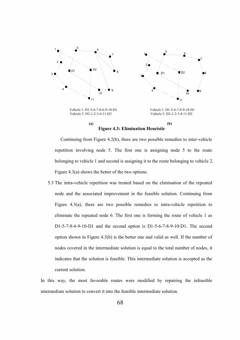
68

Vehicle 1: D1-5-6-7-8-6-9-10-D1 Vehicle 1: D1-5-6-7-8-9-10-D1

Vehicle 2: D2-1-2-3-4-11-D2 Vehicle 2: D2-1-2-3-4-11-D2

(a) (b)

Figure 4.3: Elimination Heuristic

Continuing from Figure 4.2(b), there are two possible remedies to inter-vehicle

repetition involving node 5. The first one is assigning node 5 to the route

belonging to vehicle 1 and second is assigning it to the route belonging to vehicle 2.

Figure 4.3(a) shows the better of the two options.

5.3 The intra-vehicle repetition was treated based on the elimination of the repeated

node and the associated improvement in the feasible solution. Continuing from

Figure 4.3(a), there are two possible remedies to intra-vehicle repetition to

eliminate the repeated node 6. The first one is forming the route of vehicle 1 as

D1-5-7-8-6-9-10-D1 and the second option is D1-5-6-7-8-9-10-D1. The second

option shown in Figure 4.3(b) is the better one and valid as well. If the number of

nodes covered in the intermediate solution is equal to the total number of nodes, it

indicates that the solution is feasible. This intermediate solution is accepted as the

current solution.

In this way, the most favorable routes were modified by repairing the infeasible

intermediate solution to convert it into the feasible intermediate solution.

-15

-10

-5

0

5

10

15

20

3

11

2

8D1

10

1

7

D2

4

56

9

-15

-10

-5

0

5

10

15

20

3

11

2

8D1

10

1

7

D2

4

56

9

69

4.3.4 �eighboring Approach for Updating the Sample Space

The standard procedure of updating the sample space and further sample in the

neighborhood of the most favorable strategy is explained in Step 7 of Section 3.4. It was

applied in the MDMTSP solution procedure only when the feasible solution was achieved.

The feasibility here refers to the solution having all the nodes selected with no repetition

and at least one node is selected by each vehicle. The corresponding heuristic techniques

are discussed in Section 4.3.3.

Instead of using the interval factor explained in Step 7 of Section 3.4, neighboring radii

were used to update the sample space in the solution procedure of MDMTSP. For the first

few iterations, sampling was carried out in the neighborhood of the nodes of a route by

considering very large neighboring radii covering all the nodes. This facilitates every

vehicle to select any available node and helps the algorithm to have an expanded search.

The neighboring radii were reduced progressively only when there was no change in the

solution for a predefined number of iterations. It is important to mention here that an

identical neighboring radius was applied to every node of a route corresponding to the

particular vehicle. Moreover, the nodes covered in that neighboring zone were eligible to

be selected by the vehicle for further iterations. An example with arbitrary neighboring

radius at some arbitrary iteration is shown in Figure 4.4. The circles around the nodes

belonging to vehicle 1 represent the neighboring zones. The nodes (5, 6, 7, 8, 9, 10 and 11)

in these zones are available to be sampled randomly for vehicle 1 for the next iteration.

70

Vehicle 1: D1-5-6-7-8-9-10-D1

Vehicle 2: D2-1-2-3-4-11-D2

Figure 4.4: �eighboring Approach

The procedure from Section 4.3.1 to 4.3.4 was repeated until there is no change in the

final solution or for a predefined number of iterations i.e. until convergence. On

convergence, the node swapping heuristic technique was applied. This is discussed in the

next section.

4.3.5 �ode Swapping Heuristic

The heuristic of swapping the set of arcs is one of the techniques used in the multi-

depot case in [154] and represented as inter-depot mutation by exchanging a set of arcs. In

the current work presented here, an approach similar to that in [154] but swapping the

entire set of nodes was implemented when there was no change in the current solution for

a predefined number of iterations. The entire sets of nodes belonging to two depots were

exchanged and the improved solution was accepted. This heuristic proved to be very

useful for the PC algorithm solving the two cases of the MDMTSP presented in the

following sections. This heuristic also helped in jumping out of local optima. Continuing

-15

-10

-5

0

5

10

15

20

3

11

2

8D1

10

1

7

D2

4

56

9

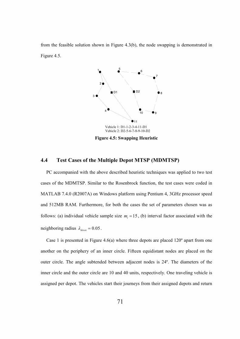
71

from the feasible solution shown in Figure 4.3(b), the node swapping is demonstrated in

Figure 4.5.

Vehicle 1: D1-1-2-3-4-11-D1

Vehicle 2: D2-5-6-7-8-9-10-D2

Figure 4.5: Swapping Heuristic

4.4 Test Cases of the Multiple Depot MTSP (MDMTSP)

PC accompanied with the above described heuristic techniques was applied to two test

cases of the MDMTSP. Similar to the Rosenbrock function, the test cases were coded in

MATLAB 7.4.0 (R2007A) on Windows platform using Pentium 4, 3GHz processor speed

and 512MB RAM. Furthermore, for both the cases the set of parameters chosen was as

follows: (a) individual vehicle sample size 15im = , (b) interval factor associated with the

neighboring radius 0.05downλ = .

Case 1 is presented in Figure 4.6(a) where three depots are placed 120º apart from one

another on the periphery of an inner circle. Fifteen equidistant nodes are placed on the

outer circle. The angle subtended between adjacent nodes is 24º. The diameters of the

inner circle and the outer circle are 10 and 40 units, respectively. One traveling vehicle is

assigned per depot. The vehicles start their journeys from their assigned depots and return

3

11

2

8D1

10

1

7

D2

4

56

9

72

to their corresponding depots. According to the geometry of the problem and also

assuming that the problem is symmetric (i.e. the cost of traveling between any two nodes

is the same in both directions), the true optimum traveling cost is attained when vehicle 1

at depot 1 traveled the route D1-3-4-5-6-7-D1, vehicle 2 at depot 2 traveled the route D2-

8-9-10-11-12-D2, and vehicle 3 at depot 3 traveled the route D3-13-14-15-1-2-D3. The

true optimum solution was achieved by the PC approach and is plotted in Figure 4.6(b).

(a) Case 1 (b) Solution to Case 1

Figure 4.6: Test Case 1

According to the coordinates of the nodes and the depots, the optimum cost of

traveling each of these routes is 134.7870 units. Hence, the optimum total traveling cost is

404.3610 units. A total of 50 runs were conducted for Case 1 and the true optimum was

reached in every run. The time to reach the optimum varied between 0.35 minutes and

3.83 minutes with an average time of 2.09 minutes. The convergence plot of one of the

runs is shown in Figure 4.7 in which the solution at iteration 21 was accepted as the final


-40 -30 -20 -10 0 10 20 30 40

-40

-30

-20

-10

0

10

20

30

40

2

13

15

D1

1

34

5

6

7

8

9

10

1112

14

D2

D3

-40 -30 -20 -10 0 10 20 30 40

-40

-30

-20

-10

0

10

20

30

40

2

13

15

D1

1

34

5

6

7

8

9

10

1112

14

D2

D3

73

Figure 4.7: Convergence Plot for Test Case 1

Case 2 is presented in Figure 4.8(a) where three depots are placed 120º apart from one

another on the periphery of an inner circle. Fifteen nodes are placed on the outer circle.

These nodes are arranged in three clusters. In every cluster, the nodes are intentionally

placed at uneven angles apart. The diameters of the inner circle and the outer circle are 5

and 10 units, respectively. Similar to Case 1, one vehicle is assigned per depot. The

vehicles start their journeys from their assigned depots and return to their corresponding

depots. According to the geometry of the problem and also assuming that the problem is

symmetric, the optimum traveling cost is attained when vehicle 1 at depot 1 traveled the

route D1-6-7-8-9-10-D1, vehicle 2 at depot 2 traveled the route D2-11-12-13-14-15-D2,

and vehicle 3 at depot 3 traveled the route D3-1-2-3-4-5-D3. The true optimum solution

was achieved by the PC approach and is plotted in Figure 4.8(b).

400

450

500

550

600

650

1 3 5 7 9 11 13 15 17 19 21 23 25 27

Total Traveling Cost

Iterations

74

(a) Case 2 (b) Solution to Case 2

Figure 4.8: Test Case 2

According to the coordinates of the nodes and the depots, the optimum cost of

traveling each of these routes is 20.4264 units. Hence, the optimum total traveling cost is

61.2792 units. For case 2, more than 50 runs were conducted and the true optimum was

achieved in every run. The time to reach the optimum varied between 0.76 minutes and

3.10 minutes with an average time of 1.27 minutes. The convergence plot for one of the

runs is shown in Figure 4.9 in which the solution at iteration 33 was accepted as the final


Figure 4.9: Convergence Plot for Test Case 2

-10 -5 0 5 10

10

14

1

3

7

12

13

1

2

3

4

5

6

8

9

11

15

D1

D2

D3

-10 -5 0 5 10

10

14

1

3

7

12

13

1

2

3

4

5

6

8

9

11

15

D1

D2

D3

60

110

160

210

260

1 3 5 7 9 11 13 15 17 19 21 23 25 27 29 31 33 35 37


Iterations

75

4.5 Test Cases of the Single Depot MTSP (SDMTSP) with Randomly

Located �odes

Using the same procedure as the above test cases of the MDMTSP, over 30 cases of

the Single Depot MTSP (SDMTSP) with 3 vehicles and 15 nodes were solved. In all the

cases, the single depot and the 15 nodes were randomly located in an area of 100 × 100

units. Two sample cases are shown in Figure 4.10(a) and 4.11(a) and the corresponding

convergence plots in 4.10(b) and 4.11(b). In the first sample, the solution at iteration 19

and for the second sample case, the solution at iteration 33 was accepted as the final ones as

there was no change in the respective solutions for a considerable number of iterations. In all the

cases with randomly located nodes, the approximate convergence time was found to vary

between 1 minute and 6 minutes with an average time of 3.34 minutes.

76

(a)

(b)

Figure 4.10: Randomly Located �odes (Sample Case 1)

1

2

34

5

6

7

8

9

1

2

34

5

6

7

8

9

1

2

3

4

5

6

7

8 9

10

1112

1314

15

D

525

575

625

675

725

775

825

1 3 5 7 9 11 13 15 17 19 21 23 25 27 29 31


Iterations

77

(a)

(b)

Figure 4.11: Randomly Located �odes (Sample Case 2)

4.6 Comparison and Discussion

The above solution to the MDMTSP and SDMTSP using PC indicates that it can

successfully be used to solve the combinatorial optimization problems. As shown in Table

4.2, the results are compared with those of some other methods solving the problem with

30 40 50 60 70 80 90 100

1

2

3

4

5

6

7

8

9

10

11

12

13

14

15

1

2

3

4

5

6

7

8

9

10

11

12

13

14

15

1

2

3

4

5

6

7 8

9

10

11

12

13

14

15

D

400

450

500

550

600

650

700

750

800

1 3 5 7 9 11 13 15 17 19 21 23 25 27 29 31 33 35 37 39 41 43 45


Iterations

78

sizes close to the specially developed test cases solved here. It is worth mentioning that

the technique of converting the MTSP into the standard TSP using Miliotis reverse

algorithm [154], cutting plane algorithm [133], elastic net approach [142] as well as

Branch and Bound techniques such as ‘branch on an arc’ and ‘branch on a route’ with

different lower bounds (LB0, LB2, etc.) in [132] did not produce the optimum solution in

every run. It therefore requires the algorithms to be run for a number of trials and then

accepting the average from among the trials as the solution. On the other hand, every run

of the PC converged to the actual optimal solution for the MDMTSP in quite reasonable

CPU time. In case of the SDMTSP, the percentage deviation of total traveling cost from

the average solution over 30 runs of PC was recorded to be 2.94%. Furthermore, the CPU

time varied within a very small range. The time variation exists because of the

probabilistic nature of PC algorithm and random initial sampling of the routes affecting

every subsequent step. As per the literature review in Section 4.2.3, the popular

optimization techniques are computationally time consuming and expensive. It is also

worth to mention that the above insertion, elimination and swapping heuristics could be

easily accommodated into PC.

79

Table 4.2: Performance Comparison of Various Algorithms solving the MTSP

Method �odes Vehicles Avg. CPU Time

(Minutes)

% Deviation

MTSP to std.

TSP [154]

20

20

20

2

3

4

2.05

2.47

2.95

--

Cutting Plane

[133]

20

20

20

2

3

4

1.71

1.50

1.44

--

--

Elastic Net+ [142] 22

22

22

2

3

4

12.03

13.10

12.73

28.71

74.18

33.33

Branch on an Arc

with LB0 [132]

15 3 0.56 --

Branch on an Arc

with LB2 [132]

15

20

3

4

1.01

2.32

--

Branch on a

Route with LB0

[132]

15 3 0.44 --

PC

(MDMTSP)

15 (Case 1)

15 (Case 2)

3

3

2.09

1.27

0.00

0.00

PC

(SDMTSP)

15

3

3.34

2.94

+: unable to reach the optimum

Besides the advantages of PC, some weaknesses associated with the above solution

procedure solving the MTSP were also identified. As an effort to deal with constraints,

various heuristic techniques were incorporated which served as repair techniques to push

the solution into feasibility. This may not be an elegant option since they cannot be used

for handling generic constraints. If complexity of the problem and related constraints

increase, the repair work may become more tedious and may add further computational

load. In addition, the number of function evaluations can become very large because of its

dependence on the number of strategies in every agent’s strategy sets. Both of these

disadvantages may limit its use to smaller size problems with fewer constraints. In order to

avoid this limitation and develop a more generic constraint handling technique, a penalty

80

function approach is incorporated in to PC algorithm. This is described in the following

chapter.

81

CHAPTER 5


There are a number of traditional constraint handling methods available, such as

gradient projection method, reduced gradient method, Lagrange multiplier method,

aggregate constraint method, feasible direction based method, penalty based method, etc

[96, 97]. The penalty based methods can be referred to as generalized constraint handling

methods because of their simplicity, ability to handle nonlinear constraints and can be

used with most of the unconstrained optimization methods [96, 97]. They basically

transform a constrained optimization problem into an unconstrained optimization problem.

A constrained PC algorithm is proposed in this chapter by incorporating the penalty

function approach and associated modifications to the unconstrained PC approach

described in Chapter 3. The constrained PC approach was validated by successfully

solving three constrained test problems [6]. The resulting constrained PC algorithm

flowchart is presented in Figure 5.1.

5.1 Penalty Function Approach

Consider a general constrained problem (in the minimization sense) as follows:

Minimize G (5.1)

Subject to 0 , 1, 2,...,

0, 1, 2,...,

j

j

g j s

h j t

≤ =

= =

For each of its combined strategy set [ ]r

iY , each agent i computes the corresponding

system objective ( )[ ]r

iG Y [1, 2], i.e. each agent i computes im values of the system

82

objective ( )[ ]r

iG Y . In addition, each agent i computes im vectors of the corresponding

constraints ( )[ ]r

iC Y as follows:

( ) ( ) ( ) ( ) ( ) ( ) ( )

( ) ( ) ( ) ( ) ( ) ( ) ( )

( ) ( ) ( ) ( ) ( ) ( ) ( )

[1] [1] [1] [1] [1] [1] [1]

1 2 1 2

[ ] [ ] [ ] [ ] [ ] [ ] [ ]

1 2 1 2

[ ] [ ] [ ] [ ] [ ] [ ] [ ]

1 2 1 2

... ...

... ...

... ...i i i i i i i

i i i s i i i t i

r r r r r r r

i i i s i i i t i

m m m m m m m

i i i s i i i t i

g g g h h h

g g g h h h

g g g h h h

=

=

=

C Y Y Y Y Y Y Y

C Y Y Y Y Y Y Y

C Y Y Y Y Y Y Y

⋮

⋮

(5.2)

where s is the number of inequality constraints and t is the number of equality

constraints.

In order to incorporate the constraints into the problem, each agent i forms the

pseudo-objective function as follows [96, 97]:

[ ]( ) ( ) ( ) ( )2 2

[ ] [ ] [ ]

1 1

s tr r r r

i i j i j i

j j

G g hφ θ +

= =

= + + ∑ ∑Y Y Y Y (5.3)

where ( ) ( )( )[ ] [ ]max 0,r r

j i j ig g+ =Y Y and θ is the scalar penalty parameter.

The ultimate goal of every agent i is to identify its own strategy value which

contributes the most towards the minimization of the sum of these system objective values,

i.e. [ ]

1

( )im

r

i

r

φ=∑ Y , referred to as the collection of pseudo-system objectives.

In addition to the parameters listed in the unconstrained PC algorithm in Section 3.4,

four more parameters are required in the constrained algorithm, namely the number of test

iterations testn which decides the iteration number from which the convergence condition

needs to be checked, the scalar penalty parameter θ , the associated update factor θα for

83

the parameter θ and a constraint violation tolerance µ . Similar to the other parameters,

the values of these parameters are chosen based on the preliminary trials of the algorithm.

Furthermore, at the beginning of the algorithm, the tolerance µ is initialized to a very

large prescribed value. The value of µ is tightened iteratively as the algorithm progresses.

The system objective [ ]( )fav


Y are accepted if and only if

the largest absolute component from the constraint vector [ ]( )fav

C Y referred to as maxC is

not worse than the constraint violation tolerance µ , i.e., maxC µ≤ , and the value of µ is

updated to maxC , i.e.,

maxCµ = . In this way the algorithm progresses by iteratively

tightening the constraint violation.

The detailed illustration of the above mentioned modifications to the unconstrained PC

algorithm (discussed in Chapter 3) corresponding to the decision of acceptance/rejection

of the solution, the updating of the parameters are represented in windows A and B

respectively, of the constrained PC algorithm flowchart shown in Figure 5.1.

84

Figure 5.1: Constrained PC Algorithm Flowchart (Penalty Function Approach)

START

Initialize n , initialT T= , Tα , θα , penalty parameter θ , constraint violation tolerance

µ . For every agent i set up strategy set iX with im strategies.

Form combined strategy set [ ]riY for every strategy r of agent i , compute [ ]( )r

iG Y and

constraints [ ]( )r

iC Y , pseudo-objective function [ ]( )r

iφ Y and corresponding collection of

pseudo-system objectives [ ]

1

( )im

r

i

r

φ=∑ Y

Set probabilities ( )iq X as variables and assign uniform values, i.e. [ ]: ( ) 1/

riir q X m∀ =

and compute expected collection of pseudo-system objectives ( )[ ]

1

( )im

r

i

r

E φ=∑ Y

Form the modified Homotopy function ( )( )J ,i i

q TX

Minimize the Homotopy function using second order optimization technique such as

Nearest Newton Method

Obtain the probability distribution ( )iq X for every agent i clearly distinguishing every

corresponding strategy’s contribution and identifying every agent’s favourable strategy [ ]fav

iX

Compute the objective function [ ]( )

favG Y , constraints [ ]

( )fav

C Y and maximum constraint

value maxC

maxC ≤ µ

Accept current objective function [ ]

( )fav

G Y and related [ ]favY

N

Discard current [ ]( )

favG Y and retain

previous [ ]( )

favG Y and related [ ]fav

Y

Y

maxCµ =

B

STOP

Accept [ ]( )

favG Y as

[ ]( )fav finalG Y along with

related [ ]favY

Convergence?

Y N

A For each agent i , update

the sampling interval iΨ

and form corresponding

updated strategy set iX

1n n= + , TT T Tα= − ,

Update penalty Parameter

θθ θ α θ= +

85

5.2 Solutions to Constrained Test Problems

The constrained PC approach was successfully tested for solving three problems with

equality and inequality constraints. These problems have already been well studied in the

literature and used to compare the performance of various optimization algorithms. The

various associated constraint handling techniques are discussed below in brief.

Some of the approaches [155-159] focused on overcoming the limitations of the classic

penalty approach. A self adaptive penalty approach [155] and dynamic penalty scheme

[157] produced premature convergence and similar to stratum approach [158] were quite

sensitive to the additional set of parameters. A stochastic bubble sort algorithm in [156]

attempted the direct and explicit balance between the objective function and the penalty

function. Although a variety of constrained problems could be solved, it was sensitive to

the associated probability parameter and needed several preliminary trials. The approach

of penalty parameter was avoided using a feasibility-based rule in [159]. It required an

additional fitness function and failed to produce optimum solution in every run. In

addition, the quality of the solution was governed by the population in hand. The need of

additional fitness function was avoided in Hybrid PSO [160] by incorporating the

feasibility-based rules [159] into PSO.

The GEnetic algorithm for Numerical Optimization of COnstrained Problems

(GENOCOP) specifically for linear constraints [161, 162], the PSO [163] and the

Homomorphous Mapping [164] needed initial feasible solutions along with the problem

dependent parameters to be set. Furthermore, for some of the problems, it was almost

impossible to generate initial feasible solutions, which might need some additional

techniques. The lack of diversity of the population was noticed in the cultural algorithm

86

[165] and Cultural Differential Evolution (CDE) [166] which divide the search space into

feasible, semi-feasible and infeasible regions.

An interactive approach of constraint correction algorithm [96] needed an additional

constraint and several preliminary trials. The gradient repair method [167] was embedded

into PSO [168] and its performance was governed by the number of solutions undergoing

repair [169].

The multi-objective approach in Filter SA (FSA) [170] required numerous problem

dependent parameters to be tuned along with the associated preliminary trials. Inspired

from [170], GA was applied to find the non-dominated solution vector in [171]. The

multi-criteria approach problem in [172-174] could not solve the fundamental problem of

balancing the objective function and the constraint violations. The results of the two multi-

objective approaches in [175] highlighted the necessity of an additional search bias

technique to locate the feasible solutions.

In this current work, the constrained PC algorithm was coded in MATLAB 7.4.0

(R2007A) and the simulations were run on a Windows platform using a Pentium 4, 3GHz

processor speed and 512MB memory capacity. The results and the comparison with other

algorithms are discussed below.

5.2.1 Test Problem 1

This is a tension/compression spring design problem described in [96, 155, 160, 165,

171]. It has the aim of minimizing the weight ( )f X of a tension/compression spring (as

shown in Figure 5.2) subject to constraints on minimum deflection, shear stress, surge

frequency, limits on outside diameter and on design variables. The design variables are the

87

mean coil diameter, the wire diameter 1x and the number of active coils

3x . This problem

is categorized as a quadratic problem with three variables, six boundary conditions, one

linear inequality and three nonlinear inequality constraints.

Figure 5.2: Tension/Compression Spring

The mathematical formulation of this problem can be described as follows:

( ) ( )

( )

( ) ( )

( )

( )

2

3 2 1

3

2 31 4

1

2

2 1 22 23 4

12 1 1

13 2

2 3

1 24

Minimize 2

Subject to 1 071785

4 11 0

510812566

140.451 0

1 01.5

f x x x

x xg

x

x x xg

xx x x

xg

x x

x xg

= +

= − ≤

−= + − ≤

−

= − ≤

+= − ≤

X

X

X

X

X

where 1 2 30.05 2, 0.25 1.3, 2 15x x x≤ ≤ ≤ ≤ ≤ ≤

This problem was solved in [96, 155, 160, 165, 171]. The best solutions obtained by

these approaches along with those by the PC approach are listed in Table 5.1. The PC

solution to the problem produced competent results at low computational cost

(computational costs of the other approaches were not available). The best, mean and

worst function values found from ten runs were 0.01350, 0.02607, 0.05270, respectively.

Furthermore, the average CPU time in seconds and average number of function

2x

1x

PP

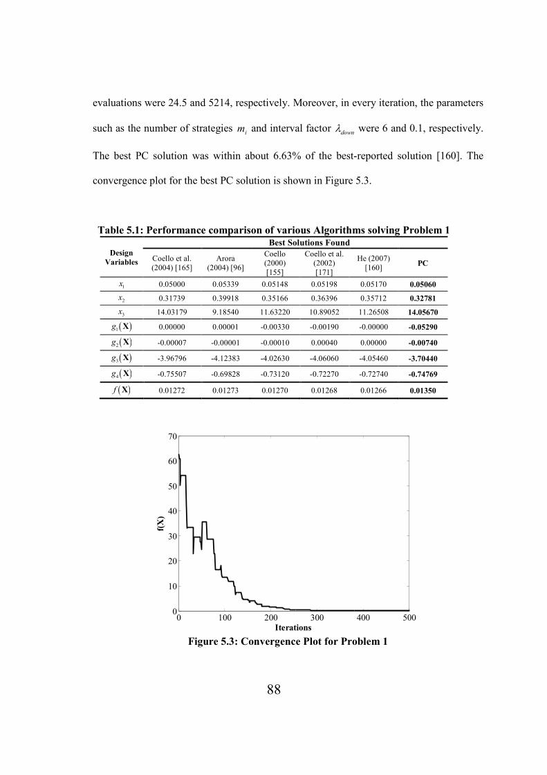
88

evaluations were 24.5 and 5214, respectively. Moreover, in every iteration, the parameters

such as the number of strategies im and interval factor

downλ were 6 and 0.1, respectively.

The best PC solution was within about 6.63% of the best-reported solution [160]. The

convergence plot for the best PC solution is shown in Figure 5.3.

Table 5.1: Performance comparison of various Algorithms solving Problem 1

Design

Variables

Best Solutions Found

Coello et al.

(2004) [165]

Arora

(2004) [96]

Coello

(2000)

[155]

Coello et al.

(2002)

[171]

He (2007)

[160] PC

1x 0.05000 0.05339 0.05148 0.05198 0.05170 0.05060

2x 0.31739 0.39918 0.35166 0.36396 0.35712 0.32781

3x 14.03179 9.18540 11.63220 10.89052 11.26508 14.05670

( )1g X 0.00000 0.00001 -0.00330 -0.00190 -0.00000 -0.05290

( )2g X -0.00007 -0.00001 -0.00010 0.00040 0.00000 -0.00740

( )3g X -3.96796 -4.12383 -4.02630 -4.06060 -4.05460 -3.70440

( )4g X -0.75507 -0.69828 -0.73120 -0.72270 -0.72740 -0.74769

( )f X 0.01272 0.01273 0.01270 0.01268 0.01266 0.01350

Figure 5.3: Convergence Plot for Problem 1

0 100 200 300 400 5000

10

20

30

40

50

60

70

Iterations

f(X

)

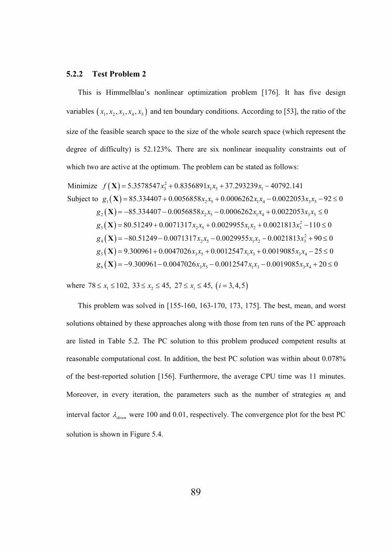
89


This is Himmelblau’s nonlinear optimization problem [176]. It has five design

variables ( )1 2 3 4 5, , , ,x x x x x and ten boundary conditions. According to [53], the ratio of the

size of the feasible search space to the size of the whole search space (which represent the

degree of difficulty) is 52.123%. There are six nonlinear inequality constraints out of

which two are active at the optimum. The problem can be stated as follows:

( )( )

( )( )

2

3 1 5 1

1 2 5 1 4 3 5

2 2 5 1 4 3 5

3

Minimize 5.3578547 0.8356891 37.293239 40792.141

Subject to 85.334407 0.0056858 0.0006262 0.0022053 92 0

85.334407 0.0056858 0.0006262 0.0022053 0

80.51249 0

f x x x x

g x x x x x x

g x x x x x x

g

= + + −

= + + − − ≤

= − − − + ≤

= +

X

X

X

X

( )( )( )

2

2 5 1 2 3

2

4 2 5 1 2 3

5 3 5 1 3 3 4

6 3 5

.0071317 0.0029955 0.0021813 110 0

80.51249 0.0071317 0.0029955 0.0021813 90 0

9.300961 0.0047026 0.0012547 0.0019085 25 0

9.300961 0.0047026 0.0012547

x x x x x

g x x x x x

g x x x x x x

g x x

+ + − ≤

= − − − − + ≤

= + + + − ≤

= − − −

X

X

X 1 3 3 40.0019085 20 0x x x x− + ≤

where ( )1 278 102, 33 45, 27 45, 3, 4,5ix x x i≤ ≤ ≤ ≤ ≤ ≤ =

This problem was solved in [155-160, 163-170, 173, 175]. The best, mean, and worst

solutions obtained by these approaches along with those from ten runs of the PC approach

are listed in Table 5.2. The PC solution to this problem produced competent results at

reasonable computational cost. In addition, the best PC solution was within about 0.078%

of the best-reported solution [156]. Furthermore, the average CPU time was 11 minutes.

Moreover, in every iteration, the parameters such as the number of strategies im and

interval factor downλ were 100 and 0.01, respectively. The convergence plot for the best PC

solution is shown in Figure 5.4.

90

Table 5.2: Performance comparison of various Algorithms solving Problem 2 Algorithm Best Mean Worst Std Dev Average

Function

Evaluations

Coello et al. (2004)

[165]

-30665.5000 -30662.5000 -30636.2000 9.3

Becerra et. al. (2006)

[166]

-30665.5386 -30665.5386 -30665.5386 0.00000

Koziel et al. (1999)

[164]

-30664.0000 -30655.0000 -30645.0000 -- 1400000

Hedar et al. (2006)

[170]

-30665.5380 -30665.4665 -30664.6880 0.173218 86154

Coello (2000) [155] -31020.8590 -30984.2400 -30792.4070 73.633 --

Chootinan et al.

(2006) [167]

-30665.5386 -30665.3538 -30665.5386 0.000000 26981

Runarsson et al.

(2005) [175]

-30665.5386 -30665.3539 -30665.5386 0.000000 66400

Runarsson et al.

(2000) [156]

-30665.5390 -30665.5390 -30665.5390 1.1E-11 350000

Zahara et al. (2008)

[168]

-30665.5386 -30665.35386 -30665.5386 0.000000 19658

Deb (2000) [159] -30665.5370 -- 29846.6540 --

Farmani et al. (2003)

[157]

-30665.5000 -30665.2000 -30663.3000 4.85E-01 --

Hu et al. (2002) [163] 30665.5000 30665.5000 30665.5000 -- --

Dong et al. (2005)

[169]

-30664.7000 -30662.8000 -30656.1000 -- --

Ray et al. (2001)

[173]

-30651.6620 -30647.1050 -30619.0470 -- 35408

He et al. (2007) [160] -30665.5390 -30665.5390 -30665.5390 1.7E-06

Homaifar et al.

(1994) [158]

-30373.9500 -- -30175.8040 -- --

PC -30641.5702 -30635.4157 -30626.7492 7.5455 2780449


0 500 1000 1500 2000 2500 3000 3500-3.1

-3

-2.9

-2.8

-2.7

-2.6

-2.5

-2.4

-2.3

-2.2x 10

4

Iterations

f(X

)

91


This problem is categorized as logarithmic nonlinear with ten variables, ten boundary

conditions and three linear equality constraints. The problem can be stated as follows:

( )

( )( )( )

10

1 1 2 10

1 1 2 3 6 10

2 4 5 6 7

3 3 7 8 9 10

Minimize ln...

Subject to 2 2 2 0

2 1 0

2 1 0

0.000001, 1,2,...,10

j

j j

j

i

xf x c

x x x

h x x x x x

h x x x x

h x x x x x

x i

=

= + + + + = + + + + − =

= + + + − =

= + + + + − =

≥ =

∑X

X

X

X

where

1 2 3 4 5

6 7 8 9 10

6.089 17.164 34.054 5.914 24.721

14.986 24.100 10.708 26.662 22.179

c c c c c

c c c c c

= − = − = − = − = −

= − = − = − = − = −

This problem is a modified version of the chemical equilibrium problem in complex

mixtures originally presented in [177]. The modified problem was solved in [162, 178].

The best solutions obtained by these approaches along with those by the PC approach are

listed in Table 5.3. The PC solution to this problem produced competent results but at high

computational cost (computational costs of the other approaches were not available). The

best, mean and worst function values found from ten runs were -46.7080572120, -

45.6522267370, -44.4459333503, respectively, with standard deviation 0.7893.

Furthermore, the average CPU time for PC solution was 21.60 min. Moreover, in every

iteration, the parameters such as the number of strategies im and interval factor

downλ were

6 and 0.1, respectively. The best PC solution was within about 2.20% of the best-reported

solution [162]. The convergence plot for the best PC solution is shown in Figure 5.5.

92

Table 5.3: Performance Comparison of Various Algorithms Solving Problem 3 Design Best Solutions Found

Variables Hock et al. (1981)

[178]

Michalewicz (1997)

[162]

PC

1x 0.01773548 0.04034785 0.0308207485

2x 0.08200180 0.15386976 0.2084261218

3x 0.88256460 0.77497089 0.6708869580

4x 0.0007233256 0.00167479 0.0371668767

5x 0.4907851 0.48468539 0.3510055351

6x 0.0004335469 0.00068965 0.1302810195

7x 0.01727298 0.02826479 0.1214712339

8x 0.007765639 0.01849179 0.0343070642

9x 0.01984929 0.03849563 0.0486302636

10x 0.05269826 0.10128126 0.0486302636

( )1h X 8.6900E-08 6.0000E-08 -0.0089160590

( )2h X 0.0141 1.0000E-08 -0.0090697995

( )3h X 5.9000E-08 -1.0000E-08 -0.0047181958

( )f X -47.707579 -47.760765 -46.7080572120

Average

Function

Evaluations

-- -- 389546


0 200 400 600 800 1000-7

-6

-5

-4

-3

-2

-1

0x 10

4

Iterations

f(X

)

8800 9000

93

5.3 Discussion

The above solutions using PC indicated that it can successfully be used to solve a

variety of constrained optimization problems. The results also demonstrated its

competitiveness with those of some other methods. Furthermore, it was evident from the

results that the approach is sufficiently robust and produced consistent results in every run.

It implies that the rational behavior of the agents could be successfully formulated and

demonstrated.

The worthy features of the above constrained PC approach are discussed here by

comparing with some other methods. Approaches such as PSO [163], Homomorphous

Mapping [164], GENOCOP [162] require initial feasible solution, whereas the constrained

PC approach proposed here can solve the problems starting from randomly generated and

completely infeasible solutions. The approach presented here can handle both equality as

well as inequality constraints, whereas the approach of concurrent co-evolution in [155] is

applicable only to inequality constraints with further additional computations involved.

The method of GENOCOP [161, 162] is suitable only for the linear constraints while the

proposed approach can handle both linear and nonlinear constraints.

Besides the advantages of the present approach, some limitations were also identified.

The rate of convergence and the quality of the solution was dependent on the parameters

such as the number of strategies im in every agent’s strategy set

iX and the interval factor

downλ . Some preliminary trials were also necessary for fine-tuning these parameters. Based

on the results and the trials performed, it was also noticed that the PC method is quite

efficient in searching the feasible region and the local minima (in the vicinity of the true

94

optimum) but demonstrates weak local search ability which may be necessary to reach the

true optimum.

The next chapter discusses two variations of the Feasibility-based Rule as an effort to

make PC a more versatile optimization approach.

95

CHAPTER 6


This chapter demonstrates further efforts to develop a generic constraint handling

technique for PC in order to make it a more versatile optimization algorithm. Two

variations of the Feasibility-based Rule referred to as Feasibility-based Rule I and II

originally proposed in [159] and further implemented in [160, 179-183] were incorporated

into the unconstrained PC approach from Chapter 3.

Consider a general constrained problem (in the minimization sense) as follows:

Minimize G (6.1)

Subject to 0 , 1, 2,...,

0, 1, 2,...,

j

j

g j s

h j w

≤ =

= =

According to [172-174], the equality constraint 0jh = can be transformed into a pair

of inequality constraints using a tolerance value δ as follows:

0 1, 2,...,0

0

s j j

j

s w j j

g h j wh

g h

δ

δ+

+ +

= − ≤ == ⇒

= − − ≤ (6.2)

Thus, w equality constraints are replaced by 2w inequality constraints with the total

number of constraints given by 2t s w= + . Then a generalized representation of the

problem in equation (6.1) can be stated as follows:

Minimize G (6.3)

Subject to 0 , 1, 2,...,jg j t≤ =

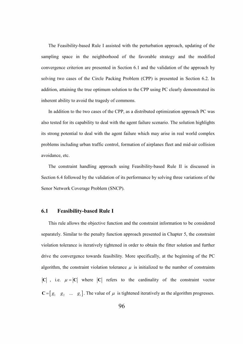
96

The Feasibility-based Rule I assisted with the perturbation approach, updating of the

sampling space in the neighborhood of the favorable strategy and the modified

convergence criterion are presented in Section 6.1 and the validation of the approach by

solving two cases of the Circle Packing Problem (CPP) is presented in Section 6.2. In

addition, attaining the true optimum solution to the CPP using PC clearly demonstrated its

inherent ability to avoid the tragedy of commons.

In addition to the two cases of the CPP, as a distributed optimization approach PC was

also tested for its capability to deal with the agent failure scenario. The solution highlights

its strong potential to deal with the agent failure which may arise in real world complex

problems including urban traffic control, formation of airplanes fleet and mid-air collision

avoidance, etc.

The constraint handling approach using Feasibility-based Rule II is discussed in

Section 6.4 followed by the validation of its performance by solving three variations of the

Senor Network Coverage Problem (SNCP).

6.1 Feasibility-based Rule I

This rule allows the objective function and the constraint information to be considered

separately. Similar to the penalty function approach presented in Chapter 5, the constraint

violation tolerance is iteratively tightened in order to obtain the fitter solution and further

drive the convergence towards feasibility. More specifically, at the beginning of the PC

algorithm, the constraint violation tolerance µ is initialized to the number of constraints

C , i.e. µ = C where C refers to the cardinality of the constraint vector

[ ]1 2 ... tg g g=C . The value of µ is tightened iteratively as the algorithm progresses.

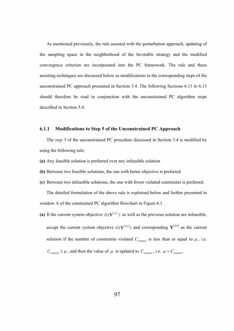
97

As mentioned previously, the rule assisted with the perturbation approach, updating of

the sampling space in the neighborhood of the favorable strategy and the modified

convergence criterion are incorporated into the PC framework. The rule and these

assisting techniques are discussed below as modifications to the corresponding steps of the

unconstrained PC approach presented in Section 3.4. The following Sections 6.11 to 6.13

should therefore be read in conjunction with the unconstrained PC algorithm steps

described in Section 3.4.

6.1.1 Modifications to Step 5 of the Unconstrained PC Approach

The step 5 of the unconstrained PC procedure discussed in Section 3.4 is modified by

using the following rule:

(a) Any feasible solution is preferred over any infeasible solution

(b) Between two feasible solutions, the one with better objective is preferred

(c) Between two infeasible solutions, the one with fewer violated constraints is preferred.

The detailed formulation of the above rule is explained below and further presented in

window A of the constrained PC algorithm flowchart in Figure 6.1.

(a) If the current system objective [ ]( )fav

G Y as well as the previous solution are infeasible,

accept the current system objective [ ]( )fav


Y as the current

solution if the number of constraints violated violatedC is less than or equal to µ , i.e.

violatedC µ≤ , and then the value of µ is updated to violatedC , i.e.

violatedCµ = .

98

(b) If the current system objective [ ]( )fav

G Y is feasible, and the previous solution is

infeasible, accept the current system objective [ ]( )fav


Y as

the current solution, and then the value of µ is updated to 0, i.e. 0violatedCµ = = .

(c) If the current system objective [ ]( )fav

G Y is feasible, i.e. 0violatedC = and is not worse

than the previous feasible solution, accept the current system objective [ ]( )fav

G Y and


Y as the current solution.

(d) If all the above conditions (a) to (c) are not met, then discard current system objective

[ ]( )fav


Y , and retain the previous iteration solution.


As mentioned previously, similar to [159, 160, 179-183] where additional techniques

were implemented to avoid premature convergence, a perturbation approach was also

incorporated. It perturbs the individual agent’s favorable strategy set based on its

reciprocal and associated predefined interval. The solution is accepted if the feasibility is

maintained. In this way, the algorithm continues until convergence by selecting the

samples from the neighborhood of the recent favorable strategies. Unlike the

unconstrained PC approach described in Chapter 3 and the Penalty Function Approach

discussed in Chapter 5 where the sampling space was reduced to the neighborhood of the

favorable strategy, in this case the sampling space in the neighborhood of the favorable

strategy is reduced or expanded according to the improvement in the system objective for

a predefined number of iterations. The detailed formulation of the updating of the

99

sampling space and the perturbation approach is explained below and further presented in

window B of the constrained PC algorithm flowchart in Figure 6.1.

On completion of the pre-specified testn iterations of the PC algorithm, the following

conditions are checked in every further iteration.

(a) If [ ] [ ], ,( ) ( )testfav n fav n n

G G−≤Y Y , then every agent shrinks its sampling interval as follows:


i i down i i i down i iX Xλ λ Ψ ∈ − Ψ −Ψ + Ψ −Ψ , 0 1downλ< ≤

(6.4)

where downλ is referred to as the interval factor corresponding to the shrinking of

sample space.

(b) If [ ],( )

fav nG Y and [ ],

( )testfav n nG

−Y are feasible and

[ ] [ ], ,( ) ( )testfav n fav n n

G G ε−− ≤Y Y , the

system objective [ ],( )fav n

G Y can be referred to as a stable solution [ ],( )fav s

G Y or

possible local minimum.

In order to jump out of this possible local minimum, every agent i perturbs its current

favorable strategy [ ]fav

iX by a perturbation factor ifact corresponding to the reciprocal of

its favorable strategy [ ]fav

iX as follows:

[ ] [ ] [ ]( )fav fav fav

i i i iX X X fact= ± × (6.5)

where

( ) [ ]

( ) [ ]

1 1

2 2

1,

1,

lower upper

fav

i

i

lower upper

fav

i

randomvalue ifX

fact

random value ifX

σ σ γ

σ σ γ

∈ ≤

= ∈ >

100

and 1 1 2 2, , ,lower upper lower upperσ σ σ σ are randomly generated values between 0 and 1 i.e.,

1 1 2 20 1lower upper lower upperσ σ σ σ< < ≤ < < . The value of γ as well as ‘+’ or ‘-’ sign in equation

(6.5) are chosen based on the preliminary trials of the algorithm.

It gives a chance to every agent i to jump out of the local minima and may further

help to search for a better solution. The perturbed solution is accepted if and only if the

feasibility is maintained. Furthermore, every agent expands its sampling interval as

follows:

( ) ( ),lower upper lower upper upper lower

i i up i i i up i iλ λ Ψ ∈ Ψ − Ψ −Ψ Ψ + Ψ −Ψ , 0 1upλ< ≤

(6.6)

where upλ is referred to as the interval factor corresponding to the expansion of sample

space.

6.1.3 Modifications to Step 6 of the Unconstrained PC approach

The detailed formulation of the modified convergence criterion is explained below and

further presented in window C of the constrained PC algorithm flowchart in Figure 6.1.

The current stable system objective [ ],( )fav s

G Y and corresponding [ ],fav s

Y are accepted

as the final solution referred to as [ ],( )fav final

G Y and

[ ] [ ] [ ] [ ] [ ]{ }, , , , ,


! !X X X X−=Y , if and only if either of the

following conditions is satisfied.

(a) If temperature finalT T= or 0T → .

101

(b) If there is no significant change in the successive stable system objectives (i.e.

[ ] [ ], , 1( ) ( )

fav s fav sG G ε−− ≤Y Y ) for two successive implementations of the perturbation

approach.

102

Figure 6.1: Constrained PC Algorithm Flowchart (Feasibility-based Rule I)

START

For every agent set up a strategy set with im strategies, assign uniform probabilities to

every agent’s strategies, initialize n , T , testn , µ = C

Form im combined strategy sets associated with every agent

Form the Homotopy function for each agent

For each agent minimize the Homotopy function using BFGS method and obtain the

probability distribution for every agent identifying its favorable strategy

STOP

Compute the system objective function and associated constraints

Compute im objective functions and associated expected local objectives for each agent

A

B

current feasible system

objective ≤ previous

feasible system

objective?

Accept current

objective function

and related strategies

Y

Discard current and

retain previous

objective function with

related strategies

N Is the solution

feasible?

Y N number of constraints

satisfied ≥ previous

solution constraints?

Accept current

objective function


Discard current and

retain previous


related strategies

Y N

Y

testn n≥ N

Solution remains

unchanged for successive

testn iterations?

Expand the sampling

interval

Shrink the

sampling interval

Y

N

Solution is feasible and

remains unchanged for

successive testn iterations? Apply self-adaptive

perturbation

N

1n n= + ,

TT T Tα= − N

Y

Accept the system

objective as final solution

along with agents’

associated strategies

Convergence

?

Y

C

103

6.2 The Circle Packing Problem (CPP)

A generalized packing problem consists of determining how best to pack z objects

into a predefined bounded space that yields best utilization of space with no overlap of

object boundaries [184, 185]. The bounded space can also be referred to as a container.

The packing objects and container can be circular, rectangular or irregular. Although the

problem appears rather simple and in spite of its practical applications in production and

packing for the textile, apparel, naval, automobile, aerospace, food industries, etc. [32] the

CPP received considerable attention in the ‘pure’ mathematics literature but only limited

attention in the operations research literature [33]. As it is proven to be a NP-hard problem

[185-188] and cannot be effectively solved by purely analytical approaches [189-199], a

number of heuristic techniques were proposed solving the CPP [184, 185, 200-212]. Most

of these approaches address the CPP in limited ways, such as close packing of fixed and

uniform sized circles inside a square or circle container [185, 189-198], close packing of

fixed and different sized circles inside a square or circle container [184, 32, 205-212],

simultaneous increase in the size of the circles covering the maximum possible area inside

a square [201-204], etc.

As per knowledge of the author of this report; the CPP was never solved in a

distributed way. In this report, as a distributed MAS, every individual circle changes its

size and position autonomously. This allows for addressing the important issue of the

avoidance of the tragedy of commons which was also never addressed before in the

context of the CPP. The next few sections describe the mathematical formulation and the

solution to two cases of the CPP.

104

6.2.1 Formulation of the CPP

The objective of the CPP solved here was to cover the maximum possible area within

a square by z number of circles without overlapping one another or exceeding the

boundaries of the square. In order to achieve this objective, all the circles were allowed to

increase their sizes as well as change their locations. The problem is formulated as follows:

2 2

1

Minimizez

i

i

f L rπ=

= −∑ (6.7)

( ) ( )2 2

Subject to

i j i j i jx x y y r r− + − ≥ + (6.8)

i i lx r x− ≥ (6.9)

i i ux r x+ ≤ (6.10)

i i ly r y− ≥ (6.11)

i i uy r y+ ≤

(6.12)

0.0012i

Lr≤ ≤ (6.13)

, 1,2,...,i j z i j= ≠ (6.14)

where

L = length of the side of the square

ir = radius of circle i

,i ix y = x and y coordinates of the center of circle i

,l lx y = x and y coordinates of the lower left corner of the square

,u ux y = x and y coordinates of the upper right corner of the square

In solving the proposed CPP using constrained PC approach presented in Section 6.1,

the circles were considered as autonomous agents. These circles were assigned the

strategy sets of coordinates and y coordinates of the center and the radius. Two cases of

the CPP were solved. These cases differ from each other based on the initial configuration

(location) of the circles as well as the way constraints are handled solving each case.

105

In Case 1, the circles were randomly initialized inside the square and were not allowed

to cross the square boundaries. The constraints in equation (6.8) were satisfied using the

Feasibility-based Rule I described in Section 6.1. And the constraints in equations (6.9) to

(6.12) were satisfied in every iteration of the algorithm using a repair approach. The repair

approach refers to pushing the circles inside the square if they crossed the boundaries of it.

It is similar to the one proposed in Chapter 4 solving the MTSP. In Case 2, the circles

were randomly located in-and-around the square and all the constraints from (6.8) to (6.12)

were satisfied using the Feasibility-based Rule I described in Section 6.1. The initial

configuration of Case 1 and Case 2 is shown in Figure 6.2(a) and 6.5(a), respectively.

The constrained PC algorithm solving both the cases was coded in MATLAB 7.8.0

(R2009A) and the simulations were run on a Windows platform using an Intel Core 2 Duo,

3GHz processor speed and 3.25GB memory capacity. Furthermore, for both the cases the

set of parameters chosen was as follows: (a) individual agent sample size 5im = , (b)

number of test iterations 20testn = , (c) the shrinking interval factor 0.05downλ = , (d) the

expansion interval factor 0.1upλ = , (e) perturbation parameters 1 0.001lowerσ = ,

1 0.01upperσ = , 2 0.5lowerσ = ,

2 0.7upperσ = , 0.99γ = and the sign in equation (6.5) was

chosen to be ‘-’. In addition to it, a voting heuristic was also incorporated in the

constrained PC algorithm. It is described in the Section 6.2.4.

6.2.2 Case 1: CPP with Circles Randomly Initialized Inside the Square

In this case of the CPP, five circles ( 5z = ) were initialized randomly inside the square

without exceeding the boundary edges of the square. The length of the side of the square

was five units (i.e. 5L = ). More than 30 runs of the constrained PC algorithm described in

106

Section 6.1 were conducted solving the Case 1 of the CPP with different initial

configurations of the circles inside the square. The true optimum solution was achieved in

every run with the average CPU time of 14.05 minutes and average number of function

evaluations is 17515.

107

(a) Randomly generated Initial Solution (b) Solution at Iteration 401

(c) Solution at Iteration 901 (d) Solution at Iteration 1001

(e) Stable Solution at Iteration 1055

Figure 6.2: Solution History for Case 1

The randomly generated initial solution, the intermediate iteration solutions, and the

4 5 6 7 8 9 10

5

5.5

6

6.5

7

7.5

8

8.5

9

9.5

10

X-Coordinates

Y-C

oord

inate

s

2

5

4

1

3

4 5 6 7 8 9 10

5

5.5

6

6.5

7

7.5

8

8.5

9

9.5

10

X-Coordinates

Y-C

oord

inate

s

12

3

4

5

4 5 6 7 8 9 10

5

5.5

6

6.5

7

7.5

8

8.5

9

9.5

10

X-Coordinates

Y-C

oo

rdin

ate

s

12

35

4

4 5 6 7 8 9 10

5

5.5

6

6.5

7

7.5

8

8.5

9

9.5

10

X-Coordinates

Y-C

oord

inate

s

12

4

53

4 5 6 7 8 9 10

5

5.5

6

6.5

7

7.5

8

8.5

9

9.5

10

X-Coordinates

Y-C

oo

rdin

ate

s

1

3

2

4

5

108

converged true optimum solution from one of the instances are presented in Figure 6.2.

The corresponding convergence plot of the system objective is presented in Figure 6.3.

The convergence of the associated variables such as radius of the circles, x coordinates

and y coordinates of the center of the circles is presented in Figure 6.4(a), 6.4(b) and

6.4(c), respectively. The solution was converged at iteration 1035 with 26910 function

evaluations. The true optimum value of the objective function ( f ) achieved was 3.0807

units.

Figure 6.3: Convergence of the Objective Function for Case 1

As mentioned before, the algorithm was assumed to have converged when successive

implementations of the perturbation approach stabilize to equal objective function value. It

is evident from Figure 6.2, 6.3 and 6.4 that the solution was converged to true optimum at

iteration 1035 as the successive implementations of the perturbation approach produced

stable and equal objective function values. Furthermore, it is also evident from Figure 6.3

and 6.4 that the solution was perturbed at iteration 778, 901, 1136 and 1300. It is clear that

the implementation of the perturbation approach at iteration 901 helped the solution to

jump out of the local minima and further achieve the true optimum solution at iteration

1035.

0 200 400 600 800 1000 1200 1400 1600-5

0

5

10

15

20

25

Iterations

Sy

stem

Ob

ject

ive

Converged/StableSolution

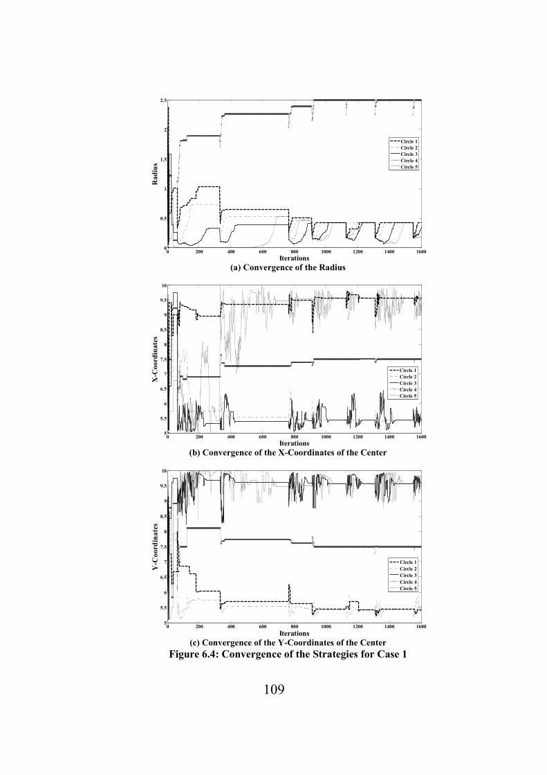
109

(a) Convergence of the Radius

(b) Convergence of the X-Coordinates of the Center

(c) Convergence of the Y-Coordinates of the Center

Figure 6.4: Convergence of the Strategies for Case 1

0 200 400 600 800 1000 1200 1400 16000

0.5

1

1.5

2

2.5

Iterations

Ra

diu

s

Circle 1

Circle 2

Circle 3

Circle 4

Circle 5

0 200 400 600 800 1000 1200 1400 16005

5.5

6

6.5

7

7.5

8

8.5

9

9.5

10

Iterations

X-C

oo

rdin

ate

s

Circle 1

Circle 2

Circle 3

Circle 4

Circle 5

0 200 400 600 800 1000 1200 1400 16005

5.5

6

6.5

7

7.5

8

8.5

9

9.5

10

Iterations

Y-C

oo

rdin

ate

s

Circle 1

Circle 2

Circle 3

Circle 4

Circle 5

110

6.2.3 Case 2: CPP with Circles Randomly Initialized

In this case of the CPP, five circles ( 5z = ) were initialized randomly in the space with

no restriction as in Case 1 where circles were randomly placed inside the square. The

length of the side of the square was five units (i.e. 5L = ). Similar to Case 1, more than 30

runs of the constrained PC algorithm described in Section 6.1 with different initial

configuration of the circles were conducted solving the Case 2. The true optimum solution

was achieved in every run with the average CPU time of 14.05 minutes and average

number of function evaluations is 68406.

The randomly generated initial solution, the intermediate iteration solutions, and the

converged true optimum solution from one of the instances of Case 2 are presented in

Figure 6.5. The corresponding convergence plot of the system objective is presented in

Figure 6.6. The convergence of the associated variables such as radius of the circles, x

coordinates and y coordinates of the center of the circles is presented in Figure 6.7(a),

6.7(b) and 6.7(c), respectively. The solution was converged at iteration 955 with 24830

function evaluations. The true optimum value of the objective function ( f ) achieved was

3.0807 units.

111

(a) Randomly generated Initial Solution (b) Solution at Iteration 301

(c) Solution at Iteration 401 (d) Solution at Iteration 601

(e) Solution at Iteration 801 (f) Stable Solution at Iteration 955

Figure 6.5: Solution History for Case 2

3 4 5 6 7 8 9 10 11 123

4

5

6

7

8

9

10

11

12

X-Coordinates

Y-C

oo

rd

ina

tes

5

1

3

2

4

4 5 6 7 8 9 10

5

5.5

6

6.5

7

7.5

8

8.5

9

9.5

10

X-Coordinates

Y-C

oord

inate

s

1

4

3

2

5

4 5 6 7 8 9 10

5

5.5

6

6.5

7

7.5

8

8.5

9

9.5

10

X-Coordinates

Y-C

oo

rdin

ate

s

2

3

4

1

5

4 5 6 7 8 9 10

5

5.5

6

6.5

7

7.5

8

8.5

9

9.5

10

X-Coordinates

Y-C

oorid

nate

s

1

2

3

4

5

4 5 6 7 8 9 10

5

5.5

6

6.5

7

7.5

8

8.5

9

9.5

10

X-Coordinates

Y-C

oo

rd

inate

s

1

2

3

4

5

4 5 6 7 8 9 10

5

5.5

6

6.5

7

7.5

8

8.5

9

9.5

10

X-Coordinates

Y-C

oo

rdin

ate

s

1

23

4

5

112

Figure 6.6: Solution Convergence Plot for Case 2

In the instance of the Case 2 presented here, the solution was perturbed at iteration 788,

988, 1170 and 1355. It is clear that the implementation of the perturbation approach at

iteration 788 helped the solution to jump out of the local minima and further achieve the

true optimum solution at iteration 955. It is important to mention that the instance

illustrated here did not require the voting heuristic to be applied.

0 200 400 600 800 1000 1200 1400-5

0

5

10

15

20

Iterations

Sy

stem

s O

bje

ctiv

e

Converged/StableSolution

113




Figure 6.7: Convergence of the Strategies for Case 2

0 200 400 600 800 1000 12000

0.5

1

1.5

2

2.5

Iterations

Ra

diu

s

Circle 1

Circle 2

Circle 3

Circle 4

Circle 5

0 200 400 600 800 1000 12005

5.5

6

6.5

7

7.5

8

8.5

9

9.5

10

Iterations

X-C

oo

rdin

ate

s

Circle 1

Circle 2

Circle 3

Circle 4

Circle 5

0 200 400 600 800 1000 12005

5.5

6

6.5

7

7.5

8

8.5

9

9.5

10

Iterations

Y-C

oo

rdin

ate

s

Circle 1

Circle 2

Circle 3

Circle 4

Circle 5

114

6.2.4 Voting Heuristic

In a few instances of the CPP cases solved here, in order to jump out of the local minimum,

a voting heuristic was required. It was implemented in conjunction with the perturbation

approach. Once the solution was perturbed, every circle voted 1 for each quadrant which it

does not belong to at all, and voted 0 otherwise. The circle with the smallest size shifted

itself to the extreme corner of the quadrant with the highest number of votes, i.e. the

winner quadrant. The new position of the smallest size circle was confirmed only when

the solution remained feasible and the algorithm continues. If all the quadrants acquire

equal number of votes, no circle moves its position and the algorithm continues. The

voting heuristic is demonstrated in Figure 6.8.

(a) A Case for Voting Heuristic (b) Voting Grids

Figure 6.8: Voting Heuristic

A voting grid corresponding to every quadrant of the square in Figure 6.8(a) is

represented in Figure 6.8(b). The solid circles represent the solution before perturbation

while corresponding perturbed ones are represented in dotted lines. The votes given by the

perturbed circles (dotted circles) to the quadrants are presented in the grid. As the

5 6 7 8 9 10

5

5.5

6

6.5

7

7.5

8

8.5

9

9.5

10

3

2

1

4

5 Q 2

1 2 3 4 5

1 1 1 0 0

Total votes = 3

Q 1

1 2 3 4 5

1 1 1 0 1

Total votes = 4

Q 3

1 2 3 4 5

1 0 0 0 1

Total votes = 2

Q 4

1 2 3 4 5

0 1 1 0 1

Total votes = 3

115

maximum number of votes are given to quadrant 1 (i.e. Q 1), the circle with smallest size

(circle 3) shifts to the extreme corner of the quadrant Q 1 and confirms the new position as

the solution remains feasible. Based on the trials conducted so far, it was noticed that the

voting heuristic was not necessary to be implemented in every run of the constrained PC

algorithm solving the CPP. Moreover, in those of the few runs in which the voting

heuristic was required, it was required to be implemented only once in the entire execution

of the algorithm. A variant of the voting heuristic was also implemented in conjunction

with energy landscape paving algorithm [32, 206, 207] in which, the smallest circle was

picked and placed randomly at the vacant place to produce a new configuration. It was

claimed that this heuristic helped the algorithm jump out of the local minima. Furthermore,

this heuristic was required to be implemented in every iteration of the algorithm.

6.2.5 Agent Failure Case

As discussed before, a centralized system is vulnerable to single point failures and its

performance may be severely affected if an agent in the system fails. On the other hand, in

case of a distributed and decentralized algorithm, the system is more robust as the system

is controlled by its autonomous subsystems.

As mentioned in section 3.2, the failed agent in PC can be considered as the one that

does not communicate with other agents in the system and does not update its probability

distribution. This does not prevent other agents from continuing further, by simply

considering the failed agent’s latest communicated strategies as the current strategies.

The immunity to agent failure is essential in the field of UAV formation and

collaborative path planning because failure of the centralized controller would be

116

devastating and may result in collision. This is addressed in the related work on UAVs [2,

56-62].

In the context of the CPP, as a variation of Case 1, circle 2 was failed at a randomly

chosen iteration 30, i.e. circle 2 does not update its x and y coordinates as well as its

radius after iteration 30. More than 30 cases of the constrained PC algorithm with

Feasibility-based Rule I were conducted solving the CPP with agent failure case and the

average function evaluations were 17365. For the case presented here, the number of

function evaluations was 19066 and the randomly generated initial solution, the

intermediate iteration solutions, and the converged true optimum solution are shown in

Figure 6.9. The corresponding convergence plot of the system objective is presented in

Figure 6.10. The convergence of the associated variables such as radius of the circles, x

coordinates and y coordinates of the center of the circles is presented in Figure 6.11(a),

6.11(b) and 6.11(c), respectively.

117

(a) Randomly generated Iteration Solution (b) Solution at Iteration 124

(c)Solution at Iteration 231 (d) Solution at Iteration 377

(e) Solution at Iteration 561 (f) Solution at Iteration 723

4 5 6 7 8 9 10 11

5

5.5

6

6.5

7

7.5

8

8.5

9

9.5

10

X-Coordinates

Y-C

oo

rdin

ate

s

1

2

3

4

5

4 5 6 7 8 9 10 11

5

5.5

6

6.5

7

7.5

8

8.5

9

9.5

10

X-Coordinates

Y-C

oo

rd

ina

tes

25

4

1

3

4 5 6 7 8 9 10 11

5

5.5

6

6.5

7

7.5

8

8.5

9

9.5

10

X-Coordinates

Y-C

oo

rdin

ate

s

2

5

4

13

4 5 6 7 8 9 10 11

5

5.5

6

6.5

7

7.5

8

8.5

9

9.5

10

X-Coordinates

Y-C

oo

rdin

ate

s2

4

5

1

3

4 5 6 7 8 9 10 11

5

5.5

6

6.5

7

7.5

8

8.5

9

9.5

10

X-Coordinates

Y-C

oo

rdin

ate

s

2

5

4

1

3

4 5 6 7 8 9 10 11

5

5.5

6

6.5

7

7.5

8

8.5

9

9.5

10

X-Coordinates

Y-C

oo

rdin

ate

s

2

5

4 3

1

118

(g) Stable Solution at Iteration 901 (h) Stable Solution at Iteration 1051

Figure 6.9: Solution History for Agent Failure Case

Figure 6.10: Convergence of the Objective Function for Agent Failure Case

4 5 6 7 8 9 10 11

5

5.5

6

6.5

7

7.5

8

8.5

9

9.5

10

X-Coordinates

Y-C

oo

rdin

ate

s

25

4

1

3

4 5 6 7 8 9 10 11

5

5.5

6

6.5

7

7.5

8

8.5

9

9.5

10

X-Coordinates

Y-C

oo

rdin

ate

s

25

4 3

1

0 200 400 600 800 1000 12004

6

8

10

12

14

16

18

20

22

Iterations

Sy

stem

Ob

ject

ive

Converged/Stable

Solutions

119




Figure 6.11: Convergence of the Strategies for Agent Failure Case

0 200 400 600 800 1000 1200 14000

0.5

1

1.5

2

2.5

Iterations

Rad

ius

Circle 1

Circle 2

Circle 3

Circle 4

Circle 5

0 200 400 600 800 1000 1200 14005

5.5

6

6.5

7

7.5

8

8.5

9

9.5

10

Iterations

X-C

oord

ina

tes

Circle 1

Circle 2

Cricle 3

Circle 4

Circle 5

0 200 400 600 800 1000 1200 14005

5.5

6

6.5

7

7.5

8

8.5

9

9.5

10

Iterations

Y-C

oord

inate

s

Circle 1

Circle 2

Circle 3

Circle 4

Circle 5

120

It is worth to mention that the voting heuristic was not required in the case presented

in Figure 6.9. This is because according to the voting heuristic the smallest circle which

moves itself to the new position is itself the failed agent. In addition, the same set of

parameter as values listed in Section 6.2.1 was used for the agent failure case.

6.3 Discussion

The above sections described the successful implementation of a generalized

constrained PC approach using a variation of the feasibility-based rule originally proposed

in [159]. The results indicated that it could successfully be used to solve constrained

optimization problems such as the CPP. It is evident from the results that the approach

was sufficiently robust and produced true optimum results in every run of Case 1 and 2. It

implies that the rational behavior of the agents could be successfully formulated and

demonstrated. Moreover, it is also evident that because of the inherent distributed nature

of the PC algorithm, it can easily accommodate the agent failure cases. The solution

highlights its strong potential to deal with the agent failure which may arise in real world

complex problems including urban traffic control, formation of airplanes fleet and mid-air

collision avoidance, etc.

In addition, the feasibility-based rule in [159, 160, 179-183] suffered from maintaining

the diversity and further required additional techniques such as niching [159], SA [160],

modified mutation approach [181, 182], and several associated trials in [179-182], etc. It

may require further computations and memory usage. On the other hand, in order to jump

out of the possible local minima, a simple perturbation approach was successfully

121

incorporated into the constrained PC algorithm. It is worth to mention that the perturbation

approach was computationally cheaper and required no additional memory usage.

It is important to mention that the concept of the avoidance of tragedy of commons was

also successfully demonstrated solving the two cases (Case 1 and Case 2) of the CPP.

More specifically, as all the agents were supposed to collectively cover the maximum

possible area within the square, every circle/agent could have in a greedy way, increased

its own radius (or size) [7, 9]. This would have further resulted into the suboptimal

solution. However, in the PC solution to the two cases of the CPP presented here, every

circle/agent selected its individual radius (or size) as well as its x and y coordinates in

order to collectively achieve the true optimum solution (i.e. collectively cover the

maximum possible area within the square) by avoiding the tragedy of commons. Although

only inequality constraints were handled in both the cases of the CPP solved here, the

approach of transformation of equality constraints into inequality constraints [172-174]

can be easily implemented for problems with equality constraints.

In agreement with the no-free-lunch theorems [213], some limitations were also

identified. The rate of convergence and the quality of the solution was dependent on the

parameters such as the number of strategies im in every agent’s strategy set

iX , the

interval factor λ and also the perturbation parameters. It is also necessary that some

preliminary trials are performed for fine-tuning these parameters. Additionally, in order to

confirm the convergence, the algorithm was required to be run beyond the convergence for

a considerable number of iterations.

122

The following sections discuss the Feasibility-based Rule II, associated formulation,

implementation and validation of results solving three cases of the Sensor Network

Coverage Problem (SNCP).

6.4 Feasibility Based Rule II

This rule is a variation of the Feasibility-based Rule I discussed in Section 6.1 and also

allows the objective function and the constraint information to be considered separately. In

addition to the iterative tightening of the constraint violation tolerance in order to obtain

fitter solution and further drive the convergence towards feasibility, the Feasibility based

Rule II helps the solution jump out of possible local minima.

At the beginning of the PC algorithm, the number of constraints improved µ is

initialized to zero, i.e. 0µ = . The value of µ is updated iteratively as the algorithm

progresses. Similar to the Feasibility-based Rule I, Feasibility-based Rule II is also

assisted with the modified approach of updating of the sampling space as well as the

convergence criterion. The rule and these assisting techniques are discussed below as the

modifications to the unconstrained PC approach presented in Section 3.4.


The step 5 of the unconstrained PC procedure discussed in Section 3.4 is modified by

using the following rule:

(a) Any feasible solution is preferred over any infeasible solution

(b) Between two feasible solutions, the one with better objective is preferred

123

(c) Between two infeasible solutions, the one with more number of improved

constraint violations is preferred.

(d) If the solution remains feasible and unchanged for successive predefined number

of iterations, and current feasible system objective is worse than the previous

iteration feasible solution, accept the current solution. Similar to SA [95-97, 185],

this may help jump out of the local minima.

The detailed formulation of the above rule is explained below and further presented in

window A of the constrained PC algorithm flowchart in Figure 6.12.

(a) If the current system objective [ ]( )fav

G Y as well as the previous solution are



Y

as current solution if the number of improved constraints is greater than or equal to

µ , i.e. improvedC µ≥ , and then the value of µ is updated to

improvedC , i.e.

improvedCµ = .

(b) If the current system objective [ ]( )fav

G Y is feasible, and the previous solution is



Y

as the current solution, and then the value of µ is updated to 0, i.e.

0improvedCµ = = .

(c) If the current system objective [ ]( )fav

G Y is feasible and is not worse than the

previous feasible solution, accept the current system objective [ ]( )fav

G Y and


Y as the current solution.

124

(d) If all the above conditions (a) to (c) are not met, then discard current system

objective [ ]( )fav


Y , and retain the previous iteration

solution.

(e) If the solution remains feasible and unchanged for successive pre-specified testn

iterations i.e. [ ],( )fav n

G Y and [ ],( )testfav n nG

−Y are feasible and

[ ] [ ], ,( ) ( )testfav n fav n n

G G−=Y Y , and the current feasible system objective is worse than

the previous iteration feasible solution, accept the current system objective

[ ]( )

favG Y and corresponding

[ ]favY as the current solution.

In this way the algorithm progresses by iteratively tightening the constraint violation.


It is important to mention that once the solution becomes feasible, every agent i

shrinks its sampling interval to the local neighborhood of its current favorable strategy

[ ]fav

iX . This is done as follows:


i i down i i i down i iX Xλ λ Ψ ∈ − Ψ −Ψ + Ψ −Ψ

, 0 1downλ< ≤

(6.15)

where downλ is referred to as the interval factor corresponding to the shrinking of sample

space. The modification of updating the sampling space is presented in window B of the

constrained PC algorithm flowchart in Figure 6.12. The associated modified convergence

criterion is discussed below.

125


The detailed formulation of the modified convergence criterion is explained below and

further presented in window C of the constrained PC algorithm flowchart in Figure 6.12.

The current system objective [ ],( )fav n

G Y and corresponding [ ],fav n

Y are accepted as the

final solution referred to as [ ],( )fav final

G Y and

[ ] [ ] [ ] [ ] [ ]{ }, , , , ,


! !X X X X−=Y , respectively, if and only if any of

the following conditions are satisfied.

(a) If temperature finalT T= or 0T →

(b) If maximum number of iterations exceeded

(c) If there is no significant change in the system objective (i.e.

[ ] [ ], , 1( ) ( )

fav n fav nG G ε−− ≤Y Y ) for successive considerable number of iterations.

126

Figure 6.12: Constrained PC Algorithm Flowchart (Feasibility-based Rule II)

Discard current and

retain previous


related strategies

current feasible system

objective ≤ previous

feasible system objective?

N

1n n= + ,

TT T Tα= −

Solution is

unchanged for

successive testn

iterations ?

START

For every agent i set up a strategy set with im strategies, assign uniform probabilities to

every agent’s strategies, initialize n , T , µ and global sampling interval for all the

N Y Convergence?

Accept the system

objective as final

solution along with

agents’ associated

strategies

Update the sampling

interval of every agent i

to its local neighborhood

STOP

Accept current

objective function


Compute the system objective function and associated constraints

Form the Homotopy function for each agent

Form mi combined strategy sets associated with every agent compute mi objective

Is the solution

feasible?

N Y

number of improved

constraints ≥ previous

solution constraints?

Y N Y

Accept current

objective function


Discard current and

retain previous


related strategies

Update the global

sampling interval

Y

N

A

B

C

Compute mi objective functions and associated expected local objectives for each agent

For each agent minimize the Homotopy function using BFGS method and obtain the

probability distribution for every agent identifying its favorable strategy

127

6.5 The Sensor �etwork Coverage Problem (S�CP)

The sensor network plays a significant role in various strategic applications such as

hostile and hazardous environmental and habitat exploration and surveillance, critical

infrastructure monitoring and protection, situational awareness of battlefield and target

detection, natural disaster relief, industrial sensing and diagnosis, biomedical health

monitoring, seismic sensing, etc. [35-43]. The deployment or positioning of the individual

sensor directly affects the coverage, detection capability, connectivity and associated

communication cost and resource management of the entire network [37, 38, 44, 214].

According to [39, 44, 215-217], coverage is the important performance metric that

quantifies the quality and effectiveness of the surveillance/monitoring provided by the

sensor network. This highlighted the requirement for an effective sensor deployment

algorithm to optimize the coverage of the entire network [39, 44, 214]. Furthermore,

according to [218, 219] the connected coverage is important by which all the sensors in

the network can communicate with one another over multiple hops.

The sensor network coverage can be classified as deterministic or stochastic coverage

[220]. The deterministic coverage refers to the static deployment of the sensors over a

predefined Field of Interest (FoI) [221-225]. It includes the uniform coverage of the FoI as

well as weighted coverage of certain section of the FoI [45, 216]. The stochastic coverage

refers to the random deployment of the sensors over the FoI. The sensor positions are

selected based on the uniform, Gaussian, Poisson or any other problem specific

distribution [216]. The deterministic coverage may provide worst-case performance which

may not be achievable by stochastic coverage [39, 217]. According to [226], the coverage

can also be classified into three types. The first is blanket coverage, which represents the

128

static arrangement of the sensors to maximize the total detection area; the second is barrier

coverage, which aims to arrange the sensors to form a barrier in order to minimize the

probability of undetected penetration/intrusion through the barrier [217, 227]; and the

third is sweep coverage which is a moving barrier of sensors that aims to maximize the

number of detections per unit time and minimize the number of missed detections per unit

area. The blanket coverage can be further classified into two types [35]. The first is point-

set coverage, which aims to cover a set of discrete points scattered over a certain field and

the second is FoI coverage, which aims to cover a certain region to the maximum possible

extent.

This following section addresses the problem of deployment of a set of homogeneous

(identical characteristics) sensors over a certain predefined FoI in order to achieve the

maximum possible deterministic connected blanket coverage using the method of PC.

6.5.1 Formulation of the S�CP

The SNCP addressed here is as follows: given a set of z homogeneous sensors with equal

and fixed sensing range sr for every sensor { }1, 2,...,i z∈ , and the sensing area of every

sensor i modeled as a circle with the sensor located at its centre; find the deployment of

all the sensors to collectively cover the maximum possible area (hereafter referred to as

collective coverage collectiveA ) of a square FoI without overlapping one another and without

exceeding the boundaries of the square FoI, and importantly maintaining connectivity

between them. The connectivity here refers to the constraint which limits the distance

( ),d i j between two adjacent sensors i and j to a maximum predefined value γ , i.e.

( ),d i j γ≤ , , , , 1,2,...,i j i j i j z≠ =∼ [218, 219] where adjacency is represented by

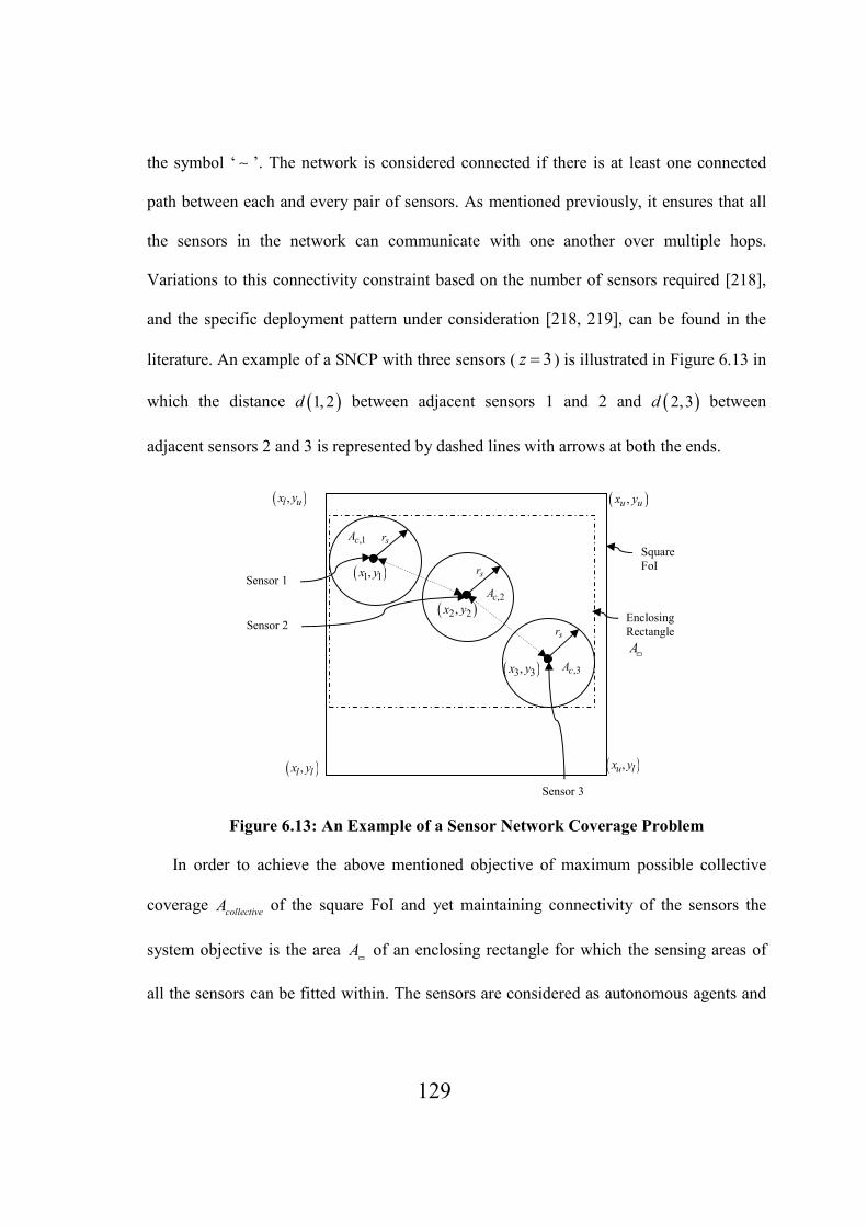
129

the symbol ‘ ∼ ’. The network is considered connected if there is at least one connected

path between each and every pair of sensors. As mentioned previously, it ensures that all

the sensors in the network can communicate with one another over multiple hops.

Variations to this connectivity constraint based on the number of sensors required [218],

and the specific deployment pattern under consideration [218, 219], can be found in the

literature. An example of a SNCP with three sensors ( 3z = ) is illustrated in Figure 6.13 in

which the distance ( )1, 2d between adjacent sensors 1 and 2 and ( )2,3d between

adjacent sensors 2 and 3 is represented by dashed lines with arrows at both the ends.

Figure 6.13: An Example of a Sensor �etwork Coverage Problem

In order to achieve the above mentioned objective of maximum possible collective

coverage collectiveA of the square FoI and yet maintaining connectivity of the sensors the

system objective is the area A▭

of an enclosing rectangle for which the sensing areas of

all the sensors can be fitted within. The sensors are considered as autonomous agents and

( ),l lx y

( ),u ux y

( ),u lx y

sr

sr

Sensor 3

,1cA

,2cA

Square

FoI ( )1 1,x y

Enclosing

Rectangle

A▭

( ),l ux y

( )2 2,x y

,3cA ( )3 3,x y

sr Sensor 2

Sensor 1

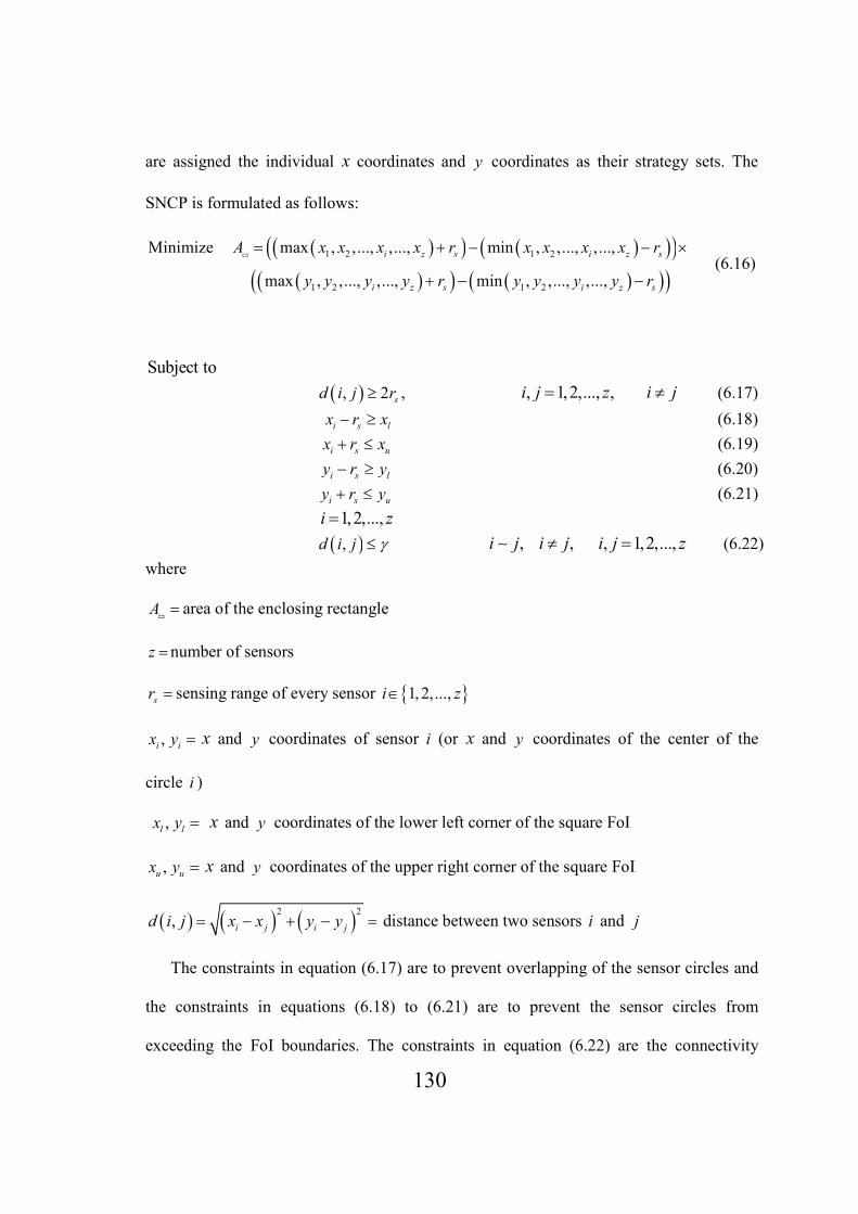
130

are assigned the individual x coordinates and y coordinates as their strategy sets. The

SNCP is formulated as follows:

( )( ) ( )( )( )( )( ) ( )( )( )

1 2 1 2

1 2 1 2

Minimize max , ,..., ,..., min , ,..., ,...,

max , ,..., ,..., min , ,..., ,...,

i z s i z s

i z s i z s

A x x x x r x x x x r

y y y y r y y y y r

= + − − ×

+ − −

▭

(6.16)

Subject to

( ), 2 sd i j r≥ , , 1,2,..., ,i j z i j= ≠ (6.17)

i s lx r x− ≥ (6.18)

i s ux r x+ ≤ (6.19)

i s ly r y− ≥ (6.20)

i s uy r y+ ≤ (6.21)

1,2,...,i z= ( ),d i j γ≤ , , , 1,2,...,i j i j i j z≠ =∼ (6.22)

where

A =▭

area of the enclosing rectangle

z =number of sensors

sr = sensing range of every sensor { }1,2,...,i z∈

,i ix y = x and y coordinates of sensor i (or x and y coordinates of the center of the

circle i )

,l lx y = x and y coordinates of the lower left corner of the square FoI

,u ux y = x and y coordinates of the upper right corner of the square FoI

( ) ( ) ( )2 2

, i j i jd i j x x y y= − + − = distance between two sensors i and j

The constraints in equation (6.17) are to prevent overlapping of the sensor circles and

the constraints in equations (6.18) to (6.21) are to prevent the sensor circles from

exceeding the FoI boundaries. The constraints in equation (6.22) are the connectivity

131

constraints and are checked in every iteration using the well known Depth First Search

(DFS) algorithm [228] only when all the other constraints are satisfied.

The associated collective coverage collectiveA is calculated as follows:

,

1

z

collective c i

i

A A=

=∑ (6.23)

where ,c iA =

FoI coverage achieved by sensor i

In the three sensor example illustrated in Figure 6.13, the individual sensor coverage

area is 2

,c i sA rπ= and the collective coverage is 3

2

,

1

3collective c i s

i

A A rπ=

= =∑ . However, there

can be many possible instances where the sensing areas of the sensors may not be

completely within the FoI, and the required computation for these different individual

sensor coverage cases are discussed in Appendix D.

6.5.2 Variations of the S�CP Solved

In solving the SNCP using constrained PC approach, the sensors were considered as

autonomous agents. These sensors were assigned the individual x coordinates and y

coordinates as their strategy sets. Two variations of the SNCP were solved. In Variation 1,

the number of sensors and their sensing ranges were chosen such that the area A▭

of the

converged enclosing rectangle should be significantly lesser than the area of the square

FoI being covered. Unlike Variation 1, in Variation 2 the number of sensors and the

associated sensing range were chosen such that the area A▭

of the converged enclosing

rectangle will be significantly larger than the area of the square FoI being covered. Three

cases of Variation 2 were solved. These cases differ from one another based on the

132

sensing range of the sensors as well as the number of sensors being deployed to cover the

square FoI.

In both the variations, sensors were randomly located in-and-around the square FoI

and all the constraints presented in equations (6.17) to (6.21) were treated using the

feasibility-based approach described in Section 6.4. It is important to mention here that on

satisfying the inter-agent overlapping constraints presented in equation (6.17) the

sampling space of every individual agent was shrunk to its local neighborhood. The

approach of shrinking the sampling space is discussed in equation (6.15).

The constrained PC algorithm solving both the variations was coded in MATLAB

7.8.0 (R2009A) and the simulations were run on a Windows platform using an Intel Core

2 Duo, 3GHz processor speed and 3.25GB memory capacity. Furthermore, for both the

variations the set of parameters chosen was as follows: (a) individual agent sample size

5im = , (b) the shrinking interval factor 0.05downλ = , (c) number of test iterations

20testn = . In addition, the maximum allowable distance between two adjacent sensors γ

was chosen as 0.2 2 sr+ units.

6.5.2.1 Variation 1

In this variation of the SNCP, five sensors ( 5z = ) each with sensing radius 0.5

( 0.5sr = ) units were initialized randomly in-and-around a square FoI. The length of the

side of the square FoI was five units. In total, 10 runs of the constrained PC algorithm

described in Section 6.4 with different initial locations of the sensors were performed. The

summary of results including the average CPU time, average number of function

133

evaluations, the minimum, maximum and average values of the collective coverage

achieved and the area of the enclosing rectangle are listed in Table 6.1.

The iterative progress of the solution including randomly generated initial solution (the

set of gray circles) and converged optimum solution (the set of black circles) from one of

the instances solving Variation 1 is presented in Figure 6.14. The corresponding

convergence plot of the area of the enclosing rectangle is presented in Figure 6.15(a) and

the convergence plot of the associated collective coverage is presented in Figure 6.15(b).

It is clear from these convergence plots that the solution was converged at iteration 2198.

6.5.2.2 Variation 2

Three distinct cases of Variation 2 were solved. Case 1 includes five sensors ( 5z = )

each with sensing radius 1.2 ( 1.2sr = ), Case 2 includes ten sensors ( 10z = ) each with

sensing radius 1 ( 1sr = ) and Case 3 includes twenty sensors ( 20z = ) each with sensing

radius 0.6 ( 0.6sr = ) units. In each of the three cases, sensors were initialized randomly in-

and-around the square FoI. The length of the side of the square FoI was five units. In total,

10 runs of the constrained PC algorithm described in Section 6.4 with different initial

locations of the sensors were conducted for each of the three cases.

The iterative progress of the solution including randomly generated initial solution (the

set of gray circles) and the converged optimum solution (the set of black circles) from one

of the instances each of Case 1, 2 and 3 are illustrated in Figure 6.16, 6.18 and 6.20,

respectively. In addition, the corresponding convergence plots of the area of the enclosing

rectangle are presented in Figure 6.17(a), 6.19(a) and 6.21(a), and the convergence plots of

the collective coverage are presented in Figure 6.17(b), 6.19(b) and 6.21(b), respectively.

134

It is clear from these convergence plots that the solution for Case 1, Case 2 and Case 3

was converged at iteration 6725, 17484 and 42218, respectively.

The summary of results corresponding to Case 1, 2 and 3 are listed in Table 6.1.

Table 6.1: Summary of Results Sr. �o Particulars Variation 1 Variation 2

1 Cases -- Case 1 Case 2 Case 3

2 Number of Sensors ( z ) 5 5 10 20

3 The Sensing Range ( sr ) 0.5 1.2 1 0.6

4 Average Collective Coverage 3.927 18.5237 19.4856 16.3631

5 Minimum and Maximum

Collective Coverage

3.9270,

3.9270

18.0920,

18.7552

17.5427,

20.8797

15.5347,

17.3377

6 Standard Deviation associated with

Collective Coverage

0.0000 0.1687 1.1837 1.2217

7 Average area of the Enclosing

Rectangle

5.8311 34.3014 49.0938 39.3480

8 Minimum and Maximum area of

the Enclosing Rectangle

5.7046,

5.9750

33.0448,

39.7099

44.7135,

52.6277

34.1334,

43.8683

9 Standard Deviation associated with

the area of Enclosing Rectangle

0.1040 1.9899 2.6995 2.8829

10 Average CPU time (Approx.) 20 Mins 1 Hr 2Hrs 3.5 Hrs

11 Average number of Function

Evaluations

90417 315063 1172759 3555493

Figure 6.14: Solution History for Variation 1

5 6 7 8 9 10 11

4

5

6

7

8

9

10

11

X-Coordinates

Y-C

oord

inate

s

135

(a) Convergence of the Area of the Enclosing Rectangle

(b) Convergence of the Collective Coverage

Figure 6.15: Convergence of the Area of the Enclosing Rectangle and Collective

Coverage for Variation 1

0 500 1000 1500 2000 2500 30005

10

15

20

25

30

35

40

45

Iterations

Are

a o

f th

e E

ncl

osi

ng

Rect

an

gle

0 500 1000 1500 2000 2500 30000

0.5

1

1.5

2

2.5

3

3.5

4

Iterations

Co

llecti

ve C

ov

era

ge

136

Figure 6.16: Solution History for Case 1 of Variation 2

2 4 6 8 10 12 14

2

4

6

8

10

12

14

X-Coordinates

Y-C

oo

rdin

ate

s

137

(a) Convergence of Area of the Enclosing Rectangle



Coverage for Case 1 of Variation 2

0 1000 2000 3000 4000 5000 6000 7000 800020

40

60

80

100

120

140

160

180

200

220

Iterations

Area

of

the E

nclo

sin

g R

ecta

ng

le

0 1000 2000 3000 4000 5000 6000 7000 80000

2

4

6

8

10

12

14

16

18

Iterations

Co

llect

ive C

ov

era

ge

138


2 4 6 8 10 12 140

2

4

6

8

10

12

14

X-Coordinates

Y-C

oo

rd

ina

tes

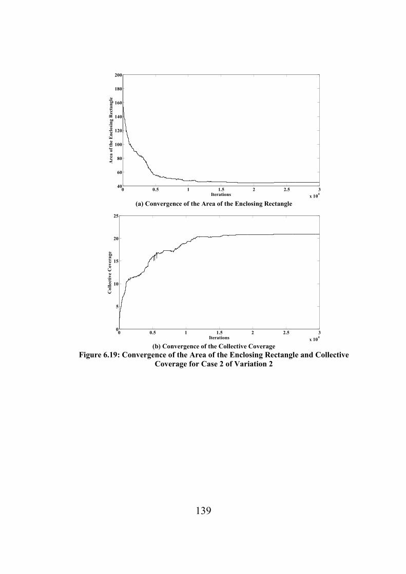
139





0 0.5 1 1.5 2 2.5 3

x 104

40

60

80

100

120

140

160

180

200

Iterations

Area

of

the E

nclo

sin

g R

ecta

ng

le

0 0.5 1 1.5 2 2.5 3

x 104

0

5

10

15

20

25

Iterations

Co

llec

tiv

e C

ov

era

ge

140


0 2 4 6 8 10 120

2

4

6

8

10

12

14

X-Coordinates

Y-C

oo

rd

ina

tes

141





6.6 Discussion

The above solutions using constrained PC indicated that it could successfully be used

to solve constrained optimization problems such as the SNCP. Moreover, connectivity

constraint was satisfied in every run of the constrained PC solving the SNCP. It is worth to

mention that the DFS algorithm was successfully implemented for checking the

connectivity constraint. It is evident from the results presented in Table 6.1, that the

0 0.5 1 1.5 2 2.5 3 3.5 4 4.5

x 104

20

40

60

80

100

120

140

160

180

200

Iterations

Area

of

the E

nclo

sin

g R

ecta

ng

le

0 0.5 1 1.5 2 2.5 3 3.5 4 4.5

x 104

0

2

4

6

8

10

12

14

16

18

Iterations

Co

llec

tiv

e C

ov

era

ge

142

approach produced sufficiently robust results solving all the variations of the SNCP. It

implies that the rational behavior of the agents could be successfully formulated and

demonstrated. It is important to highlight that the distributed nature of the PC approach

will allow the total number of function evaluations to be equally divided among the agents

of the system. This can be made practically evident by implementing the PC approach on

a real distributed platform assigning separate workstations carrying out the computations

independently. These advantages along with the directly incorporated uncertainty using

the real valued probabilities treated as variables suggest that PC can potentially be applied

to real world complex problems.

In addition, the feasibility-based rule in [159, 160, 179-183] suffered from maintaining

the diversity and further required additional techniques such as niching [159], SA [160],

modified mutation approach [181, 182], and several associated trials in [179-182], etc. It

may require further computations and memory usage. Moreover, in order to jump out of

local minima, feasibility-based Rule I was required to be accompanied with a perturbation

approach which required several associated parameters to be tuned. In case of the

Feasibility-based Rule II proposed in Section 6.4, the perturbation approach was

completely replaced by the addition of a generic rule of accepting the worse feasible

solution when the solution remains feasible and unchanged for a successive predefined

number of iterations. From the convergence plot and the associated results it is evident

that this additional generic rule helped the solution jump out of local minima.

In agreement with the no-free-lunch theorems [213], some limitations were also

identified. The rate of convergence and the quality of solution was dependent on the

parameters such as the number of strategies im in every agent’s strategy set

iX , the

143

interval factor downλ and the number of test iterations

testn . It necessitated some

preliminary trials for fine-tuning these parameters. Additionally, a high computational cost

achieving the optimum solution was noticed. However, computational time can be reduced

by implementing the PC approach on an actual distributed platform.

144

CHAPTER 7

CO�CLUSIO�S A�D RECOMME�DATIO�S

7.1 Conclusions

The PC methodology was improved and demonstrated successfully within a COIN

framework. The original PC approach was improved with a reduction in the computational

complexity. A scheme for updating the solution space was developed which contributed to

faster convergence and improved efficiency of the overall algorithm. In addition, PC was

assumed to be converged when there was no further improvement in the final goal and/or

exceeds a predefined number of iterations. The modified PC algorithm was validated

successfully optimizing the Rosenbrock Function.

Moreover, various inherent and desirable characteristics of the PC methodology of

being a distributed, decentralized and cooperative approach were investigated and

exploited. This includes the successful demonstration of the important characteristic of

avoidance of tragedy of commons as well as the capability of PC to deal with the failure of

a subsystem or an agent. Furthermore, the concept of Nash equilibrium was successfully

formalized and demonstrated.

In the attempts to exploit the key characteristics and benefits of the PC methodology of

being distributed, decentralized and cooperative approach as well as make it a more

generic and powerful optimization approach, a number of constraint handling techniques

in the form of penalty function and feasibility-based rules were developed for

incorporating into the overall algorithm. These techniques were tested and validated by

successfully solving a number of challenging problems from variegated areas.

145

In the first attempt to develop a constraint handling technique, several problem specific

heuristic techniques were proposed and incorporated into the PC algorithm solving the

challenging NP-hard Multiple Depot Multiple Traveling Salesmen Problem (MDMTSP)

and Single Depot Multiple Traveling Salesmen Problem (SDMTSP). The implementation

of these techniques helped the algorithm to converge faster as well as to jump out of local

minima. It is worth to mention that for the first time the MDMTSP and the SDMTSP were

solved using a distributed, decentralized and cooperative approach such as PC. The true

optimum solution was produced in every run of the PC solving two specially developed

test cases of the MDMTSP. The MDMTSP and SDMTSP were solved in a reasonably

short time.

In the second attempt, a generalized constrained PC approach was proposed using the

simple penalty function method. The dependence on the penalty parameter was reduced

through the approach of iteratively biasing the fitter solution, i.e. iteratively tightening the

tolerance to constraint violation. The constrained PC approach was tested successfully on

a variety of optimization problems with equality and inequality constraints. It could

produce competitive, if not better, results and appeared to be a promising distributed

approach capable of handling the constraints.

In the third attempt, two variations of the Feasibility-based Rule were proposed. The

Feasibility-based Rule I was successfully formalized and demonstrated for solving two

cases of the Circle Packing Problem (CPP). In both the cases, the approach could find the

true optimal solution in every run of the constrained PC in reasonable computational

efforts. Similar to the penalty function approach, the constraint violation tolerance was

iteratively tightened in order to obtain the fitter solution. In addition to the two test cases,

146

the potential of PC was successfully tested for the case of agent failure which yielded

promising results. It is worth to mention here that in order to make the solution jump out

of possible local minima and further reach the true optimum, the rule was assisted with the

perturbation approach as well as the problem specific voting heuristic. Most importantly,

the PC solution to the CPP successfully demonstrated the important and desirable

characteristic in the PC algorithm of avoiding the tragedy of commons.

The Feasibility-based Rule II was successfully applied for solving two variations of the

SNCP. Furthermore, the constrained PC approach produced sufficiently robust results

solving all the variations of the SNCP. It is important to mention that the Feasibility-based

rule II did not require the perturbation approach to be implemented for the solution to

jump out of local minima. In addition, in the solution procedure of the SNCP, the depth-

first-search algorithm was successfully implemented. Furthermore, in solving the CPP and

the SNCP, the BFGS method was successfully used as an alternative to the existing

Nearest Newton Descent Scheme for minimizing the Homotopy function.

Besides the above discussed improvements in the PC algorithm, a few disadvantages

were also identified. A high computational cost was required in achieving the optimum

solution. However, real (wall clock) time can be reduced by implementing the PC

approach on an actual distributed (parallel) platform. Furthermore, the rate of convergence

and the quality of solution was dependent on a few parameters. This necessitated a few

preliminary trials for the fine-tuning of these parameters.

According to the no-free-lunch theorem [175, 213], making a few assumptions about

the set of problems being solved may make the search technique and associated constraint

handling method more effective and efficient in solving those problems; however, the

147

possibility of performing worse or being trapped into local minima for other problems

may be greater. It is important to mention here that in agreement with the no-free-lunch

theorem, along with the preliminary trials for fine tuning of a few parameters, in order to

make the PC algorithm jump out of possible local minima, various problem specific

heuristic techniques were required to be developed and further incorporated into the PC

algorithm.

7.2 Recommendations for Future Work

For future work, efforts will be taken to make the approach more generalized and

increase the efficiency of the PC algorithm. This may include improving the

diversification of sampling, the rate of convergence, computational cost, quality of results,

etc. by developing a self adaptive scheme for the parameters such as the number of

strategies im and interval factor λ and temperature step size

Tα . In addition, a local

search technique can be incorporated for assisting in a neighborhood search to reach the

global optimum.

The author is also interested to extend and modify the PC methodology further to make

it capable of solving a variety of discrete problems which may open up a wider range of

applications including complex mechanical design and assembly problems [229-232] as

well as disassembly problems [233]. In addition, the author also sees the potential of

constrained PC approach for the design of composite structures with various

manufacturing constraints [234].

In order to exploit its property of being distributed, the constrained PC approach can

be used for solving more realistic and large size problems such as machine shop

148

scheduling, urban traffic control, etc. The author also sees some potential in the field of

healthcare systems management [235]. In addition, more realistic path planning problems

of the Multiple Unmanned Vehicles (MUVs) can then be solved with the MTSP and VRP

approaches.

As a continuation and further development/improvement in the constraint handling

technique, the author is currently working on the Multi-Objective Probability Collectives

(MOPC) approach. The constraints in this approach are being considered as objectives to

be optimized along with the system objective. The approach of considering constraints as

objectives is inspired from similar work done in [172-174, 236] using GA. A short

discussion on the MOPC approach as well as the potential of PC in urban traffic control is

discussed in the following sections.

7.2.1 Multi-Objective Probability Collectives (MOPC)

As mentioned previously, the Evolutionary Algorithms (EAs) in general are

unconstrained optimization techniques and their performance may be significantly

affected when constraints are involved. Recently, some researchers [172-174, 237-245]

have proposed the Multi-Objective optimization concept to handle the single objective

constrained problems in which the constraints are treated as objectives to be optimized.

This allows for the unconstrained optimization of every objective and further may provide

the decision maker a set of candidate solutions. According to [235], this may allow the

decision maker to deal with the soft constraints, i.e. a choice can be made from a set of

candidate solutions with a slight constraint violation and substantial improvement in the

objective function value. In addition, according to [238], the EAs when resort to this

149

Multi-Objective optimization approach, it is possible to quickly locate the feasible region

but the extension to solve the single objective constrained problems is not straightforward.

In order to exploit above mentioned benefits the author of this thesis is currently

working on applying the PC approach to address the Multi-Objective optimization

approach solving the single objective constrained problems. Moreover, as per the

knowledge of the author, this approach is never addressed in a distributed way. This may

also help the solution to exploit the benefits associated with the distributed approach such

as PC. In addition, the author intends to test the approach solving a variety of multi-

objective test problems [246] as well as challenging machine shop scheduling problem

[247].

7.2.2 PC for the Urban Traffic Control

In recent years, the ever growing traffic volume in urban areas motivated several

researchers to address the traffic control problem as an optimization problem. Some of the

researchers proposed traffic responsive controllers by focusing on a single intersection

traffic light optimization, by isolating it from other neighboring intersections [248-255].

As the load on the traffic network increases, the performance of the traffic responsive

controller decreases and tends to resemble that of a fixed-time controller [256, 257-259].

Moreover, such systems are difficult to set up, maintain and demand significant

computing power [260]. The ever growing traffic in urban areas and above mentioned

limitations triggered the need for a distributed control of the traffic at the corresponding

intersections [261, 262].

150

In the effort of solving the traffic control problem using PC, a network of intersections

can be considered. The PC approach can be applied to a predefined network of

intersections. Each intersection can be represented as an agent deciding its own variable

values such as green signal duration as well as the phase sequence by considering the

traffic condition at the neighboring intersections in the network. The application of PC

solving the traffic control problem may help to exploit the inherent characteristics of PC

discussed in Section 3.2 and may further open the doors for applying the PC to real world

complex problems.

151

APPE�DIX A

Analogy of Homotopy Function to Helmholtz Free Energy

A.1 The Homotopy function ( )( ),i iJ q TX is analogous to the Helmholtz free energy in

statistical physics [100-106]. The Helmholtz free energy equation can be represented

as follows [106]:

L D TS= − (A.1)

where L is Helmholtz free energy available to do the work or to create a system

when the environment is at temperature T . The term D is referred to as internal

energy and S is the entropy of the physical system. The term TS is the spontaneous

energy that can be transferred from the environment to the system.

As Helmholtz free energy L is actually the measure of the amount of internal

energy D needed to create the system, achieving thermal equilibrium is nothing but

minimizing the free energy L at temperature T , and hence directly minimizing the

internal energy D . The procedure involves a series of iterations gradually reducing

the entropy level of the system. This suggests the framework of an annealing schedule,

i.e. start at a high temperature 0T >> or initialT T= and successively reducing the

temperature and the entropy level, achieving the thermal equilibrium at every

successive temperature drop until 0T → or finalT T= . This process avoids the local

minima of internal energy D and reaches the global minima at 0T → or finalT T= .

A.2 The analogy of the Homotopy function ( )( ),i iJ q TX to Helmholtz free energy L in

statistical physics is the motivation behind minimizing the collection of system

152

objectives [ ]

1

( )im

r

i

r

G=∑ Y [100-104]. As thermal equilibrium needs to be achieved to

minimize the free energy L of the physical system given in equation (A.1), similarly,

the equilibrium needs to be achieved to minimize the Homotopy function

( )( ),i iJ q TX and that is referred to as Nash equilibrium.

According to [102, 103], careful annealing of physical systems ensures the

convergence to the global minimum of the energy D . One of the most suitable

approaches to deal with the Homotopy function such as ( )( ),i iJ q TX and eventually

the collection of system objectives [ ]

1

( )im

r

i

r

G=∑ Y having many possible local minima is

referred to as Deterministic Annealing (DA).

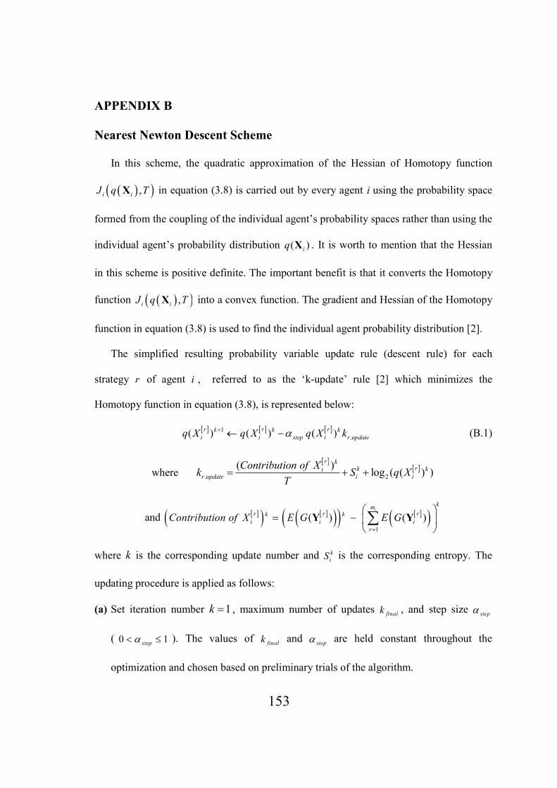
153

APPE�DIX B

�earest �ewton Descent Scheme

In this scheme, the quadratic approximation of the Hessian of Homotopy function

( )( ),i iJ q TX in equation (3.8) is carried out by every agent i using the probability space

formed from the coupling of the individual agent’s probability spaces rather than using the

individual agent’s probability distribution ( )iq X . It is worth to mention that the Hessian

in this scheme is positive definite. The important benefit is that it converts the Homotopy

function ( )( ),i iJ q TX into a convex function. The gradient and Hessian of the Homotopy

function in equation (3.8) is used to find the individual agent probability distribution [2].

The simplified resulting probability variable update rule (descent rule) for each

strategy r of agent i , referred to as the ‘k-update’ rule [2] which minimizes the

Homotopy function in equation (3.8), is represented below:

[ ] [ ] [ ]1

.( ) ( ) ( )r r rk k k

i i step i r updateq X q X q X kα+ ← − (B.1)

where [ ]

[ ]. 2

( )log ( ( ) )

r krk ki

r update i i

Contribution of Xk S q X

T= + +

and [ ]( ) [ ]( )( ) [ ]( )1

( ) ( )i

km

r r rk k

i i i

r

Contribution of X E G E G=

= −

∑Y Y

where k is the corresponding update number and k

iS is the corresponding entropy. The

updating procedure is applied as follows:

(a) Set iteration number 1k = , maximum number of updates finalk , and step size

stepα

( 0 1stepα< ≤ ). The values of finalk and

stepα are held constant throughout the

optimization and chosen based on preliminary trials of the algorithm.

154

(b) Update every agent’s probability distribution ( )( )

k

iq X using the update rule in

equation (B.1).

(c) If finalk k≥ , stop, else update 1k k= + and return to (b).

For each agent i , the above optimization process converges to a probability variable

vector ( )iq X which can be seen as the individual agent’s probability distribution clearly

distinguishing every strategy’s contribution towards the minimization of the expected

collection of system objectives ( )[ ]

1

( )im

r

i

r

E G=∑ Y . In other words, for every agent i , if

strategy r contributes the most towards the minimization of the objective than other

strategies, its corresponding probability certainly increases by some amount more than

those for the other strategies’ probability values, and so strategy r is distinguished from

the other strategies. Such a strategy is referred to as a favorable strategy [ ]fav

iX .

The initial uniform probability distribution, the intermediate iteration distributions, and

the converged probability distribution clearly distinguishing the contribution of every

strategy from one of the runs solving the tension/compression spring design problem

discussed in Chapter 5 are illustrated in Figure B.1.

155

(a) (b)

(c) (d)

(e)

Figure B.1: Solution History of Probability Distribution using �earest �ewton

Descent Scheme

0 5 10 15 20 25 30 35 40 45 500

0.005

0.01

0.015

0.02

0.025

Strategy

Prob

ab

ilit

y

0 5 10 15 20 25 30 35 40 45 500

0.005

0.01

0.015

0.02

0.025

0.03

0.035

Strategy

Prob

ab

ilit

y

0 5 10 15 20 25 30 35 40 45 500

0.02

0.04

0.06

0.08

0.1

0.12

Strategy

Pro

ba

bil

ity

0 5 10 15 20 25 30 35 40 45 500

0.05

0.1

0.15

0.2

0.25

0.3

0.35

0.4

0.45

0.5

Strategy

Pro

ba

bil

ity

0 5 10 15 20 25 30 35 40 45 500

0.1

0.2

0.3

0.4

0.5

0.6

0.7

0.8

0.9

1

Strategy

Pro

bab

ilit

y

Favorable

Strategy

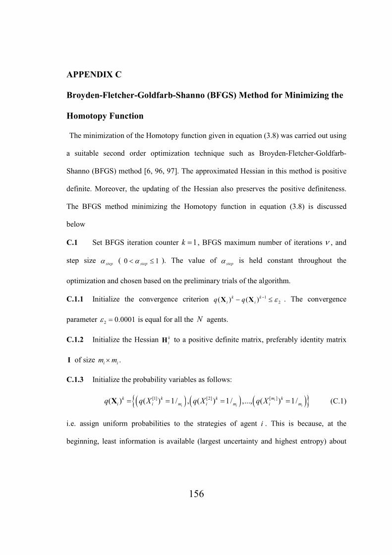
156

APPE�DIX C

Broyden-Fletcher-Goldfarb-Shanno (BFGS) Method for Minimizing the

Homotopy Function

The minimization of the Homotopy function given in equation (3.8) was carried out using

a suitable second order optimization technique such as Broyden-Fletcher-Goldfarb-

Shanno (BFGS) method [6, 96, 97]. The approximated Hessian in this method is positive

definite. Moreover, the updating of the Hessian also preserves the positive definiteness.

The BFGS method minimizing the Homotopy function in equation (3.8) is discussed

below

C.1 Set BFGS iteration counter 1k = , BFGS maximum number of iterations ν , and

step size stepα ( 0 1stepα< ≤ ). The value of

stepα is held constant throughout the

optimization and chosen based on the preliminary trials of the algorithm.

C.1.1 Initialize the convergence criterion 1

2( ) ( )k k

i iq q ε−− ≤X X . The convergence

parameter 2 0.0001ε = is equal for all the ! agents.

C.1.2 Initialize the Hessian k

iH to a positive definite matrix, preferably identity matrix

I of size i im m× .

C.1.3 Initialize the probability variables as follows:

( ) ( ) ( ){ }[ ][1] [2]( ) ( ) 1/ , ( ) 1/ ,..., ( ) 1/i

i i i

mk k k k

i i m i m i mq q X q X q X= = = =X (C.1)

i.e. assign uniform probabilities to the strategies of agent i . This is because, at the

beginning, least information is available (largest uncertainty and highest entropy) about

157

which strategy is favorable for the minimization of the collection of system objectives

[ ]

1

( )im

r

i

r

G=∑ Y .

C.1.4 Compute the gradient of the Homotopy function in equation (3.8) as follows:

( )[ ]( )

( )[ ]( )

( )[ ]( )

[ ]( ) ( )[ ]( ) ( )

[ ]( ) [ ]( ) ( )[ ]( ) ( )

[ ]( )

[ ]( ) ( )[ ]( ) ( )

[ ]( )

1 2

1 ? 1 1 ? 2

?

( ), ( ), ( ),...

. 1 ln . 1 ln ...ln 2 ln 2

... . 1 lnln 2

i

i i

k k k

i i i i i ik

k k km

i i i

k k

i i i ii i

km m

i ii

J q T J q T J q T

q X q X q X

T TG q X q X G q X q X

TG q X q X

∂ ∂ ∂ =

∂ ∂ ∂

= + + + +

+ +

∏ ∏

∏

X X XC

Y Y

Y

(C.2)

C.2 Compute the search direction as ( ) 1

.k k k

i i i

−= −d C H .

C.3 Compute ( )( )( )J . ,k

i i step iq Tα+X d

C.4 Update the probability vector 1( ) ( ) .

k k k

i i step iq q α+ = +X X d

C.5 Update the Hessian 1k k k k

i i i i

+ = + +H H D E

where ( ).

.

Tk k

i ik

i k k

i i

=y y

Dy s

, ( ).

.

Tk k

i ik

i k k

i i

=C C

EC d

, .k k

i step iα=s d , 1k k k

i i i

+= −y C C and

( )[ ]( )

( )[ ]( )

( )[ ]( )

[ ]( ) ( )[ ]( ) ( )

[ ]( )[ ]( ) ( )

[ ]( ) ( )[ ]( )

[ ]( ) ( )[ ]( ) ( )

[ ]( )

1 1 1

1

1 1 11 2

11 ? 1

11 ? 2

1?

( ), ( ), ( ),...

. 1 ln ...ln 2

. 1 ln ...ln 2

... . 1 lnln 2

i

i i

k k k

i i i i i ik

k k km

i i i

k

i ii

k

i ii

km m

i ii

J q T J q T J q T

q X q X q X

TG q X q X

TG q X q X

TG q X q X

+ + +

++ + +

+

+

+

∂ ∂ ∂ =

∂ ∂ ∂

= + +

+ +

+ +

∏

∏

X X XC

Y

Y

Y

∏

158

C.6. Accept the current probability distribution ( )k

iq X , if k ν≥ or the condition

1

2( ) ( )k k

i iq q ε−− ≤X X is true for successive considerable number of iterations, then stop,

else update 1k k= + and go to C.2.

As an example, the Homotopy function minimization when solving the Sensor

Network Coverage Problem (SNCP) is presented in Figure C.1. The initial uniform

probability distribution, the intermediate iteration distributions, and the converged

probability distribution clearly distinguishing the contribution of every strategy from one

of the runs solving the SNCP discussed in Section 6.5.2 are illustrated in Figure C.2.

Figure C.1: Convergence of the Homotopy Functions for the S�CP using BFGS

Method

0 5 10 15 20 25 30 35 400

0.5

1

1.5

2

2.5x 10

6

Iterations

Hoto

moto

py F

un

ctio

n V

alu

e

Sensor 1

Sensor 2

Sensor 3

Sensor 4

Sensor 5

159

(a) (b)

(c) (d)

(e)

Figure C.2: Solution History of Probability Distribution using BFGS Method

0 5 10 15 20 25 30 35 40 45 500

0.005

0.01

0.015

0.02

0.025

Strategy

Prob

ab

ilit

y

0 5 10 15 20 25 30 35 40 45 500

0.05

0.1

0.15

0.2

0.25

Strategy

Pro

bab

ilit

y

0 5 10 15 20 25 30 35 40 45 500

0.1

0.2

0.3

0.4

0.5

0.6

0.7

Strategy

Prob

ab

ilit

y

0 5 10 15 20 25 30 35 40 45 500

0.1

0.2

0.3

0.4

0.5

0.6

0.7

Strategy

Prob

ab

ilit

y

0 5 10 15 20 25 30 35 40 45 500

0.1

0.2

0.3

0.4

0.5

0.6

0.7

0.8

Strategy

Pro

bab

ilit

y

FavorableStrategy

160

APPE�DIX D

Individual Sensor Coverage Calculation

There are four possible cases of partial coverage of square FoI in which the sensing

area of the sensor i crosses one or more boundaries of the FoI. The four cases associated

with it are discussed below with corresponding illustrations presented from Figure D.1 to

D.4.

(a) Case 1: the sensor near a corner of the square FoI with the corner outside the

sensing area

Figure D.1: Case 1

The area of Segment 1 1SegmentA bounded by arc �1 2 associated with

1β∠ and chord 1 2 ,

and area of Segment 2 2SegmentA bounded by arc �3 4 associated with

2β∠ and chord 3 4

are calculated as follows:

( )( )2

1 1 1sin 2Segment sA r β β= − (D.1)

where

( ) ( ) ( )( ) ( )( )2 2 2 21

1 cos ,1 , 2 1, 2 2 ,1d i d i d d iβ − = + − ×

and

sr

Square FoI

,c iA

( )1 1,x y ( )2 2,x y

( )3 3,x y

( )4 4,x y

( ),i ix y

1β

2β Segment 2

Segment 1

Sensor i

161

( )( )( ) 2 1

,1

,2

1,2 ,

s

s

d i r

d i r

d x x

=

=

= −

( )( )2

2 2 2sin 2Segment sA r β β= − (D.2)

where

( ) ( ) ( )( ) ( )( )2 2 2 21

2 cos ,3 , 4 3, 4 2 ,3d i d i d d iβ − = + − ×

( )( )( ) 3 4

,3

, 4

3, 4

s

s

d i r

d i r

d y y

=

=

= −

The FoI coverage ,c iA is calculated as follows:

( )2

, 1 2c i s Segment SegmentA r A Aπ= − + (D.3)

(b) Case 2: the sensor near a corner of the square FoI with the corner inside the

sensing area

Figure D.2: Case 2

,c iA

sr

Square FoI

( )1 1,x y

( )2 2,x y ( )3 3,x y

( ),i ix y Segment β

Triangle

Sensor i

162

The area of Segment SegmentA bounded by arc �1 2 associated with β∠ and chord 1 2

and the area of triangle 123∆ , TriangleA is calculated as follows:

( )( )2 sin 2Segment sA r β β= − (D.4)

where

( ) ( ) ( )( ) ( )( )2 2 2 21cos ,1 , 2 1, 2 2 ,1d i d i d d iβ − = + − ×

(D.5)

( )( )

( ) ( ) ( )2 2

1 2 1 2

,1

, 2

1, 2

s

s

d i r

d i r

d x x y y

=

=

= − + −

( ) ( )( )1,3 2,3 2TriangleA d d= × (D.6)

where

( )( )

3 1

2 3

1,3

2,3

d y y

d x x

= −

= −


,c i Triangle SegmentA A A= + (D.7)

(c) Case 3: sensing area crossing a boundary of the square FoI at a side with sensor

outside the square FoI

Figure D.3: Case 3

,c iA

sr

Square FoI

( )1 1,x y

( )2 2,x y

( ),i ix y β

Segment

Sensor i

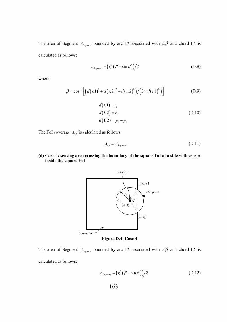
163

The area of Segment SegmentA bounded by arc �1 2 associated with β∠ and chord 1 2 is

calculated as follows:

( )( )2 sin 2Segment sA r β β= − (D.8)

where

( ) ( ) ( )( ) ( )( )2 2 2 21cos ,1 , 2 1, 2 2 ,1d i d i d d iβ − = + − ×

(D.9)

( )( )( ) 2 1

,1

, 2

1, 2

s

s

d i r

d i r

d y y

=

=

= −

(D.10)


,c i SegmentA A= (D.11)

(d) Case 4: sensing area crossing the boundary of the square FoI at a side with sensor

inside the square FoI

Figure D.4: Case 4

The area of Segment SegmentA bounded by arc �1 2 associated with β∠ and chord 1 2 is

calculated as follows:

( )( )2sin 2Segment sA r β β= − (D.12)

,c iA

sr

Square FoI

( )1 1,x y

( )2 2,x y

( ),i ix y

β

Segment

Sensor i

164

where

( ) ( ) ( )( ) ( )( )2 2 2 21cos ,1 , 2 1, 2 2 ,1d i d i d d iβ − = + − ×

(D.13)

( )( )( ) 2 1

,1

, 2

1, 2

s

s

d i r

d i r

d y y

=

=

= −

(D.14)


2

,c i s SegmentA r Aπ= − (D.15)

165

Reference

[1] Wolpert, D.H., Tumer, K.: An introduction to Collective Intelligence. Technical

Report, NASA ARC-IC-99-63, NASA Ames Research Center, (1999)

[2] Bieniawski, S.R.: Distributed Optimization and Flight Control Using Collectives.

PhD Dissertation, Stanford University, CA, USA, (2005)

[3] Wolpert, D.H.: Information Theory ― The Bridge Connecting Bounded Rational

Game Theory and Statistical Physics. Complex Engineered Systems, Braha, D.

Minai, A.A., Bar-Yam Y. (Eds.), Springer (2006), pp. 262-290

[4] Wolpert, D.H., Strauss, C.M.E., Rajnarayan, D.: Advances in Distributed

Optimization using Probability Collectives, Advances in Complex Systems, 9(4), pp.

383-436, (2006)

[5] Basar, T., Olsder, G.J.: Dynamic Non-Cooperative Game Theory. Academic Press,

London/New York, (1995)

[6] Kulkarni A.J., Tai, K.: Solving Constrained Optimization Problems Using

Probability Collectives and a Penalty Function Approach. International Journal of

Computational Intelligence and Applications, 10(4), pp. 445-470, (2011)

[7] Kulkarni A.J., Tai, K.: A Probability Collectives Approach with a Feasibility-based

Rule for Constrained Optimization. Applied Computational Intelligence and Soft

Computing, Vol. 2011, Article ID 980216

[8] Kulkarni A.J., Tai, K.: Solving Sensor Network Coverage Problems Using a

Constrained Probability Collectives Approach. Applied Soft Computing

(Submitted)

[9] Haddin, G.: The Tragedy of Commons. Science, 162, pp. 1243-1248, (1968)

[10] Vasirani, M. Ossowski, S.: Collective-Based Multiagent Coordination: A Case

Study. LNAI 4995, pp. 240–253, (2008)

[11] Bieniawski, S.R., Kroo, I.M., Wolpert, D.H. Discrete, Continuous, and Constrained

Optimization Using Collectives. In: 10th AIAA/ISSMO Multidisciplinary Analysis

and Optimization Conference, 5, pp. 3079-3087, (2004)

[12] Wolpert, D.H., Antoine, N.E., Bieniawski, S.R., Kroo, I.R.: Fleet Assignment Using

Collective Intelligence. In: Proceedings of the 42nd AIAA Aerospace Science

Meeting Exhibit, (2004)

166

[13] Sislak, D., Volf, P., Pechoucek, M., Suri, N.: Automated Conflict Resolution

Utilizing Probability Collectives Optimizer. IEEE Transactions on Systems, Man

and Cybernetics: Applications and Reviews, 41(3), pp. 365-375, (2011)

[14] Bhadra, S., Shakkotai, S., Gupta, P.: Min-cost selfish multicast with network coding.

IEEE Transactions on information Theory, 52(11), pp. 5077-5087, (2006)

[15] Xi, Y., Yeh, E., M.: Distributed algorithms for minimum cost multicast with network

coding in wireless networks. In: Proceedings of 4th International Symposium on

Modeling and Optimization in Mobile, Ad Hoc and Wireless Networks, (2006)

[16] Yuan, J., Li, Z., Yu,W., Li, B.: A cross-layer optimization framework for multicast

in multi-hop wireless networks. In: First International Conference on Wireless

Internet, pp. 47-54, (2005)

[17] Chatterjee, M., Sas, S., K., Turgut, D.: An on-demand weighted clustering algorithm

(WCA) for ad hoc networks,. In: Proceedings of 43rd IEEE Global

Telecommunications Conference, pp. 1697-1701, (2000)

[18] Amerimehr, M.H., Khalaj, B.K., Crespo, P.M.: A Distributed Cross-Layer

OptimizationMethod for Multicast in Interference-Limited Multihop Wireless

Networks. Journal onWireless Communications and Networking, Article ID 702036,

(2008)

[19] Mohammad, H.A., Babak, H.K.: A Distributed Probability Collectives Optimization

Method for Multicast in CDMA Wireless Data Networks. In: Proceedings of 4th

IEEE Internatilonal Symposium on Wireless Communication Systems, art. No.

4392414, pp. 617-621, (2007)

[20] Ryder, G.S., Ross, K.G.: A probability collectives approach to weighted clustering

algorithms for ad hoc networks. In: Proceedings of Third IASTED International

Conference on Communications and Computer Networks, pp. 94-99, (2005)

[21] Autry, B.: University Course Timetabling with Probability Collectives. Master’s

Thesis, Naval Postgraduate School Montery, CA, USA, (2008)

[22] Huang, C.F., Bieniawski, S., Wolpert, D., Strauss, C.E.M.A Comparative Study of

Probability Collectives Based Multiagent Systems and Genetic Algorithms. In:

Proceedings of the Conference on Genetic and Evolutionary Computation, pp. 751 –

752, (2005)

167

[23] Carter, A., Ragsdale C.T.: Scheduling Pre-Printed Newspaper Advertising Inserts

Using Genetic Algorithms. Omega, 30(6), pp. 415–421, (2002)

[24] Tang, L., Liu, J., Rong, A., Yang, Z.: A Multiple Traveling Salesman Problem

Model for Hot Rolling Scheduling in Shangai Baoshan Iron & Steel Complex.

European Journal of Operational Research, 124(2), pp. 267–82, (2000).

[25] Lenstra, J.K., Rinnooy K. AHG.: Some Simple Applications of the Traveling

Salesman Problem. Operational Research Quarterly, 26, pp. 717–33, (1975)

[26] Lin, S.: Computer Solutions of the Traveling Salesman Problem. Bell Systems

Technical Journal, 44(10), pp. 2245-2269, (1965)

[27] Christofides, N., Eilon, S.: An Algorithm for the Vehicle Dispatching Problem.

Operations Research Quarterly, 20, pp. 309-318, (1969)

[28] Savelsbergh, M.W.P.: The General Pickup and Delivery Problem. Transactions of

Science, 29, pp.17-29, (1995).

[29] Svestka, J.A, Huckfeldt, V.E.,: Computational Experience with an M-Salesman

Traveling Salesman Algorithm. Management Science, 19, pp. 790-799, (1973)

[30] Saleh, H.A., Chelouah, R.: The Design of the Global Navigation Satellite System

Surveying Networks Using Genetic Algorithms. Engineering Application of

Artificial Intelligence, 17, pp. 111-122, (2004)

[31] Calvo, R.W., Cordone, R.: A Heuristic Approach to the Overnight Security Service

Problem. Computers and Operations Research, 30, pp.1269–1287, (2003).

[32] Liu, J., Xue, S., Liu, Z., Xu, D.: An improved energy landscape paving algorithm for

the problem of packing circles into a larger containing circle. Computers &

Industrial Engineering, 57(3), pp. 1144-1149, (2009)

[33] Castillo, I., Kampas, F. J., Pinter, J. D.: Solving Circle Packing Problems by Global

Optimization: Numerical Results and Industrial Applications. European Journal of

Operational Research, 191(3), pp. 786-802, (2008)

[34] Xu, X., Sahni, S., Rao, N.S.V.: Minimum-cost Sensor Coverage of Planar Regions.

In: Proceedings of 11th International Conference on Information Fusion, art. no.

4632209, (2008)

[35] Wang, G., Cao, G., La porta T.F.: Movement-Assisted Sensor Deployment. IEEE

Transactions on Mobile Computing, 5 (6), pp. 640-652, (2006)

168

[36] Chakrabarty, K., Iyengar, S.S., Qi, H., Cho, E.: Coding Theory for Target Location

in Distributed Sensor Networks. In: proceedings of IEEE International Conference

on Information Technology: Coding and Computing, pp. 130-134, (2001)

[37] Chakrabarty K., Iyengar, S.S., Qi, H., Cho, E.: Grid Coverage for Surveillance and

Target Location in Distributed Sensor Networks. IEEE Transactions on Computers,

51 (12), pp. 1448-1453, (2002)

[38] Yick, J., Mukherjee, B., Ghosal, D.: Wireless Sensor Network Survey. Computer

Networks. 52(12), pp. 2292-2330, (2008)

[39] Castillo-Effen, M., Quintela, D.H., Jordan, R., Westhoff, W., Moreno, W.: Wireless

sensor networks for flash-flood alerting. In: Proceedings of 5th IEEE International

Caracas Conference on Devices, Circuits, and Systems, Dominican Republic, pp,

142-146, (2004)

[40] Gao, T., Greenspan, D., Welsh, M., Juang, R.R., Alm, A.: Vital signs monitoring and

patient tracking over a wireless network. In: Proceedings of 27th IEEE EMBS

Annual International Conference, pp.102-105, (2005)

[41] Lorincz, K., Malan, D., Fulford-Jones, T.R.F., Nawoj, A., Clavel, A., Shnayder, V.,

Mainland, G., Welsh, M., Moulton, S.: Sensor networks for emergency response:

challenges and opportunities. IEEE Pervasive Computing, 3(4), pp.16-23, (2004).

[42] Wener-Allen, G., Lorincz, K., Ruiz, M., Marcillo, O., Johnson, J., Lees, J., Walsh,

M.: Deploying a wireless sensor network on an active volcano. IEEE Internet

Computing, 10(2), pp. 18-25, (2006)

[43] Zou Y, Chakrabarty, K.: Sensor Deployment and Target Localization Based on

Virtual Forces. In: Proceedings of the IEEE INFOCOM 2003, pp. 1293-1303

[44] Lee. J., Jayasuriya, S.: Deployment of Mobile Sensor Networks with Discontinuous

Dynamics. In: Proceedings of International Federantion of Automatic Control,

pp.10409-10414, (2008)

[45] Gage. D.W.: Command Control for many-robot Systems. Inmanned Systems

Magazine, 10(4), pp. 28-34, (1992)

[46] Sycara, K., Pannu, A., Williamson, M., Zeng, D., Decker, K..: Distributed Intelligent

Agents. IEEE Expert: Intelligent Systems and Their Applications, 11(6), pp. 36-46,

(1996)

169

[47] Maes, P.: Agents that Reduce Work and Information Overload. Communications of

ACM Archives, 37(7), pp.30-40, (1994)

[48] Etzioni, O., Weld, D.: A Softbot-based Interface to the Internet. Communications of

ACM Archives, 37(7), pp.72-79, (1994)

[49] Artfiles.art.com/images/-/David-Dennis/Leaf-Cutting-Ants-Photographic-Print-

C12816629.jpeg (Last Accessed: July 08, 2011)

[50] www.canada-photos.com/data/media/12/busy-honey-bees_1712.jpg (Last Accessed:

July 08, 2011)

[51] Seredynski, F.: Distributed Scheduling Using Simple Learning Machines. European

Journal of Operational Research, 107, pp. 401-413, (1998)

[52] Kim, K., Paulson, B.C.: Multi-Agent Distributed Coordination of Project Schedule

Changes. Computer-Aided Civil and Infrastructure Engineering, 18, 412-425 (2003)

[53] Batista, B.M., Moreno Perez, J.A., Moreno Vega, J.M.: Nature-inspired

Decentralized Cooperative Metaheuristic Strategies for Logistic Problems. In:

Proceedings of European Symposium on Nature-inspired Smart Information

Systems, (2006)

[54] Durfee, E.H., Lesser, V.R., Corkill, D.D.: Trends in Cooperative Distributed

Problem Solving. IEEE Transactions on Knowledge and Data Engineering. 1(1), pp.

63-83, (1989)

[55] Waldock, A., Nicholson, D.: Cooperative Decision Strategies Applied to a

Distributed Sensor Network. In Proceedings of 2nd SEAS DTC Technical

Conference - Edinburgh (2007)

[56] Chandler, P., Rasumussen, S., Pachter, M.: UAV Cooperative Path-planning. In:

Proceedings of AIAA Guidance, Navigation, and Control Conf. Paper. No. 4370,

(2000)

[57] Sislak, D., Volf, P., Komenda, A., Samek, J., Pechoucek, M.: Agent-based Multi-

layer Collision Avoidance to Unmanned Aerial Vehicles. In: Proceedings of

International Conference on Integration of Knowledge Intensive Multi-Agent

Systems, Art. No. 4227576, pp. 365-370, (2007)

170

[58] Krozel, J., Peters, M., Bilimoria, K.: A Decentralized Control Strategy for

Distributed Air/Ground Traffic Separation. In: Proceedings of AIAA Guidance,

Navigation and Control Conference and Exhibit, Paper, No. 4062, (2000)

[59] Zengin, U., Dogan, A.: Probabilistic Trajectory Planning for UAVs in Dynamic

Environments. In: Proceedings of AIAA 3rd "Unmanned-Unlimited" Technical

Conference, Workshop, and Exhibit 2, Paper, No. 6528, (2004)

[60] Anderson, M.R., Robbins, A.C.: Formation Flight as A Cooperative Game. In:

Proceedings of AIAA Guidance, Navigation, and Control Conference, pp. 244-251,

(1998)

[61] Chang, D.E., Shadden, Marsden J. E., Olfati-Saber, R.: Collision Avoidance for

Multiple Agent Systems. In: Proc. of 42nd IEEE Conference on Decision and

Control, pp. 539-543, (2003)

[62] Sigurd, K., How, J.: UAV Trajectory DesignUsing Total Field Collision Avoidance.

In: Proceedings of AIAA Guidance, Navigation, and Control Conference, Paper No.

5728, (2003)

[63] Lesser, V.R., Erman, L.D.: Distributed Interpretation: A model and Experiment.

IEEE Transactions on Computers. C-29(12), pp. 1144-1163, (1980)

[64] Ogston, E., Zeman, A., Prokopenko M., James G.: Clustering Distributed Energy

Resources for Large-Scale Demand Management. 9(11), pp. 97 – 108, (2007)

[65] Wolpert, D.H., Tumer, K., Frank, J.: Collective Intelligence to Route Internet

Traffic. Advances in Neural Information Processing Systems-11, MIT Press, pp.

952-958, (1999)

[66] Chanyagom, P., Szu, H.,H., Wang, H.: Collective Behavior Implementation in

Powerline Surveillance Sensor Network. In: Proceedings of International Joint

Conference on Neural Networks, pp. 1735-1739, (2005)

[67] Rabbat, M., Nowak, R.: Distributed Optimization in Sensor Networks. In: Proc. of

Third International Symposium on Information Processing in Sensor Networks,

pp. 20-27, (2004)

[68] Petcu, A., Artificial Intelligence Laboratory. EPFL, Switzerland.

http://liawww.epfl.ch/Research/dcr/ (Last Accessed: July 08, 2011)

171

[69] Campbell, M., Cagan, J., Kotovsky, K.: A-Design: An Agent-Based Approach to

Conceptual Design in a Dynamic Environment. Research in Engineering Design, 11,

pp.172–192, (1999)

[70] http://www.det.csiro.au/science/de_s/index.htm (Last Accessed: July 08, 2011)

[71] http://www.nrel.gov/learning/eds_distributed_energy.html (Last Accessed: July 08,

2011)

[72] Visentin, G.,Winnendael, M.,V., Putz, P.: Advanced Mechatronics in ESA Space

Robotics Developments. In: Proceedings of the IEEE/RSJ International Conference

on Intelligent Robots and Systems, 2, pp. 1261–1266, (2001)

[73] Casper, J., Murphy, R.R., Micire, M.: Issues in Intelligent Robots for Search And

Rescue. In: Proceedings of the SPIE Unmanned Ground Vehicle Technology 2.

4024, pp. 292–302, (2000)

[74] Ayers, J., Zavracky, P., McGruer, N., Massa, D.P., Vorus, W.S., Mukherjee, R.,

Currie, S.N.: A Modular Behavioral Based Architecture for Biomimetic

Autonomous Underwater Robots. In: Proceedings of the Autonomous Vehicles in

Mine Countermeasures Symposium, Naval Postgraduate School: Monterey,

California, USA, (1998)

[75] Stengel, R., F.: Intelligent Failure-Tolerant Control. IEEE Control Systems

Magazine, 11(4):14–23, (1991)

[76] Mondada, F., Pettinaro, G., C., Guignard, A., Kwee, I.,W., Floreano, D.,

Deneubourg, J., Nolfi, S., Gambardella, L., M., Dorigo, M.: Swarm-Bot: A New

Distributed Robotic Concept. Autonomous Robots, 17, pp. 193–221, (2004)

[77] Kamimura, A., Murata, S., Yoshida, E., Kurokawa, H., Tomita, K., and Kokaji, S.:

Self-reconfigurable Modular Robot Experiments on Reconfiguration and

Locomotion. In: Proceedings of the 2001 IEEE/RSJ International Conference on

Intelligent Robots and Systems IROS2001, 1, pp. 606–612, (2001)

[78] Duff, D., Yim, M., and Roufas, K.: Evolution of PolyBot: A modular Reconfigurable

Robot. In: Proceedings of COE/Super Mechano-Systems Workshop, Tokyo, Japan,

(2001)

172

[79] Rathinam, S., Sengupta, R., Darbha S.: A Resource Allocation Algorithm for

Multivehicle Systems with Nonholonomic Constraints. IEEE Transactions on

Automation Science and Engineering, 4(1), pp. 98-104, (2007)

[80] Zengin, U., Dogan, A.: Probabilistic Trajectory Planning for UAVs in Dynamic

Environments. In: Proceedings of AIAA 3rd "Unmanned-Unlimited" Technical

Conference, Workshop, and Exhibit 2, Paper, No. 6528, (2004)

[81] Garagic, D., Mehra, R.K.: Distributed,Decentralized Optimization for Cooperative

Control of Multi-Agent Swarm-like Systems. Final Report, NAVY Phase 1 STTR,

Contract No. N00014-04-M-0289, (2005)

[82] Kulkarni, A.J., Tai, K.: Probability Collectives for Decentralized, Distributed

Optimization: A Collective Intelligence Approach. In: Proceedings of the IEEE

International Conference on Systems, Man, and Cybernetics, pp. 1271-1275, (2008)

[83] Kulkarni, A.J. Tai, K.: Probability Collectives: A Decentralized, Distributed

Optimization for Multi-Agent Systems. Applications of Soft Computing, Mehnen, J.,

Koeppen, M., Saad, A., Tiwari, A. (Eds.), Springer (2009), pp. 441-450

[84] Kulkarni, A.J., Tai, K.: Probability Collectives: A Multi-Agent Approach for

Solving Combinatorial Optimization Problems. Applied Soft Computing, 10(3), pp.

759-771, (2010)

[85] Kulkarni A.J., Tai, K.: Probability Collectives: A Distributed Optimization

Approach for Constrained Problems. In: Proceedings of IEEE World Congress on

Computational Intelligence, pp. 3844-3851, (2010)

[86] Huang, C.F., Chang, B.R.: Probability Collectives Multi-agent Systems: A Study of

Robustness in Search. LNAI 6422, Part II, pp. 334-343, (2010)

[87] Zhang, X.P, Yu, W.H., Liang, J.J., Liu, B.: Entropy Regularization for Coordinated

Target Assignment. In: Proceedings of 3rd IEEE Conference on Computer Science

and Information Technology, pp. 165-169, (2010)

[88] Smyrnakis, M., Leslie, D.S.: Sequentially Updated Probability Collectives. In:

Proceedings of 48th IEEE Conference on Decision and Control and 28th Chinese

Control Conference, pp. 5774-5779, (2009)

[89] Luo, D.L., Shen, C.L., Wang, B., Wu, W.H.: Air Combat Decision-Making for

Cooperative Multiple Target Attack Using Heuristic Adaptive Genetic Algorithm.

173

In: Proceedings of IEEE International Conference on Machine Learning and

Cybernetics IEEE Press, pp. 473-478, (2005)

[90] Luo, D.L., Duan, H.B. Wu, S.X., Li, M.Q.: Research on Air Combat Decision-

making for Cooperative Multiple Target Attack Using Heuristic Ant Colony

Algorithm. Acta Aeronautica et Astronautica Sinica, 27(6), pp. 1166- 1170, (2006)

[91] Luo, D.L., Yang, Z., Duan, H.B., Wu, Z.G., Shen, C.L.: Heuristic Particle Swarm

Optimization Algorithm for Air Combat Decision-Making on CMTA. Transactions

of Nanjing University of Aeronautics & Astronautics, 23(1), pp. 20-26, (2006)

[92] Modi, P., Shen, W., Tambe, M., Yokoo, M.: Adopt: Asynchrous Distributed

Constraint Optimization with Quality Guarantees. Artificial Intelligence, 161, pp.

149-180, (2005)

[93] Goldberg, D.E., Samtani, M.P.: Engineering optimization via genetic algorithm. In:

Proceedings of 9th Conference on Electronic Computation, pp. 471-484, (1986)

[94] Ghasemi, M.R., Hinton, E., Wood, R.D.: Optimization of trusses using genetic

algorithms for discrete and continuous variables. Engineering Computations, 16(3),

pp. 272-301, (1999)

[95] Moh, J., Chiang, D.:Improved Simulated Annealing Search for Structural

Optimization. AIAA Journal, 38(10), pp. 1965-1973, (2000)

[96] Arora, J.S.: Introduction to Optimum Design. Elsevier Academic Press, (2004)

[97] Vanderplaat, G.N.: Numerical Optimization Techniques for Engineering Design.

Mcgraw-Hill, (1984)

[98] Shoham, Y., Powers, R., Grenager, T.: Multi-agent reinforcement learning: A critical

survey. Available online:

www.cc.gatech.edu/~isbell/reading/papers/MALearning.pdf (Last Accessed on: July

23, 2011)

[99] Busoniu, L., Babuska, L., Schutter, B.: A Comprehensive Survey of Multiagent

Reinforcement Learning. IEEE Transactions on Systems, Man, and Cybernetics—

Part C: Applications and Reviews, 38(2), pp. 156-172, (2008)

[100] Bowling, M., Veloso, M.: Multiagent learning using a variable learning rate.

Artificial Intelligence, 136(2), pp. 215–250, (2002)

174

[101] Bowling, M., Veloso, M.: Rational and convergent learning in stochastic games. In:

Proceedings of 17th International Conference on Artificial Intelligence, pp. 1021–

1026, (2001)

[102] Sindhwani, V., Keerthi, S.S., Chapelle, O.: Deterministic Annealing for Semi-

supervised Kernel Machines. In: Proceedings of the 23rd International Conference

on Machine Learning, (2006)

[103] Rao, A.V., Miller, D.J., Rose, K., Gersho,A.: A Deterministic Annealing Approach

for Parsimonious Design of Piecewise Regression Models. IEEE Transactions on

Patternt Analysis and Machine Intelligence, 21(2), (1999)

[104] Rao, A.V., Miller, D.J., Rose, K., Gersho,A.: Mixture of Experts Regression

Modeling by Deterministic Annealing. IEEE Transactions on Signal Processing,

45(11), (1997)

[105] Czabanski, R.: Deterministic Annealing Integrated with Intensive Learning in

Neuro-fuzzy Systems. LNAI 4029, pp. 220-229, (2006)

[106] hyperphysics.phy-astr.gsu.edu/hbase/thermo/helmholtz.html. (Last accessed on: July

30, 2010)

[107] Cheng, C.T., Wang W.C., Xu, D.M., Chau K.W.: Optimizing Hydropower Reservoir

Operation Using Hybrid Genetic Algorithm and Chaos. Water Resource

Management, 22, pp. 895–909, (2008)

[108] Blumenthal, H. J., Parker, G.B.: Benchmarking Punctuated Anytime Learning for

Evolving a Multi-Agent Team's Binary Controllers. In: Proceedings of World

Automation Congress, pp. 1-8, (2006)

[109] Roger, Tan, L.S., Srinivas, M., Rangaiah, G.P.: Global Optimization of Benchmark

and Phase Equilibrium Problems using Differential Evolution. Available online:

http://www.ies.org.sg/journal/current/v46/v462_3.pdf

[110] Bouvry, P., Arbab F., Seredynski, F.: Distributed Evolutionary Optimization, in

Manifold: Rosenbrock's function case study. Information Sciences, 122, pp. 141-

159, (2000)

[111] Durbin, R, Willshaw, D.J.: An Analogue Approach to the Traveling Salesman

Problem Using an Elastic Net Method. Nature, 326, pp. 689-691, (1987)

175

[112] Papadimitriou C. H.: The Euclidean Traveling Salesman Problem is NP-Complete.

Theoretical Computer Science, 4, pp. 237-244, (1977)

[113] Bektas, T.: The Multiple Traveling Salesman Problem: An Overview of

Formulations and Solution Procedures. Omega, 34, pp. 209 – 219, (2006)

[114] Golden, B, Levy L, Dahl R. Two Generalizations of the Traveling Salesman

Problem. Omega, 9(4), pp. 439–441, (1981)

[115] Lawler, E., Lenstra, J., Rinnooy, K. AHG, Shmoys, D.: The Traveling Salesman

Problem. Chichester: Wiley, (1985)

[116] Laporte, G.: The Traveling Salesman Problem: An Overview of Exact and

Approximate Algorithms. European Journal of Operational Research, 59, pp. 231–

247 (1992)

[117] Gutin, G., Punnen, A.P., editors. Traveling Salesman Problem and its Variations.

Dordrecht: Kluwer Academic Publishers, (2002)

[118] Potvin, J.Y.: A Review of Bio-Inspired Algorithms for Vehicle Routing. Studies in

Computational Intelligence, 161, pp.1-34, (2009)

[119] Renaud, J., Laporte, G., Boctor F. F.: A Tabu Search Heuristic for the Multi-Depot

Vehicle Routing Problem. Computers & Operations Research 23(3): 229-235,

(1996)

[120] Cassidy, P. J., Bennett, H. S.: TRAMP - A Multi-depot Vehicle Scheduling System.

Operational Research Quarterly. 23, 151-163, (1972)

[121] Pooley, J.: Integrated Production and Distribution Facility Planning at Ault Foods.

Interfaces, 24, pp. 113-121, (1994)

[122] Ball, M.O., Golden, B.L., Assad, A.A., Bodin, L.D.: Planning for Truck Fleet Size in

the Presence of A Common-Carrier Option. Decision Science, 14, pp. 103-120,

(1983)

[123] Bell, W.J., Dalberto, L.M., Fisher, M.L., Greenfield, A.J., Jaikumar, R., Kedia,

P., Mack, R.G., Prutzman, P.J.: Improving the Distribution of Industrial Gases with

an On-Line Computerized Routing and Scheduling Optimizer. Interfaces, 13 (6), pp.

4-23, (1983)

[124] Ghaziri, H., Osman, I.H.: Self-Organizing Feature Maps for the Vehicle Routing

Problem with Backhauls. Journal of Scheduling, 9 (2), pp. 97-114, (2006)

176

[125] Taillard, E.D., Laporte, G., Gendreau, M.: Vehicle Routing with Multiple Use of

Vehicles. Journal of the Operational Research Society, 47, 1065–1070, (1996)

[126] Crevier, B., Cordeau, J.-F., Laporte, G.: The Multi-Depot Vehicle Routing Problem

with Inter-Depot Routes. European Journal of Operational Research, 176 (2), pp.

756-773, (2007)

[127] Chen, A.-L., Yang, G.-K., Wu, Z.-M.: Hybrid Discrete Particle Swarm Optimization

Algorithm for Capacitated Vehicle Routing Problem. Journal of Zhejiang University

Science, 7 (4), pp. 607-614, (2006)

[128] Bellmore, M., Hong, S.: Transformation of Multisalesmen Problem to the Standard

Traveling Salesman Problem. Journal of the Association Computer Machinery, 21,

pp, 500-504, (1974)

[129] Wacholder, E., Han, J., Mann, R.C.: An Extension of the Hopfield-Tank Model for

Solution of The Multiple Traveling Salesmen Problem. In: Proceedings of the Neural

Networks, 2, pp. 305-324, (1988)

[130] Somhom, S., Modares, A., Enkawa T.: Competition-Based Neural Network for the

Multiple Travelling Salesmen Problem with Minmax Objective. Computers &

Operations Research, 26, pp. 395-407, (1999)

[131] Pan. J., Wang, D.: An Ant Colony Optimization Algorithm for Multiple Travelling

Salesman Problem. In: Proceedings of First International Conference on Innovative

Computing, Information and Control, pp. 210-213, (2006)

[132] Christofides, N., Mingozzi, A., Toth, P.: Exact Algorithms for the Vehicle Routing

Problem, Based On Spanning Tree And Shortest Path Relaxations. Mathematical

Programming 20, pp. 255-282, (1981)

[133] Laporte, G., Nobert, Y.: A Cutting Planes Algorithms for the M-Salesmen Problem.

Operations Research Quarterly, 31, pp. 1017-1023, (1980)

[134] Zhu, Q., Qian, L., Li, Y., Zhu, S. An Improved Particle Swarm Optimization

Algorithm for Vehicle Routing Problem with Time Windows. In.: Proceedings of the

IEEE Congress on Evolutionary Computation, pp. 1386-1390, (2006)

[135] Shima, T., Rasmussen S., Gross, D.: Assigning Micro UAVs to Task Tours in an

Urban Terrain. IEEE Transactions on Control Systems Technology, 15, (4), pp. 601-

612, (2007)

177

[136] Rathinam, S., Sengupta, R., Darbha S.: A Resource Allocation Algorithm for

Multivehicle Systems with Nonholonomic Constraints. IEEE Transactions on

Automation Science and Engineering. 4(1), pp. 98-104, (2007)

[137] Reimann, M., Ulrich, H.: Comparing Backhauling Strategies in Vehicle Routing

Using Ant Colony Optimization. Central European Journal of Operations

Research, 14 (2), pp. 105-123, (2006)

[138] Shetty, V.K., Sudit, M., Nagi, R.: Priority-based Assignment and Routing of A Fleet

of Unmanned Combat Aerial Vehicles. Computers & Operations Research, 35, pp.

1813 – 1828, (2008)

[139] Gambardella, L.M., Taillard, E.D., Agazzi, G.: MACS-VRPTW: A Multiple Ant

Colony System for Vehicle Routing Problems with Time Windows. New ideas in

optimization, pp. 63-76, (1999)

[140] Ombuki-Berman, B., Hanshar, F.T., Using Genetic Algorithms for Multi-depot

Vehicle Routing. Studies in Computational Intelligence, 161, pp. 77-99, (2009)

[141] Thangiah, S.R., Salhi, S.: Genetic Clustering: An Adaptive Heuristic for the

Multidepot Vehicle Routing Pproblem. Applied Artificial Intelligence, 15, pp. 361–

383, (2001)

[142] Vakhutinsky, I., A., Golden, L., B.: Solving Vehicle Routing Problems Using Elastic

Net. In: Proceedings of IEEE International Conference on Neural Network, pp.

4535-4540, (1994)

[143] Bullnheimer, B., Hartl, R.F., Strauss, C.: Applying The Ant System to The Vehicle

Routing Problem. Metaheuristics: Advances and trends in local search paradigms for

optimization, Dordrecht: Kluwer, pp. 285-296, (1999)

[144] Goldberg, D.E.: Alleles, Loci and The Traveling Salesman Problem. In: Proceedings

of the First International Conference on Genetic Algorithms and Their Applications,

pp. 154-159, (1985)

[145] Hopfield J. J. Tank D. W.: Neural Computation of Decisions in Optimization

Problems. Biology in Cybernetics, 5, pp. 141-152, (1985)

[146] Wilson GV, Pawley GS.: On The Stability of The Travelling Salesman Problem

Algorithm of Hopfield and Tank. Biology in Cybernetics, 58, pp. 63-70, (1988)

178

[147] Cordeau, J.F., Desaulniers, G., Desrosiers, J., Solomon, M.M., Soumis, F.: VRP with

Time Windows. In: Toth P, Vigo D, editors. The vehicle routing problem. SIAM, pp.

157–193, (2002)

[148] Eisenstein, D.D., Iyer, A.V.: Garbage collection in Chicago: A Dynamic Scheduling

Model. Management Science, 43(7), pp. 922–933, (1997)

[149] Tung, D.V., Pinnoi. A.: Vehicle Routing-Scheduling for Waste Collection in Hanoi.

European Journal of Operational Research, 125, pp. 449–468, (2000)

[150] Klesh, A.T., Kabamba, P.T., Girard, A.R.: Path Planning for Cooperative Time-

Optimal Information Collection. In: Proceedings of American Control Conference,

pp. 1991-1996, (2008)

[151] Yadlapalli, S., Malik, W.A., Rathinam, S. Darbha, S.: A Lagrangian-Based

Algorithm for a Combinatorial Motion Planning Problem. In: Proceedings of 46th

IEEE Conference on Decision and Control, USA, pp. 5979-5984, (2007)

[152] Dubins, L.: On Curves of Minimal Length With A Constraint on Average Curvature

and with Prescribed Initial and Terminal Position. American Journal of Mathematics,

79, pp. 497–516, (1957)

[153] Concorde, Georgia Inst. Technol., Atlanta, Software package, Ver 03.12.19, (2006).

Available Online: http://www.tsp.gatech.edu/concorde/index.html (Last Accessed:

July 23, 2011)

[154] Miliotis, P.: Using Cutting Planes to Solve the Symmetric Traveling Salesman

Problem. Mathematical Programming, 15, pp. 177-188, (1978)

[155] Coello Coello, C.A.: Use of Self-adaptive Penalty Approach for Engineering

Optimization Problems. Computers in Industry, 41, pp. 113-127, (2000)

[156] Runarsson, T.P., Yao, X.: Stochastic Ranking for Constrained Evolutionary

Optimization. IEEE Transactions on Evolutionary Computation, 4(3), pp. 284-294,

(2000)

[157] Farmani, R., Wright, J.A.: Self-Adaptive Fitness Formulation for Constrained

Optimization. IEEE Transactions on Evolutionary Computation, 7(5), pp. 445-455,

(2003)

[158] Homaifar, A., Qi, C.X., Lai, S.H.: Constrained Optimization via Genetic Algorithms.

Simulation, 62(4), pp. 242-254, (1994)

179

[159] Deb, K.: An Efficient Constraint Handling Method for Genetic Algorithms.

Computer Methods in Applied Mechanics in Engineering, 186, pp. 311-338, (2000)

[160] He, Q., Wang, L.: A Hybrid Particle Swarm Optimization with a Feasibility-based

Rule for Constrained Optimization. Applied Mathematics and Computation, 186, pp.

1407-1422, (2007)

[161] Michalewicz, Z., Janikow, C.Z.: Handling Constraints in Genetic Algorithms. In:

Proceedings of International Conference on Genetic Algorithms, 4, pp. 151-157,

(1991)

[162] Michalewicz, Z.: Numerical Optimization: Handling Linear Constraints. Handbook

of Evolutionary Computation, IOP Publishing, G9.1, (1997)

[163] Hu, X., Eberhart, R.: Solving Constrained Nonlinear Optimization Problems with

Particle Swarm Optimization. In: Proceedings of the 6th World Multi-conference on

Systemics, Cybernetics and Informatics, (2002)

[164] Koziel, S., Michalewicz, Z.: Evolutionary Algorithms, Homomorphous Mapping,

and Constrained Parameter Optimization. Evolutionary Computation, 7(1), pp. 19-

44, (1999)

[165] Coello Coello, C.A., Becerra, R.L.: Efficient Evolutionary Optimization Through the

Use of A Cultural Algorithm. Engineering Optimization, 36(2), pp. 219-236, (2004)

[166] Becerra, R.L., Coello Coello, C.A.: Cultured Differential Evolution for Constrained

Optimization. Computer Methods in Applied Mechanics and Engineering, 195, pp.

4303-4322, (2006)

[167] Chootinan, P., Chen, A.: Constraint Handling in Genetic Algorithms Using a

Gradient-based Repair Method. Computers and Operations Research, 33, pp. 2263-

2281, (2006)

[168] Zahara, E., Hu, C.H.: Solving Constrained Optimization Problems with Hybrrid

Particle Swarm Optimization. Engineering Optimization, 40(11), pp. 1031-1049,

(2008)

[169] Dong, Y., Tang, J., Xu, B., Wang, D.: An Application of Swarm Optimization to

Nonlinear Programming. Computers and Mathematics with Applications, 49, pp.

1655-1668, (2005)

180

[170] Hedar, A.R., Fukushima, M.: Derivative-Free Simulated Annealing Method for

Constrained Continuous Globale Optimization. Journal of Global Optimization, 35,

pp. 521-549, (2006)

[171] Coello Coello, C.A., Montes, E.M.: Constraint-handling in Genetic Algorithms

through the Use of Dominance-based Tournament Selection. Advanced Engineering

Informatics, 16, pp. 193-203, (2002)

[172] Ray, T., Tai, K., Seow, K.C.: An Evolutionary Algorithm for Constrained

Optimization. In: Proceedings of the Genetic and Evolutionary Computation

Conference, pp. 771-777, (2000)

[173] Ray, T., Tai, K., Seow, K.C.: Multiobjective Design Optimization by an

Evolutionary Algorithm. Engineering Optimization, 33(4), pp. 399-424, (2001)

[174] Tai, K., Prasad, J.: Target-Matching Test Problem for Multiobjective Topology

Optimization Using Genetic Algorithms. Structural and Multidisciplinary

Optimization, 34(4), pp. 333-345, (2007)

[175] Runarsson, T.P., Yao, X.: Search Biases in Constrained Evolutionary Optimization.

IEEE Transactions on Systems, Man and Cybernetics-Part C: Applications and

Reviews, 35(2), pp. 233-243, (2005)

[176] Himmelblau, D.M.: Applied Nonlinear Programming. Mcgraw-Hill, (1972)

[177] White W.B., Johnson, S.M., Dantzig, G.B.: Chemical Equilibrium in Complex

Mixtures. Chemical Physics, 28(5), pp. 751-755, (1958)

[178] Hock, W., Schittkowski, K.: Test examples for nonlinear programming codes.

Lecture notes in Economics and Mathematical Systems, 187, Berlin, Heidelberg-

New York: Springer, (1981)

[179] Sakthivel, V.P., Bhuvaneswari, R., Subramanian, S.: Design Optimization of Three-

Phase Energy Efficient Induction Motor Using Adaptive bacterial Foraging

Algorithm. Computation and Mathematics in Electrical and Electronic Engineering,

29(3), pp. 699-726, (2010)

[180] Kaveh, A., Talatahari, S.: An Amproved Ant Colony Optimization for Constrained

Engineering Design Problems. Computer Aided Engineering and Software, 27(1),

pp. 155-182, (2010)

181

[181] Bansal, S., Mani, A., Patvardhan, C.: Is Stochastic Ranking Really Better than

Feasibility Rules for Constraint Handling in Evolutionary Algorithms? In

Proceedings of World Congress on Nature and Biologically Inspired Computing, pp.

1564-1567, (2009)

[182] Gao, J., Li, H., Jiao, Y.C.: Modified Differential Evolution for the Integer

Programming Problems. In Proceedings of International Conference on Artificial

Intelligence, pp. 213-219, (2009)

[183] Ping, W., Xuemin, T.: A Hybrid DE-SQP Algorithm with Switching Procedure for

Dynamic Optimization. In Proceedings of Joint 48th IEEE Conference on Decision

and Control and 28th Chinese Control Conference, pp.2254-2259, (2009)

[184] Zhang, D., Deng, A.: An effective hybrid algorithm for the problem of packing

circles into a larger containing circle. Computers & Operations Research, 32, pp.

1941–1951, (2005)

[185] Theodoracatos, V. E., Grimsley, J. L.: The optimal packing of arbitrarily-shaped

polygons using simulated annealing and polynomial-time cooling schedules.

Computer Methods in Applied Mechanics and Engineering, 125, pp. 53-70, (1995)

[186] Garey, M. R,, Johnson D. S.: Computers and intractability: A Guide to the Theory of

NP-completeness. W. H. Freeman & Co. (1979)

[187] Hochbaum, D. S., Maass, W.: Approximation schemes for covering and packing

problems in image processing and VLSI. Journal of the Association for Computing

Machinery, 1(32), pp. 130–136 (1985)

[188] Wang, H., Huang, W., Zhang, Q., Xu, D.: An improved algorithm for the packing of

unequal circles within a larger containing circle. European Journal of Operational

Research, 141, pp. 440–453, (2002)

[189] Szabo, P.G., Markot, M.C., Csendes, T.: Global optimization in geometry - circle

packing into the square. Essays and Surveys in Global Optimization, Audet, P.,

Hansen, P., Savard, G. (Eds.), Kluwer (2005), pp. 233-265

[190] Nurmela, K.J., Ostergard, P.R.J.: Packing up to 50 equal circles in a square. Discrete

& Computational Geometry, 18, pp. 111–120, (1997)

[191] Nurmela, K.J., Ostergard, P.R.J.: More Optimal Packing of Equal Circles in a

Square. Discrete and Computational Geometry, 22, pp. 439-457, (1999)

182

[192] Graham R. L., Lubachevsky, B. D.: Repeated Patterns of Dense Packings of Equal

Disks in a Square. The Electronic Journal of Combinatorics, 3, R16, (1996)

[193] Szabo, P.G., Csendes, T., Casado, L.G., Garcia, I.: Equal circles packing in a square

I - Problem Setting and Bounds for Optimal Solutions. Optimization Theory: Recent

Developments from Matrahaza, Giannessi, F., Pardalos, P., Rapcsak, T. (Eds.),

Kluwer, (2001), pp. 191-206

[194] de Groot, C, Peikert, R. Wurtz, D.: The Optimal Packing of Ten Equal Circles in a

Square, IPS Research Report 90-12, ETH, Zurich, (1990)

[195] Goldberg, M.: The packing of equal circles in a square, Mathematics Magazine, 43,

pp. 24-30, pp. 24-30, (1970)

[196] Mollard, M., Payan, C.: Some Progress in the Packing of Equal Circles in a Square.

Discrete Mathematics, 84, pp. 303-307, (1990)

[197] Schaer, J.: On the Packing of Ten Equal Circles in a Square, Mathematics Magazine,

44, pp. 139–140, (1971)

[198] Schluter, K., Kreispackung in Quadraten, Elemente der Mathematics, 34, pp. 12-14,

(1979)

[199] Valette, G.: A Better Packing of Ten Circles in a Square, Discrete Mathematics, 76,

pp. 57–59, (1989)

[200] Boll, D.W., Donovan, J., Graham, R.L., Lubachevsky, B.D.: Improving Dense

Packings of Equal Disks in a Square. The Electronic Journal of Combinatorics, 7,

R46, (2000)

[201] Lubachevsky, D, Graham, R.L.: Curved hexagonal packing of equal circles in a

circle. Discrete & Computational Geometry, 18, pp. 179–94, (1997)

[202] Szabo, P. G. Specht, E.: Packing up to 200 Equal Circles in a Square. Models and

Algorithms for Global Optimization, Torn, A., Zilinskas, J. (Eds.), pp. 141-156,

(2007)

[203] Mladenovic, N., Plastria, F., Urosevi, D.: Formulation Space Search for Circle

Packing Problems. LNCS, pp. 212-216, (2007)

[204] Mldenovic, N., Plastria, F., Urosevi, D.: Reformulation Descent Applied to Circle

Packing Problems. Computers and Operations Research, 32, pp. 2419–2434, (2005)

183

[205] Huang, W., Chen, M.: Note on: An Improved Algorithm for the Packing of Unequal

Circles within a Larger Containing Circle. Computers and Industrial Engineering,

50(2), pp, 338-344, (2006)

[206] Liu, J., Xu, D., Yao, Y., Zheng, Y.: Energy Landscape Paving Algorithm for Solving

Circles Packing Problem. In: International Conference on Computational

Intelligence and Natural Computing. pp. 107-110, (2009)

[207] Liu, J., Yao,Y., Zheng, Y., Geng, H., Zhou, G.: An Effective Hybrid Algorithm for

the Circles and Spheres Packing Problems. LNCS-5573, pp. 135-144, (2009)

[208] Stoyan, Y.G., Yaskov, G.N.: Mathematical Model and Solution Method of

Optimization Problem of Placement of Rectangles and Circles Taking into Account

Special Constraints. International Transactions in Operational Research 5, pp. 45–

57, (1998)

[209] Stoyan, Y.G., Yaskov, G.N.: A Mathematical Model and a Solution Method for the

Problem of Placing Various-Sized Circles into a Strip. European Journal of

Operational Research, 156, pp. 590–600, (2004)

[210] George, J.A.: Multiple Container Packing: A Case Study of Pipe Packing. Journal of

the Operational Research Society, 47, pp. 1098–1109, (1996)

[211] George, J.A., George, J.M., Lamar, B.W.: Packing Different-sized Circles into a

Rectangular Container. European Journal of Operational Research, 84, pp. 693–712,

(1995)

[212] Hifi, M., M’Hallah, R.: Approximate Algorithms for Constrained Circular Cutting

Problems. Computers and Operations Research, 31, pp. 675–694, (2004)

[213] Wolpert, D.H., Macready, W.G.: No Free Lunch Theorems for Optimization. IEEE

Transactions on Evolutionary Computation, 1(1), pp. 67-82, (1997)

[214] Lazos, L., Poovendran, R.: Stochastic coverage in heterogeneous sensor networks.

ACM Transactions on Sensor Networks, 2 (3), pp. 325-358, (2006)

[215] Meguerdichian, S. Koushanfar, F., Potkonjak, M., Srivastava, M.B.: Coverage

Problems in Wireless Ad-hoc Sensor Networks, In: Proceedings of IEEE

International Conference on Computer Communications, pp. 1380-1387, (2001)

184

[216] Lazos, L., Poovendran, R.: Detection o Mobile Coverage Targets on the Plane and in

Space using Heterogeneous Sensor Networks. Wireless Networks, 15(5), pp. 667-

690, (2009)

[217] Lazos, L., Poovendran, R.: Coverage in Heterogeneous Sensor Networks. In:

Proceedings of International Symposium of Modeling and Optimization in Mobile,

Ad-Hoc and Wireless Networks, pp. 1-10, (2006)

[218] Xing, G., Wang, X., Zhang, Y., Lu, C., Pless R., Gill, C.: Integrated Coverage and

Connectivity Configuration in Wireless Sensor Networks. ACM Transactions on

Sensor Networks, 1(1), pp. 36-72, (2005)

[219] Iyengar, R., Kar, K., Banerjee, S.: Low-coordination Topologies for Redundancy in

Sensor Networks. In Proceedings of 6th ACM Annual International Symposium on

Mobile Ad-Hoc Networking and Computing, pp. 332-342, (2005)

[220] Clouqueur, T., Phipatanasuphorn, V., Ramanathan P., Saluja, K.K.: Sensor

Deployment Strategy for Target Detection. In: Proceedings of 1st ACM International

Workshop on Wireless Sensor Networks and Applications, pp. 42-48, (2002)

[221] Zhao, F., Guibas, L.: Wireless Sensor Networks. Morgan Kaufmann, (2004)

[222] Fortune, S., Du, D., Hwang, F: Voronoi Diagrams and Delaunay Triangulations.

Handbook of Euclidean Geometry and Computers, CRC Press, 1997

[223] Liu, B., Towsley, D.: A Study of the Coverage of Large-scale Sensor Networks. In:

Proceedings of IEEE International Conference on Mobile Ad-Hoc and Sensor

Systems, pp. 475-483, (2004)

[224] Poduri, S., Sukhatme, G. S.: Constrained Coverage for Mobile Sensor Networks, In:

Proceedings of IEEE International Conference on Robotics and Automation, pp.

165–172, (2004)

[225] Marengoni, M., Draper, B.A., Hanson, A., Sitaraman, R.A.: System to Place

Observers on a Polyhedral Terrain in Polynomial Time. Image and Vision

Computing, 18(10), pp. 773-80, (1996)

[226] Kumar, S., Lai, T.H., Arora, A.: Barrier Coverage with Wireless Sensors. In:

Proceedings of 11th Annual International Conference on Mobile Computing and

Networking, pp. 284-298, (2005)

185

[227] Bai, X., Kumar, S., Xuan, D., Yun, Z., Lai, T.H.: In: Proceedings of International

Symposium on Mobile Ad Hoc Networking and Computing. Deploying Wireless

Sensors to Achieve Both Coverage and Connectivity. pp. 131-142, (2006)

[228] Lugar, G.F.: Artificial Intelligence: Structures and Strategies for Complex Problem

Solving, Addison- Wesley, (2005)

[229] Tosserams, S., Kokkolaras, M., Etman, L.F.P., Rooda, J.E.: A Non-hierarchical

Formulation of Analytical Target Cascading. Journal of Mechanical Design, 132(5),

pp. 051002-1-13, (2010)

[230] Cui, G.Y., Tai, K., Wang, B.P.: Topology Optimization for Maximum Natural

Frequency using Simulated Annealing and Morphological Representation. AIAA

Journal, 40(3), pp. 586-589, (2002)

[231] Wang, B.P., Chen, J. L.: Application of Genetic Algorithm for the Support Location

Optimization of Beams. Computers and Structures, 58(4), pp. 797-800, (1996)

[232] Liu, T.I., Oh, C.T.: An Artificial Intelligence Approach for the Design and

Manufacturing of Micro Electro Mechanical Systems. International Journal of

Knowledge-Based and Intelligent Engineering Systems, 9(2), pp. 159-171, (2005)

[233] Liu, T.I., Oh, C.T.: Intelligent Design for Disassembly. International Journal of

Agile Manufacturing, 8(1), pp. 123-130, (2005)

[234] Wang, B.P., Costin, B.P.: Optimum Design of a Composite Structure with 3 Types

of Manufacturing Constraints, AIAA journal, 30(6), pp. 1667-1669, (1992)

[235] Ng, E.Y.K., Tai, K., Ng, W.K., Acharya, R.U.: Optimization of the Pharmacokinetic

Simulation Models for the Nanoparticles-in-Nanoshapes Hybrid Drug Delivery

System Using Heat Diffusion Analogy. Distributed Diagnosis and Home Healthcare,

Rajendra Acharya, U., Tamura, T., Ng, E.Y.K., Lim, C.M. and Suri, J.S. (Eds.),

American Scientific Publishers, (2010) pp.211-230

[236] Wang, N.F. and Tai, K.: Target Matching Problems and an Adaptive Constraint

Strategy for Multiobjective Design Optimization Using Genetic Algorithms.

Computers and Structures, 88(19-20), pp. 1064-1076, (2010)

[237] Lin, G., Huang, C., Lu, X., Wang, H.: Constraints QoS Multicast Routing based on

MOEA, in: Proceedings of the IEEE International Conference on Communications

and Mobile Computing, pp. 13-17, (2010)

186

[238] Schaffer, J. D.: Multiple Objective Optimization with Vector Evaluated Genetic

Algorithms, in: Proceedings of the First International Conference on Generic

Algorithm, pp. 93–100, (1985)

[239] Surry, P.D., Radcliffe, N. J.: The COMOGA Method: Constrained Optimisation by

Multiobjective Genetic Algorithms, Control and Cybernetics, 26 (3), pp. 391–412,

(1997)

[240] Fonseca, C. M., Fleming, P. J.: Genetic Algorithms for Multiobjective Optimization:

Formulation, Discussion and Generalization, in: Proceedings of the Fifth

International Conference on Genetic Algorithms, pp. 416–423, (1993)

[241] Coello Coello, C. A.: Constraint-handling using an Evolutionary Multiobjective

Optimization Technique, Civil Engineering and Environmental Systems, 17, pp.

319–346, (2000)

[242] Horn, J, Nafpliotis, N, Goldberg, D., E.: A niched Pareto Genetic Algorithm for

Multiobjective Optimization, in: Proceedings of the First IEEE Conference on

Evolutionary Computation, IEEE World Congress on Computational Intelligence,

pp. 82–87, (1994)

[243] Coello Coello C. A., Mezura-Montes, E.: Handling Constraints in Genetic

Algorithms using Dominance-based Tournaments, in: Proceedings of the Fifth

International Conference on Adaptive Computing Design and Manufacture, pp. 273–

284, (2002)

[244] Hinterding, R., Michalewicz, Z.: Your Brains and My Beauty: Parent Matching for

Constrained Optimization, in: Proceedings of the Fifth International Conference on

Evolutionary Computation, pp. 810-815, (1998)

[245] Aguirre, A. H., Rionda B. S., Coello Coello, C. A., Lizárraga Lizárraga, G. A.,

Mezura-Montes, E.: Handling constraints using multiobjective optimization

concepts, 59 (15), 1989-2017, (2004)

[246] Chakraborty, P., Das, S., Roy, G.G., Abraham, A.: On Convergence of the Multi-

objective Particle Swarm Optimizers. Information Sciences, Elsevier Science,

181(8), pp. 1411-1425, (2011)

[247] Abraham, A., Liu, H., Grosan, C., Xhafa, F.: Nature Inspired Metaheuristics for Grid

Scheduling: Single and Multiobjective Optimization Approaches, Metaheuristics for

187

Scheduling. Distributed Computing Environments, Studies in Computational

Intelligence, Xhafa, F., Abraham, A. (Eds.), Springer (2008), pp. 247-272

[248] Saka, A.A., Anandalingam, G., Garber, N.J.: Traffic Signal Timing at Isolated

Intersections Using Simulation Optimization. In: Proceedings of IEEE Winter

Simulation Conference, pp. 795-801, (1986)

[249] Foy, M.D., Benekohal, R.F., Goldberg, D.E.: Signal timing determination using

genetic algorithms. Transportation Research Record, 1365, pp. 108–115, (1992)

[250] Park, B., Messer, C.J., Urbanik II, T.: Traffic Signal Optimization Program for

Oversaturated Conditions: Genetic Algorithm Approach. Transportation Research

Record, 1683, pp. 133-142, (1999)

[251] Abu-lebdeh, G., Benekohal, R.F.: Genetic Algorithms for Traffic Signal Control and

Queue Management of Oversaturated Two-Way Arterials. Transportation Research

Record, 1727, pp. 61-67, (2000)

[252] Girianna, M., Benekohal, R. F., Dynamic Signal Coordination for Networks with

Oversaturated Intersections, Transportation Research Record 181-I, pp. 122-130,

(2002)

[253] Robertson, D.I., Bretherton, R.D.: Optimizing Networks of Traffic Signals in Real

Time – the SCOOT Method. IEEE Transactions on Vehicular Technology, 40(1),

pp. 11–15, (1991)

[254] Bretherton, R.D., Rai, G.I.: The use of SCOOT in low flow conditions. Traffic

Engineering and Control, 23(12), pp. 574–576, (1982)

[255] Sims, A.G., Dobinson, K.W.: The Sydney Coordinated Adaptive Traffic (SCAT)

System – Philosophy and Benefits. In: Proceedings of the International Symposium

on Traffic Control Systems, 29(2), pp. 19–41, (1980)

[256] Sun, D., Benekohal, R.F., Waller, S.T.: Multi-objective Traffic Signal Timing

Optimization Using Non-dominated Sorting Genetic Algorithm. In: Proceedings of

the IEEE Intelligent Vehicles Symposium, pp. 198–203, (2003)

[257] Prothmann, H., Rochner, F., Tomforde, S., Branke, J., Müller-Schloer, C. and

Schmeck, H.: Organic control of traffic lights. Lecture Notes in Computer Science,

5060, pp. 219-233, (2008)

188

[258] Akcelik, R.: Trafic Signals: Capacity and Timing Analysis, Australian Road

Research Board (ARRB) Research Report, 123, (1981)

[259] Stevanovic, A., Martin, P.T., Stevanovic, J.: VISGAOST: VISSIM-based Genetic

Algorithm Optimization of Signal Timings. In Proceedings of the 86th

Transportation Reaseach Board Meeting, (2007)

[260] Branke, J., Goldate, P., Prothmann, H.: Actuated Traffic Signal Optimization using

Evolutionary Algorithms. In: Proceedings of the 6th European Congress and

Exhibition on Intelligent Transport Systems and Services, (2007)

[261] Prothmann, H., Branke, J., Schmeck, H., Tomforde, S., Rochner, F., Hahner, J.,

Muller-Schloer, C.: International Journal of Autonomous and Adaptive

Communications Systems, 2(3), pp. 203-225, (2009)

[262] Bazzan, A.L.C.: A Distributed Approach for Coordination of Traffic Signal Agents.

Autonomous Agents and Multi-Agent Systems, 10, pp. 131-164, (2005)

A distributed multi‑agent system approach for solving ...

Documents

Transcript of A distributed multi‑agent system approach for solving ...