JOURNAL OF DIFFERENTIAL EQUATIONS 64, 26-47 (1986)

A Direct Study of the Riccati Equation Arising in Hyperbolic Boundary Control Problems*

G. DA PRATO

Scuola Normale Superiore, Piazza dei Cavalieri 5, Piss, Italy

I. LASIECKA AND R. TRIGGIANI

Department of Mathematics, University of Florida, Gainesville, Florida 32611

Received February 26, 1985

1. INTRODUCTION, MOTIVATION, AND STATEMENT OF THE PROBLEM

The present paper presents a direct study-in the sense to be specified below-of Riccati (integral) equations on 0 < t < T, including those classes that arise in boundury control problems with quadratic cost for hyperbolic dynamics on a bounded open domain Q c R”, with boundary K In this area, recent treatments of quadratic cost problems are given in [L-T43 for second-order hyperbolic equations with control in the Dirichlet B.C. and in [C-Ll]’ for first-order hyperbolic systems with boundary control. Our motivation is to complement these contributions on boundary control problems with a direct study of the corresponding Riccati equations. This paper represents a merger between techniques and insight on hyperbolic regularity [L-Tl], [L-T23, [L-L-T1 ] (for second-order equations), [Kl 1, [Rl ] (for first-order systems) and corresponding quadratic cost boundary control problems [ L-T4], [C-L1 ] on the one side and direct study techniques for Riccati equations [Da Pl], [B-Da Pl], [Fl], [Da P-111 etc. on the other side, the latter references being mostly concer- ned with the parabolic (analytic semigroup) case. To be sure, new technical difficulties arise in the present hyperbolic case over the parabolic case.

By direct study, we mean that we focus as a starting point on the Riccati (integral) equation (R.I.E.)--not on the control problem-- under

* Research initiated while the last two authors were visiting the Scuola Normale Superiore, Pisa. Research partially supported by the National Science Foundation under Grant DMS- 8301668 and by the Italian C.N.R.

’ Reference [V-J11 also considers first-order hyperbolic systems. A comparison with [C-L11 is deferred to the end of Section 3.2.

26 0022-0396/86 $3.00 Copyright 0 1986 by Academic Prrss, Inc. All rights of reproduction m any form reserved.

DIRECTSTUDYOFTHERICCATIEQUATION 27

assumptions of regularity of hyperbolic dynamics (at no extra effort, we write these in ‘abstract’ form): the object is then to study existence and uni- queness of the Riccati equation (within a specified class) directly; in par- ticular, without making use of the preliminary optimality conditions available in the control problem2. As a result, our present direct study of the Riccati equation for boundary hyperbolic dynamics requires a definitely stronger assumption on the observation operator R (see assumption (H.l) in Sect. 2) as compared with the study of the Dirichlet boundary control problem for second-order hyperbolic equations as in [L-T41 and for lirst- order systems as in [C-Ll]: see the more detailed comparison in Sec- tions 3.1, below (3.8) and 3.2, at the end. On the other hand, our direct study here yields also uniqueness of the Riccati solution (within a certain class), while the constructive approach of [L-T41 and [C-L11 provides existence of a Riccati solution but says nothing about uniqueness.

Thus, with this work, we believe we fill a gap in the general understanding of the relationship between hyperbolic boundary control problems and corresponding Riccati equations, thereby achieving a situation, whose qualitative counterpart is already available in the literature of boundary control problems for parabolic equations. Here in fact, in the case, say, of parabolic equations with Dirichlet boundary con- trol, the quadratic optimal control problem is studied in [BZ] (without final state penalization), in [L-T31 (with final state penalization in L2(8)), in [D-S11 (with final state penalization in H-‘(Q), while the direct study

is carried out in [Fl] and more recently, in [Da P-111.

2. AN ABSTRACT MODEL FOR BOUNDARY CONTROL FOR HYPERBOLIC DYNAMICS. STATEMENT OF MAIN THEOREM

2.1. Abstract Model

While this paper is motivated by, and ultimately directed to, the boun- dary control hyperbolic dynamics of first and second-order discussed in Section 3, we shall here combine these two cases and rewrite them-at no extra effort!-in an unified “abstract” form. Thus, if U is a control space

‘Once the solution to the Riccati equation is established, one then constructs, say via dynamic programming, the control problem which generates the original Riccati equation, in the style of [B-DaPl], [DaP-111 etc. Thus, a direct study of the Riccati equation represents, in a sense, a reverse procedure of that followed in the study of the optimal control problem: the former proceeds from the Riccati equation to the control problem, the latter from the con- trol problem to the Riccati equation. In addition to the above philosophical reasons, there are also numerical considerations that justify a direct study of the Riccati equation.

28 DA PRATO, LASIECKA, AND TRIGGIANI

and X a state space, both (separable) Hilbert spaces, with inner product and norm ( , ) and 1 1 on 17, and ( , ) and 11 11 in X, we are here concer- ned with the abstract dynamics on X given by

x(t) = S(t) x0 + (Lu)(t) (2.la)

(Ltl)(~)=Af’S(f-r)A-IBu( 0

(2.lb)

formally corresponding to the equation

f=Ax+Bu x(0)=x0 (2.2)

Here, A is the infinitesimal generator of the strongly continuous semigroup s(t) on X, and A - ‘BE 9( U, X) (0 E P(A), the resolvent set of A, without loss of generality)

Convention. Henceforth, particularly in Section 4.4, we shall more simply write

(Lu)(t)=[‘S(t-~)Bu(r)dr 0

to mean (2.lb). [

As mentioned in the Introduction, the main object of the present paper is a direct study of the Riccati (integral) equation on 0 < t < T, associated to the dynamics (2.1); i.e., of

(Z’(t)x,y)=I’(S(T-t)x,RS(r-t)y)dr I

- f * (B*P(z) S(T - t) x, B*P(z) S(r - t) y) dz (2.3) I

in the unknown operator P(t) E Y(X), under the following assumptions:

(H.0) R E L?(X), self-adjoint non-negative (R = “observation” operator)

(H.l) RS(t) B is a continuous operator U + L,(O, T; X):

f ’ IIRS(t) Bull dt<&lul*, UEU

0

(H.2) B*S*(t) is a continuous operator X-+ L,(O, T; U):

(2.4)

s T IB*S*(t) xl* dt<PKz,llxl12, XEX (2.5)

0

DIRECT STUDY OF THE RICCATI EQUATION 29

Remark 2.1. As documented in Sections 3.1 and 3.2 below, assumption (H.2) always holds true for the hyperbolic problems (3.1) of second-order and (3.9) of first-order which motivate our work here, and in these cases it represents, in fact, a sharp trace theory result, as described there.

Remark 2.2. By contrast, assumption (H.l) is an assumption of regularity of the “observation” operation R: see the more detailed analysis in Section 3.1 below (3.8) for the second-order problem (3.1), and at the end of Section 3.1 for the first-order problem (3.9) and a comparison with the corresponding quadratic control studies in [L-T4], CC-Ll].

Remark 2.3. Assuming, instead of (H.l), the stronger hypothesis

s TIIR1’ZS(t)B~~~2dtdconstTJ~~2, UEU

0

greatly simplifies the problem: see Final Remark, at the end of Section 4. Assumption (H.2) is the basic hypothesis made on the model (2.1). It is

the abstract version of regularity results which were shown to be valid for the second order [L-Tl], [L-T23 [L-L-T11 and first-order mixed hyper- bolic dynamics [Kl], [RI], [C-Ll], discussed below in Section 3. We shall now bring to focus assumption (H.2). by displaying its consequences on the regularity of the dynamics (2.1) in line with the results of the aforementioned references.

2.2. Regularity of Dynamics (2.1) Subject to Assumption (H.2)

The dual operator L* to the operator L in (2.lb) is defined by

(Lu, u) L2(O,T;X) = (4 L*4L*(o,T;c/)

and is given by

(2.6)

(L*u)(t) = B* 1’ S*(T - t) u(z) dz t

(2.7)

As a consequence of assumption (H.2) E (2.5), the following regularity properties hold true, in line with CL-Tl], [L-T2], [L-L-Tl], [Kl], [Rl], [C-Ll]:

(i) for the operator L defined by (2.lb):

L: continuous L,(O, T; U) + C( [0, T]; X) V-8)

(Duality of (2.3) gives first L: L,(O, T; U) + L,(O, T; X) which is then improved to (2.8) by density argument);

30 DA PRATO, LASIECKA, AND TRIGGIANI

(ii) for the operator L* defined by (2.6), (2.7):

L*: continuous &(O, T; X) + Lz(O, T; U) (2.9)

(In the group case, say problem (3.1) below, the converse also holds: (2.9) implies (2.5): see [L-T2, Theorem 2.11).

For future use, we introduce also the operators

(L,u)(+Aj’S(r-o)A-‘Bu(a)do I

(2.10a)

continuous L2(t, T; U) + C( [t, T]; X) (2.10b)

(2.1 la)

continuous L 1 (t, T; X) -+ L2( t, T; U). (2.11b)

2.3. Statement of Main Theorem

Returning to the Riccati equation (2.3) we establish in this paper existence and uniqueness in the following sense:

MAIN THEOREM. Under assumptions (H.O), (H.l), and (H.2), the Riccati equation (2.3) admits a solution P(t) E z(X), which is self-adjoint and non- negative definite, 0 < t 6 T. Moreover, such solution P(t) is unique within the class of self-adjoint non-negative definite solution, which in addition satisfy the following properties:

(i) I

sup V(t) xl1 d c,llxll~ XEX, or: O<r<T

P(t) (5 mo, T; ax))

(ii)

I

SUP IIP(t) XII G C’,llxll, xEX,or: O<f<T

B*P(t)Ea(O, T; 9(X; U))

(iii) B*P( t) S( t - s) B: continuous X --, L,(s, T; U)

uniformly in s; i.e.,

(2.12)

(2.13)

TIB*P(t)S(t-s)B~12dt<const$llxl12, XEX (2.14)

(In the notation introduced below in (4.9) and fj?, property (iii) will mean B*P(t) S(t-s) BE.Y(U; U,..)).

DIRECTSTUDYOFTHERICCATIEQUATION 31

3. P.D.E. FORMULATION OF HYPERBOLIC BOUNDARY CONTROL PROBLEMS

In this section, we describe the two canonical examples of hyperbolic boundary control problems [L-T4], [C-Ll], which indeed motivated-and therefore are covered by-the abstract model (2.1) under assumption (H.2).

3.1. Second-order Hyperbolic Problem with Dirichlet Boundary Control

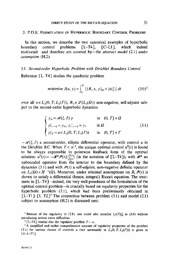
Reference [L-T41 studies the quadratic problem

minimizeJ(u, y)=j’{(R, y, Y)~+ Iu~$} dt (3.0)3 0

over all u E L,(O, T; L*(r)), RI E 9(&(Q)) non-negative, self-adjoint sub- ject to the second-order hyperbolic dynamics

i

Ytt = 45,a Y in (0, T] x 52

Ylr=O= Yo, Yrlr=o= Yl in 52 (3.1)

Ylr=uEJ%O, T;&(O) in (0, T] XT

-&(<, 8) a second-order, elliptic differential operator, with control u in the Dirichlet B.C. When T< co4, the unique optimal control u’(t) is found to be always expressible ion pointwise feedback form of the optimal solution: u’(t) = -99*9’(t)l$,~$ (in the notation of [L-T4]), with Z#* an unbounded operator from ;he interior to the boundary defined by the dynamics (3.1) and with P(t) a self-adjoin& non-negative definite operator on L*(Q) x H-‘(Q). Moreover, under minimal assumptions on R, s(t) is shown to satisfy a differential (hence, integral) Riccati equation. The treat- ment in [L-T4]-indeed, the very well-posedness of the formulation of the optimal control problem-is crucially based on regularity properties for the hyperbolic problem (3.1), which had been preliminarily obtained in [L-Tl]-[L-T2]’ The connection between problem (3.1) and model (2.1) subject to assumption (H.2) is discussed next.

3 Because of the regularity in (2.8) one could also penalize ]~(T)]~ in (3.0) without introducing serious extra diffkulties.

’ [L-T41 studies also the regulator problem T= co. ‘A simplified and rather comprehensive account of regularity properties of the problem

(3.1) for various classes of controls u (not necessarily in L,(O, T, L*(r))) is given in [L-L-T-I].

505/64/l-3

32 DA PRATO, LASIECKA, AND TRIGGIANI

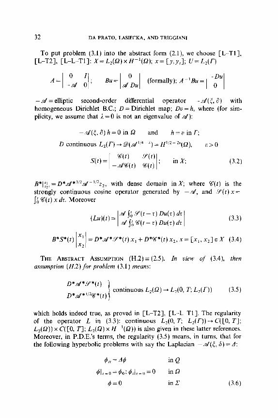
To put problem (3.1) into the abstract form (2.1), we choose [L-T1 1, [L-T2], [L-L-Tl]: X=&(52)x H-‘(G); x= [y,y,]; U=&(T)

-d = elliptic second-order differential operator - zJ( <, 8) with homogeneous Dirichlet B.C.; D = Dirichlet map; Du = h, where (for sim- plicity, we assume that A = 0 is not an eigenvalue of ~4):

-&‘({,a)h=O in Sz and h=v inr,

D continuous L,(T) + 9(&‘/4-8) = W-zc(a), EL-0

S(t) = Wt) Y”(t) . -dW(t) V(t) ’ in X; (3.2)

B*l;;l =D*J$‘*~/~~-“~~~, with dense domain in X; where W(t) is the strongly continuous cosine operator generated by -&, and Y(t) x = j& G??(t) x dz. Moreover

(Lu)(t) = d 1; Y(t - z) Du(z) dz

d j(, V( t - z) Du(r) dT (3.3)

B*S*(t) x1 I I

= D*d*Y*(t) x1 + D*%*(t) x2, x = [x,, x2] E X (3.4) x2

THE ABSTRACT ASSUMPTION (H.2)- (2.5). In view of (3.4), then assumption (H.2) for problem (3.1) means:

D*d*Y*(t)

D*&*‘i2W*(t) I continuous L,(B) + L,(O, T; L,(T)) (35)

which holds indeed true, as proved in [L-TZ], [L-L-Tl]. The regularity of the operator L in (3.3): continuous L,(O, T; L,(T)) -+ C([O, T];

L,(Q)) x C(CO, rl; L2WJ) x H-‘(Q)) is also given in these latter references. Moreover, in P.D.E.‘s terms, the regularity (3.5) means, in turns, that for the following hyperbolic problems with say the Laplacian --Pe(l, 6) = A:

(3.6)

DIRECT STUDY OF THE RICCATI EQUATION 33

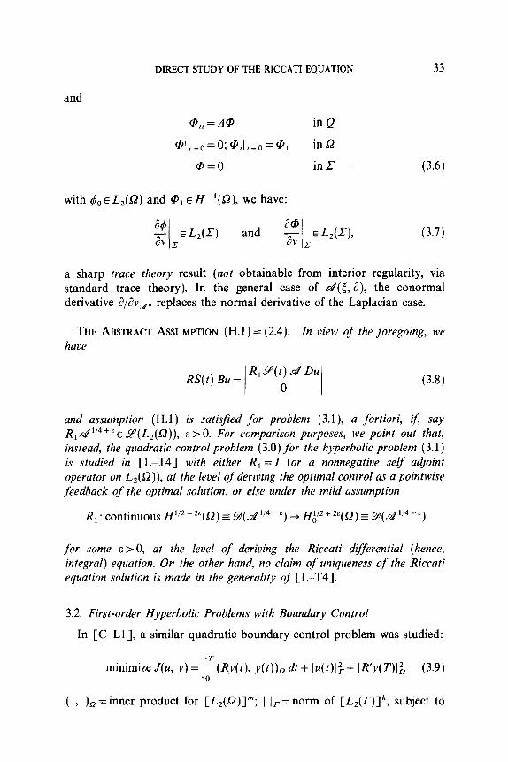
and

Grr = A@ in Q

ql=o=o; @rlr=O’@l in Sz

@=O in C

with &, E L*(G) and @, E H-‘(Q), we have:

and

(3.6)

(3.7)

a sharp truce theory result (not obtainable from interior regularity, via standard trace theory). In the general case of d(<, a), the conormal derivative a/av,. replaces the normal derivative of the Laplacian case.

THE ABSTRACT ASSUMPTION (H.l) = (2.4). In oiew of the foregoing, we have

RS(t) Bu = R,Y(t) ~4 Du

0 (3.8)

and assumption (H.l) is satisfied for problem (3.1), a fortiori, if, say R161’4fE~ S?(L,(Q)), E > 0. For comparison purposes, we point out that, instead, the quadratic control problem (3.0) for the hyperbolic problem (3.1) is studied in [L-T43 with either RI = Z (or a nonnegative self adjoint operator on L,(Q)), at the level of deriving the optimal control as a pointwise feedback of the optimal solution, or else under the mild assumption

R, : continuous H1’2-228(Q) = 9(&1/4-E) + H~Iz+*‘(Q) = 9(~&“‘~+~)

for some E > 0, at the level of deriving the Riccati differential (hence, integral) equation. On the other hand, no claim of uniqueness of the Riccati equation solution is made in the generality of [L-T4].

3.2. First-order Hyperbolic Problems with Boundary Control

In [C-Ll], a similar quadratic boundary control problem was studied:

minimizeJ(u, y)=jT(Ry(t), y(t))S1dt+ lu(t)lF+ IR’y(T)I& (3.9) 0

( , )R= inner product for [L,(Q)]“; I Il-==norm of [L*(Z)]“, subject to

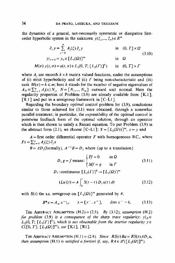
34 DA PRATO, LASIECKA, AND TRIGGIANI

the dynamics of a general, not-necessarily symmetric or dissipative first- order hyperbolic system in the unknown ~$5, ,..., 5,) E R”

‘tY= i Aj(5)ajY in (0, T] x Q j=O (3.10)

Ylt=o= YOE CUQ)Y in Q

Wa) v(t, 0) = 46 0) E L,(O, T; Lmlk) in (0, T] x r

where Aj are smooth k x k matrix valued functions, under the assumptions of (i) strict hyperbolicity and of (ii) r being non-characteristic and (iii) rank M(a) = k < m; here k stands for the number of negative eigenvalues of A,z~~“=~ A,(x) Nj, N= [N, ,..., N,] outward unit normal. Here the regularity properties of Problem (3.9) are already available from [K.l 1, CR.1 ] and put in a semigroup framework in [C-L1 1.

Regarding the boundary optimal control problem for (3.9), conclusions similar to those achieved for (3.1) were obtained, through a somewhat parallel treatment; in particular, the expressibility of the optimal control in pointwise feedback form of the optimal solution, through an operator which is then shown to satisfy a Riccati equation. To put Problem (3.9) in the abstract form (2.1), we choose [C-Ll]: X= [L,(Q))]“, x = y and

A = first order differential operator F with homogeneous B.C., where FX=~~=o A,(t) 8j-X

B = AD,(formally), A - ‘B = D1 where (up to a translation)

I

Ff=O in Q D, g=fmeans:

Mf=g in r (3.11)

D, : continuous [L2(r)lk + [L,(Q)]”

(3.12)

with S(t) the S.C. semigroup on [L2(Q)lm generated by A;

B*x=A,x-1, x= [x-,x+], dimx- =k, (3.13)

THE ABSTRACT ASSUMPTION (H.2) = (2.5). By (3.12), assumption (H.2) for problem (3.9) is a consequence of the sharp trace regularity: ylz E L,(O, T, [L2(r)]‘), which is not obtainable from the interior regularity ye C(CO, Tl; CL2(Q)lmh see WI, WI.

THE ABSTRACT ASSUMPTION (H. 1) = (2.4). Since RS( t ) Bu = RS( t) A D 1 u, then assumption (H.l) is satisfied a fortiori if, say, RA E 2’( [Lz(sZ)]“).

DIRECT STUDY OF THE RICCATI EQUATION 35

By contrast, the control problem study for problems (3.9), (3.10) carried out in [C-L11 requires only a minimal smoothness assumption on R, i.e.: M”E aCuQ)l”) f or any E >O. On the other hand, in such generality, no claim of uniqueness of solution to the Riccati equation is made in [C-Ll].

To conclude this section, we point out that reference [V-J11 minimized the functional (3.9) for Problem (3.10) with R =0 and R’: [Hi]“-+ CJuQ)l”~ a very special case of [C-L1 1. Moreover, the variational techni- ques, used in [V-J11 do not allow extension to penalization of the trajec- tory as in (3.9), R # 0. These last two restrictions are removed in [C-Ll].

Finally, reference [R2] studies symmetric hyperbolic problems in one space dimension through the method of characteristics (which is well known to fail in several space variables).

Lookin, variable

as in [Fl

4. PROOF OF MAIN THEOREM

4.1. Preliminary Changes of Variables

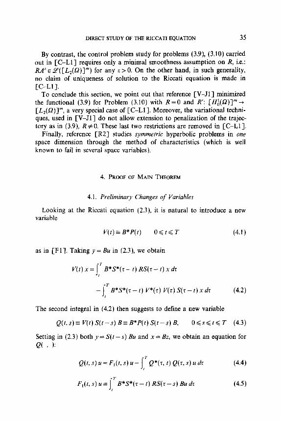
g at the Riccati equation (2.3), it is natural to introduce a new

V(t) E B*P(t) O<t6T

1. Taking y = Bu in (2.3), we obtain

(4.1)

V(t) x= i‘r B*S*(z - t) RS(z - t) x dT f

- ‘B*S*(-C-t) V*(z) V(z)S(r-t)xdz s (4.2) *

The second integral in (4.2) then suggests to define a new variable

Q(t,s)=V(t)S(t-ss)B=B*P(t)S(t-s)B, O<s<t<T (4.3)

Setting in (2.3) both y = S(t - S) Bu and x = Bz, we obtain an equation for Q( 7 1:

Q(f, s) u = F,(t, 8) ~4 - j,’ Q*(T, t) Q(T, 3) u dT

s

T

F,(t, s) 24 = B*S*(z - t) RS(z -3) Bu dz I

(4.4)

(4.5)

36 DA PRATO, LASIECKA, AND TRIGGIANI

Moreover, because of (4.3) we rewrite (4.2) as

V(t)x=F,(t)x-j’Q*(r-I) V(z)S(r-t)xdz (4.6) f

F*(t) x s [‘B*S*(r - t) RS(z - t) x dz f

(4.7)

Equation (4.4) involves only Q, while Eq. (4.6) couples V and Q. Our task is now to show global unique solutions in Q and I/ for Eqs. (4.4) and (4.6) in appropriate spaces. To this end, we follow an established pattern of argument [DaPl], [EDaPl], etc. It consists of two steps: (i) first, proof of local existence; (ii) next, establishment of global a priori bounds.

4.2. Unique Local Solution to Eq. (4.4)

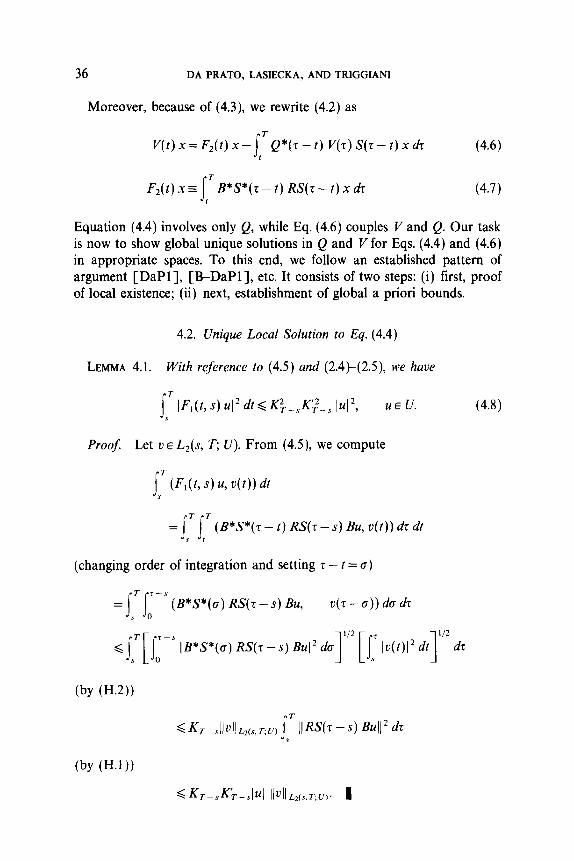
LEMMA 4.1. With reference to (4.5) and (2.4)-(2.5), we have

s T lF,(t, s) u12 dtM.$-,K’,2_s ju12, UE u. (4.8) s

Proof. Let UE L,(s, T; U). From (4.5), we compute

s T (F,(t, s) u, u(t)) dt s = II T T(B*S*(7-t)RS(z-s)Bu,u(t))drdr

s I

(changing order of integration and setting r - t = a)

= (B*S*(a) RS(z -s) Bu, u(z - CT)) da dz

(by W.2))

DIRECT STUDY OF THE RICCATI EQUATION 37

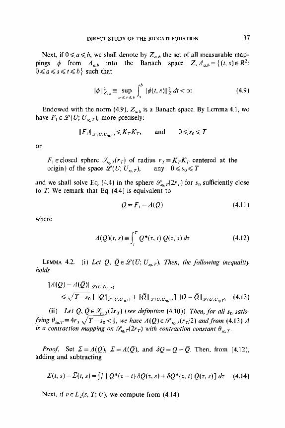
Next, if 0 < ad b, we shall denote by Za,b the set of all measurable map- pings 4 from dU,b into the Banach space Z, A,, = {(t, S) E R*: O<a<s<t<b} such that

(4.9)

Endowed with the norm (4.9), Z,, is a Banach space. By Lemma 4.1, we have F, E .Y( U; US,,T), more precisely:

IlFl II ~p(u;u~o,T~ 6 KJG and O<s,<T

or

F, E closed sphere P&(r=) of radius rT = KTKT centered at the origin) of the space Y( U; U,sO, T), any O<s,<T

and we shall solve Eq. (4.4) in the sphere YS0,(2r,) for s0 sufftciently close to T. We remark that Eq. (4.4) is equivalent to

Q=F,-/I(Q) (4.11)

where

(4.12)

LEMMA 4.2. (i) Let Q, 0 E 9(U; U,,.). Then, the following inequality holds

Gt:IT--s, CllQll,,.;u,,,,+ IIQll,,,;,o,,,l IIQ-Qll,,u;r,~e~,,, (4.13)

(ii) Let Q, Q E 9&(2r,) (see definition (4.10)). Then, for all s,, satis-

fving eso, T = 4r,Jx<f, we have A(Q)E~‘~&~J~) andfrom (4.13) A is a contraction mapping on 9&.(2r,) with contraction constant OSO,T.

Proof: Set z= A(Q), z= A(Q), and SQ = Q-Q. Then, from (4.12), adding and subtracting

Z(t, s) -Z(t, s) = s: [Q*(r - t) 6Q(z, s) + 6Q*(z, t) Q(T, s)] dz (4.14)

Next, if v E L,(s, T; U), we compute from (4.14)

38 DA PRATO, LASIECKA, AND TRIGGIANI

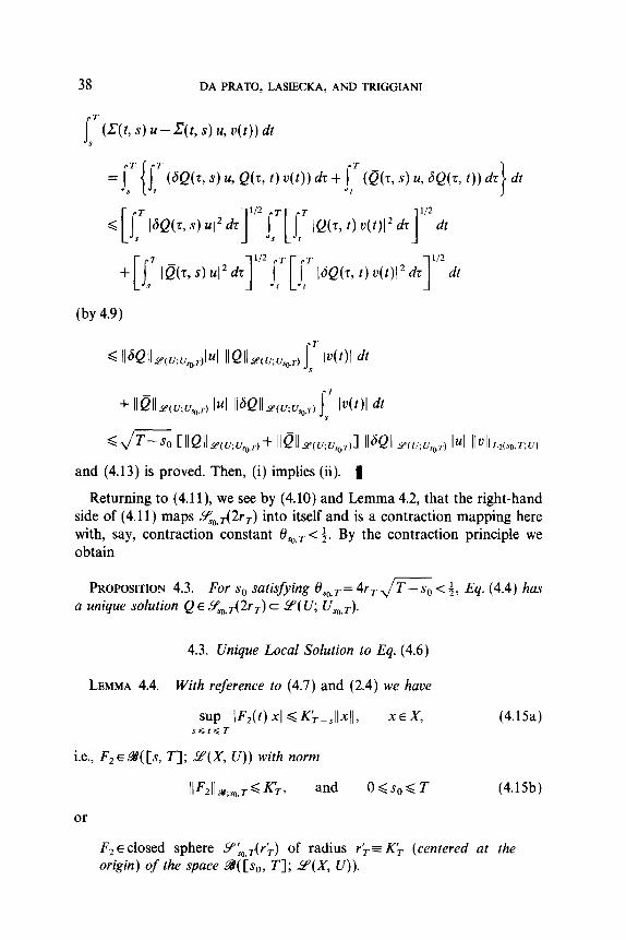
s T(Z(t,s)u-~(t,s)u,u(t))dt s

= (&AT, 8) u, Q(G t) u(t)) dz + IT @(t, s) u, SQ(z, t)) dr dt f

<

(by 4.9)

@+o CllQll,,,;u,,,+ ll~lLc~u~~J Il~Qll,,.;u,,,, I4 Il~Il~,~s,,,w~

and (4.13) is proved. Then, (i) implies (ii). 1

Returning to (4.1 l), we see by (4.10) and Lemma 4.2, that the right-hand side of (4.11) maps 9&.(2r,) into itself and is a contraction mapping here with, say, contraction constant OSO,T < $. By the contraction principle we obtain

hOPOSITION 4.3. For s,, satisfying es&T= 4rT ,/G -C 4, Eq. (4.4) has a UniqUe SdUtiOn Q E y&.(bT) C die( u; u,,T).

4.3. Unique Local Solution to Eq. (4.6)

LEMMA 4.4. With reference to (4.7) and (2.4) we have

SUP IF,(t) XI 4 K’T-,IixII, XEX, (4.15a) S<l<T

i.e., F2 E a( [s, T]; 2(X, U)) with norm

llFzll~;,~,T=T, and O<s,<T (4.15b)

or

F2 E closed sphere YLO,T(r)T) of radius r; c Kk (centered at the origin) of the space W([s,, T]; 2’(X, U)).

DIRECT STUDY OF THE RICCATI EQUATION 39

ProoJ From (4.7), using (H.l)

s

T-I

(f-2(t) x, u) = (S(a) x, RS(a) Bu) da 0

We remark that Eq. (4.6) is equivalent to

V= F2 -y(V) (4.16)

where

(4.17)

and Q( , ) is obtained locally from Proposition 4.3.

PROPOSITION 4.5. Let IlS(t)ll Y4p(xj < const,, 0 < t < T. With so satisfying 6&T = const .4,/c so rT < 4 and with Q( , ) the local solution provided by Proposition 4.3 in q0,T(2rT), then Eq. (4.6) admits a unique solution VEyi,T(2r>) cGf([s,, T]; 2(X, U)) (see definition in (4.15b)).

Prooj Let VEY&.(~+). From (4.7)

I(r( J’)(t) x, u)l = jT (V(T) St? - t) x, Q(T, t) ~1 dz ,

dconstTl~V1l,;,,T~~llxll [jTIQW)ul’d~]l’z f

d constT2r; Jr-so 2rTllxll IuI

and y( V)E~&(I$/~), so that y iS a contraction mapping on Y&T(2r;). Then, by (4.15b), the right-hand side of (4.16) is a contraction mapping on Y:,,T(2r>) with contraction constant 13&, and the contraction principle applies. 1

Remark 4.1. Once Q and hence V are found, we then have a solution P(t) of the Riccati equation (2.3), now rewritten by (4.1) and (4.3) as

P(t)=j-TS*(r-t)RS(r-t)dr-j-TS*(r-t) V*(z) V(z)S(z-t)dz. (4.18) * I

P(t) possesses (by now locally, but after Sect. 4.3, globally) the properties

40 DA PRATO, LASIECKA, AND TRIGGIANI

mentioned in the Main Theorem. The proof of the Main Theorem is com- plete, once we show-in Section 4.4 below-global a priori bounds.

4.4. A Priori Estimates

To obtain a priori bounds for Q and I’, we shall follow an approach which is inspired by the quadratic optimal control problem. It consists-as in the parabolic (analytic semigroup) case for Dirichlet B.C. [Fl], [Da P-Ill-in introducing an evolution operator (which describes the optimal feedback dynamics, in fact). The resulting procedure may be viewed as an appropriate re-arrangement of the ingredients present in the study of the optimal control problem-our guide here being the treatment given in [L-T4]+xcept that our starting point is now the Riccati equation (2.3), not the optimality conditions of the control problem as in [ L-T4].

LEMMA 4.6. With V/E L&?( [s,,, T]; 9(X, U)) with norm I( VII,;,,,.prouided locally by Proportion 4.5, the integral equation:

@(z - t) x = S(z - t) x-j= S(z - a) W(a) @(a, t) x da, XEX (4.19)6 I

admits, for t sufficiently close to T, sO < t, a unique solution

@( ., t): continuous X+ C( [t, T]; X) (4.20)

which possesses the evolution properties:

@(o, cr) = z; w, 0) @(% 3) = @(? s), t<s<a<z

Prooj As in Sections 4.24.3, for h E L2(t, T; X) and @ E 9(X; X,.) we compute, using (H.2)

S(z - a) H’(a) @(o, t) x da, h(z) >

dr

< (I~(I,;,,J' j'[ j7 II@(a, t) xllzd~]"2 [so" lB*S*WW12 d+'dt I I

By contraction principle as before, we then get @( ., t) xeL2(t, T; X). Rewriting (4.19) as

@(z, t)x=S(z-t)x- {L,[V(.)@(~, t)x]}(z) (4.21)

6 Eq. (4.19) defines the optimal dynamics of the optimal control problem.

DIRECTSTUDYOFTHERICCATIEQUATION 41

(see (2.10)), and invoking the continuity (2.10b) of L, with I’( .) @( ., t) x E L2(t, T; U), we then obtain @(., t) XE C( [t, 7’1; X), hence (4.20). 1

LEMMA 4.7. The local solution P(t) of (2.3) provided by Remark 4.1 and the local evolution @J( *, t) provided by Lemma 4.6 are related by

P(t)x=j?Y*(T-t) R@(z, t)x, XEX (4.22) I

ProoJ: See Appendix. [

Remark 4.2. Because of (4.1), the evolution @ obtained by (4.19) may depend on P( . ). Thus, at this stage, (4.22) is not yet a defining formula for P(t). An expression for @ exclusively in terms of the original dynamics (2.1) and the operator R is given next in (4.23), at which point, then, (4.22) becomes a defining formula for P(t). 1

LEMMA 4.8. With L,, LT given by (2.8)-(2.9), we have

@(qt)x={[Z,+L,L,?R]-‘S(.-t)x}(z) (4.23)

where the inverse operator exists and is bounded on all of L2(t, T; X). Explicitly, (4.23) becomes:

@(z, t) = S(T - t) -jr ST S(t - a) B B*S*(r - a) R@(r, t) dr da. (4.24) f 0

Proof. By (2.7) and (4.22), we can rewrite V(t) in (4.1) as

V(t) 5 B*P(t) x= {L*R@(., t) x}(t), XEX (4.25)

Thus, with L* = L: (after t, see (2.11))

V(o) @(a, t)x= L*R@(., o) @(o, t)x= {L:R@(*, t)x}(o) (4.26)

Inserting (4.26) into (4.21) yields (4.23) with the inverse operator well defined and bounded on L,(t, T; X) [L-T43. 1

An improvement of Lemma 4.8 is

LEMMA 4.9. The operator [Z, + L, L*R] = [Z, + L,L: R] occuring in (4.23) is indeed invertible on all of C( [t, T]; X), uniformly in t:

II CZ, + LJ*RI -III L?(c([t,r];x) G constn Obt<T. (4.27)

42 DA PRATO, LASIECKA, AND TRIGGIANI

Proof: We preliminarly establish that:

L,L*R is continuous C([t, r]; X) -+itself, t, <t < T, with a bound, say, less than 1 (independent on t,), provided t, is suf- ficiently close to T.

To prove (4.28), let v E C( [t, T]; X) and recall the continuity (2.10b) of L,:

IILL*W.)Il c(ct, T-I; x) G KTIIL*Rv(. )Il~~(t,w) (4.29)

Next, from (2.7) using a change of order of integration and (H.2)

= <T Is u IB*S*(a- T) Rv(a)l* dz do f I

G (T- t) ~II~IIlI~ll~~~r,~,;~~ (4.30)

and (4.28) follows by (4.29)-(4.30). Now, (4.28) implies that [I, + L,L*R]-’ is continuous C( [t, T]; X) +

itself, t, < t $ T, with a bound indepedent on t,, for ti sufficiently close to T. Thus, after a finite number of steps, such local inversion yields the global inversion (4.27), as in [Da P-111. m

COROLLARY 4.9. The following uniform bound for the evolution operator holds

II @(r, t)ll ucxj 9 con&-, O<t<zdT. (4.31)

Proof: By Lemma 4.8, (4.23) and Lemma 4.9, (4.27). 1

PROPOSITION 4.10 (global boundfor V). For VEW([S~, T]; 2(X, U)) provided by Proposition 4.5, the following uniform bound holds,

IIUB;O,T= SUP IVtJ-4 <con%-, XE x IIXII G 1, (4.32) OCIGT

i.e., VE~([O, T]; 2(X, U)).

Proof: By (4.22) and (4.1)

I( V(t) x, u)l = j’(B*S*(z - t) R@(z, t) x, u) dT f

= T (@(T, t) x, RS(z - t) Bu) dzl

DIRECT STUDY OF THE RICCATI EQUATION 43

(and using Corollary 4.9, (4.31) and (H.l))

<constrKTllxll Iul. I

PROPOSITION 4.11 (global bound for Q). For Q E 9’( U; US,, T) provided by Proposition 4.3, the following uniform bund holds

oslf~~~~~lQ(t,~)~12dt$const.lu12, UE u, (4.33) . .

i.e., Q E 6p(U; U,,.).

Proof. We return to (4.4) which, in view of (4.3), we rewrite as

Q(t,s)x=F,(t,s)x+*S*(T-t) V*(~)Q(~,s)xdz f

=F,(t,s)x-LL,*V*(.)Q(.,s)x (4.34)

where by the regularity (2.1 lb) and Proposition 4.10, (4.32), with s,, <s, we have

Thus in (4.35), we can make the contraction constant <f, for s sufficiently close to T. In view of (4.10), after a finite number of steps on the linear equation (4.34) we obtain Q E LZ’( U; U,,.). 1

Remark 4.3. An alternative, yet closely related treatment for Section 4.4 may be as follows. It uses explicitly and directly only assumptions (H.O)-(H.2) not the properties of L and L* implied by them.

STEP 1. We begin by considering Eq. (4.24)’ in the unknown @( , ) and we then show simultaneously that

’ This can be motivated by thinking of B, at first, as E E U( U; A’). Then, on the maximal existence interval, the Riccati differential equation is

P'+A*P+P(A-BV)+R=O, P(T)=0 (*I

I f @ ( , ) is the evolution operator of A - BV, then P(u) = j: S*(T - c) R@(T, c) da is the uni- que solution of (*). Inserting then V(u)=B*P(u) into the optimal dynamics (4.19) yields (4.24). For B unbounded, we study (4.24) directly to assert the existence of @( , ).

44 DA PRATO, LASIECKA, AND TRIGGIANI

(i) (4.24) admits a unique local solution in @([t, T]; 9(X)) on to < t < z < T, for to sufficiently close to T, moreover,

(ii) the uniform bound (4.31) attains

ll@(? t)ll L?(X) 1 <const.,O<t<r<T.

Proof of Step 1. As in [Da P-111, take T- h <s 6 t < T, for some suf- ficiently small h > 0. Then,

I r

IW S(t - a) BB*S*(z -a) R@(T, s) x dr do, y

s IJ >I

’ ’ = lj j

(B*S*(z - cr) R@(T, s) x, B*S*(t - cr) y) da dz s s

+ j= j’ (B*S*(T -CT) R@( T, s) x, B*S*(t - a) y) da dT I s

t

j [j

T--s 112

1 [j

t-s

1 112

d IB*S*(a) R@(T, s) xl2 dcr IB*S*(fl) y12 4 dT s 0 I-z

T

+I I,

7-s 112 t-s 112 (B*S*(a) R@(T, s) xl2 dcc

I C--r 1 [J P*s*UV y12 @ 1 dz 0

(by W.2))

ML ll~llllyllC(~-$1 sup II@(z> s)xll + (T- t) sup ll@(~> ~1 XIII S<?Cl r<r<?-

G1yzT-s Il~lIIl~ll(T-$1 SUP Il@(~,s)-4 (4.36) S<T<T

and the bound in (4.36) can be made, say, <j by taking h sufficiently small. The contradiction principle then gives, as before, part (i) with to = T-h, and after a finite number of steps one obtains part (ii), using a uniform a priori estimate of P(.) as in [DaP-11 1.

STEP 2. We next proceed through Lemma 4.1, hence Proposition 4.10, finally Proposition 4.11.

Final Remark. We point out, as anticipated in Remark 3.3, that if instead of (H.l) we assume the stronger hypothesis

T IIR”‘S(t) &II2 dtbconst. ]u12, UEU (4.37)

then our proof greatly simplifies. In fact, after the local existence of sec- tions 4.24.3, we can obtain an a priori bound, for Q( , ) directly and

DIRECT STUDY OF THE RICCATI EQUATION 45

trivially from the Riccati equation (2.3). Indeed, setting x = y = Bu in (2.3) yields via (4.3) and (4.37)

Thus, Q E 8(U; U,,T), as desired. With the a priori bound for Q established, we return to Eq. (4.6) linear in V. Then, the contraction argument in Proposition 4.5 leads to a contraction constant which depends only on the interval s0 d s < T. After a finite number of steps, we extend the local solution V into a global solution VE B( [O, T]; 9(X, 17)).

This simple argument for existence and uniqueness of a non-negative selfadjoint solution p(t) of the Riccati equation (2.3) under Assumption (4.37) may be contrasted with the lengthier and more complicated argument given in [P-S11 for the optimal control problem under the same Assumption (4.37). 1

APPENDIX I: PROOF OF LEMMA 4.7 (for BE S?( U; X, see footnote 7)

We wish to show formula (4.22) as a consequence of the Riccati equation (2.3) and of the dynamics (4.19) for @.

STEP 1. We first verify that’ for x, y E X:

i‘ b*WS+r)x, B*P(T)S(~-~),V)~Z ,

= i‘l (S*(r - t) R 1’ S(z - a) BB*P((r) @(c, t) x da, y) dz (A.1) I I

To this end, we use (4.19)

s T (B*P(T) S(z - t) x, B*P(z) S(r - t) y) dz ,

@(q r) x + j7 S(z - a) BB*P(a) @(o, t) x da ,

B*P(z) S(z - t) y >

dr

s The need for this verification is seen by inserting @(z, t) given by (4.19) into formula (4.22) and comparing the resulting expression with the Riccati equation (2.3).

46 DA PRATO, LASIECKA, AND TRIGGIANI

B*P(r) S(7 - t) y dz 64.2)

where we have set

M(t) = jT (B*P(z) @(7, t) x, B*P(z) S(7 - t) y) dz I (A.3)

We now change the order of integration in (A.2): this is legal due to the &(a, T; U)-regularity of B*P(z) S(r - O) Bx = Q(7, a) x in 7, already established in Proposition 4.3. We obtain for the R.H.S. (right hand side) of (A.2):

R.H.S. of (A.2) = M(t) + jt= joT ( B*P(z) S(7 - a) BB*P(a) @(a, t) x,

B*P(z) S(7 -a) S(cr - t) y) dz da (A.4)

(for the internal integration in (A.4) we use (2.3) with t replaced by a, x replaced by BB*P(o) @(a, t) x, and y replaced by S(a - t) y)

(S*(7 - CJ) RS(7 -a) BB*P(o) @(a, t) x, S(a - t) y) dt

- (P(a) BB*P(am y)} da

By (A.3) After further change of the order of integration we get

R.H.S. of (A.2) = j’ (S*(7 - t) R j’S(7 -0) BB*P(a) @(o, t) x do, y) dz I ,

and (A.l) is vert>ed.

STEP 2. We return to the Riccati equation (2.3), and use we use (A.l)

(P(t)x, y)= jTS*(r-t)RS(r-t)xdr, y) ( I

- ( j 1

TS*(7-t)Rj7S(t-o)BB*P(a)@(o,t)xda,y dz f >

(A.5)

and recalling (4.19) in (AS) yields the desired formula (4.22).

DIRECT STUDY OF THE RICCATI EQUATION 47

REFERENCES

WI

WI

A. V. BALAKRISHNAN, “Applied Functional Analysis” 2nd ed. Springer-Verlag, New York/Berlin, 1976 A. V. BALAKRISHNAN, Boundary control of parabolic equations: LQR theory, in “Proc. 5th Internat. Summer School, Central Inst. Math. Acad. Sci., German Democratic Republic Berlin, 1977.

[B-DaPl] V. BARBU AND G. DA F'RATO, “Hamilton-Jacobi Equations in Hilbert Spaces,” Pitman, London, 1983.

[C-Ll] S. CHANG AND I. LASIECKA, Riccati equations for nonsymmetric and non-

[DaPl ]

[DaP-II]

iIF11

WI

[ L-L--T1 ]

[L-T11

[L-T21

[L-T33

[L-T41

[P-Sl]

WI

CR21

[V-J11

dissipative hyperbolic systems with &-boundary control, J. Math. Anal. Appl., in press. G. DA PRATO, Quelques resultats d’existence, unicite et regularite pour un probleme de la theorie du controle, J. Mad Pures Appl. 52 (1973), 353-375. G. DA PRATO AND A. ICHIKAWA, Riccati equations with unbounded coeffkients, Scuola Normale Sup. Pisa, preprint May 1984. F. FLANDOLI, Riccati equations arising in a boundary control problem with dis- tributed parameters, SIAM J. Control Optim. 22 (1984), 7686. H. 0. KREISS, Initial boundary value problems for hyperbolic systems, Comnr. Pure Appl. Math. 13 (1970), 277-298. I. LASIECKA, J. L. LIONS, AND R. TRIGGIANI, Non-homogeneous boundary value problems for second-order hyperbolic operators, J. Math. Pures Appl., in press. I. LASIECKA AND R. TRIGGIANI, A cosine operator approach to modelling L,(O, r; L*(T))-boundary imput hyperbolic equations, Appl. Math Optim. 7 (1981) 35-93. I. LA~IECKA AND R. TRIGGIANI, Regularity of hyperbolic equations under L,(O, T; L,(D))-Dirichlet boundary terms, Appl. Math. Optim. 10 (1983), 275-286. I. LASIECKA AND R. TRIGGIANI, Dirichlet boundary control problem for parabolic equations with quadratic cost: analyticity and Riccati’s feedback syn- thesis, SIAM J. Control Optim. 21 (1983), 41-67. I. LASIECKA AND R. T~IGGIANI, Riccati equations for hyperbolic partial differen- tial equations with L,(O, p, L,(T))-Dirichlet boundary controls, SIAM J. Con- trol Optim., in press. A. PRITCHARD AND D. SALOMON, “The Linear Quadratic Optimal Control Problem for Infinite Dimensional Systems with Unbounded Input and Output Operators,” Mathematics Research Center, Univ. of Wisconsin, Technical Report 2624, 1984. J. RAUCH, L2 is a countinuable initial condition for Kreiss’ mixed problems, Comm. Pure Appl. Math. 25 (1972), 265-285. D. L. RUSSELL, Quadratic performance criteria in boundary control of linear symmetric hyperbolic systems, SIAM J. Conrol Optim. 11 (1973), 475-509. R. VINTER AND T. JOHNSON, Optimal control of non-symmetric hyperbolic systems in n-variables on the half-space, SIAM J. Control Optim. 15 (1977), 129-143.