A Decision Support Tool Coupling a Causal Model and a Multi-objective Genetic Algorithm

M. Ali and F. Esposito (Eds.): IEA/AIE 2005, LNAI 3533, pp. 628 – 637, 2005. © Springer-Verlag Berlin Heidelberg 2005

A Decision Support Tool Coupling a Causal Model and a Multi-objective Genetic Algorithm

Ivan Blecic1, Arnaldo Cecchini1, and Giuseppe A. Trunfio2

1 Department of Architecture and Planning, University of Sassari, Italy ivan, [email protected]

2 Center of High-Performance Computing, University of Calabria, Rende (CS), Italy [email protected]

Abstract. The knowledge-driven causal models, implementing some inferential techniques, can prove useful in the assessment of effects of actions in contexts with complex probabilistic chains. Such exploratory tools can thus help in “fore-visioning” of future scenarios, but frequently the inverse analysis is required, that is to say, given a desirable future scenario, to discover the “best” set of actions. This paper explores a case of such “future-retrovisioning”, coupling a causal model with a multi-objective genetic algorithm. We show how a genetic algo-rithm is able to solve the strategy-selection problem, assisting the decision-maker in choosing an adequate strategy within the possibilities offered by the decision space. The paper outlines the general framework underlying an effective knowl-edge-based decision support system engineered as a software tool.

1 Introduction

When undertaking actions and strategies, a decision-maker normally has to cope with the complexity of the present and future context these strategies will fall in. For the purpose of our research, we can assume that “acting” is always explicitly or implicitly oriented with the intent to make a desirable future scenario more probable (and make the undesirable one less probable). However, the frequently complex interactions among possible social, natural or technological factors can make extremely difficult to take decisions, especially if there are strong constraints. This difficulty can be re-lated to the fact the actors tend to consider only the first-order, or at most the second-order potential effects, being unable to cope intuitively with long cause-effect chains and influences, such that could sometimes bring about quite counter-intuitive and unexpected consequences. For the purpose of adequately taking into account and of coping reliably with the actual system's complexity, it might show useful to build a causal model and its related computational technique.

A widely used approximate technique is the so called Cross-Impact Analysis (CIA) [1], which provides estimated probabilities of future events as the result of the ex-pected (i.e. estimated) interactions among them. Such approach was originally pro-posed by Helmer and Gordon in the 1966. Subsequently, Gordon and Hayward have developed a stochastic algorithmic procedure, capable of proving quantitative results [2]; the idea had number of variants and applications [3-6]. Such causal models and the related computational-inferential techniques made possible the simulation of

A Decision Support Tool Coupling a Causal Model and MOGA 629

effects of subsets of implemented actions on the probability of the final scenarios. However, that brought about the issue of the inverse problem: given a desirable sce-nario, how to find the optimal set of actions in terms of effectiveness and efficiency, which could make the desirable scenario most probable?

In this paper we will propose and exploit a multi-objective genetic algorithm (MOGA) approach in the search for the best set of actions and the related budget allocation problem in the outlined probabilistic context. The computational frame-work described here, coupling the causal model and the MOGA, has been imple-mented is a software tool and is being used as an effective knowledge-based decision support system (DSS).

2 The Dynamics of a System of Events

Let us consider a time interval t∆ and the set

1 , , Ne e=Σ … (1)

whose elements we will call non recurrent events, events which can occur at most once in the time interval [ 0t , 0t t+ ∆ ]. Furthermore assume that, during the given time interval, the occurrence of an event can modify the probability of other events (i.e. the set Σ represents a system). Noticeably, the interactions among events can be signifi-cantly complex, given the possibility of both feedbacks and memory-effect (i.e. the events' probability can depends on the order of occurrences of events).

We can define the state of Σ as an N-dimensional vector s=(s1,...,sN), where si=1 if the i-th event has occurred, otherwise si=0 (i.e. every occurrence of an event triggers a state transition). Between the initial time 0t and the final time 0t t+ ∆ , the system Σ performs, in general, a number of state transitions before reaching the final state.

Every non occurred event ie in a state sk has, with respect to the next state transi-tion, a probability of occurrence ip which can vary during the system's evolution.

Fig. 1. The state-transition diagram for a three-event system without memory

Fig. 2. A scheme of the Cross Impact Analysisapproach

As an example, let us consider the three-event no-memory system 1 2 3 , , e e e=Σ .

The state-transition diagram is represented in the Fig. 1, where all states are labelled using letters from A to H. When the system is in the state C, it has the transition prob-ability pCE (i.e. the current p1) to switch to the state E.

Eventually, at the end the system reaches a state called scenario where, in general, we may observe that some events have occurred during the given time interval. In

a

630 I. Blecic, A. Cecchini, and G.A. Trunfio

particular, observing the entire evolution of the system over time, we can define the probability of occurrence of the event ie , which will be indicated as ( )iP e , or the

probability of non-occurrence, indicated as ( )iP e¬ . Also, it is possible to determine

the joint probabilities, such as ( )i j kP e e e∧ ¬ ∧ ∧" .

Clearly, only the knowledge of all transition probabilities allows us to determine such probabilities referred to the whole time interval. Unfortunately, given N events, the number of possible state transitions is 12NN − (e.g. 5.120 for 10 events) in a non memory-dependent system, and about !eN (e.g. about 10 millions for 10 events) in a memory-dependent system [4]. As numbers grow, the problem becomes increasingly intractable. Nevertheless, as explained in detail further below, an alternative is given by applying Monte Carlo-like stochastic simulations on the cross-impact model [2].

2.1 An Approximate Solution: The Cross-Impact Analysis Approach

As widely known [7], a stochastic simulation procedure permits the estimation of probabilities from a random series of scenarios generated by a causal model. Hence, a possible approach to the former problem is to develop a causal model such as the CIA [1,2], which allows the execution of a stochastic inferential procedure (see Fig. 2). In the majority of cross-impact schemes [2,3,4], every event first gets attributed an initial probability and then it is assumed that, during the system's evolution along the time interval, an event occurrence can modify other events' probability. Thus, the model is specified with the assignment of 2N probabilities:

- for each event ek with k=1...N, an initial a priori probability ˆ ( )keΠ is assigned,

estimated under the hypothesis of the non-occurrence of all the other events; - for each ordered couple of events (ei, ej), with i j≠ , an updated probability

( )j ieΠ is assigned, defining the causal influence of ej over ei, and representing

the new probability of ei under the assumption of the occurrence of ej.

It is important to point out that the updated probabilities introduced above are not the conditional probabilities as defined in the formal probability theory. Instead, they should be intended as new a priori probabilities based upon a newly assumed knowl-edge on the state of the system [4]. Also, it is worth noting that there are formalised procedures allowing a panel of experts to produce knowledge-based estimates of the above probabilities (e.g. see [8]).

Frequently [2,4], the updated probabilities ( )j ieΠ are not assigned explicitly, but

using a relation ( ) ( ( ), )j i i ije e fφΠ = Π , where ( )ieΠ is the probability of ei before the

occurrence of ej, while fij is an impact factor specifying the “intensity” of the effects of the ej over the probability of occurrence of ei.

As shown elsewhere [2], defining the elements of the model (i.e. the initial prob-

abilities ˆ ( )keΠ and the probability updating relations) is the basis for executing M

stochastic simulations of the system's evolution. The procedure is briefly illustrated in the Algorithm 1. In a Monte Carlo fashion, at the end of the execution procedure, the matrix Q contains M stochastically generated scenarios, making possible to estimate the probability of an arbitrary scenario as the frequency of occurrence.

631

1. A N M× integer matrix Q and the integer k are initialised by zeros; 2. while ( k<M )

2.1 all events are marked as non-tested; 2.2 while ( there exist non tested events )

2.1.1 a non-tested event ei, which has probability ( )ieΠ , is randomly selected and is marked as tested;

2.1.2 a random number [0,1]c ∈ is generated; 2.1.3 if ( c < ( )ieΠ ) then

- [ , ] [ , ] 1i k i k← +Q Q ; - all probabilities are updated using the equation ( ) ( ( ), )i j j jie e fφΠ = Π ;

2.1.4 endif 2.3 end while 2.4 1k k← + ;

3. end while

Algorithm 1. The stochastic procedure for the scenario probabilities estimation

The cross-impact model employed by us presents some differences with respect to the classical formulations. In particular, for the purpose of a better representation of a decision-making context, we are assuming that the system's entities are differentiated and collected into three sets

, ,Σ =< >E U A (2)

where E is a set of NE events; U is a set of NU unforeseen events, i.e. external events (exogenous to the simulated system) whose probability can not be influenced by the events in E; A is a set of NA actions, which are events whose probabilities can be set to one or zero by the actor, and can thus be considered as actions at his/her disposal. We assume that the occurrence of events (normal and unforeseen) and actions can influence the probabilities of ie ∈ E . In particular the causal model is specified with:

- the NE events ie ∈ E , each characterised by its initial probability ˆ ( )ieΠ , esti-

mated assuming the single event as isolated;

- the NU unforeseen events iu ∈ U , each defined by a constant probability ˆ ( )iuΠ ;

- each action a ∈ A is defined as , a Iµµ=< > , where Iµµ ∈ is an effort repre-

senting the "resources" invested in an action (e.g. money, time, energy, etc.).

The interactions among entities are defined by three impact factor groups and some interaction laws. In particular we have three matrices, FUE, FEE, and FAE, whose ge-neric element [ , ]ij MAX MAXf f f∈ − determines, as explained below, a change of the

probability of the event ei, respectively caused by the occurrence of the unforeseen event uj, by the occurrence of the event ej and by the implementation of the action aj.

The impact factors affect the change of the events’ probabilities as follows:

1 ( )( ) , 0

( ) , 0( )

1

ii

i

ij ijMAX

j iij

ijMAX

ee f f

f

e fe

ff

− ΠΠ × ≥

Π =Π <

⎧ +⎪⎪⎨ ⎛ ⎞⎪ × +⎜ ⎟⎪ ⎝ ⎠⎩

(3)

A Decision Support Tool Coupling a Causal Model and MOGAa


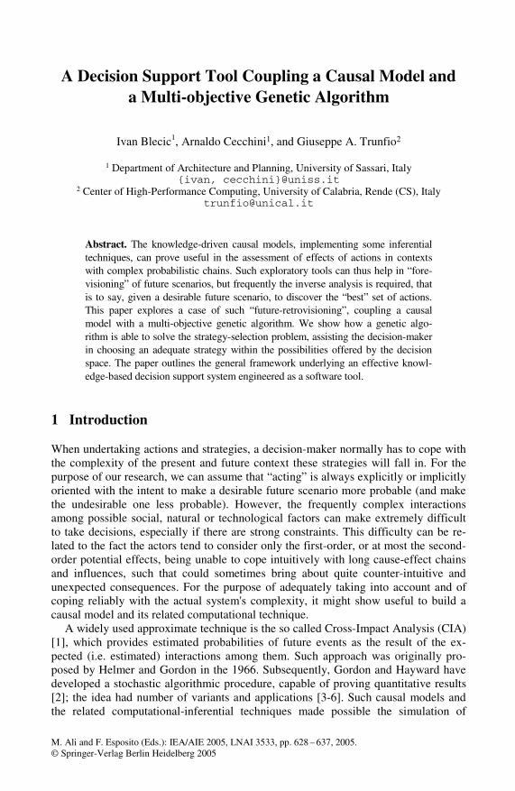
where ( )j ieΠ is the updated probability (see Fig. 3-a). Note that the expression (3)

works in a common-sense fashion: the resistance to change grows as the values gets closer to its limits.

In order to account for the different kinds of effort-impact responses, each action ai is characterised by an impact intensity iψ expressed as a function of the action effort

(see Fig. 3-b). The actual action's impact factors are obtained multiplying the maxi-mum action impact factor in FAE by iψ . The idea is that the more an actor “invests” in

an action, the greater is the action's influence on the system. In particular, for each action, the effective effort interval is defined as [ , ]i i i iα µ µΩ = , with ]0,1[iα ∈ ,

where iµ and i iα µ are the efforts corresponding to respectively the 99% and the 1%

of the maximum action's impact. Clearly, the iα can be close to 1 in case of actions which are not reasonably scalable. Hence the impact intensity ( )ψ µ is defined as:

1( )

1 a be µψ µ − −=+

, where 2 1

( 1)

c ca

α µ−=−

and 1 2 1

c cb

αα−=

− (4)

with 1 ln[(1 0.01) / 0.01]c = − and 2 ln[(1 0.99) / 0.99]c = − .

As in the classical cross-impact models, defining all model's entities, parameters and equations, allows us to perform a series of M stochastic simulations using the procedure illustrated in the Algorithm 1. Subsequently, any scenario probability can be estimated as the frequency of occurrence.

(a)0

0.1

0.2

0.3

0.4

0.5

0.6

0.7

0.8

0.9

1

0 0.1 0.2 0.3 0.4 0.5 0.6 0.7 0.8 0.9 1

f/fmax= –0.8

f/fmax= –0.6

f/fmax= –0.2

f/fmax= –0.9

f/fmax=0.2

f/fmax=0.9

f/fmax=0.8

f/fmax=0.6

f/fmax=0.4 f/fmax= –0.4

∆Π(f/fmax= –0.2)

∆Π(f/fmax=0.2)

µ

0

0.2

0.4

0.6

0.8

1

ψA(µ

)

c µ=

0.99

µ99

c µ=0

.75

c µ=0.

50c µ=0.

25c µ=0.

05

(b)

Fig. 3. (a) how the impact factor f affects probabilities of events; (b) how the action's effort µ affects the impact intensity of actions

3 Searching for the Best Strategies

When the system is highly complex, some aid for the automatic scenario analysis is required. In particular, the most frequent need is the determination of a strategy (i.e.

633

efforts to allocate on every potential action) which is optimal with respect to some objective functions. The problem can be stated as follows.

First we can assume that a joint probability P (i.e. the probability of a scenario) is expressed as a probabilistic function of the effort vector 1 2( , , , )ANµ µ µ=m … repre-

senting a strategy, being iµ the effort “invested” in ai. Then, let us consider a parti-

tion of the set E in three subsets: G, the set of the positive events; B, the set of the negative events; I = E \ G U B, the set of neutral events.

Assuming that events belonging to the same subset are equally important, we want to find the strategy m able to simultaneously maximise the joint probability of events belonging to G and minimise the joint probability of events belonging to B. The search may include the strategy effort minimisation, and some effort constraints. Hence:

1

max ( ), ( ) ( )

max ( ), ( ) ( )

min ( ), ( )AN

i

P e e

P e e

mµ µ

δ δ

δ δ

δ δ

∈Ω

∈Ω

∈Ω

⎧ = ∀ ∈⎪⎪ = ¬ ∀ ∈⎨⎪

=⎪⎩

∑

G Gm

B Bm

m

m m G

m m B

m m

(5)

with the constraint max( ) µδ µ≤m , where Ω is the parameter space and maxµ is the

maximum allowed effort. The objective functions in (5) are not available in explicit form, and their values

can be computed only executing a complete simulation, as illustrated under 2.1. That makes the use of a classic optimisation methods, such as those gradient-based, rather difficult. All that suggests the employment of a technique based on the local function knowledge such as Genetic Algorithms (GAs). In our case, a GA is used to evolve a randomly initialised population, whose generic element is a chromosome representing the NA-dimensional vector m. The i-th gene of the chromosome is obtained as the binary encoding of iµ , using a suitable bit numbers and its interval of definition iI .

Each chromosome can be decoded in a strategy m and, performing the stochastic simulation, the objective functions in (5) can be computed.

In general, the constrained optimisation problem of q scalar functions ( )iφ x , where

∈ Ωx , being Ω the decision space, can be stated as:

max ( ) with 1i i qφ∈Λ

=x

x … , where: : ( ) 0, 1... ia g a i mΛ = ∈ Ω ≤ = (6)

Often, the conflicts among criteria make difficult to find a single optimum solution. Methods for reducing the problem (6) to a single criteria exist, but they are too sub-jectively based on some arbitrary assumption [9].

In a different and a more suitable approach, the comparison of two solutions with respect to several objectives may be achieved through the introduction of the concepts of Pareto optimality and dominance [9-13]. This avoids any a priori assumption about the relative importance of individual objectives, both in the form of subjective weights or as arbitrary constraints. In particular, considering the optimisation problem (6), we say that a solution x dominates the solution y if:



1, , , ( ) ( ) 1, , : ( ) ( )i i k ki m k mφ φ φ φ∀ ∈ ≥ ∧ ∃ ∈ >x y x y… … (7)

In other words, if x is better or equivalent to y with respect to all objectives and better in at least one objective [10,11]. A non-dominated solution is optimal in the Pareto sense (i.e. no criterion can be improved without worsening at least one other criterion). On the other hand, a search based on such a definition of optimum almost always produces not a single solution, but a set of non-dominated solutions, from which the decision-maker will select one.

In the present work, the employed approach for the individual classification is the widely used Goldberg’s ‘non-dominated sorting’ [10]. Briefly, the procedure proceeds as follows: (i) all non-dominated individuals in the current population are assigned to the highest possible rank; (ii) these individuals are virtually removed from the popula-tion and the next set on non-dominated individuals are assigned to the next highest rank. The process is reiterated until the entire population is ranked.

The MOGA (see Algorithm 2) proceeds on the basis of such ranking: every indi-vidual belonging to the same rank class has the same probability to be selected as a parent. The employed GA makes use of elitism as suggested by the recent research in the field [13], which means that from one generation to another, the non-dominated individuals are preserved. This allows us to extract the Pareto-set from the last popu-lation. In order to maximise the knowledge of the search space, the Pareto-optimal solutions have to be uniformly distributed along the Pareto front, so the GA includes a diversity preservation method (i.e. the procedure Filter in Algorithm 2). Just as in single-objective GAs, the constraints are handled by testing the fulfilment of the crite-ria by candidate solutions during the population creation and replacement procedures.

1. Initialise randomly the population P of size NP accounting for the constraints 2. 0k ← 3. while ( k K< )

3.1 Evaluate the objective functions for each individual in P 3.2 Execute the non-dominated sorting and rank the population P 3.3 Copy in the set C all elements x P∈ which have the highest rank 3.4 ( )C Filter C← 3.5 while ( #C< NP )

3.5.1 Select randomly from P, on the basis of their rank and without replace-ment, the two parents 0 0,x y P∈ ;

3.5.2 Perform the uniform crossover producing two children 1 1,x y ; 3.5.3 Perform the children mutation with probability pm producing 1 1,x y ; 3.5.4 if ( the constraints are fulfilled ) then 1 1 , C C x y← ∪ ; 3.5.5 else 00 , C C x y← ∪ ;

3.6 end while 3.7 P C← ; 3.8 1k k← + ;

4. end while 5. C ← Non-dominated elements of P

Algorithm 2. The used elitist multi-objective GA. The Filter procedure eliminates the elements which are closer than an assigned radius, using the Euclidean distance in the decision space. At the end of the procedure, the set C contains the Pareto-optimal solutions

635

4 An Example Application

The coupled CIA-GA presented here has been adopted in a DSS, developed in C++. The software can visualise the definition of the model as a directed graph (see Fig. 4.), and its main outcome is the best-strategy set, computed on the basis of the user’s classification of events.

Fig. 4. The presented example graph and impact factors in the DSS software

Table 1. The entity characteristics in the presented example

Id Set Description Π e1 G Increase of tourist incomings 0.26 e2 B Population decrease, especially young people 0.35 e3 I Increase of un-skilled immigration 0.12 e4 G High added-value economical activities 0.08 e5 B Increase of traffic congestion 0.42 e6 G Industrial development 0.41 e7 G Increase of real-estate values 0.40 e8 I Population increase their demand for services 0.20 e9 G Agricultural development 0.50

Eve

nts

e10 B Increase of unemployment 0.25

Id Description Π u1 An exceptional flooding 0.06 u2 Increase of demand for agro-biological products 0.64 u3 High competition from emerging countries 0.39 u4 Euro:Dollar - 1:2 0.02

Unf

ores

een

even

ts

u5 Oil crisis 0.21

Id Description λ maxαa1 Better quality of the high-school education 0.30 50 a2 Support for entrepreneurial start-ups 0.10 80 a3 Better services for citizens 0.30 50 a4 Investments in new technologies 0.60 40 a5 Rehabilitation and re-qualification of the historical centre 0.75 50 a6 Measures for environmental protection and territorial preservation 0.50 20 a7 Extension and foundation of new universities 0.80 40 a8 Improvement of collective transportation systems 0.80 30

Act

ions

a9 Support for agricultural development 0.20 20



The example application discussed here is related to a policy-making case-study. The Table 1 reports all entities included in the model and their estimated characteris-tics, as well as the events' rating (i.e. positive, negative and neutral sets). The cross-impact factors are shown in the Fig. 4.

The randomly initialised GA population was composed of 200 chromosomes, each coding a strategy (i.e. the 9 effort values relative to the available actions). For each effort value a 12-bit string was employed.

Fig. 5. The set of computed non-dominated solutions in the space of the objective functions defined in Eq. 5. The selected solution is indicated by the two arrows

a 8 (10%)

a 7 (12%)

a 6 (4%)

a 5 (14%)

a 4 (10%)a 3 (10%)

a 2 (23%)

a 1 (13%)a 9 (4%)

0

10

20

30

40

50

60

70

80

e1 e2 e3 e4 e5 e6 e7 e8 e9 e10

A priori probability

Computed probability

Fig. 6. Effort allocation in the selected solution (the total effort is 272)

Fig. 7. How the event probabilities change in case of the selected solution

The objective function was evaluated performing a 200-iteration Monte Carlo simulation for each individual in the population. Given that the adopted GA was of elitist kind, the values of the objective function relative to the current Pareto set are conveniently stored from one generation into its successors (i.e. the simulations are not re-performed). In every generation, after the ranking, for each selected couple a one-site cross-over and subsequently a children mutation with probability pm=0.003 were applied. In this example, in order to explore the whole decision space, the effort constraints were not considered. The computation was simply terminated after 20 generations (the software allows a real-time monitoring of the Pareto-set evolution). Using a standard PC, less than ten minutes were required for the total computation.

637

The Fig. 5, representing the final non-dominated set, shows how the proposed multi-objective approach allows the user to select a solution from a variety of possi-bilities. Clearly the final selection must be performed on the basis of some additional subjective decision. The selected strategy in our case, corresponding to 272 effort units, is highlighted in Fig. 5. In particular, the Fig. 6 reports the suggested effort allocation and the Fig. 7 reports the variation of the estimated probabilities corre-sponding to the solution.

5 Conclusions

We have presented a decision support tool coupling a classical causal model and a multi-objective genetic algorithm. While coupling a causal model with a single-objective GA is not a novelty (e.g. see [14]), we have shown that the use of a MOGA approach offers the decision-maker the choice of an adequate strategy, extending the knowledge about the variety of possibilities offered by the decision space. In particu-lar, our application shows that the proposed DSS can be particularly useful in assist-ing the decision-making processes related to the future probabilistic scenarios.

References

1. Stover, J., Gordon, T.J. Cross-impact analysis. Handbook of Futures Research, ed. J. Fowles. Greenwood Press, 1978

2. Gordon, T.J., Hayward, H. Initial experiments with the cross-impact method of forecast-ing. Futures 1(2), 1968, 100-116

3. Helmer, O. Cross-impact gaming. Futures 4, 1972, 149–167 4. Turoff, M. An alternative approach to cross-impact analysis. Technological Forecasting

and Social Change 3(3), 1972, 309-339 5. Helmer, O. Problems in Future Research: Delphi and Causal Cross Impact Analysis. Fu-

tures 9, 1977, 17-31 6. Alarcòn, L.F., Ashley, D.B. Project management decision making using cross-impact

analysis. Int. Journal of Project Management 16(3), 1998, 145-152 7. Pearl, J. Evidential Reasoning Using Stochastic Simulation of Causal Models. Artificial In-

telligence, 32, 1987, 245-257 8. Linstone, H.A., Turoff, M. (editors). The Delphi Method: Techniques and Applications,

2002, Available at: http://www.is.njit.edu/pubs/delphibook/index.html 9. Fonseca, C.M., Fleming, P.J. An overview of evolutionary algorithms in multiobjective

optimization. Evolutionary Computation 3 (1), 1995, 1–16 10. Goldberg, D. Genetic Algorithms and Evolution Strategy in Engineering and Computer

Science: Recent Advances and Industrial Applications, 1998, Wiley & Sons 11. Sawaragi Y, Nakayama H, Tanino T. Theory of multiobjective optimization. 1985, Or-

lando, Florida: Academic Press. 12. Srinivas N, Deb K. Multiobjective function optimization using nondominated sorting ge-

netic algorithms. Evolutionary Computation 2(3), 1995, 221-248. 13. C.A. Coello Coello, D.A. Van Veldhuizen, G.B. Lamont, Evolutionary Algorithms for

Solving Multi-Objective Problems, Kluwer Academic Publishers, 2002 14. L. M. de Campos, J. A. Gàmez, and S. Moral. Partial abductive inference in bayesian belief

networks using a genetic algorithm. Pattern Recogn. Lett., 20(11-13):1211–1217, 1999.


A Decision Support Tool Coupling a Causal Model and a Multi-objective Genetic Algorithm

Documents

Transcript of A Decision Support Tool Coupling a Causal Model and a Multi-objective Genetic Algorithm