Neural Networks 78 (2016) 65–74

Contents lists available at ScienceDirect

Neural Networks

journal homepage: www.elsevier.com/locate/neunet

2016 Special Issue

A decentralized training algorithm for Echo State Networks indistributed big data applicationsSimone Scardapane a,∗, Dianhui Wang b, Massimo Panella a

a Department of Information Engineering, Electronics and Telecommunications (DIET), ‘‘Sapienza’’ University of Rome, Via Eudossiana 18, 00184 Rome,Italyb Department of Computer Science and Information Technology, La Trobe University, Melbourne, VIC 3086, Australia

a r t i c l e i n f o

Article history:Available online 18 August 2015

Keywords:Recurrent neural networkEcho State NetworkDistributed learningAlternating Direction Method of MultipliersBig data

a b s t r a c t

The current big data deluge requires innovative solutions for performing efficient inference on large,heterogeneous amounts of information. Apart from the known challenges deriving from high volumeand velocity, real-world big data applications may impose additional technological constraints, includingthe need for a fully decentralized training architecture. While several alternatives exist for training feed-forward neural networks in such a distributed setting, less attention has been devoted to the case ofdecentralized training of recurrent neural networks (RNNs). In this paper, we propose such an algorithmfor a class of RNNs known as Echo State Networks. The algorithm is based on the well-known AlternatingDirectionMethod of Multipliers optimization procedure. It is formulated only in terms of local exchangesbetween neighboring agents,without reliance on a coordinating node. Additionally, it does not require thecommunication of training patterns, which is a crucial component in realistic big data implementations.Experimental results on large scale artificial datasets show that it compares favorably with a fullycentralized implementation, in terms of speed, efficiency and generalization accuracy.

© 2015 Elsevier Ltd. All rights reserved.

1. Introduction

With 2.5 quintillion bytes of data generated every day, we areundoubtedly in an era of ‘big data’ (Wu, Zhu, Wu, & Ding, 2014).Amidst the challenges put forth to the machine learning commu-nity by this big data deluge, much effort has been devoted to ef-ficiently analyze large amounts of data by exploiting parallel andconcurrent infrastructures (Cevher, Becker, & Schmidt, 2014; Chu,Kim, Lin, & Yu, 2007), and to take advantage of its possibly struc-tured nature (Bakir, 2007). In multiple real world applications,however, the main issue is given by the overall decentralized na-ture of the data. In what we refer to as ‘data-distributed learn-ing’ (Scardapane, Wang, Panella, & Uncini, 2015a), training data isnot available on a centralized location, but large amounts of it aredistributed throughout a network of interconnected agents(e.g. computers in a peer-to-peer (P2P) network). Practically, a so-lution relying on a centralized controller may be technologicallyunsuitable, since it can introduce a single point of failure, and it

∗ Corresponding author. Tel.: +39 06 44585495; fax: +39 06 4873300.E-mail addresses: simone.scardapane@uniroma1.it (S. Scardapane),

dh.wang@latrobe.edu.au (D. Wang), massimo.panella@uniroma1.it (M. Panella).

http://dx.doi.org/10.1016/j.neunet.2015.07.0060893-6080/© 2015 Elsevier Ltd. All rights reserved.

is prone to communication bottlenecks. Additionally, training datamay not be allowed to be exchanged throughout the nodes,1 eitherfor its size (as is typical in big data applications), or because par-ticular privacy concerns are present (Verykios et al., 2004). Hence,the agents must agree on a single learnedmodel (such as a specificneural network’s topology and weights) by relying only on theirdata and on local communication between them. In the words ofWu et al. (2014), this can informally be understood as ‘a number ofblind men [...] trying to size up a giant elephant ’, where the giant ele-phant refers to the big data, and the blindmen are the agents in thenetwork. Although this analogy referred in general to data miningwith big data, it is a fittingmetaphor for the data-distributed learn-ing setting considered in this paper, which is graphically depictedin Fig. 1.

With respect to neural-like architectures, several decentral-ized training algorithms have been investigated in the last fewyears. This includes distributed strategies for training standardmultilayer perceptrons with back-propagation (Georgopoulos &Hasler, 2014), support vector machines (Forero, Cano, & Giannakis,

1 In the rest of the paper, we use the terms ‘agent’ and ‘node’ interchangeably, torefer to a single component of a network as the one in Fig. 1.

66 S. Scardapane et al. / Neural Networks 78 (2016) 65–74

Fig. 1. Decentralized inference in a network of agents: training data is distributedthroughout the nodes, all of whichmust converge to a singlemodel. For readability,we assume undirected connections between agents.

2010; Navia-Vázquez, Gutierrez-Gonzalez, Parrado-Hernández, &Navarro-Abellan, 2006), deep networks (Dean et al., 2012) andrandom vector functional-link nets (Scardapane et al., 2015a).These are explored more in depth in Section 2.1. Additionally, de-centralized inference has attracted interest from other researchcommunities, includingWireless Sensor Networks (WSNs) (Predd,Kulkarni, & Poor, 2007), cellular neural networks (Luitel & Ve-nayagamoorthy, 2012), distributed optimization (Boyd, Parikh,Chu, Peleato, & Eckstein, 2011; Cevher et al., 2014), distributed on-line learning (Zinkevich, Weimer, Li, & Smola, 2010), and others.

Much less attention has been paid to the topic of distributedlearning with recurrent neural networks (RNNs). In fact, despitenumerous recent advances (Hermans & Schrauwen, 2013;Martens& Sutskever, 2011; Monner & Reggia, 2012; Sak, Senior, & Beau-fays, 2014; Sutskever, Vinyals, & Le, 2014), RNN training remains adaunting task even in the centralized case, mostly due to the well-known problems of the exploding and vanishing gradients (Pas-canu, Mikolov, & Bengio, 2013). A decentralized training algorithmfor RNNs, however, would be an invaluable tool in multiple largescale real world applications, including time-series prediction onWSNs (Predd et al., 2007), and multimedia classification over P2Pnetworks (Scardapane, Wang, Panella, & Uncini, 2015b).

To summarize, in this paper we are concerned with big datascenarios defined by three characteristics: (i) time-varying (i.e., dy-namic); (ii) distributed in nature, without the possibility ofmovingthe data across the network; and (iii) large in volume. Clearly, theactual definition of this last point will depend on the specific ap-plication, e.g. large volumes in a WSN context have a completelydifferent scale with respect to large volumes in a cluster of com-puters. Nonetheless, in this paper we investigate this problem byconsidering datasets that are 1–2 order ofmagnitudes greater withrespect to previous works on related subjects.

To bridge the gap between distributed learning and RNNs,we propose here a data-distributed training algorithm for a classof RNNs known as Echo State Networks (ESNs) (Jaeger, 2002;Lukoševičius & Jaeger, 2009; Verstraeten, Schrauwen, d’Haene,& Stroobandt, 2007). The main idea of ESNs is to separate therecurrent part of the network (the so-called ‘reservoir’), from thenon-recurrent part (the ‘readout’). The reservoir is typically fixed inadvance, by randomly assigning its connections, and the learningproblem is reduced to a standard linear regression over theweights of the readout. Due to this, ESNs do not required complexback-propagation algorithms over the recurrent portion of thenetwork (Campolucci, Uncini, Piazza, & Rao, 1999; Pearlmutter,1995), thus avoiding the problems of the exploding and vanishinggradients. ESNs have been applied successfully to a wide rangeof domains, including chaotic time-series prediction (Jaeger &Haas, 2004; Li, Han, & Wang, 2012), grammatical inference (Tong,Bickett, Christiansen, & Cottrell, 2007), stock price prediction (Lin,Yang, & Song, 2009), speech recognition (Skowronski & Harris,2007) and acoustic modeling (Triefenbach, Jalalvand, Demuynck,

& Martens, 2013), between others. While several researchershave investigated the possibility of spatially distributing thereservoir (Obst, 2014; Shutin & Kubin, 2008; Vandoorne, Dambre,Verstraeten, Schrauwen, & Bienstman, 2011), as depicted inSection 2.2, to the best of our knowledge, no algorithm has beenproposed to train an ESN in the data-distributed case.

The algorithm that we propose is a straightforward applica-tion of the well-known Alternating Direction Method of Multipli-ers (ADMM) optimization technique, which is used to optimize aglobal loss function defined from all the local datasets. Communi-cation between different agents is restricted to the computationof global averages starting from local vectors. This operation canbe implemented efficiently in the decentralized setting with theuse of the ‘decentralized average consensus’ (DAC) procedure (Bar-barossa, Sardellitti, & Di Lorenzo, 2013; Olfati-Saber, Fax, & Mur-ray, 2007). The resulting algorithm is formulated considering onlylocal exchanges between neighboring nodes, thus making it appli-cable in networkswhere no centralized authority is present. More-over, there is no need of exchanging training patterns which, as westated previously, is a critical aspect in big data applications.

Our proposed algorithm is evaluated over several knownbenchmarks for ESNs applications, related to short-term and mid-term chaotic series prediction and non-linear system identifica-tion, where ESNs are known to achieve state-of-the-art results. Aswe stated before, to simulate a large scale application, we considertraining datasetswhich are roughly 1–2 orders ofmagnitude largerthan previous works. Experimental results show that the ADMM-based ESN trained in a decentralized fashion performs favorablywith respect to a fully centralized approach, regarding speed, ac-curacy, and generalization capabilities.

The rest of the paper is organized as follows. In Section 2 weanalyze related works on decentralized learning for feed-forwardneural networks and support vector machines. Additionally, wedetail previous research on spatially distributing the reservoir.In Section 3 we present the theoretical frameworks necessaryto formulate our algorithm, i.e. the standard ESN frameworkwith a least-square solution in Section 3.1, the DAC procedure inSection 3.2, and the ADMM optimization algorithm in Section 3.3.Them, we formalize the distributed training problem for ESNs inSection 4, and provide an ADMM-based algorithm for its solution.This is the main contribution of the present paper. Sections 5 and6 detail multiple experiments on large scale artificial datasets.Finally, we conclude the paper in Section 7, by pointing out thecurrent limitations of our approach, and possible future lines ofresearch.

Notation

In the rest of the paper, vectors are denoted by boldfacelowercase letters, e.g. a, while matrices are denoted by boldfaceuppercase letters, e.g. A. All vectors are assumed to be columnvectors unless otherwise specified. The operator ∥·∥2 is thestandard L2 norm on an Euclidean space. Finally, the notation a[n]is used to denote dependence with respect to a time-instant, bothfor time-varying signals (in which case n refers to a time-instant)and for elements in an iterative procedure (in which case n is theiteration’s index).

2. Related work

2.1. Data-distributed learning for feed-forward models

As stated in the previous section, several works over the lastfew years have explored the idea of fully decentralized trainingfor feed-forward neural networks and support vector machines(SVMs). We present here a brief overview of a selection of these

S. Scardapane et al. / Neural Networks 78 (2016) 65–74 67

works, which are related to the algorithm discussed in thispaper.

In the context of SVMs, one of the earliest steps in thisdirection was the Distributed Semiparametric Support VectorMachine (DSSVM) presented in Navia-Vázquez et al. (2006). Inthe DSSVM, every local node selects a number of centroids fromthe training data. These centroids are then shared with the othernodes, and their corresponding weights are updated locally basedon an iterated reweighted least squares (IRWLS) procedure. TheDSSVM may be suboptimal, and it requires incremental passingof the support vectors (SVs), or centroids, between the nodes,which in turn requires the computation of a Hamiltonian cyclebetween them. An alternative Distributed Parallel SVM (DPSVM)is presented in Lu, Roychowdhury, and Vandenberghe (2008).Differently from the DSSVM, the DPSVM is guaranteed to reach theglobal optimal solution of the centralized SVM in a finite number ofsteps.Moreover, it considers general strongly connected networks,with only exchanges of SVs between neighboring nodes. Still, theneed of exchanging the set of SVs, reduces the capability of thealgorithm to scale to very large networks. A third approach ispresented in Forero et al. (2010), where the problem is recast asmultiple convex subproblems at every node, and solved with theuse of the ADMM procedure (introduced in Section 3.3). ADMM iswidely employed for deriving decentralized training algorithms inthe case of convex optimization problems, such as the SVM and thealgorithm presented in this paper. Other important applicationsinclude decentralized sparse linear regression (i.e. LASSO) (Mateos,Bazerque, & Giannakis, 2010) and its variations, such as groupLASSO (Boyd et al., 2011).

A simpler approach, not deriving from the distributed opti-mization literature, is instead the ‘consensus-based learning’ (CBL)introduced in Georgopoulos and Hasler (2014). CBL allows totransform any iterative learning procedure (defined in the central-ized case) into a general distributed algorithm. This is achieved byinterleaving the local update steps at every node with global aver-aging steps over the network, with the DAC protocol (detailed inSection 3.2). In Georgopoulos and Hasler (2014) it is shown that,if the local update rule is contractive, the distributed algorithmconverges to a unique classifier. The CBL idea is applied to thedistributed training of a multilayer perceptron, with results com-parable to that of a centralized classifier. In Scardapane et al.(2015a), the authors compare a DAC-based and an ADMM-basedtraining algorithms for a class of neural networks known as Ran-dom Vector Functional-Links (RVFLs). The DAC-based algorithm,albeit heuristic, was found to be competitive with respect to theADMM-based one in terms of generalization accuracy, with an ex-tremely reduced training time. The connections between (Scarda-pane et al., 2015a) and the present paper are further explored inSection 4. An extension of the DAC-based algorithm for RVFLs, in-spired from the CBL framework, is instead presented in Scardapaneet al. (2015b), with an application to several music classificationbenchmarks.

A few additional works from the field of signal processingare also worth citing. Distributed learning using linear modelsand time-varying signals has been investigated extensively in thecontext of diffusion filtering (Cattivelli, Lopes, & Sayed, 2008; DiLorenzo & Sayed, 2013). Clearly, linear models are not capableof efficiently capturing complex non-linear dynamics, which arecommon in WSNs and multimedia applications. Due to this, somealgorithms have been proposed for distributed filtering usingkernel-based methods, which are briefly reviewed in Predd et al.(2007); Predd, Kulkarni, and Poor (2009). However, these sufferfrom the same problems relative to SVMs, i.e., their models growlinearly with respect to the size of all the local datasets. Seealso Honeine, Richard, Bermudez, and Snoussi (2008) for furtheranalyses on this point.

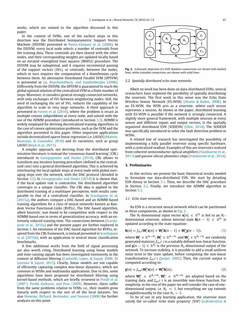
Fig. 2. Schematic depiction of a ESN. Random connections are shown with dashedlines, while trainable connections are shown with solid lines.

2.2. Spatially distributed echo state networks

Albeit no work has been done on data-distributed ESNs, severalresearchers have explored the possibility of spatially distributingthe reservoir. The first work in this sense was the Echo StateWireless Sensor Network (ES-WSN) (Shutin & Kubin, 2008). Inan ES-WSN, the WSN acts as a reservoir, where each sensorrepresents a neuron. As shown in the paper, distributed learningwith ES-WSN is possible if the network is strongly connected. Aslightly more general framework, with multiple neurons at everysensor and different inputs and output vectors, is the spatiallyorganized distributed ESN (SODESN) (Obst, 2014). The SODESNwas specifically introduced to solve the fault detection problem inWSNs.

A related line of research has investigated the possibility ofimplementing a fully parallel reservoir using specific hardware,with a centralized readout. Examples of this are reservoirs realizedfrom coherent semiconductor optical amplifiers (Vandoorne et al.,2011) and passive silicon photonics chips (Vandoorne et al., 2014).

3. Preliminaries

In this section, we present the basic theoretical results neededto formulate our data-distributed ESN. We start by detailingESN theory in Section 3.1. Then, we describe the DAC procedurein Section 3.2. Finally, we introduce the ADMM algorithm inSection 3.3.

3.1. Echo state networks

An ESN is a recurrent neural network which can be partitionedin three components, as shown in Fig. 2.

The Ni-dimensional input vector x[n] ∈ RNi is fed to an Nr -dimensional reservoir, whose internal state h[n − 1] ∈ RNr isupdated according to the state equation:

h[n] = fres(Wri x[n] + Wr

rh[n − 1] + Wroy[n − 1]), (1)

where Wri ∈ RNr×Ni , Wr

r ∈ RNr×Nr and Wro ∈ RNr×No are randomly

generatedmatrices, fres(·) is a suitably defined non-linear function,and y[n − 1] ∈ RNo is the previous No-dimensional output of thenetwork. To increase stability, it is possible to add a small uniformnoise term to the state update, before computing the non-lineartransformation fres(·) (Jaeger, 2002). Then, the current output iscomputed according to:

y[n] = fout(Woi x[n] + Wo

rh[n]), (2)

where Woi ∈ RNo×Ni ,Wo

r ∈ RNo×Nr are adapted based on thetraining data, and fout(·) is an invertible non-linear function. Forsimplicity, in the rest of the paper wewill consider the case of one-dimensional output, i.e. No = 1, but everything we say extendsstraightforwardly to the case No > 1.

To be of use in any learning application, the reservoir mustsatisfy the so-called ‘echo state property’ (ESP) (Lukoševičius &

68 S. Scardapane et al. / Neural Networks 78 (2016) 65–74

Jaeger, 2009). Informally, thismeans that the effect of a given inputon the state of the reservoirmust vanish in a finite number of time-instants. A widely used rule-of-thumb that works well in mostsituations is to rescale the matrix Wr

r to have ρ(Wrr) < 1, where

ρ(·) denotes the spectral radius operator.2 For simplicity, we adoptthis heuristic strategy in this paper, but we refer the readers toYildiz, Jaeger, and Kiebel (2012); Zhang, Miller, and Wang (2012)for recent theoretical results on this aspect.

To train the ESN, suppose we are provided with a sequence ofQ desired input–outputs pairs (x[1], d[1]) . . . , (x[Q ], d[Q ]). Thesequence of inputs is fed to the reservoir, giving a sequence ofinternal states h[1], . . . ,h[Q ] (this is known as ‘state harvesting’or ‘state gathering’). During this phase, since the output of the ESNis not available for feedback, the desired output is used instead inEq. (1) (so-called ‘teacher forcing’). Define the hiddenmatrixH andoutput vector d as:

H =

xT [1] hT[1]

...

xT [1] hT[Q ]

(3)

d =

f −1out (d[1])

...

f −1out (d[Q ])

. (4)

The optimal output weight vector is then given by solving thefollowing regularized least-square problem:

w∗= argmin

w∈RNi+Nr

12

∥Hw − d∥22 +

λ

2∥w∥

22 , (5)

where w =Wo

i Wor

T and λ ∈ R+ is a positive scalar known asregularization factor.3 Solution of problem in Eq. (5) can be obtainedin closed form as:

w∗=HTH + λI

−1 HTd. (6)

More in general, we are provided with a training set S of multipledesired sequences. In this case, we can simply stack the resultinghiddenmatrices and output vectors, and solve Eq. (5). Additionally,we note that in practice we can remove the initial D elements(denoted as ‘dropout’ elements) from each sequence when solvingthe least-square problem, with D specified a-priori, due to theirtransient state. See Jaeger (2002) for a discussion of ESN trainingin the case of online learning.

3.2. Decentralized average consensus

Consider a network of L interconnected agents, as the one inFig. 1, whose connectivity is known a-priori and is fixed. We canfully describe the connectivity between the nodes in the form ofan L × L connectivity matrix C, where Cij = 0 if and only if nodesi and j are connected. In this paper, we assume that the networkis connected (i.e., every node can be reached from another nodewith a finite number of steps), and undirected (i.e., C is symmetric).Additionally, suppose that every node has a measurement vectordenoted by θk[0], k = 1 . . . L.

DAC is an iterative network protocol to compute the globalaverage with respect to the local measurement vectors, requiringonly local communications between them (Barbarossa et al.,

2 The spectral radius of a generic matrix A is ρ(A) = maxi {|λi(A)|}, where λi(A)

is the ith eigenvector of A.3 Since we consider one dimensional outputs, Wo

i and Wor are now row vectors,

of dimensionality Ni and Nr respectively.

2013; Georgopoulos & Hasler, 2014; Olfati-Saber et al., 2007). Itssimplicity makes it suitable for implementation even in the mostbasic networks, such as robot swarms (Georgopoulos & Hasler,2014). At a generic iteration n, the local DAC update is given by:

θk[n] =

Lj=1

Ckjθj[n − 1]. (7)

If the weights of the connectivity matrix C are chosen appropri-ately, this recursive procedure converges to the global averagegiven by Olfati-Saber et al. (2007):

limn→+∞

θk[n] =1L

Lk=1

θk[0], ∀k ∈ {1, 2, . . . , L} . (8)

Practically, the procedure can be stopped after a certain predefinednumber of iterations is reached, or when the norm of the updateis smaller than a certain user-defined threshold δ (see Scardapaneet al., 2015a). In the case of undirected, connected networks, asimple way of ensuring convergence is given by choosing the so-called ‘max-degree’ weights (Olfati-Saber et al., 2007):

Ckj =

1

d + 1if k is connected to j

1 −dk

d + 1if k = j

0 otherwise,

(9)

where dk is the degree of node k, and d is the maximum degreeof the network.4 In practice, many variations on this standardprocedure can be implemented to increase the convergence rate,such as the ‘definite consensus’ (Georgopoulos & Hasler, 2014), orthe strategy introduced in Sardellitti, Giona, andBarbarossa (2010).

3.3. Alternating direction method of multipliers

The final theoretical tool needed in the following section is theADMM optimization procedure (Boyd et al., 2011). ADMM solvesoptimization problems of the form:

minimizes∈Rd,z∈Rl

f (s) + g(z)

subject to As + Bz + c = 0,(10)

where A ∈ Rp×d, B ∈ Rp×l and c ∈ Rp. To solve this, consider theaugmented Lagrangian given by:

Lρ(s, z, t) = f (x) + g(z) + tT (As + Bz + c)

+ρ

2∥As + Bz + c∥2

2 , (11)

where t ∈ Rp is the vector of Lagrangemultipliers, ρ is a scalar, andthe last term is added to ensure differentiability and convergence(Boyd et al., 2011). The optimum of problem in Eq. (10) is obtainedby iterating the following updates:

s[n + 1] = argmins

Lρ(s, z[n], t[n])

(12)

z[n + 1] = argminz

Lρ(s[n + 1], z, t[n])

(13)

t[n + 1] = t[n] + ρ (As[n + 1] + Bz[n + 1] + c) . (14)

Some results on the asymptotic convergence of ADMM can befound in Boyd et al. (2011, Section 3.2). In particular, convergence

4 The degree of a node is the cardinality of the set of its direct neighbors.

S. Scardapane et al. / Neural Networks 78 (2016) 65–74 69

can be tracked by computing the so-called primal and dualresiduals:

r[n] = As[n] + Bz[n] + c, (15)

s[n] = ρATB (z[n] − z[n − 1]) . (16)

ADMM can be stopped after a maximum number of iterations, orwhen both residuals are lower than two pre-specified thresholds:∥r[n]∥2 < ϵprimal∥s[n]∥2 < ϵdual.

Threshold can be chosen based on the combination of a relative andan absolute termination criteria (Boyd et al., 2011):

ϵprimal =√pϵabs + ϵrel max {∥As[n]∥2 , ∥Bz[n]∥2 , ∥c∥2} (17)

ϵdual =√dϵabs + ϵrel

AT t[n]2 (18)

where ϵabs and ϵrel are user-specified tolerances, typically in therange 10−3–10−5.

4. Data-distributed ESN

In this section, we introduce our decentralized training algo-rithm for ESNs. Suppose that the training dataset S is distributedamong a network of nodes, as the one described in Section 3.2.As a prototypical example, multiple sensors in a WSNs can collectdifferent measurements of the same underlying time-series to bepredicted. Additionally, suppose that the nodes have agreed on aparticular choice of the fixed matricesWr

i ,Wrr andWr

o.5 Denote by

Hk and dk the hiddenmatrices and output vectors, computed at thekth node according to Eqs. (3)–(4)with its local dataset. In this case,extending Eq. (5), the global optimization problemcanbe stated as:

w∗= argmin

w∈RNi+Nr

12

L

k=1

∥Hkw − dk∥22

+

λ

2∥w∥

22 . (19)

In theory, distributed least-square problems as the one in Eq. (19)can be solved in a decentralized fashion with two sequential DACsteps, the first of which on the matrices HT

kHk, and the second onthe vectors HT

kdk (Xiao, Boyd, & Lall, 2005). In our case, however,this scheme is impractical to implement due to the typical largesize of the reservoir, making the communication of the matricesHT

kHk a probable network bottleneck.6 More in general, the prob-lem in Eq. (19) can be solved efficiently by distributed optimizationroutines, such as ADMM (Boyd et al., 2011). The idea is to reformu-late the problem by introducing local variables wk for every node,and forcing them to be equal at convergence:

minimizez,w1,...,wL∈RNi+Nr

12

L

k=1∥Hkwk − dk∥

22

+

λ2 ∥z∥2

2 (20)

subject to wk = z, k = 1 . . . L. (21)

The augmented Lagrangian of problem in Eq. (21) is given by:

Lρ(·) =12

L

k=1

∥Hkwk − dk∥22

+

λ

2∥z∥2

2

+

Lk=1

tTk (wk − z) +γ

2

Lk=1

∥wk − z∥22 . (22)

5 There are several strategies to this end. In simple networks, this choice can bepre-implemented on every node. More generally, a single node can be chosen via aleader election protocol, assign the matrices, and broadcast them to the rest of thenetwork.6 A similar issue is explored in Scardapane et al. (2015a, Remark 1).

Algorithm 1: Local training algorithm for ADMM-based ESN at kthnodeInputs: Training set Sk (local), size of reservoir Nr (global),

regularization factors λ, γ (global), maximum number ofiterations T (global)

Output: Optimal output weight vectorw∗

1: Assign matricesWri ,W

rr andWr

o, in agreement with the otheragents in the network.

2: Gather the hidden matrix Hk and teacher signal dk from Sk.3: Initialize tk[0] = 0, z[0] = 0.4: for n from 0 to T do5: Compute wk[n + 1] according to Eq. (23).6: Compute averages w and t by means of the DAC procedure

(see Section 3.2).7: Compute z[n + 1] according to Eq. (24).8: Compute tk[n + 1] according to Eq. (25).9: Compute residuals according to Eqs. (27) and (28), and

check termination criterion.10: end for11: return z[n]

Straightforward computations show that the updates forwk[n+1]and z[n + 1] can be computed in closed form as:

wk[n + 1] =HT

kHk + γ I−1 HT

kdk − tk[n] + γ z[n], (23)

z[n + 1] =γ w + tλ/L + γ

, (24)

where we introduced the averages w =1L

Lk=1 wk[n + 1] and

t =1L

Lk=1 tk[n]. These averages can be computed in a decentral-

ized fashion using a DAC step, as detailed in Section 3.2. Eq. (14)instead simplifies to:

tk[n + 1] = tk[n] + γ (wk[n + 1] − z[n + 1]) . (25)

Eqs. (23) and (25) can be computed locally at every node. Hence,the overall algorithm can be implemented in a purely decentral-ized fashion, where communication is restricted to the use of theDAC protocol. In cases where, on a node, the number of trainingsamples is lower than Nr +Ni, we can exploit the matrix inversionlemma to obtain a more convenient matrix inversion step (Mateoset al., 2010):HT

kHk + γ I−1

= γ −1 I − HTk

γ I + HkHT

k

Hk. (26)

With respect to the training complexity, the matrix inversion andthe termHT

kdk in Eq. (23) can be precomputed at the beginning andstored into memory. Additionally, in this case the residuals in Eqs.(15)–(16) are given by:

rk[n] = wk[n] − z[n], (27)s[n] = −γ (z[n] − z[n − 1]) . (28)

The pseudocode for the algorithm at a local node is provided in Al-gorithm 1.

Remark 1. ESNs admit a particular class of feed-forward neuralnetworks, called Random Vector Functional-Links (RVFLs) (Igelnik& Pao, 1995; Pao & Takefuji, 1992), as a degenerate case. Inparticular, this corresponds to the casewhereWr

r andWro are equal

to the zero matrix. An ADMM-based training algorithm for RVFLswas introduced in Scardapane et al. (2015a). Thus, the algorithmpresented in this paper can be seen as a generalization of that workto the case of a dynamic reservoir.

Remark 2. A large number of techniques have been developed toincrease the generalization capability of ESNs without increasing

70 S. Scardapane et al. / Neural Networks 78 (2016) 65–74

its computational complexity (Lukoševičius & Jaeger, 2009). Pro-vided that the optimization problem in Eq. (5) remains unchanged,and the topology of the ESN is not modified during the learningprocess, many of them can be applied straightforwardly to the dis-tributed training case with the algorithm presented in this paper.Examples of techniques that can be used in this context includelateral inhibition (Xue, Yang, & Haykin, 2007), spiking neurons(Schliebs, Mohemmed, & Kasabov, 2011) and random projections(Butcher, Verstraeten, Schrauwen, Day, & Haycock, 2013). Con-versely, techniques that cannot be straightforwardly applied in-clude intrinsic plasticity (Steil, 2007) and reservoir’s pruning (Scar-dapane, Nocco, Comminiello, Scarpiniti, & Uncini, 2014).

5. Experimental setup

In this section we describe our experimental setup. MATLABcode to repeat the experiments is available on the web under BSDlicense.7 Simulations were performed on MATLAB R2013a, on a64 bit operative system, using an Intel R⃝ CoreTM i5-3330 CPU with3 GHz and 16 GB of RAM.

5.1. Description of the datasets

We validate the proposed ADMM-based ESN on four standardartificial benchmarks applications, related to non-linear systemidentification and chaotic time-series prediction. These are taskswhere ESNs are known to perform at least as good as the stateof the art (Lukoševičius & Jaeger, 2009). Additionally, they arecommon in distributed scenarios. For comparisons between stan-dard ESNs and other techniques, which go outside the scope ofthe present paper, we refer the reader to Lukoševičius and Jaeger(2009) and references therein. To simulate a large scale analysis,we consider datasets that are approximately 1–2 orders of magni-tude larger than previous works. In particular, for every dataset wegenerate 50 sequences of 2000 elements each, starting from differ-ent initial conditions, summingup to 100.000 samples for every ex-periment. This is roughly the limit at which a centralized solutionis amenable for comparison. Below we provide a brief descriptionof the four datasets.

TheNARMA-10 dataset (denoted byN10) is a non-linear systemidentification task, where the input x[n] to the system is whitenoise in the interval [0, 0.5], while the output d[n] is computedfrom the recurrence equation (Jaeger, 2002):

d[n] = 0.1 + 0.3d[n − 1] + 0.05d[n − 1]

×

10i=1

d[n − i] + 1.5x[n]x[n − 9]. (29)

The output is then squashed to the interval [−1, +1] by the non-linear transformation:

d[n] = tanh(d[n] − d), (30)

where d is the empirical mean computed from the overall outputvector.

The second dataset is the extended polynomial (denoted byEXTPOLY) introduced in Butcher et al. (2013). The input is given bywhite noise in the interval [−1 + 1], while the output is computedas:

d[n] =

pi=0

p−ij=0

aijxi[n]xj[n − l], (31)

7 https://bitbucket.org/ispamm/distributed-esn [last visited on 2015-07-06].

where p, l ∈ R are user-defined parameters controlling thememory andnon-linearity of the polynomial,while the coefficientsaij are randomly assigned from the same distribution as the inputdata. In our experiments, we use a mild level of memory and non-linearity by setting p = l = 7. The output is normalized usingEq. (30).

The third dataset is the prediction of the well-known Mackey–Glass chaotic time-series (denoted as MKG). This is defined incontinuous time by the differential equation:

x[n] = βx[n] +αx[n − τ ]

1 + xγ [n − τ ]. (32)

We use the common assignment α = 0.2, β = −0.1, γ = 10,giving rise to a chaotic behavior for τ > 16.8. In particular, in ourexperiments we set τ = 30. Time-series in Eq. (32) is integratedwith a 4th order Runge–Kutta method using a time step of 0.1, andthen sampled every 10 time-instants. The task is a 10-step aheadprediction task, i.e.:

d[n] = x[n + 10]. (33)

The fourth dataset is another chaotic time-series predictiontask, this time on the Lorenz attractor. This is a 3-dimensionaltime-series, defined in continuous time by the following set ofdifferential equations:x1[n] = σ (x2[n] − x1[n])x2[n] = x1[n] (η − x3[n]) − x2[n]x3[n] = x1[n]x2[n] − ζ x3[n],

(34)

where the standard choice for chaotic behavior is σ = 10, η =

28 and ζ = 8/3. The model in Eq. (34) is integrated using anODE45 solver, and sampled every second. For this task, the inputto the system is given by the vector

x1[n] x2[n] x3[n]

, while the

required output is a 1-step ahead prediction of the x1 component,i.e.:

d[n] = x1[n + 1]. (35)

For all four datasets, we supplement the original input with anadditional constant unitary input, as is standard practice in ESNs’implementations (Lukoševičius & Jaeger, 2009).

5.2. Description of the algorithms

In our simulations we generate a network of agents, as theone of Fig. 1, using a random topology model for the connectivitymatrix, where each pair of nodes can be connected with 25%probability. The only global requirement is that the overallnetwork is connected. We experiment with a number of nodesgoing from 5 to 25, by steps of 5. To estimate the testing error, weperform a 3-fold cross-validation on the 50 original sequences. Forevery fold, the training sequences are evenly distributed across thenodes, and the following three algorithms are compared:

Centralized ESN (C-ESN): This simulates the case where trainingdata is collected on a centralized location, and the net istrained by directly solving problem in Eq. (19).

Local ESN (L-ESN): In this case, each node trains a local ESN start-ing from its data, but no communication is performed.The testing error is then averaged throughout the Lnodes.

ADMM-based ESN (ADMM-ESN): This is an ESN trained with thedistributed protocol introduced in Section 4. We set ρ =

0.01, a maximum number of 400 iterations, and ϵabs =

ϵrel = 10−4.

S. Scardapane et al. / Neural Networks 78 (2016) 65–74 71

(a) Dataset N10. (b) Dataset EXTPOLY.

(c) Dataset MKG. (d) Dataset LORENZ.

Fig. 3. Evolution of the testing error (defined as the NRMSE), for networks going from 5 agents to 25 agents. Performance of L-ESN is averaged across the nodes. (Forinterpretation of the references to color in this figure legend, the reader is referred to the web version of this article.)

All algorithms share the same ESN architecture, which is de-tailed in the following section. The 3-fold cross-validation proce-dure is repeated 15 times by varying the ESN initialization and thedata partitioning, and the errors for every iteration and every foldare collected. To compute the error, we run the trained ESN on thetest sequences, and gather the predicted outputs y1, . . . , yK , whereK is the number of testing samples after removing the dropout ele-ments from the test sequences. Then, we compute the NormalizedRoot Mean-Squared Error (NRMSE), defined as:

NRMSE =

Ki=1

yi − di

2|K |σd

, (36)

where σd is an empirical estimate of the variance of the true outputsamples d1, . . . , dK . We note that, in the experiments, the networkis artificially simulated on a single machine. A complete analysis ofthe time required to train ADMM-ESN would require knowledgeof the overhead introduced by the realistic network channel, how-ever, this goes outside the scope of the current paper.

5.3. ESN architecture

As stated previously, all algorithms share the same ESNarchitecture. In this section we provide a brief overview on theselection of its parameters. Firstly, we choose a default reservoir’ssize of Nr = 300, which was found to work well in all situations.Secondly, since the datasets are artificial and noiseless, we set asmall regularization factor λ = 10−3. Four other parameters areinstead selected based on a grid search procedure. The validationerror for the grid-search procedure is computed by performing

a 3-fold cross-validation over 9 sequences, which are generatedindependently from the training and testing set. Each validationsequence has length 2000. In particular, we select the followingparameters:

• The matrix Wri , connecting the input to the reservoir, is

initialized as a full matrix, with entries assigned from theuniform distribution [−αi αi]. The optimal parameter αi issearched in the set {0.1, 0.3, . . . , 0.9}.

• Similarly, thematrixWro, connecting the output to the reservoir,

is initialized as a full matrix, with entries assigned from theuniform distribution [−αf αf]. The parameter αf is searched inthe set {0, 0.1, 0.3, . . . , 0.9}. We allow αf = 0 for the casewhere no output feedback is needed.

• The internal reservoir matrixWrr is initialized from the uniform

distribution [−1 + 1]. Then, on average 75% of its connectionsare set to 0, to encourage sparseness. Informally, a sparseinternal matrix creates ‘clusters’ of heterogeneous featuresfrom its input (Jaeger, 2002; Scardapane et al., 2014). Finally, topreserve stability, the matrix is rescaled so as to have a desiredspectral radius ρ, which is searched in the same interval as αi(see the discussion on the spectral radius in Section 3.1).

• We use tanh(·) non-linearities in the reservoir, while a scaledidentity f (s) = αts as the output function. The parameter αt issearched in the same interval as αi.

Additionally, we insert uniform noise in the state update of thereservoir, sampled uniformly in the interval

0, 10−3

, and we

discard D = 100 initial elements from each sequence.

72 S. Scardapane et al. / Neural Networks 78 (2016) 65–74

(a) Dataset N10. (b) Dataset EXTPOLY.

(c) Dataset MKG. (d) Dataset LORENZ.

Fig. 4. Evolution of the training time, for networks going from 5 agents to 25 agents. Time of L-ESN is averaged across the nodes.

Table 1Optimal parameters found by the grid-search procedure. For a description of theparameters, see Section 5.2.

Dataset ρ αi αt αf Nr λ

N10 0.9 0.5 0.1 0.3

300 2−3EXTPOLY 0.7 0.5 0.1 0MKG 0.9 0.3 0.5 0LORENZ 0.1 0.9 0.1 0

Table 2Final misclassification error and training time for C-ESN, provided as a reference,together with one standard deviation.

Dataset NRMSE Time (s)

N10 0.08 ± 0.01 9.26 ± 0.20EXTPOLY 0.39 ± 0.01 8.96 ± 0.19MKG 0.18 ± 0.03 9.02 ± 0.15LORENZ 0.67 ± 0.01 9.47 ± 0.14

6. Experimental results

The final settings resulting from the grid-search procedure arelisted in Table 1. It can be seen that, except for the LORENZ dataset,there is a tendency towards selecting large values of ρ. Outputfeedback is needed only for the N10 dataset, while it is foundunnecessary in the other three datasets. The optimal input scalingαf is ranging in the interval [0.5, 0.9], while the optimal teacherscaling αt is small in the majority of cases.

The average NRMSE and training times (in seconds) for C-ESNare provided in Table 2 as a reference. Clearly, NRMSE and trainingtime for C-ESN do not depend on the size of the agents’ network,and they can be used as an upper baseline for the results of thedistributed algorithms. Since we are considering the same amount

of training data for each dataset, and the same reservoir’s size,the training times in Table 2 are roughly similar, except for theLORENZ dataset, which has 4 inputs compared to the other threedatasets (considering also the unitary input). As we stated earlier,performance of C-ESN are competitive with the state-of-the-artfor all the four datasets. Moreover, we can see that it is extremelyefficient to train, taking approximately 9 s in all cases.

To study the behavior of the decentralized procedures whentraining data is distributed, we plot the average error for the threealgorithms, when varying the number of nodes in the network,in Fig. 3(a)–(d). The average NRMSE of C-ESN is shown as dashedblack line, while the errors of L-ESN and ADMM-ESN are shownwith blue squares and red circles respectively. Clearly, L-ESN isperforming worse than C-ESN, due to its partial view on thetraining data. For small networks of 5 nodes, this gap may not beparticularly pronounced. This goes from a 3% worse performanceon the LORENZ dataset, up to a 37% decrease in performance for theN10 dataset (going from an NRMSE of 0.08 to an NRMSE of 0.11).The gap is instead substantial for large networks of up to 25 nodes.For example, the error of L-ESN is more than twice that of C-ESNfor the N10 dataset, and its performance is 50% worse in the MKGdataset. Albeit these results are expected, they are evidence of theneed for a decentralized training protocol for ESNs, able to take intoaccount all the local datasets.

As is clear from Fig. 3, ADMM-ESN is able to perfectly trackthe performance of the centralized solution in all situations. Asmall gap in performance is present for the two predictions taskswhen considering large networks. In particular, the performanceof ADMM-ESN is roughly 1% worse than C-ESN for networksof 25 nodes in the datasets MKG and LORENZ. In theory, thisgap can be reduced by considering additional iterations for the

S. Scardapane et al. / Neural Networks 78 (2016) 65–74 73

ADMMprocedure, although thiswould be impractical in realworldapplications.

Training time requested by the three algorithms is shownin Fig. 4(a)–(d). The training time for L-ESN and ADMM-ESN isaveraged throughout the agents. Since the computational time oftraining an ESN is mostly related to the matrix inversion in Eq. (6),training time is monotonically decreasing in L-ESN with respect tothe number of nodes in the network (the higher the number ofagents, the lower the amount of data at every local node). Fig. 4shows that the computational overhead requested by the ADMMprocedure is limited. In the best case, the N10 dataset with 10nodes, it required only 0.3 s more than L-ESN, as shown fromFig. 4(a). In theworst setting, the EXTPOLY datasetwith 15 nodes, itrequired 2.2 smore, as shown fromFig. 4(b). In all settings, the timerequested by ADMM-ESN is significantly lower compared to thetraining time of its centralized counterpart, showing it usefulnessin large scale applications. Once again, it should be stressed thatthis analysis does not take into consideration the communicationoverhead between agents, which depends strictly on the actualnetwork technology. With respect to this point, we note that theDAC procedure has been extensively analyzed over a large numberof realistic networks (Barbarossa et al., 2013), showing competitiveperformance in most situations.

7. Conclusions

In this paper we have introduced a decentralized algorithm fortraining an ESN, in the case where data is distributed through-out a network of interconnected nodes. The proposed algorithmdemonstrated good potential to resolve some benchmark prob-lems where datasets are large and stored in a decentralized man-ner. It has multiple real-world applications in big data scenarios,particularly for large scale prediction over WSNs, or for decen-tralized classification of multimedia data. It is a direct applicationof the ADMM procedure, which we employ in our algorithm be-cause of the following two reasons: (i) communication betweennodes is restricted to local exchanges for the computation of anaverage vector, without reliance on a centralized controller; (ii)there is no need for the nodes to communicate training data be-tween them, which is crucial in big data scenarios. Experimentalresults onmultiple benchmarks, related to non-linear system iden-tification and chaotic time-series prediction, demonstrated that itis able to efficiently track a purely centralized solution, while atthe same time imposing a small computational overhead in termsof vector–matrix operations requested to the single node. Commu-nication overhead, instead, is given by the iterative application ofa DAC protocol. This represents a first step towards the develop-ment of data-distributed strategies for general RNNs, which wouldrepresent invaluable tools in real world applications. Future linesof research involve considering different optimization procedureswith respect to ADMM, or more flexible DAC procedures. Addi-tionally, although in this paper we have focused on batch learn-ing, we envision to develop online strategies inspired to the CBLframework.

References

Bakir, G. (2007). Predicting structured data. MIT press.Barbarossa, S., Sardellitti, S., & Di Lorenzo, P. (2013). Distributed detection and

estimation in wireless sensor networks. In R. Chellapa, & S. Theodoridis (Eds.),E-Reference signal processing (pp. 329–408). Elsevier.

Boyd, S., Parikh, N., Chu, E., Peleato, B., & Eckstein, J. (2011). Distributed optimizationand statistical learning via the alternating direction method of multipliers.Foundations and Trends R⃝ in Machine Learning , 3(1), 1–122.

Butcher, J. B., Verstraeten, D., Schrauwen, B., Day, C. R., & Haycock, P. W. (2013).Reservoir computing and extreme learningmachines for non-linear time-seriesdata analysis. Neural Networks, 38, 76–89.

Campolucci, P., Uncini, A., Piazza, F., & Rao, B. D. (1999). On-line learning algorithmsfor locally recurrent neural networks. IEEE Transactions on Neural Networks,10(2), 253–271.

Cattivelli, F. S., Lopes, C. G., & Sayed, A. H. (2008). Diffusion recursive least-squaresfor distributed estimation over adaptive networks. IEEE Transactions on SignalProcessing , 56(5), 1865–1877.

Cevher, V., Becker, S., & Schmidt, M. (2014). Convex optimization for big data:scalable, randomized, and parallel algorithms for big data analytics. IEEE SignalProcessing Magazine, 31(5), 32–43.

Chu, C.-T., Kim, S. K., Lin, Y. A., & Yu, Y. Y. (2007). Map-reduce for machinelearning on multicore. In Advances in neural information processing systems(pp. 281–288).

Dean, J., Corrado, G., Monga, R., Chen, K., Devin,M., Mao,M., et al. (2012). Large scaledistributed deep networks. In Advances in neural information processing systems(pp. 1223–1231).

Di Lorenzo, P., & Sayed, A. H. (2013). Sparse distributed learning based on diffusionadaptation. IEEE Transactions on Signal Processing , 61(6), 1419–1433.

Forero, P. A., Cano, A., & Giannakis, G. B. (2010). Consensus-based distributedsupport vector machines. The Journal of Machine Learning Research, 11,1663–1707.

Georgopoulos, L., & Hasler, M. (2014). Distributedmachine learning in networks byconsensus. Neurocomputing , 124, 2–12.

Hermans, M., & Schrauwen, B. (2013). Training and analysing deep recurrent neuralnetworks. In Advances in neural information processing systems (pp. 190–198).

Honeine, P., Richard, C., Bermudez, J. C. M., & Snoussi, H. (2008). Distributedprediction of time series data with kernels and adaptive filtering techniquesin sensor networks. In Proceedings of the 42nd Asilomar conference on signals,systems and computers (pp. 246–250). IEEE.

Igelnik, B., & Pao, Y.-H. (1995). Stochastic choice of basis functions in adaptivefunction approximation and the functional-link net. IEEE Transactions on NeuralNetworks, 6(6), 1320–1329.

Jaeger, H. (2002). Adaptive nonlinear system identification with echo statenetworks. In Advances in neural information processing systems (pp. 593–600).

Jaeger, H., & Haas, H. (2004). Harnessing nonlinearity: predicting chaotic systemsand saving energy in wireless communication. Science, 304(5667), 78–80.

Li, D., Han, M., & Wang, J. (2012). Chaotic time series prediction based on a novelrobust echo state network. IEEE Transactions on Neural Networks and LearningSystems, 23(5), 787–799.

Lin, X., Yang, Z., & Song, Y. (2009). Short-term stock price prediction based on echostate networks. Expert Systems with Applications, 36(3), 7313–7317.

Lu, Y., Roychowdhury, V., & Vandenberghe, L. (2008). Distributed parallel supportvector machines in strongly connected networks. IEEE Transactions on NeuralNetworks, 19(7), 1167–1178.

Luitel, B., & Venayagamoorthy, G. K. (2012). Decentralized asynchronous learningin cellular neural networks. IEEE Transactions on Neural Networks and LearningSystems, 23(11), 1755–1766.

Lukoševičius, M., & Jaeger, H. (2009). Reservoir computing approaches to recurrentneural network training. Computer Science Review, 3(3), 127–149.

Martens, J., & Sutskever, I. (2011). Learning recurrent neural networkswith hessian-free optimization. In Proceedings of the 28th international conference on machinelearning, ICML (pp. 1033–1040).

Mateos, G., Bazerque, J. A., & Giannakis, G. B. (2010). Distributed sparse linearregression. IEEE Transactions on Signal Processing , 58(10), 5262–5276.

Monner, D., & Reggia, J. A. (2012). A generalized LSTM-like training algorithm forsecond-order recurrent neural networks. Neural Networks, 25, 70–83.

Navia-Vázquez, A., Gutierrez-Gonzalez, D., Parrado-Hernández, E., & Navarro-Abellan, J. J. (2006). Distributed support vector machines. IEEE Transactions onNeural Networks, 17(4), 1091–1097.

Obst, O. (2014). Distributed fault detection in sensor networks using a recurrentneural network. Neural Processing Letters, 40(3), 261–273.

Olfati-Saber, R., Fax, J. A., & Murray, R. M. (2007). Consensus and cooperation innetworked multi-agent systems. Proceedings of the IEEE, 95(1), 215–233.

Pao, Y.-H., & Takefuji, Y. (1992). Functional-link net computing: theory, systemarchitecture, and functionalities. Computer , 25(5), 76–79.

Pascanu, R., Mikolov, T., & Bengio, Y. (2013). On the difficulty of training recurrentneural networks. In Proceedings of the 30th international conference on machinelearning.

Pearlmutter, B. A. (1995). Gradient calculations for dynamic recurrent neuralnetworks: A survey. IEEE Transactions on Neural Networks, 6(5), 1212–1228.

Predd, J. B., Kulkarni, S. R., & Poor, H. V. (2007). Distributed learning in wirelesssensor networks. IEEE Signal Processing Magazine, 56–69.

Predd, J. B., Kulkarni, S. R., & Poor, H. V. (2009). A collaborative training algorithm fordistributed learning. IEEE Transactions on Information Theory, 55(4), 1856–1871.

Sak, H., Senior, A., & Beaufays, F. (2014). Long short-term memory recurrentneural network architectures for large scale acoustic modeling. In Proceedingsof the annual conference of international speech communication association,INTERSPEECH.

Sardellitti, S., Giona, M., & Barbarossa, S. (2010). Fast distributed average consensusalgorithms based on advection–diffusion processes. IEEE Transactions on SignalProcessing , 58(2), 826–842.

Scardapane, S., Nocco, G., Comminiello, D., Scarpiniti, M., & Uncini, A. (2014).An effective criterion for pruning reservoir’s connections in echo statenetworks. In 2014 International joint conference on neural networks (IJCNN)(pp. 1205–1212). INNS/IEEE.

Scardapane, S.,Wang, D., Panella,M., & Uncini, A. (2015a). Distributed learningwithrandom vector functional-link networks. Information Sciences, 301, 271–284.

74 S. Scardapane et al. / Neural Networks 78 (2016) 65–74

Scardapane, S., Wang, D., Panella, M., & Uncini, A. (2015b). Distributed musicclassification using random vector functional-link nets. In 2015 Internationaljoint conference on neural networks (IJCNN). INNS/IEEE.

Schliebs, S., Mohemmed, A., & Kasabov, N. (2011). Are probabilistic spikingneural networks suitable for reservoir computing? In 2011 International jointconference on neural networks (IJCNN) (pp. 3156–3163). INNS/IEEE.

Shutin, D., & Kubin, G. (2008). Echo state wireless sensor networks. In 2008 IEEEworkshop on machine learning for signal processing (pp. 151–156).

Skowronski, M. D., & Harris, J. G. (2007). Automatic speech recognition using apredictive echo state network classifier. Neural Networks, 20(3), 414–423.

Steil, J. J. (2007). Online reservoir adaptation by intrinsic plasticity for backpropa-gation–decorrelation and echo state learning. Neural Networks, 20(3), 353–364.

Sutskever, I., Vinyals, O., & Le, Q. V. V. (2014). Sequence to sequence learningwith neural networks. In Advances in neural information processing systems(pp. 3104–3112).

Tong, M. H., Bickett, A. D., Christiansen, E. M., & Cottrell, G. W. (2007). Learninggrammatical structure with echo state networks. Neural Networks, 20(3),424–432.

Triefenbach, F., Jalalvand, A., Demuynck, K., & Martens, J.-P. (2013). Acousticmodeling with hierarchical reservoirs. IEEE Transactions on Audio, Speech andLanguage Processing , 21(11), 2439–2450.

Vandoorne, K., Dambre, J., Verstraeten, D., Schrauwen, B., & Bienstman, P. (2011).Parallel reservoir computing using optical amplifiers. IEEE Transactions onNeural Networks, 22(9), 1469–1481.

Vandoorne, K., Mechet, P., Van Vaerenbergh, T., Fiers, M., Morthier, G., Verstraeten,D., et al. (2014). Experimental demonstration of reservoir computing on asilicon photonics chip. Nature Communications, 5.

Verstraeten, D., Schrauwen, B., d’Haene, M., & Stroobandt, D. (2007). Anexperimental unification of reservoir computing methods. Neural Networks,20(3), 391–403.

Verykios, V. S., Bertino, E., Fovino, I. N., Provenza, L. P., Saygin, Y., & Theodoridis, Y.(2004). State-of-the-art in privacy preserving datamining.ACMSIGMODRecord,33(1), 50–57.

Wu, X., Zhu, X., Wu, G.-Q., & Ding, W. (2014). Data mining with big data. The IEEETransactions on Knowledge and Data Engineering , 26(1), 97–107.

Xiao, L., Boyd, S., & Lall, S. (2005). A scheme for robust distributed sensor fusionbased on average consensus. In Fourth international symposium on informationprocessing in sensor networks, 2005 (pp. 63–70). IEEE.

Xue, Y., Yang, L., & Haykin, S. (2007). Decoupled echo state networks with lateralinhibition. Neural Networks, 20(3), 365–376.

Yildiz, I. B., Jaeger, H., & Kiebel, S. J. (2012). Re-visiting the echo state property.Neural Networks, 35, 1–9.

Zhang, B., Miller, D. J., & Wang, Y. (2012). Nonlinear systemmodeling with randommatrices: echo state networks revisited. IEEE Transactions on Neural Networksand Learning Systems, 23(1), 175–182.

Zinkevich, M., Weimer, M., Li, L., & Smola, A. J. (2010). Parallelized stochasticgradient descent. In Advances in neural information processing systems(pp. 2595–2603).