
a database schema for the analysis of global dynamics of ...
31
A DATABASE SCHEMA FOR THE ANALYSIS OF GLOBAL DYNAMICS OF MULTIPARAMETER SYSTEMS ZIN ARAI * , WILLIAM KALIES † , HIROSHI KOKUBU ‡ , KONSTANTIN MISCHAIKOW § , HIROE OKA ¶ , AND PAWE L PILARCZYK k Abstract. A generally applicable, automatic method for the efficient computation of a database of global dynamics of a multiparameter dynamical system is introduced. An outer approximation of the dynamics for each subset of the parameter range is computed using rigorous numerical meth- ods and is represented by means of a directed graph. The dynamics is then decomposed into the recurrent and gradient-like parts by fast combinatorial algorithms and is classified via Morse decom- positions. These Morse decompositions are compared at adjacent parameter sets via continuation to detect possible changes in the dynamics. The Conley index is used to study the structure of isolated invariant sets associated with the computed Morse decompositions and to detect the ex- istence of certain types of dynamics. The power of the developed method is illustrated with an application to the two-dimensional, density-dependent, Leslie population model. An interactive vi- sualization of the results of computations discussed in the paper can be accessed at the website http://chomp.rutgers.edu/database/, and the source code of the software used to obtain these results has also been made freely available. Key words. database, dynamical system, Conley index, Morse decomposition, Leslie population models, combinatorial dynamics, multiparameter system AMS subject classifications. Primary: 37B35. Secondary: 37B30, 37M99, 37N25, 92-08. 1. Introduction. The global dynamics of a nonlinear system can exhibit struc- tures at all spatial scales, for example, the fractal structures associated to chaotic dynamics. The same phenomenon can occur with respect to the parameters, that is, global dynamical structures can change on Cantor sets in parameter space. From the point of view of scientific computation, only a finite amount of information can be computed, and therefore, any computational characterization of global dynamics of a multiparameter system can be expected to represent a dramatic reduction of informa- tion. Nevertheless, the computation of global dynamical information is an important problem for applications, which leads to the questions of how to characterize global dynamical structures and how to identify changes in these structures in practice. The * PRESTO, Japan Science and Technology Agency / Hokkaido University, Creative Research Initiative ”Sousei”, Sapporo 001-0021, Japan. Partially supported by Grant-in-Aid for Scientific Research (No. 17740054), Ministry of Education, Science, Technology, Culture and Sports, Japan. † Department of Mathematical Sciences, Florida Atlantic University, 777 Glades Rd, Boca Raton, FL 33431. Partially supported by NSF grant DMS-0511208 and DOE grant DE-FG02-05ER25713. ‡ Department of Mathematics, Kyoto University, Kyoto 606-8502, Japan. Partially supported by Grant-in-Aid for Scientific Research (No. 17340045), Ministry of Education, Science, Technology, Culture and Sports, Japan. § Department of Mathematics and BioMaPS, Hill Center-Busch Campus, Rutgers, The State University of New Jersey, 110 Frelinghusen Rd, Piscataway, NJ 08854-8019, USA. Partially supported by NSF grant DMS-0511115, by DARPA, and by DOE grant DE-FG02-05ER25711. ¶ Department of Applied Mathematics and Informatics, Faculty of Science and Technology, Ryukoku University, Seta, Otsu 520-2194, Japan. Partially supported by Grant-in-Aid for Scientific Research (No. 17540206), Ministry of Education, Science, Technology, Culture and Sports, Japan. k Centre of Mathematics, University of Minho, Campus de Gualtar, 4710-057 Braga, Portugal and Department of Mathematics, Kyoto University, Kyoto 606-8502, Japan. Partially supported by the JSPS Postdoctoral Fellowship No. P06039 and by Grant-in-Aid for Scientific Research (No. 1806039), Ministry of Education, Science, Technology, Culture and Sports, Japan. The final version of this preprint has been published in SIAM Journal on Applied Dynamical Systems, Vol. 8, No. 3, 2009, pp. 757–789, DOI: 10.1137/080734935, and is available at journal’s website. 1
-
Upload
khangminh22 -
Category
Documents
-
view
1 -
download
0
Transcript of a database schema for the analysis of global dynamics of ...
A DATABASE SCHEMA FOR THE ANALYSIS OF GLOBALDYNAMICS OF MULTIPARAMETER SYSTEMS
ZIN ARAI∗, WILLIAM KALIES† , HIROSHI KOKUBU‡ , KONSTANTIN MISCHAIKOW§ ,
HIROE OKA¶, AND PAWE L PILARCZYK‖
Abstract. A generally applicable, automatic method for the efficient computation of a databaseof global dynamics of a multiparameter dynamical system is introduced. An outer approximationof the dynamics for each subset of the parameter range is computed using rigorous numerical meth-ods and is represented by means of a directed graph. The dynamics is then decomposed into therecurrent and gradient-like parts by fast combinatorial algorithms and is classified via Morse decom-positions. These Morse decompositions are compared at adjacent parameter sets via continuationto detect possible changes in the dynamics. The Conley index is used to study the structure ofisolated invariant sets associated with the computed Morse decompositions and to detect the ex-istence of certain types of dynamics. The power of the developed method is illustrated with anapplication to the two-dimensional, density-dependent, Leslie population model. An interactive vi-sualization of the results of computations discussed in the paper can be accessed at the websitehttp://chomp.rutgers.edu/database/, and the source code of the software used to obtain theseresults has also been made freely available.
Key words. database, dynamical system, Conley index, Morse decomposition, Leslie populationmodels, combinatorial dynamics, multiparameter system
AMS subject classifications. Primary: 37B35. Secondary: 37B30, 37M99, 37N25, 92-08.
1. Introduction. The global dynamics of a nonlinear system can exhibit struc-tures at all spatial scales, for example, the fractal structures associated to chaoticdynamics. The same phenomenon can occur with respect to the parameters, that is,global dynamical structures can change on Cantor sets in parameter space. From thepoint of view of scientific computation, only a finite amount of information can becomputed, and therefore, any computational characterization of global dynamics of amultiparameter system can be expected to represent a dramatic reduction of informa-tion. Nevertheless, the computation of global dynamical information is an importantproblem for applications, which leads to the questions of how to characterize globaldynamical structures and how to identify changes in these structures in practice. The
∗PRESTO, Japan Science and Technology Agency / Hokkaido University, Creative ResearchInitiative ”Sousei”, Sapporo 001-0021, Japan. Partially supported by Grant-in-Aid for ScientificResearch (No. 17740054), Ministry of Education, Science, Technology, Culture and Sports, Japan.†Department of Mathematical Sciences, Florida Atlantic University, 777 Glades Rd, Boca Raton,
FL 33431. Partially supported by NSF grant DMS-0511208 and DOE grant DE-FG02-05ER25713.‡Department of Mathematics, Kyoto University, Kyoto 606-8502, Japan. Partially supported by
Grant-in-Aid for Scientific Research (No. 17340045), Ministry of Education, Science, Technology,Culture and Sports, Japan.§Department of Mathematics and BioMaPS, Hill Center-Busch Campus, Rutgers, The State
University of New Jersey, 110 Frelinghusen Rd, Piscataway, NJ 08854-8019, USA. Partially supportedby NSF grant DMS-0511115, by DARPA, and by DOE grant DE-FG02-05ER25711.¶Department of Applied Mathematics and Informatics, Faculty of Science and Technology,
Ryukoku University, Seta, Otsu 520-2194, Japan. Partially supported by Grant-in-Aid for ScientificResearch (No. 17540206), Ministry of Education, Science, Technology, Culture and Sports, Japan.‖Centre of Mathematics, University of Minho, Campus de Gualtar, 4710-057 Braga, Portugal and
Department of Mathematics, Kyoto University, Kyoto 606-8502, Japan. Partially supported by theJSPS Postdoctoral Fellowship No. P06039 and by Grant-in-Aid for Scientific Research (No. 1806039),Ministry of Education, Science, Technology, Culture and Sports, Japan.
The final version of this preprint has been published in SIAM Journal on Applied Dynamical Systems,Vol. 8, No. 3, 2009, pp. 757–789, DOI: 10.1137/080734935, and is available at journal’s website.
1
2 Z. Arai, W. Kalies, H. Kokubu, K. Mischaikow, H. Oka, and P. Pilarczyk
fact that this is a nontrivial task has been made clear by the work of the dynamicalsystems community over the last century.
Identifying and classifying the qualitative properties of models over wide ranges ofparameter values is of fundamental importance in many disciplines, and in particularit is of primary interest to many computational biologists [10]. The fact that mosttopics of interest in systems biology are dynamic in nature suggests the need for acomprehensive, yet efficient method for cataloging the global dynamics of nonlinearsystems. In other words, a method is desired which computationally constructs adatabase of global dynamical behavior of a specific system over a range of parameters.
The starting point for our computational methods is Conley’s topological ap-proach to dynamics [2], which we review in the next section. The prior work in[1, 5, 9, 12, 24] has shown that Conley theory is an appropriate theoretical base fordesigning algorithms in computational dynamics. The purpose of this paper is todemonstrate that these ideas can be used to design an efficient computational frame-work for constructing databases of global dynamics of specific systems over multipleparameters. While the methods we propose are general, we illustrate them using aparticular population model which we describe in Section 1.2.
1.1. Preliminary ideas. We restrict our attention to the setting of a multipa-rameter family of dynamical systems given by a continuous function
f : X × Λ 3 (x, λ) 7→ f(x, λ) = fλ(x) ∈ X (1.1)
where the phase space X is a locally compact metric space and the parameter spaceΛ is a compact, locally contractible, connected metric space. Note that we do notassume that fλ is a homeomorphism.
The fundamental structures in any dynamical system are the invariant sets. Aset Z ⊂ X is invariant at λ ∈ Λ if fλ(Z) = Z. Since we cannot perform computationsat each parameter value independently, we are interested in considering sets whichare invariant with respect to a subset of the parameter space. We use the notationF : X × Λ→ X × Λ for the trivial extension of the system to include the parametersas explicit variables defined by
F (x, λ) =(fλ(x), λ
)=(f(x, λ), λ
). (1.2)
For Λ0 ⊂ Λ we denote the restriction of F to X × Λ0 by FΛ0 : X × Λ0 → X × Λ0.Observe that F = FΛ and that fλ is readily identified with Fλ. Moreover, given aset S ⊂ X ×Λ we denote its restriction to Λ0 by SΛ0
:= S ∩ (X ×Λ0). In particular,we often identify Sλ ⊂ X with Sλ = Sλ × λ. In this language, a set S ⊂ X × Λis invariant over Λ0 if FΛ0
(SΛ0) = SΛ0
, which is an equivalent way to state that theset Sλ is invariant at all λ ∈ Λ0.
We wish to identify and characterize a finite collection of invariant sets whichdetermine the global, qualitative behavior of the dynamics. In addition, we need amethod for comparing two invariant sets Sλ0
and Sλ1at distinct parameters. Deciding
what sets to compute and how to compare them are the fundamental issues we attemptto address.
We emphasize that while the amount of information that can be computed isfinite, this does not mean that we cannot detect or characterize dynamical structuresthat occur on arbitrarily small scales. For example, topological techniques can beused to identify chaotic dynamics via a semiconjugacy onto a subshift of finite type,see [12]. Moreover, even though we cannot compute the dynamics at each parameter
A Database Schema for the Analysis of Global Dynamics of Multiparameter Systems 3
separately, this does not mean that we cannot obtain results which apply to everyparameter value. Indeed, the methods we employ do compute mathematically rigorousglobal structures for invariant sets at all parameter values.
1.2. Model example. To provide perspective on the practicality and utility ofour approach, we consider the two-dimensional version of an overcompensatory Lesliepopulation model g : R2 × R4 → R2 given by[
x1
x2
]7→[
(θ1x1 + θ2x2)e−φ(x1+x2)
px1
],
where the fertility rates decay exponentially with population size. This model andits biological relevance is discussed in considerable detail in work of Ugarcovici andWeiss [25]. As indicated there, in view of g(x, θ, p, φ) = φ−1g(φx, θ, p, 1), the constantφ may be scaled arbitrarily, and thus it suffices to study f : R2 × R3 → R2 given by
(x, λ) =
[ x1
x2
],
θ1
θ2
p
7→ f(x, λ) =
[(θ1x1 + θ2x2)e−0.1(x1+x2)
px1
](1.3)
Furthermore, the detailed numerical studies of [25] indicate that this system exhibitsa wide variety of different dynamical behavior, which suggests that it provides ameaningful test for the usefulness of the techniques introduced in this paper.
1.3. Outline of the paper. In the remainder of the paper we develop ourmethod and apply it to the Leslie model. In Section 2 we introduce the dynamicalstructures which we utilize and review Conley theory. In Section 3 we introduce amethod for building a combinatorial representation of the dynamics and a means ofcomparing the computed structures at different parameters. In Section 4 we addressthe question of efficient computational algorithms based on rectangular grids in Xand Λ. In Section 5 we describe a database computed with our methods for the modelexample introduced in Section 1.2 with p = 0.7 and θ1, θ2 varying in selected ranges,and we show how this database can be queried for various dynamical properties.Finally, in Section 6 we briefly mention a result of similar computations where allthree parameters are varied.
2. Review of Conley theory. Recall that a compact set N ⊂ X × Λ0 is anisolating neighborhood for FΛ0 if
Inv (N,FΛ0) ⊂ intX×Λ0(N)
where Inv (N,FΛ0) denotes the maximal invariant set inN under FΛ0 , and intX×Λ0(N)denotes the interior of N with respect to the subspace topology on X ×Λ0. Isolatingneighborhoods are computable and hence provide a means of identifying invariantsets. In particular, an invariant set SΛ0
⊂ X × Λ0 is an isolated invariant set ifSΛ0
= Inv (N,FΛ0) for some isolating neighborhood N .
As indicated in [2, 15], the space of isolated invariant sets is a sheaf. Moreprecisely, if N is an isolating neighborhood for F = FΛ and S = Inv (N,F ), then forany Λ0 ⊂ Λ, NΛ0
is an isolating neighborhood for FΛ0and SΛ0
= Inv (NΛ0, FΛ0
). Inparticular, for any λ ∈ Λ, Sλ ⊂ X × λ is an isolated invariant set for Fλ : X ×λ → X × λ and Sλ ⊂ X is an isolated invariant set for fλ : X → X.
To simplify the presentation and analysis, throughout this paper we make use ofthe following assumption and establish the following notation.
4 Z. Arai, W. Kalies, H. Kokubu, K. Mischaikow, H. Oka, and P. Pilarczyk
A1: There exists a compact set B ⊂ X × Λ which is an isolatingneighborhood for F . Its maximal invariant set is denoted by S :=Inv (B,F ).
Using the sheaf property of isolated invariant sets, SΛ0denotes the restriction of
S to X ×Λ0, which is an isolated invariant set for FΛ0 if Λ0 is compact. As indicatedabove, we are interested in understanding the structure of Sλ for all λ ∈ Λ, and wemake use of two essential ideas due to Conley [2]: Morse decompositions and theConley Index.
2.1. Morse decompositions. Recall that a Morse decomposition of SΛ0 is afinite collection
M(SΛ0) = MΛ0
(p) ⊂ SΛ0| p ∈ PΛ0
of disjoint isolated invariant sets of FΛ0, called Morse sets, which are indexed by the
set PΛ0on which there exists a strict partial order >Λ0
, called an admissible order,such that for every (x, λ) ∈ SΛ0
\⋃p∈PMΛ0
(p) and any complete orbit γ of FΛ0
through (x, λ) in SΛ0there exist indices p >Λ0
q such that under FΛ0
ω(γ) ⊂MΛ0(q) and α(γ) ⊂MΛ0
(p).
Morse decompositions provide a coarse but global description of the dynamics on SΛ0.
Remark 2.1. With regard to the construction of a database for global dynamics,we make several important observations concerning Morse decompositions, see [2, 13].
1. Morse decompositions of SΛ0 are not unique. They can often be refined orcoarsened, and many systems have no finest Morse decomposition.
2. The empty set can be a Morse set.3. Every structure within SΛ0
that is associated with recurrent dynamics, e.g. afixed point, a periodic orbit, or chaotic dynamics, must lie in some Morse set.Away from the Morse sets the dynamics is gradient-like and the direction oftrajectories is captured by an admissible partial order.
4. Given a Morse decomposition, there is a unique minimal admissible partialorder called the flow-defined order. Any extension of the flow-defined orderwhich maintains a strict partial order produces an admissible order.
5. Consider a Morse decomposition M(SΛ0) = MΛ0
(p) ⊂ SΛ0| p ∈ PΛ0
of SΛ0
with admissible order >Λ0 . If Λ1 ⊂ Λ0, then the collection of sets
MΛ1(p) ⊂ SΛ1
| p ∈ PΛ0 ,
where MΛ1(p) := MΛ0
(p)∩ (X ×Λ1), is a Morse decomposition of SΛ1under
FΛ1 with the same admissible order.
Observe that since PΛ0is a strict partially ordered set, a Morse decomposition can
be represented as an acyclic directed graph MG(Λ0) called the Morse graph over Λ0.The elements of the index set PΛ0 , which naturally correspond to the Morse sets, arethe vertices of the Morse graph over Λ0, and the edges of the Morse graph over Λ0 arethe minimal order relations which through transitivity generate >Λ0
. In other words,for p, q ∈ PΛ0
there is a directed edge p→ q in MG(Λ0) if p >Λ0q and there does not
exist r ∈ PΛ0such that p >Λ0
r >Λ0q.
Computationally, we obtain Morse decompositions indirectly, and often it can beestablished by further computation that a Morse set is empty. In that case, such
A Database Schema for the Analysis of Global Dynamics of Multiparameter Systems 5
a set can be removed from the Morse decomposition as described by the followingproposition whose proof follows directly from the definition of a Morse decomposition.
Proposition 2.2. Consider a Morse decomposition M(SΛ0) =MΛ0(p) ⊂ SΛ0 |
p ∈ PΛ0
of SΛ0
with admissible order >. Assume MΛ0(p0) = ∅. Then
M′(SΛ0) := MΛ0(p) ⊂ SΛ0 | p ∈ PΛ0 \ p0
is a Morse decomposition of SΛ0and an admissible order is given by >′ where for all
p, q ∈ PΛ0 \ p0 we have p >′ q if and only if p > q.From Proposition 2.2, if MG(Λ0) is the Morse graph over Λ0 corresponding to
M(SΛ0), then MG′(Λ0), the Morse graph over Λ0 corresponding to M′(SΛ0
), hasvertices PΛ0
\ p0 and has an edge p → q if either p → q is an edge in MG(Λ0) orp → p0 → q are edges in MG(Λ0). The simplified Morse graph MG′(Λ0) is calleda trivial reduction of MG(Λ0). Whenever possible, we work with a trivial reductionof a Morse graph. The possibility that a Morse set is trivial can be detected via theConley index which is described in the next section.
2.2. The Conley index. As explained in Section 3, computational methodsexist to find Morse decompositions, see [1]. The Conley index, which is an algebraictopological invariant of isolated invariant sets, is used to understand the structure ofthe dynamics within a Morse set.
To explain the index we begin by considering an arbitrary continuous map g : Z →Z on a locally compact metric space and a pair of compact sets N = (N1, N0) suchthat N0 ⊂ N1 ⊂ Z. Consider the pointed quotient space
(N1/N0, [N0]
)obtained by
collapsing N0 to a single point [N0]. Define gN :(N1/N0, [N0]
)→(N1/N0, [N0]
)by
gN (x) =
g(x) if x, g(x) ∈ N1 \N0
[N0] otherwise.
The pair N = (N1, N0) is an index pair if the map gN is continuous and cl (N1 \N0)is an isolating neighborhood [21].
The following two facts about index pairs are most relevant and can be found in[2, 13].
1. For any isolated invariant set K, there exists at least one index pair N =(N1, N0) such that K = Inv (cl (N1 \N0), g).
2. For any isolated invariant set K, there can exist many index pairs whichisolate K.
The first fact implies that for any Morse set MΛ0(p) for the system FΛ0 thereexists an index pair N = (N1, N0) such that the induced map FΛ0,N :
(N1/N0, [N0]
)→(
N1/N0, [N0])
is a continuous function and MΛ0(p) = Inv
(cl (N1 \N0), FΛ0
). Passing
to homology leads to a family of group endomorphisms
FΛ0,N∗ : H∗(N1/N0, [N0]
)→ H∗
(N1/N0, [N0]
). (2.1)
The second fact allows for different choices of index pairs which can lead todifferent group endomorphisms. Thus, to define the Conley index of an isolatedinvariant set, such as a Morse set MΛ0
(p), one must consider equivalence classes ofthese group endomorphisms [13]. In constructing our database, we do not utilize thefull Conley index; instead, we store a weaker invariant, namely the nonzero eigenvaluesof FΛ0,N∗ restricted to the torsion-free part of H∗
(N1/N0, [N0]
). This weaker invariant
is chosen because these eigenvalues are readily computed and compared.Remark 2.3. With regard to the construction and interpretation of the database,
there are several important observations about the index to be made, see [13].
6 Z. Arai, W. Kalies, H. Kokubu, K. Mischaikow, H. Oka, and P. Pilarczyk
1. If the Conley index is trivial, then the map FΛ0,N∗ is nilpotent. This im-plies that the eigenvalues of FΛ0,N∗ restricted to the torsion-free part ofH∗(N1/N0, [N0]
)are all zero.
2. The empty set is an isolated invariant set with trivial Conley index. Thus, ifthere are nonzero eigenvalues of FΛ0,N∗ restricted to the torsion-free part ofH∗(N1/N0, [N0]
), then MΛ0
(p) 6= ∅.3. There exist nontrivial isolated invariant sets with trivial Conley index. For
example, consider the logistic map gλ(x) = λx(1−x), λ ∈ [1, 4], and an indexpair N = (N1, N0) =
([−1, 2], −1, 2
). The index map FN∗ is nilpotent, but
clearly Sλ = Inv (N1 \N0, gλ) 6= ∅.4. The Conley index can be used to reconstruct some of the structure of the
dynamics of the associated isolated invariant set. In particular, under appro-priate conditions the Conley index can be used to conclude the existence offixed points, periodic orbits, and chaotic dynamics.
5. Suppose Λ1 ⊂ Λ0 are both contractible. If MΛ0(p) is a Morse set, or indeedany isolated invariant set, then the nonzero eigenvalues of the torsion-freepart of any index map FΛ0,N∗ are identical to the nonzero eigenvalues of thetorsion-free part of any index map FΛ1,N∗ for the set MΛ1
(p) = MΛ0(p) ∩
(X × Λ1).
2.3. Conley-Morse graphs. We are now in a position to describe the funda-mental element of our database. Let Λ0 ⊂ Λ and let M(SΛ0
) = MΛ0(p) ⊂ SΛ0
| p ∈ PΛ0
be a Morse decomposition of SΛ0with admissible order >Λ0
. The Conley-Morse graphover Λ0 of M(SΛ0) is denoted by CMG(Λ0) and consists of MG(Λ0), the Morse graphover Λ0 with the additional information of the nonzero eigenvalues of the torsion-freepart of the index map of each Morse set assigned to the associated node. We presentthis information by labeling each node in the following format.
pk : n→ ∗
denotes the fact that the k-th Morse set has nonzero eigenvalues ∗ on the n-th levelof homology. If the k-th Morse set has no nonzero eigenvalues then we write
pk : 0 .
An example of how this information can be used to describe the structure of thedynamics is given in Proposition 5.8.
As described in Sections 3 and 4, we compute the Conley-Morse graphs overdistinct fixed subregions of parameter space. This raises the question of how to relatethe resulting Conley-Morse graphs. One answer is provided in the following definition.
Definition 2.4. Assume A1. Let Λ0,Λ1 ⊂ Λ be such that Λ0,1 := Λ0 ∩ Λ1 is anonempty, contractible set. Let
M(SΛi) = MΛi(p) ⊂ SΛi | p ∈ PΛi
for i = 0, 1 be Morse decompositions with admissible orders >i. The associated Morsegraphs MG(Λ0) over Λ0 and MG(Λ1) over Λ1 are equivalent if there exists an orderpreserving bijection ι : (PΛ0
, >0)→ (PΛ1, >1) such that
MΛ0(p) ∩ (X × Λ0,1) = MΛ1
(ι(p)
)∩ (X × Λ0,1).
A Database Schema for the Analysis of Global Dynamics of Multiparameter Systems 7
The continuation property of the Conley index [2] implies that if MG(Λ0) andMG(Λ1) are equivalent via the order preserving bijection ι : (PΛ0
, >0) → (PΛ1, >1),
then the Conley-Morse graphs CMG(Λ0) and CMG(Λ1) are also equivalent, that is,the nonzero eigenvalues associated to corresponding Morse sets are identical.
3. Combinatorial representation of dynamics. Conley-Morse graphs arethe key elements of information stored in our database. In this section we describea general procedure for computing these graphs. We begin by describing a means ofcombinatorializing the dynamics.
Recall [17] that a grid on a metric space Z is a collection Z of nonempty, compactsubsets of Z with the following properties:
(a) Z =⋃G∈Z G,
(b) G = cl(int (G)
)for all G ∈ Z,
(c) G ∩ int (H) = ∅ for all G 6= H ∈ Z, and(d) if K ⊂ Z is compact, then G ∈ Z | G ∩K 6= ∅ is a finite set.
The grid Z has the simple intersection property if G,H ∈ Z and G ∩ H 6= ∅ im-plies that G ∩ H is contractible. The diameter of a grid is defined by diam (Z) :=supG∈Z diam (G), and the realization map |·| is a function from subsets of Z to subsetsof Z defined by |A| :=
⋃A∈AA. Given Y ⊂ Z, define
Z(Y ) := G ∈ Z | int (G) ∩ Y 6= ∅ .
For the remainder of the paper, X and Q denote grids with the simple intersectionproperty on X and Λ, respectively. Observe that X ×Q is a grid for X×Λ. As shownin [9], given δ > 0 we can choose grids such that diam (X ) < δ and diam (Q) < δ.
A combinatorial multivalued map F : Z −→→Z assigns to each element G ∈ Z afinite (possibly empty) subset F(G) of Z. Important for efficient computation isthe observation that a combinatorial multivalued map F : Z −→→Z is equivalent to adirected graph with vertices Z and directed edges (G,H) whenever H ∈ F(G). Adirected graph is closed if each vertex is both the head of at least one edge and thetail of at least one edge.
We use combinatorial multivalued maps on the grid X as a means to discretizeand combinatorially approximate the dynamics of f . For a more detailed descriptionsee [9]. Fix λ ∈ Λ and a compact set Bλ ⊂ X. We relate fλ|Bλ : Bλ → X to the com-binatorial multivalued map Fλ : X (Bλ)−→→X by requiring that Fλ outer approximatesfλ in the following sense [24]. A multivalued map Fλ : X (Bλ)−→→X is called an outerapproximation of fλ restricted to |X (Bλ)| if fλ(G) ⊂ int
(|Fλ(G)|
)for all G ∈ X (Bλ).
The property of being an outer approximation is the key to approximating thedynamics of f combinatorially. Since we can only perform a finite number of compu-tations, we cannot compute Fλ individually for each λ ∈ Λ. Recall that we have madethe assumption A1 so that the compact set B ⊂ X × Λ is an isolating neighborhoodfor F , and S = Inv (B,F ). From the point of view of the computational algorithmsit is more convenient to additionally assume the following condition similar in spiritto A1. As it is made clear via Remarks 4.3 and 5.2, these two assumptions arecomputationally compatible.
A1′: For each grid element Q ∈ Q the set BQ := X(⋃
λ∈QBλ)
has
the property that SQ = Inv(|BQ| ×Q,FQ
).
Now for each Q ∈ Q we consider a multivalued map FQ : BQ−→→X with the prop-erty that
f(G,Q) ⊂ int(|FQ(G)|
)(3.1)
8 Z. Arai, W. Kalies, H. Kokubu, K. Mischaikow, H. Oka, and P. Pilarczyk
for all G ∈ BQ. Observe that if λ ∈ Q, then FQ is an outer approximation of fλrestricted to |BQ|. We organize the collection of FQ via the following definition. Set
B :=⋃Q∈Q
(BQ × Q
)⊂ X ×Q.
A combinatorialization of F on |B| is the combinatorial multivalued map F : B−→→X×Qdefined by
F(G,Q) = FQ(G)× Q .
Note that F is composed of a collection of outer approximations of each FQ.The following proposition indicates how outer approximations are used to capture
invariant sets.Proposition 3.1. Suppose A1′ holds and F is a combinatorialization of F
on |B|. Let Q ∈ Q, and suppose Y ⊂ BQ. If N is the maximal subset of Y such thatthe restriction FQ : N −→→N is closed, then
Inv (|Y| ×Q,FQ) = Inv (|N | ×Q,FQ).
Proof: Let (x, λ) ∈ Inv (|Y| × Q,FQ) and choose any G ∈ Y that contains x. Letγx be a complete orbit of FQ through (x, λ) in Inv (|Y| × Q,FQ). Since FQ satisfies(3.1), there exists a sequence Gn in Y with G0 = G and Gn+1 ∈ FQ(Gn) suchthat γx(n) ∈ Gn × Q for all n ∈ Z. Therefore G ∈ N , because it lies in a closedsubgraph Gn of Y, which implies that Gn ⊂ N , and thus γx ⊂ |N | ×Q. Hence(x, λ) ∈ Inv (|N | × Q,FQ). This implies that Inv (|Y| × Q,FQ) ⊂ Inv (|N | × Q,FQ).Since the opposite inclusion is trivial, this concludes the proof.
Proposition 3.1 states that the maximal invariant set is captured by the largestclosed subgraph of a combinatorialization. We have already commented that grids ofarbitrarily small diameter exist in general. If SQ is the largest closed subgraph of BQ,then it follows from the results in [9] that |SQ| converges to SQ in Hausdorff metricas the grid diameters of X and Q tend to zero and the amount of overestimate inthe computation of the outer approximation of the image of f by F tends to zero,see Theorem 5.8 and Lemma 7.6 of [9]. We do not provide details here, becauseeven though the convergence results prove that the maximal invariant set can beapproximated arbitrarily closely if computations are performed on a sufficiently finescale, in practice we fix a priori a finest resolution in the phase space and the parameterspace with which we do our computations.
3.1. Constructing Conley-Morse graphs. Recall that we have assumed thatF satisfies A1. In addition, for the remainder of this section we assume that the setB and the grid X are chosen in such a way that A1′ is satisfied.
A natural starting point for examining the global structure of both a dynam-ical system and a directed graph is to look for recurrence. The recurrent set ofFQ : SQ−→→X is defined by
RQ := G ∈ SQ | there exists a nontrivial path from G to G in SQ ,
where a nontrivial path is any path of non-zero length, including the case a loopfrom a vertex to itself. The recurrent set RQ is naturally partitioned into equivalenceclasses MQ(p) | p ∈ PQ called combinatorial Morse sets according to the followingequivalence relation:
A Database Schema for the Analysis of Global Dynamics of Multiparameter Systems 9
G ' H if and only if there exists a path in FQ from G to H and apath in FQ from H to G.
Since every node in SQ that lies on a cycle is an element of RQ, we can define a strictpartial order on the indexing set PQ by setting p >Q q if there exist G ∈ MQ(p),H ∈MQ(q), and a path from G to H in FQ.
Observe that this construction implies that a combinatorial Morse decompositioncan be represented as a directed graph. Let MG(FQ) denote the acyclic directed graphwith vertices consisting of the elements of PQ and the minimal set of directed edgesp→ q which generate p >Q q under transitivity. The following proposition states thatgiven a combinatorial Morse decomposition for an outer approximation FQ, there isa Morse decomposition of FQ such that MG(FQ) is the Morse graph over Q for theMorse decomposition.
Proposition 3.2. Assume A1 and A1′ are satisfied. Let Q ∈ Q and letMQ(p) | p ∈ PQ be the set of combinatorial Morse sets for FQ. If FQ
(MQ(p)
)⊂
BQ for all p ∈ PQ, then the acyclic directed graph MG(FQ) which represents the com-binatorial Morse sets is a Morse graph over Q for the Morse decomposition of SQdefined by
M(SQ) := Inv (|MQ(p)| ×Q,FQ) | p ∈ PQ .
Moreover, each |MQ(p)| is an isolating neighborhood for Inv |MQ(p)|.Proof: By [9, Theorem 4.1], we know that |MQ(p)| ×Q is an isolating neighborhoodfor FQ, and by [9, Corollary 4.2],
M(SQ) := MQ(p) := Inv (|MQ(p)| ×Q,FQ) | p ∈ (PQ, >Q)
is a Morse decomposition of SQ.
Remark 3.3. Observe that Proposition 3.2 implies that once an appropriatecombinatorialization of F has been computed, then for each Q ∈ Q a Morse graphMG(FQ) over Q is determined which can be associated to a true Morse decompositionM(SQ) for FQ, and this in turn provides a Morse decomposition M(Sλ) for fλ foreach λ ∈ Q.
The algorithms used to compute the Conley-Morse graphs are discussed in greaterdetail in Section 4. For the moment we remark that we use the algorithm presentedin Section 2.2 of [1] to compute the Morse graph MG(FQ). There are a variety ofalgorithms for determining index pairs, see [8, 18, 19, 24], and in this paper we adoptthe approach of [19], see Remark 4.3. For systems defined in Rn and simplicial orrectangular grids, there exist algorithms to compute the induced map on homology [8,14, 20]. Hence for each Q ∈ Q the Conley-Morse graph CMG(FQ) can be determinedin a fairly general setting.
3.2. Comparing Conley-Morse graphs. We now turn to the question of com-paring the dynamical information over different parameter regions via Conley-Morsegraphs. Recall that we assume that the grid Q has the simple intersection property.Furthermore, we continue to assume that A1 and A1′ are satisfied. We also assumethat CMG(FQ) has been computed for each Q ∈ Q. We begin with a few definitions.
Definition 3.4. To each Q ∈ Q, there is an associated CMG(FQ). ConsiderQ0, Q1 ∈ Q such that Q0 ∩ Q1 6= ∅. The clutching graph J (Q0, Q1) is defined to bethe bipartite graph with vertices PQ0 ∪PQ1 (the union of the vertices from MG(FQ0)and MG(FQ1)) and with an edge (p, q) ∈ PQ0 × PQ1 if MQ0(p) ∩MQ1(q) 6= ∅.
10 Z. Arai, W. Kalies, H. Kokubu, K. Mischaikow, H. Oka, and P. Pilarczyk
Observe that if every vertex in PQ0in the clutching graph J (Q0, Q1) has a unique
edge, then we can define the clutching function
ιQ1,Q0: PQ0
→ PQ1
by ιQ1,Q0(p) := q for each edge (p, q) of J (Q0, Q1).
Definition 3.5. Consider the set of Conley-Morse graphs over the grid elementsof the parameter space, i.e. CMG(FQ) | Q ∈ Q. Let Q0, Q1 ∈ Q such that Q0∩Q1 6=∅. If the clutching function ιQ1,Q0 : PQ0 → PQ1 is defined and gives a directed graphisomorphism from MG(FQ0
) to MG(FQ1), then we say that the Conley-Morse graphs
over Q0 and Q1, CMG(FQ0) and CMG(FQ1
), are equivalent. The equivalence classesof CMG(FQ) | Q ∈ Q with respect to the transitive closure of this relation are calledcontinuation classes.
Remark 3.6. We require that ιQ1,Q0 generate a directed graph isomorphism asopposed to the weaker condition that ιQ1,Q0 be a bijection, because differences in thepartial order may indicate a difference in the dynamics.
Proposition 3.7. Assume A1 and A1′ are satisfied. Let Q0, Q1 ∈ Q suchthat Q0 ∩ Q1 6= ∅. If the clutching function ιQ1,Q0 : PQ0 → PQ1 is a directed graphisomorphism then there exists a Morse decomposition
M(SQ0∪Q1) = MQ0∪Q1
(r) | r ∈ PQ0∪Q1
with admissible order >Q0∪Q1 such that its restriction is the same as the Morse de-composition M(SQi) over Qi for each i = 0, 1. Specifically, there is a natural corre-spondence πi : PQ0∪Q1
→ PQi such that
MQi
(πi(r)
)= MQ0∪Q1(r) ∩ (X ×Qi) for any r ∈ PQ0∪Q1 ,
and >Q0∪Q1agrees with >Qi through the identification. Furthermore, the nonzero
eigenvalues associated to the index maps for pairs of corresponding Morse sets MQ0(π0(r))
and MQ1(π1(r)) are the same.
Proof: Define
PQ0∪Q1 = (p, q) ∈ PQ0 × PQ1 | q = ιQ1,Q0(p) ,
and the natural correspondence πi : PQ0∪Q1→ PQi . Then one can introduce a well-
defined partial order >Q0∪Q1on PQ0∪Q1
from the isomorphic partial order >Qi onPQi , and πi becomes an order-preserving isomorphism.
Now define
MQ0∪Q1(r) = MQ0
(π0(r)
)∪MQ1
(π1(r)
).
It follows from the construction that the collection MQ0∪Q1(r) | r ∈ PQ0∪Q1
formsa Morse decomposition over Q0 ∪Q1. The result now follows from the sheaf propertyof Morse decompositions and the continuation property of the Conley index.
Proposition 3.7 implies that if CMG(FQ0) and CMG(FQ1
) belong to the samecontinuation class then there is a path in the parameter space along which the un-derlying Morse decompositions are related by continuation, and the Conley indices ofthe corresponding Morse sets are isomorphic.
Remark 3.8. It is important to note that belonging to the same continuationclass is a weak equivalence relation. In particular, it is possible that λ0, λ1 ∈ Q ∈ Q
A Database Schema for the Analysis of Global Dynamics of Multiparameter Systems 11
and yet Sλ0and Sλ1
are not topologically conjugate. Thus, membership in the samecontinuation class does not imply equivalence on the level of conjugacy. Heuristically,this is because we are studying the dynamics on the level of the grid elements anddifferences in the dynamics that lie below this scale cannot be observed. Similarly, itis possible that CMG(FQ0
) and CMG(FQ1) lie in different continuation classes, but
the dynamics of fλ0on SQ0
for λ0 ∈ Q0 and fλ1on SQ1
for λ1 ∈ Q1 are topologicallyequivalent. To see that this is the case consider λi = λ ∈ Q0∩Q1, but CMG(FQ0
) andCMG(FQ1) do not belong to the same continuation class. The heuristic explanationfor this is that topological conjugacy is independent of the size of the dynamic struc-tures, but the construction of F clearly depends on the size of the grid decomposition.
Finally, it is possible to construct examples in which CMG(FQ0) and CMG(FQ1
)belong to the same continuation class and Q0 ∩Q1 6= ∅, but ιQ1,Q0
is not a directedgraph isomorphism, or even ιQ1,Q0 may not be defined. This situation can arise fromlack of resolution in either the phase space or parameter space. In fact, in practice(see Section 4.6) we employ a local subdivision algorithm that in principle reduces –but does not necessarily eliminate – the occurrence of phenomenon of this type.
The thesis of this paper is that, given grids for the phase space and parameterspace, a useful database for the global dynamics is a list of the continuation classesand their relative connectivity. To be more precise we introduce the following notion.
Definition 3.9. Assume A1 and A1′ are satisfied. The associated continuationgraph CG(F) is a graph whose vertices are the continuation classes(
CMG(j),Q(j))|j = 1, . . . , J
where Q(k) ⊂ Q is the set of parameter boxes associated with the k-th continuationclass and CMG(k) = CMG(FQ) for some Q ∈ Q(k). Note that all Conley-Morsegraphs CMG(FQ) over Q ∈ Q(k) are isomorphic. There is an edge between the j-th and k-th vertices in CG(F) if there exist Q ∈ Q(j) and Q′ ∈ Q(k) such thatQ ∩Q′ 6= ∅.
The continuation graph is our database. Of course, additional, problem specificinformation can also be stored. However, as will be indicated in the context of thedensity dependent Leslie model, this database provides an extremely compressed yetuseful means of describing the global dynamics over a broad range of parameter values.We return to these issues when we use the database to investigate the Leslie model.
4. Building the database using rectangular grids. The results of Section 3indicate how a combinatorialization of F leads to a database. In this section wedescribe how a combinatorialization can be effectively computed, including details ofselected computational aspects of the method.
The optimal choice of a suitable grid is determined by the structure of X, Λ, andB ⊂ X × Λ. For many applications Λ ⊂ Rm is a rectangular region, X = Rn, and Bis also a rectangular region, that is, B = R× Λ for some rectangular region R ⊂ Rn.For convenience, we make this assumption, i.e. Bλ = R for all λ ∈ Λ, throughout therest of this paper. This leads to the use of a pair of rectangular grids
Q =
m∏i=1
[bi + qi
ζiKi, bi + (qi + 1)
ζiKi
]| qj ∈ 0, . . . ,Kj − 1, j = 1, . . . ,m
(4.1)
where b, ζ ∈ Rm and K ∈ Zm,
X (d) =
n∏i=1
[ai + ki
ξi2d, ai + (ki + 1)
ξi2d
]| kj ∈ Z, j = 1, . . . , n
(4.2)
12 Z. Arai, W. Kalies, H. Kokubu, K. Mischaikow, H. Oka, and P. Pilarczyk
where d ∈ Z+ and a, ξ ∈ Rn, and
B(d) := X (d)(R) ⊂ X (d).
The choices of K and d define the accuracy of computations, and the choices of a, b, ξand ζ are determined by the regions one wishes to study. The parameter d allows forthe use of an iterative multiscale method described later that is essential for efficientcomputation of the dynamics.
4.1. Constructing an outer approximation. For each Q ∈ Q we construct
an outer approximation F (d)Q : B(d)−→→X (d) as follows. For each grid element G ∈ B(d),
interval arithmetic [16] is used to compute a rectangular box β(G) which containsthe image f(G,Q). More precisely, the edges of the rectangular grid element G ×Q(which are intervals) are inserted directly into the formula for f in place of correspond-ing variables, and the value of f(G,Q) is evaluated using interval arithmetic whichprovides a rigorous result in the form of a product of intervals. For each G ∈ B(d)
define
F (d)Q (G) :=
H ∈ X (d) | H ∩ β(G) 6= ∅
and observe that f(G,Q) ⊂ int |F (d)
Q (G)|, see Figure 4.1. Thus, F (d)Q is an outer
approximation as defined in (3.1).
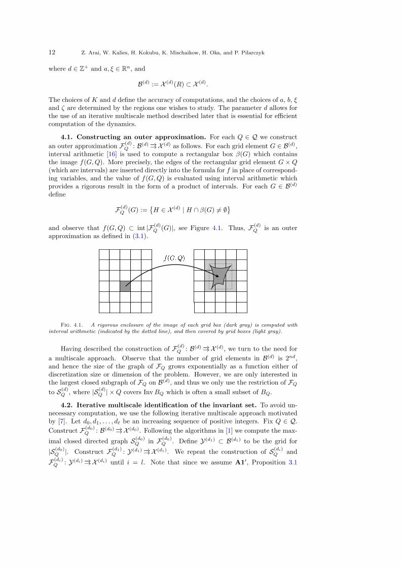
Fig. 4.1. A rigorous enclosure of the image of each grid box (dark gray) is computed withinterval arithmetic (indicated by the dotted line), and then covered by grid boxes (light gray).
Having described the construction of F (d)Q : B(d)−→→X (d), we turn to the need for
a multiscale approach. Observe that the number of grid elements in B(d) is 2nd,and hence the size of the graph of FQ grows exponentially as a function either ofdiscretization size or dimension of the problem. However, we are only interested inthe largest closed subgraph of FQ on B(d), and thus we only use the restriction of FQto S(d)
Q , where |S(d)Q | ×Q covers InvBQ which is often a small subset of BQ.
4.2. Iterative multiscale identification of the invariant set. To avoid un-necessary computation, we use the following iterative multiscale approach motivatedby [7]. Let d0, d1, . . . , d` be an increasing sequence of positive integers. Fix Q ∈ Q.
Construct F (d0)Q : B(d0)−→→X (d0). Following the algorithms in [1] we compute the max-
imal closed directed graph S(d0)Q in F (d0)
Q . Define Y(d1) ⊂ B(d1) to be the grid for
|S(d0)Q |. Construct F (d1)
Q : Y(d1)−→→X (d1). We repeat the construction of S(di)Q and
F (di)Q : Y(di)−→→X (di) until i = l. Note that since we assume A1′, Proposition 3.1
A Database Schema for the Analysis of Global Dynamics of Multiparameter Systems 13
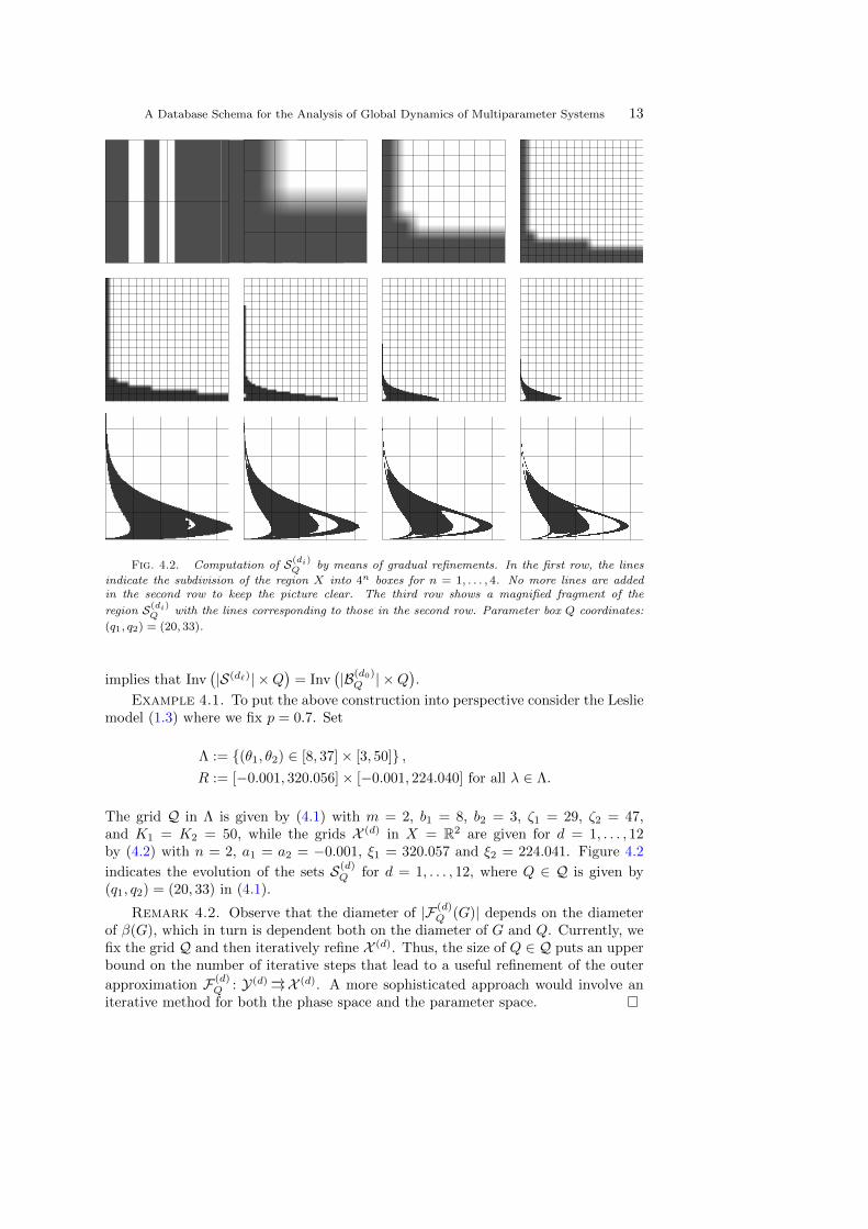
Fig. 4.2. Computation of S(di)Q by means of gradual refinements. In the first row, the lines
indicate the subdivision of the region X into 4n boxes for n = 1, . . . , 4. No more lines are addedin the second row to keep the picture clear. The third row shows a magnified fragment of the
region S(di)Q with the lines corresponding to those in the second row. Parameter box Q coordinates:
(q1, q2) = (20, 33).
implies that Inv(|S(d`)| ×Q
)= Inv
(|B(d0)Q | ×Q
).
Example 4.1. To put the above construction into perspective consider the Lesliemodel (1.3) where we fix p = 0.7. Set
Λ := (θ1, θ2) ∈ [8, 37]× [3, 50] ,R := [−0.001, 320.056]× [−0.001, 224.040] for all λ ∈ Λ.
The grid Q in Λ is given by (4.1) with m = 2, b1 = 8, b2 = 3, ζ1 = 29, ζ2 = 47,and K1 = K2 = 50, while the grids X (d) in X = R2 are given for d = 1, . . . , 12by (4.2) with n = 2, a1 = a2 = −0.001, ξ1 = 320.057 and ξ2 = 224.041. Figure 4.2
indicates the evolution of the sets S(d)Q for d = 1, . . . , 12, where Q ∈ Q is given by
(q1, q2) = (20, 33) in (4.1).
Remark 4.2. Observe that the diameter of |F (d)Q (G)| depends on the diameter
of β(G), which in turn is dependent both on the diameter of G and Q. Currently, wefix the grid Q and then iteratively refine X (d). Thus, the size of Q ∈ Q puts an upperbound on the number of iterative steps that lead to a useful refinement of the outer
approximation F (d)Q : Y(d)−→→X (d). A more sophisticated approach would involve an
iterative method for both the phase space and the parameter space.
14 Z. Arai, W. Kalies, H. Kokubu, K. Mischaikow, H. Oka, and P. Pilarczyk
Remark 4.3. By Proposition 3.1, SQ ⊂ |S(di)Q | × Q for i = 0, . . . , l. Moreover,
since S(di)Q is the maximal closed subgraph, and combinatorial Morse sets are closed
subgraphs, each combinatorial Morse set MQ(p) for p ∈ PQ is contained in S(di)Q for
each i = 0, . . . , `. If F(MQ(p)
)⊂ BQ for all p ∈ PQ, then by Proposition 3.2, the
neighborhoods |MQ(p)| isolate Morse sets in a Morse decomposition of SQ. Moreover,since Morse sets are recurrent, the condition F
(MQ(p)
)⊂ BQ implies that
FQ(FQ(MQ(p)) \MQ(p)
)∩MQ(p) = ∅, (4.3)
where FQ : X → X is an outer approximation. As described in the next section,this allows us to readily compute the Conley index of Inv (|MQ|). If the conditionF(MQ(p)
)⊂ BQ is not satisfied, then we cannot compute the index without extend-
ing our computation of FQ outside of BQ, and this situation is reported in the outputof our computations.
4.3. Conley-Morse graph computation. Given F (d`)Q : S(d`)
Q−→→X (d`) the al-
gorithm in [1, Section 2.2] is used to compute the Morse graph MG(FQ), where
FQ := F (d`)Q . To produce the Conley-Morse graph over Q requires the computa-
tion of the Conley indices of each Morse set. This is done using the algorithms in[14, 20] and the easy observation that if MQ(p) is a combinatorial Morse set forFQ and the condition (4.3) is satisfied for FQ : MQ(p) ∪ FQ(MQ(p))−→→X , then(MQ(p)∪FQ(MQ(p)), FQ(MQ(p)) \MQ(p)
)is a combinatorial index pair as in
[19, 20]. In practice, there are memory constraints associated with these algorithmsfor computing the Conley index. In the computations performed for this paper wedid not attempt to compute the Conley index if the index pairs generated containedmore than 400,000 boxes.
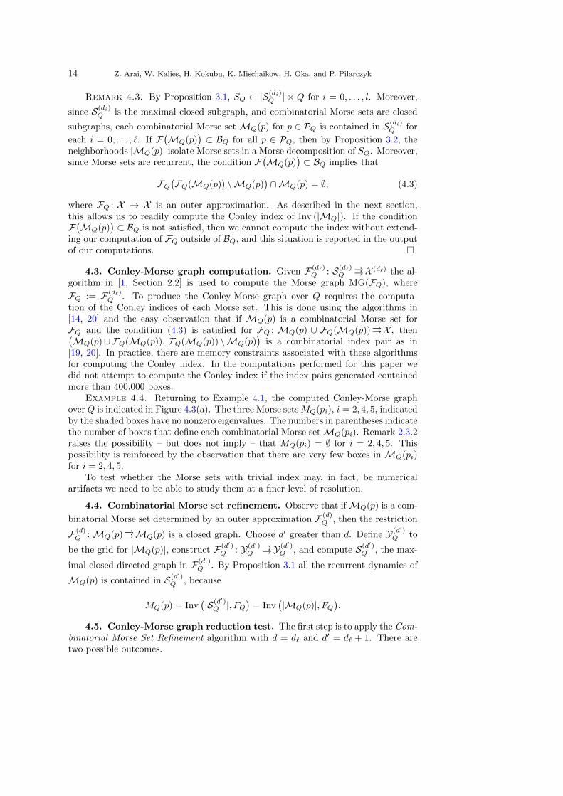
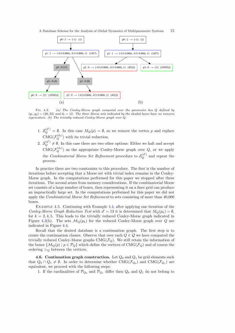
Example 4.4. Returning to Example 4.1, the computed Conley-Morse graphoverQ is indicated in Figure 4.3(a). The three Morse setsMQ(pi), i = 2, 4, 5, indicatedby the shaded boxes have no nonzero eigenvalues. The numbers in parentheses indicatethe number of boxes that define each combinatorial Morse setMQ(pi). Remark 2.3.2raises the possibility – but does not imply – that MQ(pi) = ∅ for i = 2, 4, 5. Thispossibility is reinforced by the observation that there are very few boxes in MQ(pi)for i = 2, 4, 5.
To test whether the Morse sets with trivial index may, in fact, be numericalartifacts we need to be able to study them at a finer level of resolution.
4.4. Combinatorial Morse set refinement. Observe that ifMQ(p) is a com-
binatorial Morse set determined by an outer approximation F (d)Q , then the restriction
F (d)Q : MQ(p)−→→MQ(p) is a closed graph. Choose d′ greater than d. Define Y(d′)
Q to
be the grid for |MQ(p)|, construct F (d′)Q : Y(d′)
Q−→→Y(d′)
Q , and compute S(d′)Q , the max-
imal closed directed graph in F (d′)Q . By Proposition 3.1 all the recurrent dynamics of
MQ(p) is contained in S(d′)Q , because
MQ(p) = Inv(|S(d′)Q |, FQ
)= Inv
(|MQ(p)|, FQ
).
4.5. Conley-Morse graph reduction test. The first step is to apply the Com-binatorial Morse Set Refinement algorithm with d = d` and d′ = d` + 1. There aretwo possible outcomes.
A Database Schema for the Analysis of Global Dynamics of Multiparameter Systems 15
p0 : 2 -1 (1)
p1 : 1 -0.5-0.866i, -0.5+0.866i, 1 (1457)
p4 : 0 (11)
p2 : 0 (8)
p3 : 0 -0.5-0.866i, -0.5+0.866i, 1 (4522)p6 : 0 1 (105052)
p5 : 0 (4)
(a)
p0 : 2 -1 (1)
p1 : 1 -0.5-0.866i, -0.5+0.866i, 1 (1457)
p2 : 0 -0.5-0.866i, -0.5+0.866i, 1 (4522) p3 : 0 1 (105052)
(b)
Fig. 4.3. (a) The Conley-Morse graph computed over the parameter box Q defined by(q1, q2) = (20, 33) and d` = 12. The three Morse sets indicated by the shaded boxes have no nonzeroeigenvalues. (b) The trivially reduced Conley-Morse graph over Q.
1. S(d′)Q = ∅. In this case MQ(p) = ∅, so we remove the vertex p and replace
CMG(F (d`)Q ) with its trivial reduction.
2. S(d′)Q 6= ∅. In this case there are two other options: Either we halt and accept
CMG(F (d`)Q ) as the appropriate Conley-Morse graph over Q, or we apply
the Combinatorial Morse Set Refinement procedure to S(d′)Q and repeat the
process.
In practice there are two constraints to this procedure. The first is the number ofiterations before accepting that a Morse set with trivial index remains in the Conley-Morse graph. In the computations performed for this paper we stopped after threeiterations. The second arises from memory considerations. If the combinatorial Morseset consists of a large number of boxes, then representing it on a finer grid can producean impractically large set. In the computations performed for this paper we did notapply the Combinatorial Morse Set Refinement to sets consisting of more than 40,000boxes.
Example 4.5. Continuing with Example 4.4, after applying one iteration of theConley-Morse Graph Reduction Test with d′ = 13 it is determined that MQ(pk) = ∅,for k = 2, 4, 5. This leads to the trivially reduced Conley-Morse graph indicated inFigure 4.3(b). The sets MQ(pk) for the reduced Conley-Morse graph over Q areindicated in Figure 4.4.
Recall that the desired database is a continuation graph. The first step is tocreate the continuation classes. Observe that over each Q ∈ Q we have computed thetrivially reduced Conley-Morse graphs CMG(FQ). We still retain the information ofthe boxes MQ(p) | p ∈ PQ which define the vertices of CMG(FQ) and of course theordering >Q between the vertices.
4.6. Continuation graph construction. Let Q0 and Q1 be grid elements suchthat Q0 ∩ Q1 6= ∅. In order to determine whether CMG(FQ0) and CMG(FQ1) areequivalent, we proceed with the following steps:
1. If the cardinalities of PQ0 and PQ1 differ then Q0 and Q1 do not belong to

16 Z. Arai, W. Kalies, H. Kokubu, K. Mischaikow, H. Oka, and P. Pilarczyk
Fig. 4.4. The sets MQ(pi), i = 0, 1, 2, 3, for the reduced Conley-Morse graph from Fig-ure 4.3(b). The color coding in the two figures match, thus the green and red regions indicateattracting neighborhoods for fλ for all λ in the parameter box Q defined by (q1, q2) = (20, 33) andd` = 12. The set MQ(p0) covers the origin and consists of a single box at the lower left corner ofthe picture and is barely visible at this resolution.
the same continuation class.2. If the cardinalities of PQ0 and PQ1 agree, then we construct the clutching
graph (see comment preceding Definition 3.5). If the clutching graph de-fines a directed graph isomorphism between the Morse graphs MG(FQ0
) andMG(FQ1
), then the Conley-Morse graphs CMG(FQ0) and CMG(FQ1
) overQ0 and Q1 belong to the same continuation class.
3. The clutching graph can fail to define a directed graph isomorphism betweenthe Morse graphs MG(FQ0) and MG(FQ1) in several ways:• The partial orders do not agree, in which case CMG(FQ0
) and CMG(FQ1)
are not identified as belonging to the same continuation class.• There is a vertex with no edge in the clutching graph, in which case
CMG(FQ0) and CMG(FQ1
) do not belong to the same continuationclass.
• There is a vertex with two or more edges in the clutching graph. Recallthat the edge (p, q) is in the clutching graph if MQ0
(p) ∩MQ1(q) 6= ∅.
Assume the edges at the vertex p are given by (p, qi) | i = 1, . . . , I.Then we apply several iterations of the Combinatorial Morse Set Refine-ment algorithm toMQ0(p) andMQ1(qi), i = 1, . . . , I. If after perform-ing this at each vertex for which there are multiple edges, the clutchinggraph reduces to a directed graph isomorphism, then CMG(FQ0
) and
A Database Schema for the Analysis of Global Dynamics of Multiparameter Systems 17
CMG(FQ1) belong to the same continuation class; otherwise CMG(FQ0
)and CMG(FQ1
) belong to different continuation classes.This procedure applied to all pairs of adjacent boxes in the parameter space
results in the set of continuation classes and the continuation graph which definesthe database having been determined. Note that although this procedure admits thesituation in which two Conley-Morse graphs are identified as belonging to the samecontinuation class even if the clutching function does not define a directed graphisomorphism, in such a case the conclusion of Proposition 3.7 still holds true, becausethe clutching function of the refined combinatorial Morse decompositions does providethe isomorphism.
5. Database for the Leslie model with p = 0.7. In this section we presentthe results of the computational procedure described in Section 4 applied to thedensity dependent Leslie model (1.3) when p = 0.7. The procedure was implementedin an efficient program written in C++. An interactive presentation of the results ofcomputations which we did can be found at http://chomp.rutgers.edu/database/,and the source code of the general purpose software used to compute this databasehas also been made freely available.
Observe that fixing p = 0.7 results in a two-dimensional parameter space. Wecompute the continuation graph over the parameter space
Λ := (θ1, θ2) ∈ [8, 37]× [3, 50] .
We choose an equipartitioned 50 × 50 grid for this parameter space given by (4.1)with m = 2, b1 = 8, b2 = 3, ζ1 = 29, ζ2 = 47, and K1 = K2 = 50.
Recasting the Leslie model in the general form of (1.2) and recalling that x1 andx2 represent population sizes, we are interested in studying F : (R+)2×Λ→ (R+)2×Λwhere R+ := [0,∞).
There are two essential observations.Remark 5.1. For λ = (θ1, θ2), define
Bλ :=
(x1, x2) ∈ (R+)2 | 0 ≤ x1 ≤ 10(θ1 + θ2)e−1, 0 ≤ x2 ≤ 10p(θ1 + θ2)e−1.
A direct calculation shows that F 2((R+)2×Λ
)⊂ B :=
⋃λ∈ΛBλ×λ. In particular,
any invariant set for the Leslie model on (R+)2 must lie in B. Furthermore, F (0, λ) =(0, λ) and 0 × (0,∞) 6⊂ fλ
((R+)2
).
Remark 5.2. There are some technical reasons why we do not compute on theset B ⊂ (R+)2 × Λ as defined in Remark 5.1. First, F (0, λ) = (0, λ) so that B isnot an isolating neighborhood as a subset of R2 × Λ. While this would not violateA1 restricted to (R+)2 × Λ, it does imply that the Conley index of the invariant set0 computed restricted to B would not be capable of measuring the hyperbolicity ofthe origin. Our approach to this problem is pragmatic, we can explicitly compute theeigenvalues at the origin as
µ± =θ1 ±
√θ2
1 + 4pθ2
2.
Observe that restricted to Λ, µ+ > 1. This information can then be used to computethe index analytically. However, this is not the only reason not to compute on B.
As exhibited in the figures in the next section, the maximal invariant set in Bcomes very close to the coordinate axes, even though it does not touch the axes by
18 Z. Arai, W. Kalies, H. Kokubu, K. Mischaikow, H. Oka, and P. Pilarczyk
Remark 5.1. This causes a problem again in isolating and computing the Conley indexeven for some Morse sets that do not include the origin, when the computations arerestricted to the first quadrant.
Given these issues, we have chosen to compute on a larger rectangle
R := [−0.001, 320.056]× [−0.001, 224.040]
in R2 and consider the origin analytically. With respect to the dynamics on R2, theorigin undergoes a period doubling bifurcation since µ− < −1 if θ2 >
1pθ1 + 1 and
−1 < µ− < 0 if θ2 <1pθ1 + 1. The eigenvector v+ associated with µ+ can be chosen
to lie in the positive orthant. The eigenvector associated with µ− lies outside thepositive cone. Thus, this period doubling bifurcation has no direct impact on theordering of the Morse decomposition of Sλ := Inv (R, fλ). Combining this with theobservation that µ+ > 1, one can conclude that for any λ ∈ Λ the origin is always arepeller for Sλ.
These observations imply that, even though the condition A1′ does not hold nearthe period-doubling bifurcation, this bifurcation plays no role in the constructionof the continuation classes. Moreover, the Conley index of the origin provides noinformation, and hence can be ignored in the database.
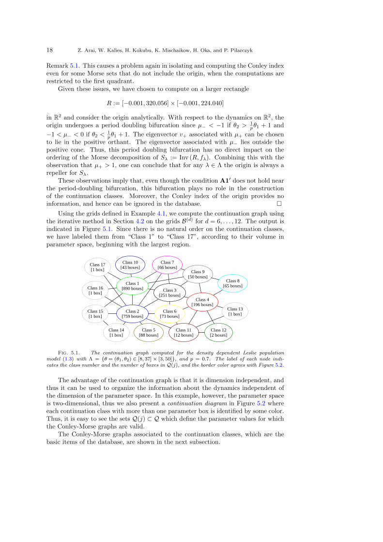
Using the grids defined in Example 4.1, we compute the continuation graph usingthe iterative method in Section 4.2 on the grids B(d) for d = 6, . . . , 12. The output isindicated in Figure 5.1. Since there is no natural order on the continuation classes,we have labeled them from “Class 1” to “Class 17”, according to their volume inparameter space, beginning with the largest region.
Class 1[890 boxes]
Class 2[759 boxes]
Class 3[251 boxes]
Class 4[196 boxes]
Class 5[88 boxes]
Class 6[73 boxes]
Class 7[66 boxes]
Class 8[65 boxes]
Class 9[50 boxes]
Class 10[43 boxes]
Class 11[12 boxes]
Class 12[2 boxes]
Class 13[1 box]
Class 14[1 box]
Class 15[1 box]
Class 16[1 box]
Class 17[1 box]
Fig. 5.1. The continuation graph computed for the density dependent Leslie populationmodel (1.3) with Λ = θ = (θ1, θ2) ∈ [8, 37]× [3, 50], and p = 0.7. The label of each node indi-cates the class number and the number of boxes in Q(j), and the border color agrees with Figure 5.2.
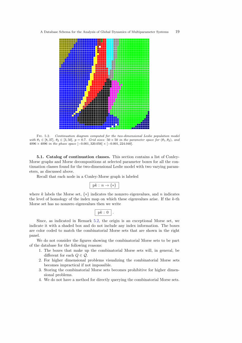
The advantage of the continuation graph is that it is dimension independent, andthus it can be used to organize the information about the dynamics independent ofthe dimension of the parameter space. In this example, however, the parameter spaceis two-dimensional, thus we also present a continuation diagram in Figure 5.2 whereeach continuation class with more than one parameter box is identified by some color.Thus, it is easy to see the sets Q(j) ⊂ Q which define the parameter values for whichthe Conley-Morse graphs are valid.
The Conley-Morse graphs associated to the continuation classes, which are thebasic items of the database, are shown in the next subsection.
A Database Schema for the Analysis of Global Dynamics of Multiparameter Systems 19
Fig. 5.2. Continuation diagram computed for the two-dimensional Leslie population modelwith θ1 ∈ [8, 37], θ2 ∈ [3, 50], p = 0.7. Grid sizes: 50 × 50 in the parameter space for (θ1, θ2), and4096× 4096 in the phase space [−0.001, 320.056]× [−0.001, 224.040].
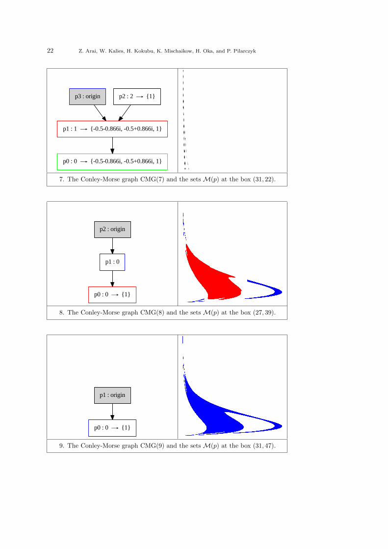
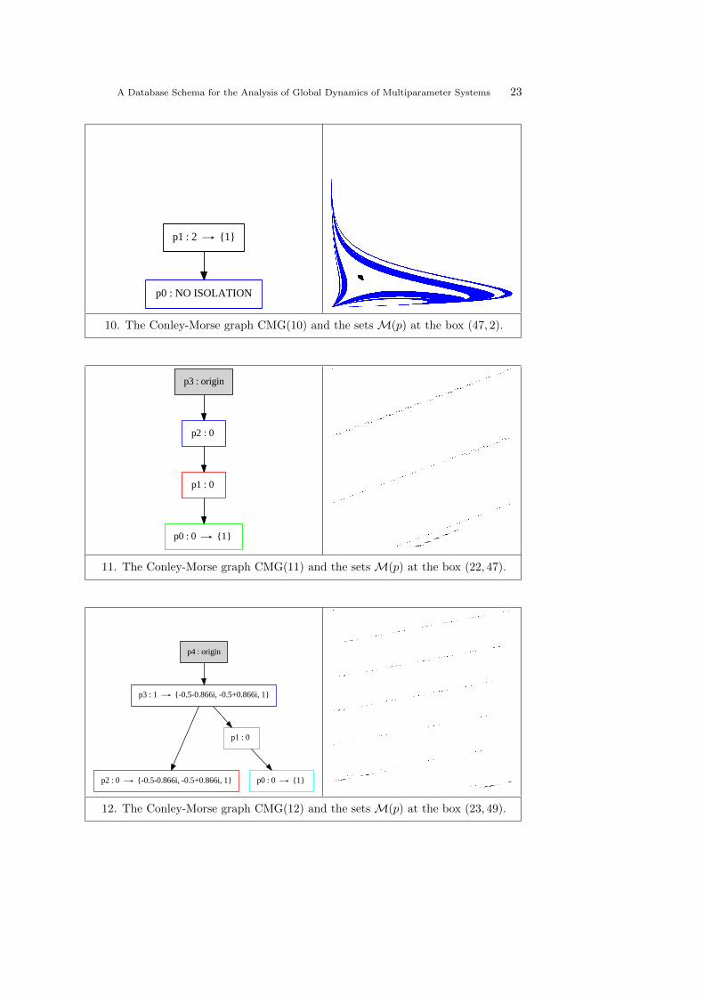
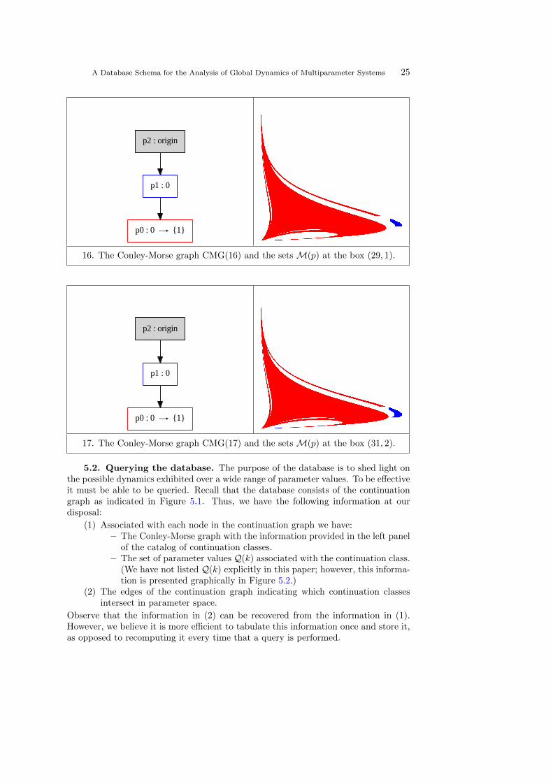
5.1. Catalog of continuation classes. This section contains a list of Conley-Morse graphs and Morse decompositions at selected parameter boxes for all the con-tinuation classes found for the two-dimensional Leslie model with two varying param-eters, as discussed above.
Recall that each node in a Conley-Morse graph is labeled
pk : n→ ∗
where k labels the Morse set, ∗ indicates the nonzero eigenvalues, and n indicatesthe level of homology of the index map on which these eigenvalues arise. If the k-thMorse set has no nonzero eigenvalues then we write
pk : 0 .
Since, as indicated in Remark 5.2, the origin is an exceptional Morse set, weindicate it with a shaded box and do not include any index information. The boxesare color coded to match the combinatorial Morse sets that are shown in the rightpanel.
We do not consider the figures showing the combinatorial Morse sets to be partof the database for the following reasons:
1. The boxes that make up the combinatorial Morse sets will, in general, bedifferent for each Q ∈ Q.
2. For higher dimensional problems visualizing the combinatorial Morse setsbecomes impractical if not impossible.
3. Storing the combinatorial Morse sets becomes prohibitive for higher dimen-sional problems.
4. We do not have a method for directly querying the combinatorial Morse sets.
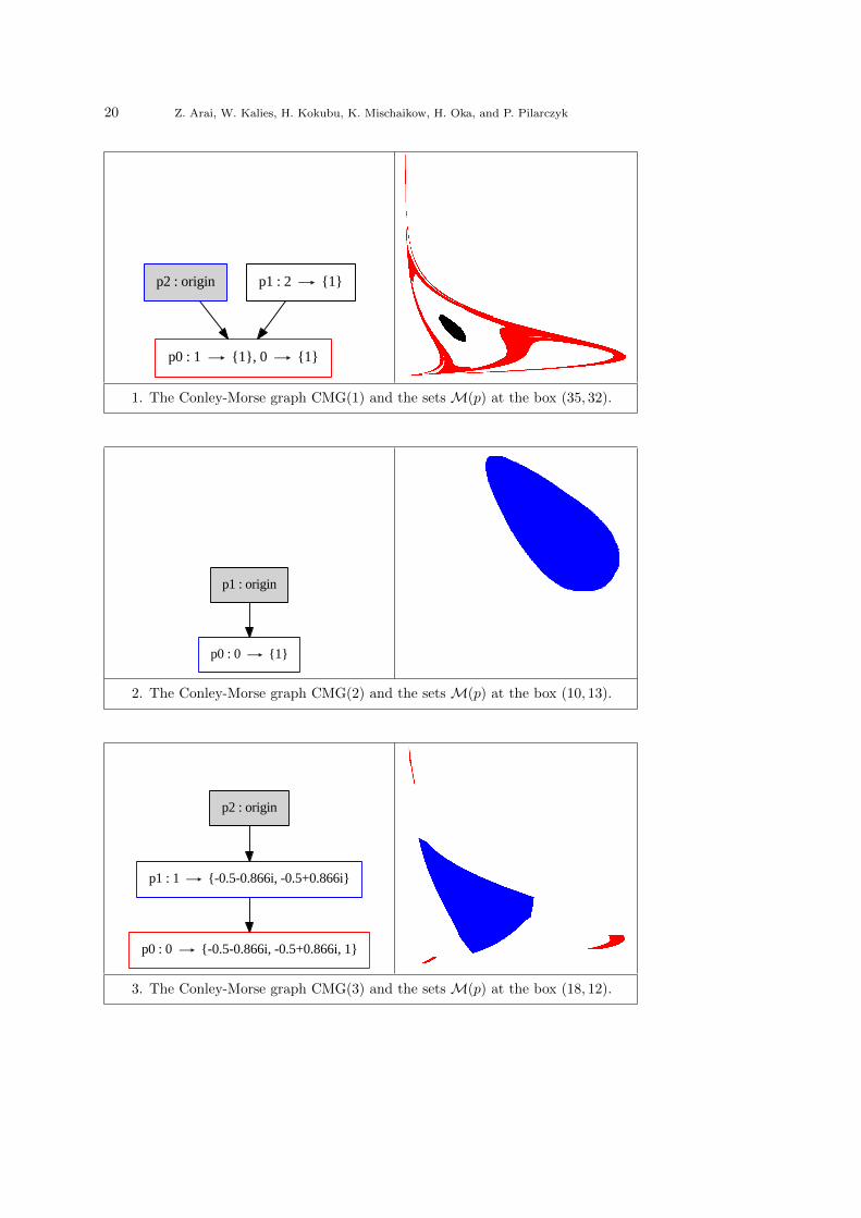
20 Z. Arai, W. Kalies, H. Kokubu, K. Mischaikow, H. Oka, and P. Pilarczyk
p2 : origin
p0 : 1 1, 0 1
p1 : 2 1
1. The Conley-Morse graph CMG(1) and the sets M(p) at the box (35, 32).
p1 : origin
p0 : 0 1
2. The Conley-Morse graph CMG(2) and the sets M(p) at the box (10, 13).
p2 : origin
p1 : 1 -0.5-0.866i, -0.5+0.866i
p0 : 0 -0.5-0.866i, -0.5+0.866i, 1
3. The Conley-Morse graph CMG(3) and the sets M(p) at the box (18, 12).
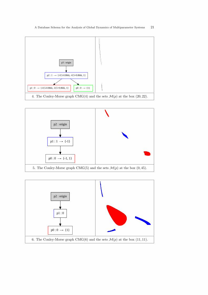
A Database Schema for the Analysis of Global Dynamics of Multiparameter Systems 21
p3 : origin
p2 : 1 -0.5-0.866i, -0.5+0.866i, 1
p1 : 0 -0.5-0.866i, -0.5+0.866i, 1 p0 : 0 1
4. The Conley-Morse graph CMG(4) and the sets M(p) at the box (20, 22).
p2 : origin
p1 : 1 -1
p0 : 0 -1, 1
5. The Conley-Morse graph CMG(5) and the sets M(p) at the box (0, 45).
p2 : origin
p1 : 0
p0 : 0 1
6. The Conley-Morse graph CMG(6) and the sets M(p) at the box (11, 11).
22 Z. Arai, W. Kalies, H. Kokubu, K. Mischaikow, H. Oka, and P. Pilarczyk
p3 : origin
p1 : 1 -0.5-0.866i, -0.5+0.866i, 1
p2 : 2 1
p0 : 0 -0.5-0.866i, -0.5+0.866i, 1
7. The Conley-Morse graph CMG(7) and the sets M(p) at the box (31, 22).
p2 : origin
p1 : 0
p0 : 0 1
8. The Conley-Morse graph CMG(8) and the sets M(p) at the box (27, 39).
p1 : origin
p0 : 0 1
9. The Conley-Morse graph CMG(9) and the sets M(p) at the box (31, 47).
A Database Schema for the Analysis of Global Dynamics of Multiparameter Systems 23
p1 : 2 1
p0 : NO ISOLATION
10. The Conley-Morse graph CMG(10) and the sets M(p) at the box (47, 2).
p3 : origin
p2 : 0
p1 : 0
p0 : 0 1
11. The Conley-Morse graph CMG(11) and the sets M(p) at the box (22, 47).
p4 : origin
p3 : 1 -0.5-0.866i, -0.5+0.866i, 1
p2 : 0 -0.5-0.866i, -0.5+0.866i, 1
p1 : 0
p0 : 0 1
12. The Conley-Morse graph CMG(12) and the sets M(p) at the box (23, 49).
24 Z. Arai, W. Kalies, H. Kokubu, K. Mischaikow, H. Oka, and P. Pilarczyk
p4 : origin
p3 : 1 -0.5-0.866i, -0.5+0.866i, 1
p2 : 0 -0.5-0.866i, -0.5+0.866i, 1
p1 : 0
p0 : 0 1
13. The Conley-Morse graph CMG(13) and the sets M(p) at the box (22, 45).
p2 : origin
p1 : 0
p0 : 0 1
14. The Conley-Morse graph CMG(14) and the sets M(p) at the box (26, 0).
p3 : origin
p1 : 0 p2 : 2 1
p0 : 1 1, 0 1
15. The Conley-Morse graph CMG(15) and the sets M(p) at the box (27, 0).
A Database Schema for the Analysis of Global Dynamics of Multiparameter Systems 25
p2 : origin
p1 : 0
p0 : 0 1
16. The Conley-Morse graph CMG(16) and the sets M(p) at the box (29, 1).
p2 : origin
p1 : 0
p0 : 0 1
17. The Conley-Morse graph CMG(17) and the sets M(p) at the box (31, 2).
5.2. Querying the database. The purpose of the database is to shed light onthe possible dynamics exhibited over a wide range of parameter values. To be effectiveit must be able to be queried. Recall that the database consists of the continuationgraph as indicated in Figure 5.1. Thus, we have the following information at ourdisposal:
(1) Associated with each node in the continuation graph we have:– The Conley-Morse graph with the information provided in the left panel
of the catalog of continuation classes.– The set of parameter values Q(k) associated with the continuation class.
(We have not listed Q(k) explicitly in this paper; however, this informa-tion is presented graphically in Figure 5.2.)
(2) The edges of the continuation graph indicating which continuation classesintersect in parameter space.
Observe that the information in (2) can be recovered from the information in (1).However, we believe it is more efficient to tabulate this information once and store it,as opposed to recomputing it every time that a query is performed.
26 Z. Arai, W. Kalies, H. Kokubu, K. Mischaikow, H. Oka, and P. Pilarczyk
The reader should also observe that this database is reasonably small. The con-tinuation graph has 17 nodes and 33 edges. Each node contains a directed graph, butthese directed graphs typically only have 3 or 4 nodes and edges. Thus, memory isnot an issue with regard to storage of the database, and queries of the database arefast. For the remainder of this section we demonstrate how the database can be usedto answer relevant questions about the dynamics of the Leslie model.
5.2.1. Multiple basins of attraction. A fundamental question for any dy-namical system is whether there exist multiple basins of attraction. Our ability todetect basins of attraction is based on the following proposition which follows fromthe fact that FQ is an outer approximation [9].
Proposition 5.3. Assume A1. Furthermore, assume that S is a global attractorfor F . Let MQ(p) | p ∈ PQ be the set of combinatorial Morse sets for FQ. If q isminimal with respect to the order >Q, that is, q 6> p for all p ∈ PQ, then M(q) is atrapping region for FQ.
With regard to the density dependent Leslie model, Remark 5.1 implies that S isthe global attractor for the dynamics restricted to (R+)2. Therefore, the existence ofmultiple disjoint trapping regions in (R+)2 implies the existence of multiple distinctbasins of attraction. Thus the following query identifies regions in parameter spacewhich support multiple basins of attraction.
Which continuation classes have a Conley-Morse graph with morethan one minimal element?
The result of this query is Q(k) : k = 4, 12, 13, and each of the graphs has
two minimal elements. Thus Q :=⋃k=4,12,13Q(k) is a region in parameter space for
which there exist at least two basins of attraction. From the edges of the connectiongraph we see that this defines a connected region (we can compute the homology of
Q to conclude that it is contractible). Furthermore, there are 199 boxes in Q, whichrepresents approximately 8% of parameter space.
Remark 5.4. If we define Λ ⊂ Λ to be the set of parameter values at whichfλ possesses multiple basins of attraction, then |Q| ⊂ int (Λ). The inclusion follows
from the fact that Q is determined by the outer approximation F and thus if theattractors are too close together then they cannot be separated by F . However, giventhat in applications (1.3) is meant to represent a biological population, one wouldexpect noise in the system. Depending on the variance in the noise and the errorbounds associated with F , it is possible that |Q| is a more appropriate measure of the
experimentally observable attractors than Λ.
5.2.2. Persistence. The notion of persistence was introduced to account for thefact that though a population model, such as the density dependent Leslie model, isdeterministic and predicts that it is impossible to have extinction, in practice popu-lations are subject to stochastic perturbations. For a biologically motivated reviewsee [22], wherein the following three notions of persistence are discussed. We recastthese definitions to be specifically directed towards the Leslie model considered here.Recall the sets Bλ for λ = (θ1, θ2) defined in Remark 5.1, and further define
Bλ :=
(x1, x2) ∈ (R+)2 | 0 < x1 ≤ 10(θ1 + θ2)e−1, 0 < x2 ≤ 10p(θ1 + θ2)e−1
.
1. f is persistent despite frequent small perturbations if there exists a state x ∈Bλ
and ε > 0 such that there are no ε-chains from x to 0.
A Database Schema for the Analysis of Global Dynamics of Multiparameter Systems 27
2. f is persistent despite rare large perturbations if the origin is not in the closure
of⋃ω(x) | x ∈
Bλ.
3. f is robustly persistent despite frequent small perturbations (respectively, ro-bustly persistent despite rare large perturbations) if all maps g sufficiently nearf are persistent despite frequent small perturbations (respectively, persistentdespite rare large perturbations).
It is easy to check that f2(Bλ, λ) ⊂Bλ ∪0. Furthermore, by Remark 5.2 for
the parameter range Λ covered by the database, the origin is always unstable, andthus for each λ ∈ Λ the Leslie model satisfies all these notions of persistence (if oneconsiders C1 perturbations of the model).
This statement is no longer true, however, if one fixes the size of the allowedperturbations. This can be seen from the database via the following query:
Which continuation classes have a Conley-Morse graph CMG(k) inwhich the box G containing the origin belongs to a combinatorialMorse set M(p) which is a minimal element of CMG(k)?
Observe that for CMG(10) the minimal Morse set is shaded indicating that the boxcontaining the origin belongs to M(0). Observe that Q(10) contains 43 boxes ofparameter space and is in the region of the parameter space Λ corresponding to largevalues of seed production of the first age class.
5.2.3. Cycle sets. One of the goals of population dynamics is to explain fluc-tuations in population levels. We now explain how the database can be used for thispurpose. As indicated in Section 2.2, the Conley index can be used to understandthe structure of the dynamics within a Morse set. For a more complete descriptionof how this can be done the reader is referred to [8, 13]. Here we concentrate on theexistence of equilibria and periodic orbits. We begin by stating the following result(see [8, 13]).
Proposition 5.5. Let f : Rn → Rn be continuous. If K is a hyperbolic periodicorbit of f with minimal period τ ∈ N and unstable manifold of dimension d, then theset of nonzero eigenvalues of the index map occur on the d-th homology groups andare:
eithere2πinτ | n = 0, . . . , τ − 1
or
−e2πinτ | n = 0, . . . , τ − 1
.
The first case occurs if the action on the unstable manifold is orientation preservingand the second case occurs if the action is orientation reversing.
Remark 5.6. The converse of Proposition 5.5 need not be true. A simplecounterexample can be found by considering the logistic equation fλ(x) = λx(1− x)for λ ≈ 3.0 and the isolating neighborhood N = [0.6, 0.7]. For λ < 3.0, the maximalinvariant set is a unique stable hyperbolic fixed point and thus the nonzero eigenvaluesare 1 on the 0-th homology group. However, for λ > 3.0 the maximal invariant setcontains an unstable fixed point, a stable periodic orbit of period two, and a connectingorbit from the fixed point to the periodic orbit. Consider, however, the logistic mapas a population model with a small amount of noise. At parameter values λ ≈ 3.0, anobserver would detect that orbits converge to the neighborhood N , but would not beable to distinguish the existence of the period two orbit. Thus, from the point of viewof an experimentalist, it is conceivable that it is more useful to identify the invariantset inside N with a fixed point. This leads us to the following definition.
Definition 5.7. Let g : Z → Z be a continuous map. An isolated invariantset S is a T -cycle set if there exist T disjoint, compact regions N1, . . . , NT such that
28 Z. Arai, W. Kalies, H. Kokubu, K. Mischaikow, H. Oka, and P. Pilarczyk
S = Inv (N, g), where N :=⋃Ti=1Ni is an isolating neighborhood, and
g(Ni) ∩N ⊂ Ni+1, i = 0, . . . T − 1,
where N0 = NT . Moreover, S is an attracting T -cycle set if g(Ni) ⊂ Ni+1 for i =0, . . . , T − 1.
Heuristically the dynamics associated with a T -cycle set could resemble that of aperiodic orbit with minimal period T , but subject to perturbations.
Proposition 5.8. LetMQ be a combinatorial Morse set obtained using a rectan-gular grid on the phase space. Let MQ = Inv
(|MQ|, FQ
). Then the set of nontrivial
eigenvalues of the index map on the 0-th level of homology is
either ∅ ore2πi kT | k = 0, . . . , T − 1
.
In the latter case, MQ is an attracting T -cycle set.Proof. Since |MQ| is an isolating block [9], the work of [18] implies that there
exists an index pair for FQ of the form P = (P1, P0) where P1 = |MQ|.Let MQ =
⋃Jj=1Nj where |Nj | are the disjoint components of P1. Let J =
1, . . . , J. Let I = j ∈ J | |Nj | ∩ P0 = ∅. Observe that
H0(N1, N0) ∼=⊕j∈J
H0
(|Nj |, |Nj | ∩ P0
) ∼= ⊕j∈I
H0
(|Nj |, |Nj | ∩ P0
) ∼= ⊕j∈I
Z[ξj ],
where ξj is the generator of H0
(|Nj |, |Nj | ∩ P0
).
Consider j ∈ I. Since (P1, P0) is an index pair and |Nj | has no exit set associatedwith it, this implies that FQ
(|Nj |
)⊂ |N`| for some ` ∈ J . If ` ∈ I, then FQP∗(ξj) =
ξ`. If ` 6∈ I, then FQP∗(ξj) = 0.SinceMQ is a combinatorial Morse set, it is an equivalence class of the recurrent
set. Thus, if I 6= J , then FQ∗ is nilpotent on the 0-th level. In this case the setof nonzero eigenvalues is ∅. If I = J , then FQP∗ restricted to the 0-th level is apermutation matrix and the associated eigenvalues are roots of unit with T = J .
This remark leads us to propose the following query for identifying attractingcyclic sets.
For a fixed τ ∈ 1, 2, 3, . . ., which continuation classes have a Conley-Morse graph whose minimal node has nonzero eigenvalues
e2πinτ |
n = 0, . . . , τ − 1
at the 0-th homology level?
The result of this query indicates that there is an attracting 1-cycle set for theparameter values Q(k), k = 1, 2, 4, 6, 8, 9, 11, 12, 13, 14, 16, 17, an attracting 2-cycle setat Q(k), k = 5, and an attracting 3-cycle set at Q(k), k = 3, 4, 7, 12, 13, 15.
Observe that this analysis also provides us with a better understanding of thepossible dynamics at those parameter values where we identified multiple basins ofattraction Q(k), k = 4, 12, 13. A T -cycle set is a very weak description of the dynam-ics. Careful numerical studies such as those of [25] suggest the existence of chaoticdynamics at some of the parameter values associated with the 3-cycle sets. Some ofthis finer information can be also obtained using the Conley index. For example, each2-cycle and 3-cycle set contains a period 2 and period 3 orbit, respectively (thoughthese orbits need not be stable). There are also Conley index techniques for extract-ing entropy estimates and symbolic dynamics within Morse sets [11, 23, 5, 4]. The
A Database Schema for the Analysis of Global Dynamics of Multiparameter Systems 29
relevance of this information is problem dependent. However, to extract this infor-mation will require refinements of the current algorithms being used to construct thedatabase.
As discussed in [3], attempting to match the dynamics of a deterministic modelto experimental data in which the presence of noise is to be expected requires anunderstanding of not only the structure of attractors, but also of the unstable invariantsets. This is because with sufficient time stochastic events will almost certainly pushthe trajectory away from the attractors in which case the dynamics will be determinedby the stable and unstable manifolds of the unstable invariant sets. In the context ofthe Leslie model, perhaps the most interesting cases in which to study the unstableinvariant sets is to identify the separatrices in the case of multiple basins of attraction.This is done using the following type of query.
The minimal nodes in CMG(4) are 1, 0. Find the minimal node psuch that p > 1 and p > 0.
The result of this query is MQ(4)(2) for which the nonzero eigenvalues aree2πin3 |
n = 0, 1, 2
which suggests the behavior of a period three orbit with a one-dimensionalorientable unstable manifold.
6. Database for the Leslie model. To some extent Section 5 is included forpedagogical purposes. Our hope is that the continuation diagram, Figure 5.2, andthe fact that there are only 17 continuation classes provides the reader with a clearindication of the potential use and applicability of the database. As discussed in thederivation of (1.3), the density dependent Leslie model involves three parameters.The computational procedures described in Section 4 are dimension independent, andthus we can apply them to (1.3) over the parameter space
Λ := (θ1, θ2, p) ∈ [8, 37]× [3, 50]× [0.5, 0.9] .
We choose an equipartitioned 80 × 80 × 40 grid for this parameter space, given by(4.1) with m = 3, b1 = 8, b2 = 3, b3 = 0.5, ζ1 = 29, ζ2 = 47, ζ3 = 0.4, K1 = K2 = 80,and K3 = 40.
Recasting the Leslie model in the general form of (1.2) and recalling that x1 andx2 represent population sizes, we are interested in studying F : (R+)2×Λ→ (R+)2×Λwhere R+ := [0,∞). Remarks 5.1 and 5.2 are still applicable and thus, as explainedin the previous section, for all parameter values λ ∈ Λ we compute on
R := [−0.001, 320.056]× [−0.001, 288.051]
and the grids X (d) in X = R2 are given for d = 1, 2, . . . by (4.2) with n = 2, a1 =a2 = −0.001, ξ1 = 320.057 and ξ2 = 288.052.
With this input we compute the continuation graph using iteratively generatedgrids X (d) in the phase space for d = 6, . . . , 12.
Using the techniques outlined in Section 4, a continuation graph was computedin 5,225 CPU hours on a cluster based on AMD Opteron 248 processors with 4 GB ofmemory per node. This results in a continuation graph with 92 vertices and 263 edges.Because of the size of the graph its visual presentation is of limited use. Also, since weare working with a three-dimensional parameter space and 256,000 parameter boxes,there is no hope of presenting a continuation diagram in this paper. An attempt hasbeen made at the website http://chomp.rutgers.edu/database/ to use a series oftwo-dimensional pictures of slices of the diagram, either as an animation or as a list
30 Z. Arai, W. Kalies, H. Kokubu, K. Mischaikow, H. Oka, and P. Pilarczyk
of consecutive images, to visualize the continuation diagram; an interested reader iskindly invited to explore these results further. Although careful analysis of this kindof visualization may shed light on the dynamics of interest, we would like to point outthat this approach will not work in higher dimensions, and is therefore of limited use.
Independent of how complicated the continuation graph is, however, the queriesfrom Section 5.2 can still be performed with equal ease and provide the followingresults:
• There are parameter values associated with multiple basins of attraction.– At Q(k), k = 6, 10, 34, 37, 51, 58, 59 (comprising 18,632 boxes in param-
eter space) one attractor is a 1-cycle set and the other attractor is a3-cycle set. The index information suggests (there is no theorem toguarantee this; however, visual inspection confirms this) that the sepa-ratrix between the basins of attraction has the behavior of an unstable3-cycle set.
– At Q(k), k = 15, 17 (comprising 221 boxes in parameter space) oneattractor is a 2-cycle set and the other attractor is a 3-cycle set. Theindex information also suggests that the separatrix between the basinsof attraction has the behavior of an unstable 3-cycle set.
• Persistence is lost on the level of the computational grid for the parametervalues in Q(k), k = 7 (comprising 16,686 boxes in parameter space).
7. Final remarks. The presentation of this paper has focused on discrete timedynamical systems. On a theoretical level it is clear that the same ideas apply todynamics generated by differential equations. In particular, if one considers a param-eterized family of semiflows ϕ : [0,∞) × X × Λ → X and chooses a constant τ > 0,then the time-τ map ϕτ = ϕ(τ, ·, ·) : X × Λ → X returns one to the setting of thispaper. On a practical level the issue is much more subtle. Typically, the semiflow isdefined in terms of solutions to a differential equation. Thus, constructing an outerapproximation requires rigorous numerical calculation of an enclosure of the forwardtranslation of a grid element. There are tools for doing this effectively (see in par-ticular the work of the CAPD group [26]); however, the computational cost is clearlymuch greater than the simple evaluation of a formula as was done in this paper. Fur-thermore, if τ is chosen to be small, then ϕτ represents a perturbation of the identity.In order to identify interesting dynamics in this case, the diameter of the grid onphase space will need to be extremely small. On the other hand, if τ is chosen tobe large, then not only does the cost of evaluation of ϕτ on grid elements becomelarge, growing at least proportionally to τ , but also for a reasonable computationalcost, the error bounds on the images of the grid elements will be extremely large. Animportant open problem is then how to choose, a priori, an appropriate size for τ .
Another obvious topic which has only been briefly discussed is the relationshipbetween the continuation classes and classical bifurcation theory. As was pointedout in Remark 3.8, the boundaries between the continuation classes need not rep-resent boundaries between different topological conjugacy classes of dynamics, andvice versa. Using standard bifurcation analysis it is fairly easy to check that a perioddoubling bifurcation occurs near the boundary between continuation classes 2 and 5(see Figure 5.2). Similarly, a saddle-node bifurcation to a period three orbit occurswithin continuation class 6 as one passes from continuation class 2 to continuationclass 4. However, recognizing these bifurcations from the database and predictinghow the database will represent these bifurcations as a function of grid size in bothphase space and parameter space remains an open problem.
A Database Schema for the Analysis of Global Dynamics of Multiparameter Systems 31
Acknowledgements: The authors thank anonymous referees for their carefulreading of the manuscript and their useful suggestions.
REFERENCES
[1] H. Ban and W. Kalies, A computational approach to Conley’s decomposition theorem, Journalof Computational and Nonlinear Dynamics 1 (2006), pp. 312–319.
[2] C. Conley, Isolated invariant sets and the Morse index, CBMS Regional Conference Series inMathematics Vol. 38, American Mathematical Society, Providence, R.I., 1978.
[3] J. M. Cushing, R. F. Costantino, B. Dennis, R. A. Desharnais, and S. M. Henson, Non-linear population dynamics: Models, experiments and data, J. Theoret. Biol. 194 (1998),pp. 1–9.
[4] S. Day, R. Frongillo, and R. Trevino, Algorithms for Rigorous Entropy Bounds and Sym-bolic Dynamics, SIAM J. Appl. Dyn. Syst., 7 (2008) pp. 1477-1506.
[5] S. Day, O. Junge, and K. Mischaikow, A rigorous numerical method for the global analysisof infinite dimensional discrete dynamical systems, SIAM J. Appl. Dyn. Syst. 3 (2004),pp. 117–160.
[6] M. Dellnitz, G. Froyland, and O. Junge, The algorithms behind GAIO – Set orientednumerical methods for dynamical systems, B. Fiedler (ed.), Ergodic Theory, Analysis, andEfficient Simulation of Dynamical Systems, pp. 145–174, Springer-Verlag, 2001.
[7] M. Dellnitz and A. Hohmann, A subdivision algorithm for the computation of unstable man-ifolds and global attractors, Numer. Math. 75 (1997), pp. 293–317.
[8] T. Kaczynski, K. Mischaikow, and M. Mrozek, Computational homology, volume 157 ofApplied Mathematical Sciences, Springer-Verlag, New York, 2004.
[9] W. D. Kalies, K. Mischaikow, and R. C. A. M. VanderVorst, An algorithmic approach tochain recurrence, Found. Comput. Math. 5 (2005), pp. 409–449.
[10] A. Lander, A calculus of purpose, PLoS Biology 2 (2004), pp. 712–714 (electronic).[11] K. Mischaikow and M. Mrozek, Isolating neighborhoods and chaos, Japan J. Indust. Appl.
Math. 12 (1995), pp. 205–236.[12] K. Mischaikow and M. Mrozek, Chaos in the Lorenz equations: a computer-assisted proof,
Bull. Amer. Math. Soc. (N.S.) 32 (1995), pp. 66–72.[13] K. Mischaikow and M. Mrozek, Conley index, in Handbook of dynamical systems, Vol. 2,
pages 393–460. North-Holland, Amsterdam, 2002.[14] K. Mischaikow, M. Mrozek, and P. Pilarczyk, Graph approach to the computation of the
homology of continuous maps, Found. Comput. Math. 5 (2005), pp. 199–229.[15] J. Montgomery, Cohomology of isolated invariant sets under perturbation, J. Differential
Equations 13 (1973), pp. 257–299.[16] R. E. Moore, Interval analysis, Prentice-Hall, Inc., Englewood Cliffs, N.J., 1966.[17] M. Mrozek, An algorithm approach to the Conley index theory, J. Dynam. Differential Equa-
tions 11 (1999), pp. 711–734.[18] M. Mrozek, Index pairs algorithms, Found. Comput. Math. 6 (2006), pp. 457–493.[19] P. Pilarczyk, A concurrent algorithm for the construction of Conley index pairs, in prepara-
tion.[20] P. Pilarczyk and K. Stolot, Excision-preserving cubical approach to the algorithmic com-
putation of the discrete Conley index, Topology Appl. 155 (2008), pp. 1149–1162.[21] J. W. Robbin and D. Salamon, Dynamical systems, shape theory and the Conley index,
Ergodic Theory Dynam. Systems 8 (1988), pp. 375–393.[22] S. J. Schreiber, Persistence despite perturbations for interacting populations, J. Theoret. Biol.
242 (2006), pp. 844–852.[23] A. Szymczak, The Conley index and symbolic dynamics, Topology 35 (1996), pp. 287–299.[24] A. Szymczak, A combinatorial procedure for finding isolating neighborhoods and index pairs,
Proc. Roy. Soc. Edinburgh Sect. A 127 (1997), pp. 1075–1088.[25] I. Ugarcovici and H. Weiss, Chaotic dynamics of a nonlinear density dependent population
model, Nonlinearity 17 (2004), pp. 1689–1711.[26] Computer Assisted Proofs in Dynamics group, http://capd.ii.uj.edu.pl/.