A Critical Review of Thermodiffusion Models: Role and Significance of the Heat of Transport and the...

J. Non-Equilib. Thermodyn.2009 · Vol. 34 · pp. 97–131

Review Article

A Critical Review of Thermodiffusion Models:Role and Significance of the Heat of Transportand the Activation Energy of Viscous Flow

Morteza Eslamian and M. Ziad Saghir�

Department of Mechanical and Industrial Engineering, Ryerson University,Toronto M5B 2K3, ON, Canada

�Corresponding author ([email protected])

Abstract

In this paper thermodiffusion models developed to estimate the thermal diffusionfactor in nonideal liquid mixtures are reviewed; the merits and shortcomings ofeach model are discussed in detail. Most of these models are multicomponentin principle; however our focus here is on binary mixtures. Two rather differentgroups of models are identified: models needing a matching parameter to beobtained usually from the outside of thermodynamics, and the self-contained orindependent models. Derivation of the matching parameter models using linearnon-equilibrium thermodynamics and the details of how to find the matchingparameters are investigated. The physical meaning of parameters such as thenet heat of transport and the activation energy of viscous flow is elucidated,as the literature is overwhelmed with confusing and misleading information.The so-called dynamic and static models and their relations to the matching andnon-matching parameter models are also discussed. We conclude that modelingthe net heat of transport by the activation energy of self-diffusion may providebetter results than approximating it by the activation energy of viscous flow.Nonetheless, the matching parameter models, which use the activation energy ofviscous flow, are more dynamic and predict the thermal diffusion factor betterthan the non-matching parameter or static models, such as those of Kempers andHaase.

J. Non-Equilib. Thermodyn. · 2009 · Vol. 34 · No. 2© 2009 Walter de Gruyter · Berlin · New York. DOI 10.1515/JNETDY.2009.007

Author's Copy

Aut

hor's

Cop

y

Author's Copy

Aut

hor's

Cop

y

98 M. Eslamian and M.Z. Saghir

1. Introduction

A spatial concentration or chemical potential difference within a solutionor mixture is the most common driving force for mass diffusion. In a ho-mogeneous solution, temperature or pressure gradients may also cause massdiffusion.The former process is called thermodiffusion or Soret effect discov-ered by Ludwig [1] and established by Soret [2], which is a coupled heat andmass transfer phenomenon. Although the thermodiffusion coefficient may beseveral orders of magnitude smaller than the molecular mass diffusion co-efficient, it plays an important role in processes such as the compositionalvariation in hydrocarbon reservoirs [3–5], isotropic separation of liquids [5],in emerging applications such as particle manipulation by temperature gradi-ent (also known as thermophoresis) for microfluidic applications [6], and inoptical screening methods for biomolecules and colloids [7].

Due to the smallness of the thermodiffusion coefficient and the possibilityof its coupling with the other methods of mass transfer such as convection,accurate and reliable measurements are difficult to perform under practicalconditions. Therefore, development of theoretical models for prediction ofthermodiffusion coefficients is of great importance for the design and controlof pertinent processes and systems. Several approaches have been employedto model this process, among which the kinetic theory and non-equilibriumthermodynamics and their combinations are the most accepted.

Mainly owing to the kinetic theory of gases, the thermodiffusion in idealgaseous mixtures is well formulated. In contrast, despite several models de-veloped for thermodiffusion in nonideal gaseous and liquid mixtures, reliableand satisfactory predictive theories are still lacking. A review of the litera-ture concerning thermodiffusion in liquid mixtures reveals that most of themodels may be simply classified as models needing a matching parameter,usually to be obtained from the outside of thermodynamics, and models thatare rather self-reliant or independent. In a similar classification, Faissat etal. [8] identified two types of models: “static thermodiffusion models” versus“dynamic thermodiffusion models”.The static models rely on the thermostaticproperties of the mixture such as partial molar enthalpies only and thereforeare similar to the non-matching parameter models considered in this paper,whereas the dynamic models are those that regard the thermodiffusion phe-nomenon as dependent on the dynamic characteristics of the mixture and massflow, as well as the mixture properties. The dynamic thermodiffusion modelsdefined by Faissat et al. [8] are similar to the matching parameter models westudy here.

Inspired by the work of Denbigh [9] and his interpretation of the concept ofheat of transport in non-equilibrium thermodynamics, the matching param-

J. Non-Equilib. Thermodyn. 2009 · Vol. 34 · No. 2

Author's Copy

Aut

hor's

Cop

y

Author's Copy

Aut

hor's

Cop

y

A Critical Review of Thermodiffusion Models 99

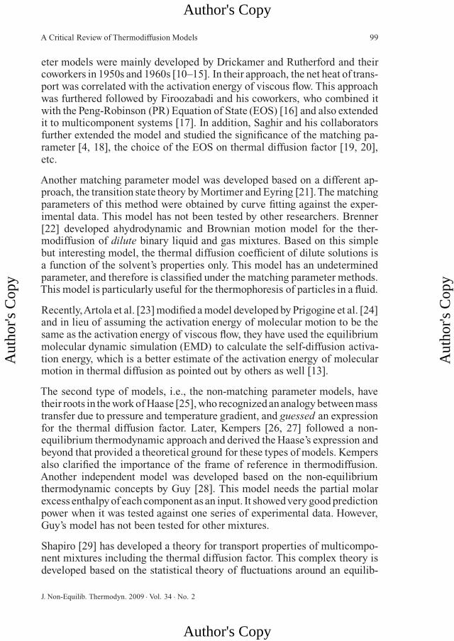
eter models were mainly developed by Drickamer and Rutherford and theircoworkers in 1950s and 1960s [10–15]. In their approach, the net heat of trans-port was correlated with the activation energy of viscous flow. This approachwas furthered followed by Firoozabadi and his coworkers, who combined itwith the Peng-Robinson (PR) Equation of State (EOS) [16] and also extendedit to multicomponent systems [17]. In addition, Saghir and his collaboratorsfurther extended the model and studied the significance of the matching pa-rameter [4, 18], the choice of the EOS on thermal diffusion factor [19, 20],etc.

Another matching parameter model was developed based on a different ap-proach, the transition state theory by Mortimer and Eyring [21].The matchingparameters of this method were obtained by curve fitting against the exper-imental data. This model has not been tested by other researchers. Brenner[22] developed ahydrodynamic and Brownian motion model for the ther-modiffusion of dilute binary liquid and gas mixtures. Based on this simplebut interesting model, the thermal diffusion coefficient of dilute solutions isa function of the solvent’s properties only. This model has an undeterminedparameter, and therefore is classified under the matching parameter methods.This model is particularly useful for the thermophoresis of particles in a fluid.

Recently,Artola et al. [23] modified a model developed by Prigogine et al. [24]and in lieu of assuming the activation energy of molecular motion to be thesame as the activation energy of viscous flow, they have used the equilibriummolecular dynamic simulation (EMD) to calculate the self-diffusion activa-tion energy, which is a better estimate of the activation energy of molecularmotion in thermal diffusion as pointed out by others as well [13].

The second type of models, i.e., the non-matching parameter models, havetheir roots in the work of Haase [25], who recognized an analogy between masstransfer due to pressure and temperature gradient, and guessed an expressionfor the thermal diffusion factor. Later, Kempers [26, 27] followed a non-equilibrium thermodynamic approach and derived the Haase’s expression andbeyond that provided a theoretical ground for these types of models. Kempersalso clarified the importance of the frame of reference in thermodiffusion.Another independent model was developed based on the non-equilibriumthermodynamic concepts by Guy [28]. This model needs the partial molarexcess enthalpy of each component as an input. It showed very good predictionpower when it was tested against one series of experimental data. However,Guy’s model has not been tested for other mixtures.

Shapiro [29] has developed a theory for transport properties of multicompo-nent mixtures including the thermal diffusion factor. This complex theory isdeveloped based on the statistical theory of fluctuations around an equilib-


Author's Copy

Aut

hor's

Cop

y

Author's Copy

Aut

hor's

Cop

y


rium state in a two-vessel system (similar to the two-bulb system in Kempers’theory [26, 27]). However, no direct expression has been derived yet to readilycalculate the thermal diffusion factor or coefficient.

Despite the availability of several thermodiffusion theories, models’ predic-tions may be very different from one another and from the experimentaldata. In some cases even the sign of the thermal diffusion factor cannot bepredicted correctly. Most of the thermodiffusion models rely on the non-equilibrium thermodynamic concepts and provide similar expressions for thecalculations of the thermal diffusion factor. However, due to the complexityof the process and the sensitivity of the models to the equilibrium prop-erties of the mixture or pure components, and the lack of an accurate anduniversally accepted equation of state (EOS), there is no general agreementon the accuracy and validity of various models combined with an EOS. Forinstance, Shukla and Firoozabadi [16] compared the experimental data ofbinary mixtures with the prediction of their model, Kempers’ model [26],and Rutherford’s model [15] all combined with the PR-EOS [30]. They con-cluded that their model [16] was best in predicting the thermal diffusionfactor of hydrocarbon and other systems at nonideal conditions, but awayfrom the critical region. Also, they found that the Rutherford model [15]was better than Kempers’ model [26] in estimating the thermodiffusion co-efficients for hydrocarbon mixtures. On the other hand, Kempers [27] hascriticized the models that need a matching parameter such as [10–16], astheir predicting ability is influenced by the choice of the matching parame-ter. Gonzales-Bagnoli et al. [31] evaluated the performance of some of theabove-mentioned models combined with Soave–Redlich–Kwong (SRK) [32]and PR-EOSs [30]. They concluded that the Haase model [25] generally pro-vides reasonable and stable results; however, Shukla and Firoozabadi [16] andKempers [26, 27] models may be better for some mixtures but produce largeerrors for other mixtures. They also concluded that the Drickamer models[10–13] are erroneous. Some of their conclusions may be debatable, as theShukla and Firoozabadi expression is in fact very similar to, if not the sameas, the Dougherty and Drickamer model [12]. Also, the Haase’s speculativeexpression was later derived by Kempers. In another study, Pan et al. [19] com-pared the latest experimental data for ternary hydrocarbon mixtures againstKempers’ model and the multicomponent model of Firoozabadi et al. [17]combined with PR, volume translated PR (vt-PR), and Perturbed Hard-ChainStatistical Association Fluid Theory (PCSAFT) EOSs [33]. They concludedthat the Firoozabadi et al. model [17] combined with vt-PR or PCSAFT aresuitable for the prediction of the thermodiffusion coefficients for hydrocar-bon and non-hydrocarbon mixtures. Those cases were a few examples thatshow disagreement among researchers regarding the suitability of variousmodels.


Author's Copy

Aut

hor's

Cop

y

Author's Copy

Aut

hor's

Cop

y


Although traditionally the experimental data are less debatable than the theo-retical models, one should note that due to the coupling nature of thermodiffu-sion with other effects such as mixing and convection, inaccurate experimentaldata obtained over four decades may also be responsible for some of thesediscrepancies. New techniques for the measurement of the thermodiffusionfactor, such as optical [34] and x-ray [35] techniques, measurements in mi-crogravity [36], and convective methods [37], may provide accurate data formodel validation.

The above introduction to various models of thermodiffusion reveals that al-though this topic has been the focus of research for more than a century andseveral rather rigorous and semi-empirical models have been developed, thereis no common agreement on the adequacy of any of those models. The modelsneeding a matching parameter apparently match with the experimental databetter, at least for a group of experimental data; however, these models arecriticized because there is no standard and universal method to determine thematching parameters. In addition, a connection between various models islacking and in several cases, some models have overlooked the existence ofthe other models. Therefore, the objective of this study is to provide a criticalreview of some of the most accepted thermodiffusion models. This will hope-fully help identify the research directions in the field. The rest of this paperis structured as follows: since most models, particularly the matching param-eter models, somehow have roots in linear non-equilibrium thermodynamics(LNET), a section will be devoted to LNET and the introduction of the heat oftransport. Subsequently, the models requiring a matching parameter will beintroduced, followed by a comprehensive study on how to estimate the match-ing parameters under various conditions. This part is of great importance, asthe literature is inundated with inconsistent and misleading information aboutthe calculation of matching parameters. The sensitivity of these models withrespect to the magnitude of the matching parameter will be studied as well. InSection 3 the independent models are discussed. Conclusions will be givenin Section 4.

2. Linear non-equilibrium thermodynamics

Thermodiffusion phenomenon as an irreversible process has to be dealt withinnon-equilibrium thermodynamics, also called the “thermodynamics of irre-versible processes”. It is related to the classic equilibrium thermodynamicthrough the assumption that even in an irreversible process, small elemen-tary volumes of the system are in local equilibrium [38]. This assumptionmakes it possible to use the equilibrium thermodynamic relations, such asGibbs and Gibbs–Duhem relations and the Gouy–Stodola theorem in entropy


Author's Copy

Aut

hor's

Cop

y

Author's Copy

Aut

hor's

Cop

y


generation. According to the Gouy–Stodola theorem, entropy generation isproportional to the loss of the available energy. The volumetric rate of entropygeneration σ , which is entropy generation (Sgen) per unit time and per unitvolume multiplied by the absolute temperature (T ), is called the dissipationfunction (ψ):

ψ = Tσ = Td2Sgen

dtdv. (1)

ψ is the rate of energy dissipation per unit volume (W/m3 ).The volumetric rateof entropy generation and also the dissipation function may be used to definethe conjugate forces and fluxes or flows under consideration, such as thosein the coupled heat and mass transfer. It has been argued that, for systemsthat incorporate several components with different temperatures, definingthe forces and fluxes based on the volumetric rate of entropy generation ispreferred or even essential [39]. For the case of thermodiffusion that dealswith one temperature, however, both functions provide the same results, as canbe deduced from Eq. (1). In linear non-equilibrium thermodynamics (LNET),for transport and rate processes, the heat and mass (molar) fluxes with respectto a motionless reference (Ji) are assumed to be linear functions of forces(Xk ), such as temperatures and chemical potentials:

Ji =n

∑i=1

Lik Xk . (2)

Relationships in the form of Eq. (2) are called phenomenological equations(PE). PEs display the interactions between various transport processes. Thecoefficients Lik are called the phenomenological coefficients (PC) and aredefined as follows:

Lik =(∂Ji

∂Xk

)Xj

=(

Ji

Xk

)Xj=0

(j �= k). (3)

Therefore, the PCs Lik represent the flow or flux of transport process i per unitforce of the transport process k when Xj = 0, i.e., at equilibrium. Accordingto Onsager’s reciprocal relations, the matrix Lik is symmetric. The forces aresome forms of the concentration and temperature gradients, both of which cancause mass and heat transfer. Before using the PEs for the coupled heat andthe mass transfer phenomena under study (thermodiffusion), the dissipationfunction (ψ) has to be expressed in terms of the conjugate forces and fluxesof heat and mass transfer:

ψ =n

∑i=1

JiXi. (4)


Author's Copy

Aut

hor's

Cop

y

Author's Copy

Aut

hor's

Cop

y


Then the fluxes may be expressed using the PEs, i.e., Eq. (2). Thermody-namic forces must be chosen such that in the equilibrium state, when theforces vanish, the entropy generation and the dissipation function vanish aswell. Following the non-equilibrium thermodynamics approach, e.g., [38–41], and skipping the derivation, the dissipation function may be written inthe following form, where the thermodynamic forces are independent:

ψ = Tσ = −(

�Jq −n

∑k=1

H k�jk)

· �∇ ln T −n

∑k=1

�jk ·( �∇μk − �F

), (5)

where Jq (J/m2s) is the total rate of heat flux or heat flow, jk (mol/m2s) isthe diffusion molar flow relative to the mean molar velocity (Ji is the molarflux with respect to a motionless reference whereas ji is the diffusive molarflux); H k is the partial molar enthalpy (J/mol), and μk (J/mol) is the chemicalpotential, all for component k . F represents the external force (gravity) actingon the system. The term ∑n

k=1 H k jk is the rate of heat transfer due to massdiffusion. Therefore, the first bracket on the right-hand side of Eq. (5) is therate of heat transfer (heat flow) due to heat conduction only (J ′

q). Equation (5)expresses the energy dissipation per unit volume as the sum of two distinctivecontributions and as the product of the flows and the forces. To simplifyEq. (5), a quantity called the net heat of transport is defined as follows [38]:

Q∗i =

n−1

∑j=1

LqjL−1ij . (6)

It can be shown that for an isothermal system where ∇ ln T = 0, the followingrelationship holds between the heat transfer due to conduction, net heat oftransport, and the molar diffusion fluxes:

J ′q =

n

∑i=1

Q∗i ji and Q∗

i =(

J ′q

ji

)T

if T = constant. (7)

Equation (7) shows that the net heat of transport of component i, Q∗i (J/mol), is

the heat flow per mole of the diffusing component i, required to be absorbedby the region to keep the temperature constant. The net heat of transportin Eq. (7) is based on the diffusion flow ji (mol/m2s) referred to the meanmolar velocity. In a mean molar velocity frame of reference, the sum of all

molar diffusion fluxes is zero, i.e.n∑

i=1ji = 0, and only (n−1) mass fluxes

are independent; therefore, using the definition of the heat of transport, i.e.,Eq. (7), and eliminating the nth component, Eq. (5) can be written in terms of


Author's Copy

Aut

hor's

Cop

y

Author's Copy

Aut

hor's

Cop

y


the (n − 1) independent fluxes:

ψ = Tσ = −n−1

∑k=1

[(Q∗

k − Q∗n

)∇ ln T + ∇T (μk − μn)] · jk . (8)

Note that by writing the dissipation function in this form, the gravity force iseliminated. Now following the concepts of non-equilibrium thermodynamics,from the dissipation function Eq. (8) and using Eq. (2), one can write the molardiffusion flux of component i, as a function of the thermodynamic forces forheat and mass transfer, i.e., ∇ ln T and ∇T (μk):

ji = −n−1

∑k=1

Lik[(

Q∗k − Q∗

n

)∇ ln T + ∇T (μk − μn)]

. (9)

Equation (9) may be used for any multicomponent system. For a binary sys-tem, the conventional diffusive molar flux equation may be written as follows:

j1 = −cD[∇x1 − αx1x2

T∇T], (10)

where c is the molar density (mol/m3), D is the molecular mass diffusioncoefficient (m2/s), and α is the thermal diffusion factor (non-dimensional) bydefinition. At a spatial temperature gradient ∇T , at steady-state mass transfer,the molar flux j1 (and also j2) vanishes. This condition combined with Eqs. (9)and (10) and the Gibbs–Duhem relation at constant pressure and temperature(∑ xidμi = 0) results in the following equation for the thermal diffusion factorfor a binary system:

α = Q∗2 − Q∗

1

x1(∂μ1

/∂x1), (11)

where Q∗1 and Q∗

2 are the net amount of energy that must be provided by thesurrounding and absorbed by the region per mole of components 1 and 2 dif-fusing out, in order to maintain the temperature constant. In a binary mixture,if α (for component 1) obtained from Eq. (11) is positive, component 1 is en-riched at the hot wall [13]. It can be shown that the following Gibbs–Duhemtype of relation holds between the mole fractions and net heats of transportof components 1 and 2:

x1Q∗1 + x2Q∗

2 = 0. (12)

Keeping in mind that x1 and x2 are positive and Q∗1 and Q∗

2 may be either pos-itive or negative, depending on the direction of the heat flow, Eq. (12) impliesthat no heat is absorbed when both components pass in the same direction


Author's Copy

Aut

hor's

Cop

y

Author's Copy

Aut

hor's

Cop

y


through the reference plane in quantities proportional to their mole fractions,i.e., when there is no change in composition. In addition, the net heat of trans-port does not depend on the initial and final states of the diffusing particles,but depends on the mechanism by which diffusion through the reference planeoccurs [9].

Although Eq. (12) was derived a long time ago, satisfactory evaluation of theheat of transport in terms of the measurable properties is still unraveled. Themain features that control thermodiffusion and probably the heat of transportare the size, relative mass, and moment of inertia of the components, as wellas the interaction between the molecules known as the chemical contributions[42, 43]. In some of the models developed and discussed below, particularlythe non-matching parameter or static methods such as Kempers’ model, onlythe mass effects are considered. With the advancement of the computationalcapabilities, “numerical measurement” of the heat of transport and the thermaldiffusion factor has become possible, using the molecular dynamics simula-tion. For instance, Inzoli et al. [44] calculated the heat of transport in thebinary mixture of n-butane in silicate-1. They proved that the heat of trans-port of a component plus the partial molar enthalpy (when the partial molarenthalpy is approximated by the molar energy) in a binary mixture, for a giventemperature, is constant and independent of the local concentration.

3. Matching parameter models

3.1. Description of models

Dougherty and Drickamer model, 1955

Dougherty and Drickamer model [11, 12] is a modification of the modeldeveloped by Rutherford and Drickamer [10] and is based on the conceptof non-equilibrium thermodynamics and incorporates modeling of the netheat of transport. This model has also benefited from the model of Prigogine[24], who is one of the pioneers in non-equilibrium thermodynamics and ismodeling the thermodiffusion process.

Equation (11), which was derived in the previous section, is the starting pointof this model. However, their interpretation and determination of the net heatof transfer was rather speculative. Following the approach of Denbigh [9],Dougherty and Drickamer [10–12] related the net heat of transport to theso-called energy of detaching a molecule from its neighbors WH (J/mole) andthe energy released when a molecule fills a hole WL (J/mole). Taking intoconsideration the different size and shape of the molecules, and assumingthat ψ1 and ψ2 fraction of the molecules move into a hole left by a type 1


Author's Copy

Aut

hor's

Cop

y

Author's Copy

Aut

hor's

Cop

y


and type 2 molecule, respectively, the net heat of transport was expressed asfollows:

Q∗1 = WH1 − ψ1WL, (13)

Q∗2 = WH2 − ψ2WL. (14)

Using some physical justifications, they assumed parametersψ1 andψ2 to beobtained as follows:

ψi = V i

x1V 1 + x2V 2, (15)

where V i is the partial molar volume of component i = 1, 2.

Assuming that the probability of filling a hole already left by a molecule bya molecule type 1 is x1 and by a molecule of type 2 is x2, the energy releasedby a filling process was shown as follows:

WL = x1WH1 + x2WH2. (16)

In an attempt to relate WH to the properties of the solution, such as the excessenergy of mixing per mole (Ue), they assumed that WHi is equal to a fraction(1/τ ) of the difference between the partial molar energy of component i(U i)and the energy of the ideal gas at zero pressure and at the same temperatureas the liquid (U

0ig). Then this difference was related to the properties of the

mixture and the cohesive energy of the component i (ui) as follows:

WHi = − 1

τi(U i − U

0ig) = − 1

τi

(ui + Ue + (n1 + n2)

(∂Ue

∂ni

)), (17)

where Ue is the excess energy of mixing, and n1 and n2 are the number ofmoles of components 1 and 2. They also assumed the cohesive energy to bethe same as the energy of vaporization, here shown as�Evap, i.e., ui = �Evap

(J/mole). In the absence of a suitable EOS, the Hildebrand–Scatchard equation[45, 46] was used to represent the energy of mixing in terms of the propertiesof pure components.

To interpret the physical meaning and estimate the magnitude of τ , Doughertyand Drickamer [11] found some sort of similarity between their interpretationof the energy of detachment of a molecule (WHi) and thermodiffusion as anactivated process with the Andrade–Eyring’s [47, 48] theory and the definitionof the activation energy of viscous flow.Therefore, they assumed the parameterτ in Eq. (17) to be the same as the ratio of the energy of vaporization of liquidto the activation energy of viscous flow defined as parameter n by Eyring and


Author's Copy

Aut

hor's

Cop

y

Author's Copy

Aut

hor's

Cop

y


collaborators [48–50]:

n|Eyring = �Evap

�Evis= τ |Dougherty-Drickamer . (18)

For most materials, it had been observed that the activation energy of viscousflow was 1/3 to 1/4 of the energy of vaporization of the liquid. As a result,Dougherty and Drickamer proposed a constant value of 4 for τ .

In a second publication, Dougherty and Drickamer [12] revised Eq. (11),which has been derived under the mean molar velocity frame of reference( n

∑i=1

�ji = 0)

. They have stated that Eq. (11) implies that the center of mass

of the system is stationary; therefore, to release that hidden assumption, theymodified Eq. (11) to read as follows:

α = M1Q∗2 − M2Q∗

1

M x1(∂μ1

/∂x1), (19)

where Mi is the molecular weight of component i, and M = M1x1 + M2x2. Ina similar approach, they expressed the net heats of transport in terms of WHiand WL, and derived the following equation for α:

α = M2V 1 + M1V 2

M x1(∂μ1

/∂x1) [WH2

V 2− WH1

V 1

]. (20)

Then, similar to their previous work, they related WHi to Eyring’s theory ofviscous flow (to be discussed in the next section). They assumed that one-halfof the activation energy of viscous flow is removed by a molecule, and theother half is dissipated; therefore WHi = (1/2

)�Evis

i .

Equations (19) and (20) are rather ambiguous, in that it is not clear how andunder what frame of reference they have been derived. Note that, if α (ofcomponent 1) obtained from Eqs. (19) and (20) is positive, this component isconcentrated on the hot side.

Tichacek, Kmak, Drickamer model, 1956

Tichacek et al. [13] modified the earlier models of Dougherty and Drickamer[11, 12] in that they wrote the equations in a center-of-volume frame of refer-ence.This model still links the concept of the activation energy of viscous flowto non-equilibrium thermodynamics. However, they modified their interpre-tation of the activation energy of viscous flow. This model is probably the lastversion of Drickamer-type thermodiffusion models. Since in a mean molar


Author's Copy

Aut

hor's

Cop

y

Author's Copy

Aut

hor's

Cop

y


volume frame of reference, ∑ni V iji = 0, Eq. (2) will provide the following

equation:

∑ni V iLik = 0, (21)

where V i is the partial molar volume of component i (m3/mole) and Lik arethe phenomenological coefficients. Following the same approach as that usedto derive Eqs. (11) and (20) will provide an expression for the thermodiffusionfactor in a center-of-volume frame of reference:

α = V 1V 2

V x1(∂μ1

/∂x1) [M2Q∗

2

V 2− M1Q∗

1

V 1

], (22)

where V = x1V 1 + x2V 2 is the molar volume of the solution. In this model,the net heat of transport Q∗

i has been replaced by the new term MiQ∗i (J/g),

which is interpreted as the difference between the total enthalpy transportedby one mole of the moving molecules of type i and the average enthalpy ofone mole of molecules of the same type in the same mixture. They stated thatthe best description of molecular motion of a component in a mixture wouldbe obtained from the measurements of “self-diffusion” of that component inthe mixture (or at least self-diffusion of the pure component) as a function oftemperature and pressure using tagged molecules. Those measurements werenon-existent at that time; therefore, following Eyring’s reaction rate theory,which is based on the hypothesis of the similarity of diffusion and viscousflow, they assumed that MiQ∗

i = (Evis

h

)i. Note that

(Evis

h

)is different from

�Evis, which was used in the previous models [11, 12]. Since a transport ofheat due to moving molecules is concerned here, they concluded that this heatis that part of the activation energy of viscous flow that is transported withthe moving molecules. Recall that in the previous Drickamer model [12], itwas assumed that the heat of detachment of a molecule is one-half of theactivation energy of viscous flow. In their new model, following the work andinterpretation of Bondi [51] on Eyring’s rate theory of flow [48], they realizedthat if they assume the heat of transport during molecular diffusion to beequal to a portion of the activation energy of viscous flow that is responsiblefor local expansion of liquid and forming a hole, their model will be able topredict the thermodiffusion factor for many systems including the associatingmixtures. Using Eyring’s rate theory of viscous flow, this quantity for eachcomponent is obtained as follows:

Evish = R

[(∂ ln (Vη)

∂(1/

T))

P

−(∂ ln (Vη)

∂(1/

T))

V

]= T

(∂P

∂T

)V�V . (23)

Evish (J/mol) is the energy of hole formation, R is the universal gas constant

(J/mol K), V is the liquid molar volume (m3/mol), η is the dynamic viscosity


Author's Copy

Aut

hor's

Cop

y

Author's Copy

Aut

hor's

Cop

y


(Pa.s), P is the pressure (Pa). The first term in the square bracket is the totalactivation energy of viscous flow at constant pressure, and the second term isinterpreted as the energy of motion into the hole. They showed that for manyliquids, including van der Waals liquids, the following equation applies:

Evish

�Evap = �V

V. (24)

In contrast to the previous models, which were recommended for ideal andnon-associating solutions, this model is said to be applicable to nonideal andassociating mixtures as well. This model is also more dynamic compared tothe previous model, e.g., Eq. (17), where a constant matching parameter infact reduces the dynamicity of the model and turns it into a static model.

Shukla and Firoozabadi, 1998

Shukla and Firoozabadi [16] used one of the earlier versions of the Drickamer’smodel [11] and, instead of using the Hildebrand–Scatchard formulas, usedthe volume translated Peng–Robinson (vt-PR) EOS to estimate the partialmolar internal energies and volume of each component in the solution. Theirexpression for calculating the thermodiffusion factor is as follows:

α = U 1/τ1 − U 2

/τ2

x1 (∂μ1/∂x1)T ,P+(V 2 − V 1

) (x1U 1

/τ1 + x2U 2

/τ2)(

x1V 1 + x2V 2)

x1 (∂μ1/∂x1)T ,P. (25)

In derivation of Eq. (25) and for replacement of WHi, Shukla and Firoozabadihave neglected the energy of the ideal gas at zero pressure and at the sametemperature as the liquid (U

0ig), as shown in Eq. (17). Also, further expansion

and simplification of the terms of Eq. (25), and assuming that τ1 = τ2 = τ ,would result in the following equation:

α = V 1V 2

V x1(∂μ1

/∂x1) [ U 1

τV 1− U 2

τV 2

]. (26)

This equation is very similar to Eqs. (20) and (22). Shukla and Firoozabadihave dropped or neglected the term U

0ig in the original equation of Dougherty

and Drickamer, Eq. (17). Also, the sign convention in Eq. (26) is the oppositeto those of Eqs. (20) and (22), i.e., when α (of component 1) is positive, thecomponent 1 migrates to the cold wall.

Although Eq. (25) or (26) was essentially derived in 1955, Shukla and Firooz-abadi’s expression has received more attention, since it was extended to mul-ticomponent mixtures and was successfully linked with the PR-EOS and wasable to predict some experimental data rather well. However, as pointed out


Author's Copy

Aut

hor's

Cop

y

Author's Copy

Aut

hor's

Cop

y


by Tichacek et al. [13], the preliminary model of Dougherty and Drickamer[11] used by Shukla and Firoozabadi is not suitable for nonideal systems. Itwould have been better if the newer version of the model, i.e., Tichacek etal. [13], had been linked with PR-EOS by Shukla and Firoozabadi [16]. Weare currently undertaking a study and the preliminary results show that, atleast for many hydrocarbon mixtures, the Tichacek et al. model linked withthe PR-EOS can predict the thermal diffusion factor better than Kempers,Haase, and Shukla–Firoozabadi models. This is attributed to the dynamicityof the Tichacek et al. model. When the activation energy of viscous flow at apressure and temperature is calculated using the measured viscosity data andused as the net heat of transport, it probably contains some of the features thatinfluence thermodiffusion, such as molecular size, mass, and inertia.

Mortimer and Eyring, 1980

Mortimer and Eyring [21] used the so-called elementary transition state theoryto derive expressions for the Soret and Dufour effects. In the elementary statetheory of isothermodiffusion, the probability per unit time that a molecule oftype i jumps from one equilibrium state to the next is given by

pi = ξkBT

hexp

(−�Gi

RT

), (27)

where ξ is the transmission coefficient, kB is the Boltzmann constant(m2kg/s2K), h is the Planck’s constant (m2kg/s) and�Gi is the free enthalpyof activation (J/mol). The expression for the thermodiffusion factor α is givenas follows:

α = p1�H1 − p2�H2

RT (x2p1 + x1p2), (28)

where p1and p2 are obtained from Eq. (27). Equation (28) has some similaritieswith Eqs. (20) and (22). However, Mortimer and Eyring obtained the activationenthalpies by curve fitting and not using the viscosity data. This implies thatEyring, who was one of the pioneers in the development of the reaction ratetheory, did not consider the activation energy of thermodiffusion the same orrelated to the activation energy of viscous flow.

Kinematical model of Brenner, 2006

Employing a hydrodynamic approach, Brenner [22] has proposed a model tocalculate the thermodiffusion coefficient DT (m2/s K) for binary liquid andgas mixtures. The model, however, is restricted to dilute solutions (i.e., the


Author's Copy

Aut

hor's

Cop

y

Author's Copy

Aut

hor's

Cop

y


mass fraction of one of the components, say solute, is negligible compared tothat of the solvent). The author has used the volume transport theory, whichconsiders a diffusive volume flux accompanying the Fourier heat flux througha single-component fluid. This volume flux is generally nonzero even at thesteady-state condition where the mass flux is essentially zero. Based on thistheory, the thermodiffusion coefficient is a function of the solvent propertiesand is expressed as follows:

DT = λDvβ, (29)

where λ is the nonideality coefficient of O(1), which is not equal to 1 if thesolute is not inert with respect to the solvent; β is the solvent’s coefficient ofthermal expansion; Dv is a non-negative phenomenological coefficient calledthe solvent’s volume diffusivity. In addition, Brenner proposed that the sol-vent’s volume diffusivity is equal to the solvent’s self-diffusion coefficient.Note that the thermodiffusion factor α is related to the thermodiffusion andmass diffusion coefficients DT (m2/sK) and DM (m2/s) and the Soret coeffi-cient ST (K−1) through the following equation:

α = TST = TDT

DM. (30)

The Brenner’s model has been tested against experimental data for varioussolutes (e.g., polystyrene latex particles, sodium dodecyl sulfate, and sodiumpolystyrene sulfonate) in water and it was shown that, as predicted by Eq. (29),the thermodiffusion coefficient for dilute solutions was a function of solventproperties only.

Artola–Rousseau–Galliero Model, 2008

Artola et al. [23] started from Prigogine et al.’s model [24] and modified it forthe effect of molecules of different size and shape. Apparently, the authorshave overlooked Drickamer’s contribution in the theory. Drickamer’s modelconsiders the effect of molecules’ size and shape on thermodiffusion. Artolaet al.’s expression for the thermodiffusion factor is as follows:

α = �G2 −�G1

RT+ M2 − M1

M2 + M1

�G2 +�G1

RT, (31)

where�Gi is the activation free enthalpy of component i = 1, 2, (J/mol). Notethat Eq. (31) is similar to Eqs. (20), (22), and (26), but the term x1

(∂μ1

/∂x1)

has been replaced by RT ; this is valid for ideal solutions only.

As mentioned earlier, Tichacek et al. [13] pointed out that the best descriptionof the molecular motion in a mixture would be described by molecules’ self-


Author's Copy

Aut

hor's

Cop

y

Author's Copy

Aut

hor's

Cop

y


diffusion. However, due to the lack of data for self-diffusion, the activation-free enthalpy has been assumed to be the same as the activation energy ofviscous flow. Artola et al. [23], however, obtained self-diffusion activation-free energy defined through the following equation, using the equilibriummolecular dynamic simulations:

Di = D0i e−�Gi/RT , (32)

where Di and D0i are the self-diffusion coefficients at temperature T and at

a reference temperature T0, respectively. Using the self-diffusion activationenergy instead of the activation energy of viscous flow is definitely one stepforward in thermodiffusion modeling; however, their model would have beenmore efficient if they had incorporated the modifications applied already onthe original Prigogine model by Drickamer and others.

3.2. Activation energy of viscous flow

Despite the gas viscosity, which is very well explained by the kinetic theoryof gases, there is no comprehensive theory capable of predicting the liquidviscosity over a wide range of temperatures and pressures. As a result, manyinvestigators have attempted to use empirical correlations to explain the vis-cosity variation with temperature, free volume, and so on. Below we consideronly those viscosity theories that employ the concept of the activation energyof viscous flow, which is of direct interest to thermodiffusion research.

One of the very first viscosity correlations is that of Arrhenius [52], laterimproved by Andrade [47]:

ln η = A + B

RT, (33)

where A and B are, in general, variables, although have been assumed con-stants in some models. According to Eq. (33), the natural logarithm of theliquid viscosity varies linearly with the reciprocal of the absolute tempera-ture, known as the Arrhenius behavior of viscosity. The parameters A and Bare not universal and vary with material and also with temperature and molarvolume. The Arrhenius behavior is observed for temperatures greater than themelting point and not much higher than the boiling point of the substance.

Later, Eyring and his collaborators found some theoretical ground for theArrhenius equation, where they used the reaction rate theory for the liquidviscosity [48–50]. According to this theory, known as the hole or reaction ratetheory, a liquid is assumed to have a quasi-crystalline structure. Similar toa gas, the liquid is assumed to consist of molecules moving about in empty


Author's Copy

Aut

hor's

Cop

y

Author's Copy

Aut

hor's

Cop

y


spaces or holes. A molecule is pictured as vibrating about an equilibriumposition until the combination of the following two events occurs: (i) Themolecule attains sufficient energy to overcome the attracting forces holding itto its adjacent molecules; (ii) a hole is available into which the molecule canjump. In this theory, the degree of freedom of flow of molecules is assumedto be translational only. The energy required to form a hole of molecular sizein a liquid is equal to the energy of vaporization per molecule. For one moleof liquid, energy of vaporization is expressed as �Evap = H vap– RT, whereH vap is the latent heat of vaporization. The size of the hole could be a fractionof the size of the molecule. The energy required to create such a hole is calledthe activation energy of viscous flow, Evis, and is related to liquid viscosityusing the following equation [48]:

η = Nh

Vexp

(�G

RT

), (34)

where N is the Avogadro’s number and�G is the Gibbs free activation energyof viscous flow (the same quantity as that defined in Eq. [31]). Since �G =�H − T�S, Eq. (34) may be written in the following form:

η =[

Nh

Vexp

(−�S

T

)]exp

(Evis

RT

). (35)

Note that the term �H (J/mol), the activation enthalpy, has been replaced bythe activation energy of viscous flow Evis .This terminology has been borrowedfrom chemistry, where activation energy is the energy that must be overcomein order for a chemical reaction to occur. This may raise some questionsagainst the validity of the Andrade equation at the first place, as in viscousflow no chemical reaction is involved.

The activation energy of viscous flow in Eyring’s theory has to be determinedbefore Eq. (35) can be used to estimate the liquid viscosity. As a secondaryapplication, the net heat of transport in some thermodiffusion models hasbeen approximated by the activation energy of viscous flow. Eyring and hiscoworkers suggested that the magnitude of the activation energy is a fractionof the energy of vaporization [48]. Using Eq. (35), Evis and therefore τ may becalculated for various materials. For a large number of normal liquids, Eyringand his collaborators [48] found that molecules with spherical symmetry haveτ = 3, whereas non-symmetrical molecules have τ greater than 3, usuallyabout 4. For liquid metal, τ is greater and is about 10 to 25, meaning that theactivation energy of viscous flow is a much smaller fraction of the energy ofvaporization.

Doolittle [53] showed that the variation of the natural logarithm of viscos-ity with the reciprocal of temperature deviates from the Arrhenius or linear


Author's Copy

Aut

hor's

Cop

y

Author's Copy

Aut

hor's

Cop

y


behavior over extended temperature ranges. He introduced an empirical equa-tion that correlates the viscosity data with the free space of the liquid for alltemperatures except the freezing point:

ln η = A + B(v0/

vf), (36)

where v0 was defined by Doolittle as the specific volume of the liquid atabsolute zero, and vf as the free volume per mole or gram of the liquid.Later, Cohen and Turnbull [54] theoretically obtained an expression similarto Doolittle’s empirical equation. Macedo and Litovitz [55], in an attempt toaccount for the deficiencies of both the reaction rate and free volume theories,proposed a hybrid equation for viscosity:

η = A exp

(γ v0

vf+ Evis

RT

). (37)

Equation (37) may seem to be useful for calculation of Evis used in the ther-modiffusion models. However, the Macedo and Litovitz model has been crit-icized as being fundamentally incorrect [56, 57].

Another viscosity correlation proposed by Gutmann and Simmons [58] usedtheArrhenius equation (33) with variable activation energy defined as follows:

E = E0

a + b/

T. (38)

In Eq. (38), a and b are constants and E0 is assumed to be an activation energyindependent of temperature.

Eyring et al. [59] recognized that, for example, for compounds n-butanethrough n-nonane, the curve showing the free activation energy against tem-perature has two linear portions with a definite change of slope at about 245 K.Therefore, they concluded that the movement of liquid molecules may not bethrough only translation and jumping of molecules upon acquiring enough ac-tivation energy.As a consequence, they proposed a second theory, which givesa rather different picture of liquid structure and viscous flow. Eyring’s secondtheory, the significant structure theory, considers a liquid to be composed ofsolid-like vibrating molecules and gas-like molecules with translational de-grees of freedom. As a result, their new viscosity equation incorporates twoterms corresponding to the gas and solid viscosities denoted as ηs and ηg ,respectively:

η = Vs

Vηs + V − Vs

Vηg, (39)


Author's Copy

Aut

hor's

Cop

y

Author's Copy

Aut

hor's

Cop

y


where V and Vs are the volumes of the liquid and solid, respectively.Accordingto this theory, a fraction of molecules (Vs/V ) behave like solid molecules andthe rest like gas molecules. Then they showed that Eq. (39) may be writtenin the following form, which incorporates some sort of energy of activation,similar to the hole theory:

η = A exp( ε0

RT

)+ B, (40)

where coefficients A and B are functions of temperatures, volume, and latticeparameters, and ε0 is considered the activation energy for jumping and iswritten as

ε0 = a′EsVs

(V − Vs). (41)

Es is the potential energy of the lattice, and a′ is a kinetic parameter assumedto be 0.0085. The magnitude of ε0 may be obtained graphically from the plotof lnη against 1/T or using Eq. (41) and the method proposed in significantrate theory.

It is obvious that the activation energy of viscous flow defined by this theory isdifferent from that defined by the reaction rate theory. However, the literatureconcerning the viscosity theories based on the concept of energy of activa-tion of viscous flow reveals that despite several deficiencies associated withEyring’s reaction rate theory (Eqs. [34], [35]), it is still the most generallyaccepted equation for calculation of the activation energy of viscous flow. Inthe following section, we will discuss the possible ways of calculating theactivation energies and the matching parameters used in the thermodiffusionmodels.

Activation energy of single component liquids

Equation (35) in Eyring’s theory may be further expanded to express thepre-exponent as a function of parameters such as the molecular weight, tem-perature, and molar volume of the material under consideration [48]. Theexpanded form of Eq. (35) was used by Shukla and Firoozabadi [16] to cal-culate the activation energy of viscous flow. However, since the pre-exponentterm in Eq. (35) is just an approximation, their calculations overestimate thevalues of τ . Nevertheless, as far as the calculation of the activation energyof viscous flow is concerned, the pre-exponent term has no effect if the mea-sured viscosity data are used as input. Evis and τ may be determined fromthe plot of the natural logarithm of the measured viscosity data multiplied bythe molar volume (ln Vη) plotted against 1/RT. When this plot is linear over


Author's Copy

Aut

hor's

Cop

y

Author's Copy

Aut

hor's

Cop

y


a temperature range, the slope of the line is the activation energy of viscousflow over that range. In general, for nonlinear curves, the activation energy attemperature T is the slope of the ln Vη versus 1/RT plot at T :

Evis =(

Rd ln Vη

d(1/T )

)P

. (42)

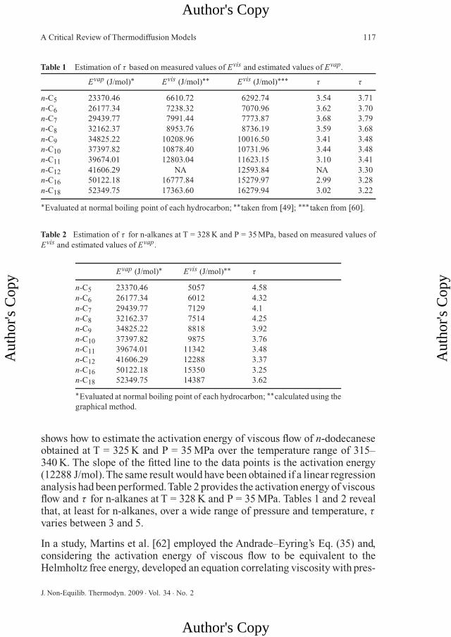
Table 1 lists the values of τ based on the measured values of Evis from [49,60] and the estimated values of �Evap at liquid’s normal boiling point, usingthe NIST database for material’s properties [61]. The data provided in Table 1are based on a linear regression analysis of the measured viscosity data and,therefore, the pre-exponent had no role in the determination of τ .

Note that if a regression analysis is performed on the hybrid Eq. (37), a numberfor the activation energy of viscous flow will be obtained. However, due to thestatistical nature of the regression analysis and the arbitrariness of the valuesof γ and vf ,, we realized that, using Eq. (37), the activation energy cannot beobtained based on a systematic and reliable approach. This is in addition tothe fact that the hybrid Eq. (37) is not theoretically sound.

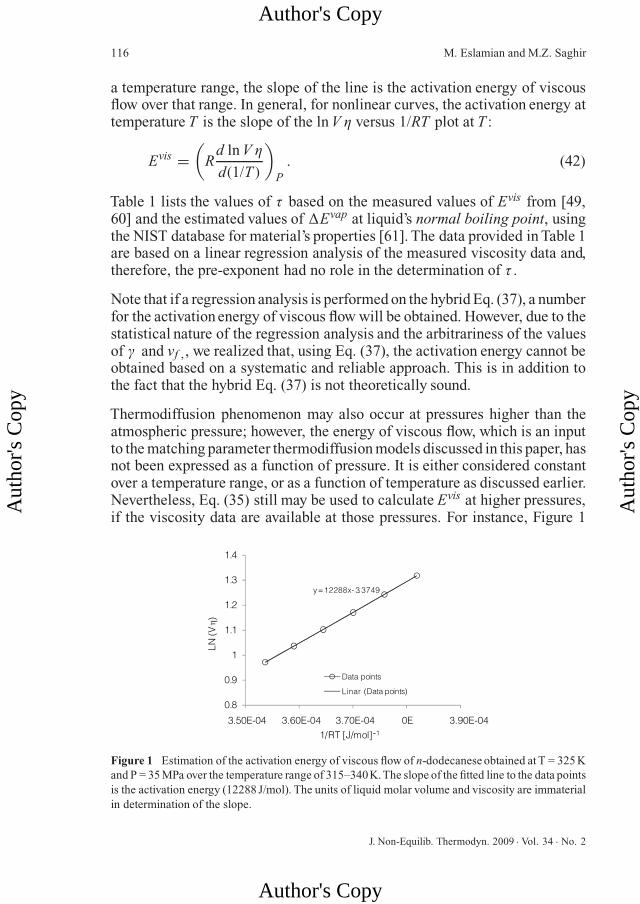
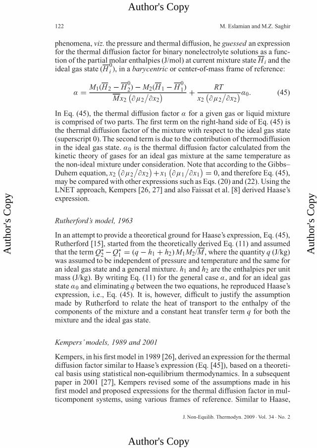
Thermodiffusion phenomenon may also occur at pressures higher than theatmospheric pressure; however, the energy of viscous flow, which is an inputto the matching parameter thermodiffusion models discussed in this paper, hasnot been expressed as a function of pressure. It is either considered constantover a temperature range, or as a function of temperature as discussed earlier.Nevertheless, Eq. (35) still may be used to calculate Evis at higher pressures,if the viscosity data are available at those pressures. For instance, Figure 1

y = 12288x - 3.3749

0.8

0.9

1

1.1

1.2

1.3

1.4

3.50E-04 3.60E-04 3.70E-04 0E 3.90E-04

LN(V

)

1/RT [J/mol]-1

Data points

Linar (Data points)

Figure 1 Estimation of the activation energy of viscous flow of n-dodecanese obtained at T = 325 Kand P = 35 MPa over the temperature range of 315–340K.The slope of the fitted line to the data pointsis the activation energy (12288 J/mol). The units of liquid molar volume and viscosity are immaterialin determination of the slope.


Author's Copy

Aut

hor's

Cop

y

Author's Copy

Aut

hor's

Cop

y


Table 1 Estimation of τ based on measured values of Evis and estimated values of Evap.

Evap (J/mol)∗ Evis (J/mol)∗∗ Evis (J/mol)∗∗∗ τ τ

n-C5 23370.46 6610.72 6292.74 3.54 3.71n-C6 26177.34 7238.32 7070.96 3.62 3.70n-C7 29439.77 7991.44 7773.87 3.68 3.79n-C8 32162.37 8953.76 8736.19 3.59 3.68n-C9 34825.22 10208.96 10016.50 3.41 3.48n-C10 37397.82 10878.40 10731.96 3.44 3.48n-C11 39674.01 12803.04 11623.15 3.10 3.41n-C12 41606.29 NA 12593.84 NA 3.30n-C16 50122.18 16777.84 15279.97 2.99 3.28n-C18 52349.75 17363.60 16279.94 3.02 3.22

∗Evaluated at normal boiling point of each hydrocarbon; ∗∗taken from [49]; ∗∗∗ taken from [60].

Table 2 Estimation of τ for n-alkanes at T = 328 K and P = 35 MPa, based on measured values ofEvis and estimated values of Evap.

Evap (J/mol)∗ Evis (J/mol)∗∗ τ

n-C5 23370.46 5057 4.58n-C6 26177.34 6012 4.32n-C7 29439.77 7129 4.1n-C8 32162.37 7514 4.25n-C9 34825.22 8818 3.92n-C10 37397.82 9875 3.76n-C11 39674.01 11342 3.48n-C12 41606.29 12288 3.37n-C16 50122.18 15350 3.25n-C18 52349.75 14387 3.62

∗Evaluated at normal boiling point of each hydrocarbon; ∗∗calculated using thegraphical method.

shows how to estimate the activation energy of viscous flow of n-dodecaneseobtained at T = 325 K and P = 35 MPa over the temperature range of 315–340 K. The slope of the fitted line to the data points is the activation energy(12288 J/mol).The same result would have been obtained if a linear regressionanalysis had been performed.Table 2 provides the activation energy of viscousflow and τ for n-alkanes at T = 328 K and P = 35 MPa. Tables 1 and 2 revealthat, at least for n-alkanes, over a wide range of pressure and temperature, τvaries between 3 and 5.

In a study, Martins et al. [62] employed the Andrade–Eyring’s Eq. (35) and,considering the activation energy of viscous flow to be equivalent to theHelmholtz free energy, developed an equation correlating viscosity with pres-


Author's Copy

Aut

hor's

Cop

y

Author's Copy

Aut

hor's

Cop

y


sure and temperature. Using various equations of state including the PR-EOS,they provide an expression for calculation of the Helmholtz free energy as afunction of pressure and temperature, considered to be the same as Eyring’sactivation energy of viscous flow. However, comparison of the estimated acti-vation energy of viscous flow obtained using Eyring’s procedure, i.e., plottingln Vη versus 1/RT shows that, for instance, for n-Pentane Eyring’s methodreturns activation energy of 7.3 kJ/mol, whereas the Helmholtz free energyobtained from Martins et al.’s expression is 2.0 kJ/mol. This difference maybe compensated by other parameters when the estimation of viscosity is con-cerned, but when it comes to the application of the activation energy of viscousflow in the thermodiffusion models, it may result in a large difference in thecalculation of the thermodiffusion factor.

Activation energy of mixtures

The most noticeable way of finding the activation energy of viscous flow for amixture is through using a similar method to that of a single-component liquid.At a given temperature, activation energy of the mixture may be obtained asfollows:

Evismix =

(R

d ln (Vη)mix

d(1/T )

)P

. (43)

Singh and Sinha [63, 64] obtained the activation energies of viscous flow forbinary and ternary mixtures at various temperatures and compositions, usingEyring’s rate theory. Their finding suggests that the activation energy of themixture as a function of the activation energy of each component has thefollowing form:

Evismix = x1Evis

1 + x2Evis2 . (44)

For ternary mixtures, however, they found that the plot of the natural logarithmof viscosity versus reciprocal of temperatures may not be linear. As a result,the mixture activation energy of viscous flow may be obtained as the slopeof the curve at a certain temperature. Note that Macedo and Litovitz [55]proposed a different equation for the energy of activation of viscous flow fora binary mixture.

As it can be deduced from the Eyring’s rate theory, the entire mixture behaveslike a single fluid with one viscosity associated with it. Therefore, only onevalue for the activation energy of viscous flow is defined that is associated withthe entire mixture and not each single component. Dougherty and Drickamer[12] proposed that in matching parameter thermodiffusion models, activationenergies of the components in the solution should be used. In practice, how-ever, in most cases the activation energies of pure components have been as-


Author's Copy

Aut

hor's

Cop

y

Author's Copy

Aut

hor's

Cop

y


sumed to be the same as the activation energies of the components in the solu-tion.This discussion reveals the fundamental difference between the activationenergy of viscous flow and the heat of transport in non-equilibrium thermody-namics. While in a multicomponent mixture only one value for the activationenergy of viscous flow is defined, each component has its own heat of transport.

3.3. Sensitivity of matching parameter models with τ

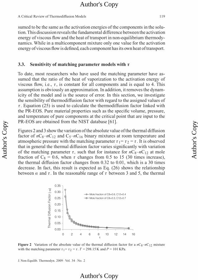
To date, most researchers who have used the matching parameter have as-sumed that the ratio of the heat of vaporization to the activation energy ofviscous flow, i.e., τ , is constant for all components and is equal to 4. Thisassumption is obviously an approximation. In addition, it removes the dynam-icity of the model and is the source of error. In this section, we investigatethe sensibility of thermodiffusion factor with regard to the assigned values ofτ . Equation (25) is used to calculate the thermodiffusion factor linked withthe PR-EOS. Pure material properties such as the specific volume, pressure,and temperature of pure components at the critical point that are input to thePR-EOS are obtained from the NIST database [61].

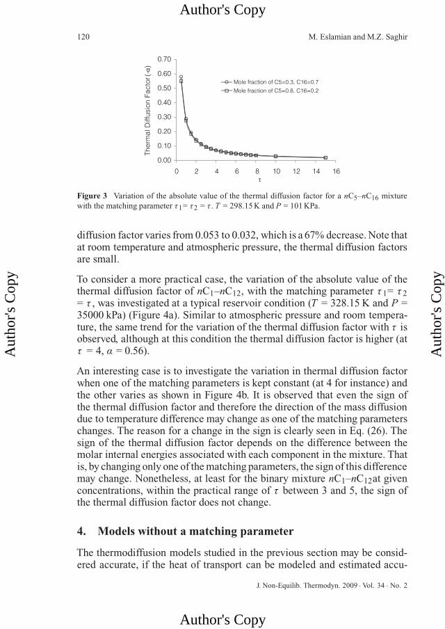
Figures 2 and 3 show the variation of the absolute value of the thermal diffusionfactor of nC8–nC12 and C5–nC16 binary mixtures at room temperature andatmospheric pressure with the matching parameter τ 1= τ 2 = τ . It is observedthat in general the thermal diffusion factor varies significantly with variationof the matching parameter τ , such that for instance for nC8–nC12 at molefraction of C8 = 0.6, when τ changes from 0.5 to 15 (30 times increase),the thermal diffusion factor changes from 0.32 to 0.01, which is a 30 timesdecrease. In fact, this result is expected as Eq. (26) shows the relationshipbetween α and τ . In the reasonable range of τ between 3 and 5, the thermal

0.00

0.05

0.10

0.15

0.20

0.25

0.30

0.35

0 2 4 6 8 10 12 14 16

Ther

mal

Diff

usio

n Fa

ctor

(-)

Mole fraction of C8=0.6, C12=0.4


Figure 2 Variation of the absolute value of the thermal diffusion factor for a nC8–nC12 mixturewith the matching parameter τ1= τ2 = τ . T = 298.15 K and P = 101 KPa.


Author's Copy

Aut

hor's

Cop

y

Author's Copy

Aut

hor's

Cop

y


0.00

0.10

0.20

0.30

0.40

0.50

0.60

0.70

0 2 4 6 8 10 12 14 16

Ther

mal

Diff

usio

n Fa

ctor

(-)



Figure 3 Variation of the absolute value of the thermal diffusion factor for a nC5–nC16 mixturewith the matching parameter τ1= τ2 = τ . T = 298.15 K and P = 101 KPa.

diffusion factor varies from 0.053 to 0.032, which is a 67% decrease. Note thatat room temperature and atmospheric pressure, the thermal diffusion factorsare small.

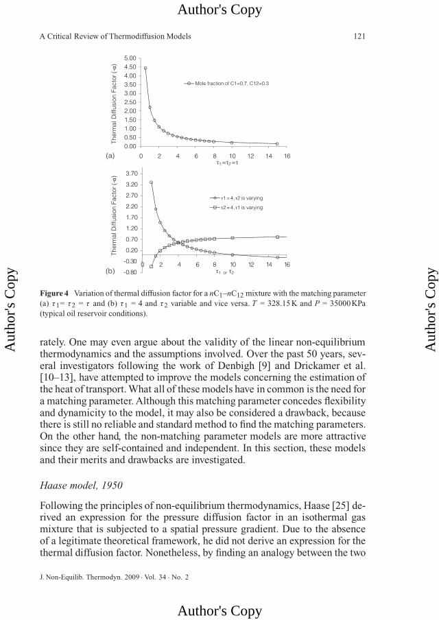
To consider a more practical case, the variation of the absolute value of thethermal diffusion factor of nC1–nC12, with the matching parameter τ 1= τ 2= τ , was investigated at a typical reservoir condition (T = 328.15 K and P =35000 kPa) (Figure 4a). Similar to atmospheric pressure and room tempera-ture, the same trend for the variation of the thermal diffusion factor with τ isobserved, although at this condition the thermal diffusion factor is higher (atτ = 4, α = 0.56).

An interesting case is to investigate the variation in thermal diffusion factorwhen one of the matching parameters is kept constant (at 4 for instance) andthe other varies as shown in Figure 4b. It is observed that even the sign ofthe thermal diffusion factor and therefore the direction of the mass diffusiondue to temperature difference may change as one of the matching parameterschanges. The reason for a change in the sign is clearly seen in Eq. (26). Thesign of the thermal diffusion factor depends on the difference between themolar internal energies associated with each component in the mixture. Thatis, by changing only one of the matching parameters, the sign of this differencemay change. Nonetheless, at least for the binary mixture nC1–nC12at givenconcentrations, within the practical range of τ between 3 and 5, the sign ofthe thermal diffusion factor does not change.

4. Models without a matching parameter

The thermodiffusion models studied in the previous section may be consid-ered accurate, if the heat of transport can be modeled and estimated accu-


Author's Copy

Aut

hor's

Cop

y

Author's Copy

Aut

hor's

Cop

y


0.000.501.001.502.002.503.003.504.004.505.00

0 2 4 6 8 10 12 14 16

Ther

mal

Diff

usio

n Fa

ctor

(-)

1 = 2 =


(a)

-0.80

-0.30

0.20

0.70

1.20

1.70

2.20

2.70

3.20

3.70

0 2 4 6 8 10 12 14 16

Ther

mal

Diff

usio

n Fa

ctor

(-)

1 or 2

1 = 4, 2 is varying

2 = 4, 1 is varying

(b)

Figure 4 Variation of thermal diffusion factor for a nC1–nC12 mixture with the matching parameter(a) τ1= τ2 = τ and (b) τ1 = 4 and τ2 variable and vice versa. T = 328.15 K and P = 35000KPa(typical oil reservoir conditions).

rately. One may even argue about the validity of the linear non-equilibriumthermodynamics and the assumptions involved. Over the past 50 years, sev-eral investigators following the work of Denbigh [9] and Drickamer et al.[10–13], have attempted to improve the models concerning the estimation ofthe heat of transport. What all of these models have in common is the need fora matching parameter. Although this matching parameter concedes flexibilityand dynamicity to the model, it may also be considered a drawback, becausethere is still no reliable and standard method to find the matching parameters.On the other hand, the non-matching parameter models are more attractivesince they are self-contained and independent. In this section, these modelsand their merits and drawbacks are investigated.

Haase model, 1950

Following the principles of non-equilibrium thermodynamics, Haase [25] de-rived an expression for the pressure diffusion factor in an isothermal gasmixture that is subjected to a spatial pressure gradient. Due to the absenceof a legitimate theoretical framework, he did not derive an expression for thethermal diffusion factor. Nonetheless, by finding an analogy between the two


Author's Copy

Aut

hor's

Cop

y

Author's Copy

Aut

hor's

Cop

y


phenomena, viz. the pressure and thermal diffusion, he guessed an expressionfor the thermal diffusion factor for binary nonelectrolyte solutions as a func-tion of the partial molar enthalpies (J/mol) at current mixture state H i and theideal gas state (H

0i ), in a barycentric or center-of-mass frame of reference:

α = M1(H 2 − H02) − M2(H 1 − H

01)

Mx2(∂μ2

/∂x2) + RT

x2(∂μ2

/∂x2)α0. (45)

In Eq. (45), the thermal diffusion factor α for a given gas or liquid mixtureis comprised of two parts. The first term on the right-hand side of Eq. (45) isthe thermal diffusion factor of the mixture with respect to the ideal gas state(superscript 0). The second term is due to the contribution of thermodiffusionin the ideal gas state. α0 is the thermal diffusion factor calculated from thekinetic theory of gases for an ideal gas mixture at the same temperature asthe non-ideal mixture under consideration. Note that according to the Gibbs–Duhem equation, x2

(∂μ2

/∂x2)+x1

(∂μ1

/∂x1) = 0, and therefore Eq. (45),

may be compared with other expressions such as Eqs. (20) and (22). Using theLNET approach, Kempers [26, 27] and also Faissat et al. [8] derived Haase’sexpression.

Rutherford’s model, 1963

In an attempt to provide a theoretical ground for Haase’s expression, Eq. (45),Rutherford [15], started from the theoretically derived Eq. (11) and assumedthat the term Q∗

2 −Q∗1 = (q − h1 + h2) M1M2/M , where the quantity q (J/kg)

was assumed to be independent of pressure and temperature and the same foran ideal gas state and a general mixture. h1 and h2 are the enthalpies per unitmass (J/kg). By writing Eq. (11) for the general case α, and for an ideal gasstate α0 and eliminating q between the two equations, he reproduced Haase’sexpression, i.e., Eq. (45). It is, however, difficult to justify the assumptionmade by Rutherford to relate the heat of transport to the enthalpy of thecomponents of the mixture and a constant heat transfer term q for both themixture and the ideal gas state.

Kempers’ models, 1989 and 2001

Kempers, in his first model in 1989 [26], derived an expression for the thermaldiffusion factor similar to Haase’s expression (Eq. [45]), based on a theoreti-cal basis using statistical non-equilibrium thermodynamics. In a subsequentpaper in 2001 [27], Kempers revised some of the assumptions made in hisfirst model and proposed expressions for the thermal diffusion factor in mul-ticomponent systems, using various frames of reference. Similar to Haase,


Author's Copy

Aut

hor's

Cop

y

Author's Copy

Aut

hor's

Cop

y


Kempers considers the thermal diffusion factor to consist of kinetic and ther-modynamic components. The kinetic component in Kempers’ model, whichcorresponds to an ideal gas state, can be calculated from the kinetic theory ofgases or can be used to calibrate the model against the experimental data. Thethermodynamic component of the thermal diffusion factor is obtained by set-ting up an imaginary experiment in two bulbs containing a mixture connectedby a small tube. The system is small enough to virtually allow eliminationof the convection currents. Assuming that the temperatures in the two bulbsare constant but different, mass will interchange between the bulbs. At steadystate, there will be zero mass flux but a steady heat flux between the two bulbs.To calculate the magnitude of the concentration difference between the twobulbs at steady state, he used this principle that at steady state, the number ofthe microstates with respect to the ideal gas state should be a maximum.

The frame of reference (center of volume, center of mass) plays a rather im-portant role in the final form of the expression for thermal diffusion factorin Kempers’ model. According to Kempers [27], for laboratory experimentswhere the species transport is in one dimension, the system has a constantvolume, and the center of volume is stationary, the equations using the center-of-volume frame of reference can predict the measured data better. In thepresence of small-scale convection, such as underground reservoirs and ex-perimental cells with species transport in more than one dimension due tosuch effects as stirring, Kempers recommends using the equations written inthe center-of-mass frame of reference. Also applicable to the multicomponentsystems, for a binary mixture, Kempers’ expression for the thermal diffusionfactor under center of volume and center of mass are as follows:

Center-of-volume or mean molar volume velocity frame of reference:

α = V 1V 2

V 1x1 + V 2x2

H 2−H02

V 2− H 1−H

01

V 1

x1(∂μ1

/∂x1) + RT

x1(∂μ1

/∂x1)α0. (46)

Center-of-mass or barycentric frame of reference:

α = M1M2

M1x1 + M2x2

H 2−H 02

M2− H1−H 0

1M1

x1(∂μ1

/∂x1) + RT

x1(∂μ1

/∂x1)α0. (47)

α0 is the thermal diffusion factor of the same mixture at the same temperaturein the ideal gas state. It is an input to Kempers’ model, but can be obtainedusing the kinetic theory of gases. Kempers states that his model providesbetter estimations for nonideal mixtures, such as concentrated solutions andnear-critical mixtures. He also observed better prediction when the expression


Author's Copy

Aut

hor's

Cop

y

Author's Copy

Aut

hor's

Cop

y


derived for the center-of-mass frame of reference was used; this is becausein most experimental measurements even in the laboratory, species transportoccurs in multiple dimensions.

To compare the relative contribution of the gas kinetics to that of the non-equilibrium thermodynamics in the final magnitude of the thermal diffusionfactor in liquid mixtures (Eq. [46] and [47]), some computer programmingis required as the gas kinetic theory needs calculation of several complexmathematical functions such as the collision integrals [65, 66]. In general,the ideal gas part of the thermal diffusion factor is small with respect to thethermodynamic part, particularly if the liquid mixture is at high pressure andhigh temperature conditions. However, as showed previously in Figures 2 and3, at room temperature and atmospheric pressure, the thermal diffusion factordue to non-equilibrium thermodynamics may be small and on the same orderof magnitude as that of the ideal gas state. Taylor [67] calculated the thermaldiffusion factor for binary noble gas mixtures at various compositions andtemperatures. Depending on the mixture temperature and composition, α0may vary from 0.01 at low temperatures to 1 at high temperatures. Therefore,it is absolutely important to calculate the thermal diffusion factor in the idealgas state using the gas kinetics. Some models such as the matching parametermethods do not consider this term.

Kempers’ model should be considered to be a good model in the calculationof the thermodiffusion factor, as it provides an expression that is derived fromtheoretical considerations and it is independent of the matching parameters.In addition, it can predict some experimental data rather well. However, thevalidity of his approach and the assumptions made in the derivation of hismodel have not been critically examined by others. In a study, Faissat et al.[8] argued that the theories of Haase [25] and also of Kempers [26, 27] relyon the assumption that the net heats of transport are related solely to thethermostatic values of the mixture, such as enthalpy. This is in contrast to thedynamic models, such as the model of Dougherty and Drickamer [11], whichrelate the net heat of transport to a flow property such as the activation energyof viscous flow as well as the mixture properties. Faissat et al. [8] state thatsince in reality the thermodiffusion phenomenon is a dynamic and activatedprocess, the dynamic models are favored. Farago et al. [68] followed theKempers approach and reconsidered the assumptions and constraints appliedby Kempers. They derived an expression for the thermal diffusion factor as afunction of a property or a field ϕ, which has to be evaluated before a practicalexpression for the calculation of the thermal diffusion factor can be obtained.

α = T

(∂s

∂ϕ

)x1,P

(ϕ2 − ϕ1)

x1(∂μ1

/∂x1), (48)


Author's Copy

Aut

hor's

Cop

y

Author's Copy

Aut

hor's

Cop

y


where s is the molar entropy. Determination of ϕ would require a statisticalor variational approach to evaluate the heat of transport. Farago’s approach isconstructive, as it considers the thermodiffusion phenomenon as a dynamicprocess. In an special case, they showed that if the dynamic parameter ϕ isapproximated by enthalpy, which is a thermostatic property, the Kempers orHaase expressions may be retrieved. Approximating ϕ by a dynamic propertywould definitely improve the prediction ability of the model.

Guy model, 1986

Employing the non-equilibrium thermodynamic concepts and the phe-nomenological equations, Guy [28] has derived an expression for the thermaldiffusion factor in a binary mixture of nonelectrolyte liquids in a barycentricframe of reference in terms of excess enthalpies per unit mass:

α = M2(hxs

2 − hxs1

)x2(∂μ2

/∂x2) , (49)

where the denominator of Eq. (48) is estimated as follows:

x2(∂μ2

/∂x2) = RT

(1 + d ln γ2

d ln x2

). (50)

In Eqs. (49) and (50), M2 is the molecular weight of the lighter component 2,hxs

i = Hxsi

/Mi where h

xsi is the partial excess enthalpy of component i in J/g,

Hxsi is the partial molar enthalpy of component i (J/mol), R is the universal gas

constant, γ2 is an activity coefficient, and x2 is the mole fraction of the lightercomponent 2. Based on the convention he used for α, the heavier component1 is enriched in the cold region.

In derivation of Eq. (48), Guy did not use the net heat of transport definedin non-equilibrium thermodynamics and shown in Eqs. (5)–(7). Instead, herelated the conductive heat flux J ′

q (J/m2s) to the partial excess enthalpies ofcomponents 1 and 2 as follows:

J ′q = Jq − hxs

1 j′1 − hxs2 j′2, (51)

where J ′q and Jq (J/m2s) are defined in Eq. (5), and j′1 and j′2 are the mass

fluxes of components 1 and 2 (g/m2s). Therefore, the key difference betweenthe Guy model and the matching parameter methods is in the replacementof the net heat of transport with the partial excess enthalpy, which can beexperimentally measured or obtained from an equation of state [69].

He used a series of experimental data for the excess enthalpies of ethanol–water mixture and found a very close agreement between calculated and mea-sured α. It appears that this model has not been tested for other mixtures. This


Author's Copy

Aut

hor's

Cop

y

Author's Copy

Aut

hor's

Cop

y


may be readily done, using an EOS, such as PR-EOS to estimate the excessenthalpies for various mixtures [69] and therefore examine the model againstthe experimental data.

5. Conclusions

The merits and shortcomings of the past and present thermodiffusion modelswere studied in an understandable and unambiguous manner. These mod-els were divided into two groups: matching parameter versus non-matchingparameter or self-contained models, the former being dependent on the out-side of thermodynamics, i.e., the reaction rate theory of liquid viscosity. Thesequence of the development of the matching parameter methods and the re-action rate theory was critically reviewed. The ambiguities associated withthese models and the physical meaning and calculation of the activation en-ergy of viscous flow were elucidated. The following specific conclusions maybe drawn:

1. The thermodiffusion process can be considered to be a function of themixture equilibrium properties such as enthalpy and/or the dynamic andnon-equilibrium properties of the fluid or the intermolecular potentials.Theories such as those of Haase and Kempers rely solely on the mixtureequilibrium properties, whereas those of Drickamer and his collaboratorstake into account a sort of dynamic property as well.

2. Drickamer and his collaborators’ models were greatly under the influenceof the reaction rate theory of viscous flow, which had been developedby Eyring and his collaborators just prior to the development of thesethermodiffusion models. The net heat of transport of various componentswas assumed to be related to the activation energy of viscous flow.Althoughit is a good attempt, there is a key difference between the movement ofliquid molecules in a viscous flow and the movement and separation ofdifferent components in thermodiffusion: in the former all molecules movein one direction, whereas in the latter different components may migratein opposite directions. As a result, even assuming the thermodiffusion asan activated process, a close relationship between the activation energy ofthermal diffusion and that of viscous flow seems unrealistic.

3. The entire concepts of the reaction rate theory and the activation energyof viscous flow are debatable. The reaction rate theory of Eyring and hiscollaborators and the way he defines the structure and movement of liquidmolecules by shear forces has been seriously questioned by several inves-tigators, e.g., [70, 71]. In addition, as mentioned before, later, on accountof the shortcomings of the reaction rate theory, Eyring and his coworkers


Author's Copy

Aut

hor's

Cop

y

Author's Copy

Aut

hor's

Cop

y


proposed the significant rate theory to portray the liquid structure and mo-tion and the liquid viscosity in a more realistic manner. It has been pointedout that the viscous flow is not as simple as a chemical reaction that needsa certain amount of thermal energy [70].

4. Having said the above shortcomings of the matching parameter models, itis noteworthy that these models linked with a proper EOS predict the ex-perimental data rather better than the independent models. This is becauseof their dynamic nature.

5. The merit and prediction ability of the matching parameter methods may beimproved by using more sophisticated models for the net heat of transport,such as the self-diffusion activation energy of the components instead ofthe activation energy of viscous flow.

6. Regardless of the reliability of the matching parameter methods, a sen-sitivity analysis showed that, in general, these methods are sensitive tothe choice of the matching parameter used. Using variable matching pa-rameters corresponding to the actual mixture temperature and pressure ishelpful, as using a constant matching parameter turns the dynamic modelinto a static model.

7. The non-matching parameter models of Kempers and Guy seem to bepromising, as they are self-contained. An in-depth non-equilibrium anal-ysis of the thermodiffusion process and refining the assumptions (such asthat performed in [68]) and perhaps incorporating some kinds of dynamicproperties into the model, may help improve the prediction ability of thesemodels.

8. Although a more detailed study would be desirable, our qualitative com-parison revealed that the contribution of gas kinetics in thermodiffusionof a nonideal system should not be ignored, particularly for the mixturesat room temperature and atmospheric pressure that have a rather smallthermal diffusion factor.

9. A discontinuity and lack of understanding and interaction was found amongthe thermodiffusion models. It was observed that some models had over-looked even the existence of other models. This study has provided a rathercomprehensive and critical review of the existing thermodiffusion models,which is a prerequisite to developing new models. It is the most effec-tive way to apply new changes and modifications on the most advancedversions of the existing theories.


Author's Copy

Aut

hor's

Cop

y

Author's Copy

Aut

hor's

Cop

y


AcknowledgmentThis research was partly supported by the Canadian Space Agency (CSA).The first author wishes to thank Ryerson University for the financial support.

References

[1] Ludwig, C., Sitzungsber. Preuss. Akad. Wiss., Phys. Math. Kl., 20 (1856), 539.[2] Soret, C., Arch. Sci. Phys. Nat., 2 (1879), 48.[3] Khawaja, M, Jiang, G., Van-Vaerenbergh, S., Saghir, M.Z., Theoretical analysis and

comparison with experimentation of the molecular and thermal diffusion coefficientsfor a ternary hydrocarbon mixture, J. Non-Equilibr. Thermodyn., 30 (2005), 359.

[4] Yan, Y., Blanco, P., Saghir, M.Z., Bou-Ali, M.M., An improved theoretical model forthermal diffusion coefficient in liquid hydrocarbon mixtures: Comparison betweenexperimental and numerical results, J. Chem. Phys., 129 (2008), 194507.1.

[5] Pan, S., Jiang, G., Yan, Y., Kawaji, M., Saghir, Z., Theoretical prediction of thermaldiffusion in water–methanol, water–ethanol, and water–isopropanol mixtures usingthe PC-SAFT equation of state, J. Non-Equilibr.Thermodyn., 31 (2006), 47–71.

[6] Piazza, R., Thermophoresis: Moving particles with thermal gradients, Soft Matter, 4(2008), 1740.

[7] Duhr, S., Braun, D., Why molecules move along a temperature gradient, Proc. Natl.Acad. Sci. U.S.A., 103 (2006), 19678.

[8] Faissat, B., Knudsen K., Stenby E.H., Montel, F., Fundamental statements aboutthermal diffusion for a multicomponent mixture in a porous medium, Fluid PhaseEquilib., 100 (1994), 209.

[9] Denbigh, K.G., The heat of transport in binary regular solutions, Trans. Faraday Soc.,48 (1952), 1–8.

[10] Rutherford W.M., Drickamer, H.G., Theory of thermal diffusion in liquids and theuse of pressure to investigate the theory, J. Chem. Phys., 22 (1954), 1157–1165.

[11] Dougherty Jr., E.L., Drickamer, H.G., A theory of thermal diffusion in liquids, J.Chem. Phys., 23 (1955), 295–309.

[12] Dougherty Jr., E.L., Drickamer, H.G, Thermal diffusion and molecular motion inliquids, J. Phys. Chem., 59 (1955), 443.

[13] Tichacek, L.J., Kmak, W.S., Drickamer, H.G.,Thermal diffusion in liquids: The effectof non-ideality and association, J. Phys. Chem., 60 (1956), 660.

[14] Rutherford, W.M., Roof, J.G., Thermal diffusion in methane-n-butane mixtures in thecritical region, J. Phys. Chem., 63 (1959), 1506–1511.

[15] Rutherford, W.M., Calculation of thermal diffusion factors for the methane-n-butanesystems in the critical and liquid regions, AIChE J., 9 (1963), 841.

[16] Shukla, K., Firoozabadi, A., A new model of thermal diffusion coefficients in binaryhydrocarbon mixtures, Ind. Eng. Chem. Res., 37 (1998), 3331.

[17] Firoozabadi, A., Ghorayeb, K., Shukla, K., Theoretical model of thermal diffusionfactors in multicomponent mixtures, AIChE J., 46 (2000), 892.

[18] Pan, S., Saghir, M.Z., Kawaji, M., Jiang, G.,Yan,Y., Theoretical approach to evaluatethermodiffusion in aqueous alkanol solutions, J. Chem. Phys., 126 (2007), 014502.


Author's Copy

Aut

hor's

Cop

y

Author's Copy

Aut

hor's

Cop

y


[19] Pan, S.,Yan,Y., Jaber, T.J., Kawaji, M., Saghir, M.Z., Evaluation of thermal diffusionmodels for ternary hydrocarbon mixtures, J. Non-Equilibr. Thermodyn., 32 (2007),241.

[20] Saghir, M.Z., Jiang, C.G. , Derawi, S.O., Stenby, E.H., Kawaji, M., Theoretical andexperimental comparison of the Soret coefficient for water–methanol and water–ethanol binary mixtures, Eur. Phys. J. E, 15 (2004), 241.

[21] Mortimer, R.G., Eyring, H., Elementary transition state theory of the Soret and Du-four effects, Proc. Natl. Acad. Sci. U.S.A., 77 (1980), 1728–1731.

[22] Brenner, H., Elementary kinematical model of thermal diffusion in liquids and gases,Phys. Rev. E, 74 (2006), 036306.

[23] Artola, P.-A., Rousseau, B., Galliero, G., A new model for thermal diffusion: Kineticapproach, J. Am. Chem. Soc., 130 (2008), 10963.

[24] Prigogine, I., de Brouckere, L., Amand, R., Recherches sur la thermodiffusion enphase liquide, Physica 16 (1950), 577.

[25] Haase, R.,Thermodynamics of Irreversible Processes, p. 369,Addison-Wesley, 1969.[26] Kempers, L.J.T.M., A thermodynamic theory of the Soret effect in a multicomponent

liquid, J. Chem. Phys., 90 (1989), 6541.[27] Kempers, L.J.T.M., A comprehensive thermodynamic theory of the Soret effect in a

multicomponent gas, liquid, or solid, J. Chem. Phys., 115 (2001), 6330.[28] Guy,A.G., Prediction of thermal diffusion in binary mixtures of nonelectrolyte liquids

by the use of nonequilibrium thermodynamics, Int. J. Thermophys., 7 (1986), 563.[29] Shapiro, A.A., Fluctuation theory for transport properties in multicomponent mix-

tures: thermodiffusion and heat conductivity, Physica A, 332 (2004), 151.[30] Peng, D.Y., Robinson, D.B., A new two-constant equation of state, Ind. Eng. Chem.

Fundam., 15 (1976), 59.[31] Gonzalez-Bagnoli, M.G., Shapiro, A.A., Stenby, E.H., Evaluation of the thermody-

namic models for the thermal diffusion factor, Philos. Mag., 83 (2003), 2171.[32] Soave, G., Equilibrium constants from a modified Redkh–Kwong equation of state,

Chem. Eng. Sci., 27 (1972), 1197.[33] Song, Y., Lambert, S.M., Prausnitz, J.M., A perturbed hard-sphere-chain equation of

state for normal fluids and polymers, Ind. Eng. Chem. Res., 33 (1994), 1047.[34] Wiegand, S., Thermal diffusion in liquid mixtures and polymer solutions, J. Phys.:

Condens. Matter, 16 (2004), R357.[35] Rondot, S., Aaboubi, O., Baudart, P., Erre, D., Merienne, E., Patat, J.M., Determina-

tion of Soret coefficient and heat of transport in a binary liquid mixture using X-raymicroscopy, Eur. Phys. J. Appl. Phys., 17 (2002), 75.

[36] Yan,Y., Pan, S., Jules, K., Saghir, M.Z., Vibrational effect on thermal diffusion underdifferent microgravity environments, Microgravity Sci. Technol., 19 (2007), 12.

[37] Platten, J.K.,The Soret effect: A review of recent experimental results, J.Appl. Mech.,73 (2006), 5.

[38] Demirel,Y., Sandler, S.I., Linear-nonequilibrium thermodynamics theory for coupledheat and mass transport, Int. J. Heat Mass Transfer, 44 (2001), 2439.

[39] Kjelstrup, S., Bedeaux, D., Non-Equilibrium Thermodynamics of HeterogeneousSystems, p. 56, World Scientific, Singapore, 2008.

[40] De Groot, S.R., Mazur, P., Non-Equilibrium Thermodynamics, Dover, New York,1984.


Author's Copy

Aut

hor's

Cop

y

Author's Copy

Aut

hor's

Cop

y


[41] Demirel, Y., Nonequilibrium Thermodynamics, Elsevier, Amsterdam, 2002.[42] Wiegand, S., Ning, H., Kita, R., Universal concentration dependence of the Soret

coefficient in aqueous systems, J. Non-Equilibr.Thermodyn., 32 (2007), 193–201.[43] Galliero, G., Duguay, B., Caltagirone, J.-P., Montel, F.,Thermal diffusion sensitivity to

the molecular parameters of a binary equimolar mixture, a non-equilibrium moleculardynamics approach, Fluid Phase Equilibria, 208 (2003), 171–188.

[44] Inzoli, I., Simon, J.M., Bedeaux, D., Kjelstrup, S., Thermal diffusion and partialmolar enthalpy variations of n-butane in silicalite-1, J. Phys. Chem. B, 112 (2008),14937–14951.

[45] Scatchard, G., Concentrated solutions of strong electrolytes, Chem. Rev., 8 (1931),321.

[46] Hildebrand, J.H., Scott, R.L., The Solubility of Nonelectrolytes, 3rd ed., Reinhold,New York, 1950.

[47] Andrade, J., Nature (London), 125 (1930), 582.[48] Glasstone, S. Laidler, K.J., Eyring, H., The Theory of Rate Processes. The Kinetics of

Chemical Reactions,Viscosity, Diffusion and Electrochemical Phenomena, McGraw-Hill, New York/London, 1941.

[49] Ewell, R.H., Eyring, H., Theory of viscosity of liquids as a function of temperatureand pressure, J Chem. Phys., 5 (1937), 726–736.

[50] Kauzmann, W., Eyring, H., The viscous flow of large molecules, J. Am. Chem. Soc.,62 (1940), 3113.

[51] Bondi, A., Notes on the rate process theory of flow, J. Chem. Phys., 14 (1946), 591.[52] Arrhenius, S., Meddel Vetenskapsukad. Nohelinst., 3 (1916), 20.[53] Doolittle, A.K., Studies in Newtonian flow. II. The dependence of the viscosity of

liquids on free-space, J. Appl. Phys., 22 (1951), 1471.[54] Cohen, M.H.,Turnbull, D., Molecular transport in liquidsand glasses, J. Chem. Phys.,

31 (1959), 1164.[55] Macedo, P.B., Litovitz,T.A., On the relative roles of free volume and activation energy

in the viscosity of liquids, J. Chem. Phys., 42 (1965), 245.[56] Barlow, A.J., Lamb, J., Matheson, A.J., Viscous behaviour of supercooled liquids,

Proc. R. Soc. Lond. A Math. Phys. Sci., 292 (1966), 322.[57] Hogenboom, D.L., Webb, W., Dixon, J.A., Viscosity of several liquid hydrocarbons

as a function of temperature, pressure, and free volume, J. Chem. Phys., 46 (1967),2586.

[58] Gutmann, F., Simmons, L.M.,The temperature dependence of the viscosity of liquids,J. Appl. Phys., 23 (1952), 977.

[59] Moore, R.J., Gibbs, P., Eyring, H., Structure of the liquid state and viscosity ofhydrocarbons, J. Phys. Chem., 57 (1953), 172.

[60] Kierstead, H.A., Turkevich J., Viscosity and structure of pure hydrocarbons, J. Chem.Phys., 12 (1944), 24.

[61] NIST. Thermodynamic properties of hydrocarbon mixtures database. National Insti-tute of Standards and Technology, version 3.2

[62] Martins, R.J., de MCardoso, M.J.E., Barcia, O.E., A new model for calculating theviscosity of pure liquids at high pressures, Ind. Eng. Chem. Res., 42 (2003), 3824–3830.


Author's Copy

Aut

hor's

Cop

y

Author's Copy

Aut

hor's

Cop

y


[63] Singh, R.P., Sinha, C.P., Viscosities and activation energies of viscous flow of thebinary mixtures of n-hexane with toluene, chlorobenzene, and 1-hexanol, J. Chem.Eng. Data, 29 (1984), 132.

[64] Singh, R.P., Sinha, C.P., Viscosities and activation energies of viscous flow of theternary mixtures of n-hexane, toluene, chlorobenzene, and 1-hexanol, J. Chem. Eng.Data, 30 (1985), 38.

[65] Kincaid, J.M., Cohen, E.G.D., de Haro, M.L.,The Enskog theory for multicomponentmixtures. IV. Thermal diffusion, J. Chem. Phys., 86 (1987), 963.

[66] Hirschfelder, J.O., Curtiss, C.F., Bird, R.B., Molecular Theory of Gases and Liquids,Wiley, New York, 1954.

[67] Taylor, W.L., Thermal diffusion factors for the binary noble gas mixtures, J. Chem.Phys., 72 (1980), 4973.

[68] Farago, J., Rousseau, B., Artola, P.-A., On a variational approach to the Soret coeffi-cient, J. Chem. Phys., 125 (2006), 164508.

[69] Fermeglia, M., Kikic, I., Excess enthalpy calculations by means of equations of state,J. Therm. Anal., 29 (1984), 687.

[70] Mooney, M., A theory of the viscosity of a Maxwellian elastic liquid, J. Rheol., 1(1957), 63.

[71] Brush, S.G., Theories of liquid viscosity, Chem. Rev., 62 (1962), 513.

Paper received: 2009-02-20Paper accepted: 2009-03-31


Author's Copy

Aut

hor's

Cop

y

Author's Copy

Aut

hor's

Cop

y

A Critical Review of Thermodiffusion Models: Role and Significance of the Heat of Transport and the...

Documents

Transcript of A Critical Review of Thermodiffusion Models: Role and Significance of the Heat of Transport and the...