
A Contribution to the Solution of the Inverse Heat Conduction ...
213
A Contribution to the Solution of the Inverse Heat Conduction Problem in Welding Simulation M.Sc. Andreas Pittner BAM-Dissertationsreihe • Band 85 Berlin 2012
-
Upload
khangminh22 -
Category
Documents
-
view
0 -
download
0
Transcript of A Contribution to the Solution of the Inverse Heat Conduction ...
A Contribution to the Solution of the
Inverse Heat Conduction Problem
in Welding Simulation
M.Sc. Andreas Pittner
BAM-Dissertationsreihe • Band 85
Berlin 2012
Impressum
A Contribution to the Solution of theInverse Heat Conduction Problem in Welding Simulation
2012
Herausgeber:
BAM Bundesanstalt für Materialforschung und -prüfung
Unter den Eichen 87
12205 Berlin
Telefon: +49 30 8104-0
Telefax: +49 30 8112029
E-Mail: [email protected]
Internet: www.bam.de
Copyright © 2012 by
BAM Bundesanstalt für Materialforschung und -prüfung
Layout: BAM-Referat Z.8
ISSN 1613-4249
ISBN 978-3-9814634-9-1
Die vorliegende Arbeit entstand an der BAM Bundesanstalt für Materialforschung und -prüfung.
A Contribution to the Solution of the Inverse Heat
Conduction Problem in Welding Simulation
vorgelegt von
Master of Science
Andreas Pittner
aus Stralsund
von der Fakultät V - Verkehrs- und Maschinensysteme
der Technischen Universität Berlin
zur Erlangung des akademischen Grades
Doktor der Ingenieurwissenschaften
Dr.-Ing.
genehmigte Dissertation
Promotionsausschuss:
Vorsitzender: Univ.-Prof. Dr.-Ing. Jörg Krüger
Berichter: Univ.-Prof. Dr.-Ing. Michael Rethmeier
Berichter: Univ.-Prof. Dr.-Ing. habil. Viktor Karkhin
Berichter: Dr.-Ing. Dietmar Weiß
Tag der wissenschaftlichen Aussprache: 01. Juli 2011
Berlin 2012
D 83

v
DANKSAGUNG
Die vorliegende Arbeit entstand während meiner Tätigkeit als wissenschaftlicher Mitarbeiter an der Bundesanstalt für Materialforschung und –prüfung (BAM) in der Fachgruppe 5.5 „Sicherheit gefügter Bauteile“.
An dieser Stelle möchte ich meinem Doktorvater und Fachgruppenleiter Herrn Univ.-Prof. Dr.-Ing. Michael Rethmeier für die Betreuung und Übernahme des Hauptgutachtens dan-ken. Ebenso danke ich Herrn Univ.-Prof. Dr.-Ing. habil. Viktor A. Karkhin von der Polytech-nischen Universität St. Petersburg, Lehrstuhl für Schweiß- und Lasertechnologie, für die Übernahme des Zweitgutachtens sowie intensiven Diskussionen, die maßgeblich zum Gelingen der Arbeit beigetragen haben. Mein Dank gilt des Weiteren Herrn Dr.-Ing. Dietmar Weiß von der Danfoss Power Electronics A/S für die Unterstützung sowie Übernahme des Gutachtens. Außerdem danke ich Herrn Univ.-Prof. Dr.-Ing. Jörg Krüger vom Institut für Werkzeugmaschinen und Fabrikbetrieb (IWF) der Technischen Universität Berlin für die Übernahme des Vorsitzes des Promotionsausschusses. Darüber hinaus möchte ich mei-nem Arbeitsgruppenleiter, Herrn Dr.-Ing. Christopher Schwenk, für die Unterstützung sowie vielen fachlichen Diskussionen während der Anfertigung und Korrektur der Arbeit danken.
Mein weiterer Dank gilt zudem allen Mitarbeiterinnen und Mitarbeitern der Fachgruppe 5.5 „Sicherheit gefügter Bauteile“ für die Unterstützung sowie stets anregenden Diskussionen, welche wesentlich zum Entstehen der Arbeit beigetragen haben. Besonders hervorheben möchte ich hierbei Herrn Thomas Michael, Herrn Stefan Brunow, Herrn Marco Lammers sowie Herrn Sergej Gook, welche mir bei den Versuchsdurchführungen sowie Auswertun-gen hilfreich zur Seite standen. Weiterhin danke ich allen Doktorandinnen und Doktoranden der Fachgruppe 5.5 für die konstruktive und überaus freundschaftliche Zusammenarbeit. Hierbei möchte ich meinen langjährigen Bürokollegen Herrn William Perret erwähnen und ihm für die vielen anregenden Diskussionen danken.
Ein spezieller Dank geht an meine Familie, ohne welche die Anfertigung der Arbeit nicht möglich gewesen wäre. Hierbei möchte ich meine Frau Ute hervorheben, die mich stets liebevoll unterstützt und motiviert hat.
WIDMUNG
Ich widme diese Arbeit meinen Töchtern Helena-Sophie und Hedda-Loreen, die für mich die Quelle meiner Motivation sind.

vii
ABSTRACT
The present thesis provides a contribution to the solution of the inverse heat conduction problem in welding simulation. The solution strategy is governed by the need that the phe-nomenological simulation model utilised for the direct solution has to provide calculation results within short computational time. This is a fundamental criterion in order to apply optimisation algorithms for the detection of optimal model parameter sets.
The direct simulation model focuses on the application of functional-analytical methods for solving the corresponding partial differential equation of heat conduction. In particular, vol-ume heat sources with a bounding of the domain of action are applied. Besides the known normal and exponential distribution, the models are extended by the introduction of parabolically distributed heat sources. Furthermore, the movement on finite specimens under consideration of curved trajectories has been introduced and solved analytically.
The calibration of heat source models against experimental reference data involves the simultaneous adaptation of model parameters. Here, the global parameter space is searched in a randomised manner. However, an optimisation pre-processing is needed to get information about the sensitivity of the weld characteristics like weld pool dimension or objective function due to a change of the model parameters. Because of their low computa-tional cost functional-analytical models are well suited to allow extensive sensitivity studies which is demonstrated in this thesis.
For real welding experiments the applicability of the simulation framework to reconstruct the temperature field is shown. In addition, computational experiments are performed that allow to evaluate which experimental reference data is needed to represent the temperature field uniquely. Moreover, the influence of the reference data like fusion line in the cross section or temperature measurements are examined concerning the response behaviour of the objective function and the uniqueness of the optimisation problem.
The efficient solution of the inverse problem requires two aspects, namely fast solutions of the direct problem but also a reasonable number of degrees of freedom of the optimisation problem. Hence, a method was developed that allows the direct derivation of the energy distribution by means of the fusion line in the cross section, which allows reducing the di-mension of the optimisation problem significantly.
All conclusions regarding the sensitivity studies and optimisation behaviour are also valid for numerical models for which reason the investigations can be treated as generic.

ix
Contents
1 Introduction 1
2 State of the Art 3 2.1 Classification of Welding Simulation ................................................................... 3
2.1.1 Process Simulation ................................................................................. 4 2.1.2 Material Simulation ................................................................................. 5 2.1.3 Structural Simulation .............................................................................. 6
2.2 Welding Temperature Field ................................................................................ 7 2.2.1 Numerical Methods ............................................................................... 12 2.2.2 Analytical Methods ............................................................................... 14
2.3 Solution of Inverse Problems ............................................................................ 20 2.3.1 Optimisation Strategies ........................................................................ 21 2.3.2 Applications for Welding Simulation ..................................................... 25
3 Execution of Experiments 30 3.1 Experimental Investigations.............................................................................. 30 3.2 Computational Investigations ........................................................................... 33
3.2.1 Analytical Heat Conduction Models ...................................................... 33 3.2.1.1 Normal Distribution .............................................................. 36 3.2.1.2 Exponential Distribution ....................................................... 36 3.2.1.3 Parabolic Distribution ........................................................... 36
3.2.2 Extension of Analytical Heat Conduction Models and Evaluation ......... 37 3.2.2.1 Reference Model Setup ....................................................... 37 3.2.2.2 Domain of Action and Energy Distribution ........................... 38 3.2.2.3 Boundary Conditions ........................................................... 40 3.2.2.4 Movement on Curved Trajectories ....................................... 41 3.2.2.5 Comparison with Finite Element Model ............................... 42
3.2.3 Solution of the Inverse Heat Conduction Problem ................................ 43 3.2.3.1 Calculation of Reference Data ............................................. 44 3.2.3.2 Sensitivity of Heat Source Models ....................................... 44
Contents
x BAM-Dissertationsreihe
3.2.3.3 Evaluation of Objective Function ......................................... 45 3.2.3.4 Global Optimisation based on Heuristics ............................. 45 3.2.3.5 Calibration Behaviour of Heat Source Models ..................... 46 3.2.3.6 Application for Welding Experiments ................................... 48
4 Results 50 4.1 Experimental Investigations.............................................................................. 50
4.1.1 Laser-Gas Metal Arc Hybrid Welding ................................................... 50 4.1.2 Laser Beam Welding ............................................................................ 51
4.2 Computational Investigations ........................................................................... 53 4.2.1 Analytical Heat Conduction Models ...................................................... 53
4.2.1.1 Normal Distribution .............................................................. 58 4.2.1.2 Exponential Distribution ....................................................... 62 4.2.1.3 Parabolic Distribution ........................................................... 64
4.2.2 Extension of Analytical Heat Conduction Models and Evaluation ......... 66 4.2.2.1 Energy Distribution and Domain of Action ........................... 66 4.2.2.2 Boundary Conditions ........................................................... 73 4.2.2.3 Movement on Curved Trajectories ....................................... 77 4.2.2.4 Comparison with Finite Element Model ............................... 87
4.2.3 Solution of the Inverse Heat Conduction Problem ................................ 89 4.2.3.1 Calculation of Reference Data ............................................. 89 4.2.3.2 Sensitivity of Heat Source Models ....................................... 94 4.2.3.3 Evaluation of Objective Function ......................................... 97 4.2.3.4 Global Optimisation based on Heuristics ........................... 101 4.2.3.5 Calibration Behaviour of Heat Source Models ................... 104 4.2.3.6 Application for Welding Experiments ................................. 113
5 Discussion of Results 127 5.1 Extension of Analytical Heat Conduction Models and Evaluation ................... 127
5.1.1 Domain of Action and Energy Distribution .......................................... 127 5.1.2 Boundary Conditions .......................................................................... 130 5.1.3 Movement on Curved Trajectories...................................................... 133
Contents
xi
5.1.4 Comparison with Finite Element Model .............................................. 134 5.2 Solution of the Inverse Heat Conduction Problem .......................................... 138
5.2.1 Sensitivity of Heat Source Models ...................................................... 138 5.2.2 Evaluation of Objective Function ........................................................ 141 5.2.3 Calibration Behaviour of Heat Source Models .................................... 144
5.2.3.1 Two Dimensional Parameter Space Studies ..................... 145 5.2.3.2 Three Dimensional Parameter Space Studies ................... 150
5.2.4 Application for Welding Experiments .................................................. 156 5.2.4.1 Laser Beam Welding ......................................................... 156 5.2.4.2 Direct Evaluation of Energy Distribution ............................ 160 5.2.4.3 Laser-Gas Metal Arc Welding ............................................ 164
6 Summary 168
Nomenclature 172
List of Figures 177
List of Tables 182
Literature 183
Own Publications 200

1
1 Introduction
Welding is still one of the most important production techniques in industry. During the last decades the different welding processes that are applied for various materials have been developed mostly on basis of empirical methods. Since the first contributions towards weld-ing simulation by Rykalin [1] and Rosenthal [2, 3] the potential in understanding the funda-mental laws of physics that occur in a welding process has emerged. Nevertheless, the acceptance of welding simulation within the industrial environment and especially among practising welding engineers is still limited. The reason for that development lies in the fact that the real welding process obeys a variety of non linear coupled physical phenomena which are sometimes even not fully physically understood. The capability to create a self consistent model that has the same input parameters as the real process and which is able of predicting the welding temperature field, fluid flow in the weld pool or to make statements regarding the stability of the process is strongly restricted. This is because the simplifica-tions of the physical phenomena yield an input model parameter space that has a not easy to derive relationship with respect to the real process parameter space. In other words this means that for a given set of process parameters the corresponding temperature field can not be predicted by the model directly but only inversely. In particular, the model has to be calibrated against experimental reference data like the fusion line in the cross section or thermal cycle measurements. In this context calibration is denoted for the procedure of performing multiple direct simulations in order to find a model parameter set that provides the optimal agreement between simulated and experimental characteristics of the real weld-ing process, i.e. in terms of the temperature field. The process of model calibration is needed independently on the complexity of the applied simulation model.
The reason for the limited application of welding simulation is quite clear. On the one hand the application of models which take the real process parameters as input and generate detailed statements regarding the physical effects occurring in the process is not a trivial task to solve. On the other hand the current state of the art of having the need to calibrate the welding simulation models against experimental reference data includes two main rea-sons of their restrictive industrial applicability. The first is that only a reproduction of already performed experiments can be done since the reference data has to be known before. The second is that the procedure of finding the optimal configuration of model parameters that produce the best agreement with respect to the reference data is not an easy to solve task. Because the relationship between the model and process parameter space is unknown in general, a multi dimensional optimisation has to be performed. It is comprehensible that if this task is solved manually by a human operator the costs in personnel and time are enor-mous.
The aspects mentioned above are the primary focus of the present Ph.D. thesis. The major goal is to improve the efficiency of the calibration process needed in welding simulation and which is referred to as inverse problem solution. Here, several assumptions have to be made. The first is that only the heat effects of welding in terms of a global temperature field are taken into account since this is the most important part of the simulation chain. The
1 Introduction
2 BAM-Dissertationsreihe
effects occurring during the heat input of the welding source and the phenomena within the weld pool are neglected and only the temperature range below the solidus temperature is of interest. Consequently, the real welding process is simplified to a heat conduction problem. However, with respect to possible subsequent analyses of the residual stress and distortion only the temperature field outside the weld pool is of significance.
The reason for the limited efficiency of inverse problem solution is given by the need for multiple direct simulations runs. It is obvious that in case of numerical models, i.e. finite element models, the computational efforts are high. Therefore, the primary criterion in order to enable an increase in efficiency is to provide fast solutions to the temperature field. One way to fulfil this requirement is to use functional-analytical methods. Since classical ap-proaches obey simplifications in comparison to their numerical counterparts they were ex-tended in such a way that the calculation of a transient three dimensional temperature field due to the action of volume heat sources that are moving on arbitrary curved trajectories under consideration of a finite solid, i.e. flat plate, is possible. In addition, the domain of energy input of the heat source is bounded. Besides the analytical solutions due to a nor-mally and exponentially distributed energy distribution a new parabolic heat source has been introduced. The influence of the linearisation of the heat conduction equation by as-suming temperature independent material data and neglect of phase changes is not con-sidered here. The applicability of the models is evaluated by reconstruction of the tempera-ture field for real welding experiments that serve as reference data.
Furthermore, the application of functional analytical solutions enables to perform sensitivity analyses of volume heat sources with respect to welding temperature field characteristics as weld pool width, length and depth of penetration. This is also the basis for an evaluation of the objective function in dependence on the reference data that is taken into account. It will be investigated to what extent the shape of the objective function is influenced by the reference data to which the model is calibrated against. Moreover, it is demonstrated that the uniqueness of the temperature field characteristics governs the calibration behaviour of the heat source models. All the derived results with respect to the sensitivity of volume heat source models and their calibration behaviour are also valid for numerical discretisation schemes.
The calibration algorithm that will be used here is based on the application of neural net-works. This heuristic approach offers benefit potentials especially if a global optimisation has to be done. In particular, only a few direct simulations are needed to resemble the global behaviour of the objective function. Nevertheless, two criterions are to be considered that govern the calibration behaviour. Besides the computational effort of the direct simula-tions this is the complexity of the optimisation problem, which is given by the number of degrees of freedom. Therefore, the newly developed parabolic heat source will be utilised to derive the energy distribution in thickness direction of a fully penetrated laser beam weld directly from the fusion line in the cross section. This dramatically improves the efficiency of the inverse problem solution by reducing the dimension of the model parameter space by several orders.
3
2 State of the Art
Simulation techniques can contribute in understanding fundamentals related to welding phenomena. Compared to purely experimental methods this may lead to an improvement regarding time and costs especially with respect to the continuous development of new materials and welding processes.
Computational welding mechanics has become a useful tool in order to virtually investigate thermal and mechanical effects of the welding process, which reduces the experimental effort. In this context the precise description of the welding temperature field is one of the most important sub-steps in welding simulation that affects all subsequent analyses [4, 5].
The welding process itself involves various physical effects that are still difficult to describe. Therefore, the modelling is often based on phenomenological models including the funda-mental but simplified physics of the process [6]. An important requirement in computational welding mechanics is the reconstruction of the temperature field as basis for the calculation of phenomena that are governed by the structural transient temperature field, e.g. residual stress and distortion. Methods to solve the temperature field range from functional analytical methods to numerical discretisation schemes. However, the applied simplifications cause the needed calibration of these models with regards to experimental validation data. The aforementioned applied simplifications regarding the phenomena that are relevant for the heat input are the main reason for the still limited predictive character of welding simulation [7].
The next chapters contain an overview of the current state of the art of welding simulation. The main focus is on the simulation of the temperature field as the initial and most important step which influences all subsequent analyses. Furthermore, attention is paid to techniques for the calibration of the thermal models against experiments. The application of heuristic methods will also be considered.
2.1 Classification of Welding Simulation
After Radaj [5] welding simulation can be classified into three main domains. These are:
Process simulation
Material simulation
Structural simulation.
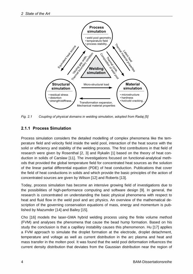
The coupling of these domains by certain input and output quantities is illustrated in Fig. 2.1. As a result of the progress in computer science as well as numerical methods during the last decades, the detailed modelling of physical phenomena is growing continu-ously [8-10]. In the next chapter a short overview of the recent advances in modelling for the three domains stated above is given.
2 State of the Art
4 BAM-Dissertationsreihe
Processsimulation
• weld pool geometry• temperature field• process stability...
Structuralsimulation
• residual stress• distortion• strength/stiffness...
Materialsimulation
• microstructure• hardness• hot/cold cracking...
Micro-structural load
Transformation expansion,Mechanical material properties
Weldingsimulation
Latent heat
Thermal m
aterial properties
Thermal cycle,
Composition of weld pool
Equiv
alent
heat
sour
ceVa
rying
gap w
idth,
Ther
mal bo
unda
ry co
nditio
n
Fig. 2.1 Coupling of physical domains in welding simulation, adopted from Radaj [5]
2.1.1 Process Simulation
Process simulation considers the detailed modelling of complex phenomena like the tem-perature field and velocity field inside the weld pool, interaction of the heat source with the solid or efficiency and stability of the welding process. The first contributions in that field of research were given by Rosenthal [2, 3] and Rykalin [1] based on the theory of heat con-duction in solids of Carslaw [11]. The investigations focused on functional-analytical meth-ods that provided the global temperature field for concentrated heat sources as the solution of the linear partial differential equation (PDE) of heat conduction. Publications that cover the field of heat conductions in solids and which provide the basic principles of the action of concentrated sources are given by Wilson [12] and Roberts [13].
Today, process simulation has become an intensive growing field of investigations due to the possibilities of high-performance computing and software design [9]. In general, the research is concentrated on understanding the basic physical phenomena with respect to heat and fluid flow in the weld pool and arc physics. An overview of the mathematical de-scription of the governing conservation equations of mass, energy and momentum is pub-lished by Mazumder [14] and Bailey [15].
Cho [16] models the laser-GMA hybrid welding process using the finite volume method (FVM) and analyses the phenomena that cause the bead hump formation. Based on his study the conclusion is that a capillary instability causes this phenomenon. Hu [17] applies a FVM approach to simulate the droplet formation at the electrode, droplet detachment, temperature and voltage as well as current distribution in the arc plasma and heat and mass transfer in the molten pool. It was found that the weld pool deformation influences the current density distribution that deviates from the Gaussian distribution near the region of
2.1 Classification of Welding Simulation
5
droplet impact. This is also emphasised by Schnick [18]. Here, the modelling of a TIG arc is considered. It is argued that the formation of the welded joint is mainly given by the stagna-tion pressure of the arc, density of energy input and fluid flow in the molten pool which ex-tends the explanation of bead formation only to be dependent on energy input per unit length. Furthermore, it is discussed that current sophisticated models still need the experi-mental validation due to their limited nature. The simulation of the interaction of metal va-pour in TIG plasma is also published by Yamamoto [19]. The droplet impact on weld pool formation causing a finger like penetration was modelled by Cao [20]. The influence of surface active elements as oxygen, sulphur or selenium on the surface tension and there-fore the flow pattern in the weld pool is investigated numerically by Zhao [21]. The simula-tion of the weld pool deformation by minimisation of the surface energy based on the equi-librium of forces due to arc pressure, surface tension and hydrostatic pressure can be found in Mahrle [22] or Sudnik [23]. The modelling of laser materials processing is presented by Mazumder [24], Lampa [25]. Zhou [26] investigates the governing phenomena in pulsed laser keyhole welding.
Seyffarth [27] gives an overview of the current modelling activities in laser-arc welding processes. Gumenyuk [28] presents the modelling of laser beam welding for light weight construction materials. The simulation of laser beam welding is also considered by Sudnik [23, 29]. A contribution to model laser-arc hybrid welding can be found in Dilthey [30]. There, the weld pool dynamics and their influence on the transport of filler material are investigated. The change of shape of the free surface and the oscillations of the weld pool have not been taken into consideration. The treatment of the welding process as a non-linear dynamic system can be found in Otto [31]. Thus, an excitation of the process with one of its eigenmodes can reduce intrinsic transient fluctuations, e.g. reduce the variation of the depth of penetration during laser surface hardening.
It can be seen that process simulation offers detailed information about the welding proc-ess. However, due to enormous computational requirements and the expert knowledge such models can be mainly found in connection with scientifical investigations. In addition, it has to be stated that still not all physical phenomena are well understood or described mathematically. Especially the couplings of the sub-models are non-linear in nature and are difficult to implement [6]. Moreover, the determination of the material properties, especially in the high temperature range, is challenging.
2.1.2 Material Simulation
Material simulation covers the aspects of microstructural behaviour as hardness and tough-ness, phase transformations and susceptibility with respect to hot or cold cracking phenom-ena. A review of perspective and current work in metallurgical modelling is given in the books of Grong [10] and Janssens [32] or the review paper presented by Babu [33]. Vitek [34] models the microstructural development during weld solidification. In this context the publication of Rappaz [35] has to be mentioned as an extensive overview of modelling approaches and techniques regarding solidification. Zhang [36] discusses an integrated modelling method investigating the effect of the weld thermal cycle on austenite formation and grain growth. The influence of the heat effects of welding, i.e. the thermal cycle, on the microstructure is also considered by Rayamaki [37] and Karkhin [38]. Haidemenopoulos
2 State of the Art
6 BAM-Dissertationsreihe
[39] analyses the evolution of microstructure for high heating and cooling rates in laser welding and hardening under consideration of alloy thermodynamics and kinetics in order to simulate diffusional phase transformations. Holzer [40] models the formation of precipitates for complex martensitic steels. Effects of evolution of precipitates in aluminium alloys are presented by Myhr [41]. Guo [42] solves the linear heat conduction problem including the Stefan problem to account for phase changes. It was found that the solidification speed and temperature gradient at the solidification front governs the microstructure. In this context emphasis was given to the fact that even numerical procedures are difficult to apply for the solution of the moving boundary problem in case of phase changes. Here, one main prob-lem in material modelling within the framework of welding simulation occurs, namely the multi-scale problem. Thiessen [43] applies a dual mesh concept in order to integrate micro-scopic models into macroscopic ones. Ploshikhin [44] simulates the laser beam welding of Al-Mg-Si alloys at different length-scales. In this contribution, the global thermal effects of the welding process (macroscopic) and the simulation of the grain structure at a mesoscopic level according to the inverse solution method after Karkhin [45] are shown. Furthermore, one important aspect is the evaluation of hot and cold cracking susceptibility of the material to be welded. An extensive selection of contributions of material simulation with regards to hot cracking phenomena is published by Böllinghaus [46, 47]
Even though a considerable progress in predicting the microstructural behaviour and micro-scopic effects that take place in welding could be achieved, it is evident that the models incorporate significantly simplified physics. As mentioned, the implementation of micro-scopic models into macroscopic ones is the key issue in order to account for microstructural phenomena. Nevertheless, effective models describing the basic kinetics in phase trans-formations are yet implemented in commercial simulation software. These models are based on the theory of martensitic transformation after Koistinen [48] and the mathematical description of the transformation kinetics during phase changes after Leblond [49, 50].
2.1.3 Structural Simulation
The structural simulation accounts for the thermo-mechanical heat effects of welding as residual stress and distortion, the strength of the weld metal or heat affected zone (HAZ) and evaluation of the stiffness of the structure. Radaj [5] and Goldak [4] summarised many contributions in the field of computational assessment of residual stress and distortion. A review on the evolution of residual stress during welding was done by Wohlfahrt [51, 52] as well as by Nitschke-Pagel [53-55]. Bergheau [56] studied the viscoplastic behaviour of steels during welding and found that the importance of viscoplastic models can be ne-glected in case of the formation of residual stress but may have an effect on the formation of distortion. Doynov [57] applied a chimera meshing technique. Here, the impact of the gap opening during welding on the energy transfer into the work piece is considered. According to the work of Lampa [25] a bidirectional coupling of the temperature and displacement field is done. The temperature field is simulated on a micro-model based on a convection-diffusion model. The results are mapped on a coarser global mesh and the distortions are calculated. Based on the resulting gap opening the temperature field is recalculated. Whereas the influence of the gap opening on the weld pool dimension is of no significance, on the distortion it can yield up to 20% differences in result.
2.2 Welding Temperature Field
7
Mochizuki [58] focuses on the in-process control of distortion during welding of T-fillet joints. The distortion is reduced by an additional cooling torch. Numerical simulations are per-formed to determine the optimal configuration of the water cooling torch.
Pavlyk [59] proposed an integrated simulation framework including the thermal-electrical phenomena between welding wire and work piece (voltage drop), formation of droplets and corresponding transport phenomena and calculated the heat intensity distribution of the heat source and bead formation with SimWeld®. An interface to the multi-purpose finite element code Sysweld® was created in order to perform subsequent analyses of residual stress and distortion. Thus, it is possible to evaluate the influence of different voltage-over-current characteristics of the arc on the resulting displacement field.
In general, there is a significant need of welding simulation with respect to an industrial environment [60]. One reason of the still limited application is the uncertainty of necessary input parameters to the model. Schwenk [61] analysed the influence of the variation of thermo-mechanical material properties on the calculated distortion for different temperature ranges. A sensitivity study concerning the martensite transformation temperature and the effect on the formation of the residual stresses during arc welding can be found in Heinze [62]. Lindgren [63] investigated which input parameters and phenomena are signifi-cant on the simulated residual stresses and distortion. The sensitivity of different hardening models on the simulation of residual stress and distortion was studied by Sakkiettibutra [64]. An important demand is to simplify existing modelling approaches in order to enhance the applicability. A study on the influence of clamping as well as simplified thermo-mechanical models was published by Schenk [65]. Simplified thermo elastic-plastic models for predic-tion of residual stress and distortion of large structures are also presented by Mollicone [66]. The analytical shrinkage force model is applied by Stapelfeld [67]. Ploshikhin [68] presented the software environment Insoft®, which enables the fast calculation of distortion for large scaled structures based on simplified thermo-mechanical models. The suitability of a newly developed welding simulation software simufact.welding® has been studied by Perret [69] for the application in the automotive industry.
2.2 Welding Temperature Field
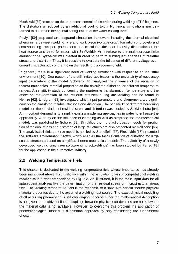
This chapter is dedicated to the welding temperature field whose importance has already been mentioned above. Its significance within the simulation chain of computational welding mechanics is further emphasised by Fig. 2.2. As illustrated, it is the main input data for all subsequent analyses like the determination of the residual stress or microstructural stress field. The welding temperature field is the response of a solid with certain thermo physical material properties due to the action of a welding heat source. The exact physical modelling of all occurring phenomena is still challenging because either the mathematical description is not given, the highly nonlinear couplings between physical sub-domains are not known or the material data is not available. However, to overcome this problem the application of phenomenological models is a common approach by only considering the fundamental effects.
2 State of the Art
8 BAM-Dissertationsreihe
TemperatureField
ResidualStress Field
MicrostructuralState Field
ThermophysicalMaterial Properties
ThermomechanicalMaterial Properties
Hea
t Sou
rce
Fig. 2.2 Overview of computational welding mechanics with weak coupling of thermo mechanical and thermo physical sub-models, adopted from Radaj [5]
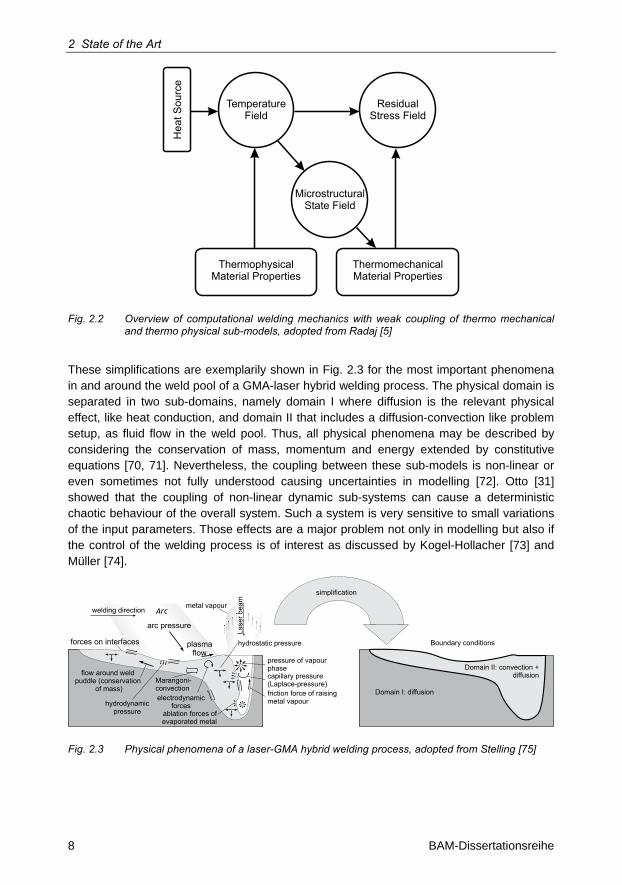
These simplifications are exemplarily shown in Fig. 2.3 for the most important phenomena in and around the weld pool of a GMA-laser hybrid welding process. The physical domain is separated in two sub-domains, namely domain I where diffusion is the relevant physical effect, like heat conduction, and domain II that includes a diffusion-convection like problem setup, as fluid flow in the weld pool. Thus, all physical phenomena may be described by considering the conservation of mass, momentum and energy extended by constitutive equations [70, 71]. Nevertheless, the coupling between these sub-models is non-linear or even sometimes not fully understood causing uncertainties in modelling [72]. Otto [31] showed that the coupling of non-linear dynamic sub-systems can cause a deterministic chaotic behaviour of the overall system. Such a system is very sensitive to small variations of the input parameters. Those effects are a major problem not only in modelling but also if the control of the welding process is of interest as discussed by Kogel-Hollacher [73] and Müller [74].
forces on interfaces
arc pressure
plasmaflow
Arcwelding direction
Lase
r bea
m
friction force of raisingmetal vapour
ablation forces ofevaporated metal
capillary pressure(Laplace-pressure)
pressure of vapourphase
Marangoni-convectionelectrodynamic
forces
flow around weldpuddle (conservation
of mass)
hydrostatic pressure
hydrodynamicpressure
metal vapour
Domain I: diffusion
Domain II: convection +diffusion
Boundary conditions
simplification
Fig. 2.3 Physical phenomena of a laser-GMA hybrid welding process, adopted from Stelling [75]
2.2 Welding Temperature Field
9
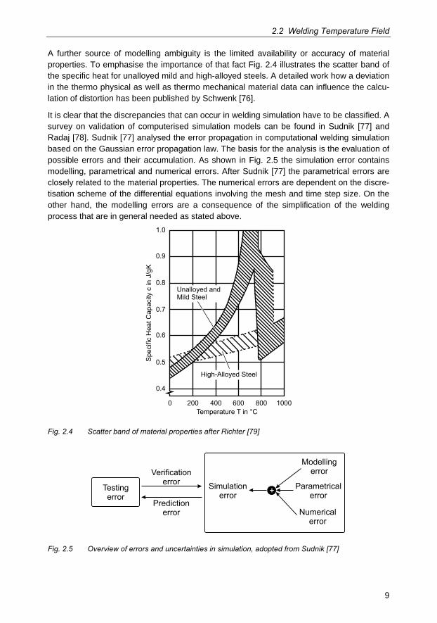
A further source of modelling ambiguity is the limited availability or accuracy of material properties. To emphasise the importance of that fact Fig. 2.4 illustrates the scatter band of the specific heat for unalloyed mild and high-alloyed steels. A detailed work how a deviation in the thermo physical as well as thermo mechanical material data can influence the calcu-lation of distortion has been published by Schwenk [76].
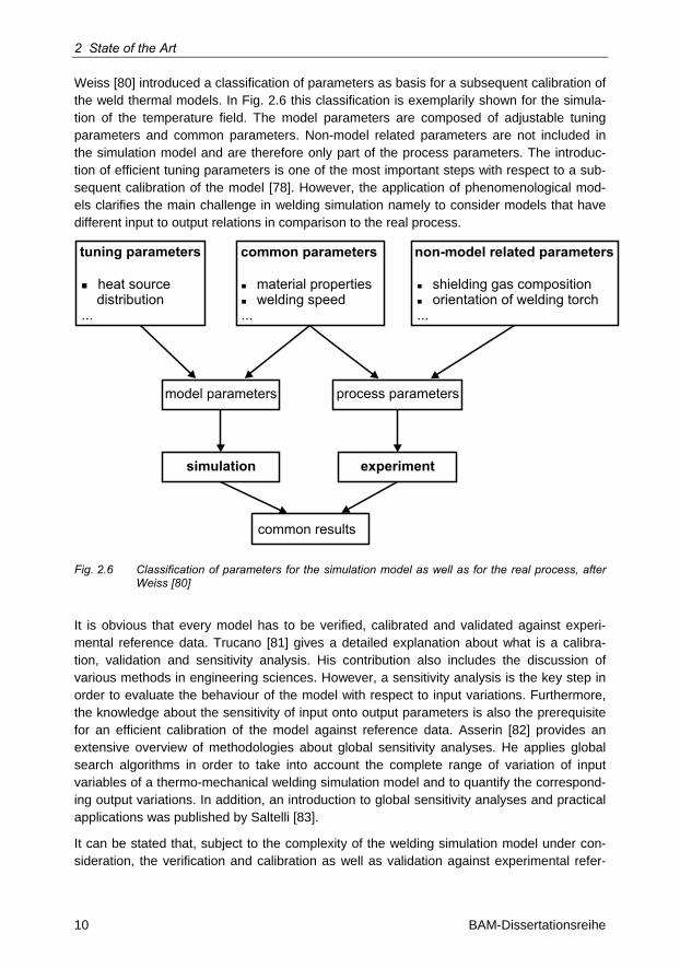
It is clear that the discrepancies that can occur in welding simulation have to be classified. A survey on validation of computerised simulation models can be found in Sudnik [77] and Radaj [78]. Sudnik [77] analysed the error propagation in computational welding simulation based on the Gaussian error propagation law. The basis for the analysis is the evaluation of possible errors and their accumulation. As shown in Fig. 2.5 the simulation error contains modelling, parametrical and numerical errors. After Sudnik [77] the parametrical errors are closely related to the material properties. The numerical errors are dependent on the discre-tisation scheme of the differential equations involving the mesh and time step size. On the other hand, the modelling errors are a consequence of the simplification of the welding process that are in general needed as stated above.
0 200 400 600 800 1000
0.8
0.9
1.0
0.7
0.6
0.4
0.5
Temperature T in °C
Spe
cific
Hea
t Cap
acity
c in
J/g
K
High-Alloyed Steel
Unalloyed andMild Steel
Fig. 2.4 Scatter band of material properties after Richter [79]
Testingerror
Modellingerror
Parametricalerror
Numericalerror
+Simulationerror
Predictionerror
Verificationerror
Fig. 2.5 Overview of errors and uncertainties in simulation, adopted from Sudnik [77]
2 State of the Art
10 BAM-Dissertationsreihe
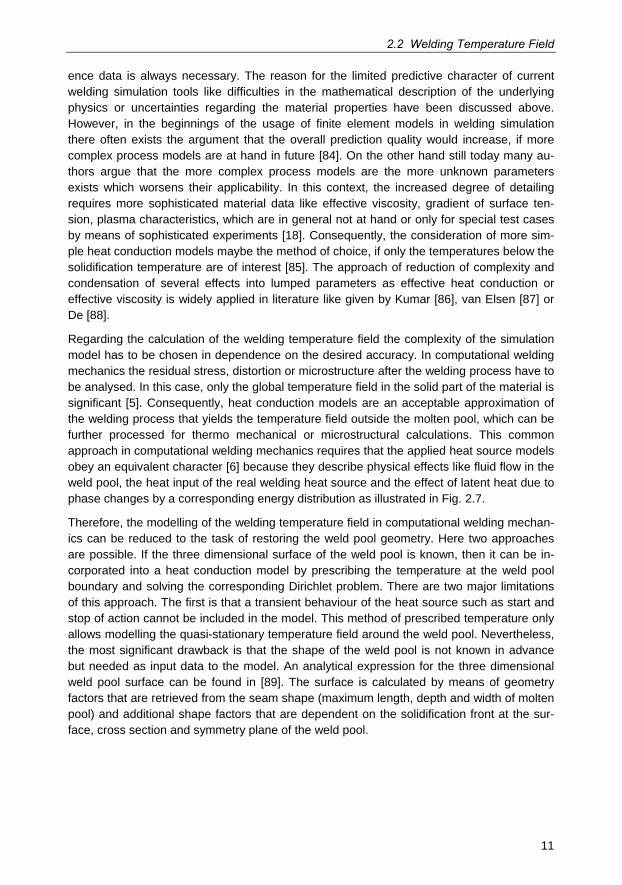
Weiss [80] introduced a classification of parameters as basis for a subsequent calibration of the weld thermal models. In Fig. 2.6 this classification is exemplarily shown for the simula-tion of the temperature field. The model parameters are composed of adjustable tuning parameters and common parameters. Non-model related parameters are not included in the simulation model and are therefore only part of the process parameters. The introduc-tion of efficient tuning parameters is one of the most important steps with respect to a sub-sequent calibration of the model [78]. However, the application of phenomenological mod-els clarifies the main challenge in welding simulation namely to consider models that have different input to output relations in comparison to the real process.
tuning parameters non-model related parameters
model parameters process parameters
simulation experiment
common parameters
common results
� heat sourcedistribution
...
�
�
material propertieswelding speed
...
�
�
shielding gas compositionorientation of welding torch
...
Fig. 2.6 Classification of parameters for the simulation model as well as for the real process, after Weiss [80]
It is obvious that every model has to be verified, calibrated and validated against experi-mental reference data. Trucano [81] gives a detailed explanation about what is a calibra-tion, validation and sensitivity analysis. His contribution also includes the discussion of various methods in engineering sciences. However, a sensitivity analysis is the key step in order to evaluate the behaviour of the model with respect to input variations. Furthermore, the knowledge about the sensitivity of input onto output parameters is also the prerequisite for an efficient calibration of the model against reference data. Asserin [82] provides an extensive overview of methodologies about global sensitivity analyses. He applies global search algorithms in order to take into account the complete range of variation of input variables of a thermo-mechanical welding simulation model and to quantify the correspond-ing output variations. In addition, an introduction to global sensitivity analyses and practical applications was published by Saltelli [83].
It can be stated that, subject to the complexity of the welding simulation model under con-sideration, the verification and calibration as well as validation against experimental refer-
2.2 Welding Temperature Field
11
ence data is always necessary. The reason for the limited predictive character of current welding simulation tools like difficulties in the mathematical description of the underlying physics or uncertainties regarding the material properties have been discussed above. However, in the beginnings of the usage of finite element models in welding simulation there often exists the argument that the overall prediction quality would increase, if more complex process models are at hand in future [84]. On the other hand still today many au-thors argue that the more complex process models are the more unknown parameters exists which worsens their applicability. In this context, the increased degree of detailing requires more sophisticated material data like effective viscosity, gradient of surface ten-sion, plasma characteristics, which are in general not at hand or only for special test cases by means of sophisticated experiments [18]. Consequently, the consideration of more sim-ple heat conduction models maybe the method of choice, if only the temperatures below the solidification temperature are of interest [85]. The approach of reduction of complexity and condensation of several effects into lumped parameters as effective heat conduction or effective viscosity is widely applied in literature like given by Kumar [86], van Elsen [87] or De [88].
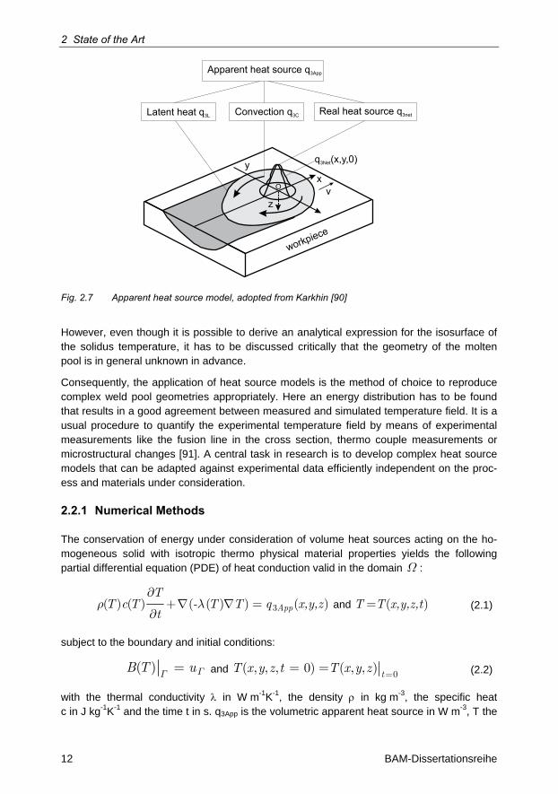
Regarding the calculation of the welding temperature field the complexity of the simulation model has to be chosen in dependence on the desired accuracy. In computational welding mechanics the residual stress, distortion or microstructure after the welding process have to be analysed. In this case, only the global temperature field in the solid part of the material is significant [5]. Consequently, heat conduction models are an acceptable approximation of the welding process that yields the temperature field outside the molten pool, which can be further processed for thermo mechanical or microstructural calculations. This common approach in computational welding mechanics requires that the applied heat source models obey an equivalent character [6] because they describe physical effects like fluid flow in the weld pool, the heat input of the real welding heat source and the effect of latent heat due to phase changes by a corresponding energy distribution as illustrated in Fig. 2.7.
Therefore, the modelling of the welding temperature field in computational welding mechan-ics can be reduced to the task of restoring the weld pool geometry. Here two approaches are possible. If the three dimensional surface of the weld pool is known, then it can be in-corporated into a heat conduction model by prescribing the temperature at the weld pool boundary and solving the corresponding Dirichlet problem. There are two major limitations of this approach. The first is that a transient behaviour of the heat source such as start and stop of action cannot be included in the model. This method of prescribed temperature only allows modelling the quasi-stationary temperature field around the weld pool. Nevertheless, the most significant drawback is that the shape of the weld pool is not known in advance but needed as input data to the model. An analytical expression for the three dimensional weld pool surface can be found in [89]. The surface is calculated by means of geometry factors that are retrieved from the seam shape (maximum length, depth and width of molten pool) and additional shape factors that are dependent on the solidification front at the sur-face, cross section and symmetry plane of the weld pool.
2 State of the Art
12 BAM-Dissertationsreihe
yx
z
O v
q (x,y,0)3Net
workpiece
Latent heat q3L Convection q3C Real heat source q3net
Apparent heat source q3App
Fig. 2.7 Apparent heat source model, adopted from Karkhin [90]
However, even though it is possible to derive an analytical expression for the isosurface of the solidus temperature, it has to be discussed critically that the geometry of the molten pool is in general unknown in advance.
Consequently, the application of heat source models is the method of choice to reproduce complex weld pool geometries appropriately. Here an energy distribution has to be found that results in a good agreement between measured and simulated temperature field. It is a usual procedure to quantify the experimental temperature field by means of experimental measurements like the fusion line in the cross section, thermo couple measurements or microstructural changes [91]. A central task in research is to develop complex heat source models that can be adapted against experimental data efficiently independent on the proc-ess and materials under consideration.
2.2.1 Numerical Methods
The conservation of energy under consideration of volume heat sources acting on the ho-mogeneous solid with isotropic thermo physical material properties yields the following partial differential equation (PDE) of heat conduction valid in the domain W :
App
TT c T - T T q x,y,z
t3( ) ( ) ( ( ) ) = ( )r l
¶+
¶ and T T x,y,z,t= ( ) (2.1)
subject to the boundary and initial conditions:
B T u( ) GG = and tT x y z t T x y z
0( , , , 0) ( , , ) == = (2.2)
with the thermal conductivity in W m-1K-1, the density in kg m-3, the specific heat c in J kg-1K-1 and the time t in s. q3App is the volumetric apparent heat source in W m-3, T the
2.2 Welding Temperature Field
13
temperature in K and x,y,z the spatial coordinates. In general, boundary conditions of first, second or third kind or non-linear boundary conditions as radiative losses can be taken into account as described by the operator B and the corresponding quantity uG [92]. With respect to the initial conditions, an arbitrary temperature distribution can be recognised. It has to be noticed that equation (2.1) is of parabolic type. For a stationary state it becomes elliptic. Because of the temperature dependence of the thermo physical material properties equation (2.1) is nonlinear formulated with respect to the unknown T x y z t( , , , ) .
There are several ways to solve the equation (2.1) numerically. All methods have in com-mon to transfer the problem statement from its strong and continuous formulation in terms of a PDE into a discrete weak formulation, that is given by a set of algebraic equations.
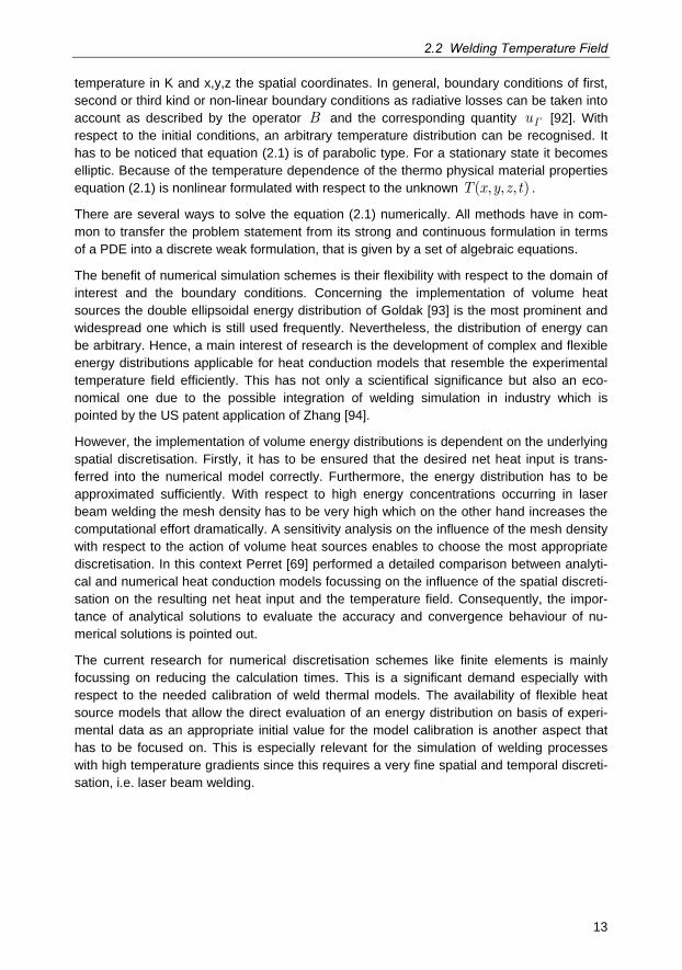
The benefit of numerical simulation schemes is their flexibility with respect to the domain of interest and the boundary conditions. Concerning the implementation of volume heat sources the double ellipsoidal energy distribution of Goldak [93] is the most prominent and widespread one which is still used frequently. Nevertheless, the distribution of energy can be arbitrary. Hence, a main interest of research is the development of complex and flexible energy distributions applicable for heat conduction models that resemble the experimental temperature field efficiently. This has not only a scientifical significance but also an eco-nomical one due to the possible integration of welding simulation in industry which is pointed by the US patent application of Zhang [94].
However, the implementation of volume energy distributions is dependent on the underlying spatial discretisation. Firstly, it has to be ensured that the desired net heat input is trans-ferred into the numerical model correctly. Furthermore, the energy distribution has to be approximated sufficiently. With respect to high energy concentrations occurring in laser beam welding the mesh density has to be very high which on the other hand increases the computational effort dramatically. A sensitivity analysis on the influence of the mesh density with respect to the action of volume heat sources enables to choose the most appropriate discretisation. In this context Perret [69] performed a detailed comparison between analyti-cal and numerical heat conduction models focussing on the influence of the spatial discreti-sation on the resulting net heat input and the temperature field. Consequently, the impor-tance of analytical solutions to evaluate the accuracy and convergence behaviour of nu-merical solutions is pointed out.
The current research for numerical discretisation schemes like finite elements is mainly focussing on reducing the calculation times. This is a significant demand especially with respect to the needed calibration of weld thermal models. The availability of flexible heat source models that allow the direct evaluation of an energy distribution on basis of experi-mental data as an appropriate initial value for the model calibration is another aspect that has to be focused on. This is especially relevant for the simulation of welding processes with high temperature gradients since this requires a very fine spatial and temporal discreti-sation, i.e. laser beam welding.
2 State of the Art
14 BAM-Dissertationsreihe
2.2.2 Analytical Methods
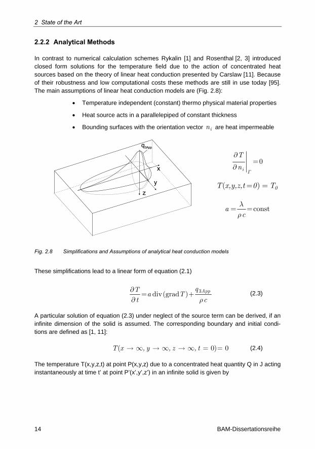
In contrast to numerical calculation schemes Rykalin [1] and Rosenthal [2, 3] introduced closed form solutions for the temperature field due to the action of concentrated heat sources based on the theory of linear heat conduction presented by Carslaw [11]. Because of their robustness and low computational costs these methods are still in use today [95]. The main assumptions of linear heat conduction models are (Fig. 2.8):
Temperature independent (constant) thermo physical material properties
Heat source acts in a parallelepiped of constant thickness
Bounding surfaces with the orientation vector in are heat impermeable
x
y
z
q3Appq3App
i
T
n0
G
¶=
0T x,y,z,t 0 T( = ) =
ac
= =constlr
Fig. 2.8 Simplifications and Assumptions of analytical heat conduction models
These simplifications lead to a linear form of equation (2.1)
AppqT
a Tt c
3= div(grad )+r
¶¶
(2.3)
A particular solution of equation (2.3) under neglect of the source term can be derived, if an infinite dimension of the solid is assumed. The corresponding boundary and initial condi-tions are defined as [1, 11]:
T x , y , z , t( 0) 0 ¥ ¥ ¥ = = (2.4)
The temperature T(x,y,z,t) at point P(x,y,z) due to a concentrated heat quantity Q in J acting instantaneously at time t’ at point P’(x’,y’,z’) in an infinite solid is given by
2.2 Welding Temperature Field
15
x x' y y' z z'
a t t'QT x,y,z,t
c a t t'
2 2 2( ) ( ) ( )
4 ( )
3 2( ) e
4 ( )r p
æ ö- + - + - ÷ç ÷ç- ÷ç ÷ç ÷- ÷çè ø=é ù-ë û
(2.5)
The resulting temperature field T(x,y,z,t) at point P(x,y,z) at time t for a continuous concen-trated heat source of power q in W acting at point P’(x’y’,z’) can the be derived as follows:
t
0
0
qT x,y,z,t G x x',y y',z z',t t' t' T
c( ) ( )d
r= - - - - +ò (2.6)
where T0 is the initial temperature in K. G x x', y y', z z', t t'( )- - - - is referred to as GREEN’S function for PDE’s of parabolic type without source term which can be written as
x x' y y' z z'
a t t'
G x x',y y',z z',t t'a t t'
2 2 2
3 2
( ) ( ) ( )
4 ( )
1( ) *
4 ( )
* e
p
æ ö- + - + - ÷ç ÷ç- ÷ç ÷ç ÷- ÷çè ø
- - - - =é ù-ë û
(2.7)
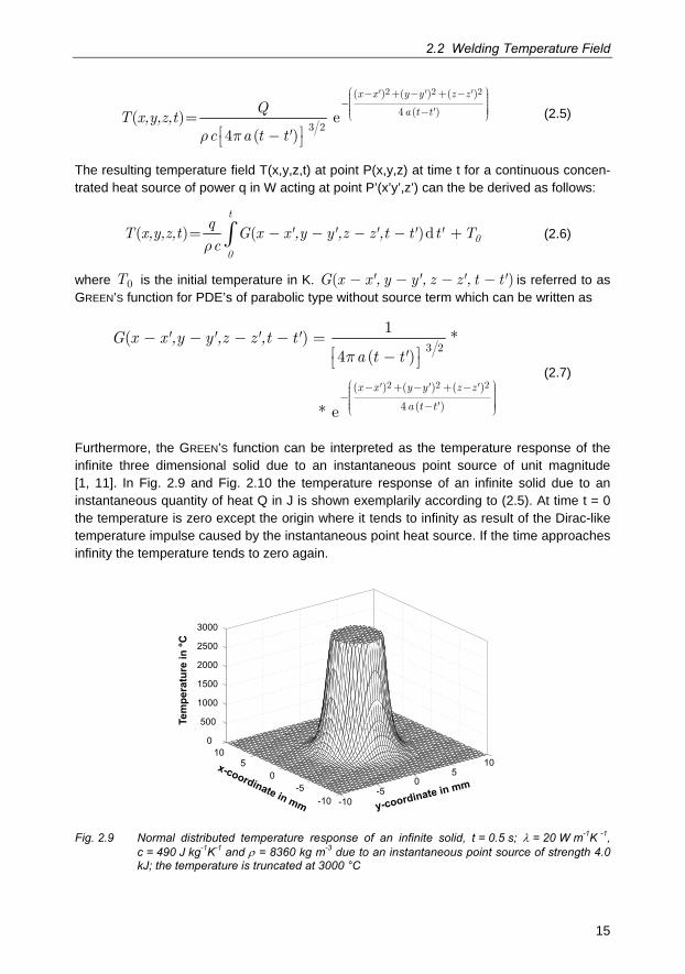
Furthermore, the GREEN’S function can be interpreted as the temperature response of the infinite three dimensional solid due to an instantaneous point source of unit magnitude [1, 11]. In Fig. 2.9 and Fig. 2.10 the temperature response of an infinite solid due to an instantaneous quantity of heat Q in J is shown exemplarily according to (2.5). At time t = 0 the temperature is zero except the origin where it tends to infinity as result of the Dirac-like temperature impulse caused by the instantaneous point heat source. If the time approaches infinity the temperature tends to zero again.
-10-5
05
10
-10-5
05
100
500
1000
1500
2000
2500
3000
Te
mp
era
ture
in
°C
x-coordinate in mm y-coordinate in mm
Fig. 2.9 Normal distributed temperature response of an infinite solid, t = 0.5 s; = 20 W m-1K -1, c = 490 J kg-1K-1 and = 8360 kg m-3 due to an instantaneous point source of strength 4.0 kJ; the temperature is truncated at 3000 °C
2 State of the Art
16 BAM-Dissertationsreihe
-10-5
05
10
-10-5
05
100
500
1000
1500
2000
2500
3000
Te
mp
era
ture
in
°C
x-coordinate in mm y-coordinate in mm
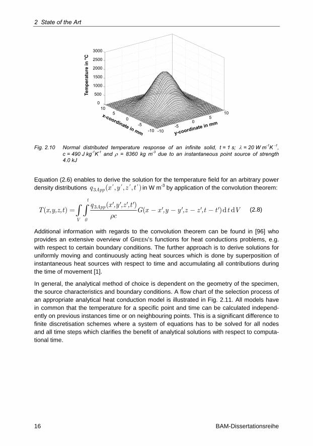
Fig. 2.10 Normal distributed temperature response of an infinite solid, t = 1 s; = 20 W m-1K -1, c = 490 J kg-1K-1 and = 8360 kg m-3 due to an instantaneous point source of strength 4.0 kJ
Equation (2.6) enables to derive the solution for the temperature field for an arbitrary power density distributions Appq x y z t3 ( , , , )¢ ¢ ¢ ¢ in W m-3 by application of the convolution theorem:
t
App
V 0
q x',y',z',t'T x,y,z,t G x x',y y',z z',t t' t V
c3 ( )
( ) ( )d dr
= - - - -ò ò (2.8)
Additional information with regards to the convolution theorem can be found in [96] who provides an extensive overview of GREEN’S functions for heat conductions problems, e.g. with respect to certain boundary conditions. The further approach is to derive solutions for uniformly moving and continuously acting heat sources which is done by superposition of instantaneous heat sources with respect to time and accumulating all contributions during the time of movement [1].
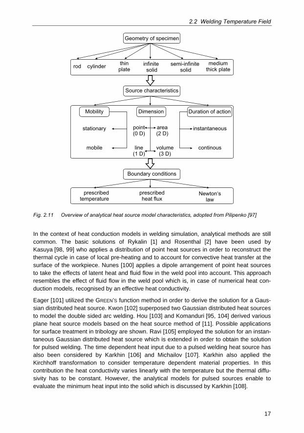
In general, the analytical method of choice is dependent on the geometry of the specimen, the source characteristics and boundary conditions. A flow chart of the selection process of an appropriate analytical heat conduction model is illustrated in Fig. 2.11. All models have in common that the temperature for a specific point and time can be calculated independ-ently on previous instances time or on neighbouring points. This is a significant difference to finite discretisation schemes where a system of equations has to be solved for all nodes and all time steps which clarifies the benefit of analytical solutions with respect to computa-tional time.
2.2 Welding Temperature Field
17
Geometry of specimen
infinitesolid
semi-infinitesolid
mediumthick plate
thinplatecylinderrod
Mobility
stationary
mobile
Dimension
point(0 D)
line(1 D)
area(2 D)
volume(3 D)
Duration of action
instantaneous
continous
Source characteristics
prescribedtemperature
prescribedheat flux
Newton‘slaw
Boundary conditions
Fig. 2.11 Overview of analytical heat source model characteristics, adopted from Pilipenko [97]
In the context of heat conduction models in welding simulation, analytical methods are still common. The basic solutions of Rykalin [1] and Rosenthal [2] have been used by Kasuya [98, 99] who applies a distribution of point heat sources in order to reconstruct the thermal cycle in case of local pre-heating and to account for convective heat transfer at the surface of the workpiece. Nunes [100] applies a dipole arrangement of point heat sources to take the effects of latent heat and fluid flow in the weld pool into account. This approach resembles the effect of fluid flow in the weld pool which is, in case of numerical heat con-duction models, recognised by an effective heat conductivity.
Eager [101] utilized the GREEN’S function method in order to derive the solution for a Gaus-sian distributed heat source. Kwon [102] superposed two Gaussian distributed heat sources to model the double sided arc welding. Hou [103] and Komanduri [95, 104] derived various plane heat source models based on the heat source method of [11]. Possible applications for surface treatment in tribology are shown. Ravi [105] employed the solution for an instan-taneous Gaussian distributed heat source which is extended in order to obtain the solution for pulsed welding. The time dependent heat input due to a pulsed welding heat source has also been considered by Karkhin [106] and Michailov [107]. Karkhin also applied the Kirchhoff transformation to consider temperature dependent material properties. In this contribution the heat conductivity varies linearly with the temperature but the thermal diffu-sivity has to be constant. However, the analytical models for pulsed sources enable to evaluate the minimum heat input into the solid which is discussed by Karkhin [108].
2 State of the Art
18 BAM-Dissertationsreihe
The neglect of the temperature dependence of the thermo physical material properties is one main difference and drawback in comparison to numerical methods. In addition to the Kirchhoff transformation that is also applied by Bertram [109] and which underlies the men-tioned restrictions, Ranatowski [110, 111, 112] proposed a method that considers the non-linear thermo physical material behaviour by an analytical approach. However, this method has to be treated very carefully since the GREEN’S function method can only be applied for linear problems. Karkhin [90] also argues that this approach is invalid in case of a non-linear problem. A discontinuous temperature dependent material property would also yield a discontinuity of the temperature field which violates the law of conservation of energy. In-vestigation regarding the influence of temperature dependence of the material data in weld-ing simulation for an aluminium alloy was presented by Zhu [113].
The implementation of the phenomenon of latent heat based on an analytical approach is extensively described by Karkhin [114, 115]. The effect of the latent heat of melting and solidification on the weld pool geometry in laser beam welding is discussed. Furthermore, the temperature dependence of specific heat is considered by a variable enthalpy. The approach refers to the method of sources and introduction of additional source terms: a heat sink in case of melting and a heat source in case of solidification. This technique is also discussed by van Elsen [87] and compared with different methods in case of a finite difference model.
Due to their advantages with respect to less computation time, analytical heat conduction models are also used for the simulation of multi-pass welding as done by Ramirez [116] and Suzuki [117].
Volumetric heat sources as the double ellipsoidal heat source based on the GREEN’S func-tion method have been published by Nguyen [118, 119]. However, the solution contains a discrepancy with respect to the front part of double ellipsoidal distributed heat source. A correct derivation of the formulae is proposed by Fachinotti [120]. A general method to derive solutions for different heat source distributions like linear, normal or exponential distribution is published by Karkhin [90]. Here a special emphasis was given to the bound-ing of the heat sources with respect to their domain of action. The energy distributions, which were examined, are the normal, exponential and linear distribution. In general, the obtained integrals cannot be solved analytically and have to be processed by means of numerical integration schemes.
The dimension of a plate like geometry can be taken into account by the method of image sources or by expansion of the analytical solution into a FOURIER series which has already been applied by [1-3] to model the temperature field in a medium thick plate under action of concentrated heat sources. This technique yields homogeneous DIRICHLET or NEUMANN boundary conditions at the bounding surfaces. Karkhin [90] extended this method to volu-metric distributed heat sources and showed that the rate of convergence is dependent on the FOURIER number which is a function of heat diffusivity, time of heat diffusion and the square of the plate thickness (characteristic length). The usage of image sources enables the modelling of heat conduction in finite geometries. This fact allows comparing finite ele-ment models with analytical solutions to evaluate the quality of the mesh and the effect of complex boundary conditions. Goldak [93] compares the temperature field in bead on plate welding due to a double ellipsoidal heat source acting on a thick plate with an analytical
2.2 Welding Temperature Field
19
point source solution. However, the double ellipsoidal distribution of the analytical heat source model was not taken into account. In this context, Fachinotti [120] performed a com-parison between the analytical temperature field solution for the double ellipsoidal heat source and the corresponding linear finite element model under the assumption of a semi infinite solid. He could show that both solution methods agree well. Finally, the influence of thermal material non linearities may also effect temperature field that can cause a differ-ence in the cooling times. Here the publication of Kumar [121] has to be noticed. He com-bined analytical and numerical heat conduction models to simulate the temperature field during welding. The numerical model was used to obtain the temperatures in direct vicinity to the heat source in order to account for the non linear material behaviour. The analytical model was employed for the far field temperatures.
More complex boundary conditions like convective heat transfer at the top and bottom sur-face are modelled analytically by Karkhin [90], Ranatowski [112] or Jeong [122]. Neverthe-less, the complexity of the solution increases significantly.
As shown above the analytical heat conduction models are capable of providing the tran-sient temperature field due to volumetrically distributed heat sources acting on finite geome-tries. This is the reason why some authors try to extend these basic solutions in order to simulate the temperature field for more complex problems. A first extension is to consider a movement of the heat source on arbitrary curved trajectories as proposed by Cao [123]. In connection with pipe repair welds an analytical solution of the transient temperature field for a point source is utilised so that the movement on curved trajectories on a semi-infinite solid can be modelled. Recently, Winczek [124] expanded this approach for volume heat sources. The energy distribution under consideration is normal in through thickness direc-tion and symmetrical GAUSSIAN distributed in the plane of movement. Both methods have in common that the direction vector of movement is incorporated in the analytical solution for the temperature field directly on basis of global coordinates. An application for finite geome-tries as well as asymmetrical energy distribution like the double ellipsoidal one is not con-sidered.
The utilisation of analytical temperature field models for complex geometries, i.e. different joint-types, has been an interesting field of research. Jeong [125] applies the conformal mapping technique to obtain an analytical temperature field model for the simulation of fillet arc welding. He applies the SCHWARZ-CHRISTOFFEL transformation [126] to map the solution of the half-plane onto the geometry of the fillet joint. This approach has to be treated with attention because only the Laplace equation is invariant to conformal mapping. In the case of the Poisson equation the source term should be transformed, too. If the analytical heat conduction models equation (2.3) is taken in account, a parabolic/elliptic type of PDE exists. Therefore, conformal mapping can only be applied for special simplified cases as described in 127]. In this framework Guodong [128] publishes the application of conformal mapping to model the temperature field for a heat source that moves at the perimeter of a cylinder. Since in this case the diameter is rather large the conformal mapping is nothing else like a geometrical mapping by unwrapping the cylindrical shape onto a corresponding plate. Tusek [129] applied conformal mapping techniques in order to evaluate the influence of different joint types on the welding efficiency by transforming the Gaussian distributed heat intensity distribution for a flat surface (I-joint) onto different geometries.
2 State of the Art
20 BAM-Dissertationsreihe
In summary, it can be concluded that the development of analytical methods to solve for the temperature field during welding is still a very active field of research. This is because of the advantages with respect to computational costs. The low calculation time promises benefit potentials, especially with respect to the solution of the inverse heat conduction problem. Here, a major task is to develop flexible heat source models and the associated functional analytical expressions for the temperature that enable an efficient calculation of the experi-mental temperature field. As stated above, effects as fluid flow in the weld pool or material non linearities have to be approximated by a corresponding energy distribution which can be a superposition of fundamental distributions. A further prerequisite of heat source mod-els is to obey a domain of action which ensures a physical correct energy input as sug-gested by Karkhin [90].
Regarding the extension of analytical temperature field models for more complex geome-tries, the focus should be on plate like geometries because the application of conformal mapping techniques seems not to be promising. However, with respect to the movement on curved trajectories the extension to finite geometries (plate) under consideration of arbitrary distributed volume heat sources would provide a field of possible applications.
2.3 Solution of Inverse Problems
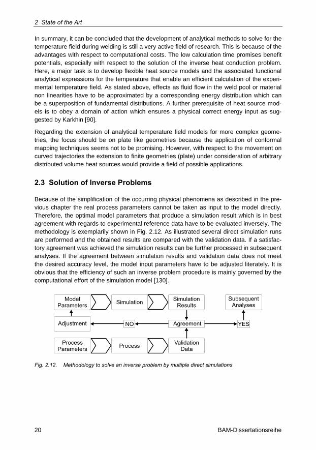
Because of the simplification of the occurring physical phenomena as described in the pre-vious chapter the real process parameters cannot be taken as input to the model directly. Therefore, the optimal model parameters that produce a simulation result which is in best agreement with regards to experimental reference data have to be evaluated inversely. The methodology is exemplarily shown in Fig. 2.12. As illustrated several direct simulation runs are performed and the obtained results are compared with the validation data. If a satisfac-tory agreement was achieved the simulation results can be further processed in subsequent analyses. If the agreement between simulation results and validation data does not meet the desired accuracy level, the model input parameters have to be adjusted literately. It is obvious that the efficiency of such an inverse problem procedure is mainly governed by the computational effort of the simulation model [130].
SimulationModelParameters
SimulationResults
Adjustment
ValidationData
AgreementNO YES
SubsequentAnalyses
ProcessProcessParameters
Fig. 2.12. Methodology to solve an inverse problem by multiple direct simulations
2.3 Solution of Inverse Problems
21
In case of welding simulation, the significant inverse problem that has to be solved is the reconstruction of the temperature field because it governs all subsequent analyses. This is the most demanding and time consuming task to be done [131]. Thus, the application of optimisation algorithms has been established in this context. The next chapter will focus on the classification of optimisation strategies with respect to the solution of the inverse heat conduction problem in welding simulation.
2.3.1 Optimisation Strategies
As previously discussed the solution of the inverse heat conduction problem requires the evaluation of model input parameter sets that yield a simulation result being in optimal agreement with experimental validation data. In equation (2.9) an optimisation problem is defined as a least-squares sum. The objective function can then be formulated as:
N
Experiment,i Simulation,ii
Obj p u u p Minimum2
=1
1( ) ( )
2é ù= - ë ûå (2.9)
where Simulation iu , and Experiment iu , corresponds to the vector of simulated data sets and experimental data sets respectively. The design variables which correspond to the degree of freedom of the optimisation problem are denoted by the vector of parameters p .
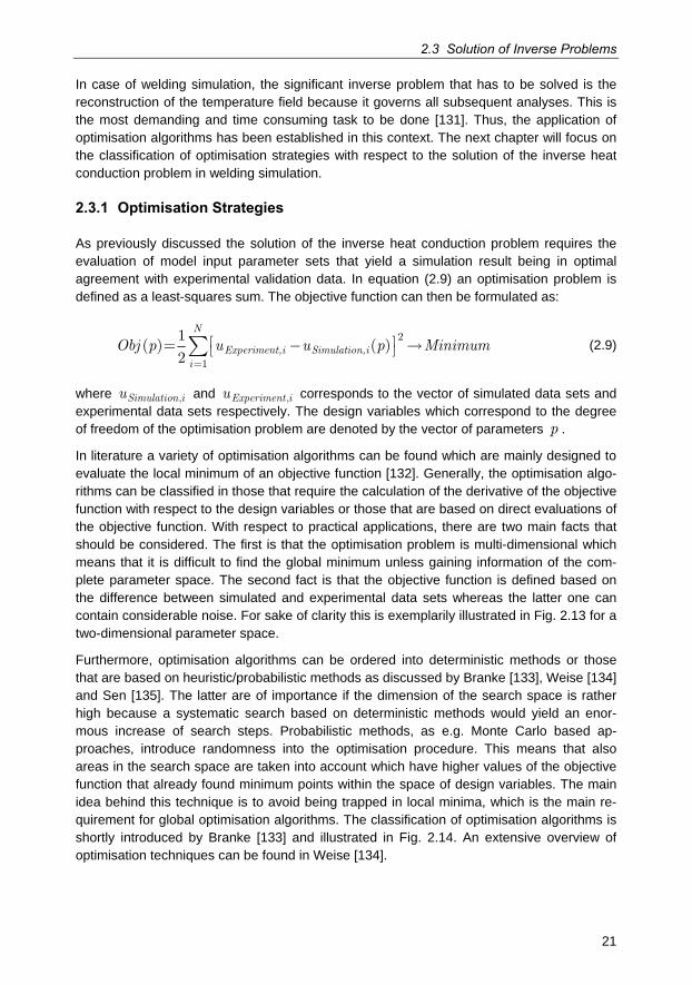
In literature a variety of optimisation algorithms can be found which are mainly designed to evaluate the local minimum of an objective function [132]. Generally, the optimisation algo-rithms can be classified in those that require the calculation of the derivative of the objective function with respect to the design variables or those that are based on direct evaluations of the objective function. With respect to practical applications, there are two main facts that should be considered. The first is that the optimisation problem is multi-dimensional which means that it is difficult to find the global minimum unless gaining information of the com-plete parameter space. The second fact is that the objective function is defined based on the difference between simulated and experimental data sets whereas the latter one can contain considerable noise. For sake of clarity this is exemplarily illustrated in Fig. 2.13 for a two-dimensional parameter space.
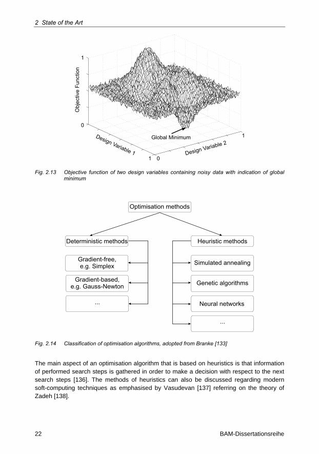
Furthermore, optimisation algorithms can be ordered into deterministic methods or those that are based on heuristic/probabilistic methods as discussed by Branke [133], Weise [134] and Sen [135]. The latter are of importance if the dimension of the search space is rather high because a systematic search based on deterministic methods would yield an enor-mous increase of search steps. Probabilistic methods, as e.g. Monte Carlo based ap-proaches, introduce randomness into the optimisation procedure. This means that also areas in the search space are taken into account which have higher values of the objective function that already found minimum points within the space of design variables. The main idea behind this technique is to avoid being trapped in local minima, which is the main re-quirement for global optimisation algorithms. The classification of optimisation algorithms is shortly introduced by Branke [133] and illustrated in Fig. 2.14. An extensive overview of optimisation techniques can be found in Weise [134].
2 State of the Art
22 BAM-Dissertationsreihe
Design Variable 1 Design Variable 2
Obj
ectiv
e Fu
nctio
n
Global Minimum
0
1
1 0
1
Fig. 2.13 Objective function of two design variables containing noisy data with indication of global minimum
Optimisation methods
Deterministic methods Heuristic methods
Simulated annealing
Genetic algorithms
Neural networks
Gradient-free,e.g. Simplex
Gradient-based,e.g. Gauss-Newton
...
...
Fig. 2.14 Classification of optimisation algorithms, adopted from Branke [133]
The main aspect of an optimisation algorithm that is based on heuristics is that information of performed search steps is gathered in order to make a decision with respect to the next search steps [136]. The methods of heuristics can also be discussed regarding modern soft-computing techniques as emphasised by Vasudevan [137] referring on the theory of Zadeh [138].
2.3 Solution of Inverse Problems
23
Back to global optimisation algorithms, heuristic procedures comprise simulated annealing, evolutionary methods or neural networks to name only the most known representatives.
Neural networks obey a structure that is closely related to the human brain [138], [139]. A neural network is constructed of neurons that are interacting by means of directed and weighted connections. The number and arrangement of simple information processing units (=neurons) governs the overall performance of such a network. The main capability of such a network of neurons is to solve problems which solutions can be described by examples (=pattern recognition). The training with respect to given patterns also enables to perform predictions for data sets that have not been part of the training data. This capability of a neural network is referred to as generalisation capability [140].
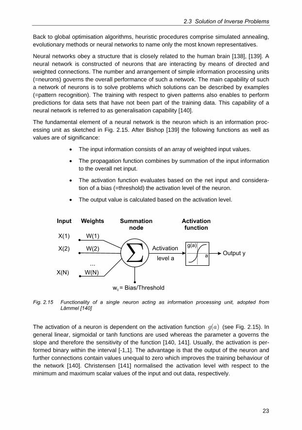
The fundamental element of a neural network is the neuron which is an information proc-essing unit as sketched in Fig. 2.15. After Bishop [139] the following functions as well as values are of significance:
The input information consists of an array of weighted input values.
The propagation function combines by summation of the input information to the overall net input.
The activation function evaluates based on the net input and considera-tion of a bias (=threshold) the activation level of the neuron.
The output value is calculated based on the activation level.
...
X(1)
X(2)
X(N)
Activation
level a a
g(a)
Activationfunction
Summationnode
W(1)
W(2)
W(N)
w = Bias/Threshold0
Output y
Input Weights
�
Fig. 2.15 Functionality of a single neuron acting as information processing unit, adopted from Lämmel [140]
The activation of a neuron is dependent on the activation function g a( ) (see Fig. 2.15). In general linear, sigmoidal or tanh functions are used whereas the parameter a governs the slope and therefore the sensitivity of the function [140, 141]. Usually, the activation is per-formed binary within the interval [-1,1]. The advantage is that the output of the neuron and further connections contain values unequal to zero which improves the training behaviour of the network [140]. Christensen [141] normalised the activation level with respect to the minimum and maximum scalar values of the input and out data, respectively.
2 State of the Art
24 BAM-Dissertationsreihe
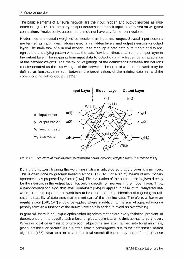
The basic elements of a neural network are the input, hidden and output neurons as illus-trated in Fig. 2.16. The property of input neurons is that their input is not based on weighted connections. Analogously, output neurons do not have any further connections.
Hidden neurons contain weighted connections as input and output. Several input neurons are termed as input layer, hidden neurons as hidden layers and output neurons as output layer. The main task of a neural network is to map input data onto output data and to rec-ognise the underlying pattern whereas the data flow is unidirectional from the input layer to the output layer. The mapping from input data to output data is achieved by an adaptation of the network weights. The matrix of weightings of the connections between the neurons can be denoted as the “knowledge” of the network. The error of a neural network may be defined as least-squares sum between the target values of the training data set and the corresponding network output [139].
W(1,1)
y (N )1 1
k=2
......
...
y (1)2
y (2)2
y (N )2 2
k=1y (1)1
x(1)
x(N )0
x(2)
w0
Input Layer Hidden Layer Output Layer
w0
x input vector
y output vector
W weight matrix
w bias vector0
W(i,j)
Fig. 2.16: Structure of multi-layered feed forward neural network, adopted from Christensen [141]
During the network training the weighting matrix is adjusted so that the error is minimised. This is often done by gradient based methods [142, 143] or even by means of evolutionary approaches as proposed by Kumar [144]. The evaluation of the output error is given directly for the neurons in the output layer but only indirectly for neurons in the hidden layer. Thus, a back-propagation algorithm after Rumelhart [145] is applied in case of multi-layered net-works. The training of the network has to be done under consideration of a good generali-sation capability of data sets that are not part of the training data. Therefore, a Bayesian regularisation [146, 147] should be applied where in addition to the sum of squared errors a penalty term as a function of the network weights is added to avoid an overtraining.
In general, there is no unique optimisation algorithm that solves every technical problem. In dependence on the specific task a local or global optimisation technique has to be chosen. Whereas local deterministic optimisation algorithms are also trapped into local minima’s, global optimisation techniques are often slow in convergence due to their stochastic search algorithm [135]. Near local minima the optimal search direction may not be found because
2.3 Solution of Inverse Problems
25
of the random design of such techniques [148]. In this context the publication of Neumaier [149] has to be emphasised since it comprises a comparison between various global opti-misation solvers. Janka [150] also discusses several stochastic optimisation algorithms. Furthermore, available software packages are tested with respect to mathematical test problems. Hedar [151] suggests the combination of local and global search paradigms as the combination of simulated annealing with direct search methods. Hedar [148] also dis-cusses the performance of an optimisation algorithm that uses a combination of simplex and genetic methods. Sutor [152] combines the Metropolis algorithm, which is a discrete stochastic method on that the simulated annealing method is based on, with a continuous direct optimisation method that originates on the steepest descent approach.
A further optimisation technique is the response surface methodology. Here, as a result of the scanning of the parameter space a response surface is calculated. This method is often used for technical optimisation problems as the design of experiments. An introduction to response surface methodology can be found in [153]. Further applications are presented by Marimuthu [154] and Balasubramanian [155]. Correia [156] compares the response surface methodology with genetic algorithms for evaluating optimal process parameters in GMAW.
Summarising it can be concluded that multidimensional problems require global optimisa-tion algorithms that analyse the entire domain of design variables. The efficient gain of knowledge about the sensitivity of the underlying process or model with respect to the de-sign variables is the key prerequisite in order to apply optimisation strategies efficiently. Since this information about the system to be optimised is difficult to obtain by a direct search approach, randomised methods are often chosen. Nevertheless, it has to be stressed that the overall optimisation efficiency can be enhanced significantly, if an optimi-sation pre-processing in terms of a multi-dimensional sensitivity study is performed. How-ever, in case of computational costly models or very inert systems this pre-processing is hardly to manage or very limited.
2.3.2 Applications for Welding Simulation
As introduced previously welding simulation comprises the solution of an inverse heat con-duction problem with the help of optimisation techniques. Therefore the definition of an appropriate objective function is necessary as proposed in equation (2.10).
[ ]N
i Simulation,i Experiment,ii 1
Obj p w u u MinimumN
21( ) ( )
=
= - å (2.10)
where simulationu corresponds to the vector of simulated data sets which is a function of the model parameters p and Experimentu to the vector of experimental reference data respec-tively. Equation (2.10) is set up as a L2-Norm which is used by Weiss [72] and Pittner [157] that also includes a weighting factor w that is set in dependence on the quality of experi-mental reference. The experimental data sets may be the fusion line in the cross section, the thermal cycles, microstructural properties, etc.
Karkhin [130] applies an objective function which is an augmented sum of square functions. The optimisation routine involves constraints (regularisation) of the design variables and
2 State of the Art
26 BAM-Dissertationsreihe
weighting factors. It is suggested to set the latter reciprocal to the variance of the measure-ment error. Here, the region of global minimum is detected by comparison of values of the objective function at different points. Subsequently, a Gauss-Newton method is employed to evaluate the optimal set of model parameters. Karkhin [158] also uses this optimisation strategy in order to evaluate the distribution of diffusible hydrogen during welding and cool-ing down.
Again, the knowledge about the global sensitivity of the model is of importance to choose the appropriate design variables. Gabriel [159] applies a global sensitivity analysis for the numerical modelling of the temperature field in narrow gap gas tungsten arc (GTA) welding. The model contains about 10 parameters given by the double ellipsoidal heat source (5 parameters), side wall boundary condition by parabolic parietal heat sources (3 parame-ters) and NEWTON’S law at the top and bottom surface (2 parameters). This requires a multi-variable optimisation technique. The objective function is set up as a least squares sum of measured and calculated weld characteristics. Furthermore, a sensitivity analysis is per-formed by evaluating the influence of a parameter variation on the temperature field. It is concluded that if the sensitivity is high then the parameter is well suited as tuning parameter (=design variable). However, the possibility of having an ill-posed problem has also to be taken into account because this would worsen the calibration behaviour of the model.
The solution of an inverse problem by means of direct simulations requires dozens of calcu-lations to be performed. Therefore, the computational cost of the direct simulation model is an important issue. Concerning this matter Weiss [80] and Kumar [86] applied meta models which are neural network approximations of the underlying temperature field model. The neural network is trained with model input parameters and the corresponding simulation results. In [86] fillet welds are considered with penetration, throat, leg length as experimen-tal weld characteristics and arc efficiency, radius of cylindrical source and enhanced ther-mal conductivity are considered as model input. The trained neural network is capable of performing 4000 iterations within 6 minutes on an ordinary office PC. Nevertheless, the following facts have to be emphasised. One is that many simulations have to be done in advance in order to provide training data. In case of numerically intensive models this yields high computational requirements. In addition, if the problem setup is changed, e.g. geome-try, the network has to be trained again since the meta-model can only be used for a spe-cific problem setup. Finally, if more weld characteristics should be considered as a thermal cycle the number of output variables increases and therefore the network training is more sophisticated [139]. Similar approaches of applying meta-models in the context of enabling fast direct simulations are also presented by Nandan [160] and Jin [161].
With respect to optimisation algorithms that are taken for solving the inverse problem in welding simulation various methods are present. Kumar [86, 162] and De [163, 164] employ a deterministic search method as a conjugate gradient method and LEVENBERG-MARQUADT algorithm to solve the multi-parameter problem. The design variables are the arc efficiency, radius of cylindrical heat source and effective thermal conductivity. The response variables are penetration depth, leg length and throat depth. The objective function is defined as least squares difference between simulated and measured values. The experimental reference data include 5 sets. The objective function is set up as a sum of least squares between calculated and measured weld characteristics that are evaluated from the seam shape and defined as the sum over all experiments. Therefore, the calibrated model should fit in the
2.3 Solution of Inverse Problems
27
mean for all considered experiments. The main aspect with regards to local optimisation algorithms is emphasised here as well, namely the need for the definition of an initial start value that governs the ability of the optimisation algorithm to detect the global minimum or being trapped in local minima. This has to be done a priori and is dependent on the knowl-edge and capability of the human user. Furthermore, various combinations of model pa-rameters (design variables) may yield the same output, so that the optimisation problem can be denoted as multi-valued.
The difference between direct optimisation schemes as the conjugate gradient method and global ones like genetic algorithms with regards to the neural network training is extensively discussed by Kumar [144]. The combination of local and global optimisation methodologies is done by using the conjugate gradient method to perform ten optimisation runs for differ-ent start points. The obtained local minima are taken as initial population for the genetic algorithms.
Kumar [165] and Bag [166] take the fact of a possible multi-valued character of objective functions into account and apply a genetic algorithm to solve the inverse heat conduction problem. Again, a meta-model of a numerical temperature field model that also includes hydrodynamics is used in terms of a neural network to reduce the time needed for the direct simulations. The problem to be examined considers the fusion line in the cross section of gas metal arc (GMA) fillet weld joints which is governed by penetration depth, throat and leg length as well as current, voltage, welding speed and wire feed rate as design variables. The application of the genetic algorithm includes the following steps. Firstly, an initial popu-lation has to be defined to represent the variable space sufficiently. The genetic operators recombination, cross over and mutation are applied iteratively and as a result the diversity of the population decreases. Therefore, the solution starts crowding at specific regions of the model space. The end population comprises 8 sets of parameters having minimum values of the objective function. Further applications of genetic algorithms for multi-variable optimisation are also presented by [167, 168]
Jeberg [169] analyses the inverse problem in connection with the modelling of GMA weld-ing of 5 mm thick steel plates. He solves the temperature field based on a finite element model and calculates the weld pool surface depression subsequently. The objective func-tion is defined as least squares sum of calculated and measured geometry of the fusion line in the cross section and the thermal cycles. The space of adjustable model parameters involves 6 dimensions that are spanned by the 4 heat intensity distribution parameters of the top Goldak heat source plus its power as well as the overall heat input under considera-tion of an additional box-shaped internal heat source. The search space consequently has 6 dimensions. The space of process parameters contains the arc voltage and current which are combined to the net power and the welding velocity. Furthermore, the surface depres-sion model is calibrated as well by searching for the optimal configuration of the three model parameters which are surface tension, arc pressure and arc pressure distribution. The sequential calibration of two sub-models is done using the deterministic local optimisa-tion approach that is based on a sequential quadratic programming technique. It is argued that if the calibration was performed only against single experiments the prediction capabil-ity of the model within the process parameter space is limited because it is only valid in a small neighbourhood around the calibration point. In addition, an approach to manage the calibration results for multiple, in this case 9 experiments is presented. 4 calibration points
2 State of the Art
28 BAM-Dissertationsreihe
are selected to define the process parameter space. This rectangle is treated as an isoparametric finite element whereas the nodal values correspond to the process parameter sets. An interpolation between the nodal values is performed by a bilinear approach. The calibration against multiple experiments and processing of the calibration and extension of the model validity range by interpolation is shown in more detail in [170]. However, since the relationship between model parameters and process parameters is non-linear it is ques-tionable whether a bilinear interpolation over a wide range of the process parameter is always feasible. Furthermore, this approach requires two or three dimensional process parameter spaces. In this context the question arises how multi-dimensional parameter spaces can be treated.
Okui [171] applies a moving point source to calculate the pool width and depth. The sys-tematic deviation with regards to performed experiments is analyzed by a regression model on the basis of exponential fitting functions. In general, the model is not extended or tuned because only the model response is adjusted by a post regression analysis.
Erofeev [172] solves the inverse problem and links the process parameters such as welding speed and beam power to the bead geometry by using a linear relationship between the geometry parameters and the process parameters yielding a system of linear equations. With respect to the calibration of the numerical model it has to be considered that various combinations of the power and welding speed can yield the same cross section.
Goncalves [173] applies a simulated annealing and golden section approach to calibrate the model against validation data. The inverse problem is decomposed into a sequence of direct problems by applying two different models: an analytical line source model and a finite volume discretisation taking the effect of latent heat into account. If the analytical model is employed then the global simulated annealing algorithm is used because it allows performing dozens of direct simulation within less computation time. In case of the numeri-cal model, which is orders of magnitudes slower than the analytical model, the golden search method is utilised to find the optimal model parameter set that minimises the objec-tive function. A further contribution can be found in [174].
Ferrari [175] uses an analytical model to simulate the temperature distribution that occurs during quenching. He interprets the inverse problem as a sequence of direct solutions that have to be solved. Lambrakos [176, 177, 178] also discusses different approaches to solve inverse problems in heat deposition processes and offers a detailed overview of recent advances and techniques of solving inverse problems.
Summarising, it can be stated that on the one hand welding simulation is based on phe-nomenological models which represent a rough approximation of the real process. The simplification yields that the relationship between model input parameters and the real process parameters are not known in advance. This requires the calibration of the welding simulation against experimental data which can be denoted in mathematical terms as an inverse problem. Since the parameter space is multidimensional, deterministic search algo-rithms are less applicable due to being trapped in local minima or the requirement of per-forming an unacceptable amount of direct simulations. Therefore, stochastic methods came into play as simulated annealing and genetic algorithms or the heuristic modelling based on neural networks. Especially the latter aspect is of importance in the field describing and analysing complex systems as the welding process. This so called “soft-computing” was
2.3 Solution of Inverse Problems
29
firstly introduced by Zadeh [138] approximately 20 years ago and refers to the way of solv-ing problems like human beings which are imprecise in some way but more effective as precise approaches. One of the outmost significant and most often “soft-computing” method is the utilisation of artificial neural networks. They are used where the mathematical formu-lation of the problem is too complex and are often referred to as “black-box” modelling. Applications can be found in the field of control of the welding process with respect to stabil-ity as well as the obtained weld characteristics [141, 161, 179-181].
Concluding it can be said, that the efficient solution of the temperature field requires two prerequisites to be fulfilled. The first is to provide a fast solution to the temperature field in order to enable the application of optimisation algorithms. The second need is related to the optimisation itself. Due to the multidimensionality of the inverse heat conduction problem in welding simulation the usage of global optimisation schemes is preferable. However, a sufficient optimisation requires knowledge regarding the process. In other words, the sensi-tivity of the heat source energy distribution regarding the temperature field has to be known. This allows an appropriate setup of the domain of design variables. In this context, the possible occurrence of several local minima, which is often referred to as multi-valued char-acter, of the objective function to be analysed. Here the influence of the experimental data on the shape of the objective function and characteristic of the global minimum needs to be examined that enables to evaluate which characteristics of the temperature field have to be known to describe it uniquely.
Another field of interest ought to be the derivation of an appropriate initial set of parameters within the design space of the model that reduces the amount of direct search steps. Goldak [93] proposed the direct relation of the seam geometry to a corresponding energy distribution. This suggestion is still applied today, like in [182]. A further geometric derivation of energy distribution with the fusion zone as input data has been applied for a US patent by Zhang [94]. However, since all these approaches do not account for specific welding processes in terms of different energy distributions, the dimensionality of heat conduction mode or travelling speed of the heat source has to be incorporated. Hence, the develop-ment of a more physical approach to derive an energy distribution of a volume heat source directly from the fusion zone is needed. The reduction of complexity of the global optimisa-tion problem (=dimension of design variables space) and to provide a sufficient initial set of model parameters appears to be essential for the efficient solution of the inverse heat con-duction problem in welding simulation.
30 BAM-Dissertationsreihe
3 Execution of Experiments
This chapter describes the experimental as well as computational investigations that were conducted. The aim of the following analyses is to act on the statements of the previous chapter concerning the solution of the inverse heat conduction problem in welding simula-tion. Referring to this, the general conclusion can be drawn that two major aspects govern the inverse problem solution. In particular, this is the computational effort of the phenome-nological model and the efficiency of the optimisation algorithm. Consequently, the present work focuses on the development of fast solutions to the temperature field and the applica-tion of a global optimisation algorithm. Here, only the reconstruction of the temperature field on basis of experimental reference data will be examined. Subsequent analyses like themomechanical calculations will not be the subject of this work. Furthermore, the influ-ence of the temperature independence of the material data will not be discussed. Here, the agreement with the experimental reference data governs the applicability of the used mod-elling approach.
3.1 Experimental Investigations
The paragraph is dedicated to the experimental investigations in order to provide the refer-ence data for which the simulation model is calibrated against. The specimen that is used for all the welding experiments is a plate of the dimensions as shown in Fig. 3.1. The weld-ing trajectory is a linear path. An I-joint butt weld with milled edges and a gap-width of tech-nical zero is taken into account.
In order to obtain the needed reference data thermo couple measurements at the top and bottom surface are done. The thermo couples that are used have a diameter of 0.13 mm and are of type K (Ni/CrNi). The sampling rate for the temperature measurements was set to 150 Hz. In addition to that, the fusion line in the cross section is evaluated by taking macro sections in the region where the thermo couples have been placed. The geometry of the top weld pool is evaluated by means of a high-speed camera
The main requirement that has to ensured is that the capability to solve the inverse heat conduction problem must be independent on the welding process or material under study. Therefore, various welding techniques are employed that obey differences in the heat input and consequently significantly different weld seams. In particular, these are laser beam welding experiments by usage of a 20 kW fibre laser and laser-gas metal arc hybrid welds by a combination of the 20 kW fibre laser with a pulsed arc welding process. While the laser welding process incorporates high spatial and temporal gradients the laser-arc hybrid proc-ess involves high gradients in the laser dominated region and less steep gradients at the top surface where the arc is dominant. Furthermore, the molten pool is significantly larger for the laser-arc hybrid process as for the laser beam welding process.
The experiments are done for the steel S355J2+N which is taken for the numerical as well as the experimental investigations. The chemical composition of the hot rolled mild steel
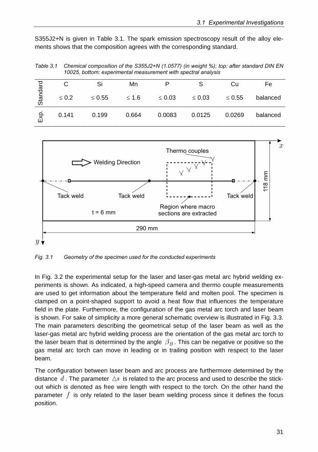
3.1 Experimental Investigations
31
S355J2+N is given in Table 3.1. The spark emission spectroscopy result of the alloy ele-ments shows that the composition agrees with the corresponding standard.
Table 3.1 Chemical composition of the S355J2+N (1.0577) (in weight %); top: after standard DIN EN 10025, bottom: experimental measurement with spectral analysis
Sta
ndar
d
C Si Mn P S Cu Fe
0.2 0.55 1.6 0.03 0.03 0.55 balanced
Exp
.
0.141 0.199 0.664 0.0083 0.0125 0.0269 balanced
290 mm
118
mm
Tack weld Tack weld Tack weld
Thermo couples
Region where macrosections are extracted
y
x
Welding Direction
t = 6 mm
Fig. 3.1 Geometry of the specimen used for the conducted experiments
In Fig. 3.2 the experimental setup for the laser and laser-gas metal arc hybrid welding ex-periments is shown. As indicated, a high-speed camera and thermo couple measurements are used to get information about the temperature field and molten pool. The specimen is clamped on a point-shaped support to avoid a heat flow that influences the temperature field in the plate. Furthermore, the configuration of the gas metal arc torch and laser beam is shown. For sake of simplicity a more general schematic overview is illustrated in Fig. 3.3. The main parameters describing the geometrical setup of the laser beam as well as the laser-gas metal arc hybrid welding process are the orientation of the gas metal arc torch to the laser beam that is determined by the angle Bb . This can be negative or positive so the gas metal arc torch can move in leading or in trailing position with respect to the laser beam.
The configuration between laser beam and arc process are furthermore determined by the distance d . The parameter s is related to the arc process and used to describe the stick-out which is denoted as free wire length with respect to the torch. On the other hand the parameter f is only related to the laser beam welding process since it defines the focus position.
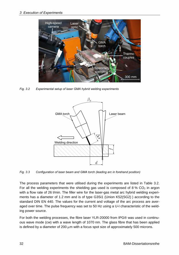
3 Execution of Experiments
32 BAM-Dissertationsreihe
Fig. 3.2 Experimental setup of laser GMA hybrid welding experiments
d
�B
�s
Welding direction
GMA torchf
Laser beam
Fig. 3.3 Configuration of laser beam and GMA torch (leading arc in forehand position)
The process parameters that were utilised during the experiments are listed in Table 3.2. For all the welding experiments the shielding gas used is composed of 8 % CO2 in argon with a flow rate of 26 l/min. The filler wire for the laser-gas metal arc hybrid welding experi-ments has a diameter of 1.2 mm and is of type G3Si1 (Union K52(SG2) ) according to the standard DIN EN 440. The values for the current and voltage of the arc process are aver-aged over time. The pulse frequency was set to 50 Hz using a U-I characteristic of the weld-ing power source.
For both the welding processes, the fibre laser YLR-20000 from IPG® was used in continu-ous wave mode (cw) with a wave length of 1070 nm. The glass fibre that has been applied is defined by a diameter of 200 m with a focus spot size of approximately 500 microns.
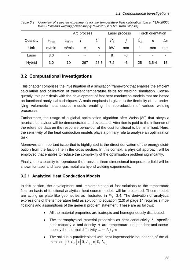
3.2 Computational Investigations
33
Table 3.2 Overview of selected experiments for the temperature field calibration (Laser YLR-20000 from IPG® and welding power supply “Quinto” GLC 603 from Cloos®)
Arc process Laser process Torch orientation
Quantity vWeld vWire I U PL f bB d s
Unit m/min m/min A V kW mm ° mm mm
Laser 3.0 - - - 8 -6 - - -
Hybrid 3.0 10 267 26.5 7.2 -6 25 3.5-4 15
3.2 Computational Investigations
This chapter comprises the investigation of a simulation framework that enables the efficient calculation and calibration of transient temperature fields for welding simulation. Conse-quently, this part deals with the development of fast heat conduction models that are based on functional-analytical techniques. A main emphasis is given to the flexibility of the under-lying volumetric heat source models enabling the reproduction of various welding processes.
Furthermore, the usage of a global optimisation algorithm after Weiss [80] that obeys a heuristic behaviour will be demonstrated and evaluated. Attention is paid to the influence of the reference data on the response behaviour of the cost functional to be minimised. Here, the sensitivity of the heat conduction models plays a primary role to analyse an optimisation task.
Moreover, an important issue that is highlighted is the direct derivation of the energy distri-bution from the fusion line in the cross section. In this context, a physical approach will be employed that enables to reduce the complexity of the optimisation problem significantly.
Finally, the capability to reproduce the transient three dimensional temperature field will be shown for laser and laser-gas metal arc hybrid welding experiments.
3.2.1 Analytical Heat Conduction Models
In this section, the development and implementation of fast solutions to the temperature field on basis of functional-analytical heat source models will be presented. These models are acting on plate like geometries as illustrated in Fig. 3.4. The derivation of analytical expressions of the temperature field as solution to equation (2.3) at page 14 requires simpli-fications and assumptions of the general problem statement. These are as follows:
All the material properties are isotropic and homogeneously distributed.
The thermophysical material properties as heat conductivity l , specific heat capacity c and density r are temperature independent and conse-quently the thermal diffusivity a cl r= .
The solid is a parallelepiped with heat impermeable boundaries of the di-mension xL0,é ùë û x yL0,é ùë û x zL0,é ùë û
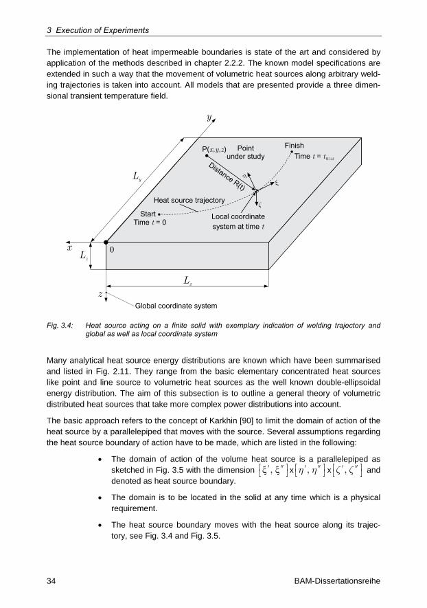
3 Execution of Experiments
34 BAM-Dissertationsreihe
The implementation of heat impermeable boundaries is state of the art and considered by application of the methods described in chapter 2.2.2. The known model specifications are extended in such a way that the movement of volumetric heat sources along arbitrary weld-ing trajectories is taken into account. All models that are presented provide a three dimen-sional transient temperature field.
P( )x,y,z Pointunder study
Distance R(t)
Heat source trajectory
Local coordinatesystem at time t
StartTime = 0t
FinishTime =t tWeld
y
x
Ly
Lz
z
Lx
0
Global coordinate system
�
�
�
Fig. 3.4: Heat source acting on a finite solid with exemplary indication of welding trajectory and global as well as local coordinate system
Many analytical heat source energy distributions are known which have been summarised and listed in Fig. 2.11. They range from the basic elementary concentrated heat sources like point and line source to volumetric heat sources as the well known double-ellipsoidal energy distribution. The aim of this subsection is to outline a general theory of volumetric distributed heat sources that take more complex power distributions into account.
The basic approach refers to the concept of Karkhin [90] to limit the domain of action of the heat source by a parallelepiped that moves with the source. Several assumptions regarding the heat source boundary of action have to be made, which are listed in the following:
The domain of action of the volume heat source is a parallelepiped as sketched in Fig. 3.5 with the dimension ξ ξ,¢ é ùë û x ,h h¢ é ùë û x ,z z¢ é ùë û and denoted as heat source boundary.
The domain is to be located in the solid at any time which is a physical requirement.
The heat source boundary moves with the heat source along its trajec-tory, see Fig. 3.4 and Fig. 3.5.
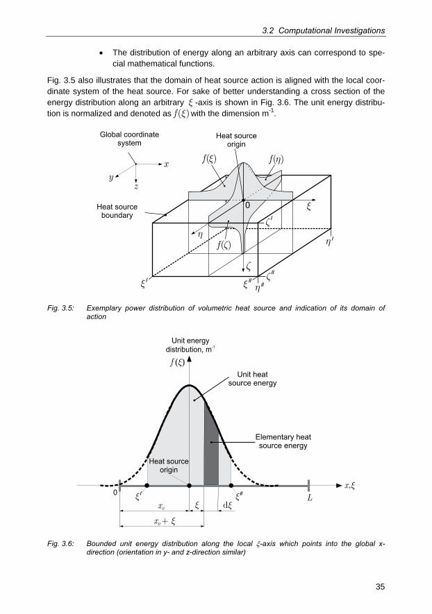
3.2 Computational Investigations
35
The distribution of energy along an arbitrary axis can correspond to spe-cial mathematical functions.
Fig. 3.5 also illustrates that the domain of heat source action is aligned with the local coor-dinate system of the heat source. For sake of better understanding a cross section of the energy distribution along an arbitrary x -axis is shown in Fig. 3.6. The unit energy distribu-tion is normalized and denoted as f ( )x with the dimension m-1.
f( )� f( )�
�/ //
� � /
/�
//�
�
Heat sourceorigin
z
x
y
Global coordinatesystem
�/
f( )�
Heat sourceboundary
�
�
0
/
Fig. 3.5: Exemplary power distribution of volumetric heat source and indication of its domain of action
Unit energydistribution, m-1
� d�x0
x0 + �
0L
Heat sourceorigin
f ( )�
x,�
� / � //
Unit heatsource energy
Elementary heatsource energy
Fig. 3.6: Bounded unit energy distribution along the local -axis which points into the global x-direction (orientation in y- and z-direction similar)
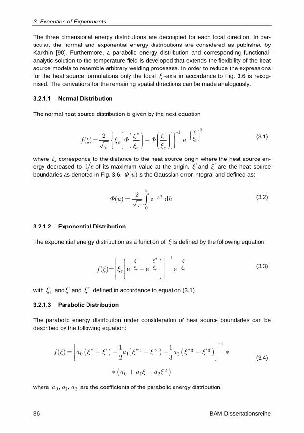
3 Execution of Experiments
36 BAM-Dissertationsreihe
The three dimensional energy distributions are decoupled for each local direction. In par-ticular, the normal and exponential energy distributions are considered as published by Karkhin [90]. Furthermore, a parabolic energy distribution and corresponding functional-analytic solution to the temperature field is developed that extends the flexibility of the heat source models to resemble arbitrary welding processes. In order to reduce the expressions for the heat source formulations only the local x -axis in accordance to Fig. 3.6 is recog-nised. The derivations for the remaining spatial directions can be made analogously.
3.2.1.1 Normal Distribution
The normal heat source distribution is given by the next equation
eee e
f
2-1'' '2
( ) exxx x
x x F Fx xp
æ ö÷ç- ÷ç ÷÷çè øì é æ ö æ öù üï ïï ï÷ ÷ç ç= ê - ú÷ ÷í ýç ç÷ ÷ç çï ïê è ø è øúï ïî ë û þ
(3.1)
where ex corresponds to the distance to the heat source origin where the heat source en-ergy decreased to e1 of its maximum value at the origin. 'x and ''x are the heat source boundaries as denoted in Fig. 3.6. u( )F is the Gaussian error integral and defined as:
u
hu h2
0
2( ) e dF
p-= ò (3.2)
3.2.1.2 Exponential Distribution
The exponential energy distribution as a function of x is defined by the following equation
e e eef
' '' 1
( ) e e ex x xx x xx x
-- - -é æ ö ù÷çê ú÷ç= - ÷çê ú÷ç ÷÷çê úè øë û
(3.3)
with ex and 'x and ''x defined in accordance to equation (3.1).
3.2.1.3 Parabolic Distribution
The parabolic energy distribution under consideration of heat source boundaries can be described by the following equation:
( ) ( ) ( )
( )
f a a a
a a a
1
'' ' '' 2 '2 '' 3 ' 30 1 2
20 1 2
1 1( )
2 3x x x x x x x
x x
-é ù= ê - + - + - ú *
ê úë û
* + +
(3.4)
where a a a0 1 2, , are the coefficients of the parabolic energy distribution.
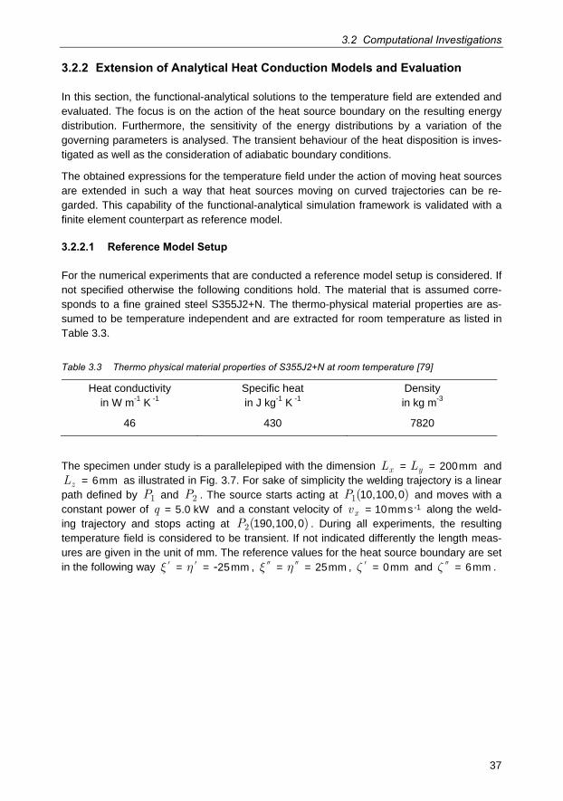
3.2 Computational Investigations
37
3.2.2 Extension of Analytical Heat Conduction Models and Evaluation
In this section, the functional-analytical solutions to the temperature field are extended and evaluated. The focus is on the action of the heat source boundary on the resulting energy distribution. Furthermore, the sensitivity of the energy distributions by a variation of the governing parameters is analysed. The transient behaviour of the heat disposition is inves-tigated as well as the consideration of adiabatic boundary conditions.
The obtained expressions for the temperature field under the action of moving heat sources are extended in such a way that heat sources moving on curved trajectories can be re-garded. This capability of the functional-analytical simulation framework is validated with a finite element counterpart as reference model.
3.2.2.1 Reference Model Setup
For the numerical experiments that are conducted a reference model setup is considered. If not specified otherwise the following conditions hold. The material that is assumed corre-sponds to a fine grained steel S355J2+N. The thermo-physical material properties are as-sumed to be temperature independent and are extracted for room temperature as listed in Table 3.3.
Table 3.3 Thermo physical material properties of S355J2+N at room temperature [79]
Heat conductivity in W m-1 K -1
Specific heat in J kg-1 K -1
Density in kg m-3
46 430 7820
The specimen under study is a parallelepiped with the dimension x yL L= = 200mm and
zL = 6mm as illustrated in Fig. 3.7. For sake of simplicity the welding trajectory is a linear path defined by P1 and P2 . The source starts acting at P1( )10,100,0 and moves with a constant power of q = 5.0 kW and a constant velocity of xv -1= 10mms along the weld-ing trajectory and stops acting at P2( )190,100,0 . During all experiments, the resulting temperature field is considered to be transient. If not indicated differently the length meas-ures are given in the unit of mm. The reference values for the heat source boundary are set in the following way x h¢ ¢= = 25mm- , x h = = 25mm , z ¢ = 0mm and z = 6mm .
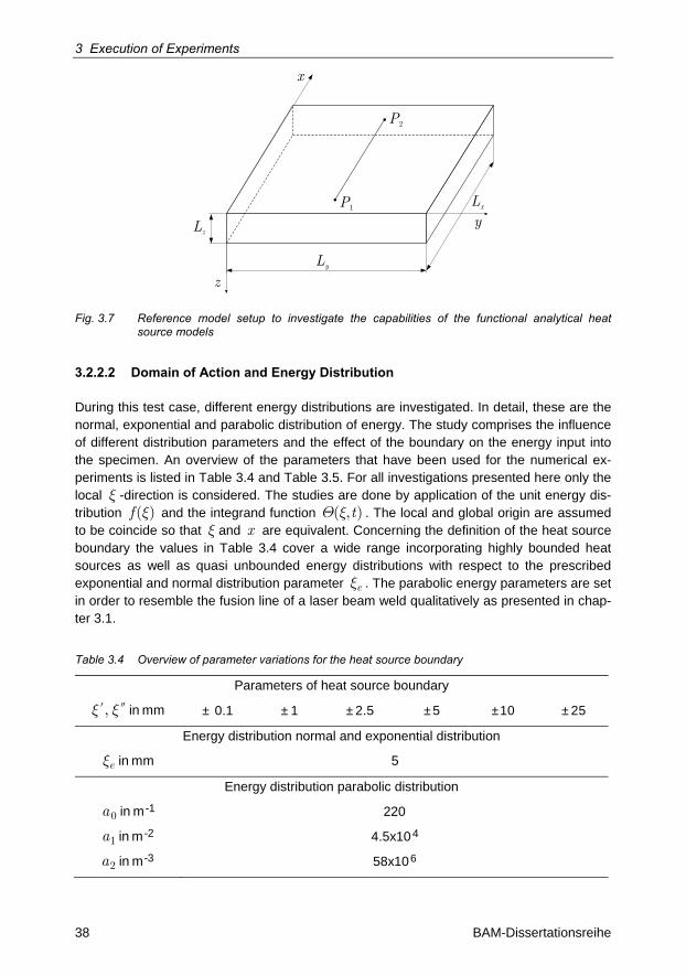
3 Execution of Experiments
38 BAM-Dissertationsreihe
Lz
Ly
P1
P2
x
y
z
Lx
Fig. 3.7 Reference model setup to investigate the capabilities of the functional analytical heat source models
3.2.2.2 Domain of Action and Energy Distribution
During this test case, different energy distributions are investigated. In detail, these are the normal, exponential and parabolic distribution of energy. The study comprises the influence of different distribution parameters and the effect of the boundary on the energy input into the specimen. An overview of the parameters that have been used for the numerical ex-periments is listed in Table 3.4 and Table 3.5. For all investigations presented here only the local x -direction is considered. The studies are done by application of the unit energy dis-tribution f ( )x and the integrand function t( , )Q x . The local and global origin are assumed to be coincide so that x and x are equivalent. Concerning the definition of the heat source boundary the values in Table 3.4 cover a wide range incorporating highly bounded heat sources as well as quasi unbounded energy distributions with respect to the prescribed exponential and normal distribution parameter ex . The parabolic energy parameters are set in order to resemble the fusion line of a laser beam weld qualitatively as presented in chap-ter 3.1.
Table 3.4 Overview of parameter variations for the heat source boundary
Parameters of heat source boundary
,x x¢ in mm ± 0.1 ± 1 ± 2.5 ± 5 ±10 ± 25
Energy distribution normal and exponential distribution
ex in mm 5
Energy distribution parabolic distribution
a0-1in m 220
a1-2in m 44.5x10
a2-3in m 658x10
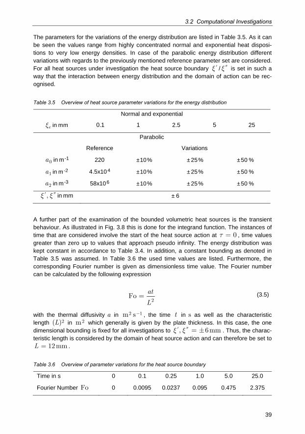
3.2 Computational Investigations
39
The parameters for the variations of the energy distribution are listed in Table 3.5. As it can be seen the values range from highly concentrated normal and exponential heat disposi-tions to very low energy densities. In case of the parabolic energy distribution different variations with regards to the previously mentioned reference parameter set are considered. For all heat sources under investigation the heat source boundary x ¢ / x is set in such a way that the interaction between energy distribution and the domain of action can be rec-ognised.
Table 3.5 Overview of heat source parameter variations for the energy distribution
Normal and exponential
ex in mm 0.1 1 2.5 5 25
Parabolic
Reference Variations
a0-1in m 220 ±10% ± 25% ±50 %
a1-2in m 44.5x10 ±10% ± 25% ±50 %
a2-3in m 658x10 ±10% ± 25% ±50 %
,x x¢ in mm ± 6
A further part of the examination of the bounded volumetric heat sources is the transient behaviour. As illustrated in Fig. 3.8 this is done for the integrand function. The instances of time that are considered involve the start of the heat source action at 0t = , time values greater than zero up to values that approach pseudo infinity. The energy distribution was kept constant in accordance to Table 3.4. In addition, a constant bounding as denoted in Table 3.5 was assumed. In Table 3.6 the used time values are listed. Furthermore, the corresponding Fourier number is given as dimensionless time value. The Fourier number can be calculated by the following expression
at
L2Fo = (3.5)
with the thermal diffusivity a in 2 1m s- , the time t in s as well as the characteristic length L 2( ) in 2m which generally is given by the plate thickness. In this case, the one dimensional bounding is fixed for all investigations to , 6mmx x¢ = . Thus, the charac-teristic length is considered by the domain of heat source action and can therefore be set to L 12mm= .
Table 3.6 Overview of parameter variations for the heat source boundary
Time in s 0 0.1 0.25 1.0 5.0 25.0
Fourier Number Fo 0 0.0095 0.0237 0.095 0.475 2.375
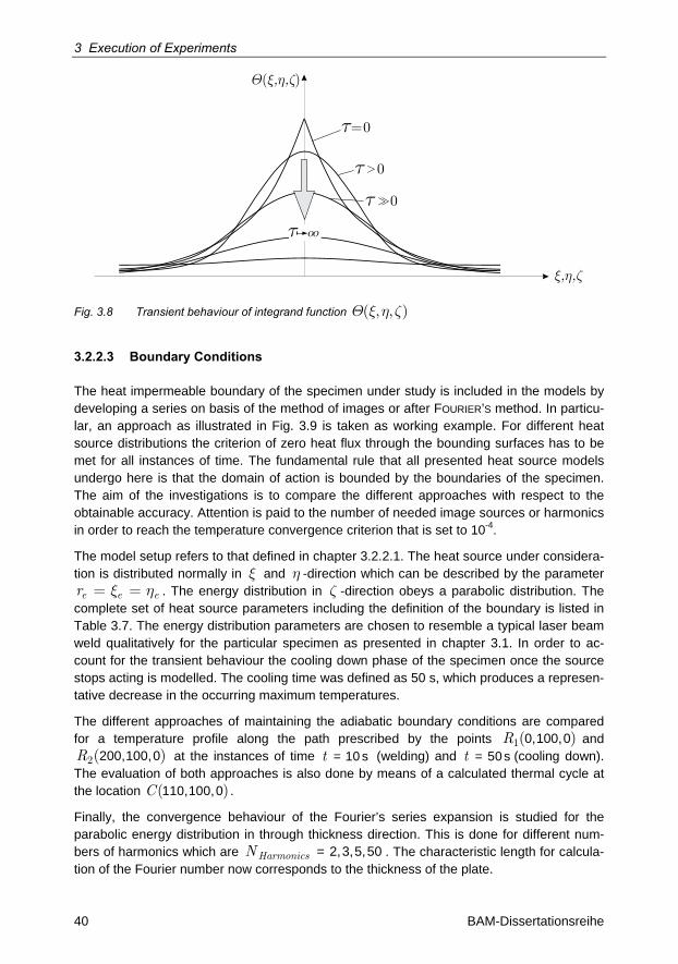
3 Execution of Experiments
40 BAM-Dissertationsreihe
� � �, ,
�=0
� �����( )
�
� 0�
� 0�
Fig. 3.8 Transient behaviour of integrand function ( , , )Q x h z
3.2.2.3 Boundary Conditions
The heat impermeable boundary of the specimen under study is included in the models by developing a series on basis of the method of images or after FOURIER’S method. In particu-lar, an approach as illustrated in Fig. 3.9 is taken as working example. For different heat source distributions the criterion of zero heat flux through the bounding surfaces has to be met for all instances of time. The fundamental rule that all presented heat source models undergo here is that the domain of action is bounded by the boundaries of the specimen. The aim of the investigations is to compare the different approaches with respect to the obtainable accuracy. Attention is paid to the number of needed image sources or harmonics in order to reach the temperature convergence criterion that is set to 10-4.
The model setup refers to that defined in chapter 3.2.2.1. The heat source under considera-tion is distributed normally in x and h -direction which can be described by the parameter
e e er x h= = . The energy distribution in z -direction obeys a parabolic distribution. The complete set of heat source parameters including the definition of the boundary is listed in Table 3.7. The energy distribution parameters are chosen to resemble a typical laser beam weld qualitatively for the particular specimen as presented in chapter 3.1. In order to ac-count for the transient behaviour the cooling down phase of the specimen once the source stops acting is modelled. The cooling time was defined as 50 s, which produces a represen-tative decrease in the occurring maximum temperatures.
The different approaches of maintaining the adiabatic boundary conditions are compared for a temperature profile along the path prescribed by the points R1( )0,100,0 and R2( )200,100,0 at the instances of time t = 10 s (welding) and t = 50 s (cooling down). The evaluation of both approaches is also done by means of a calculated thermal cycle at the location C( )110,100,0 .
Finally, the convergence behaviour of the Fourier’s series expansion is studied for the parabolic energy distribution in through thickness direction. This is done for different num-bers of harmonics which are HarmonicsN = 2,3,5,50 . The characteristic length for calcula-tion of the Fourier number now corresponds to the thickness of the plate.
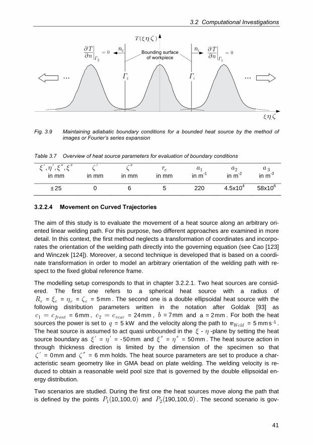
3.2 Computational Investigations
41
T( )�, ,� �
Tn
1
0
���
Tn
2
0
���
n1n2 Bounding surfaceof workpiece
� �
�, ,� �
......
Fig. 3.9 Maintaining adiabatic boundary conditions for a bounded heat source by the method of images or Fourier’s series expansion
Table 3.7 Overview of heat source parameters for evaluation of boundary conditions
, , ,x h x x¢ ¢ in mm
z ¢ in mm
z in mm
er in mm
a1 in m-1
a2 in m-2
a 3 in m-3
± 25 0 6 5 220 4.5x10⁴ 58x106
3.2.2.4 Movement on Curved Trajectories
The aim of this study is to evaluate the movement of a heat source along an arbitrary ori-ented linear welding path. For this purpose, two different approaches are examined in more detail. In this context, the first method neglects a transformation of coordinates and incorpo-rates the orientation of the welding path directly into the governing equation (see Cao [123] and Winczek [124]). Moreover, a second technique is developed that is based on a coordi-nate transformation in order to model an arbitrary orientation of the welding path with re-spect to the fixed global reference frame.
The modelling setup corresponds to that in chapter 3.2.2.1. Two heat sources are consid-ered. The first one refers to a spherical heat source with a radius of
e e e eR x h z= = = = 5mm . The second one is a double ellipsoidal heat source with the following distribution parameters written in the notation after Goldak [93] as
frontc c1 = = 6mm , rearc c2 = = 24mm , b = 7mm and a = 2mm . For both the heat sources the power is set to q = 5 kW and the velocity along the path to Weldv -1= 5 mm s . The heat source is assumed to act quasi unbounded in the x h- -plane by setting the heat source boundary as x h¢ ¢= = -50mm and x h = = 50mm . The heat source action in through thickness direction is limited by the dimension of the specimen so that z ¢ = 0mm and z = 6 mm holds. The heat source parameters are set to produce a char-acteristic seam geometry like in GMA bead on plate welding. The welding velocity is re-duced to obtain a reasonable weld pool size that is governed by the double ellipsoidal en-ergy distribution.
Two scenarios are studied. During the first one the heat sources move along the path that is defined by the points P1( )10,100,0 and P2( )190,100,0 . The second scenario is gov-
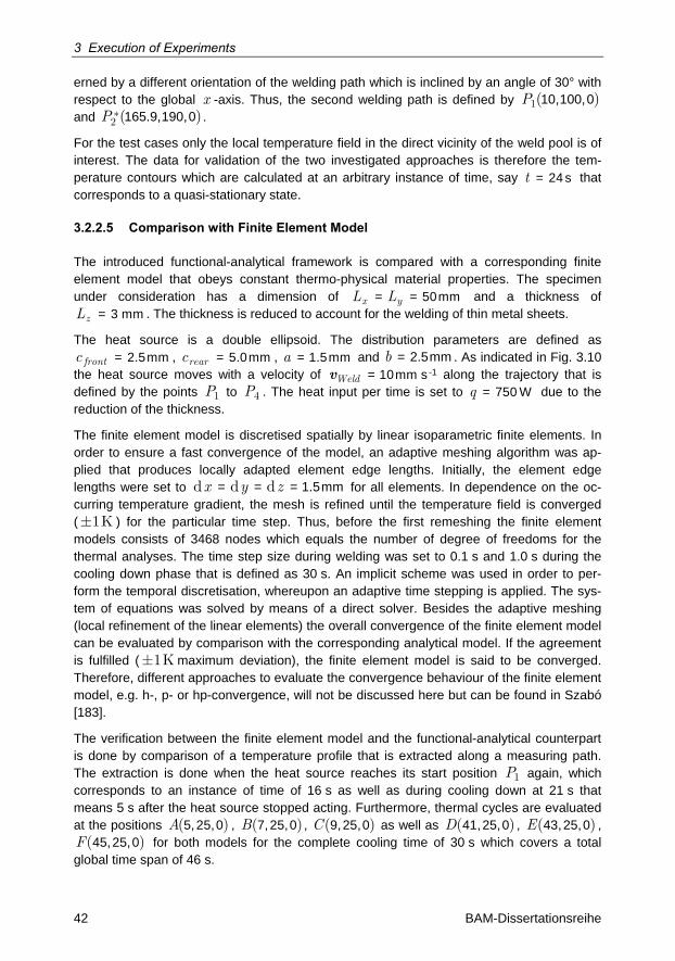
3 Execution of Experiments
42 BAM-Dissertationsreihe
erned by a different orientation of the welding path which is inclined by an angle of 30° with respect to the global x -axis. Thus, the second welding path is defined by P1( )10,100,0 and P2 ( )* 165.9,190,0 .
For the test cases only the local temperature field in the direct vicinity of the weld pool is of interest. The data for validation of the two investigated approaches is therefore the tem-perature contours which are calculated at an arbitrary instance of time, say t = 24 s that corresponds to a quasi-stationary state.
3.2.2.5 Comparison with Finite Element Model
The introduced functional-analytical framework is compared with a corresponding finite element model that obeys constant thermo-physical material properties. The specimen under consideration has a dimension of x yL L= = 50mm and a thickness of
zL = 3 mm . The thickness is reduced to account for the welding of thin metal sheets.
The heat source is a double ellipsoid. The distribution parameters are defined as
frontc = 2.5mm , rearc = 5.0mm , a = 1.5mm and b = 2.5mm . As indicated in Fig. 3.10 the heat source moves with a velocity of Weldv -1= 10mm s along the trajectory that is defined by the points P1 to P4 . The heat input per time is set to q = 750 W due to the reduction of the thickness.
The finite element model is discretised spatially by linear isoparametric finite elements. In order to ensure a fast convergence of the model, an adaptive meshing algorithm was ap-plied that produces locally adapted element edge lengths. Initially, the element edge lengths were set to x y zd d d= = = 1.5mm for all elements. In dependence on the oc-curring temperature gradient, the mesh is refined until the temperature field is converged ( 1K ) for the particular time step. Thus, before the first remeshing the finite element models consists of 3468 nodes which equals the number of degree of freedoms for the thermal analyses. The time step size during welding was set to 0.1 s and 1.0 s during the cooling down phase that is defined as 30 s. An implicit scheme was used in order to per-form the temporal discretisation, whereupon an adaptive time stepping is applied. The sys-tem of equations was solved by means of a direct solver. Besides the adaptive meshing (local refinement of the linear elements) the overall convergence of the finite element model can be evaluated by comparison with the corresponding analytical model. If the agreement is fulfilled ( 1K maximum deviation), the finite element model is said to be converged. Therefore, different approaches to evaluate the convergence behaviour of the finite element model, e.g. h-, p- or hp-convergence, will not be discussed here but can be found in Szabó [183].
The verification between the finite element model and the functional-analytical counterpart is done by comparison of a temperature profile that is extracted along a measuring path. The extraction is done when the heat source reaches its start position P1 again, which corresponds to an instance of time of 16 s as well as during cooling down at 21 s that means 5 s after the heat source stopped acting. Furthermore, thermal cycles are evaluated at the positions A( )5,25,0 , B( )7,25,0 , C( )9,25,0 as well as D( )41,25,0 , E( )43,25,0 , F( )45,25,0 for both models for the complete cooling time of 30 s which covers a total global time span of 46 s.
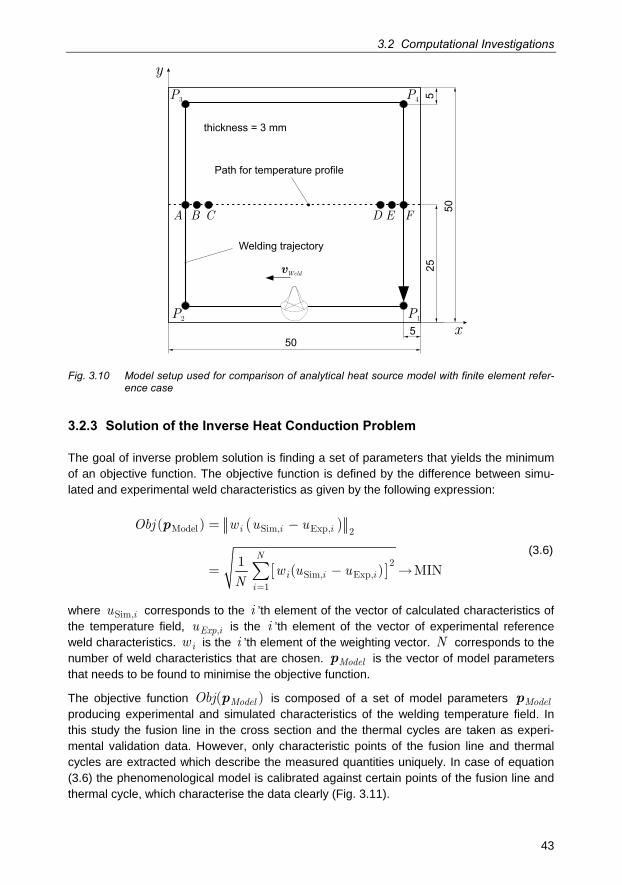
3.2 Computational Investigations
43
Path for temperature profile
y
xP1P2
P3 P4
5
50
25
50
Welding trajectory
thickness = 3 mm
vWeld
5
A B C D E F
Fig. 3.10 Model setup used for comparison of analytical heat source model with finite element refer-ence case
3.2.3 Solution of the Inverse Heat Conduction Problem
The goal of inverse problem solution is finding a set of parameters that yields the minimum of an objective function. The objective function is defined by the difference between simu-lated and experimental weld characteristics as given by the following expression:
( )
[ ]
i i i
N
i i ii
Obj w u u
w u uN
Model Sim, Exp, 2
2Sim, Exp,
1
( )
1( ) MIN
=
= -
= - å
p
(3.6)
where iuSim, corresponds to the i ’th element of the vector of calculated characteristics of the temperature field, Exp iu , is the i ’th element of the vector of experimental reference weld characteristics. iw is the i ’th element of the weighting vector. N corresponds to the number of weld characteristics that are chosen. Modelp is the vector of model parameters that needs to be found to minimise the objective function.
The objective function ModelObj( )p is composed of a set of model parameters Modelp producing experimental and simulated characteristics of the welding temperature field. In this study the fusion line in the cross section and the thermal cycles are taken as experi-mental validation data. However, only characteristic points of the fusion line and thermal cycles are extracted which describe the measured quantities uniquely. In case of equation (3.6) the phenomenological model is calibrated against certain points of the fusion line and thermal cycle, which characterise the data clearly (Fig. 3.11).
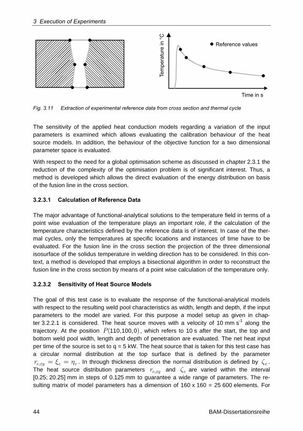
3 Execution of Experiments
44 BAM-Dissertationsreihe
Reference values
Tem
pera
ture
in °
C
Time in s
Fig. 3.11 Extraction of experimental reference data from cross section and thermal cycle
The sensitivity of the applied heat conduction models regarding a variation of the input parameters is examined which allows evaluating the calibration behaviour of the heat source models. In addition, the behaviour of the objective function for a two dimensional parameter space is evaluated.
With respect to the need for a global optimisation scheme as discussed in chapter 2.3.1 the reduction of the complexity of the optimisation problem is of significant interest. Thus, a method is developed which allows the direct evaluation of the energy distribution on basis of the fusion line in the cross section.
3.2.3.1 Calculation of Reference Data
The major advantage of functional-analytical solutions to the temperature field in terms of a point wise evaluation of the temperature plays an important role, if the calculation of the temperature characteristics defined by the reference data is of interest. In case of the ther-mal cycles, only the temperatures at specific locations and instances of time have to be evaluated. For the fusion line in the cross section the projection of the three dimensional isosurface of the solidus temperature in welding direction has to be considered. In this con-text, a method is developed that employs a bisectional algorithm in order to reconstruct the fusion line in the cross section by means of a point wise calculation of the temperature only.
3.2.3.2 Sensitivity of Heat Source Models
The goal of this test case is to evaluate the response of the functional-analytical models with respect to the resulting weld pool characteristics as width, length and depth, if the input parameters to the model are varied. For this purpose a model setup as given in chap-ter 3.2.2.1 is considered. The heat source moves with a velocity of 10 mm s-1 along the trajectory. At the position P( )110,100,0 , which refers to 10 s after the start, the top and bottom weld pool width, length and depth of penetration are evaluated. The net heat input per time of the source is set to q = 5 kW. The heat source that is taken for this test case has a circular normal distribution at the top surface that is defined by the parameter
e xy e er , x h= = . In through thickness direction the normal distribution is defined by ez . The heat source distribution parameters e xyr , and ez are varied within the interval [0.25; 20.25] mm in steps of 0.125 mm to guarantee a wide range of parameters. The re-sulting matrix of model parameters has a dimension of 160 x 160 = 25 600 elements. For
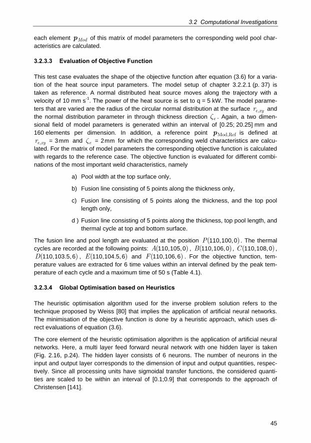
3.2 Computational Investigations
45
each element Modp of this matrix of model parameters the corresponding weld pool char-acteristics are calculated.
3.2.3.3 Evaluation of Objective Function
This test case evaluates the shape of the objective function after equation (3.6) for a varia-tion of the heat source input parameters. The model setup of chapter 3.2.2.1 (p. 37) is taken as reference. A normal distributed heat source moves along the trajectory with a velocity of 10 mm s-1. The power of the heat source is set to q = 5 kW. The model parame-ters that are varied are the radius of the circular normal distribution at the surface e xyr , and the normal distribution parameter in through thickness direction ez . Again, a two dimen-sional field of model parameters is generated within an interval of [0.25; 20.25] mm and 160 elements per dimension. In addition, a reference point Mod,Refp is defined at
e xyr , = 3mm and ez = 2mm for which the corresponding weld characteristics are calcu-lated. For the matrix of model parameters the corresponding objective function is calculated with regards to the reference case. The objective function is evaluated for different combi-nations of the most important weld characteristics, namely
a) Pool width at the top surface only,
b) Fusion line consisting of 5 points along the thickness only,
c) Fusion line consisting of 5 points along the thickness, and the top pool length only,
d ) Fusion line consisting of 5 points along the thickness, top pool length, and thermal cycle at top and bottom surface.
The fusion line and pool length are evaluated at the position P( )110,100,0 . The thermal cycles are recorded at the following points: A( )110,105,0 , B( )110,106,0 , C( )110,108,0 , D( )110,103.5,6 , E( )110,104.5,6 and F( )110,106,6 . For the objective function, tem-perature values are extracted for 6 time values within an interval defined by the peak tem-perature of each cycle and a maximum time of 50 s (Table 4.1).
3.2.3.4 Global Optimisation based on Heuristics
The heuristic optimisation algorithm used for the inverse problem solution refers to the technique proposed by Weiss [80] that implies the application of artificial neural networks. The minimisation of the objective function is done by a heuristic approach, which uses di-rect evaluations of equation (3.6).
The core element of the heuristic optimisation algorithm is the application of artificial neural networks. Here, a multi layer feed forward neural network with one hidden layer is taken (Fig. 2.16, p.24). The hidden layer consists of 6 neurons. The number of neurons in the input and output layer corresponds to the dimension of input and output quantities, respec-tively. Since all processing units have sigmoidal transfer functions, the considered quanti-ties are scaled to be within an interval of [0.1;0.9] that corresponds to the approach of Christensen [141].
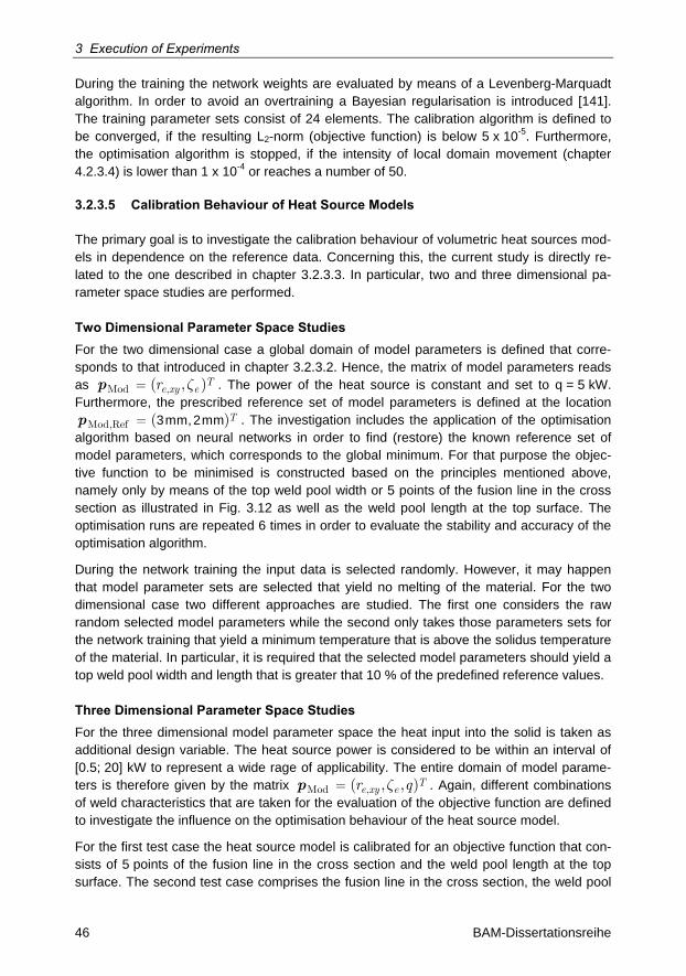
3 Execution of Experiments
46 BAM-Dissertationsreihe
During the training the network weights are evaluated by means of a Levenberg-Marquadt algorithm. In order to avoid an overtraining a Bayesian regularisation is introduced [141]. The training parameter sets consist of 24 elements. The calibration algorithm is defined to be converged, if the resulting L2-norm (objective function) is below 5 x 10⁻⁵. Furthermore, the optimisation algorithm is stopped, if the intensity of local domain movement (chapter 4.2.3.4) is lower than 1 x 10⁻⁴ or reaches a number of 50.
3.2.3.5 Calibration Behaviour of Heat Source Models
The primary goal is to investigate the calibration behaviour of volumetric heat sources mod-els in dependence on the reference data. Concerning this, the current study is directly re-lated to the one described in chapter 3.2.3.3. In particular, two and three dimensional pa-rameter space studies are performed.
Two Dimensional Parameter Space Studies For the two dimensional case a global domain of model parameters is defined that corre-sponds to that introduced in chapter 3.2.3.2. Hence, the matrix of model parameters reads as T
e xy erMod ,( , )z=p . The power of the heat source is constant and set to q = 5 kW. Furthermore, the prescribed reference set of model parameters is defined at the location
TMod,Ref ( )=p 3mm,2mm . The investigation includes the application of the optimisation
algorithm based on neural networks in order to find (restore) the known reference set of model parameters, which corresponds to the global minimum. For that purpose the objec-tive function to be minimised is constructed based on the principles mentioned above, namely only by means of the top weld pool width or 5 points of the fusion line in the cross section as illustrated in Fig. 3.12 as well as the weld pool length at the top surface. The optimisation runs are repeated 6 times in order to evaluate the stability and accuracy of the optimisation algorithm.
During the network training the input data is selected randomly. However, it may happen that model parameter sets are selected that yield no melting of the material. For the two dimensional case two different approaches are studied. The first one considers the raw random selected model parameters while the second only takes those parameters sets for the network training that yield a minimum temperature that is above the solidus temperature of the material. In particular, it is required that the selected model parameters should yield a top weld pool width and length that is greater that 10 % of the predefined reference values.
Three Dimensional Parameter Space Studies For the three dimensional model parameter space the heat input into the solid is taken as additional design variable. The heat source power is considered to be within an interval of [0.5; 20] kW to represent a wide rage of applicability. The entire domain of model parame-ters is therefore given by the matrix T
e xy er qMod ,( , , )z=p . Again, different combinations of weld characteristics that are taken for the evaluation of the objective function are defined to investigate the influence on the optimisation behaviour of the heat source model.
For the first test case the heat source model is calibrated for an objective function that con-sists of 5 points of the fusion line in the cross section and the weld pool length at the top surface. The second test case comprises the fusion line in the cross section, the weld pool
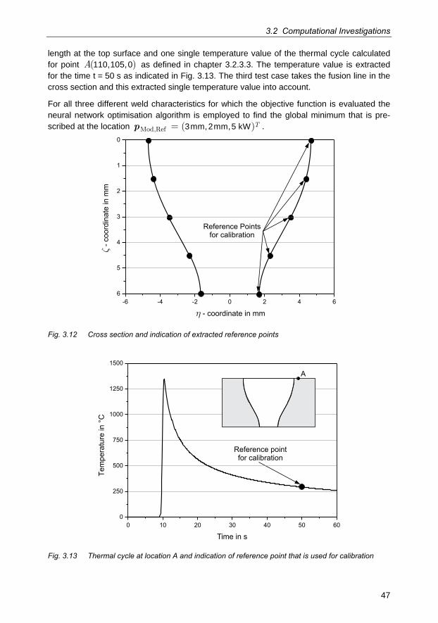
3.2 Computational Investigations
47
length at the top surface and one single temperature value of the thermal cycle calculated for point A( )110,105,0 as defined in chapter 3.2.3.3. The temperature value is extracted for the time t = 50 s as indicated in Fig. 3.13. The third test case takes the fusion line in the cross section and this extracted single temperature value into account.
For all three different weld characteristics for which the objective function is evaluated the neural network optimisation algorithm is employed to find the global minimum that is pre-scribed at the location T
Mod,Ref ( )=p 3mm,2mm,5 kW .
� - coordinate in mm
�- c
oord
inat
e in
mm
Reference Pointsfor calibration
-6 -4 -2 0 2 4 66
5
4
3
2
1
0
Fig. 3.12 Cross section and indication of extracted reference points
Reference pointfor calibration
0 10 20 30 40 50 600
250
500
750
1000
1250
1500
Tem
pera
ture
in°C
Time in s
A
Fig. 3.13 Thermal cycle at location A and indication of reference point that is used for calibration
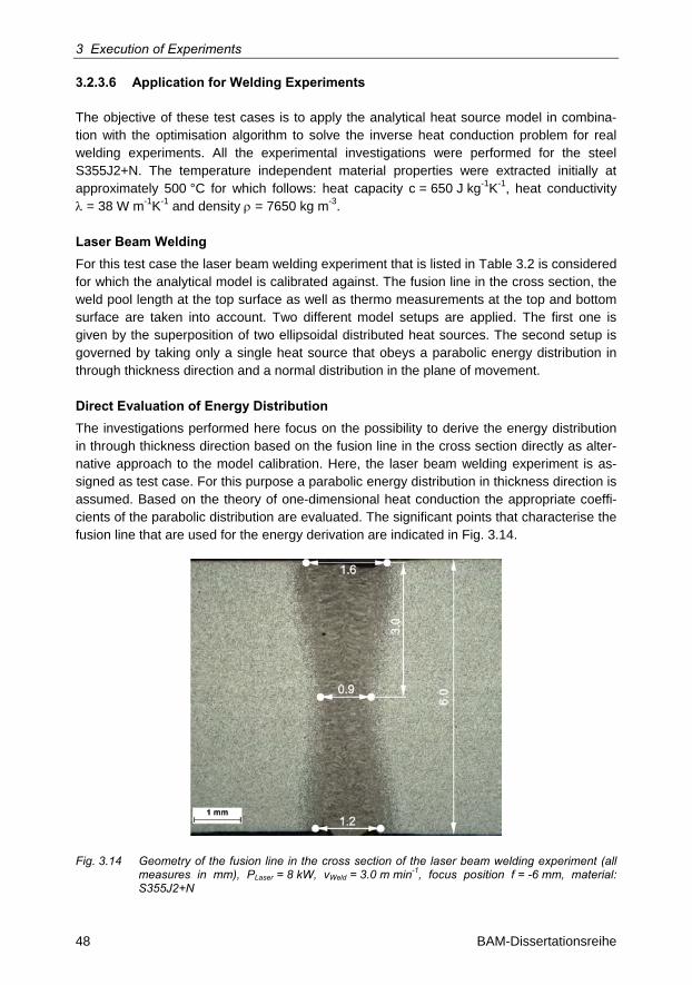
3 Execution of Experiments
48 BAM-Dissertationsreihe
3.2.3.6 Application for Welding Experiments
The objective of these test cases is to apply the analytical heat source model in combina-tion with the optimisation algorithm to solve the inverse heat conduction problem for real welding experiments. All the experimental investigations were performed for the steel S355J2+N. The temperature independent material properties were extracted initially at approximately 500 °C for which follows: heat capacity c = 650 J kg-1K-1, heat conductivity = 38 W m-1K-1 and density = 7650 kg m-3.
Laser Beam Welding For this test case the laser beam welding experiment that is listed in Table 3.2 is considered for which the analytical model is calibrated against. The fusion line in the cross section, the weld pool length at the top surface as well as thermo measurements at the top and bottom surface are taken into account. Two different model setups are applied. The first one is given by the superposition of two ellipsoidal distributed heat sources. The second setup is governed by taking only a single heat source that obeys a parabolic energy distribution in through thickness direction and a normal distribution in the plane of movement.
Direct Evaluation of Energy Distribution The investigations performed here focus on the possibility to derive the energy distribution in through thickness direction based on the fusion line in the cross section directly as alter-native approach to the model calibration. Here, the laser beam welding experiment is as-signed as test case. For this purpose a parabolic energy distribution in thickness direction is assumed. Based on the theory of one-dimensional heat conduction the appropriate coeffi-cients of the parabolic distribution are evaluated. The significant points that characterise the fusion line that are used for the energy derivation are indicated in Fig. 3.14.
Fig. 3.14 Geometry of the fusion line in the cross section of the laser beam welding experiment (all measures in mm), PLaser = 8 kW, vWeld = 3.0 m min-1, focus position f = -6 mm, material: S355J2+N

3.2 Computational Investigations
49
Laser-Gas Metal Arc Hybrid Welding The calibration of the heat source model is done for the laser-gas metal arc hybrid welding experiment that is listed in Table 3.2. The experimental reference data comprises the weld cross-section, the tailing part of the end crater as well as the thermal cycles recorded at the top and bottom surface. A superposition of a normal-parabolic and double ellipsoidal dis-tributed heat source is used to model the action of the laser beam and the arc.
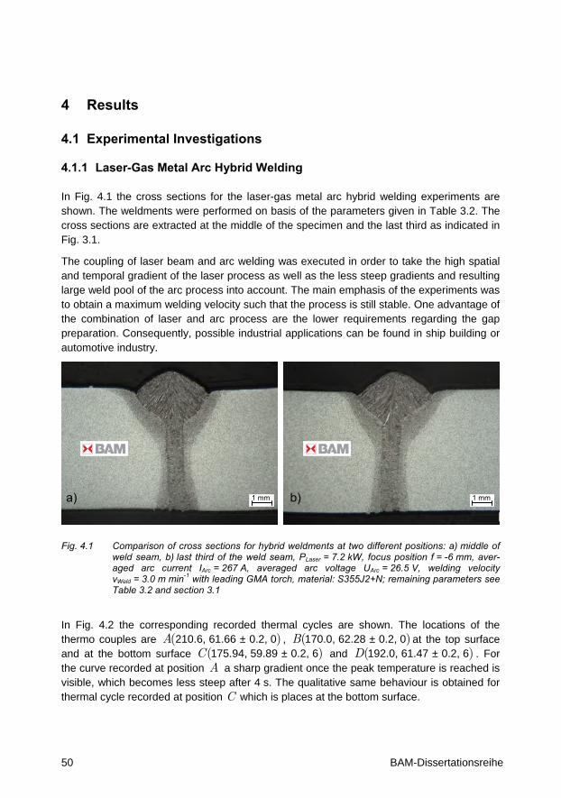
50 BAM-Dissertationsreihe
4 Results
4.1 Experimental Investigations
4.1.1 Laser-Gas Metal Arc Hybrid Welding
In Fig. 4.1 the cross sections for the laser-gas metal arc hybrid welding experiments are shown. The weldments were performed on basis of the parameters given in Table 3.2. The cross sections are extracted at the middle of the specimen and the last third as indicated in Fig. 3.1.
The coupling of laser beam and arc welding was executed in order to take the high spatial and temporal gradient of the laser process as well as the less steep gradients and resulting large weld pool of the arc process into account. The main emphasis of the experiments was to obtain a maximum welding velocity such that the process is still stable. One advantage of the combination of laser and arc process are the lower requirements regarding the gap preparation. Consequently, possible industrial applications can be found in ship building or automotive industry.
a) b)1 mm
1 mm 1 mm
Fig. 4.1 Comparison of cross sections for hybrid weldments at two different positions: a) middle of weld seam, b) last third of the weld seam, PLaser = 7.2 kW, focus position f = -6 mm, aver-aged arc current IArc = 267 A, averaged arc voltage UArc = 26.5 V, welding velocity vWeld = 3.0 m min-1 with leading GMA torch, material: S355J2+N; remaining parameters see Table 3.2 and section 3.1
In Fig. 4.2 the corresponding recorded thermal cycles are shown. The locations of the thermo couples are A( )210.6, 61.66 ± 0.2, 0 , B( )170.0, 62.28 ± 0.2, 0 at the top surface and at the bottom surface C( )175.94, 59.89 ± 0.2, 6 and D( )192.0, 61.47 ± 0.2, 6 . For the curve recorded at position A a sharp gradient once the peak temperature is reached is visible, which becomes less steep after 4 s. The qualitative same behaviour is obtained for thermal cycle recorded at position C which is places at the bottom surface.
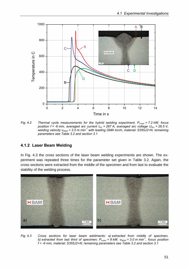
4.1 Experimental Investigations
51
0 2 4 6 8 10 12 140
200
400
600
800
1000
Tem
pera
ture
inC
Time in s
A
B
C
D
D
BA
C
Fig. 4.2 Thermal cycle measurements for the hybrid welding experiment, PLaser = 7.2 kW, focus position f = -6 mm, averaged arc current IArc = 267 A, averaged arc voltage UArc = 26.5 V, welding velocity vWeld = 3.0 m min-1 with leading GMA torch, material: S355J2+N; remaining parameters see Table 3.2 and section 3.1
4.1.2 Laser Beam Welding
In Fig. 4.3 the cross sections of the laser beam welding experiments are shown. The ex-periment was repeated three times for the parameter set given in Table 3.2. Again, the cross sections were extracted from the middle of the specimen and from last to evaluate the stability of the welding process.
a) b) 1 mm1 mm
Fig. 4.3 Cross sections for laser beam weldments: a) extracted from middle of specimen, b) extracted from last third of specimen; PLaser = 8 kW, vWeld = 3.0 m min-1, focus position f = -6 mm, material: S355J2+N; remaining parameters see Table 3.2 and section 3.1
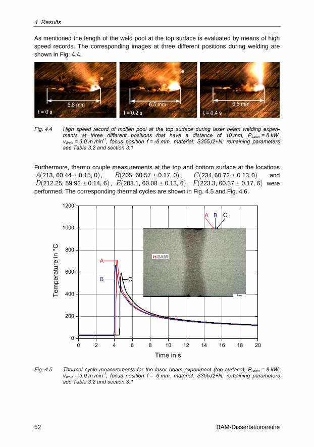
4 Results
52 BAM-Dissertationsreihe
As mentioned the length of the weld pool at the top surface is evaluated by means of high speed records. The corresponding images at three different positions during welding are shown in Fig. 4.4.
Fig. 4.4 High speed record of molten pool at the top surface during laser beam welding experi-ments at three different positions that have a distance of 10 mm, PLaser = 8 kW, vWeld = 3.0 m min-1, focus position f = -6 mm, material: S355J2+N; remaining parameters see Table 3.2 and section 3.1
Furthermore, thermo couple measurements at the top and bottom surface at the locations A( )213, 60.44 ± 0.15, 0 , B( )205, 60.57 ± 0.17, 0 , C( )234, 60.72 ± 0.13, 0 and D( )212.25, 59.92 ± 0.14, 6 , E( )203.1, 60.08 ± 0.13, 6 , F( )223.3, 60.37 ± 0.17, 6 were performed. The corresponding thermal cycles are shown in Fig. 4.5 and Fig. 4.6.
CB
A
0 2 4 6 8 10 12 14 16 18 200
200
400
600
800
1000
1200
Time in s
Tem
pera
ture
in°C
CBA
Fig. 4.5 Thermal cycle measurements for the laser beam experiment (top surface), PLaser = 8 kW, vWeld = 3.0 m min-1, focus position f = -6 mm, material: S355J2+N; remaining parameters see Table 3.2 and section 3.1
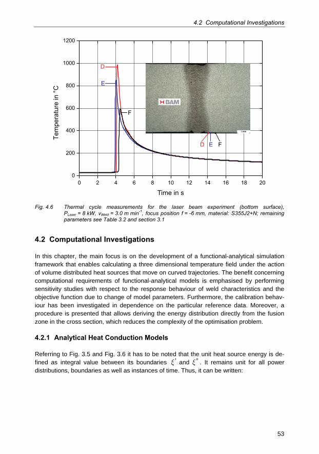
4.2 Computational Investigations
53
0 2 4 6 8 10 12 14 16 18 200
200
400
600
800
1000
1200
Tem
pera
ture
in°C
Time in s
F
E
D
ED F
Fig. 4.6 Thermal cycle measurements for the laser beam experiment (bottom surface), PLaser = 8 kW, vWeld = 3.0 m min-1, focus position f = -6 mm, material: S355J2+N; remaining parameters see Table 3.2 and section 3.1
4.2 Computational Investigations
In this chapter, the main focus is on the development of a functional-analytical simulation framework that enables calculating a three dimensional temperature field under the action of volume distributed heat sources that move on curved trajectories. The benefit concerning computational requirements of functional-analytical models is emphasised by performing sensitivity studies with respect to the response behaviour of weld characteristics and the objective function due to change of model parameters. Furthermore, the calibration behav-iour has been investigated in dependence on the particular reference data. Moreover, a procedure is presented that allows deriving the energy distribution directly from the fusion zone in the cross section, which reduces the complexity of the optimisation problem.
4.2.1 Analytical Heat Conduction Models
Referring to Fig. 3.5 and Fig. 3.6 it has to be noted that the unit heat source energy is de-fined as integral value between its boundaries 'x and ''x . It remains unit for all power distributions, boundaries as well as instances of time. Thus, it can be written:
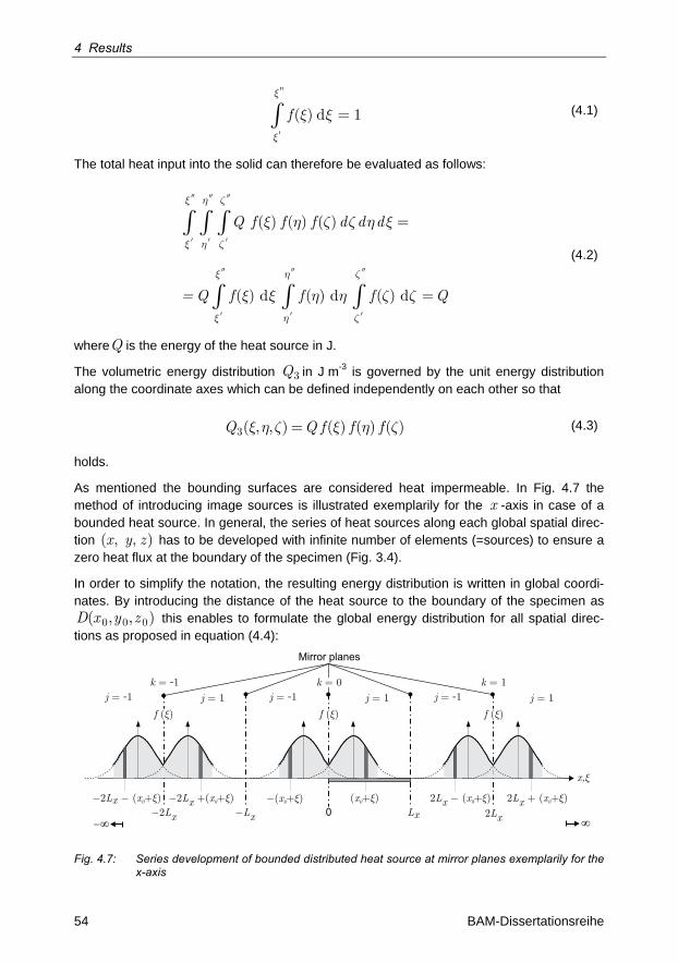
4 Results
54 BAM-Dissertationsreihe
f
''
'
( ) d 1
x
x
x x =ò (4.1)
The total heat input into the solid can therefore be evaluated as follows:
Q f f f d d d
= Q f f f Q
( ) ( ) ( )
( ) d ( ) d ( ) d
x h z
x h z
x h z
x h z
x h z z h x
x x h h z z
¢ ¢ ¢
¢ ¢ ¢
=
=
ò ò ò
ò ò ò
(4.2)
whereQ is the energy of the heat source in J.
The volumetric energy distribution Q3 in J m-3 is governed by the unit energy distribution along the coordinate axes which can be defined independently on each other so that
Q Q f f f3( , , ) ( ) ( ) ( )x h z x h z= (4.3)
holds.
As mentioned the bounding surfaces are considered heat impermeable. In Fig. 4.7 the method of introducing image sources is illustrated exemplarily for the x -axis in case of a bounded heat source. In general, the series of heat sources along each global spatial direc-tion x y z( , , ) has to be developed with infinite number of elements (=sources) to ensure a zero heat flux at the boundary of the specimen (Fig. 3.4).
In order to simplify the notation, the resulting energy distribution is written in global coordi-nates. By introducing the distance of the heat source to the boundary of the specimen as D x y z0 0 0( , , ) this enables to formulate the global energy distribution for all spatial direc-tions as proposed in equation (4.4):
Lx Lx0( + )x0 �
j = 1j = -1
k = 0
2Lx
2 +( + )x0 �Lx 2 ( + )L xx 0 �
k = -1
2Lx
2 + ( + )x0 �Lx2 ( + )x 0 �Lx
k = 1
�� �
x,�
Mirror planes
( + )x0 �
f ( )�f ( )� f ( )�
j = 1j = -1 j = 1j = -1
Fig. 4.7: Series development of bounded distributed heat source at mirror planes exemplarily for the x-axis
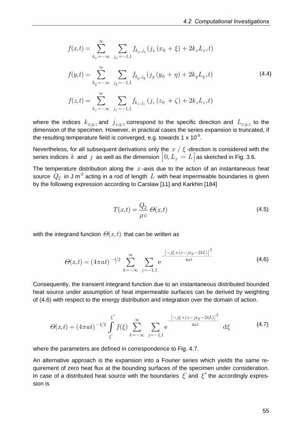
4.2 Computational Investigations
55
x x
x x
y y
y y
z z
z z
k ,j x x xk j
k ,j y y yk j
k ,j z z zk j
f x,t f j x k L ,t
f y,t f j y k L ,t
f z,t f j z k L ,t
01,1
01,1
01,1
( ) ( ( ) + 2 )
( ) ( ( + ) + 2 )
( ) ( ( + ) + 2 )
x
h
z
¥
=-¥ =-
¥
=-¥ =-
¥
=-¥ =-
= +
=
=
å å
å å
å å
(4.4)
where the indices x,y,zk and x,y,zj correspond to the specific direction and x y zL , , to the dimension of the specimen. However, in practical cases the series expansion is truncated, if the resulting temperature field is converged, e.g. towards 1 x 10⁻⁵.
Nevertheless, for all subsequent derivations only the x / x -direction is considered with the series indices k and j as well as the dimension xL L0,é ù=ë û as sketched in Fig. 3.6.
The temperature distribution along the x -axis due to the action of an instantaneous heat source Q2 in J m-2 acting in a rod of length L with heat impermeable boundaries is given by the following expression according to Carslaw [11] and Karkhin [184]
QT x,t = x,t
c2( ) ( )Q
r (4.5)
with the integrand function x t( , )Q that can be written as
[ ]0j x jx kL
at
k j
x,t = at
2( 2 )
1 2 4
1,1
( ) (4 ) e
x
Q p- + - -¥ -
-
=-¥ =-å å (4.6)
Consequently, the transient integrand function due to an instantaneous distributed bounded heat source under assumption of heat impermeable surfaces can be derived by weighting of (4.6) with respect to the energy distribution and integration over the domain of action.
[ ]0j x jx kL
at
k j
x,t = at f
2''
'
( 2 )
1 2 4
1,1
( ) (4 ) ( ) e d
x x
x
Q p x x- + - -¥ -
-
=-¥ =-å åò (4.7)
where the parameters are defined in correspondence to Fig. 4.7.
An alternative approach is the expansion into a Fourier series which yields the same re-quirement of zero heat flux at the bounding surfaces of the specimen under consideration. In case of a distributed heat source with the boundaries 'x and ''x the accordingly expres-sion is
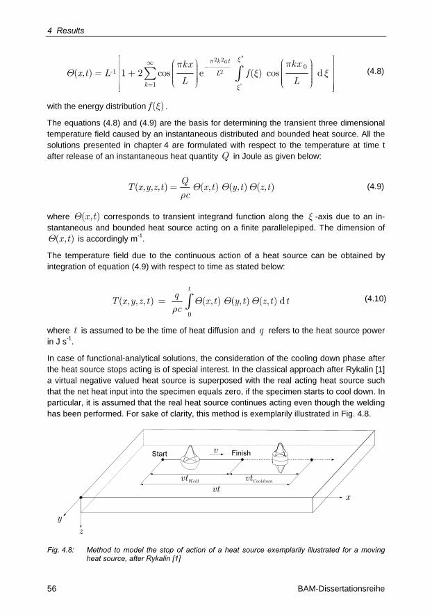
4 Results
56 BAM-Dissertationsreihe
k at
L
k=
kxkxx,t = L f
L L
''2 2
2
'
0-1
1
( ) 1 + 2 cos e ( ) cos d
xp
x
ppQ x x
¥-
é ùæ öæ öê ú÷÷ çç ÷÷ ççê ú÷÷ çç ÷÷ çê ú÷ç ÷çè ø è øê úë ûå ò (4.8)
with the energy distribution f ( )x .
The equations (4.8) and (4.9) are the basis for determining the transient three dimensional temperature field caused by an instantaneous distributed and bounded heat source. All the solutions presented in chapter 4 are formulated with respect to the temperature at time t after release of an instantaneous heat quantity Q in Joule as given below:
QT x,y,z,t x,t y,t z,t
c( ) ( ) ( ) ( )Q Q Q
r= (4.9)
where x,t( )Q corresponds to transient integrand function along the x -axis due to an in-stantaneous and bounded heat source acting on a finite parallelepiped. The dimension of
x,t( )Q is accordingly m-1.
The temperature field due to the continuous action of a heat source can be obtained by integration of equation (4.9) with respect to time as stated below:
tq
T x y z t x t y t z t tc
0
( , , , ) = ( , ) ( , ) ( , ) dQ Q Qr ò (4.10)
where t is assumed to be the time of heat diffusion and q refers to the heat source power in J s-1.
In case of functional-analytical solutions, the consideration of the cooling down phase after the heat source stops acting is of special interest. In the classical approach after Rykalin [1] a virtual negative valued heat source is superposed with the real acting heat source such that the net heat input into the specimen equals zero, if the specimen starts to cool down. In particular, it is assumed that the real heat source continues acting even though the welding has been performed. For sake of clarity, this method is exemplarily illustrated in Fig. 4.8.
Start Finish
vtWeld vtCooldown
vtx
y
z
v
Fig. 4.8: Method to model the stop of action of a heat source exemplarily illustrated for a moving heat source, after Rykalin [1]
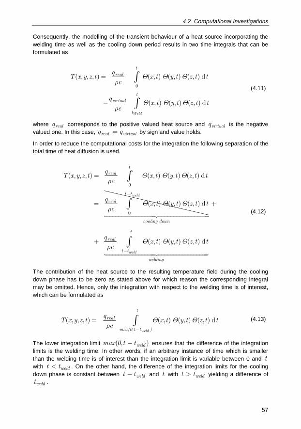
4.2 Computational Investigations
57
Consequently, the modelling of the transient behaviour of a heat source incorporating the welding time as well as the cooling down period results in two time integrals that can be formulated as
Weld
treal
tvirtual
t
qT x y z t x t y t z t t
c
qx t y t z t t
c
0
( , , , ) = ( , ) ( , ) ( , ) d
( , ) ( , ) ( , ) d
Q Q Qr
Q Q Qr
-
ò
ò
(4.11)
where realq corresponds to the positive valued heat source and virtualq is the negative valued one. In this case, real virtualq q= by sign and value holds.
In order to reduce the computational costs for the integration the following separation of the total time of heat diffusion is used.
weld
treal
t t
real
qT x y z t x t y t z t t
c
qx t y t z t t
c
0
0
( , , , ) = ( , ) ( , ) ( , ) d
( , ) ( , ) ( , ) d
Q Q Qr
Q Q Qr
-
=
ò
ò
weld
cooling down
t
real
t t
welding
qx t y t z t t
c( , ) ( , ) ( , ) dQ Q Q
r-
+
+ ò
(4.12)
The contribution of the heat source to the resulting temperature field during the cooling down phase has to be zero as stated above for which reason the corresponding integral may be omitted. Hence, only the integration with respect to the welding time is of interest, which can be formulated as
weld
t
real
max(0,t t )
qT x y z t x t y t z t t
c( , , , ) = ( , ) ( , ) ( , ) dQ Q Q
r-ò (4.13)
The lower integration limit weldmax 0,t t( )- ensures that the difference of the integration limits is the welding time. In other words, if an arbitrary instance of time which is smaller than the welding time is of interest than the integration limit is variable between 0 and t with weldt t< . On the other hand, the difference of the integration limits for the cooling down phase is constant between weldt t- and t with weldt t> yielding a difference of
weldt .
4 Results
58 BAM-Dissertationsreihe
4.2.1.1 Normal Distribution
The normal energy distribution has to meet equation (4.1). Applying the formulae 1.3.3.1 of the tables of integrals after Prudnikov [185] yields the following expressions
eee e
e ee e e e
f
'' '' 2
' '
1'' '
1'' ' '' '
2( ) d e d
2
2
x x
x x
xxx x
x x x F F xx xp
x x p x xx F F x F F
x x x xp
æ ö- ÷ç- ÷ç ÷÷çè ø
-
ì é æ ö æ öù üï ïï ï÷ ÷ç ç= ê - ú÷ ÷í ýç ç÷ ÷ç çï ïê è ø è øúï ïî ë û þ
ì é æ ö æ öù ü é æ ö æ öùï ïï ï÷ ÷ ÷ ÷ç ç ç ç= ê - ú ê -÷ ÷ ÷ ÷í ýç ç ç ç÷ ÷ ÷ ÷ç ç ç çï ïê è ø è øú ê è ø è øï ïî ë û þ ë
ò ò
1ú =úû
(4.14)
verifying that the unity is conserved.
The one dimensional integrand function for a normal distributed heat source can be derived with reference to the parameter system illustrated in Fig. 3.6 and Fig. 4.7. By insertion of equation (3.1) at page 36 into equation (4.7) the solution for the image source method can be found as:
( )
[ ]0
eee e
-j x jx kL
at
k j
x,t at
'' 2
'
2
1'' '1 2
( 2 )
4
1,1
2( ) 4 e
e d
x
x
x
xxx x
Q p x F Fx xp
x
æ ö- ÷ç- ÷ç- ÷÷çè ø
æ ö÷ç + - - ÷ç ÷¥ -ç ÷ç ÷ç ÷÷çè ø
=-¥ =-
ì é æ ö æ öù üï ïï ï÷ ÷ç ç= ê - ú *÷ ÷í ýç ç÷ ÷ç çï ïê è ø è øúï ïî ë û þ
*
ò
å å
(4.15)
After performing the integration with respect to the independent variable x and using the integral tables of Prudnikov [185] chapter 1.3.3.17 the integral can be solved directly. The resulting functional-analytical expression for the integrand function along the x -axis due to an instantaneous normal distributed heat source bounded by 'x and ''x can be written as:
ξ
ξ
0
e
ee e
( x jx kL)
at
k j
x,t at
F F
2
2
1'' '
2
2
4 '' '
1,1
( ) (4 )
e ( ) ( )
x xQ p F F
x x
x x
-
- -¥ -
+
=-¥ =-
ì é æ ö æ öù üï ïï ï÷ ÷ç ç= + ê - ú *÷ ÷í ýç ç÷ ÷ç çï ïê è ø è øúï ïî ë û þ
é ù* * -ë ûå å
(4.16)
In order to simplify the expression the function F u( ) was introduced which reads as
( )0 ee
e e
j x jx kLuF u =
a t a t a t
2
2
( 2 )( ) 1
4 4 4 +
xxF
x x
æ ö- - ÷ç ÷ç + - ÷ç ÷ç ÷çè ø (4.17)
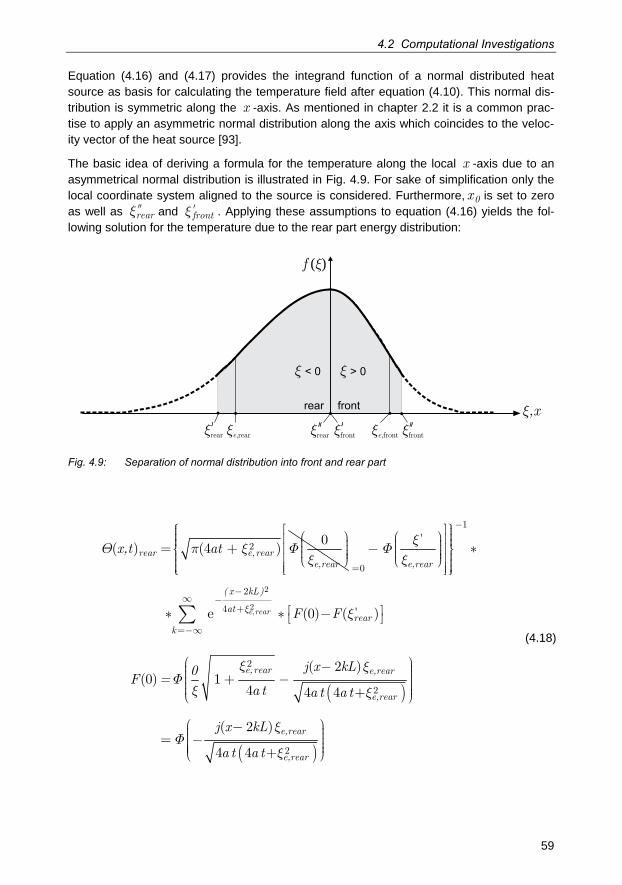
4.2 Computational Investigations
59
Equation (4.16) and (4.17) provides the integrand function of a normal distributed heat source as basis for calculating the temperature field after equation (4.10). This normal dis-tribution is symmetric along the x -axis. As mentioned in chapter 2.2 it is a common prac-tise to apply an asymmetric normal distribution along the axis which coincides to the veloc-ity vector of the heat source [93].
The basic idea of deriving a formula for the temperature along the local x -axis due to an asymmetrical normal distribution is illustrated in Fig. 4.9. For sake of simplification only the local coordinate system aligned to the source is considered. Furthermore, 0x is set to zero as well as rearx and frontx ¢ . Applying these assumptions to equation (4.16) yields the fol-lowing solution for the temperature due to the rear part energy distribution:
f ( )�
��x
�rear
/�rear
//
� < 0 � > 0
frontrear
�front
/�front
//�e,rear �e,front
Fig. 4.9: Separation of normal distribution into front and rear part
rear e,reare,rear
x,t at 20
( ) (4 )Q p x Fx
æ ö÷ç= + ÷ç ÷ç ÷è ø
( )
e,rear
e,rear
( x kL)
atrear
k
e,rear e,rear
e,rear
e,rear
e,
F F
j x kL0F =
a t a t a t
j x kL
a t a t
2
2
1'
0
2
4 + '
2
2
e (0) ( )
( 2 )(0) 1
4 4 4 +
( 2 )
4 4 +
x
xF
x
x
x xF
x x
xF
x
-
=
-¥ -
=-¥
ì é ù üï ïæ öï ïê úï ï÷ç- ÷ *ê úí ýç ÷ç ÷ï ïê úè øï ïê úï ïî ë û þ
é ù* * -ë û
æ ö- ÷ç ÷ç ÷+ -ç ÷ç ÷÷çè ø
-= -
å
( )rear2
æ ö÷ç ÷ç ÷ç ÷ç ÷çè ø
(4.18)
4 Results
60 BAM-Dissertationsreihe
The same approach can be applied for the front part of the energy distribution. Setting
frontx ¢ and 0x to zero this allows writing
frontfront e, front
e, front e, front
x,t at''
2 0( ) (4 )
xQ p x F F
x x
æ ö æ ö÷ ÷ç ç÷ ÷ç ç= + -÷ ÷ç ç÷ ÷ç ç÷ ÷ç çè ø è ø
( )
( )
ξe front
( x kL)
atfront
k
e, front e, front
e, front
e, front
e, front
F F
j x kL0F =
a t a t a t+
j x- kL
a t a t+
2
2,
1
0
2
4 ''
2
2
2
e ( ) (0)
( 2 )(0) 1
4 4 4
( 2 )
4 4
x
x xF
x x
xF
x
-
=
-¥ -
+
=-¥
ì é ù üï ïï ïê úï ïï ïê ú *í ýê úï ïï ïê úï ïï ïî ë û þ
é ù* * -ë û
æ ö- ÷ç ÷ç ÷+ -ç ÷ç ÷ç ÷çè ø
æçç= -è
å
ö÷÷÷ç ÷ç ÷ç ÷ç ø
(4.19)
Equation (4.18) and (4.19) enable to evaluate the resulting integrand function along the x -axis due to an instantaneous asymmetrical normal distributed heat source as
rear frontx,t x,t x,t( ) ( ) ( )Q Q Q= + (4.20)
However, the net heat input has also to be separated into a front and a rear part. In general, the equation rear frontQ Q Q= + holds. The energy input of the heat source for the front part and the rear part can be formulated as [90]:
fronte,front
e,front
frontfront rear
e,front e,reare,front e,rear
reare,rear
e,rear
rearfront
e,fronte,front
Q Q
Q
''
'' '
'
''
xx F
x
x xx F x Fx x
xx F
x
xx F x
x
æ ö÷ç ÷ç ÷ç ÷ç ÷è ø=
æ ö æ ö÷ ÷ç ç÷ ÷ç ç-÷ ÷ç ç÷ ÷ç ç÷ ÷è ø è ø
æ ö÷ç ÷ç- ÷ç ÷ç ÷è ø=
æ ö÷ç ÷ç -÷ç ÷ç ÷è ørear
e,reare,rear
Q'x
Fx
æ ö÷ç ÷ç ÷ç ÷ç ÷è ø
(4.21)
4.2 Computational Investigations
61
As mentioned above the development of a FOURIER series of a normal distributed instanta-neous heat source which is bounded by 'x as well as ''x and acting in a rod of lengthL can be done by inserting formula (3.1) into (4.8). The integral can be solved directly by applying the substitution 1.5.49 of Prudnikov [185] which ends with the following expression:
( ) ( )[ ]e
e e
kat
L
k
x tL
k xF F
L
2 2 2
2
-1'' '
4 '' '
1
1 2( , ) 1
* cos ep x
x xQ F F
x xp
px x
æ ö¥ ÷ç ÷- +ç ÷ç ÷çè ø
=
ìï é æ ö æ öùïï ÷ ÷ç ç= + * ê - ú÷ ÷í ç ç÷ ÷ç çï ê è ø è øúë ûïïî
üïæ ö ïï÷ç -÷ ýç ÷ç ïè ø ïïþå
(4.22)
In this case the function F u( ) has the subsequent structure:
0 e
e
0 e
e
k x kuF u i
L L
k x kui
L L
( ) cos Re2
sin Im2
p pxF
x
p pxF
x
æ ö é æ öù÷ ÷ç çê ú÷ ÷ç ç= - -÷ ÷ç çê ú÷ ÷÷ ÷ç çè ø è øê úë ûæ ö é æ öù÷ ÷ç çê ú÷ ÷ç ç- -÷ ÷ç çê ú÷ ÷÷ ÷ç çè ø è øê úë û
(4.23)
where
w
w h h w r is i2
0
2( ) exp(- )d -1F
p= = + =ò and with (4.24)
In this context the variable w corresponds to the complex number with the real part r and the imaginary part s . The main aspect that has to be mentioned here is that equation (4.23) is complex due to the complex error function w( )F . It is convenient to write the complex error function in the following way [186]
h
w K r s i M r s
i edh
w h
2-
-
( ) ( , ) ( , )
-
F
p
¥
¥
= +
= ò (4.25)
where K r s( , ) is referred to as VOIGT-function and M r s( , ) as LORENTZ-function. A common approach is to apply rational approximation algorithms in order to evaluate equation (4.25). Schreier [186] gives an overview of different algorithms which focus on the approximation of the VOIGT-function, i.e. the real part of the complex error function. Weideman [187] presents algorithms for the calculation of the complex error function. These are based on rational expansions as they are listed in Abramowitz [188].
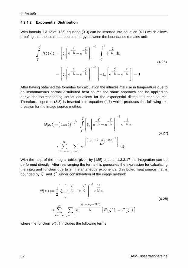
4 Results
62 BAM-Dissertationsreihe
4.2.1.2 Exponential Distribution
With formula 1.3.13 of [185] equation (3.3) can be inserted into equation (4.1) which allows proofing that the total heat source energy between the boundaries remains unit:
e e e
e e e e
e
e e
f
'' ''' ''
' '
' '' '' '
1
1
( ) d e e e d
e e e e 1
x xx x xx x x
x x
x x x xx x x x
x x x x
x x
-- - -
-- - - -
é æ ö ù÷çê ú÷ç= - ÷çê ú÷ç ÷÷çê úè øë û
é æ ö ù é æ öù÷ ÷ç çê ú ê ú÷ ÷ç ç= - - - =÷ ÷ç çê ú ê ú÷ ÷ç ç÷ ÷÷ ÷ç çê ú ê úè ø è øë û ë û
ò ò (4.26)
After having obtained the formulae for calculation the infinitesimal rise in temperature due to an instantaneous normal distributed heat source the same approach can be applied to derive the corresponding set of equations for the exponential distributed heat source. Therefore, equation (3.3) is inserted into equation (4.7) which produces the following ex-pression for the image source method:
( )
[ ]
e e e
0
e
j x jx kL
at
k j
x,t at
'' ' ''
'
2
1
1 2
( 2 )
4
1,1
( ) 4 e e e
e d
x x x xx x x
x
x
Q p x
x
-
- - --
æ ö÷ç - + - - ÷ç ÷¥ -ç ÷ç ÷ç ÷÷çè ø
=-¥ =-
é æ öù÷çê ú÷ç= - *÷çê ú÷ç ÷÷çê úè øë û
*
ò
å å
(4.27)
With the help of the integral tables given by [185] chapter 1.3.3.17 the integration can be performed directly. After rearranging the terms this generates the expression for calculating the integrand function due to an instantaneous exponential distributed heat source that is bounded by 'x and ''x under consideration of the image method:
( ) ( )
e e e
0
e
a t
e
j x jx kL
k j
x t
F F
' ''
2
-1
( 2 )
'' '
1,1
1( , ) e e e
2
e
x xx x x
x
Q x
x x
- -
- -¥ -
=-¥ =-
é æ öù÷çê ú÷ç= - *÷çê ú÷ç ÷÷çê úè øë û
é ù* -ë ûå å
(4.28)
where the function F u( ) includes the following terms
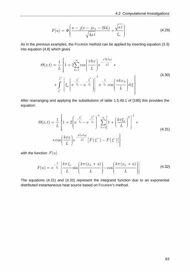
4.2 Computational Investigations
63
0
e
a tu j x jx kLF u
a t
( 2 )( )
4F
x
æ ö- - - ÷ç ÷ç= + ÷ç ÷ç ÷çè ø (4.29)
As in the previous examples, the FOURIER method can be applied by inserting equation (3.3) into equation (4.8) which gives
e e e
k at
L
k=
e
kxx,t
L L
kx
L
2 2
2
'' ' ''
'
1
-1
0
1( ) 1 + 2 cos e
e e e cos d
p
x x x xx x x
x
pQ
px x
¥-
- - -
ìï æ öï ÷çï ÷ç= *í ÷ç ÷ï ÷çè øïïîüïïé æ öù æ ö ï÷ ÷ç çê ú ï÷ ÷ç ç* - ÷ ý÷çê ú ç÷ ÷ç ïç÷ ÷ç÷çê ú è ø ïè øë û ïïþ
å
ò
(4.30)
After rearranging and applying the substitutions of table 1.5.49.1 of [185] this provides the equation:
( ) ( )[ ]
e ee
k
k at
L
kx t
L L
k xF F
L
' ''
2 2
2
-1 -12
1
'' '
1( , ) 1 2 e e 1
cos e
x xx x
p
pxQ
px x
¥- -
=
-
ìï æ ö é ùï æ ö÷çïï ê ú÷ ÷çç= + - + *÷ ÷í çç ê ú÷ ÷ççï è ø÷÷ç ê úï è ø ë ûïïîüïæ ö ï÷ç* -÷ ýç ÷ç ïè ø ïþ
å (4.31)
with the function F u( )
e
ue 0 0k k x u k x u
F uL L L
( + ) ( + )( ) e sin cosx
p x p p- é æ ö æ öù÷ ÷ç çê ú÷ ÷ç ç= -÷ ÷ç çê ú÷ ÷÷ ÷ç çè ø è øê úë û (4.32)
The equations (4.31) and (4.32) represent the integrand function due to an exponential distributed instantaneous heat source based on FOURIER’S method.
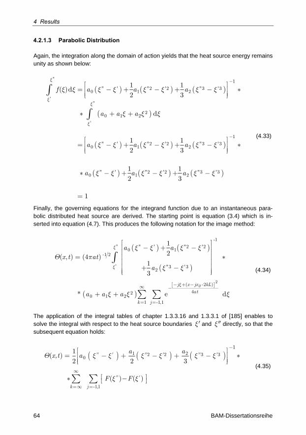
4 Results
64 BAM-Dissertationsreihe
4.2.1.3 Parabolic Distribution
Again, the integration along the domain of action yields that the heat source energy remains unity as shown below:
( ) ( ) ( )
( )
( ) ( ) ( )
( ) ( ) ( )
f a a a
a a a
a a a
a a a
''
'''
'
1
'' ' '' 2 '2 '' 3 ' 30 1 2
20 1 2
1
'' ' '' 2 '2 '' 3 ' 30 1 2
'' ' '' 2 '2 '' 3 ' 30 1 2
1 1( )d
2 3
d
1 1
2 3
1 1
2 3
1
x
xx
x
x x x x x x x x
x x x
x x x x x x
x x x x x x
-
-
é ù= ê - + - + - ú *
ê úë û
* + +
é ù= ê - + - + - ú *
ê úë û
* - + - + -
=
ò
ò
(4.33)
Finally, the governing equations for the integrand function due to an instantaneous para-bolic distributed heat source are derived. The starting point is equation (3.4) which is in-serted into equation (4.7). This produces the following notation for the image method:
( ) ( )
( )
( )[ ]0
-
j x jx kL
at
k j
a ax t at
a
a a a
''
'
2
1
'' ' '' 2 '20 1
-1 2
'' 3 ' 32
( -2 )
420 1 2
1 -1,1
1
2( , ) (4 )1
3
* e d
x
x
x
x x x xQ p
x x
x x x- + -¥ -
= =
é ùê ú- + -ê ú
= *ê úê úê ú+ -ê úë û
+ +
ò
å å
(4.34)
The application of the integral tables of chapter 1.3.3.16 and 1.3.3.1 of [185] enables to solve the integral with respect to the heat source boundaries x¢ and x directly, so that the subsequent equation holds:
( ) ( ) ( )'' ' '' ' '' '
'' '
k j
a ax,t a
F F
1 22 2 3 30
-1,1
11
( )2 2 3
( ) ( )
Q x x x x x x
x x¥
=¥ =
-é ù= ê - + - + - ú *
ê úë û
é ù* -ë ûå å (4.35)

4.2 Computational Investigations
65
where the function F u( ) includes the following terms:
( )[ ]
( )
{
u j x jx kL
a t
a tF u a a u j x jx kL a j x jx kL
a a j x jx kL a a t a x jx kL
u j x jx kL
a t
20
1 2 0 2 0
( 2 )
4
20 1 0 2 2 0
0
4( ) ( 2 ) 2 ( 2 )
e
( 2 ) 2 ( 2 )
( 2 )
4
p
F
- - --
= - - - - - - - - *
* +
é ù+ + - - + + - -ë ûæ öüï- - - ÷ç ï÷ç* ý÷ç ÷ïç ÷çè øïþ
(4.36)
The same approach can be performed in order to develop the solution with basis on the FOURIER’S method. Therefore, equation (3.4) is inserted into equation (4.8). This allows writing the equation for the integrand function due to a parabolic distributed instantaneous heat source under consideration of the heat source boundaries x ¢ and x as given in the below mentioned formula:
( ) ( ) ( )
( )
k at
L
k=
kxx,t
L L
a a a
kxa a a d
L
2 2
2
''
'
1
1
'' ' '' 2 '2 '' 3 ' 30 1 2
02
0 1 2
1( ) 1 + 2 cos e
1 1*
2 3
* cos
p
x
x
pQ
x x x x x x
px x x
¥-
-
ìï æ öï ÷çï ÷ç= *í ÷ç ÷ï ÷çè øïïî
é ù* ê - + - + - ú
ê úë û
æ ö üï÷ç ï÷ç+ + ý÷ç ÷ ïç ÷çè ø ïþ
å
ò (4.37)
The application of the integral substitution presented by [185] in chapter 1.5.52.6 and 1.5.51.7 allows to provide a closed form solution of equation (4.37):
( ) ( ) ( )
( ) ( )k
a ax t a
L
k x k a tLF F
k L L
11 2'' ' '' 2 '2 '' 3 ' 3
0
2 2'' '
21
1( , ) 1 2 *
2 3
* cos exp
Q x x x x x x
p px x
p
-
¥
=
ìï é ùïï= + ê - + - + - úíï ê úë ûïïîæ ö æ ö ü- ï÷ ÷ç ç ï÷ ÷ é ùç ç - ý÷ ÷ç ç ë û÷ ÷ ï÷ ÷ç çè ø è ø ïþ
å (4.38)
where the functionF u( ) stands for
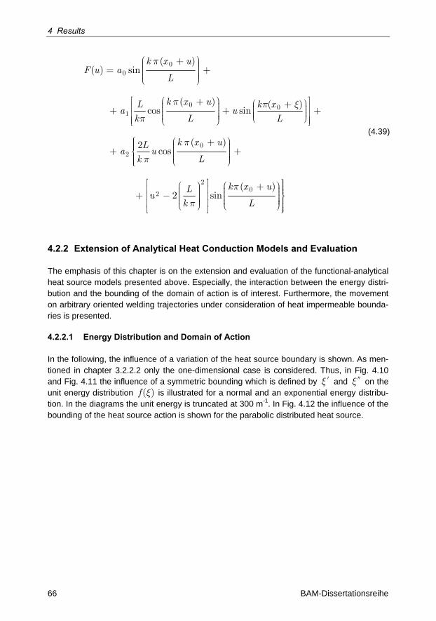
4 Results
66 BAM-Dissertationsreihe
k x uF u a
L
k x u k xLa u
k L L
k x uLa u
k L
k x uLu
k L
00
0 01
02
20
2
( )( ) sin
( ) ( )cos sin
( )2cos
( )2 sin
p
p p xp
p
p
p
p
æ ö+ ÷ç ÷ç= +÷ç ÷÷çè ø
é æ ö ù+ æ ö+÷çê ú÷ç÷ç+ + +÷÷ ççê ú÷ç÷ è ø÷çè øê úë û
ì æ ö+ï ÷çï ÷ç+ +í ÷ç ÷ï ÷çè øïî
é ù üïæ ö æ ö+ê ú÷ ÷ç ç÷ ÷ç ç+ - ýê ú÷ ÷ç ç÷ ÷÷ ÷ç çê úè ø è øë û
ïïïïïþ
(4.39)
4.2.2 Extension of Analytical Heat Conduction Models and Evaluation
The emphasis of this chapter is on the extension and evaluation of the functional-analytical heat source models presented above. Especially, the interaction between the energy distri-bution and the bounding of the domain of action is of interest. Furthermore, the movement on arbitrary oriented welding trajectories under consideration of heat impermeable bounda-ries is presented.
4.2.2.1 Energy Distribution and Domain of Action
In the following, the influence of a variation of the heat source boundary is shown. As men-tioned in chapter 3.2.2.2 only the one-dimensional case is considered. Thus, in Fig. 4.10 and Fig. 4.11 the influence of a symmetric bounding which is defined by x ¢ and x on the unit energy distribution f ( )x is illustrated for a normal and an exponential energy distribu-tion. In the diagrams the unit energy is truncated at 300 m-1. In Fig. 4.12 the influence of the bounding of the heat source action is shown for the parabolic distributed heat source.
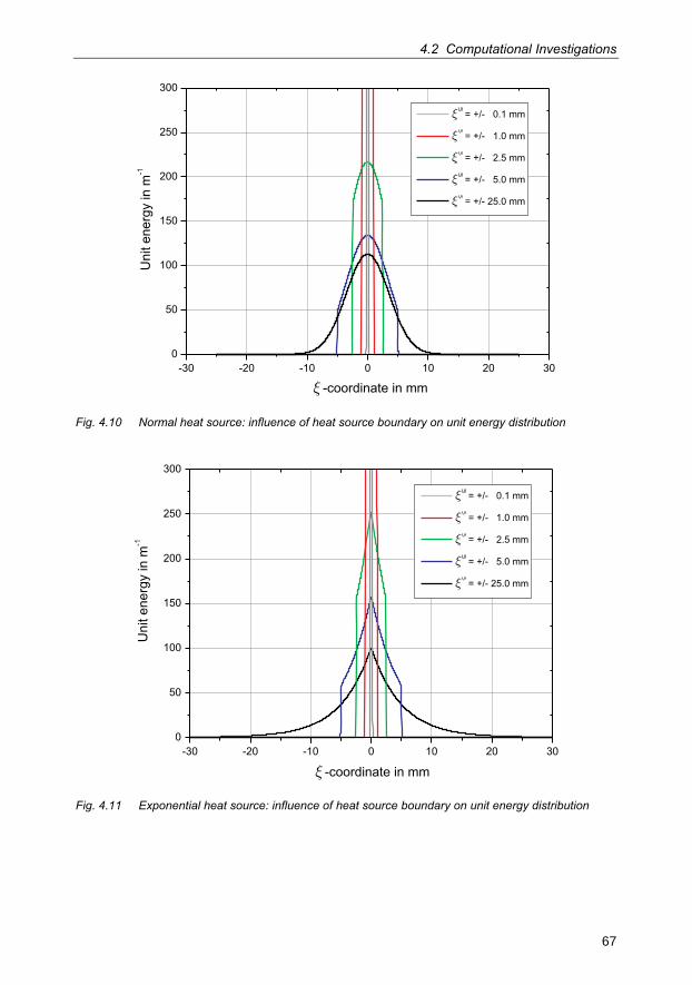
4.2 Computational Investigations
67
-30 -20 -10 0 10 20 300
50
100
150
200
250
300
Uni
tene
rgy
inm
-1
� -coordinate in mm
� = +/- 0.1 mm
� = +/- 1.0 mm
� = +/- 2.5 mm
� = +/- 5.0 mm
� = +/- 25.0 mm
,
,
,
,
,
Fig. 4.10 Normal heat source: influence of heat source boundary on unit energy distribution
-30 -20 -10 0 10 20 300
50
100
150
200
250
300
Uni
tene
rgy
inm
-1
� -coordinate in mm
� = +/- 0.1 mm
� = +/- 1.0 mm
� = +/- 2.5 mm
� = +/- 5.0 mm
� = +/- 25.0 mm
,
,
,
,
,
Fig. 4.11 Exponential heat source: influence of heat source boundary on unit energy distribution

4 Results
68 BAM-Dissertationsreihe
-30 -20 -10 0 10 20 300
50
100
150
200
250
300
Uni
tene
rgy
inm
-1
� = +/- 0.1 mm
� = +/- 1.0 mm
� = +/- 2.5 mm
� = +/- 5.0 mm
� = +/- 25.0 mm
,
,
,
,
,
� -coordinate in mm
Fig. 4.12 Parabolic heat source: influence of heat source boundary on unit energy distribution
Furthermore, the influences of different heat source distribution parameters have been studied. The results of a variation of the parameter ex for the normal and exponential dis-tribution are shown in Fig. 4.13 and Fig. 4.14 with a truncation at 250 m-1 concerning the unit energy f ( )x .
-20 -15 -10 -5 0 5 10 15 200
50
100
150
200
250
�e
= 0.1 mm
�e
= 1.0 mm
�e
= 2.5 mm
�e
= 5.0 mm
�e
= 25.0 mm
Uni
tene
rgy
inm
-1
� -coordinate in mm
Fig. 4.13 Influence of normal energy distribution parameter on the unit energy distribution
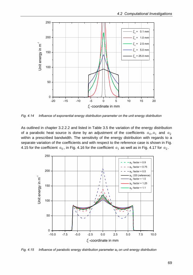
4.2 Computational Investigations
69
-20 -15 -10 -5 0 5 10 15 200
50
100
150
200
250
�e
0.1 mm
�e
1.0 mm
�e
2.5 mm
�e
5.0 mm
�e25.0 mm
Uni
tene
rgy
inm
-1
�e
= 0.1 mm
�e
= 1.0 mm
�e
= 2.5 mm
�e
= 5.0 mm
�e
= 25.0 mm
� -coordinate in mm
Fig. 4.14 Influence of exponential energy distribution parameter on the unit energy distribution
As outlined in chapter 3.2.2.2 and listed in Table 3.5 the variation of the energy distribution of a parabolic heat source is done by an adjustment of the coefficients a a0 1, and a2 within a prescribed bandwidth. The sensitivity of the energy distribution with regards to a separate variation of the coefficients and with respect to the reference case is shown in Fig. 4.15 for the coefficient a0 , in Fig. 4.16 for the coefficient a1 as well as in Fig. 4.17 for a2 .
-10.0 -7.5 -5.0 -2.5 0.0 2.5 5.0 7.5 10.00
50
100
150
200
250
a : factor = 1.50
a : factor = 1.250
a : factor = 1.10
a : 220 (reference)0
a : factor = 0.90
a : factor = 0.750
a : factor = 0.50
Uni
tene
rgy
inm
-1
� -coordinate in mm
Fig. 4.15 Influence of parabolic energy distribution parameter a0 on unit energy distribution
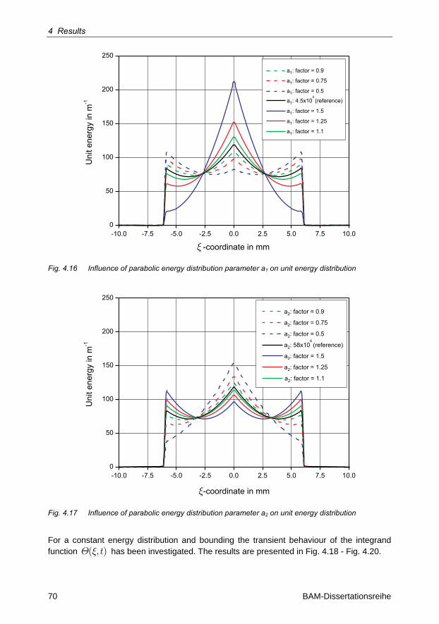
4 Results
70 BAM-Dissertationsreihe
-10.0 -7.5 -5.0 -2.5 0.0 2.5 5.0 7.5 10.00
50
100
150
200
250
a : factor = 1.51
a : factor = 1.251
a : factor = 1.11
a : 4.5x10¹⁴(reference)
a : factor = 0.91
a : factor = 0.751
a : factor = 0.51U
nite
nerg
yin
m-1
� -coordinate in mm
Fig. 4.16 Influence of parabolic energy distribution parameter a1 on unit energy distribution
-10.0 -7.5 -5.0 -2.5 0.0 2.5 5.0 7.5 10.00
50
100
150
200
250
a : factor = 1.52
a : factor = 1.252
a : factor = 1.12
a : 58x1026(reference)
a : factor = 0.92
a : factor = 0.752
a : factor = 0.52
Uni
tene
rgy
inm
-1
�-coordinate in mm
Fig. 4.17 Influence of parabolic energy distribution parameter a2 on unit energy distribution
For a constant energy distribution and bounding the transient behaviour of the integrand function t( , )Q x has been investigated. The results are presented in Fig. 4.18 - Fig. 4.20.
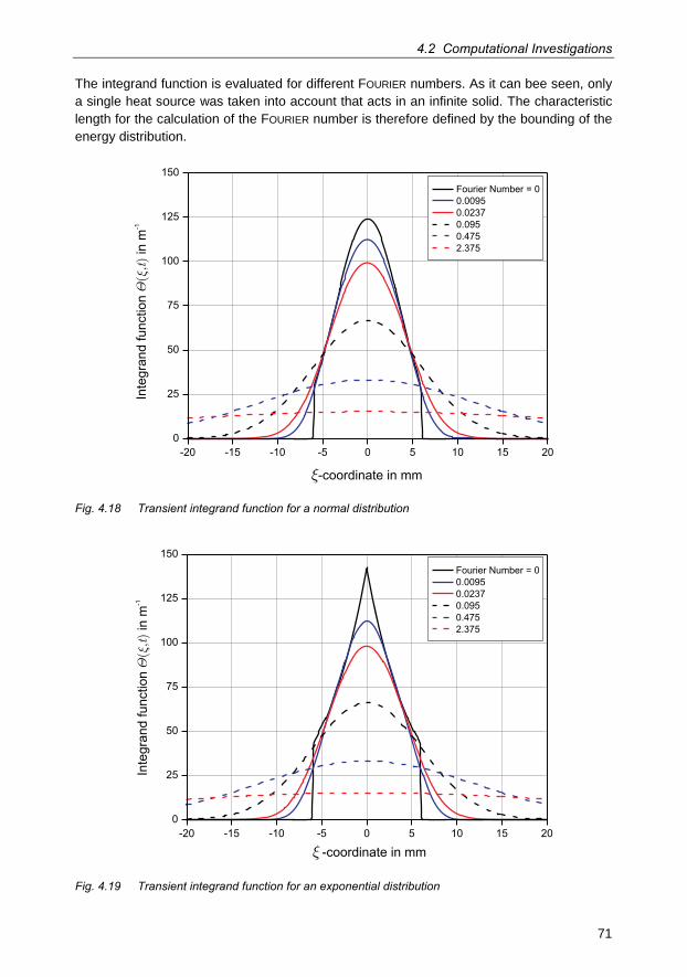
4.2 Computational Investigations
71
The integrand function is evaluated for different FOURIER numbers. As it can bee seen, only a single heat source was taken into account that acts in an infinite solid. The characteristic length for the calculation of the FOURIER number is therefore defined by the bounding of the energy distribution.
-20 -15 -10 -5 0 5 10 15 200
25
50
75
100
125
150Fourier Number = 00.00950.02370.0950.4752.375
�-coordinate in mm
Inte
gran
d fu
nctio
nin
m�
�(,)t
-1
Fig. 4.18 Transient integrand function for a normal distribution
-20 -15 -10 -5 0 5 10 15 200
25
50
75
100
125
150Fourier Number = 00.00950.02370.0950.4752.375
� -coordinate in mm
Inte
gran
d fu
nctio
nin
m�
�(,)t
-1
Fig. 4.19 Transient integrand function for an exponential distribution
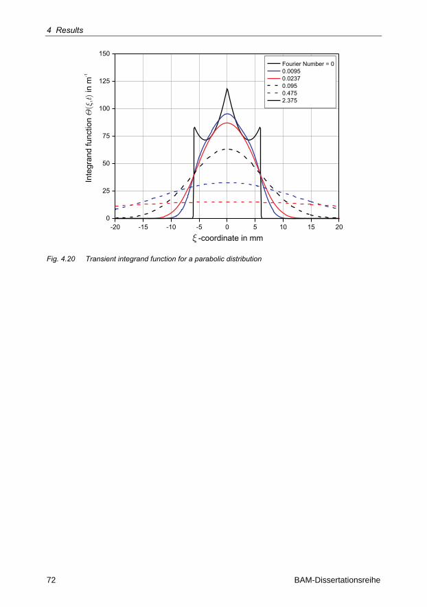
4 Results
72 BAM-Dissertationsreihe
-20 -15 -10 -5 0 5 10 15 200
25
50
75
100
125
150Fourier Number = 00.00950.02370.0950.4752.375
Inte
gran
d fu
nctio
nin
m�
�(,)t
-1
� -coordinate in mm
Fig. 4.20 Transient integrand function for a parabolic distribution
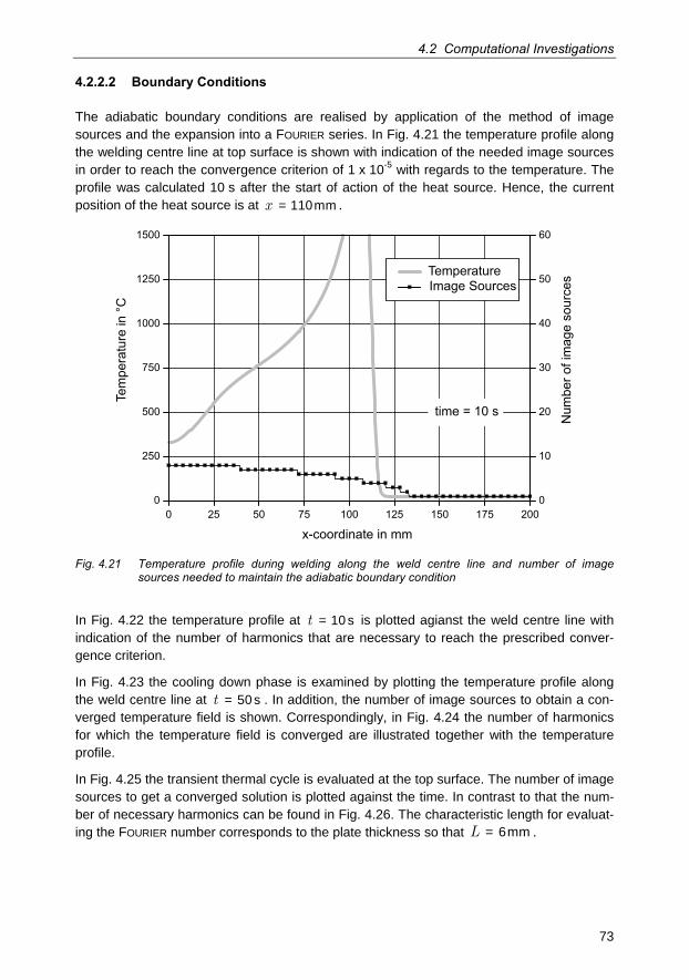
4.2 Computational Investigations
73
4.2.2.2 Boundary Conditions
The adiabatic boundary conditions are realised by application of the method of image sources and the expansion into a FOURIER series. In Fig. 4.21 the temperature profile along the welding centre line at top surface is shown with indication of the needed image sources in order to reach the convergence criterion of 1 x 10⁻⁵ with regards to the temperature. The profile was calculated 10 s after the start of action of the heat source. Hence, the current position of the heat source is at x = 110mm .
0 25 50 75 100 125 150 175 2000
250
500
750
1000
1250
1500
x-coordinate in mm
0
10
20
30
40
50
60
TemperatureImage Sources
time = 10 s Num
ber o
f im
age
sour
ces
Tem
pera
ture
in °
C
Fig. 4.21 Temperature profile during welding along the weld centre line and number of image sources needed to maintain the adiabatic boundary condition
In Fig. 4.22 the temperature profile at t = 10 s is plotted agianst the weld centre line with indication of the number of harmonics that are necessary to reach the prescribed conver-gence criterion.
In Fig. 4.23 the cooling down phase is examined by plotting the temperature profile along the weld centre line at t = 50 s . In addition, the number of image sources to obtain a con-verged temperature field is shown. Correspondingly, in Fig. 4.24 the number of harmonics for which the temperature field is converged are illustrated together with the temperature profile.
In Fig. 4.25 the transient thermal cycle is evaluated at the top surface. The number of image sources to get a converged solution is plotted against the time. In contrast to that the num-ber of necessary harmonics can be found in Fig. 4.26. The characteristic length for evaluat-ing the FOURIER number corresponds to the plate thickness so that L = 6mm .
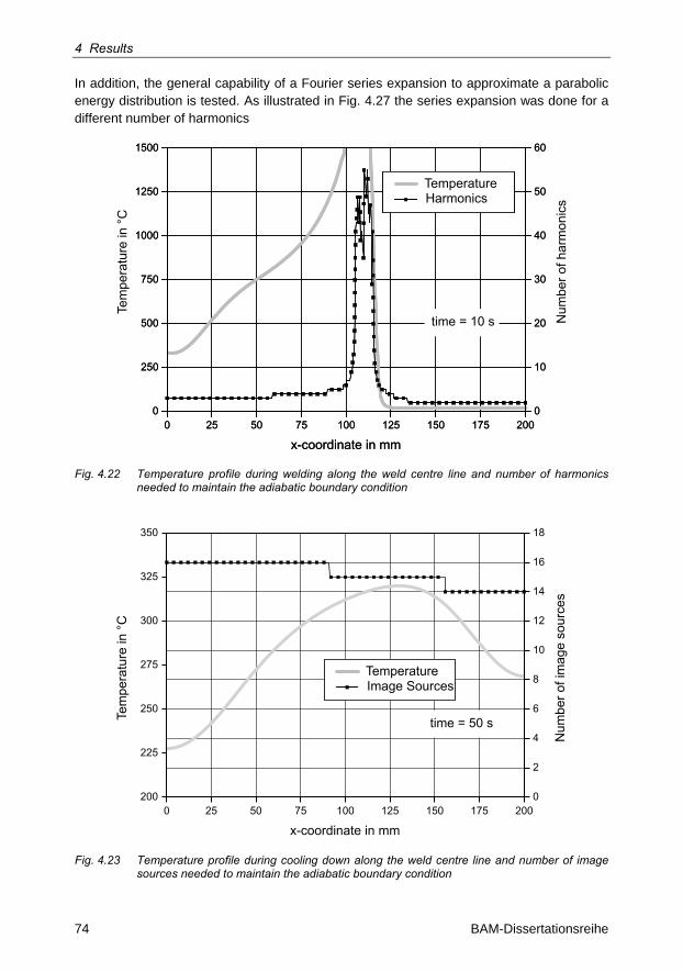
4 Results
74 BAM-Dissertationsreihe
In addition, the general capability of a Fourier series expansion to approximate a parabolic energy distribution is tested. As illustrated in Fig. 4.27 the series expansion was done for a different number of harmonics
0 25 50 75 100 125 150 175 2000
250
500
750
1000
1250
1500
x-coordinate in mm
0
10
20
30
40
50
60
Num
ber o
f har
mon
ics
Tem
pera
ture
in °
C
time = 10 s
TemperatureHarmonics
0 25 50 75 100 125 150 175 2000
250
500
750
1000
1250
1500
x-coordinate in mm
0
10
20
30
40
50
60
time = 10 s
TemperatureHarmonics
Fig. 4.22 Temperature profile during welding along the weld centre line and number of harmonics needed to maintain the adiabatic boundary condition
0 25 50 75 100 125 150 175 200200
225
250
275
300
325
350
x-coordinate in mm
0
2
4
6
8
10
12
14
16
18
Tem
pera
ture
in °
C
Num
ber o
f im
age
sour
ces
TemperatureImage Sources
time = 50 s
Fig. 4.23 Temperature profile during cooling down along the weld centre line and number of image sources needed to maintain the adiabatic boundary condition
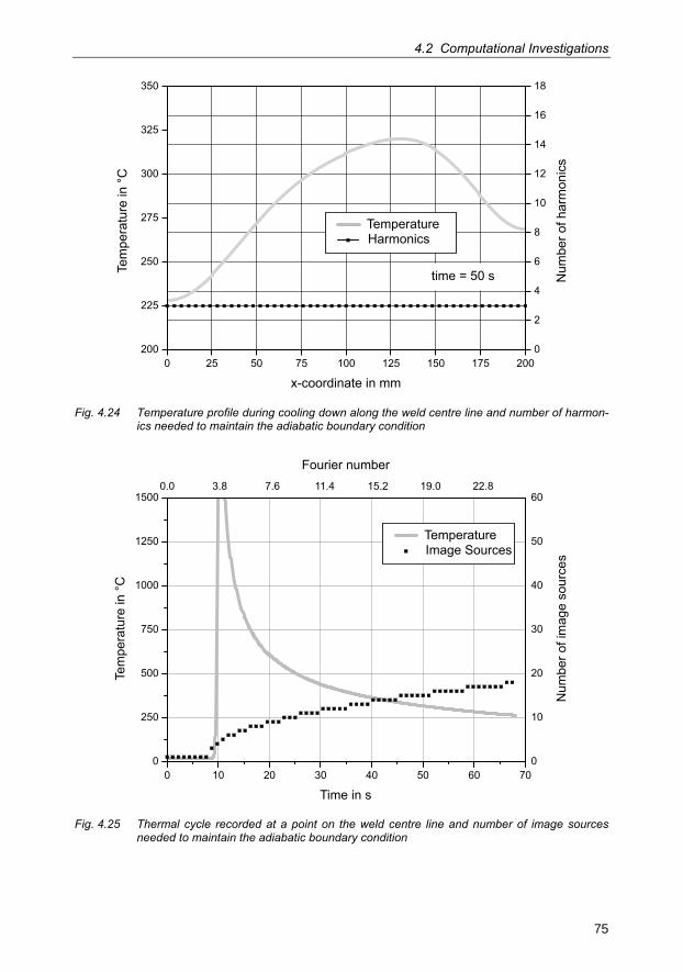
4.2 Computational Investigations
75
0 25 50 75 100 125 150 175 200200
225
250
275
300
325
350
x-coordinate in mm
0
2
4
6
8
10
12
14
16
18
Tem
pera
ture
in °
C
Num
ber o
f har
mon
ics
TemperatureHarmonics
time = 50 s
Fig. 4.24 Temperature profile during cooling down along the weld centre line and number of harmon-ics needed to maintain the adiabatic boundary condition
0 10 20 30 40 50 60 700
250
500
750
1000
1250
1500
Time in s
0
10
20
30
40
50
600.0 3.8 7.6 11.4 15.2 19.0 22.8
Fourier number
Num
ber o
f im
age
sour
ces
Tem
pera
ture
in °
C
TemperatureImage Sources
Fig. 4.25 Thermal cycle recorded at a point on the weld centre line and number of image sources needed to maintain the adiabatic boundary condition
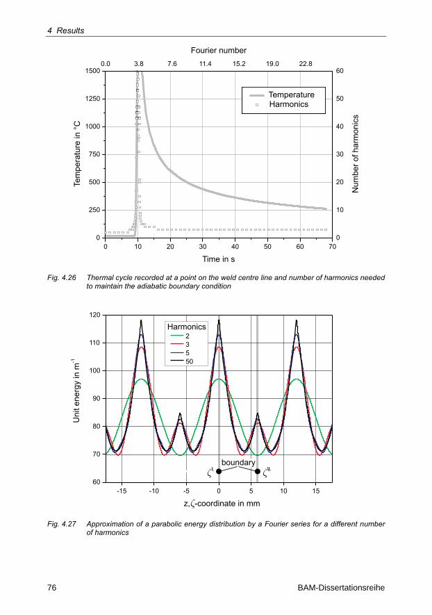
4 Results
76 BAM-Dissertationsreihe
0 10 20 30 40 50 60 700
250
500
750
1000
1250
1500
Time in s
0
10
20
30
40
50
600.0 3.8 7.6 11.4 15.2 19.0 22.8
Fourier number
Num
ber o
f har
mon
ics
Tem
pera
ture
in °
C
TemperatureHarmonicsTemperatureHarmonics
Fig. 4.26 Thermal cycle recorded at a point on the weld centre line and number of harmonics needed to maintain the adiabatic boundary condition
-15 -10 -5 0 5 10 1560
70
80
90
100
110
120
Uni
tene
rgy
inm
-1
z, -coordinate in mm�
boundary
23550
Harmonics
� �
Fig. 4.27 Approximation of a parabolic energy distribution by a Fourier series for a different number of harmonics
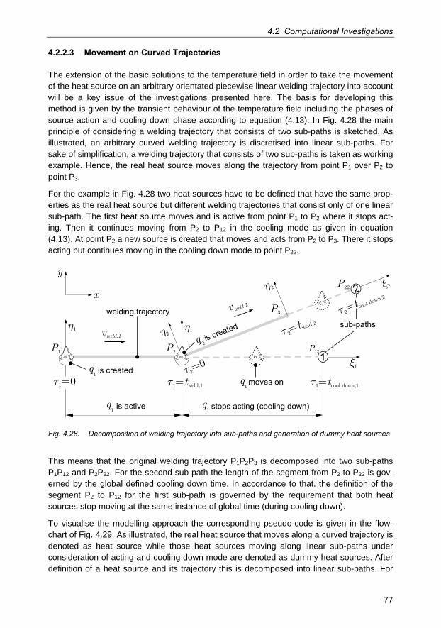
4.2 Computational Investigations
77
4.2.2.3 Movement on Curved Trajectories
The extension of the basic solutions to the temperature field in order to take the movement of the heat source on an arbitrary orientated piecewise linear welding trajectory into account will be a key issue of the investigations presented here. The basis for developing this method is given by the transient behaviour of the temperature field including the phases of source action and cooling down phase according to equation (4.13). In Fig. 4.28 the main principle of considering a welding trajectory that consists of two sub-paths is sketched. As illustrated, an arbitrary curved welding trajectory is discretised into linear sub-paths. For sake of simplification, a welding trajectory that consists of two sub-paths is taken as working example. Hence, the real heat source moves along the trajectory from point P1 over P2 to point P3.
For the example in Fig. 4.28 two heat sources have to be defined that have the same prop-erties as the real heat source but different welding trajectories that consist only of one linear sub-path. The first heat source moves and is active from point P1 to P2 where it stops act-ing. Then it continues moving from P2 to P12 in the cooling mode as given in equation (4.13). At point P2 a new source is created that moves and acts from P2 to P3. There it stops acting but continues moving in the cooling down mode to point P22.
vweld,1
�1
�1=0 �1 weld,1=t
�1
� 2
� 2
�1
vweld,2
� 2
� 2weld,2
=t
� 2=0
x
y
2
welding trajectorysub-paths
stops acting (cooling down)
P1 P2
P3
P12
P22
�1 cool down,1=t
� 2coo
l down,2
=t
1
q1
q1
is active
q1
is created
q 2is created
moves onq1
Fig. 4.28: Decomposition of welding trajectory into sub-paths and generation of dummy heat sources
This means that the original welding trajectory P1P2P3 is decomposed into two sub-paths P1P12 and P2P22. For the second sub-path the length of the segment from P2 to P22 is gov-erned by the global defined cooling down time. In accordance to that, the definition of the segment P2 to P12 for the first sub-path is governed by the requirement that both heat sources stop moving at the same instance of global time (during cooling down).
To visualise the modelling approach the corresponding pseudo-code is given in the flow-chart of Fig. 4.29. As illustrated, the real heat source that moves along a curved trajectory is denoted as heat source while those heat sources moving along linear sub-paths under consideration of acting and cooling down mode are denoted as dummy heat sources. After definition of a heat source and its trajectory this is decomposed into linear sub-paths. For
4 Results
78 BAM-Dissertationsreihe
each sub-path a dummy heat source is created and a corresponding path of movement is assigned. This new and now linear welding path includes a segment where the heat source acts and a segment where it stops acting but virtually moves on. As mentioned, the length of the previous one is governed by the globally defined cooling time and the total number of sub-paths. In order to simplify the method described above, the introduction of a local and global time frame is done. Therefore, a local time scale is defined for each dummy heat source. In Fig. 4.28 the local time variable is denoted as nt where the index n corre-sponds to the number of the sub-path under investigation. The integration with respect to time is then performed for the local time variable nt which corresponds again to the time of heat diffusion as requested in equation (4.13). For the dummy heat source dummyq1, at time nt and during its time of action this yields the following time integral to be solved:
weld,tdummyq
T x,y,z t x y zc
11,
1 1 1 1 1
0
( , ) = ( , ) ( , ) ( , ) dQ t Q t Q t tr ò (4.40)
while for the segment of cooling the subsequent integral has to be evaluated:
cd
cd weld
tdummy
t t
qT x,y,z t x y z
c
,1
,1 ,1
1,1 1 1 1 1( , ) = ( , ) ( , ) ( , ) dQ t Q t Q t t
r-ò (4.41)
where the index cd,1 stands for the cooling down time of the first heat source.
The local time of heat diffusion for each dummy heat source always starts with zero and ends with its specific cooling down time for its own sub-segment of the welding trajectory. At the same time, the global time flows continuously. Thus, a global start and finish time is assigned to each dummy heat source. With respect to the illustrating example presented in Fig. 4.28 the global start time for the first source is zero and the global finish time is
finish cool downt t,1 ,1= . For the second source the global start time is defined as
start weldt t,2 ,1= and the global finish time finish cool downt t,2 ,2= . This can be cast into an equation as follows:
finish n
start n
tN
nn t
T x,y,z t T x y z t
,
,1
( , ) = ( , , , )=å (4.42)
that fulfils the requirement of modelling the movement of a heat source along an arbitrary welding trajectory consisting of N linear sub-paths.
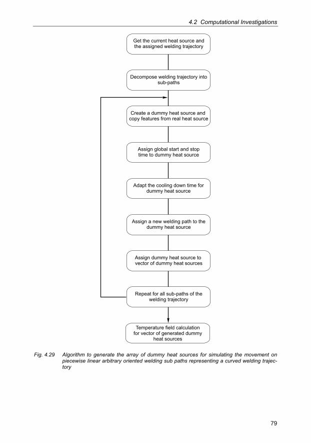
4.2 Computational Investigations
79
Get the current heat source andthe assigned welding trajectory
Create a dummy heat source andcopy features from real heat source
Adapt the cooling down time fordummy heat source
Assign a new welding path to thedummy heat source
Assign dummy heat source tovector of dummy heat sources
Repeat for all sub-paths of thewelding trajectory
Decompose welding trajectory intosub-paths
Assign global start and stoptime to dummy heat source
Temperature field calculationfor vector of generated dummy
heat sources
Fig. 4.29 Algorithm to generate the array of dummy heat sources for simulating the movement on piecewise linear arbitrary oriented welding sub paths representing a curved welding trajec-tory
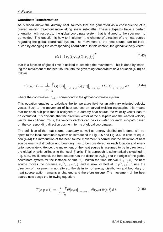
4 Results
80 BAM-Dissertationsreihe
Coordinate Transformation As outlined above the dummy heat sources that are generated as a consequence of a curved welding trajectory move along linear sub-paths. These sub-paths have a certain orientation with respect to the global coordinate system that is aligned to the specimen to be welded. The question is how to implement the change of direction of the heat source regarding the global coordinate system. The movement of the heat source can be intro-duced by changing the corresponding coordinates. In this context, the global velocity vector
( )Tx y zt v t v t v t( ) ( ), ( ), ( )=v (4.43)
that is a function of global time is utilised to describe the movement. This is done by insert-ing the movement of the heat source into the governing temperature field equation (4.10) as follows
x y z
t
x x v t y y v t z z v t
qT x y z t x t y t z t t
c0
( , , , ) = ( , ) ( , ) ( , ) dQ Q Qr + + +ò (4.44)
where the coordinates x y z, , correspond to the global coordinate system.
This equation enables to calculate the temperature field for an arbitrary oriented velocity vector. Back to the movement of heat sources on curved welding trajectories this means that for each sub-path that is assigned to a dummy heat source the velocity vector has to be evaluated. It is obvious, that the direction vector of the sub-path and the wanted velocity vector are collinear. Thus, the velocity vectors can be calculated for each sub-path based on the corresponding direction cosine in terms of global coordinates.
The definition of the heat source boundary as well as energy distribution is done with re-spect to the local coordinate system as introduced in Fig. 3.5 and Fig. 3.6. In case of equa-tion (4.44) the introduction of the heat source movement is correct but the definition of heat source energy distribution and boundary has to be considered for each location and orien-tation separately. Hence, the movement of the heat source is assumed to be in direction of the global x -axis collinear to the local x axis. This approach is schematically sketched in Fig. 4.30. As illustrated, the heat source has the distance nx t0( ) to the origin of the global coordinate system for the instance of time nt . Within the time interval n nt t+1 - the heat source moves the distance x n nv t t+1( - ) and is now located at nx t0 1( )+ . Since the direction of movement is not altered, the definition of energy distribution and boundary of heat source action remains unchanged and therefore unique. The movement of the heat source now obeys the following equation:
x
t
x x v t
qT x y z t x t y t z t t
c0
( , , , ) = ( , ) ( , ) ( , ) dQ Q Qr +ò (4.45)
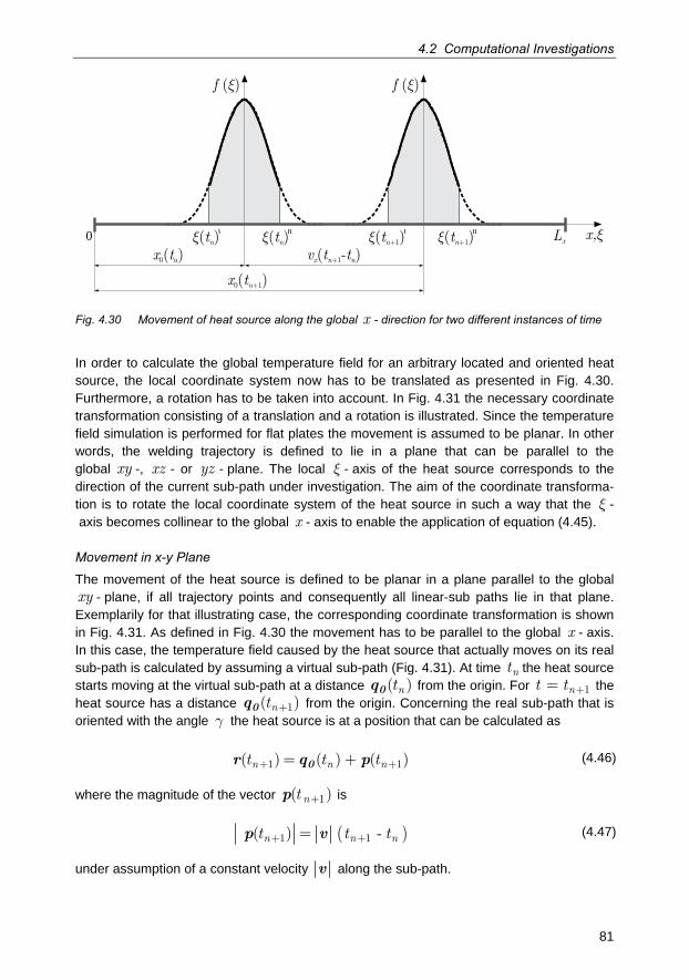
4.2 Computational Investigations
81
x t0 n( )
0 Lxx��
f ( )� f ( )�
x t0 +1( )n
�( )tn+1
/
v t tx n n( - )+1
�( )tn
/�( )tn
/ /�( )tn+1
/ /
Fig. 4.30 Movement of heat source along the global x - direction for two different instances of time
In order to calculate the global temperature field for an arbitrary located and oriented heat source, the local coordinate system now has to be translated as presented in Fig. 4.30. Furthermore, a rotation has to be taken into account. In Fig. 4.31 the necessary coordinate transformation consisting of a translation and a rotation is illustrated. Since the temperature field simulation is performed for flat plates the movement is assumed to be planar. In other words, the welding trajectory is defined to lie in a plane that can be parallel to the global xy -, xz - or yz - plane. The local x - axis of the heat source corresponds to the direction of the current sub-path under investigation. The aim of the coordinate transforma-tion is to rotate the local coordinate system of the heat source in such a way that the x - axis becomes collinear to the global x - axis to enable the application of equation (4.45).
Movement in x-y Plane
The movement of the heat source is defined to be planar in a plane parallel to the global xy - plane, if all trajectory points and consequently all linear-sub paths lie in that plane. Exemplarily for that illustrating case, the corresponding coordinate transformation is shown in Fig. 4.31. As defined in Fig. 4.30 the movement has to be parallel to the global x - axis. In this case, the temperature field caused by the heat source that actually moves on its real sub-path is calculated by assuming a virtual sub-path (Fig. 4.31). At time nt the heat source starts moving at the virtual sub-path at a distance nt( )0q from the origin. For nt t 1+= the heat source has a distance nt 1( )+0q from the origin. Concerning the real sub-path that is oriented with the angle g the heat source is at a position that can be calculated as
n n nt t t1 1( ) ( ) ( )+ += +0r q p (4.46)
where the magnitude of the vector nt 1( )+p is
( )n n nt t t1 1( ) -+ +=p v (4.47)
under assumption of a constant velocity v along the sub-path.
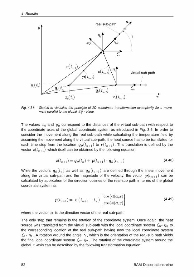
4 Results
82 BAM-Dissertationsreihe
x
y
r( )tn+1
�1
�1
� 2
real sub-path
q0 n( )t
p( )tn+1
x t0 n( )
virtual sub-path
� 2
x t0 n+1( )
q0 n+1( )t
s( )tn+1
� 0
�0
y t0 n( )
a
Fig. 4.31 Sketch to visualise the principle of 2D coordinate transformation exemplarily for a move-ment parallel to the global xy - plane
The values x 0 and y0 correspond to the distances of the virtual sub-path with respect to the coordinate axes of the global coordinate system as introduced in Fig. 3.6. In order to consider the movement along the real sub-path while calculating the temperature field by assuming the movement along the virtual sub-path, the heat source has to be translated for each time step from the location nt 1( )+0q to nt 1( )+r . This translation is defined by the vector nt 1( )+s which itself can be obtained by the following equation
n n n nt t t t1 1 1( ) ( ) ( ) - ( )+ + += +0 0s q p q (4.48)
While the vectors nt( )0q as well as nt 1( )+0q are defined through the linear movement along the virtual sub-path and the magnitude of the velocity, the vector nt 1( )+p can be calculated by application of the direction cosines of the real-sub path in terms of the global coordinate system as
( )n n n
xt t t
y1 1
cos( ( , )( )
cos( ( , )+ +
ì üï ïï ï= - í ýï ïï ïî þ
ap v
a
(4.49)
where the vector a is the direction vector of the real sub-path.
The only step that remains is the rotation of the coordinate system. Once again, the heat source was translated from the virtual sub-path with the local coordinate system -0 0x h to the corresponding location at the real sub-path having now the local coordinate system
-1 1x h . A rotation around the angle g , which is the orientation of the real-sub path yields the final local coordinate system -2 2x h . The rotation of the coordinate system around the global z -axis can be described by the following transformation equation:
4.2 Computational Investigations
83
2 1
2 1
2 1
cos sin 0
sin cos 0
0 0 1
x g g xh g g hz z
ì ü é ù ì üï ï ï ïï ï ï ïê úï ï ï ïï ï ï ïê ú= -í ý í ýê úï ï ï ïï ï ï ïê úï ï ï ïê úï ï ï ïî þ ë û î þ
(4.50)
realising that the z -component remains unchanged as requested in case of the moving in the x-y -plane.
Movement in x-z Plane
If the heat source moves in a plane parallel to the x-z -plane then the process of coordi-nate transformation has to be done accordingly. Here only the different rotation of the coor-dinate system is presented. This is given by a rotation around the y- axis as:
2 1
2 1
2 1
cos 0 sin
0 1 0
sin 0 cos
x b b xh hz b b z
ì ü é ù ì üï ï ï ïï ï ï ïê úï ï ï ïï ï ï ïê ú=í ý í ýê úï ï ï ïï ï ï ïê ú-ï ï ï ïê úï ï ï ïî þ ë û î þ
(4.51)
where the angle b defines the orientation of the real sub-path with respect to the x-z -plane so is the angle between direction vector of the real sub-path and the global x- axis.
Movement in y-z Plane
The heat source can also move within a plane parallel to the global y-z -plane. As men-tioned the basic approach of the coordinate transformation is the same consisting of a translation and rotation to transform the -1 1x h coordinate system into the -2 2x h system. However, as defined above the requirement is that the heat source moves along a virtual sub-path which is parallel to the global x- axis. This means that the coordinate system of the heat source has to be rotated in two steps. At first, the local -1 1x h system is rotated by
/ 2g p= around the global z- axis so that the local -1x axis coincides with the global y- axis. Then the rotation around the x- axis with the angle a is performed that corre-sponds to the angle of the real sub-path with the global y- axis. The complete coordinate rotation obeys the following equation
2 1
2 1
2 1
cos - sin cos - sin sin
sin cos cos cos sin
0 - sin cos
x g g a g a xh g g a g a hz a a z
ì ü é ù ì üï ï ï ïï ï ï ïê úï ï ï ïï ï ï ïê ú=í ý í ýê úï ï ï ïï ï ï ïê úï ï ï ïê úï ï ï ïî þ ë û î þ
(4.52)
Movement on Three Dimensional Trajectory
Theoretically, the movement along a three dimensional welding trajectory can also be con-sidered. As illustrated in Fig. 4.32 the - -1 1 1x h z coordinate system is oriented so that its local 1x -axis is parallel to the global x -axis. The transformation from the - -1 1 1x h z coordi-nate system to the - -2 2 2x h z -system can be done by translation and rotation as described above for the case of planar trajectories. The orientation of the coordinate system that is
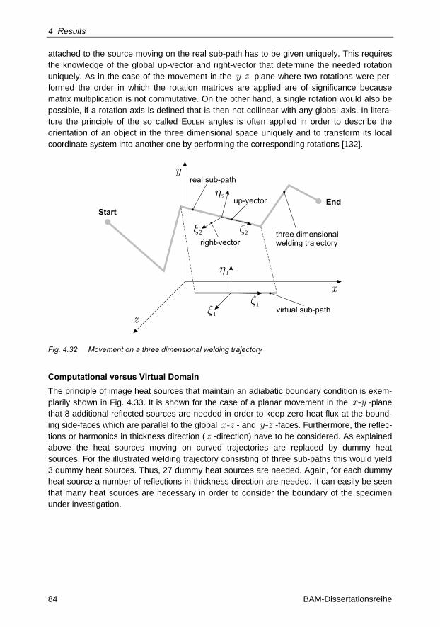
4 Results
84 BAM-Dissertationsreihe
attached to the source moving on the real sub-path has to be given uniquely. This requires the knowledge of the global up-vector and right-vector that determine the needed rotation uniquely. As in the case of the movement in the y-z -plane where two rotations were per-formed the order in which the rotation matrices are applied are of significance because matrix multiplication is not commutative. On the other hand, a single rotation would also be possible, if a rotation axis is defined that is then not collinear with any global axis. In litera-ture the principle of the so called EULER angles is often applied in order to describe the orientation of an object in the three dimensional space uniquely and to transform its local coordinate system into another one by performing the corresponding rotations [132].
�1
�1
�2
�2
�1
�2
x
y
z
real sub-path
virtual sub-path
right-vector
up-vector
three dimensionalwelding trajectory
Start
End
Fig. 4.32 Movement on a three dimensional welding trajectory
Computational versus Virtual Domain The principle of image heat sources that maintain an adiabatic boundary condition is exem-plarily shown in Fig. 4.33. It is shown for the case of a planar movement in the x-y -plane that 8 additional reflected sources are needed in order to keep zero heat flux at the bound-ing side-faces which are parallel to the global x-z - and y-z -faces. Furthermore, the reflec-tions or harmonics in thickness direction ( z -direction) have to be considered. As explained above the heat sources moving on curved trajectories are replaced by dummy heat sources. For the illustrated welding trajectory consisting of three sub-paths this would yield 3 dummy heat sources. Thus, 27 dummy heat sources are needed. Again, for each dummy heat source a number of reflections in thickness direction are needed. It can easily be seen that many heat sources are necessary in order to consider the boundary of the specimen under investigation.
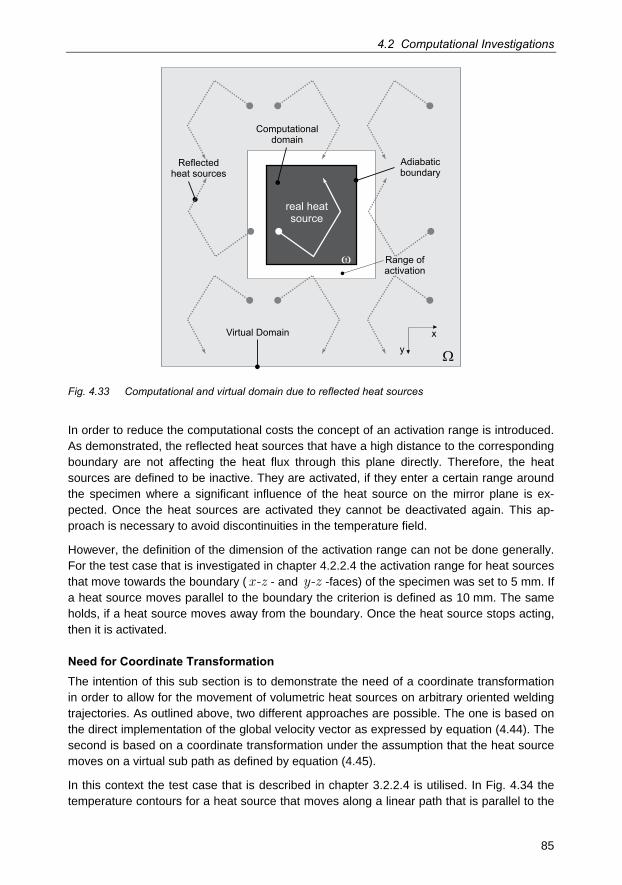
4.2 Computational Investigations
85
Computationaldomain
Virtual Domain
�
Adiabaticboundary
Reflectedheat sources
�
real heatsource
Range ofactivation
xy
Fig. 4.33 Computational and virtual domain due to reflected heat sources
In order to reduce the computational costs the concept of an activation range is introduced. As demonstrated, the reflected heat sources that have a high distance to the corresponding boundary are not affecting the heat flux through this plane directly. Therefore, the heat sources are defined to be inactive. They are activated, if they enter a certain range around the specimen where a significant influence of the heat source on the mirror plane is ex-pected. Once the heat sources are activated they cannot be deactivated again. This ap-proach is necessary to avoid discontinuities in the temperature field.
However, the definition of the dimension of the activation range can not be done generally. For the test case that is investigated in chapter 4.2.2.4 the activation range for heat sources that move towards the boundary (x-z - and y-z -faces) of the specimen was set to 5 mm. If a heat source moves parallel to the boundary the criterion is defined as 10 mm. The same holds, if a heat source moves away from the boundary. Once the heat source stops acting, then it is activated.
Need for Coordinate Transformation The intention of this sub section is to demonstrate the need of a coordinate transformation in order to allow for the movement of volumetric heat sources on arbitrary oriented welding trajectories. As outlined above, two different approaches are possible. The one is based on the direct implementation of the global velocity vector as expressed by equation (4.44). The second is based on a coordinate transformation under the assumption that the heat source moves on a virtual sub path as defined by equation (4.45).
In this context the test case that is described in chapter 3.2.2.4 is utilised. In Fig. 4.34 the temperature contours for a heat source that moves along a linear path that is parallel to the
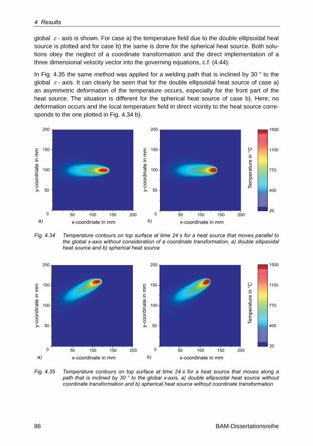
4 Results
86 BAM-Dissertationsreihe
global x - axis is shown. For case a) the temperature field due to the double ellipsoidal heat source is plotted and for case b) the same is done for the spherical heat source. Both solu-tions obey the neglect of a coordinate transformation and the direct implementation of a three dimensional velocity vector into the governing equations, c.f. (4.44).
In Fig. 4.35 the same method was applied for a welding path that is inclined by 30 ° to the global x - axis. It can clearly be seen that for the double ellipsoidal heat source of case a) an asymmetric deformation of the temperature occurs, especially for the front part of the heat source. The situation is different for the spherical heat source of case b). Here, no deformation occurs and the local temperature field in direct vicinity to the heat source corre-sponds to the one plotted in Fig. 4.34 b).
0
50
100
150
200
y-co
ordi
nate
in m
m
50 100 150 200
x-coordinate in mma)
20
400
770
1100
1500
Tem
pera
ture
in °
C
0
50
100
150
200
y-co
ordi
nate
in m
m
50 100 150 200
x-coordinate in mmb)
Fig. 4.34 Temperature contours on top surface at time 24 s for a heat source that moves parallel to the global x-axis without consideration of a coordinate transformation, a) double ellipsoidal heat source and b) spherical heat source
0
50
100
150
200
y-co
ordi
nate
in m
m
50 100 150 200
x-coordinate in mma)
20
400
770
1100
1500
Tem
pera
ture
in °
C
b)0
50
100
150
200
y-co
ordi
nate
in m
m
50 100 150 200
x-coordinate in mm
Fig. 4.35 Temperature contours on top surface at time 24 s for a heat source that moves along a path that is inclined by 30 ° to the global x-axis, a) double ellipsoidal heat source without coordinate transformation and b) spherical heat source without coordinate transformation
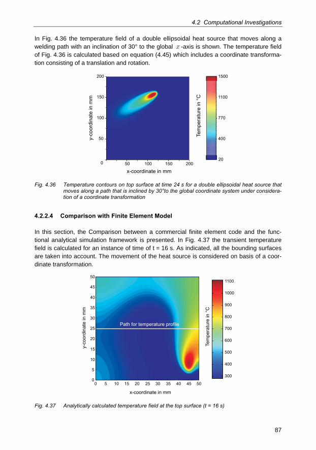
4.2 Computational Investigations
87
In Fig. 4.36 the temperature field of a double ellipsoidal heat source that moves along a welding path with an inclination of 30° to the global x -axis is shown. The temperature field of Fig. 4.36 is calculated based on equation (4.45) which includes a coordinate transforma-tion consisting of a translation and rotation.
20
400
770
1100
1500
Tem
pera
ture
in °
C
0
50
100
150
200
y-co
ordi
nate
in m
m
50 100 150 200
x-coordinate in mm
Fig. 4.36 Temperature contours on top surface at time 24 s for a double ellipsoidal heat source that moves along a path that is inclined by 30°to the global coordinate system under considera-tion of a coordinate transformation
4.2.2.4 Comparison with Finite Element Model
In this section, the Comparison between a commercial finite element code and the func-tional analytical simulation framework is presented. In Fig. 4.37 the transient temperature field is calculated for an instance of time of t = 16 s. As indicated, all the bounding surfaces are taken into account. The movement of the heat source is considered on basis of a coor-dinate transformation.
300
400
500
600
700
800
900
1000
1100
Tem
pera
ture
in °
C
0 5 10 15 20 25 30 35 40 45 50
x-coordinate in mm
0
5
10
15
20
25
30
35
40
45
50
y-co
ordi
nate
in m
m
Path for temperature profile
Fig. 4.37 Analytically calculated temperature field at the top surface (t = 16 s)
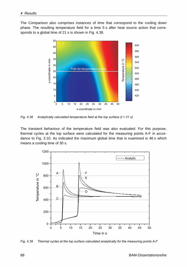
4 Results
88 BAM-Dissertationsreihe
The Comparison also comprises instances of time that correspond to the cooling down phase. The resulting temperature field for a time 5 s after heat source action that corre-sponds to a global time of 21 s is shown in Fig. 4.38.
420
440
460
480
500
520
540
560
580
600
Tem
pera
ture
in °
C
0 5 10 15 20 25 30 35 40 45 50
x-coordinate in mm
0
5
10
15
20
25
30
35
40
45
50
y-co
ordi
nate
in m
m
Path for temperature profile
Fig. 4.38 Analytically calculated temperature field at the top surface (t = 21 s)
The transient behaviour of the temperature field was also evaluated. For this purpose, thermal cycles at the top surface were calculated for the measuring points A-F in accor-dance to Fig. 3.10. As indicated the maximum global time that is examined is 46 s which means a cooling time of 30 s.
0 5 10 15 20 25 30 35 40 45 500
200
400
600
800
1000
1200
Analytic
Time in s
Tem
pera
ture
in °
C A
B
C
FE
D
Fig. 4.39 Thermal cycles at the top surface calculated analytically for the measuring points A-F
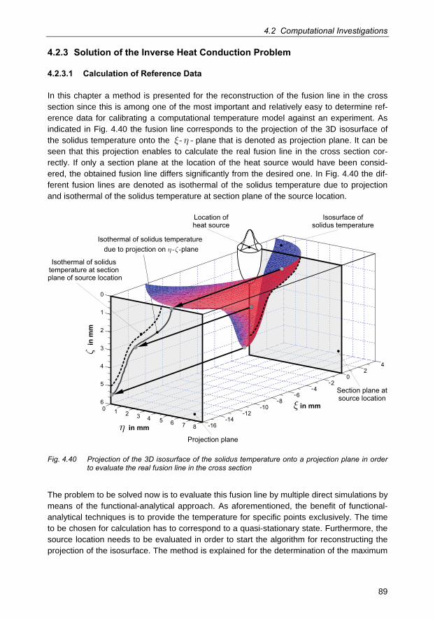
4.2 Computational Investigations
89
4.2.3 Solution of the Inverse Heat Conduction Problem
4.2.3.1 Calculation of Reference Data
In this chapter a method is presented for the reconstruction of the fusion line in the cross section since this is among one of the most important and relatively easy to determine ref-erence data for calibrating a computational temperature model against an experiment. As indicated in Fig. 4.40 the fusion line corresponds to the projection of the 3D isosurface of the solidus temperature onto the - -x h plane that is denoted as projection plane. It can be seen that this projection enables to calculate the real fusion line in the cross section cor-rectly. If only a section plane at the location of the heat source would have been consid-ered, the obtained fusion line differs significantly from the desired one. In Fig. 4.40 the dif-ferent fusion lines are denoted as isothermal of the solidus temperature due to projection and isothermal of the solidus temperature at section plane of the source location.
Projection plane
Isothermal of solidus temperaturedue to projection on plane� �- -
Isothermal of solidustemperature at sectionplane of source location
Section plane atsource location
� in mm
� in mm
�in
mm
Location ofheat source
Isosurface ofsolidus temperature
Fig. 4.40 Projection of the 3D isosurface of the solidus temperature onto a projection plane in order to evaluate the real fusion line in the cross section
The problem to be solved now is to evaluate this fusion line by multiple direct simulations by means of the functional-analytical approach. As aforementioned, the benefit of functional-analytical techniques is to provide the temperature for specific points exclusively. The time to be chosen for calculation has to correspond to a quasi-stationary state. Furthermore, the source location needs to be evaluated in order to start the algorithm for reconstructing the projection of the isosurface. The method is explained for the determination of the maximum
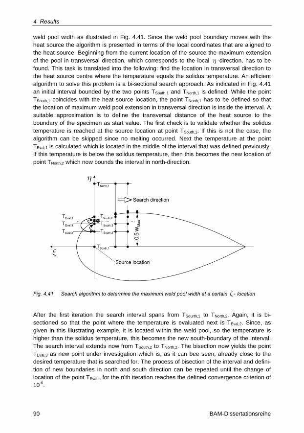
4 Results
90 BAM-Dissertationsreihe
weld pool width as illustrated in Fig. 4.41. Since the weld pool boundary moves with the heat source the algorithm is presented in terms of the local coordinates that are aligned to the heat source. Beginning from the current location of the source the maximum extension of the pool in transversal direction, which corresponds to the local h -direction, has to be found. This task is translated into the following: find the location in transversal direction to the heat source centre where the temperature equals the solidus temperature. An efficient algorithm to solve this problem is a bi-sectional search approach. As indicated in Fig. 4.41 an initial interval bounded by the two points TSouth,1 and TNorth,1 is defined. While the point TSouth,1 coincides with the heat source location, the point TNorth,1 has to be defined so that the location of maximum weld pool extension in transversal direction is inside the interval. A suitable approximation is to define the transversal distance of the heat source to the boundary of the specimen as start value. The first check is to validate whether the solidus temperature is reached at the source location at point TSouth,1. If this is not the case, the algorithm can be skipped since no melting occurred. Next the temperature at the point TEval,1 is calculated which is located in the middle of the interval that was defined previously. If this temperature is below the solidus temperature, then this becomes the new location of point TNorth,2 which now bounds the interval in north-direction.
�TNorth,1
TSouth,1
TNorth,2
TSouth,2
TEval,1
TEval,2
TEval,3 TSouth,3...
�
...
Search direction
0.5
wM
ax...
Source location
Fig. 4.41 Search algorithm to determine the maximum weld pool width at a certain -z location
After the first iteration the search interval spans from TSourth,1 to TNorth,2. Again, it is bi-sectioned so that the point where the temperature is evaluated next is TEval,2. Since, as given in this illustrating example, it is located within the weld pool, so the temperature is higher than the solidus temperature, this becomes the new south-boundary of the interval. The search interval extends now from TSouth,2 to TNorth,2. The bisection now yields the point TEval,3 as new point under investigation which is, as it can bee seen, already close to the desired temperature that is searched for. The process of bisection of the interval and defini-tion of new boundaries in north and south direction can be repeated until the change of location of the point TEval,n for the n’th iteration reaches the defined convergence criterion of 10-6.
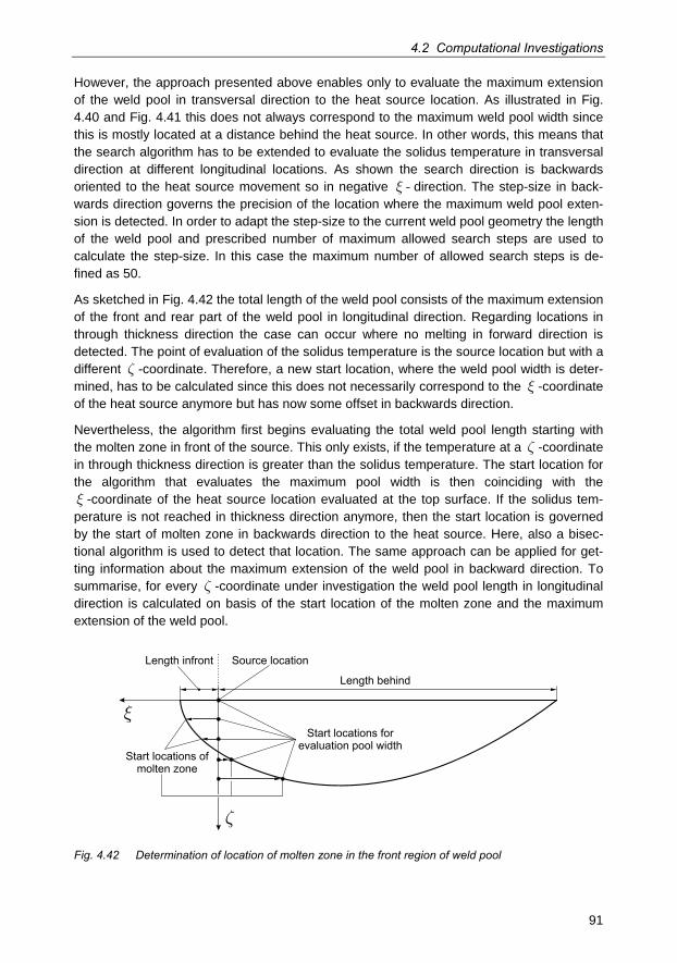
4.2 Computational Investigations
91
However, the approach presented above enables only to evaluate the maximum extension of the weld pool in transversal direction to the heat source location. As illustrated in Fig. 4.40 and Fig. 4.41 this does not always correspond to the maximum weld pool width since this is mostly located at a distance behind the heat source. In other words, this means that the search algorithm has to be extended to evaluate the solidus temperature in transversal direction at different longitudinal locations. As shown the search direction is backwards oriented to the heat source movement so in negative -x direction. The step-size in back-wards direction governs the precision of the location where the maximum weld pool exten-sion is detected. In order to adapt the step-size to the current weld pool geometry the length of the weld pool and prescribed number of maximum allowed search steps are used to calculate the step-size. In this case the maximum number of allowed search steps is de-fined as 50.
As sketched in Fig. 4.42 the total length of the weld pool consists of the maximum extension of the front and rear part of the weld pool in longitudinal direction. Regarding locations in through thickness direction the case can occur where no melting in forward direction is detected. The point of evaluation of the solidus temperature is the source location but with a different z -coordinate. Therefore, a new start location, where the weld pool width is deter-mined, has to be calculated since this does not necessarily correspond to the x -coordinate of the heat source anymore but has now some offset in backwards direction.
Nevertheless, the algorithm first begins evaluating the total weld pool length starting with the molten zone in front of the source. This only exists, if the temperature at a z -coordinate in through thickness direction is greater than the solidus temperature. The start location for the algorithm that evaluates the maximum pool width is then coinciding with the x -coordinate of the heat source location evaluated at the top surface. If the solidus tem-perature is not reached in thickness direction anymore, then the start location is governed by the start of molten zone in backwards direction to the heat source. Here, also a bisec-tional algorithm is used to detect that location. The same approach can be applied for get-ting information about the maximum extension of the weld pool in backward direction. To summarise, for every z -coordinate under investigation the weld pool length in longitudinal direction is calculated on basis of the start location of the molten zone and the maximum extension of the weld pool.
Length infront
Length behind
�
�
Source location
Start locations ofmolten zone
Start locations forevaluation pool width
Fig. 4.42 Determination of location of molten zone in the front region of weld pool
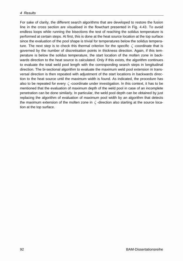
4 Results
92 BAM-Dissertationsreihe
For sake of clarity, the different search algorithms that are developed to restore the fusion line in the cross section are visualised in the flowchart presented in Fig. 4.43. To avoid endless loops while running the bisections the test of reaching the solidus temperature is performed at certain steps. At first, this is done at the heat source location at the top surface since the evaluation of the pool shape is trivial for temperatures below the solidus tempera-ture. The next step is to check this thermal criterion for the specific z -coordinate that is governed by the number of discretisation points in thickness direction. Again, if this tem-perature is below the solidus temperature, the start location of the molten zone in back-wards direction to the heat source is calculated. Only if this exists, the algorithm continues to evaluate the total weld pool length with the corresponding search steps in longitudinal direction. The bi-sectional algorithm to evaluate the maximum weld pool extension in trans-versal direction is then repeated with adjustment of the start locations in backwards direc-tion to the heat source until the maximum width is found. As indicated, the procedure has also to be repeated for every z -coordinate under investigation. In this context, it has to be mentioned that the evaluation of maximum depth of the weld pool in case of an incomplete penetration can be done similarly. In particular, the weld pool depth can be obtained by just replacing the algorithm of evaluation of maximum pool width by an algorithm that detects the maximum extension of the molten zone in z -direction also starting at the source loca-tion at the top surface.
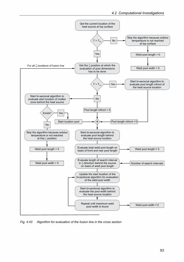
4.2 Computational Investigations
93
Get the current location of theheat source at top surface
Get the -position at which theevaluation of pool dimensions
has to be done
�
No
+
Start bi-secional algorithm toevaluate start location of molten
zone behind the heat source
Start location pool
Start bi-secional algorithm toevaluate pool length behind
the heat source location
Pool length infront = 0
Evaluate total weld pool length onbasis of front and rear pool length Weld pool length 0
Evaluate length of search intervalin -direction behind the source
on basis of weld pool lengthNumber of search intervals
Update the start location of thebi-sectional algorithm for evaluation
of the weld pool width
Repeat until maximum weldpool width is found
Start bi-sectional algorithm toevaluate the pool width behind
the heat source location
Exists?
Start bi-secional algorithm toevaluate pool length infront of
the heat source location
Yes
No
Skip the algorithm because solidustemperature is not reached
at this -position
Weld pool length = 0
Weld pool width != 0Weld pool width = 0
Weld pool width 0
Yes
Weld pool length = 0
Weld pool width != 0Weld pool width = 0
Yes
NoSkip the algorithm because solidus
temperature is not reachedat top surface
T > TSol
T > TSol
For all -locations of fusion line�
Pool length infront 0
�
�
Fig. 4.43 Algorithm for evaluation of the fusion line in the cross section
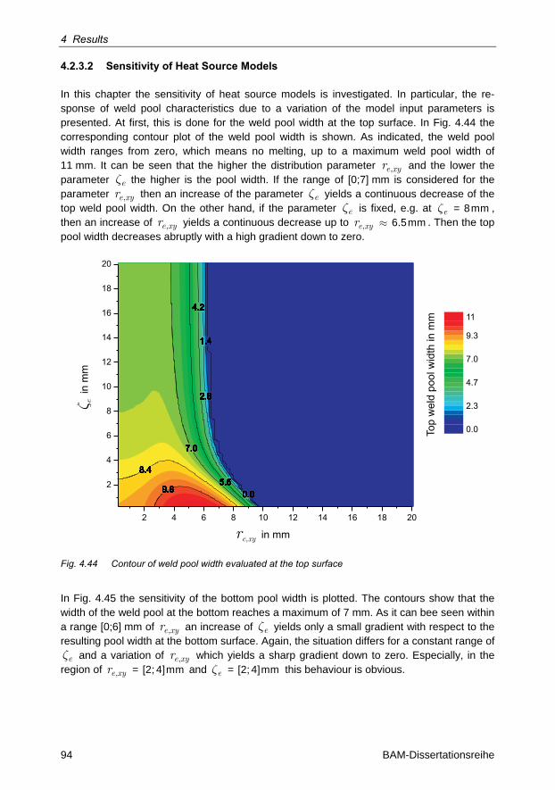
4 Results
94 BAM-Dissertationsreihe
4.2.3.2 Sensitivity of Heat Source Models
In this chapter the sensitivity of heat source models is investigated. In particular, the re-sponse of weld pool characteristics due to a variation of the model input parameters is presented. At first, this is done for the weld pool width at the top surface. In Fig. 4.44 the corresponding contour plot of the weld pool width is shown. As indicated, the weld pool width ranges from zero, which means no melting, up to a maximum weld pool width of 11 mm. It can be seen that the higher the distribution parameter e xyr , and the lower the parameter ez the higher is the pool width. If the range of [0;7] mm is considered for the parameter e xyr , then an increase of the parameter ez yields a continuous decrease of the top weld pool width. On the other hand, if the parameter ez is fixed, e.g. at ez = 8mm , then an increase of e xyr , yields a continuous decrease up to e xyr , » 6.5mm . Then the top pool width decreases abruptly with a high gradient down to zero.
Top
wel
d po
ol w
idth
in m
m
9.8
8.4
7.0
5.6
4.2
2.8
1.4
0.09.8
8.4
7.0
5.6
4.2
2.8
1.4
0.09.8
8.4
7.0
5.6
4.2
2.8
1.4
0.09.8
8.4
7.0
5.6
4.2
2.8
1.4
0.09.8
8.4
7.0
5.6
4.2
2.8
1.4
0.09.8
8.4
7.0
5.6
4.2
2.8
1.4
0.09.8
8.4
7.0
5.6
4.2
2.8
1.4
0.09.8
8.4
7.0
5.6
4.2
2.8
1.4
0.09.8
8.4
7.0
5.6
4.2
2.8
1.4
0.09.8
8.4
7.0
5.6
4.2
2.8
1.4
0.09.8
8.4
7.0
5.6
4.2
2.8
1.4
0.09.8
8.4
7.0
5.6
4.2
2.8
1.4
0.09.8
8.4
7.0
5.6
4.2
2.8
1.4
0.09.8
8.4
7.0
5.6
4.2
2.8
1.4
0.09.8
8.4
7.0
5.6
4.2
2.8
1.4
0.09.8
8.4
7.0
5.6
4.2
2.8
1.4
0.09.8
8.4
7.0
5.6
4.2
2.8
1.4
0.09.8
8.4
7.0
5.6
4.2
2.8
1.4
0.09.8
8.4
7.0
5.6
4.2
2.8
1.4
0.09.8
8.4
7.0
5.6
4.2
2.8
1.4
0.09.8
8.4
7.0
5.6
4.2
2.8
1.4
0.09.8
8.4
7.0
5.6
4.2
2.8
1.4
0.09.8
8.4
7.0
5.6
4.2
2.8
1.4
0.09.8
8.4
7.0
5.6
4.2
2.8
1.4
0.09.8
8.4
7.0
5.6
4.2
2.8
1.4
0.09.8
8.4
7.0
5.6
4.2
2.8
1.4
0.09.8
8.4
7.0
5.6
4.2
2.8
1.4
0.09.8
8.4
7.0
5.6
4.2
2.8
1.4
0.09.8
8.4
7.0
5.6
4.2
2.8
1.4
0.09.8
8.4
7.0
5.6
4.2
2.8
1.4
0.09.8
8.4
7.0
5.6
4.2
2.8
1.4
0.09.8
8.4
7.0
5.6
4.2
2.8
1.4
0.09.8
8.4
7.0
5.6
4.2
2.8
1.4
0.09.8
8.4
7.0
5.6
4.2
2.8
1.4
0.09.8
8.4
7.0
5.6
4.2
2.8
1.4
0.09.8
8.4
7.0
5.6
4.2
2.8
1.4
0.09.8
8.4
7.0
5.6
4.2
2.8
1.4
0.09.8
8.4
7.0
5.6
4.2
2.8
1.4
0.09.8
8.4
7.0
5.6
4.2
2.8
1.4
0.09.8
8.4
7.0
5.6
4.2
2.8
1.4
0.09.8
8.4
7.0
5.6
4.2
2.8
1.4
0.09.8
8.4
7.0
5.6
4.2
2.8
1.4
0.09.8
8.4
7.0
5.6
4.2
2.8
1.4
0.09.8
8.4
7.0
5.6
4.2
2.8
1.4
0.09.8
8.4
7.0
5.6
4.2
2.8
1.4
0.09.8
8.4
7.0
5.6
4.2
2.8
1.4
0.09.8
8.4
7.0
5.6
4.2
2.8
1.4
0.09.8
8.4
7.0
5.6
4.2
2.8
1.4
0.09.8
8.4
7.0
5.6
4.2
2.8
1.4
0.09.8
8.4
7.0
5.6
4.2
2.8
1.4
0.09.8
8.4
7.0
5.6
4.2
2.8
1.4
0.0
2 4 6 8 10 12 14 16 18 20
2
4
6
8
10
12
14
16
18
20
0.0
2.3
4.7
7.0
9.3
11
re,xy in mm
� ein
mm
Fig. 4.44 Contour of weld pool width evaluated at the top surface
In Fig. 4.45 the sensitivity of the bottom pool width is plotted. The contours show that the width of the weld pool at the bottom reaches a maximum of 7 mm. As it can bee seen within a range [0;6] mm of e xyr , an increase of ez yields only a small gradient with respect to the resulting pool width at the bottom surface. Again, the situation differs for a constant range of
ez and a variation of e xyr , which yields a sharp gradient down to zero. Especially, in the region of e xyr , = [2; 4]mm and ez = [2; 4]mm this behaviour is obvious.
4.2 Computational Investigations
95
Bot
tom
wel
d po
ol w
idth
in m
m
6.2
5.3
4.4
3.5
2.6
1.8
0.88
0.0
6.2
5.3
4.4
3.5
2.6
1.8
0.88
0.0
6.2
5.3
4.4
3.5
2.6
1.8
0.88
0.0
6.2
5.3
4.4
3.5
2.6
1.8
0.88
0.0
6.2
5.3
4.4
3.5
2.6
1.8
0.88
0.0
6.2
5.3
4.4
3.5
2.6
1.8
0.88
0.0
6.2
5.3
4.4
3.5
2.6
1.8
0.88
0.0
6.2
5.3
4.4
3.5
2.6
1.8
0.88
0.0
6.2
5.3
4.4
3.5
2.6
1.8
0.88
0.0
6.2
5.3
4.4
3.5
2.6
1.8
0.88
0.0
6.2
5.3
4.4
3.5
2.6
1.8
0.88
0.0
6.2
5.3
4.4
3.5
2.6
1.8
0.88
0.0
6.2
5.3
4.4
3.5
2.6
1.8
0.88
0.0
6.2
5.3
4.4
3.5
2.6
1.8
0.88
0.0
6.2
5.3
4.4
3.5
2.6
1.8
0.88
0.0
6.2
5.3
4.4
3.5
2.6
1.8
0.88
0.0
6.2
5.3
4.4
3.5
2.6
1.8
0.88
0.0
6.2
5.3
4.4
3.5
2.6
1.8
0.88
0.0
6.2
5.3
4.4
3.5
2.6
1.8
0.88
0.0
6.2
5.3
4.4
3.5
2.6
1.8
0.88
0.0
6.2
5.3
4.4
3.5
2.6
1.8
0.88
0.0
6.2
5.3
4.4
3.5
2.6
1.8
0.88
0.0
6.2
5.3
4.4
3.5
2.6
1.8
0.88
0.0
6.2
5.3
4.4
3.5
2.6
1.8
0.88
0.0
6.2
5.3
4.4
3.5
2.6
1.8
0.88
0.0
6.2
5.3
4.4
3.5
2.6
1.8
0.88
0.0
6.2
5.3
4.4
3.5
2.6
1.8
0.88
0.0
6.2
5.3
4.4
3.5
2.6
1.8
0.88
0.0
6.2
5.3
4.4
3.5
2.6
1.8
0.88
0.0
6.2
5.3
4.4
3.5
2.6
1.8
0.88
0.0
6.2
5.3
4.4
3.5
2.6
1.8
0.88
0.0
6.2
5.3
4.4
3.5
2.6
1.8
0.88
0.0
6.2
5.3
4.4
3.5
2.6
1.8
0.88
0.0
6.2
5.3
4.4
3.5
2.6
1.8
0.88
0.0
6.2
5.3
4.4
3.5
2.6
1.8
0.88
0.0
6.2
5.3
4.4
3.5
2.6
1.8
0.88
0.0
6.2
5.3
4.4
3.5
2.6
1.8
0.88
0.0
6.2
5.3
4.4
3.5
2.6
1.8
0.88
0.0
6.2
5.3
4.4
3.5
2.6
1.8
0.88
0.0
6.2
5.3
4.4
3.5
2.6
1.8
0.88
0.0
6.2
5.3
4.4
3.5
2.6
1.8
0.88
0.0
6.2
5.3
4.4
3.5
2.6
1.8
0.88
0.0
6.2
5.3
4.4
3.5
2.6
1.8
0.88
0.0
6.2
5.3
4.4
3.5
2.6
1.8
0.88
0.0
6.2
5.3
4.4
3.5
2.6
1.8
0.88
0.0
6.2
5.3
4.4
3.5
2.6
1.8
0.88
0.0
6.2
5.3
4.4
3.5
2.6
1.8
0.88
0.0
6.2
5.3
4.4
3.5
2.6
1.8
0.88
0.0
6.2
5.3
4.4
3.5
2.6
1.8
0.88
0.0
6.2
5.3
4.4
3.5
2.6
1.8
0.88
0.0
6.2
5.3
4.4
3.5
2.6
1.8
0.88
0.0
2 4 6 8 10 12 14 16 18 20
2
4
6
8
10
12
14
16
18
20
0.0
1.5
2.9
4.4
5.9
7.0
re,xy in mm
� ein
mm
Fig. 4.45 Contour of weld pool width evaluated at the bottom surface
In Fig. 4.46 the contour of the weld pool depth is illustrated. The maximum is truncated at 6 mm that corresponds to the thickness of the plate under consideration. It can be seen that the range of penetration becomes more and more narrow if the parameter ez increases. The same is true for the parameter e xyr , . Again, a high gradient downwards no melting occurs especially for great values of ez .
Fig. 4.47 shows the contour of the weld pool length that is evaluated at the top surface. Within the range of model parameters a maximum weld pool length of 18 mm can be ob-tained. Again, a high gradient downwards no melting occurs in direction of increasing val-ues of e xyr , . It is interesting to note that if ez is greater than 8 mm no gradient in direction of increasing values of ez can be obtained.
To summarize it can be said that for all investigated weld pool characteristics the gradient in direction of e xyr , is significantly greater than in direction of ez . Furthermore, if e xyr , is greater than 9.5 mm no melting occurs independently on the values of ez .
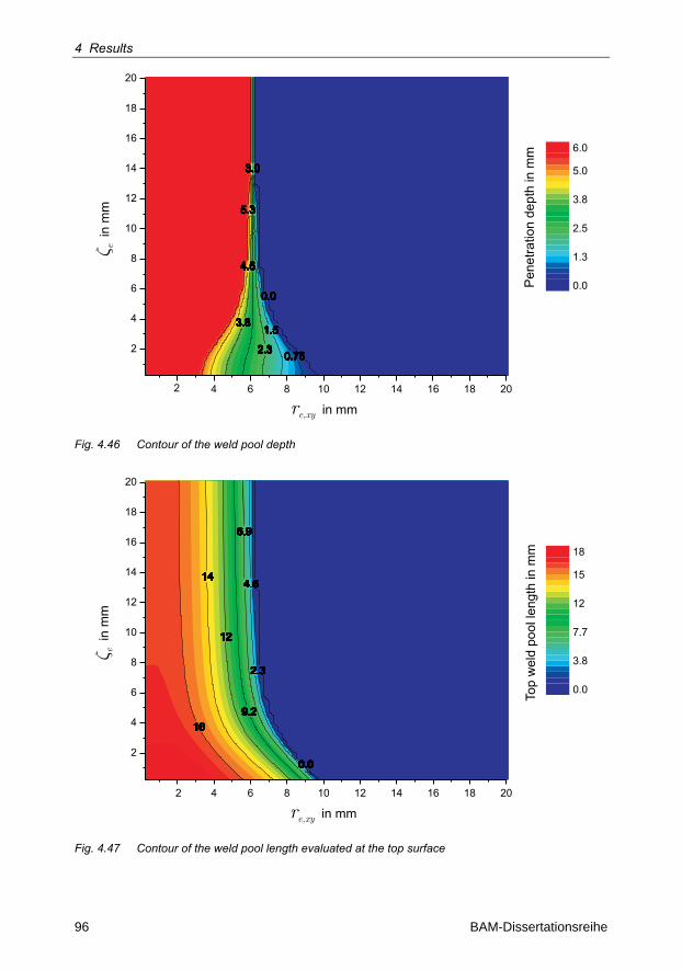
4 Results
96 BAM-Dissertationsreihe
Pen
etra
tion
dept
h in
mm
5.3
4.5
3.8
3.0
2.3
1.5
0.75
0.0
5.3
4.5
3.8
3.0
2.3
1.5
0.75
0.0
5.3
4.5
3.8
3.0
2.3
1.5
0.75
0.0
5.3
4.5
3.8
3.0
2.3
1.5
0.75
0.0
5.3
4.5
3.8
3.0
2.3
1.5
0.75
0.0
5.3
4.5
3.8
3.0
2.3
1.5
0.75
0.0
5.3
4.5
3.8
3.0
2.3
1.5
0.75
0.0
5.3
4.5
3.8
3.0
2.3
1.5
0.75
0.0
5.3
4.5
3.8
3.0
2.3
1.5
0.75
0.0
5.3
4.5
3.8
3.0
2.3
1.5
0.75
0.0
5.3
4.5
3.8
3.0
2.3
1.5
0.75
0.0
5.3
4.5
3.8
3.0
2.3
1.5
0.75
0.0
5.3
4.5
3.8
3.0
2.3
1.5
0.75
0.0
5.3
4.5
3.8
3.0
2.3
1.5
0.75
0.0
5.3
4.5
3.8
3.0
2.3
1.5
0.75
0.0
5.3
4.5
3.8
3.0
2.3
1.5
0.75
0.0
5.3
4.5
3.8
3.0
2.3
1.5
0.75
0.0
5.3
4.5
3.8
3.0
2.3
1.5
0.75
0.0
5.3
4.5
3.8
3.0
2.3
1.5
0.75
0.0
5.3
4.5
3.8
3.0
2.3
1.5
0.75
0.0
5.3
4.5
3.8
3.0
2.3
1.5
0.75
0.0
5.3
4.5
3.8
3.0
2.3
1.5
0.75
0.0
5.3
4.5
3.8
3.0
2.3
1.5
0.75
0.0
5.3
4.5
3.8
3.0
2.3
1.5
0.75
0.0
5.3
4.5
3.8
3.0
2.3
1.5
0.75
0.0
5.3
4.5
3.8
3.0
2.3
1.5
0.75
0.0
5.3
4.5
3.8
3.0
2.3
1.5
0.75
0.0
5.3
4.5
3.8
3.0
2.3
1.5
0.75
0.0
5.3
4.5
3.8
3.0
2.3
1.5
0.75
0.0
5.3
4.5
3.8
3.0
2.3
1.5
0.75
0.0
5.3
4.5
3.8
3.0
2.3
1.5
0.75
0.0
5.3
4.5
3.8
3.0
2.3
1.5
0.75
0.0
5.3
4.5
3.8
3.0
2.3
1.5
0.75
0.0
5.3
4.5
3.8
3.0
2.3
1.5
0.75
0.0
5.3
4.5
3.8
3.0
2.3
1.5
0.75
0.0
5.3
4.5
3.8
3.0
2.3
1.5
0.75
0.0
5.3
4.5
3.8
3.0
2.3
1.5
0.75
0.0
5.3
4.5
3.8
3.0
2.3
1.5
0.75
0.0
5.3
4.5
3.8
3.0
2.3
1.5
0.75
0.0
5.3
4.5
3.8
3.0
2.3
1.5
0.75
0.0
5.3
4.5
3.8
3.0
2.3
1.5
0.75
0.0
5.3
4.5
3.8
3.0
2.3
1.5
0.75
0.0
5.3
4.5
3.8
3.0
2.3
1.5
0.75
0.0
5.3
4.5
3.8
3.0
2.3
1.5
0.75
0.0
5.3
4.5
3.8
3.0
2.3
1.5
0.75
0.0
5.3
4.5
3.8
3.0
2.3
1.5
0.75
0.0
5.3
4.5
3.8
3.0
2.3
1.5
0.75
0.0
5.3
4.5
3.8
3.0
2.3
1.5
0.75
0.0
5.3
4.5
3.8
3.0
2.3
1.5
0.75
0.0
2 4 6 8 10 12 14 16 18 20
2
4
6
8
10
12
14
16
18
20
0.0
1.3
2.5
3.8
5.0
6.0
re,xy in mm
� ein
mm
Fig. 4.46 Contour of the weld pool depth
Top
wel
d po
ol le
ngth
in m
m
16
14
12
9.2
6.9
4.6
2.3
0.0
16
14
12
9.2
6.9
4.6
2.3
0.0
16
14
12
9.2
6.9
4.6
2.3
0.0
16
14
12
9.2
6.9
4.6
2.3
0.0
16
14
12
9.2
6.9
4.6
2.3
0.0
16
14
12
9.2
6.9
4.6
2.3
0.0
16
14
12
9.2
6.9
4.6
2.3
0.0
16
14
12
9.2
6.9
4.6
2.3
0.0
16
14
12
9.2
6.9
4.6
2.3
0.0
16
14
12
9.2
6.9
4.6
2.3
0.0
16
14
12
9.2
6.9
4.6
2.3
0.0
16
14
12
9.2
6.9
4.6
2.3
0.0
16
14
12
9.2
6.9
4.6
2.3
0.0
16
14
12
9.2
6.9
4.6
2.3
0.0
16
14
12
9.2
6.9
4.6
2.3
0.0
16
14
12
9.2
6.9
4.6
2.3
0.0
16
14
12
9.2
6.9
4.6
2.3
0.0
16
14
12
9.2
6.9
4.6
2.3
0.0
16
14
12
9.2
6.9
4.6
2.3
0.0
16
14
12
9.2
6.9
4.6
2.3
0.0
16
14
12
9.2
6.9
4.6
2.3
0.0
16
14
12
9.2
6.9
4.6
2.3
0.0
16
14
12
9.2
6.9
4.6
2.3
0.0
16
14
12
9.2
6.9
4.6
2.3
0.0
16
14
12
9.2
6.9
4.6
2.3
0.0
16
14
12
9.2
6.9
4.6
2.3
0.0
16
14
12
9.2
6.9
4.6
2.3
0.0
16
14
12
9.2
6.9
4.6
2.3
0.0
16
14
12
9.2
6.9
4.6
2.3
0.0
16
14
12
9.2
6.9
4.6
2.3
0.0
16
14
12
9.2
6.9
4.6
2.3
0.0
16
14
12
9.2
6.9
4.6
2.3
0.0
16
14
12
9.2
6.9
4.6
2.3
0.0
16
14
12
9.2
6.9
4.6
2.3
0.0
16
14
12
9.2
6.9
4.6
2.3
0.0
16
14
12
9.2
6.9
4.6
2.3
0.0
16
14
12
9.2
6.9
4.6
2.3
0.0
16
14
12
9.2
6.9
4.6
2.3
0.0
16
14
12
9.2
6.9
4.6
2.3
0.0
16
14
12
9.2
6.9
4.6
2.3
0.0
16
14
12
9.2
6.9
4.6
2.3
0.0
16
14
12
9.2
6.9
4.6
2.3
0.0
16
14
12
9.2
6.9
4.6
2.3
0.0
16
14
12
9.2
6.9
4.6
2.3
0.0
16
14
12
9.2
6.9
4.6
2.3
0.0
16
14
12
9.2
6.9
4.6
2.3
0.0
16
14
12
9.2
6.9
4.6
2.3
0.0
16
14
12
9.2
6.9
4.6
2.3
0.0
16
14
12
9.2
6.9
4.6
2.3
0.0
16
14
12
9.2
6.9
4.6
2.3
0.0
16
14
12
9.2
6.9
4.6
2.3
0.0
2 4 6 8 10 12 14 16 18 20
2
4
6
8
10
12
14
16
18
20
0.0
3.8
7.7
12
15
18
re,xy in mm
� ein
mm
Fig. 4.47 Contour of the weld pool length evaluated at the top surface
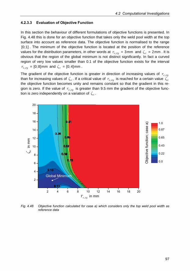
4.2 Computational Investigations
97
4.2.3.3 Evaluation of Objective Function
In this section the behaviour of different formulations of objective functions is presented. In Fig. 4.48 this is done for an objective function that takes only the weld pool width at the top surface into account as reference data. The objective function is normalised to the range [0;1] . The minimum of the objective function is located at the position of the reference values for the distribution parameters, in other words at e xyr , = 3mm and ez = 2mm . It is obvious that the region of the global minimum is not distinct significantly. In fact a curved region of very low values smaller than 0.1 of the objective function exists for the interval
e xyr , = [0;8]mm and ez = [0; 4]mm .
The gradient of the objective function is greater in direction of increasing values of e xyr , than for increasing values of ez . If a critical value of e xyr , is reached for a certain value ez the objective function becomes unity and remains constant so that the gradient in this re-gion is zero. If the value of e xyr , is greater than 9.5 mm the gradient of the objective func-tion is zero independently on a variation of ez .
0.13
0.130.130.130.130.130.130.130.130.130.130.130.130.130.130.130.130.130.130.130.130.130.130.130.130.130.130.130.13
0.260.260.260.260.260.260.260.260.260.260.260.260.260.260.260.260.260.260.260.260.260.260.260.260.260.260.260.26
0.390.390.390.390.390.390.390.390.390.390.390.390.390.390.390.390.390.390.390.390.390.390.390.390.390.390.390.39
0.520.520.520.520.520.520.520.520.520.520.520.520.520.520.520.520.520.520.520.520.520.520.520.520.520.520.520.52
0.650.650.650.650.650.650.650.650.650.650.650.650.650.650.650.650.650.650.650.650.650.650.650.650.650.650.650.65
0.780.780.780.780.780.780.780.780.780.780.780.780.780.780.780.780.780.780.780.780.780.780.780.780.780.780.780.78
0.910.910.910.910.910.910.910.910.910.910.910.910.910.910.910.910.910.910.910.910.910.910.910.910.910.910.910.910.91
0.78
0.65
0.52
0.39
0.26
0.13
0.13
0.130.130.130.130.130.130.130.130.130.130.130.130.130.130.130.130.130.130.130.130.130.130.130.130.130.130.130.13
0.260.260.260.260.260.260.260.260.260.260.260.260.260.260.260.260.260.260.260.260.260.260.260.260.260.260.260.26
0.390.390.390.390.390.390.390.390.390.390.390.390.390.390.390.390.390.390.390.390.390.390.390.390.390.390.390.39
0.520.520.520.520.520.520.520.520.520.520.520.520.520.520.520.520.520.520.520.520.520.520.520.520.520.520.520.52
0.650.650.650.650.650.650.650.650.650.650.650.650.650.650.650.650.650.650.650.650.650.650.650.650.650.650.650.65
0.780.780.780.780.780.780.780.780.780.780.780.780.780.780.780.780.780.780.780.780.780.780.780.780.780.780.780.78
0.910.910.910.910.910.910.910.910.910.910.910.910.910.910.910.910.910.910.910.910.910.910.910.910.910.910.910.910.91
0.78
0.65
0.52
0.39
0.26
0.13
2 4 6 8 10 12 14 16 18 20
2
4
6
8
10
12
14
16
18
20
0.0
0.22
0.43
0.65
0.87
1.0
Obj
ectiv
e fu
nctio
n; c
ase
a)
Global Minimum
re,xy in mm
� ein
mm
Fig. 4.48 Objective function calculated for case a) which considers only the top weld pool width as reference data
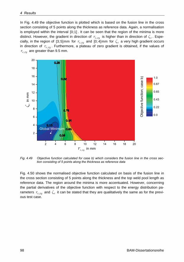
4 Results
98 BAM-Dissertationsreihe
In Fig. 4.49 the objective function is plotted which is based on the fusion line in the cross section consisting of 5 points along the thickness as reference data. Again, a normalisation is employed within the interval [0;1] . It can be seen that the region of the minima is more distinct. However, the gradient in direction of e xyr , is higher than in direction of ez . Espe-cially, in the region of [3;5]mm for e xyr , and [0; 4]mm for ez a very high gradient occurs in direction of e xyr , . Furthermore, a plateau of zero gradient is obtained, if the values of
e xyr , are greater than 9.5 mm.
0.130.130.13
0.260.260.26
0.390.390.39
0.520.520.52
0.650.650.65
0.780.780.78
0.910.910.910.91
0.78
0.65
0.52
0.39
0.26
0.130.130.130.13
0.260.260.26
0.390.390.39
0.520.520.52
0.650.650.65
0.780.780.78
0.910.910.910.91
0.78
0.65
0.52
0.39
0.26
0.130.130.130.13
0.260.260.26
0.390.390.39
0.520.520.52
0.650.650.65
0.780.780.78
0.910.910.910.91
0.78
0.65
0.52
0.39
0.26
0.130.130.130.13
0.260.260.26
0.390.390.39
0.520.520.52
0.650.650.65
0.780.780.78
0.910.910.910.91
0.78
0.65
0.52
0.39
0.26
0.130.130.130.13
0.260.260.26
0.390.390.39
0.520.520.52
0.650.650.65
0.780.780.78
0.910.910.910.91
0.78
0.65
0.52
0.39
0.26
0.130.130.130.13
0.260.260.26
0.390.390.39
0.520.520.52
0.650.650.65
0.780.780.78
0.910.910.910.91
0.78
0.65
0.52
0.39
0.26
0.130.130.130.13
0.260.260.26
0.390.390.39
0.520.520.52
0.650.650.65
0.780.780.78
0.910.910.910.91
0.78
0.65
0.52
0.39
0.26
0.130.130.130.13
0.260.260.26
0.390.390.39
0.520.520.52
0.650.650.65
0.780.780.78
0.910.910.910.91
0.78
0.65
0.52
0.39
0.26
0.130.130.130.13
0.260.260.26
0.390.390.39
0.520.520.52
0.650.650.65
0.780.780.78
0.910.910.910.91
0.78
0.65
0.52
0.39
0.26
0.130.130.130.13
0.260.260.26
0.390.390.39
0.520.520.52
0.650.650.65
0.780.780.78
0.910.910.910.91
0.78
0.65
0.52
0.39
0.26
0.130.130.130.13
0.260.260.26
0.390.390.39
0.520.520.52
0.650.650.65
0.780.780.78
0.910.910.910.91
0.78
0.65
0.52
0.39
0.26
0.130.130.130.13
0.260.260.26
0.390.390.39
0.520.520.52
0.650.650.65
0.780.780.78
0.910.910.910.91
0.78
0.65
0.52
0.39
0.26
0.130.130.130.13
0.260.260.26
0.390.390.39
0.520.520.52
0.650.650.65
0.780.780.78
0.910.910.910.91
0.78
0.65
0.52
0.39
0.26
0.130.130.130.13
0.260.260.26
0.390.390.39
0.520.520.52
0.650.650.65
0.780.780.78
0.910.910.910.91
0.78
0.65
0.52
0.39
0.26
0.130.130.130.13
0.260.260.26
0.390.390.39
0.520.520.52
0.650.650.65
0.780.780.78
0.910.910.910.91
0.78
0.65
0.52
0.39
0.26
0.130.130.130.13
0.260.260.26
0.390.390.39
0.520.520.52
0.650.650.65
0.780.780.78
0.910.910.910.91
0.78
0.65
0.52
0.39
0.26
0.130.130.130.13
0.260.260.26
0.390.390.39
0.520.520.52
0.650.650.65
0.780.780.78
0.910.910.910.91
0.78
0.65
0.52
0.39
0.26
0.130.130.130.13
0.260.260.26
0.390.390.39
0.520.520.52
0.650.650.65
0.780.780.78
0.910.910.910.91
0.78
0.65
0.52
0.39
0.26
0.130.130.130.13
0.260.260.26
0.390.390.39
0.520.520.52
0.650.650.65
0.780.780.78
0.910.910.910.91
0.78
0.65
0.52
0.39
0.26
0.130.130.130.13
0.260.260.26
0.390.390.39
0.520.520.52
0.650.650.65
0.780.780.78
0.910.910.910.91
0.78
0.65
0.52
0.39
0.26
0.130.130.130.13
0.260.260.26
0.390.390.39
0.520.520.52
0.650.650.65
0.780.780.78
0.910.910.910.91
0.78
0.65
0.52
0.39
0.26
0.130.130.130.13
0.260.260.26
0.390.390.39
0.520.520.52
0.650.650.65
0.780.780.78
0.910.910.910.91
0.78
0.65
0.52
0.39
0.26
0.130.130.130.13
0.260.260.26
0.390.390.39
0.520.520.52
0.650.650.65
0.780.780.78
0.910.910.910.91
0.78
0.65
0.52
0.39
0.26
0.130.130.130.13
0.260.260.26
0.390.390.39
0.520.520.52
0.650.650.65
0.780.780.78
0.910.910.910.91
0.78
0.65
0.52
0.39
0.26
0.130.130.130.13
0.260.260.26
0.390.390.39
0.520.520.52
0.650.650.65
0.780.780.78
0.910.910.910.91
0.78
0.65
0.52
0.39
0.26
0.130.130.130.13
0.260.260.26
0.390.390.39
0.520.520.52
0.650.650.65
0.780.780.78
0.910.910.910.91
0.78
0.65
0.52
0.39
0.26
0.130.130.130.13
0.260.260.26
0.390.390.39
0.520.520.52
0.650.650.65
0.780.780.78
0.910.910.910.91
0.78
0.65
0.52
0.39
0.26
0.130.130.130.13
0.260.260.26
0.390.390.39
0.520.520.52
0.650.650.65
0.780.780.78
0.910.910.910.91
0.78
0.65
0.52
0.39
0.26
0.130.130.130.13
0.260.260.26
0.390.390.39
0.520.520.52
0.650.650.65
0.780.780.78
0.910.910.910.91
0.78
0.65
0.52
0.39
0.26
0.130.130.130.13
0.260.260.26
0.390.390.39
0.520.520.52
0.650.650.65
0.780.780.78
0.910.910.910.91
0.78
0.65
0.52
0.39
0.26
0.130.130.130.13
0.260.260.26
0.390.390.39
0.520.520.52
0.650.650.65
0.780.780.78
0.910.910.910.91
0.78
0.65
0.52
0.39
0.26
0.130.130.130.13
0.260.260.26
0.390.390.39
0.520.520.52
0.650.650.65
0.780.780.78
0.910.910.910.91
0.78
0.65
0.52
0.39
0.26
0.130.130.130.13
0.260.260.26
0.390.390.39
0.520.520.52
0.650.650.65
0.780.780.78
0.910.910.910.91
0.78
0.65
0.52
0.39
0.26
0.130.130.130.13
0.260.260.26
0.390.390.39
0.520.520.52
0.650.650.65
0.780.780.78
0.910.910.910.91
0.78
0.65
0.52
0.39
0.26
0.130.130.130.13
0.260.260.26
0.390.390.39
0.520.520.52
0.650.650.65
0.780.780.78
0.910.910.910.91
0.78
0.65
0.52
0.39
0.26
0.130.130.130.13
0.260.260.26
0.390.390.39
0.520.520.52
0.650.650.65
0.780.780.78
0.910.910.910.91
0.78
0.65
0.52
0.39
0.26
0.130.130.130.13
0.260.260.26
0.390.390.39
0.520.520.52
0.650.650.65
0.780.780.78
0.910.910.910.91
0.78
0.65
0.52
0.39
0.26
0.130.130.130.13
0.260.260.26
0.390.390.39
0.520.520.52
0.650.650.65
0.780.780.78
0.910.910.910.91
0.78
0.65
0.52
0.39
0.26
0.130.130.130.13
0.260.260.26
0.390.390.39
0.520.520.52
0.650.650.65
0.780.780.78
0.910.910.910.91
0.78
0.65
0.52
0.39
0.26
0.130.130.130.13
0.260.260.26
0.390.390.39
0.520.520.52
0.650.650.65
0.780.780.78
0.910.910.910.91
0.78
0.65
0.52
0.39
0.26
0.130.130.130.13
0.260.260.26
0.390.390.39
0.520.520.52
0.650.650.65
0.780.780.78
0.910.910.910.91
0.78
0.65
0.52
0.39
0.26
0.130.130.130.13
0.260.260.26
0.390.390.39
0.520.520.52
0.650.650.65
0.780.780.78
0.910.910.910.91
0.78
0.65
0.52
0.39
0.26
0.130.130.130.13
0.260.260.26
0.390.390.39
0.520.520.52
0.650.650.65
0.780.780.78
0.910.910.910.91
0.78
0.65
0.52
0.39
0.26
0.130.130.130.13
0.260.260.26
0.390.390.39
0.520.520.52
0.650.650.65
0.780.780.78
0.910.910.910.91
0.78
0.65
0.52
0.39
0.26
0.130.130.130.13
0.260.260.26
0.390.390.39
0.520.520.52
0.650.650.65
0.780.780.78
0.910.910.910.91
0.78
0.65
0.52
0.39
0.26
0.130.130.130.13
0.260.260.26
0.390.390.39
0.520.520.52
0.650.650.65
0.780.780.78
0.910.910.910.91
0.78
0.65
0.52
0.39
0.26
0.130.130.130.13
0.260.260.26
0.390.390.39
0.520.520.52
0.650.650.65
0.780.780.78
0.910.910.910.91
0.78
0.65
0.52
0.39
0.26
0.13
2 4 6 8 10 12 14 16 18 20
2
4
6
8
10
12
14
16
18
20
0.0
0.22
0.43
0.65
0.87
1.0
Obj
ectiv
e fu
nctio
n; c
ase
b)
re,xy in mm
� ein
mm
Global Minimum
Fig. 4.49 Objective function calculated for case b) which considers the fusion line in the cross sec-tion consisting of 5 points along the thickness as reference data
Fig. 4.50 shows the normalised objective function calculated on basis of the fusion line in the cross section consisting of 5 points along the thickness and the top weld pool length as reference data. The region around the minima is more accentuated. However, concerning the partial derivatives of the objective function with respect to the energy distribution pa-rameters e xyr , and ez it can be stated that they are qualitatively the same as for the previ-ous test case.
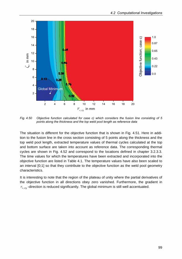
4.2 Computational Investigations
99
0.130.130.130.130.130.130.130.130.130.13 0.260.260.260.260.260.260.260.260.260.26
0.390.390.390.390.390.390.390.390.390.39
0.520.520.520.520.520.520.520.520.520.52
0.650.650.650.650.650.650.650.650.650.65
0.780.780.780.780.780.780.780.780.780.78
0.910.910.910.910.910.910.910.910.910.910.91
0.78
0.65
0.52
0.39
0.260.130.130.130.130.130.130.130.130.130.130.13 0.260.260.260.260.260.260.260.260.260.26
0.390.390.390.390.390.390.390.390.390.39
0.520.520.520.520.520.520.520.520.520.52
0.650.650.650.650.650.650.650.650.650.65
0.780.780.780.780.780.780.780.780.780.78
0.910.910.910.910.910.910.910.910.910.910.91
0.78
0.65
0.52
0.39
0.260.13
2 4 6 8 10 12 14 16 18 20
2
4
6
8
10
12
14
16
18
20
0.0
0.22
0.43
0.65
0.87
1.0
Obj
ectiv
e fu
nctio
n; c
ase
c)
re,xy in mm
� ein
mm
Global Minimum
Fig. 4.50 Objective function calculated for case c) which considers the fusion line consisting of 5 points along the thickness and the top weld pool length as reference data
The situation is different for the objective function that is shown in Fig. 4.51. Here in addi-tion to the fusion line in the cross section consisting of 5 points along the thickness and the top weld pool length, extracted temperature values of thermal cycles calculated at the top and bottom surface are taken into account as reference data. The corresponding thermal cycles are shown in Fig. 4.52 and correspond to the locations defined in chapter 3.2.3.3. The time values for which the temperatures have been extracted and incorporated into the objective function are listed in Table 4.1. The temperature values have also been scaled to an interval [0;1] so that they contribute to the objective function as the weld pool geometry characteristics.
It is interesting to note that the region of the plateau of unity where the partial derivatives of the objective function in all directions obey zero vanished. Furthermore, the gradient in
e xyr , -direction is reduced significantly. The global minimum is still well accentuated.
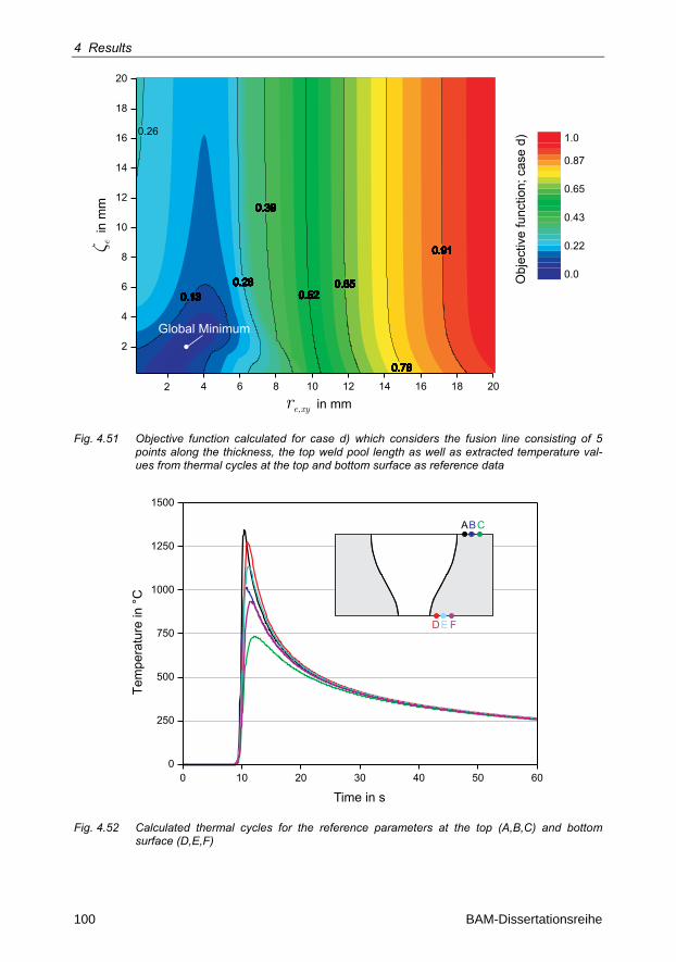
4 Results
100 BAM-Dissertationsreihe
0.130.130.13
0.91
0.260.260.26
0.78
0.390.390.39
0.650.520.520.520.52
0.39
0.260.130.130.130.13
0.91
0.260.260.26
0.78
0.390.390.39
0.650.520.520.520.52
0.39
0.260.130.130.130.13
0.91
0.260.260.26
0.78
0.390.390.39
0.650.520.520.520.52
0.39
0.260.130.130.130.13
0.91
0.260.260.26
0.78
0.390.390.39
0.650.520.520.520.52
0.39
0.260.130.130.130.13
0.91
0.260.260.26
0.78
0.390.390.39
0.650.520.520.520.52
0.39
0.260.130.130.130.13
0.91
0.260.260.26
0.78
0.390.390.39
0.650.520.520.520.52
0.39
0.260.130.130.130.13
0.91
0.260.260.26
0.78
0.390.390.39
0.650.520.520.520.52
0.39
0.260.130.130.130.13
0.91
0.260.260.26
0.78
0.390.390.39
0.650.520.520.520.52
0.39
0.260.130.130.130.13
0.91
0.260.260.26
0.78
0.390.390.39
0.650.520.520.520.52
0.39
0.260.130.130.130.13
0.91
0.260.260.26
0.78
0.390.390.39
0.650.520.520.520.52
0.39
0.260.130.130.130.13
0.91
0.260.260.26
0.78
0.390.390.39
0.650.520.520.520.52
0.39
0.260.130.130.130.13
0.91
0.260.260.26
0.78
0.390.390.39
0.650.520.520.520.52
0.39
0.260.130.130.130.13
0.91
0.260.260.26
0.78
0.390.390.39
0.650.520.520.520.52
0.39
0.260.130.130.130.13
0.91
0.260.260.26
0.78
0.390.390.39
0.650.520.520.520.52
0.39
0.260.130.130.130.13
0.91
0.260.260.26
0.78
0.390.390.39
0.650.520.520.520.52
0.39
0.260.130.130.130.13
0.91
0.260.260.26
0.78
0.390.390.39
0.650.520.520.520.52
0.39
0.260.130.130.130.13
0.91
0.260.260.26
0.78
0.390.390.39
0.650.520.520.520.52
0.39
0.260.130.130.130.13
0.91
0.260.260.26
0.78
0.390.390.39
0.650.520.520.520.52
0.39
0.260.130.130.130.13
0.91
0.260.260.26
0.78
0.390.390.39
0.650.520.520.520.52
0.39
0.260.130.130.130.13
0.91
0.260.260.26
0.78
0.390.390.39
0.650.520.520.520.52
0.39
0.260.130.130.130.13
0.91
0.260.260.26
0.78
0.390.390.39
0.650.520.520.520.52
0.39
0.260.130.130.130.13
0.91
0.260.260.26
0.78
0.390.390.39
0.650.520.520.520.52
0.39
0.260.130.130.130.13
0.91
0.260.260.26
0.78
0.390.390.39
0.650.520.520.520.52
0.39
0.260.130.130.130.13
0.91
0.260.260.26
0.78
0.390.390.39
0.650.520.520.520.52
0.39
0.260.130.130.130.13
0.91
0.260.260.26
0.78
0.390.390.39
0.650.520.520.520.52
0.39
0.260.130.130.130.13
0.91
0.260.260.26
0.78
0.390.390.39
0.650.520.520.520.52
0.39
0.260.130.130.130.13
0.91
0.260.260.26
0.78
0.390.390.39
0.650.520.520.520.52
0.39
0.260.130.130.130.13
0.91
0.260.260.26
0.78
0.390.390.39
0.650.520.520.520.52
0.39
0.260.130.130.130.13
0.91
0.260.260.26
0.78
0.390.390.39
0.650.520.520.520.52
0.39
0.260.130.130.130.13
0.91
0.260.260.26
0.78
0.390.390.39
0.650.520.520.520.52
0.39
0.260.130.130.130.13
0.91
0.260.260.26
0.78
0.390.390.39
0.650.520.520.520.52
0.39
0.260.130.130.130.13
0.91
0.260.260.26
0.78
0.390.390.39
0.650.520.520.520.52
0.39
0.260.130.130.130.13
0.91
0.260.260.26
0.78
0.390.390.39
0.650.520.520.520.52
0.39
0.260.130.130.130.13
0.91
0.260.260.26
0.78
0.390.390.39
0.650.520.520.520.52
0.39
0.260.130.130.130.13
0.91
0.260.260.26
0.78
0.390.390.39
0.650.520.520.520.52
0.39
0.260.130.130.130.13
0.91
0.260.260.26
0.78
0.390.390.39
0.650.520.520.520.52
0.39
0.260.130.130.130.13
0.91
0.260.260.26
0.78
0.390.390.39
0.650.520.520.520.52
0.39
0.260.130.130.130.13
0.91
0.260.260.26
0.78
0.390.390.39
0.650.520.520.520.52
0.39
0.260.130.130.130.13
0.91
0.260.260.26
0.78
0.390.390.39
0.650.520.520.520.52
0.39
0.260.130.130.130.13
0.91
0.260.260.26
0.78
0.390.390.39
0.650.520.520.520.52
0.39
0.260.130.130.130.13
0.91
0.260.260.26
0.78
0.390.390.39
0.650.520.520.520.52
0.39
0.260.130.130.130.13
0.91
0.260.260.26
0.78
0.390.390.39
0.650.520.520.520.52
0.39
0.260.130.130.130.13
0.91
0.260.260.26
0.78
0.390.390.39
0.650.520.520.520.52
0.39
0.260.130.130.130.13
0.91
0.260.260.26
0.78
0.390.390.39
0.650.520.520.520.52
0.39
0.260.130.130.130.13
0.91
0.260.260.26
0.78
0.390.390.39
0.650.520.520.520.52
0.39
0.260.130.130.130.13
0.91
0.260.260.26
0.78
0.390.390.39
0.650.520.520.520.52
0.39
0.260.130.130.130.13
0.91
0.260.260.26
0.78
0.390.390.39
0.650.520.520.520.52
0.39
0.260.130.130.130.13
0.91
0.260.260.26
0.78
0.390.390.39
0.650.520.520.520.52
0.39
0.260.130.130.130.13
0.91
0.260.260.26
0.78
0.390.390.39
0.650.520.520.520.52
0.39
0.260.130.130.130.13
0.91
0.260.260.26
0.78
0.390.390.39
0.650.520.520.520.52
0.39
0.260.130.130.130.13
0.91
0.260.260.26
0.78
0.390.390.39
0.650.520.520.520.52
0.39
0.260.13
2 4 6 8 10 12 14 16 18 20
2
4
6
8
10
12
14
16
18
20
0.0
0.22
0.43
0.65
0.87
1.0
Obj
ectiv
e fu
nctio
n; c
ase
d)
0.26
re,xy in mm
� ein
mm
Global Minimum
Fig. 4.51 Objective function calculated for case d) which considers the fusion line consisting of 5 points along the thickness, the top weld pool length as well as extracted temperature val-ues from thermal cycles at the top and bottom surface as reference data
0 10 20 30 40 50 600
250
500
750
1000
1250
1500
Tem
pera
ture
in°C
Time in s
ABC
DE F
Fig. 4.52 Calculated thermal cycles for the reference parameters at the top (A,B,C) and bottom surface (D,E,F)
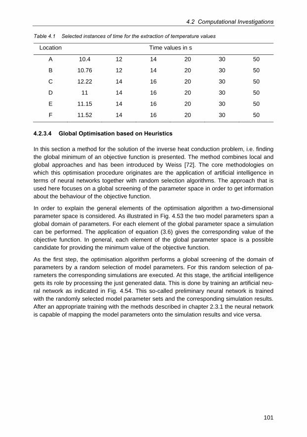
4.2 Computational Investigations
101
Table 4.1 Selected instances of time for the extraction of temperature values
Location Time values in s
A 10.4 12 14 20 30 50
B 10.76 12 14 20 30 50
C 12.22 14 16 20 30 50
D 11 14 16 20 30 50
E 11.15 14 16 20 30 50
F 11.52 14 16 20 30 50
4.2.3.4 Global Optimisation based on Heuristics
In this section a method for the solution of the inverse heat conduction problem, i.e. finding the global minimum of an objective function is presented. The method combines local and global approaches and has been introduced by Weiss [72]. The core methodologies on which this optimisation procedure originates are the application of artificial intelligence in terms of neural networks together with random selection algorithms. The approach that is used here focuses on a global screening of the parameter space in order to get information about the behaviour of the objective function.
In order to explain the general elements of the optimisation algorithm a two-dimensional parameter space is considered. As illustrated in Fig. 4.53 the two model parameters span a global domain of parameters. For each element of the global parameter space a simulation can be performed. The application of equation (3.6) gives the corresponding value of the objective function. In general, each element of the global parameter space is a possible candidate for providing the minimum value of the objective function.
As the first step, the optimisation algorithm performs a global screening of the domain of parameters by a random selection of model parameters. For this random selection of pa-rameters the corresponding simulations are executed. At this stage, the artificial intelligence gets its role by processing the just generated data. This is done by training an artificial neu-ral network as indicated in Fig. 4.54. This so-called preliminary neural network is trained with the randomly selected model parameter sets and the corresponding simulation results. After an appropriate training with the methods described in chapter 2.3.1 the neural network is capable of mapping the model parameters onto the simulation results and vice versa.
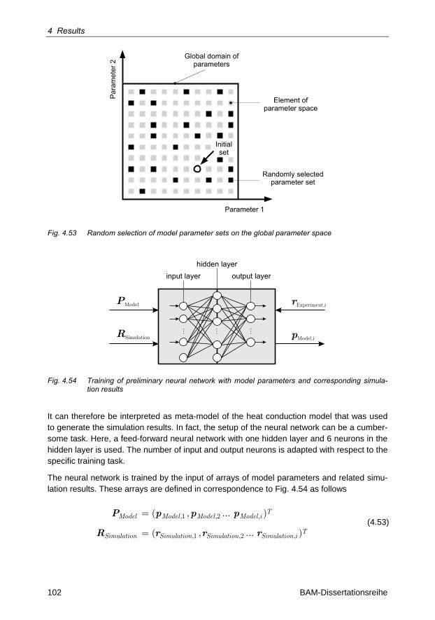
4 Results
102 BAM-Dissertationsreihe
Parameter 1
Initialset
Par
amet
er 2
Element ofparameter space
Randomly selectedparameter set
Global domain ofparameters
Fig. 4.53 Random selection of model parameter sets on the global parameter space
...... ...
PModel
RSimulation
rExperiment,i
pModel,i
input layerhidden layer
output layer
...
Fig. 4.54 Training of preliminary neural network with model parameters and corresponding simula-tion results
It can therefore be interpreted as meta-model of the heat conduction model that was used to generate the simulation results. In fact, the setup of the neural network can be a cumber-some task. Here, a feed-forward neural network with one hidden layer and 6 neurons in the hidden layer is used. The number of input and output neurons is adapted with respect to the specific training task.
The neural network is trained by the input of arrays of model parameters and related simu-lation results. These arrays are defined in correspondence to Fig. 4.54 as follows
TModel Model Model Model i
TSimulation Simulation Simulation Simulation i
,1 ,2 ,
,1 ,2 ,
( , ... )
( , ... )
=
=
P p p p
R r r r (4.53)
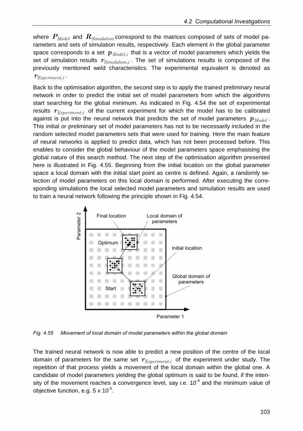
4.2 Computational Investigations
103
where ModelP and SimulationR correspond to the matrices composed of sets of model pa-rameters and sets of simulation results, respectively. Each element in the global parameter space corresponds to a set Model i,p that is a vector of model parameters which yields the set of simulation results Simulation i,r . The set of simulations results is composed of the previously mentioned weld characteristics. The experimental equivalent is denoted as
Experiment i,r .
Back to the optimisation algorithm, the second step is to apply the trained preliminary neural network in order to predict the initial set of model parameters from which the algorithms start searching for the global minimum. As indicated in Fig. 4.54 the set of experimental results Experiment i,r of the current experiment for which the model has to be calibrated against is put into the neural network that predicts the set of model parameters Modelp . This initial or preliminary set of model parameters has not to be necessarily included in the random selected model parameters sets that were used for training. Here the main feature of neural networks is applied to predict data, which has not been processed before. This enables to consider the global behaviour of the model parameters space emphasising the global nature of this search method. The next step of the optimisation algorithm presented here is illustrated in Fig. 4.55. Beginning from the initial location on the global parameter space a local domain with the initial start point as centre is defined. Again, a randomly se-lection of model parameters on this local domain is performed. After executing the corre-sponding simulations the local selected model parameters and simulation results are used to train a neural network following the principle shown in Fig. 4.54.
Parameter 1
Par
amet
er 2 Local domain of
parameters
Global domain ofparameters
Start
OptimumInitial location
Final location
Fig. 4.55 Movement of local domain of model parameters within the global domain
The trained neural network is now able to predict a new position of the centre of the local domain of parameters for the same set Experiment i,r of the experiment under study. The repetition of that process yields a movement of the local domain within the global one. A candidate of model parameters yielding the global optimum is said to be found, if the inten-sity of the movement reaches a convergence level, say i.e. 10-4 and the minimum value of objective function, e.g. 5 x 10⁻⁵.
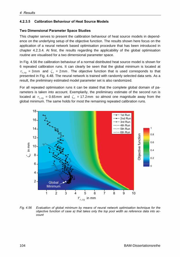
4 Results
104 BAM-Dissertationsreihe
4.2.3.5 Calibration Behaviour of Heat Source Models
Two Dimensional Parameter Space Studies This chapter serves to present the calibration behaviour of heat source models in depend-ence on the underlying setup of the objective function. The results shown here focus on the application of a neural network based optimisation procedure that has been introduced in chapter 4.2.3.4. At first, the results regarding the applicability of the global optimisation routine are visualised for a two dimensional parameter space.
In Fig. 4.56 the calibration behaviour of a normal distributed heat source model is shown for 6 repeated calibration runs. It can clearly be seen that the global minimum is located at
e xyr , = 3mm and ez = 2mm . The objective function that is used corresponds to that presented in Fig. 4.48. The neural network is trained with randomly selected data sets. As a result, the preliminary estimated model parameter set is also randomized.
For all repeated optimisation runs it can be stated that the complete global domain of pa-rameters is taken into account. Exemplarily, the preliminary estimate of the second run is located at e xyr , = 0.65mm and ez = 17.2mm so almost one magnitude away from the global minimum. The same holds for most the remaining repeated calibration runs.
1 2 3 4 5 6 7 8 9 10
2
4
6
8
10
12
14
16
181st Run2nd Run3rd Run4th Run5th Run6th Run
0
0.2
0.4
0.6
0.8
1
Obj
ectiv
e fu
nctio
n
GlobalMinimum
re,xy in mm
� ein
mm
Fig. 4.56 Evaluation of global minimum by means of neural network optimisation technique for the objective function of case a) that takes only the top pool width as reference data into ac-count
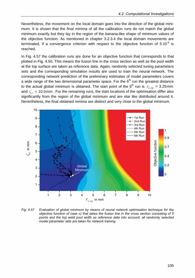
4.2 Computational Investigations
105
Nevertheless, the movement on the local domain goes into the direction of the global mini-mum. It is shown that the final minima of all the calibration runs do not match the global minimum exactly but they lay in the region of the banana-like shape of minimum values of the objective function. As mentioned in chapter 3.2.3.4 the local domain movements are terminated, if a convergence criterion with respect to the objective function of 5·10-5 is reached.
In Fig. 4.57 the calibration runs are done for an objective function that corresponds to that plotted in Fig. 4.50. This means the fusion line in the cross section as well as the pool width at the top surface are taken as reference data. Again, randomly selected tuning parameters sets and the corresponding simulation results are used to train the neural network. The corresponding network prediction of the preliminary estimates of model parameters covers a wide range of the two dimensional parameter space. For the 6th run the greatest distance to the actual global minimum is obtained. The start point of the 6th run is e xyr , = 3.25mm and ez = 10.0mm . For the remaining runs, the start locations of the optimisation differ also significantly from the region of the global minimum and are star like distributed around it. Nevertheless, the final obtained minima are distinct and very close to the global minimum.
1 2 3 4 5 6 7 8 9 10
1
2
3
4
5
6
7
8
9
10
1st Run2nd Run3rd Run4th Run5th Run6th Run
0
0.2
0.4
0.7
0.9
1
Obj
ectiv
e fu
nctio
n
GlobalMinimum
re,xy in mm
� ein
mm
Fig. 4.57 Evaluation of global minimum by means of neural network optimisation technique for the objective function of case c) that takes the fusion line in the cross section consisting of 5 points and the top weld pool width as reference data into account; all randomly selected model parameter sets are taken for network training
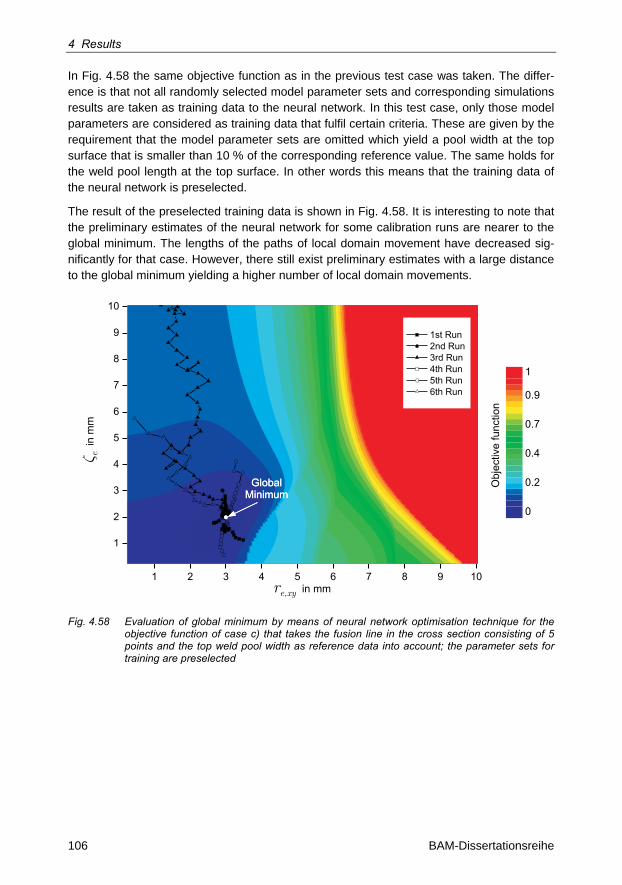
4 Results
106 BAM-Dissertationsreihe
In Fig. 4.58 the same objective function as in the previous test case was taken. The differ-ence is that not all randomly selected model parameter sets and corresponding simulations results are taken as training data to the neural network. In this test case, only those model parameters are considered as training data that fulfil certain criteria. These are given by the requirement that the model parameter sets are omitted which yield a pool width at the top surface that is smaller than 10 % of the corresponding reference value. The same holds for the weld pool length at the top surface. In other words this means that the training data of the neural network is preselected.
The result of the preselected training data is shown in Fig. 4.58. It is interesting to note that the preliminary estimates of the neural network for some calibration runs are nearer to the global minimum. The lengths of the paths of local domain movement have decreased sig-nificantly for that case. However, there still exist preliminary estimates with a large distance to the global minimum yielding a higher number of local domain movements.
1 2 3 4 5 6 7 8 9 10
1
2
3
4
5
6
7
8
9
10
1st Run2nd Run3rd Run4th Run5th Run6th Run
0
0.2
0.4
0.7
0.9
1
Obj
ectiv
e fu
nctio
nGlobal
MinimumGlobal
Minimum
re,xy in mm
� ein
mm
Fig. 4.58 Evaluation of global minimum by means of neural network optimisation technique for the objective function of case c) that takes the fusion line in the cross section consisting of 5 points and the top weld pool width as reference data into account; the parameter sets for training are preselected
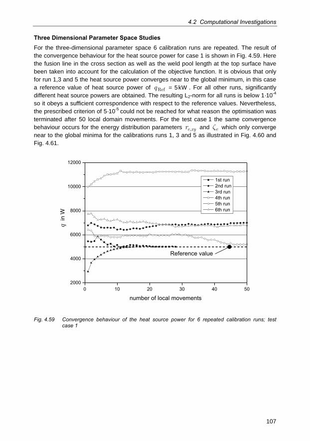
4.2 Computational Investigations
107
Three Dimensional Parameter Space Studies For the three-dimensional parameter space 6 calibration runs are repeated. The result of the convergence behaviour for the heat source power for case 1 is shown in Fig. 4.59. Here the fusion line in the cross section as well as the weld pool length at the top surface have been taken into account for the calculation of the objective function. It is obvious that only for run 1,3 and 5 the heat source power converges near to the global minimum, in this case a reference value of heat source power of qRef = 5kW . For all other runs, significantly different heat source powers are obtained. The resulting L2-norm for all runs is below 1·10-4 so it obeys a sufficient correspondence with respect to the reference values. Nevertheless, the prescribed criterion of 5·10-5 could not be reached for what reason the optimisation was terminated after 50 local domain movements. For the test case 1 the same convergence behaviour occurs for the energy distribution parameters e xyr , and ez which only converge near to the global minima for the calibrations runs 1, 3 and 5 as illustrated in Fig. 4.60 and Fig. 4.61.
0 10 20 30 40 502000
4000
6000
8000
10000
12000
number of local movements
1st run2nd run3rd run4th run5th run6th run
Reference value
qin
W
Fig. 4.59 Convergence behaviour of the heat source power for 6 repeated calibration runs; test case 1
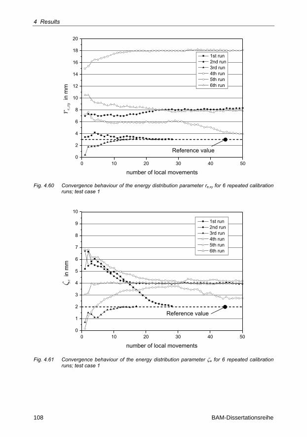
4 Results
108 BAM-Dissertationsreihe
0 10 20 30 40 500
2
4
6
8
10
12
14
16
18
20
number of local movements
1st run2nd run3rd run4th run5th run6th run
Reference value
r e,x
yin
mm
Fig. 4.60 Convergence behaviour of the energy distribution parameter re,xy for 6 repeated calibration runs; test case 1
0 10 20 30 40 500
1
2
3
4
5
6
7
8
9
10
number of local movements
1st run2nd run3rd run4th run5th run6th run
Reference value
� ein
mm
Fig. 4.61 Convergence behaviour of the energy distribution parameter e for 6 repeated calibration runs; test case 1
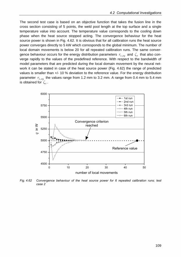
4.2 Computational Investigations
109
The second test case is based on an objective function that takes the fusion line in the cross section consisting of 5 points, the weld pool length at the top surface and a single temperature value into account. The temperature value corresponds to the cooling down phase when the heat source stopped acting. The convergence behaviour for the heat source power is shown in Fig. 4.62. It is obvious that for all calibration runs the heat source power converges directly to 5 kW which corresponds to the global minimum. The number of local domain movements is below 20 for all repeated calibration runs. The same conver-gence behaviour occurs for the energy distribution parameters e xyr , and ez that also con-verge rapidly to the values of the predefined reference. With respect to the bandwidth of model parameters that are predicted during the local domain movement by the neural net-work it can be stated in case of the heat source power (Fig. 4.62) the range of predicted values is smaller than +/- 10 % deviation to the reference value. For the energy distribution parameter e xyr , the values range from 1.2 mm to 3.2 mm. A range from 0.4 mm to 5.4 mm is obtained for ez .
0 10 20 30 40 504500
4750
5000
5250
5500
5750
6000
number of local movements
1st run2nd run3rd run4th run5th run6th run
Reference value
qin
W
Convergence criterionreached
Fig. 4.62 Convergence behaviour of the heat source power for 6 repeated calibration runs; test case 2
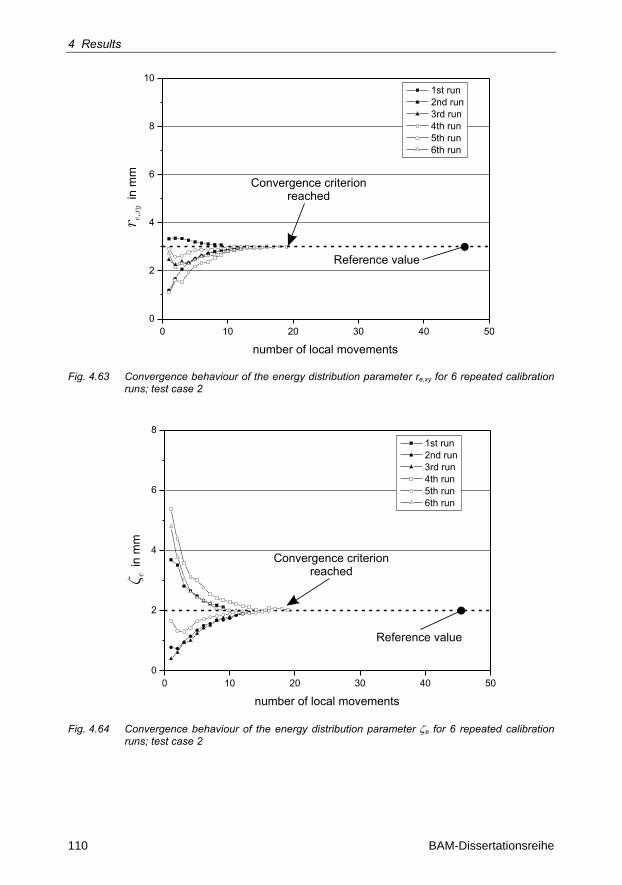
4 Results
110 BAM-Dissertationsreihe
0 10 20 30 40 500
2
4
6
8
10
number of local movements
1st run2nd run3rd run4th run5th run6th run
Reference value
r e,x
yin
mm
Convergence criterionreached
Fig. 4.63 Convergence behaviour of the energy distribution parameter re,xy for 6 repeated calibration runs; test case 2
� ein
mm
0 10 20 30 40 500
2
4
6
8
number of local movements
1st run2nd run3rd run4th run5th run6th run
Reference value
Convergence criterionreached
Fig. 4.64 Convergence behaviour of the energy distribution parameter e for 6 repeated calibration runs; test case 2
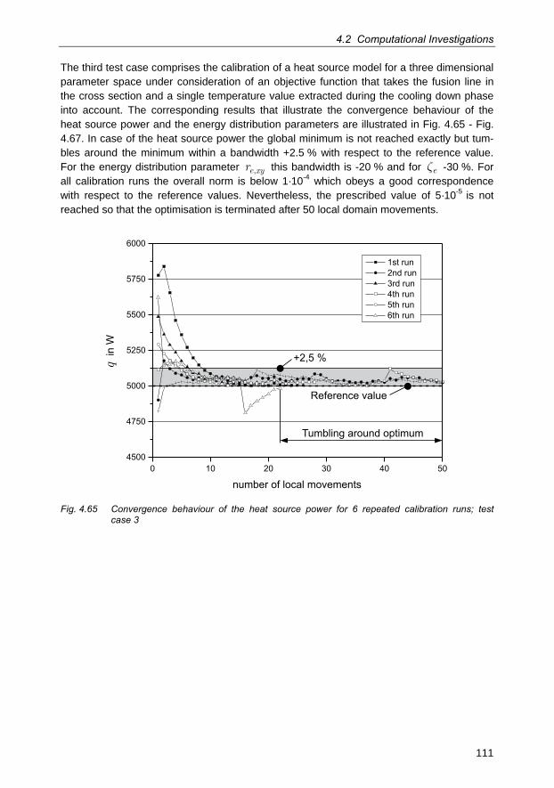
4.2 Computational Investigations
111
The third test case comprises the calibration of a heat source model for a three dimensional parameter space under consideration of an objective function that takes the fusion line in the cross section and a single temperature value extracted during the cooling down phase into account. The corresponding results that illustrate the convergence behaviour of the heat source power and the energy distribution parameters are illustrated in Fig. 4.65 - Fig. 4.67. In case of the heat source power the global minimum is not reached exactly but tum-bles around the minimum within a bandwidth +2.5 % with respect to the reference value. For the energy distribution parameter e xyr , this bandwidth is -20 % and for ez -30 %. For all calibration runs the overall norm is below 1·10-4 which obeys a good correspondence with respect to the reference values. Nevertheless, the prescribed value of 5·10-5 is not reached so that the optimisation is terminated after 50 local domain movements.
0 10 20 30 40 504500
4750
5000
5250
5500
5750
6000
number of local movements
1st run2nd run3rd run4th run5th run6th run
Reference value
+2,5 %
Tumbling around optimum
qin
W
Fig. 4.65 Convergence behaviour of the heat source power for 6 repeated calibration runs; test case 3
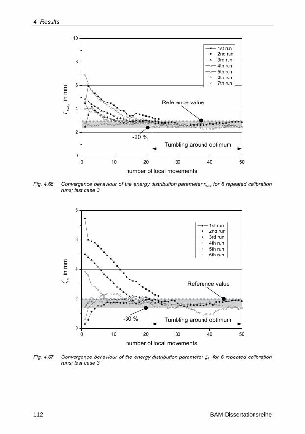
4 Results
112 BAM-Dissertationsreihe
0 10 20 30 40 500
2
4
6
8
10
number of local movements
1st run2nd run3rd run4th run5th run6th run7th run
Reference value
-20 %Tumbling around optimum
r e,x
yin
mm
Fig. 4.66 Convergence behaviour of the energy distribution parameter re,xy for 6 repeated calibration runs; test case 3
0 10 20 30 40 500
2
4
6
8
number of local movements
1st run2nd run3rd run4th run5th run6th run
Reference value
-30 % Tumbling around optimum
� ein
mm
Fig. 4.67 Convergence behaviour of the energy distribution parameter e for 6 repeated calibration runs; test case 3
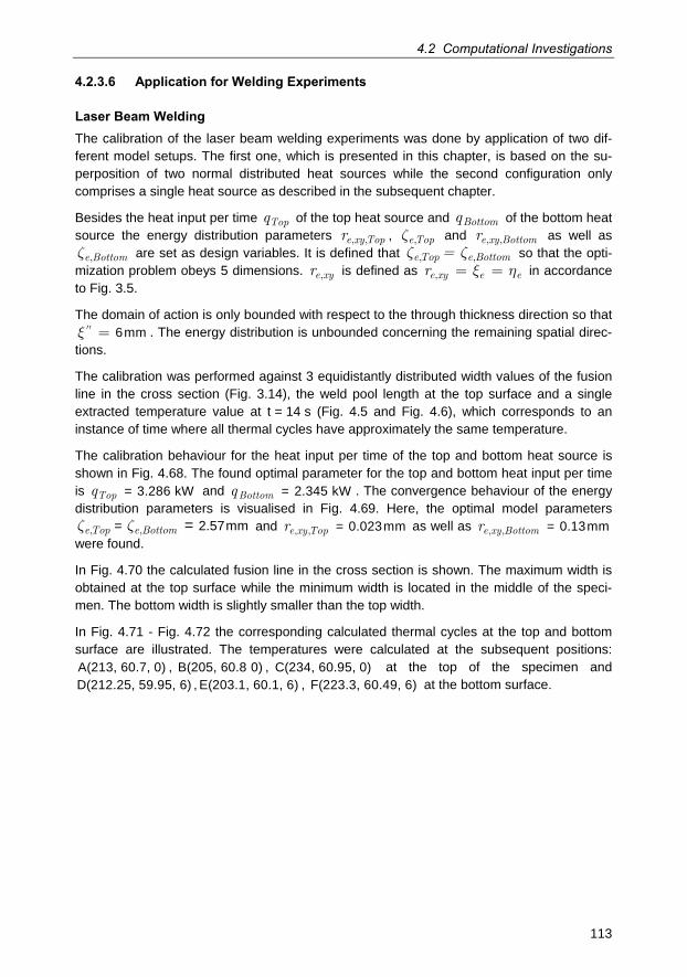
4.2 Computational Investigations
113
4.2.3.6 Application for Welding Experiments
Laser Beam Welding The calibration of the laser beam welding experiments was done by application of two dif-ferent model setups. The first one, which is presented in this chapter, is based on the su-perposition of two normal distributed heat sources while the second configuration only comprises a single heat source as described in the subsequent chapter.
Besides the heat input per time Topq of the top heat source and Bottomq of the bottom heat source the energy distribution parameters e xy Topr , , , e Top,z and e xy Bottomr , , as well as
e Bottom,z are set as design variables. It is defined that eTop e Bottom=, ,z z so that the opti-mization problem obeys 5 dimensions. e xyr , is defined as e xy e er , x h= = in accordance to Fig. 3.5.
The domain of action is only bounded with respect to the through thickness direction so that ''x = 6mm . The energy distribution is unbounded concerning the remaining spatial direc-
tions.
The calibration was performed against 3 equidistantly distributed width values of the fusion line in the cross section (Fig. 3.14), the weld pool length at the top surface and a single extracted temperature value at t = 14 s (Fig. 4.5 and Fig. 4.6), which corresponds to an instance of time where all thermal cycles have approximately the same temperature.
The calibration behaviour for the heat input per time of the top and bottom heat source is shown in Fig. 4.68. The found optimal parameter for the top and bottom heat input per time is Topq = 3.286 kW and Bottomq = 2.345 kW . The convergence behaviour of the energy distribution parameters is visualised in Fig. 4.69. Here, the optimal model parameters
eTop e Bottom, ,z z= 2.57mm= and e xy Topr , , = 0.023mm as well as e xy Bottomr , , = 0.13mm were found.
In Fig. 4.70 the calculated fusion line in the cross section is shown. The maximum width is obtained at the top surface while the minimum width is located in the middle of the speci-men. The bottom width is slightly smaller than the top width.
In Fig. 4.71 - Fig. 4.72 the corresponding calculated thermal cycles at the top and bottom surface are illustrated. The temperatures were calculated at the subsequent positions: A(213, 60.7, 0) , B(205, 60.8 0) , 60.C(234, 95, 0) at the top of the specimen and D(212.25, 59.95, 6) , E(203.1, 60.1, 6) , F(223.3, 60.49, 6) at the bottom surface.
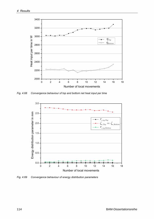
4 Results
114 BAM-Dissertationsreihe
qTop
qBottom
0 2 4 6 8 10 12 14 16 182000
2200
2400
2600
2800
3000
3200
3400
Hea
tinp
utpe
rtim
ein
W
Number of local movements
Fig. 4.68 Convergence behaviour of top and bottom net heat input per time
0 2 4 6 8 10 12 14 16 180.0
0.5
1.0
1.5
2.0
2.5
3.0
Ene
rgy
dist
ribut
ion
para
met
erin
mm
Number of local movements
� �e,Top e,Bottom=re,xy,Top
re,xy,Bottom
Fig. 4.69 Convergence behaviour of energy distribution parameters
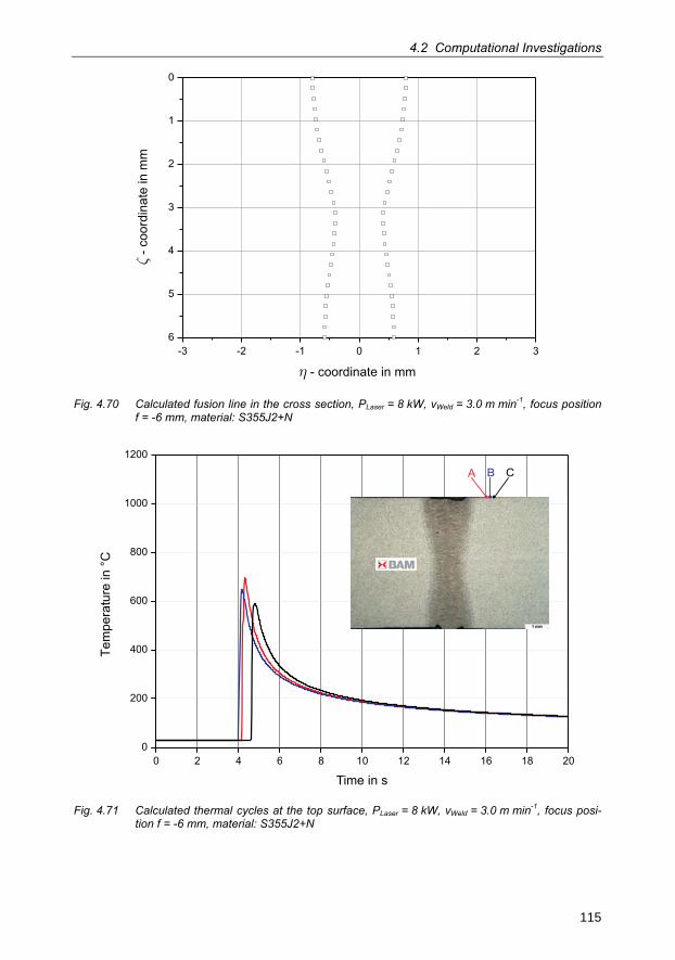
4.2 Computational Investigations
115
-3 -2 -1 0 1 2 36
5
4
3
2
1
0
� - coordinate in mm
�- c
oord
inat
e in
mm
Fig. 4.70 Calculated fusion line in the cross section, PLaser = 8 kW, vWeld = 3.0 m min-1, focus position f = -6 mm, material: S355J2+N
0 2 4 6 8 10 12 14 16 18 200
200
400
600
800
1000
1200
Tem
pera
ture
in°C
Time in s
CBA
Fig. 4.71 Calculated thermal cycles at the top surface, PLaser = 8 kW, vWeld = 3.0 m min-1, focus posi-tion f = -6 mm, material: S355J2+N
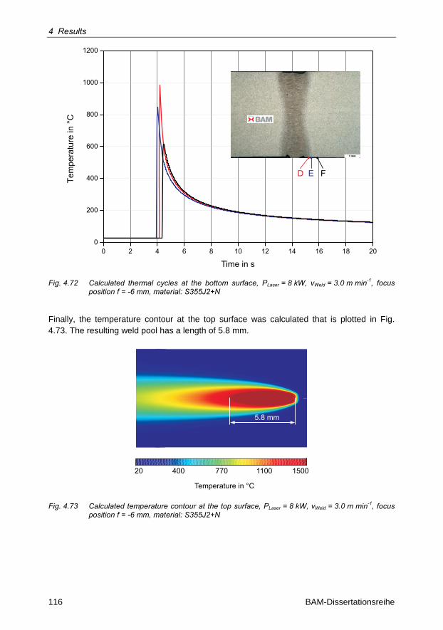
4 Results
116 BAM-Dissertationsreihe
0 2 4 6 8 10 12 14 16 18 200
200
400
600
800
1000
1200
Tem
pera
ture
in°C
Time in s
ED F
Fig. 4.72 Calculated thermal cycles at the bottom surface, PLaser = 8 kW, vWeld = 3.0 m min-1, focus position f = -6 mm, material: S355J2+N
Finally, the temperature contour at the top surface was calculated that is plotted in Fig. 4.73. The resulting weld pool has a length of 5.8 mm.
2 mm
20 400 770 1100 1500
Temperature in °C
5.8 mm
Fig. 4.73 Calculated temperature contour at the top surface, PLaser = 8 kW, vWeld = 3.0 m min-1, focus position f = -6 mm, material: S355J2+N
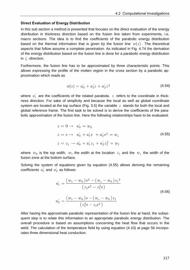
4.2 Computational Investigations
117
Direct Evaluation of Energy Distribution In this sub section a method is presented that focuses on the direct evaluation of the energy distribution in thickness direction based on the fusion line taken from experiments, i.e. macro sections. The idea is to find the coefficients of the parabolic energy distribution based on the thermal information that is given by the fusion line w z( ) . The theoretical aspects that follow assume a complete penetration. As indicated in Fig. 4.74 the derivation of the energy distribution based on the fusion line is done for a parabolic energy distribution in z -direction.
Furthermore, the fusion line has to be approximated by three characteristic points. This allows expressing the profile of the molten region in the cross section by a parabolic ap-proximation which reads as
' ' 'w z a a z a z 20 1 2( ) = + + (4.54)
where 'ia are the coefficients of the related parabola. z refers to the coordinate in thick-
ness direction. For sake of simplicity and because the local as well as global coordinate system are located at the top surface (Fig. 3.5) the variable z stands for both the local and global reference frame. The first task to be solved is to derive the coefficients of the para-bolic approximation of the fusion line. Here the following relationships have to be evaluated:
'
' ' 's
' ' '
z a w
z s a a s a s w
z z a a z a z w
0 0
20 1 2
21 0 1 1 2 11
0 ==
= + + =
= + + =
(4.55)
where w0 is the top width, w1 the width at the location z1 and the sw the width of the fusion zone at the bottom surface.
Solving the system of equations given by equation (4.55) allows deriving the remaining coefficients 'a1 and 'a2 as follows:
( ) ( )( )
( ) ( )( )
s'
s'
w w s w w za
z s z s
w w s w w za
z s z s
2 21 0 0 1
1 221 1
1 0 0 12 2 2
11
- - -=
-
- - -=
-
(4.56)
After having the approximate parabolic representation of the fusion line at hand, the subse-quent step is to relate this information to an appropriate parabolic energy distribution. The overall procedure is based on assumptions concerning the heat flow that occurs in the weld. The calculation of the temperature field by using equation (4.10) at page 56 incorpo-rates three dimensional heat conduction.
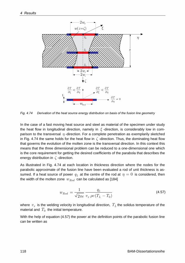
4 Results
118 BAM-Dissertationsreihe
s
�
�
w z( = )� �
wRod
1T
0�
��
�
T T
� �
� �
� ��
T T
� �
� �
� ��
2ws
2w1
2w0
z0
z1
zs
Fig. 4.74 Derivation of the heat source energy distribution on basis of the fusion line geometry
In the case of a fast moving heat source and steel as material of the specimen under study the heat flow in longitudinal direction, namely in x -direction, is considerably low in com-parison to the transversal h -direction. For a complete penetration as exemplarily sketched in Fig. 4.74 the same holds for the heat flow in z -direction. Thus, the dominating heat flow that governs the evolution of the molten zone is the transversal direction. In this context this means that the three dimensional problem can be reduced to a one-dimensional one which is the core requirement for getting the desired coefficients of the parabola that describes the energy distribution in z -direction.
As illustrated in Fig. 4.74 at each location in thickness direction where the nodes for the parabolic approximate of the fusion line have been evaluated a rod of unit thickness is as-sumed. If a heat source of power q1 at the centre of the rod at 0h = is considered, then the width of the molten zone Rodw can be calculated as [184]
Rodx L
qw
v c T Te
1
0
1
( )2 rp=
- (4.57)
where xv is the welding velocity in longitudinal direction, LT the solidus temperature of the material and T0 the initial temperature.
With the help of equation (4.57) the power at the definition points of the parabolic fusion line can be written as
4.2 Computational Investigations
119
x L
const A
q z w z e v c T T w z A1 0( ) ( ) 2 ( ) ( )p r
= =
= - =
(4.58)
where w z( ) corresponds to the widths w0 , w1 and sw and q z1( ) to the needed power to achieve these fusion widths.
The power is also set to have a parabolic distribution. Incorporating equation (4.54) this allows deriving the following relationship:
( )
' ' '
' ' '
a a a
q z w z A A a a z a z
Aa Aa z Aa z
0 1 2
21 0 1 2
20 1 2
( ) ( ) =
* * *
= + +
= + + (4.59)
which is the desired parabolic energy distribution that yields the width of the fusion line at the locations z 0 , z1 and sz .
The coefficients ia * determine the shape of the energy distribution along the local z -axis. In contrast to equation (3.4) the dimension of the coefficients are different. The fact requires taking the heat input of the heat source into account correctly. That can be achieved by an normalisation with respect to the net power. In other words it means that equation (4.59) refers to the product f q( )z . Therefore, the coefficients of equation (4.59) have to be recal-culated in order to provide the unit parabolic power distribution as requested by the func-tional-analytical simulation framework ( equation (3.4) ).
In the laser beam welding example that has been introduced in chapter 3.1 the cross sec-tion can be described by the following points (Fig. 3.14): TopP (1.6,0) , MiddleP (0.9,3) and BottomP (1.2,6) . At first, the constant A is evaluated which yields for the given material and welding conditions
A 9 -31.756 10 kgs= ´ (4.60)
In reference to the geometry of the fusion line the coefficients a *0 , a *
1 and a *2 equate as
follows:
a
a
a
* 6 -10
* 8 -21
* 10 -32
2.81×10 Wm
-7.02×10 Wm
9.76×10 Wm
=
=
=
(4.61)
This allows deriving the energy distribution in z -direction on basis of equation (4.59).
These coefficients need to be normalised with respect to the net heat input per time (power). Thus, a concentrated line source is calibrated against a single temperature value extracted at t = 14 s out of the experimental thermal cycle. The corresponding convergence
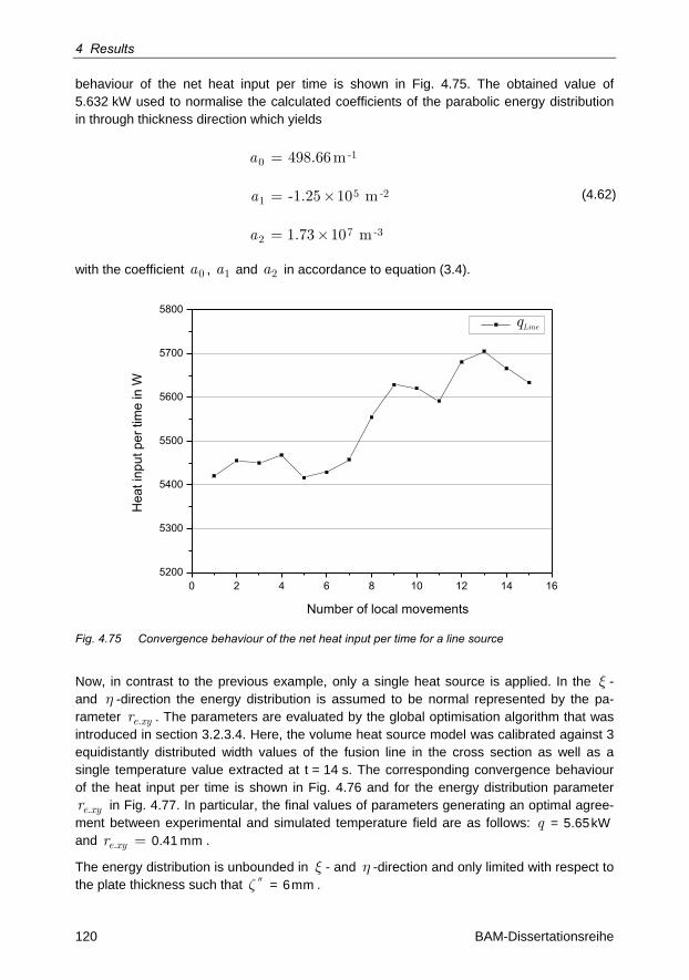
4 Results
120 BAM-Dissertationsreihe
behaviour of the net heat input per time is shown in Fig. 4.75. The obtained value of 5.632 kW used to normalise the calculated coefficients of the parabolic energy distribution in through thickness direction which yields
a
a
a
-10
5 -21
7 -32
498.66m
-1.25×10 m
1.73×10 m
=
=
=
(4.62)
with the coefficient a0 , a1 and a2 in accordance to equation (3.4).
0 2 4 6 8 10 12 14 165200
5300
5400
5500
5600
5700
5800
Hea
tinp
utpe
rtim
ein
W
qLine
Number of local movements
Fig. 4.75 Convergence behaviour of the net heat input per time for a line source
Now, in contrast to the previous example, only a single heat source is applied. In the x - and h -direction the energy distribution is assumed to be normal represented by the pa-rameter e xyr . . The parameters are evaluated by the global optimisation algorithm that was introduced in section 3.2.3.4. Here, the volume heat source model was calibrated against 3 equidistantly distributed width values of the fusion line in the cross section as well as a single temperature value extracted at t = 14 s. The corresponding convergence behaviour of the heat input per time is shown in Fig. 4.76 and for the energy distribution parameter
e xyr . in Fig. 4.77. In particular, the final values of parameters generating an optimal agree-ment between experimental and simulated temperature field are as follows: q = 5.65kW and e xyr . = 0.41 mm .
The energy distribution is unbounded in x - and h -direction and only limited with respect to the plate thickness such that z = 6mm .
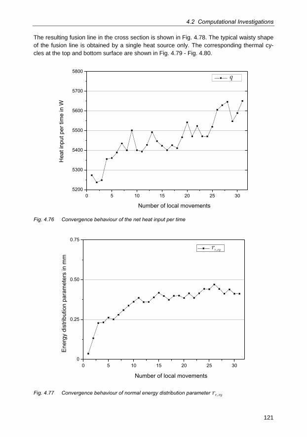
4.2 Computational Investigations
121
The resulting fusion line in the cross section is shown in Fig. 4.78. The typical waisty shape of the fusion line is obtained by a single heat source only. The corresponding thermal cy-cles at the top and bottom surface are shown in Fig. 4.79 - Fig. 4.80.
0 5 10 15 20 25 305200
5300
5400
5500
5600
5700
5800
Hea
tinp
utpe
rtim
ein
W
q
Number of local movements
Fig. 4.76 Convergence behaviour of the net heat input per time
0 5 10 15 20 25 300
0.25
0.50
0.75
Ene
rgy
dist
ribut
ion
para
met
ers
inm
m
re,xy
Number of local movements
Fig. 4.77 Convergence behaviour of normal energy distribution parameter re,xy
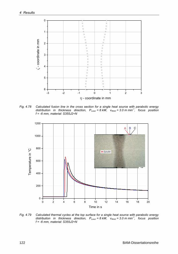
4 Results
122 BAM-Dissertationsreihe
� - coordinate in mm
�- c
oord
inat
e in
mm
-3 -2 -1 0 1 2 36
5
4
3
2
1
0
Fig. 4.78 Calculated fusion line in the cross section for a single heat source with parabolic energy distribution in thickness direction, PLaser = 8 kW, vWeld = 3.0 m min-1, focus position f = -6 mm, material: S355J2+N
0 2 4 6 8 10 12 14 16 18 200
200
400
600
800
1000
1200
Tem
pera
ture
in°C
Time in s
CBA
Fig. 4.79 Calculated thermal cycles at the top surface for a single heat source with parabolic energy distribution in thickness direction, PLaser = 8 kW, vWeld = 3.0 m min-1, focus position f = -6 mm, material: S355J2+N
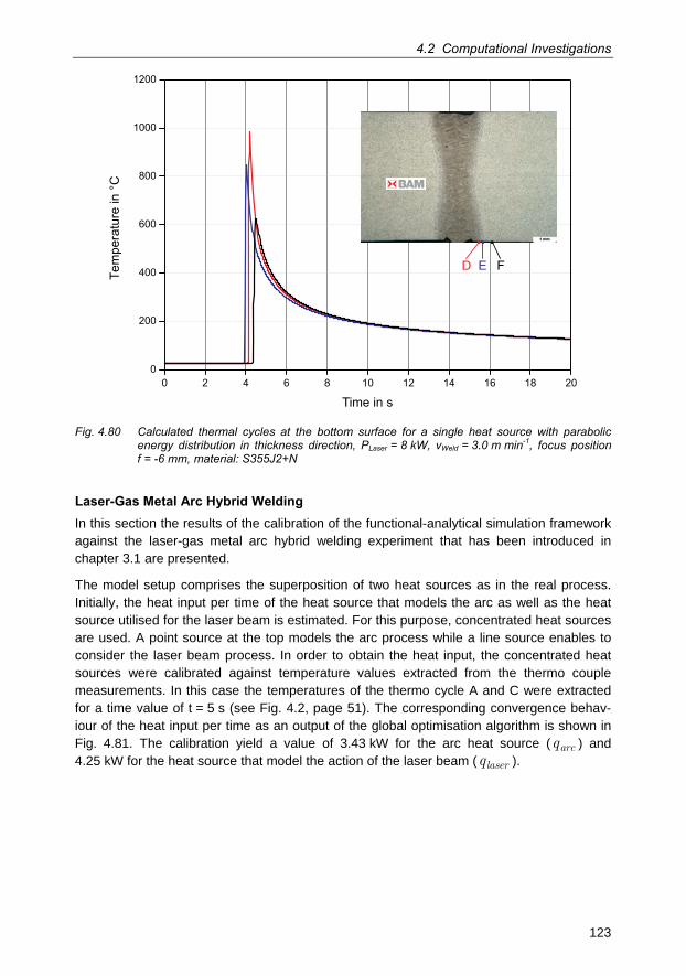
4.2 Computational Investigations
123
0 2 4 6 8 10 12 14 16 18 200
200
400
600
800
1000
1200
Tem
pera
ture
in°C
Time in s
ED F
Fig. 4.80 Calculated thermal cycles at the bottom surface for a single heat source with parabolic energy distribution in thickness direction, PLaser = 8 kW, vWeld = 3.0 m min-1, focus position f = -6 mm, material: S355J2+N
Laser-Gas Metal Arc Hybrid Welding In this section the results of the calibration of the functional-analytical simulation framework against the laser-gas metal arc hybrid welding experiment that has been introduced in chapter 3.1 are presented.
The model setup comprises the superposition of two heat sources as in the real process. Initially, the heat input per time of the heat source that models the arc as well as the heat source utilised for the laser beam is estimated. For this purpose, concentrated heat sources are used. A point source at the top models the arc process while a line source enables to consider the laser beam process. In order to obtain the heat input, the concentrated heat sources were calibrated against temperature values extracted from the thermo couple measurements. In this case the temperatures of the thermo cycle A and C were extracted for a time value of t = 5 s (see Fig. 4.2, page 51). The corresponding convergence behav-iour of the heat input per time as an output of the global optimisation algorithm is shown in Fig. 4.81. The calibration yield a value of 3.43 kW for the arc heat source ( arcq ) and 4.25 kW for the heat source that model the action of the laser beam ( laserq ).
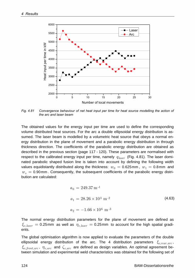
4 Results
124 BAM-Dissertationsreihe
0 5 10 15 20 25 302000
2500
3000
3500
4000
4500
5000
5500
6000
Hea
tinp
utpe
rtim
ein
kW
Number of local movements
LaserArc
Fig. 4.81 Convergence behaviour of net heat input per time for heat source modelling the action of the arc and laser beam
The obtained values for the energy input per time are used to define the corresponding volume distributed heat sources. For the arc a double ellipsoidal energy distribution is as-sumed. The laser beam is modelled by a volumetric heat source that obeys a normal en-ergy distribution in the plane of movement and a parabolic energy distribution in through thickness direction. The coefficients of the parabolic energy distribution are obtained as described in the previous section (page 117 - 120). These parameters are normalised with respect to the calibrated energy input per time, namely laserq (Fig. 4.81). The laser domi-nated parabolic shaped fusion line is taken into account by defining the following width values equidistantly distributed along the thickness: w 0 = 0.625mm , w1 = 0.8mm and
sw = 0.90mm . Consequently, the subsequent coefficients of the parabolic energy distri-bution are calculated:
a
a
a
-10
3 -21
6 -32
249.37 m
28.26×10 m
1.66×10 m
=
=
= -
(4.63)
The normal energy distribution parameters for the plane of movement are defined as
e laser,x = 0.25mm as well as e laser,h = 0.25mm to account for the high spatial gradi-ents.
The global optimisation algorithm is now applied to evaluate the parameters of the double ellipsoidal energy distribution of the arc. The 4 distribution parameters e rear arc, ,x ,
e front arc, ,x , e arc,h and e arc,z are defined as design variables. An optimal agreement be-tween simulation and experimental weld characteristics was obtained for the following set of
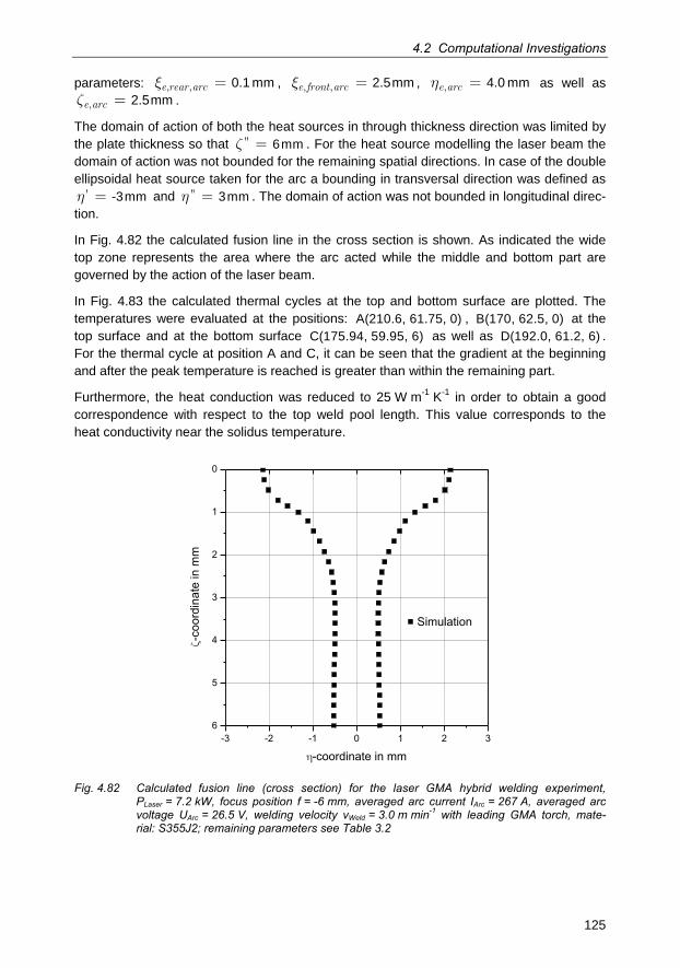
4.2 Computational Investigations
125
parameters: e rear arc, ,x = 0.1 mm , e front arc, ,x = 2.5mm , e arc,h = 4.0 mm as well as
e arc,z = 2.5mm .
The domain of action of both the heat sources in through thickness direction was limited by the plate thickness so that ''z = 6mm . For the heat source modelling the laser beam the domain of action was not bounded for the remaining spatial directions. In case of the double ellipsoidal heat source taken for the arc a bounding in transversal direction was defined as
'h = -3mm and ''h = 3mm . The domain of action was not bounded in longitudinal direc-tion.
In Fig. 4.82 the calculated fusion line in the cross section is shown. As indicated the wide top zone represents the area where the arc acted while the middle and bottom part are governed by the action of the laser beam.
In Fig. 4.83 the calculated thermal cycles at the top and bottom surface are plotted. The temperatures were evaluated at the positions: A(210.6, 61.75, 0) , B(170, 62.5, 0) at the top surface and at the bottom surface C(175.94, 59.95, 6) as well as D(192.0, 61.2, 6) . For the thermal cycle at position A and C, it can be seen that the gradient at the beginning and after the peak temperature is reached is greater than within the remaining part.
Furthermore, the heat conduction was reduced to 25 W m-1 K-1 in order to obtain a good correspondence with respect to the top weld pool length. This value corresponds to the heat conductivity near the solidus temperature.
-3 -2 -1 0 1 2 36
5
4
3
2
1
0
�-coordinate in mm
Simulation
-c
oord
inat
e in
mm
Fig. 4.82 Calculated fusion line (cross section) for the laser GMA hybrid welding experiment, PLaser = 7.2 kW, focus position f = -6 mm, averaged arc current IArc = 267 A, averaged arc voltage UArc = 26.5 V, welding velocity vWeld = 3.0 m min-1 with leading GMA torch, mate-rial: S355J2; remaining parameters see Table 3.2
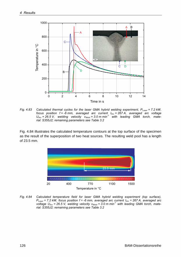
4 Results
126 BAM-Dissertationsreihe
0 2 4 6 8 10 12 140
200
400
600
800
1000
Time in s
D
BA
C
Tem
pera
ture
in °
CA
C
B D
Fig. 4.83 Calculated thermal cycles for the laser GMA hybrid welding experiment, PLaser = 7.2 kW, focus position f = -6 mm, averaged arc current IArc = 267 A, averaged arc voltage UArc = 26.5 V, welding velocity vWeld = 3.0 m min-1 with leading GMA torch, mate-rial: S355J2; remaining parameters see Table 3.2
Fig. 4.84 illustrates the calculated temperature contours at the top surface of the specimen as the result of the superposition of two heat sources. The resulting weld pool has a length of 23.5 mm.
20 400 770 1100 1500Temperature in °C
23.5 mm
Fig. 4.84 Calculated temperature field for laser GMA hybrid welding experiment (top surface), PLaser = 7.2 kW, focus position f = -6 mm, averaged arc current IArc = 267 A, averaged arc voltage UArc = 26.5 V, welding velocity vWeld = 3.0 m min-1 with leading GMA torch, mate-rial: S355J2; remaining parameters see Table 3.2
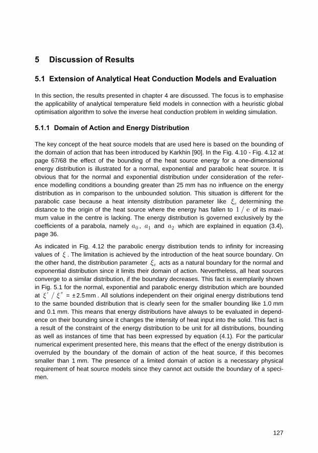
127
5 Discussion of Results
5.1 Extension of Analytical Heat Conduction Models and Evaluation
In this section, the results presented in chapter 4 are discussed. The focus is to emphasise the applicability of analytical temperature field models in connection with a heuristic global optimisation algorithm to solve the inverse heat conduction problem in welding simulation.
5.1.1 Domain of Action and Energy Distribution
The key concept of the heat source models that are used here is based on the bounding of the domain of action that has been introduced by Karkhin [90]. In the Fig. 4.10 - Fig. 4.12 at page 67/68 the effect of the bounding of the heat source energy for a one-dimensional energy distribution is illustrated for a normal, exponential and parabolic heat source. It is obvious that for the normal and exponential distribution under consideration of the refer-ence modelling conditions a bounding greater than 25 mm has no influence on the energy distribution as in comparison to the unbounded solution. This situation is different for the parabolic case because a heat intensity distribution parameter like ex determining the distance to the origin of the heat source where the energy has fallen to 1 / e of its maxi-mum value in the centre is lacking. The energy distribution is governed exclusively by the coefficients of a parabola, namely a0 , a1 and a2 which are explained in equation (3.4), page 36.
As indicated in Fig. 4.12 the parabolic energy distribution tends to infinity for increasing values of x . The limitation is achieved by the introduction of the heat source boundary. On the other hand, the distribution parameter ex acts as a natural boundary for the normal and exponential distribution since it limits their domain of action. Nevertheless, all heat sources converge to a similar distribution, if the boundary decreases. This fact is exemplarily shown in Fig. 5.1 for the normal, exponential and parabolic energy distribution which are bounded at /x x¢ = ± 2.5mm . All solutions independent on their original energy distributions tend to the same bounded distribution that is clearly seen for the smaller bounding like 1.0 mm and 0.1 mm. This means that energy distributions have always to be evaluated in depend-ence on their bounding since it changes the intensity of heat input into the solid. This fact is a result of the constraint of the energy distribution to be unit for all distributions, bounding as well as instances of time that has been expressed by equation (4.1). For the particular numerical experiment presented here, this means that the effect of the energy distribution is overruled by the boundary of the domain of action of the heat source, if this becomes smaller than 1 mm. The presence of a limited domain of action is a necessary physical requirement of heat source models since they cannot act outside the boundary of a speci-men.
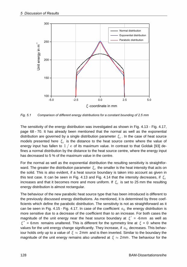
5 Discussion of Results
128 BAM-Dissertationsreihe
� -coordinate in mm
-5.0 -2.5 0.0 2.5 5.0100
150
200
250
300
Normal distribution
Exponential distribution
Parabolic distributionU
nite
nerg
yin
m-1
Fig. 5.1 Comparison of different energy distributions for a constant bounding of 2.5 mm
The sensitivity of the energy distribution was investigated as shown in Fig. 4.13 - Fig. 4.17, page 68 - 70. It has already been mentioned that the normal as well as the exponential distribution are governed by a single distribution parameter ex . In the case of heat source models presented here ex is the distance to the heat source centre where the value of energy input has fallen to 1 / e of its maximum value. In contrast to that Goldak [93] de-fines a normal distribution by the distance to the heat source centre, where the energy input has decreased to 5 % of the maximum value in the centre.
For the normal as well as the exponential distribution the resulting sensitivity is straightfor-ward. The greater the distribution parameter ex the smaller is the heat intensity that acts on the solid. This is also evident, if a heat source boundary is taken into account as given in this test case. It can be seen in Fig. 4.13 and Fig. 4.14 that the intensity decreases, if ex increases and that it becomes more and more uniform. If ex is set to 25 mm the resulting energy distribution is almost rectangular.
The behaviour of the new parabolic heat source type that has been introduced is different to the previously discussed energy distributions. As mentioned, it is determined by three coef-ficients which define the parabolic distribution. The sensitivity is not as straightforward as it can be seen in Fig. 4.15 - Fig. 4.17. In case of the coefficient a0 the energy distribution is more sensitive due to a decrease of the coefficient than to an increase. For both cases the magnitude of the unit energy near the heat source boundary at x ¢ = -6mm as well as x = 6mm remains unaltered. This is different for the symmetry line at x = 0 where the values for the unit energy change significantly. They increase, if a0 decreases. This behav-iour holds only up to a value of x » 2mm and is then inverted. Similar to the boundary the magnitude of the unit energy remains also unaltered at x » 2mm . The behaviour for the
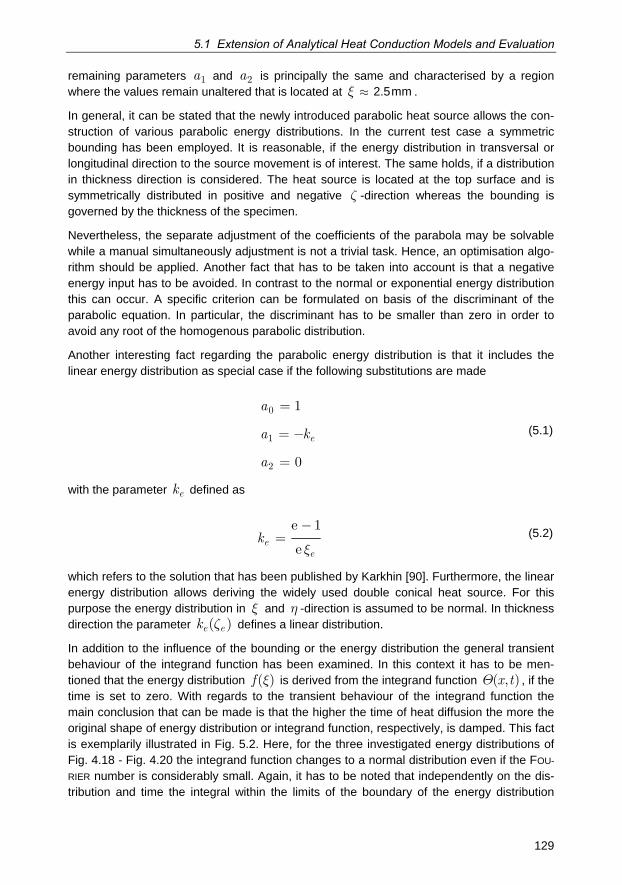
5.1 Extension of Analytical Heat Conduction Models and Evaluation
129
remaining parameters a1 and a2 is principally the same and characterised by a region where the values remain unaltered that is located at x » 2.5mm .
In general, it can be stated that the newly introduced parabolic heat source allows the con-struction of various parabolic energy distributions. In the current test case a symmetric bounding has been employed. It is reasonable, if the energy distribution in transversal or longitudinal direction to the source movement is of interest. The same holds, if a distribution in thickness direction is considered. The heat source is located at the top surface and is symmetrically distributed in positive and negative z -direction whereas the bounding is governed by the thickness of the specimen.
Nevertheless, the separate adjustment of the coefficients of the parabola may be solvable while a manual simultaneously adjustment is not a trivial task. Hence, an optimisation algo-rithm should be applied. Another fact that has to be taken into account is that a negative energy input has to be avoided. In contrast to the normal or exponential energy distribution this can occur. A specific criterion can be formulated on basis of the discriminant of the parabolic equation. In particular, the discriminant has to be smaller than zero in order to avoid any root of the homogenous parabolic distribution.
Another interesting fact regarding the parabolic energy distribution is that it includes the linear energy distribution as special case if the following substitutions are made
e
a
a k
a
0
1
2
1
0
=
= -
=
(5.1)
with the parameter ek defined as
ee
ke 1
e x
-= (5.2)
which refers to the solution that has been published by Karkhin [90]. Furthermore, the linear energy distribution allows deriving the widely used double conical heat source. For this purpose the energy distribution in x and h -direction is assumed to be normal. In thickness direction the parameter e ek ( )z defines a linear distribution.
In addition to the influence of the bounding or the energy distribution the general transient behaviour of the integrand function has been examined. In this context it has to be men-tioned that the energy distribution f ( )x is derived from the integrand function x t( , )Q , if the time is set to zero. With regards to the transient behaviour of the integrand function the main conclusion that can be made is that the higher the time of heat diffusion the more the original shape of energy distribution or integrand function, respectively, is damped. This fact is exemplarily illustrated in Fig. 5.2. Here, for the three investigated energy distributions of Fig. 4.18 - Fig. 4.20 the integrand function changes to a normal distribution even if the FOU-
RIER number is considerably small. Again, it has to be noted that independently on the dis-tribution and time the integral within the limits of the boundary of the energy distribution
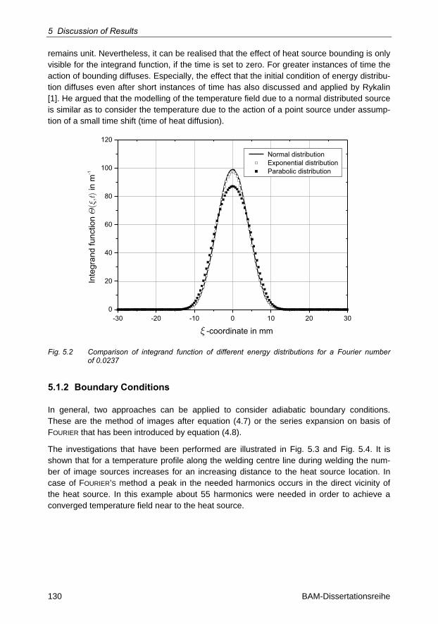
5 Discussion of Results
130 BAM-Dissertationsreihe
remains unit. Nevertheless, it can be realised that the effect of heat source bounding is only visible for the integrand function, if the time is set to zero. For greater instances of time the action of bounding diffuses. Especially, the effect that the initial condition of energy distribu-tion diffuses even after short instances of time has also discussed and applied by Rykalin [1]. He argued that the modelling of the temperature field due to a normal distributed source is similar as to consider the temperature due to the action of a point source under assump-tion of a small time shift (time of heat diffusion).
-30 -20 -10 0 10 20 300
20
40
60
80
100
120
Normal distributionExponential distributionParabolic distribution
� -coordinate in mm
Inte
gran
d fu
nctio
nin
m�
�(,)t
-1
Fig. 5.2 Comparison of integrand function of different energy distributions for a Fourier number of 0.0237
5.1.2 Boundary Conditions
In general, two approaches can be applied to consider adiabatic boundary conditions. These are the method of images after equation (4.7) or the series expansion on basis of FOURIER that has been introduced by equation (4.8).
The investigations that have been performed are illustrated in Fig. 5.3 and Fig. 5.4. It is shown that for a temperature profile along the welding centre line during welding the num-ber of image sources increases for an increasing distance to the heat source location. In case of FOURIER’S method a peak in the needed harmonics occurs in the direct vicinity of the heat source. In this example about 55 harmonics were needed in order to achieve a converged temperature field near to the heat source.
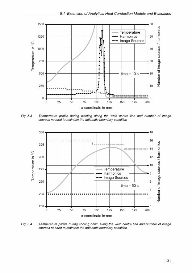
5.1 Extension of Analytical Heat Conduction Models and Evaluation
131
0 25 50 75 100 125 150 175 2000
250
500
750
1000
1250
1500
x-coordinate in mm
0
10
20
30
40
50
60
TemperatureHarmonicsImage Sources
Num
ber o
f im
age
sour
ces
/ har
mon
ics
Tem
pera
ture
in °
C
time = 10 s
Fig. 5.3 Temperature profile during welding along the weld centre line and number of image sources needed to maintain the adiabatic boundary condition
0 25 50 75 100 125 150 175 200200
225
250
275
300
325
350
Tem
pera
ture
in°C
x-coordinate in mm
0
2
4
6
8
10
12
14
16
18
Num
bero
fim
age
sour
ces
/har
mon
ics
TemperatureHarmonicsImage Sources
time = 50 s
Fig. 5.4 Temperature profile during cooling down along the weld centre line and number of image sources needed to maintain the adiabatic boundary condition
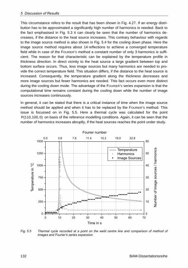
5 Discussion of Results
132 BAM-Dissertationsreihe
This circumstance refers to the result that has been shown in Fig. 4.27. If an energy distri-bution has to be approximated a significantly high number of harmonics is needed. Back to the fact emphasised in Fig. 5.3 it can clearly be seen that the number of harmonics de-creases, if the distance to the heat source increases. This contrary behaviour with regards to the image source method is also shown in Fig. 5.4 for the cooling down phase. Here the image source method requires about 14 reflections to achieve a converged temperature field while in case of the FOURIER’S method a constant number of only 3 harmonics is suffi-cient. The reason for that characteristic can be explained by the temperature profile in thickness direction. In direct vicinity to the heat source a large gradient between top and bottom surface occurs. Thus, less image sources but many harmonics are needed to pro-vide the correct temperature field. This situation differs, if the distance to the heat source is increased. Consequently, the temperature gradient along the thickness decreases and more image sources but fewer harmonics are needed. This fact occurs even more distinct during the cooling down mode. The advantage of the FOURIER’S series expansion is that the computational time remains constant during the cooling down while the number of image sources increases continuously.
In general, it can be stated that there is a critical instance of time when the image source method should be applied and when it has to be replaced by the FOURIER’S method. This issue is focussed on in Fig. 5.5. Here a thermal cycle was calculated for the point P(110,100,0) on basis of the reference modelling conditions. Again, it can be seen that the number of harmonics increases abruptly, if the heat sources reaches the point under study.
0 10 20 30 40 50 60 700
250
500
750
1000
1250
1500
Time in s
0
10
20
30
40
50
600.0 3.8 7.6 11.4 15.2 19.0 22.8
Fourier number
Num
ber o
f im
age
sour
ces
/ har
mon
ics
Tem
pera
ture
in °
C
TemperatureHarmonicsImage Sources
Fig. 5.5 Thermal cycle recorded at a point on the weld centre line and comparison of method of images and Fourier’s series expansion
5.1 Extension of Analytical Heat Conduction Models and Evaluation
133
After that it decreases continuously. The corresponding contrary behaviour is obtained for the method of image sources. To summarise it can be said that for high FOURIER numbers, i.e. for this test case greater than 4.0, FOURIER’S method can be applied and for small FOU-
RIER numbers, here smaller than 4.0, the method of image sources is better suited.
The investigations regarding the performance of the algorithms to consider adiabatic boundaries of the specimen mainly focus on the consideration of the thickness of the plate-like geometry. As discussed previously, the incorporation of side faces requires the same approach but this would increase the computational costs significantly. Because of that the concept of an activation domain was introduced. This means that the computational domain has to be extended by a virtual domain where all the virtually reflected and dummy sources are located. That is the main difference to finite discretisation schemes where the system of equations is only solved for nodes which are located within or at the boundary of the speci-men. The issue also governs the concerns regarding the computational costs of functional-analytical and numerical discretisation approaches. As sketched in Fig. 4.33 the more sub-paths the welding trajectory contains the more dummy sources have to be introduced which are reflected at all bounding surfaces. Therefore, the computational costs are dependent on the complexity of the welding trajectory in the case of functional-analytical methods. This is obviously not the case, if numerical methods are taken.
The concept of an activation domain allows reducing the computational cost significantly. This method is especially suitable for the reflections with respect to the side faces of the specimen since the dimension in width and length direction is higher than in thickness direc-tion. Because of that fact many reflections or harmonics are needed in thickness direction while mostly only one reflection has to be used for the side faces which can then be even neglected by application of the activation range. Of course, these assumptions can not be made for the cooling down phase since the heat diffusion of heat sources which do not affect the temperature field in the computational domain during welding can now influence that domain during the cooling down phase. Thus, a further requirement of the concept of activation range is that if the real heat source stops acting all reflected heat sources are activated.
To summarize the concept of a virtual computation domain is a consequence of the funda-mental functional-analytical solutions which are defined for the infinite solid. The bounding faces can be incorporated by usage of the image or FOURIER’S method. The series are trun-cated, if a temperature convergence criterion of 1 x 10⁻⁵ is reached. Nevertheless, at least one reflection is needed in order to evaluate this convergence criterion. While in the case of the series expansion in thickness direction this fact has no important meaning since many reflections/harmonics have to be applied this situation changes for the side faces as heat impermeable boundaries. Here, even a single reflection would increase the computational costs significantly. To overcome this problem the concept of an activation range is intro-duced to neglect those heat sources having no influence on the temperature field in the computational domain yet.
5.1.3 Movement on Curved Trajectories
The objective of this test case was to evaluate to what extent the introduction of the three dimensional velocity vector as proposed by equation (4.44) enables to model the movement
5 Discussion of Results
134 BAM-Dissertationsreihe
of symmetrically and asymmetrically distributed heat sources along arbitrary oriented weld paths or if this can only be solved by a coordinate transformation. The concept of the direct introduction of the velocity vector was also followed by Cao [123] and Winczek [124].
The basic approach of modelling the movement on curved trajectories is outlined in chap-ter 4.2.2.3. The idea is based on the decomposition of the welding trajectory into linear sub-paths which have a certain orientation with respect to the global coordinate system. There-fore, the corresponding test case investigated the movement of a double ellipsoidal as well as a spherical heat source on a sub path parallel and inclined to the global x -axis. It is shown in Fig. 4.34 - Fig. 4.36 that the direct application of the velocity vector in terms of the global reference frame yields, in case of the spherical heat source, the same results as if a coordinate transformation is employed. However, the situation is different for the double ellipsoidal heat source as illustrated in Fig. 4.35 a) and Fig. 4.36. If only global coordinates are considered by direct usage of the velocity vector the resulting temperature field is de-generated. This is because the energy distribution parameters are defined with respect to the local coordinate system that is aligned with the heat source. The energy distribution parameters should be recalculated in dependence on the orientation of the current sub path under study.
Because this is not a trivial task to be performed in terms of global coordinates, the concept of coordinate transformation that includes a translation and rotation was implemented. It can be shown that this approach yields the correct temperature field for volume heat sources that move on arbitrary oriented welding trajectories. This not only holds for the asymmetric definition of the energy distribution but also for the boundary of the heat source action since it is defined with respect to the local coordinate system (Fig. 3.5). Concluding it can be remarked that the global approach after Cao [123] only works for concentrated or symmetrically distributed heat sources [124]. The approach that is presented here is inde-pendent on the energy distribution and can be applied for arbitrary shaped and bounded volume heat sources. Furthermore, it is worth noticing that the concept of the coordinate transformation allows the direct application of the equation framework that was presented in chapter 4.2.1. The calculation of the temperature field for a virtual sub-path that enables the consideration of heat impermeable boundaries can easily be formulated in terms of the variables ( )x y z0 0 0, , which describe the distance of the heat source origin to the bound-ing faces under consideration of the corresponding length measures ( )x y zL L L, , . The real orientation of the heat source is then taken into account by a translation and rotation as outlined in equation (4.48) and (4.50).
5.1.4 Comparison with Finite Element Model
The introduced functional-analytical framework is compared with finite element models that obey temperature independent thermo-physical material properties. This allows evaluating the influence of the spatial and temporal discretisation of finite element models. On the other hand, the implementation of the movement of distributed heat sources, e.g. double ellipsoidal ones, on curved trajectories on basis of functional-analytical methods can be validated because no analytical references are available in literature.
As explained in chapter 3.2.2.5 (page 42) the comparison involves the movement on a trajectory with sub-paths that have an arbitrary orientation with respect to the global coordi-
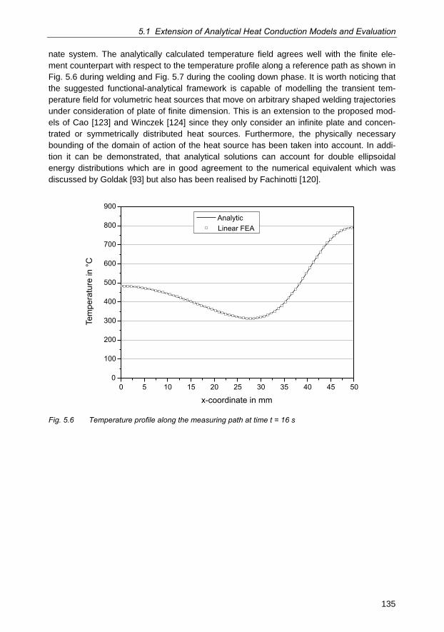
5.1 Extension of Analytical Heat Conduction Models and Evaluation
135
nate system. The analytically calculated temperature field agrees well with the finite ele-ment counterpart with respect to the temperature profile along a reference path as shown in Fig. 5.6 during welding and Fig. 5.7 during the cooling down phase. It is worth noticing that the suggested functional-analytical framework is capable of modelling the transient tem-perature field for volumetric heat sources that move on arbitrary shaped welding trajectories under consideration of plate of finite dimension. This is an extension to the proposed mod-els of Cao [123] and Winczek [124] since they only consider an infinite plate and concen-trated or symmetrically distributed heat sources. Furthermore, the physically necessary bounding of the domain of action of the heat source has been taken into account. In addi-tion it can be demonstrated, that analytical solutions can account for double ellipsoidal energy distributions which are in good agreement to the numerical equivalent which was discussed by Goldak [93] but also has been realised by Fachinotti [120].
0
100
200
300
400
500
600
700
800
900
0 5 10 15 20 25 30 35 40 45 50
x-coordinate in mm
AnalyticLinear FEA
Tem
pera
ture
in °
C
Fig. 5.6 Temperature profile along the measuring path at time t = 16 s
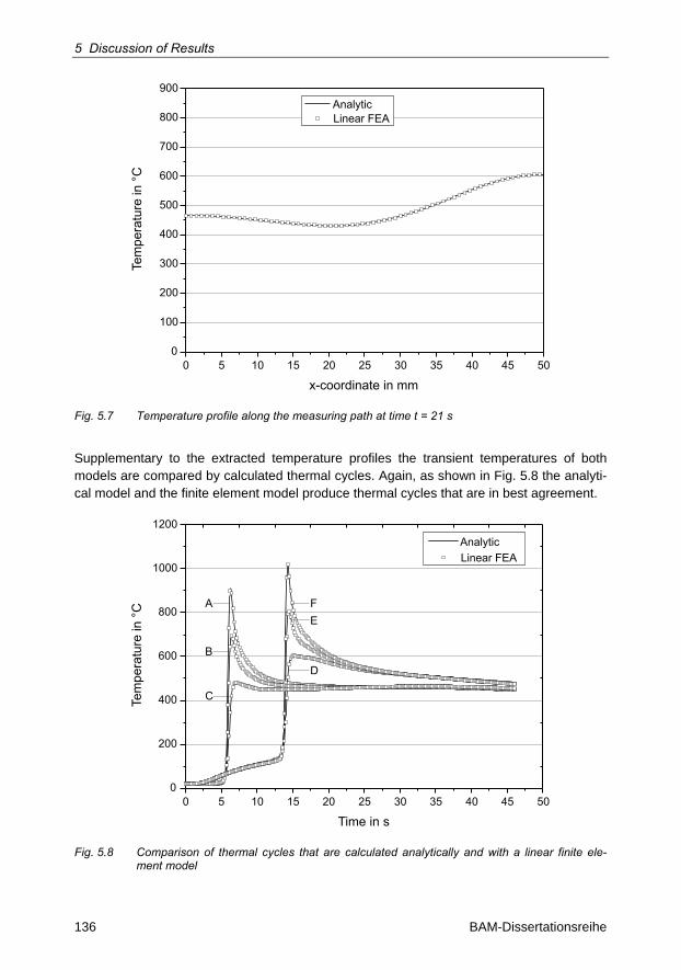
5 Discussion of Results
136 BAM-Dissertationsreihe
0
100
200
300
400
500
600
700
800
900AnalyticLinear FEA
0 5 10 15 20 25 30 35 40 45 50
x-coordinate in mm
Tem
pera
ture
in °
C
Fig. 5.7 Temperature profile along the measuring path at time t = 21 s
Supplementary to the extracted temperature profiles the transient temperatures of both models are compared by calculated thermal cycles. Again, as shown in Fig. 5.8 the analyti-cal model and the finite element model produce thermal cycles that are in best agreement.
0 5 10 15 20 25 30 35 40 45 500
200
400
600
800
1000
1200
Time in s
AnalyticLinear FEA
Tem
pera
ture
in °
C A
B
C
FE
D
Fig. 5.8 Comparison of thermal cycles that are calculated analytically and with a linear finite ele-ment model
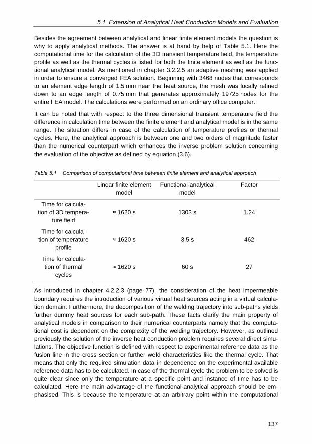
5.1 Extension of Analytical Heat Conduction Models and Evaluation
137
Besides the agreement between analytical and linear finite element models the question is why to apply analytical methods. The answer is at hand by help of Table 5.1. Here the computational time for the calculation of the 3D transient temperature field, the temperature profile as well as the thermal cycles is listed for both the finite element as well as the func-tional analytical model. As mentioned in chapter 3.2.2.5 an adaptive meshing was applied in order to ensure a converged FEA solution. Beginning with 3468 nodes that corresponds to an element edge length of 1.5 mm near the heat source, the mesh was locally refined down to an edge length of 0.75 mm that generates approximately 19725 nodes for the entire FEA model. The calculations were performed on an ordinary office computer.
It can be noted that with respect to the three dimensional transient temperature field the difference in calculation time between the finite element and analytical model is in the same range. The situation differs in case of the calculation of temperature profiles or thermal cycles. Here, the analytical approach is between one and two orders of magnitude faster than the numerical counterpart which enhances the inverse problem solution concerning the evaluation of the objective as defined by equation (3.6).
Table 5.1 Comparison of computational time between finite element and analytical approach
Linear finite element model
Functional-analytical model
Factor
Time for calcula-tion of 3D tempera-
ture field ≈ 1620 s 1303 s 1.24
Time for calcula-tion of temperature
profile ≈ 1620 s 3.5 s 462
Time for calcula-tion of thermal
cycles ≈ 1620 s 60 s 27
As introduced in chapter 4.2.2.3 (page 77), the consideration of the heat impermeable boundary requires the introduction of various virtual heat sources acting in a virtual calcula-tion domain. Furthermore, the decomposition of the welding trajectory into sub-paths yields further dummy heat sources for each sub-path. These facts clarify the main property of analytical models in comparison to their numerical counterparts namely that the computa-tional cost is dependent on the complexity of the welding trajectory. However, as outlined previously the solution of the inverse heat conduction problem requires several direct simu-lations. The objective function is defined with respect to experimental reference data as the fusion line in the cross section or further weld characteristics like the thermal cycle. That means that only the required simulation data in dependence on the experimental available reference data has to be calculated. In case of the thermal cycle the problem to be solved is quite clear since only the temperature at a specific point and instance of time has to be calculated. Here the main advantage of the functional-analytical approach should be em-phasised. This is because the temperature at an arbitrary point within the computational
5 Discussion of Results
138 BAM-Dissertationsreihe
domain and specific time can be calculated independently on neighbouring points/locations and previous instances of time. In case of a numerical method, as finite element analysis, the situation is different since the influence of neighbouring points/nodes is defined by the composition of the global stiffness matrix of the system under consideration and the ele-ment connectivity [189]. In other words, the complete system of equations needs to be solved for every node and every time step in order to get information of the dependent variable at a specific location. If this location is not coinciding with a node, or more precisely GAUSS -point of the discretised system, then the shape function of the element has to be used to evaluate the (interpolated) value of temperature at a specific point. It can be easily seen that the evaluation of temperature is orders of magnitudes faster, if a functional-analytical method is used than a numerical approach. However, the increase in speed re-sults in a reduction of model complexity like the neglect of the temperature dependence of the material properties. The presentation of the algorithm in Fig. 4.43 showed that only a few evaluations of temperatures at specific points are needed to reconstruct the fusion line in the cross section. Of course, the same algorithm could be applied for a numerical model to extract the geometry of the fusion line out of the calculated 3D temperature field. In this case, for every search point the corresponding temperature values have to be interpolated from the nearest GAUSS-points by means of the element shape functions. This requires having the 3D temperature field at a certain instance of time available which, as already discussed, includes the solution of the system of equations for all nodes and previous time steps. Again, the advantage of functional-analytical methods is clarified by fulfilling the same task orders of magnitudes faster.
5.2 Solution of the Inverse Heat Conduction Problem
The core capability of a simulation environment whose task is to solve the inverse heat conduction problem is governed by the presence of a fast and reliable temperature field calculation. In particular, the computational correspondence to experimental reference data like fusion line in the cross section and weld pool geometry characteristics as well as thermo couple measurements has to be provided by the simulation framework. Thus, the subsequent discussions focus on solving the objective functional as e.g. presented by equation (2.9) or (3.6) with basis on the fusion line, weld pool length at the top surface and thermal cycle measurements at the top and bottom surface.
5.2.1 Sensitivity of Heat Source Models
The solution of the inverse heat conduction problem involves the evaluation of those input parameters of the model so that the corresponding simulation result is in optimal agreement with the experimental reference data. Besides the application of sophisticated optimisation algorithms that are based on local or global search techniques as well as the combination of both approaches one main aspect has to be kept in mind. This is related to the dimen-sion of the model parameter space under study. The functional-analytical simulation frame-work that is presented here includes the definition of the boundary and the heat source distribution as direct model input parameters. In case of a double ellipsoidal heat source the model parameter space involves 11 dimensions, 6 for the boundary of heat source action, 4 distribution parameters and the heat input. If each dimension would only be discretised into
5.2 Solution of the Inverse Heat Conduction Problem
139
10 sub-intervals it increases the total quantity of the search space to 1011 elements. This is an amount of data points, where a structured search is impossible. Therefore, the knowl-edge about the general sensitivity of the model with respect to the variation of its input pa-rameters is important in order to detect the efficiency of model parameters regarding the calibration behaviour and to localise regions where it is worthwhile to search for the global minimum.
In Fig. 4.44 - Fig. 4.47 (page 94- 96) the sensitivity of the weld pool characteristics top width, bottom width, weld pool length and penetration depth was studied for a two dimen-sional model parameter space. Even though this does not correspond to the most arbitrary case, given of a bounded double ellipsoidal heat source, the general behaviour of volume heat sources can be explored. Another fact that needs to be mentioned is that the pre-sented contour plots are based on matrices with a dimension 160 x 160. Consequently, 25600 direct simulations are needed in order to evaluate the global sensitivity behaviour of the heat source model under study. In case of analytical models this number of simulations is not a problem and requires approximately 15 – 30 minutes on an ordinary office com-puter. On the other hand, the same investigation would not have been possible by applica-tion of numerical modelling paradigms, e.g. finite element method. Thus, the benefit of functional-analytical methods is also based on the fact that they allow very efficient and detailed analyses of the general behaviour of volumetrically distributed heat source models. The obtained conclusions are also applicable for heat conduction models that consider more complex geometries or are based on numerical methods. Therefore, the presented results can be treated as fundamental concerning the efficient solution of the inverse heat conduction problem.
With respect to the dimension of the weld pool a typical characteristic of volumetric energy distributions occurs. This is given by the relationship between a pool characteristic and a certain energy distribution parameter. It can exemplarily be seen for the top weld pool width in Fig. 4.44, page 94. If the energy distribution parameter ez is kept constant, say zero, then the pool width at the top surface increases, if the parameter e xyr , is increased. The relationship only holds up to a value of e xyr , = 6.5mm and is then inverted. This means a further increase of e xyr , now yields a decrease of the top weld pool width. It is clear that this happens because the energy intensity decreases, if e xyr , increases. With respect to the molten region at the top surface it can be concluded that for the parameter e xyr , the maxi-mum width of the molten zone is obtained at e xyr , » 5.3mm and not at the point of highest intensity distribution, which is e xyr , » 0 and ez » 0 . This result coincides with those of Rykalin [1]. However, it has to be noted that the behaviour is different, if the parameter
e e e eR x h z= = = is varied, which is illustrated in Fig. 5.9. Therefore, in case of a spheri-cal distributed heat source the maximum melting at the top surface occurs for the highest energy intensity that is obtained if eR tends to zero.
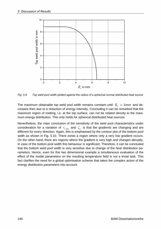
5 Discussion of Results
140 BAM-Dissertationsreihe
0 2 4 6 8 100
2
4
6
8
10
Re in mm
Top
wel
d po
ol w
idth
in m
m
Fig. 5.9 Top weld pool width plotted against the radius of a spherical normal distributed heat source
The maximum obtainable top weld pool width remains constant until eR » 3mm and de-creases then due to a reduction of energy intensity. Concluding it can be remarked that the maximum region of melting, i.e. at the top surface, can not be related directly to the maxi-mum energy distribution. This only holds for spherical distributed heat sources.
Nevertheless, the main conclusion of the sensitivity of the weld pool characteristics under consideration for a variation of e xyr , and ez is that the gradients are changing and are different for every direction. Again, this is emphasised by the contour plot of the bottom pool width as shown in Fig. 5.10. There exists a region where only a very low gradient occurs. On the other hand, there are regions where the gradient is very high and changes abruptly. In case of the bottom pool width this behaviour is significant. Therefore, it can be concluded that the bottom weld pool width is very sensitive due to change of the heat distribution pa-rameters. Hence, even for this two dimensional example a simultaneous evaluation of the effect of the model parameters on the resulting temperature field is not a trivial task. This fact clarifies the need for a global optimisation scheme that takes the complex action of the energy distribution parameters into account.
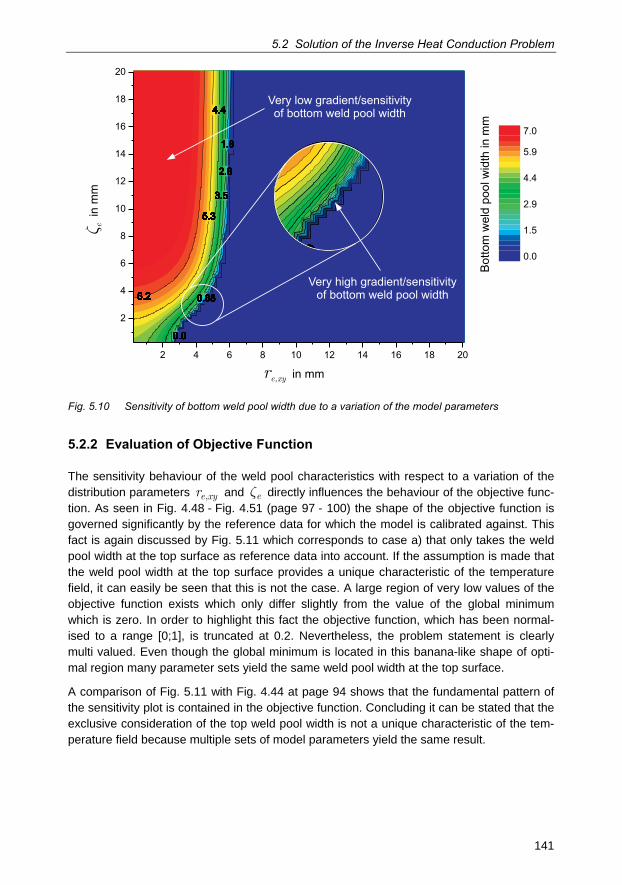
5.2 Solution of the Inverse Heat Conduction Problem
141
Bot
tom
wel
d po
ol w
idth
in m
m
6.2
5.3
4.4
3.5
2.6
1.8
0.88
0.0
6.2
5.3
4.4
3.5
2.6
1.8
0.88
0.0
6.2
5.3
4.4
3.5
2.6
1.8
0.88
0.0
6.2
5.3
4.4
3.5
2.6
1.8
0.88
0.0
6.2
5.3
4.4
3.5
2.6
1.8
0.88
0.0
6.2
5.3
4.4
3.5
2.6
1.8
0.88
0.0
6.2
5.3
4.4
3.5
2.6
1.8
0.88
0.0
6.2
5.3
4.4
3.5
2.6
1.8
0.88
0.0
6.2
5.3
4.4
3.5
2.6
1.8
0.88
0.0
6.2
5.3
4.4
3.5
2.6
1.8
0.88
0.0
6.2
5.3
4.4
3.5
2.6
1.8
0.88
0.0
6.2
5.3
4.4
3.5
2.6
1.8
0.88
0.0
6.2
5.3
4.4
3.5
2.6
1.8
0.88
0.0
6.2
5.3
4.4
3.5
2.6
1.8
0.88
0.0
6.2
5.3
4.4
3.5
2.6
1.8
0.88
0.0
6.2
5.3
4.4
3.5
2.6
1.8
0.88
0.0
6.2
5.3
4.4
3.5
2.6
1.8
0.88
0.0
6.2
5.3
4.4
3.5
2.6
1.8
0.88
0.0
6.2
5.3
4.4
3.5
2.6
1.8
0.88
0.0
6.2
5.3
4.4
3.5
2.6
1.8
0.88
0.0
6.2
5.3
4.4
3.5
2.6
1.8
0.88
0.0
6.2
5.3
4.4
3.5
2.6
1.8
0.88
0.0
6.2
5.3
4.4
3.5
2.6
1.8
0.88
0.0
6.2
5.3
4.4
3.5
2.6
1.8
0.88
0.0
6.2
5.3
4.4
3.5
2.6
1.8
0.88
0.0
6.2
5.3
4.4
3.5
2.6
1.8
0.88
0.0
6.2
5.3
4.4
3.5
2.6
1.8
0.88
0.0
6.2
5.3
4.4
3.5
2.6
1.8
0.88
0.0
6.2
5.3
4.4
3.5
2.6
1.8
0.88
0.0
6.2
5.3
4.4
3.5
2.6
1.8
0.88
0.0
6.2
5.3
4.4
3.5
2.6
1.8
0.88
0.0
6.2
5.3
4.4
3.5
2.6
1.8
0.88
0.0
6.2
5.3
4.4
3.5
2.6
1.8
0.88
0.0
6.2
5.3
4.4
3.5
2.6
1.8
0.88
0.0
6.2
5.3
4.4
3.5
2.6
1.8
0.88
0.0
6.2
5.3
4.4
3.5
2.6
1.8
0.88
0.0
6.2
5.3
4.4
3.5
2.6
1.8
0.88
0.0
6.2
5.3
4.4
3.5
2.6
1.8
0.88
0.0
6.2
5.3
4.4
3.5
2.6
1.8
0.88
0.0
6.2
5.3
4.4
3.5
2.6
1.8
0.88
0.0
6.2
5.3
4.4
3.5
2.6
1.8
0.88
0.0
6.2
5.3
4.4
3.5
2.6
1.8
0.88
0.0
6.2
5.3
4.4
3.5
2.6
1.8
0.88
0.0
6.2
5.3
4.4
3.5
2.6
1.8
0.88
0.0
6.2
5.3
4.4
3.5
2.6
1.8
0.88
0.0
6.2
5.3
4.4
3.5
2.6
1.8
0.88
0.0
6.2
5.3
4.4
3.5
2.6
1.8
0.88
0.0
6.2
5.3
4.4
3.5
2.6
1.8
0.88
0.0
6.2
5.3
4.4
3.5
2.6
1.8
0.88
0.0
6.2
5.3
4.4
3.5
2.6
1.8
0.88
0.0
6.2
5.3
4.4
3.5
2.6
1.8
0.88
0.0
2 4 6 8 10 12 14 16 18 20
2
4
6
8
10
12
14
16
18
20
0.0
1.5
2.9
4.4
5.9
7.0
Very high gradient/sensitivityof bottom weld pool width
Very low gradient/sensitivityof bottom weld pool width
re,xy in mm
� ein
mm
Fig. 5.10 Sensitivity of bottom weld pool width due to a variation of the model parameters
5.2.2 Evaluation of Objective Function
The sensitivity behaviour of the weld pool characteristics with respect to a variation of the distribution parameters e xyr , and ez directly influences the behaviour of the objective func-tion. As seen in Fig. 4.48 - Fig. 4.51 (page 97 - 100) the shape of the objective function is governed significantly by the reference data for which the model is calibrated against. This fact is again discussed by Fig. 5.11 which corresponds to case a) that only takes the weld pool width at the top surface as reference data into account. If the assumption is made that the weld pool width at the top surface provides a unique characteristic of the temperature field, it can easily be seen that this is not the case. A large region of very low values of the objective function exists which only differ slightly from the value of the global minimum which is zero. In order to highlight this fact the objective function, which has been normal-ised to a range [0;1], is truncated at 0.2. Nevertheless, the problem statement is clearly multi valued. Even though the global minimum is located in this banana-like shape of opti-mal region many parameter sets yield the same weld pool width at the top surface.
A comparison of Fig. 5.11 with Fig. 4.44 at page 94 shows that the fundamental pattern of the sensitivity plot is contained in the objective function. Concluding it can be stated that the exclusive consideration of the top weld pool width is not a unique characteristic of the tem-perature field because multiple sets of model parameters yield the same result.
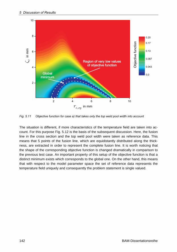
5 Discussion of Results
142 BAM-Dissertationsreihe
2 4 6 8 10
2
4
6
8
10
Globalminimum
Globalminimum
Region of very low valuesof objective function
Region of very low valuesof objective function
0,0
0.043
0.087
0.13
0.17
0.20
Obj
ectiv
e fu
nctio
n
re,xy in mm
� ein
mm
Fig. 5.11 Objective function for case a) that takes only the top weld pool width into account
The situation is different, if more characteristics of the temperature field are taken into ac-count. For this purpose Fig. 5.12 is the basis of the subsequent discussion. Here, the fusion line in the cross section and the top weld pool width were taken as reference data. This means that 5 points of the fusion line, which are equidistantly distributed along the thick-ness, are extracted in order to represent the complete fusion line. It is worth noticing that the shape of the corresponding objective function is changed dramatically in comparison to the previous test case. An important property of this setup of the objective function is that a distinct minimum exists which corresponds to the global one. On the other hand, this means that with respect to the model parameter space the set of reference data represents the temperature field uniquely and consequently the problem statement is single valued.
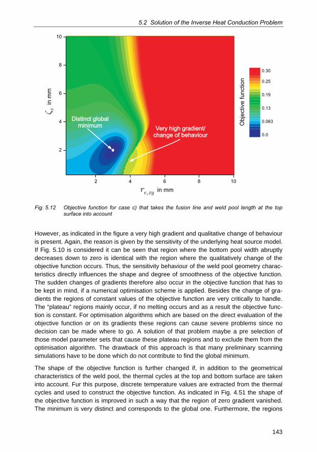
5.2 Solution of the Inverse Heat Conduction Problem
143
2 4 6 8 10
2
4
6
8
10
Distinct globalminimum
Distinct globalminimum Very high gradient/
change of behaviourVery high gradient/
change of behaviour 0.0
0.063
0.13
0.19
0.25
0.30
Obj
ectiv
e fu
nctio
n
re,xy in mm
� ein
mm
Fig. 5.12 Objective function for case c) that takes the fusion line and weld pool length at the top surface into account
However, as indicated in the figure a very high gradient and qualitative change of behaviour is present. Again, the reason is given by the sensitivity of the underlying heat source model. If Fig. 5.10 is considered it can be seen that region where the bottom pool width abruptly decreases down to zero is identical with the region where the qualitatively change of the objective function occurs. Thus, the sensitivity behaviour of the weld pool geometry charac-teristics directly influences the shape and degree of smoothness of the objective function. The sudden changes of gradients therefore also occur in the objective function that has to be kept in mind, if a numerical optimisation scheme is applied. Besides the change of gra-dients the regions of constant values of the objective function are very critically to handle. The “plateau” regions mainly occur, if no melting occurs and as a result the objective func-tion is constant. For optimisation algorithms which are based on the direct evaluation of the objective function or on its gradients these regions can cause severe problems since no decision can be made where to go. A solution of that problem maybe a pre selection of those model parameter sets that cause these plateau regions and to exclude them from the optimisation algorithm. The drawback of this approach is that many preliminary scanning simulations have to be done which do not contribute to find the global minimum.
The shape of the objective function is further changed if, in addition to the geometrical characteristics of the weld pool, the thermal cycles at the top and bottom surface are taken into account. Fur this purpose, discrete temperature values are extracted from the thermal cycles and used to construct the objective function. As indicated in Fig. 4.51 the shape of the objective function is improved in such a way that the region of zero gradient vanished. The minimum is very distinct and corresponds to the global one. Furthermore, the regions
5 Discussion of Results
144 BAM-Dissertationsreihe
of very high gradients and change of behaviour are also reduced significantly. In total, the shape of the objective function is very suitable for the application of optimisation algorithms because it is very smooth. Nevertheless, one issue has to be emphasised here. If the objec-tive function is constructed after equation (3.6) the magnitudes of the reference data should have the same order. If only the weld pool characteristics are taken into account this re-quirement is ensured. The situation changes, if the temperature values are added since they obey greater numerical values if the units are set in accordance to international system of units. In this case, the shape of the objective function would be over predicted by the temperature information. To avoid this behaviour an appropriate normalisation of each reference quantity has to be made or the corresponding weight in the objective function has to be reduced. The application of the weighting coefficients in the objective function is also reasonable, if a certain temperature field quantity has a very high sensitivity. This is exem-plary the case for the bottom weld pool width. Thus, in order to smooth the shape of the objective function the corresponding weight may be reduced. However, if the weights of the objective function are adjusted it always has to be guaranteed that the information of the included temperature field characteristics is not lost and that still a distinct global minimum exists.
To summarise it can be concluded that the knowledge about the sensitivity and the result-ing shape of the objective function enables to characterise the applicability of optimisation algorithms. The main requirement that has to be met is the existence of a distinct global minimum. It could be shown that this property is dependent of the reference data that is taken into account. For the test case under study, the fusion line in the cross section, the top weld pool length as well as the thermal cycles enables to create a smooth objective function with a distinct global minimum. However, the investigation of the shape of the ob-jective functions becomes complicated if model parameter spaces of higher dimension are of interest since the shape of the objective function corresponds to a hyper surface. Never-theless, it can be stated that since for the two dimensional model parameter spaces at least the fusion line in the cross section, weld pool length and thermal cycles are needed as reference data in order to setup an appropriate objective function the amount of required temperature field characteristics cannot be reduced for the multi dimensional cases. Be-cause it is too time consuming even for analytical methods to explore the shape of the ob-jective function by structured scanning simulations as applied for the two dimensional case, a method of evaluating the presence of a distinct global minimum on basis of artificial intel-ligence is presented for a three dimensional parameter space in the subsequent chapter.
5.2.3 Calibration Behaviour of Heat Source Models
In the previous chapter the shape of the objective function was discussed and served as criterion for the evaluation of the applicability of optimisation routines. The objective of this section is to discuss the usability of a neural network based optimisation routine to solve the inverse heat conduction problem for a two and three dimensional model parameter space. As mentioned, a structured scanning of the parameter space is even limited in case of ana-lytical methods since many direct simulations are needed. With reference to chapter 3.2.3.3 (page 45) it has to be noted that objective functions for the two dimensional problem pre-sented above required 160 x 160 = 25 600 simulations runs. The number of simulations maybe solvable by an analytical method because the computational time was only 15 –
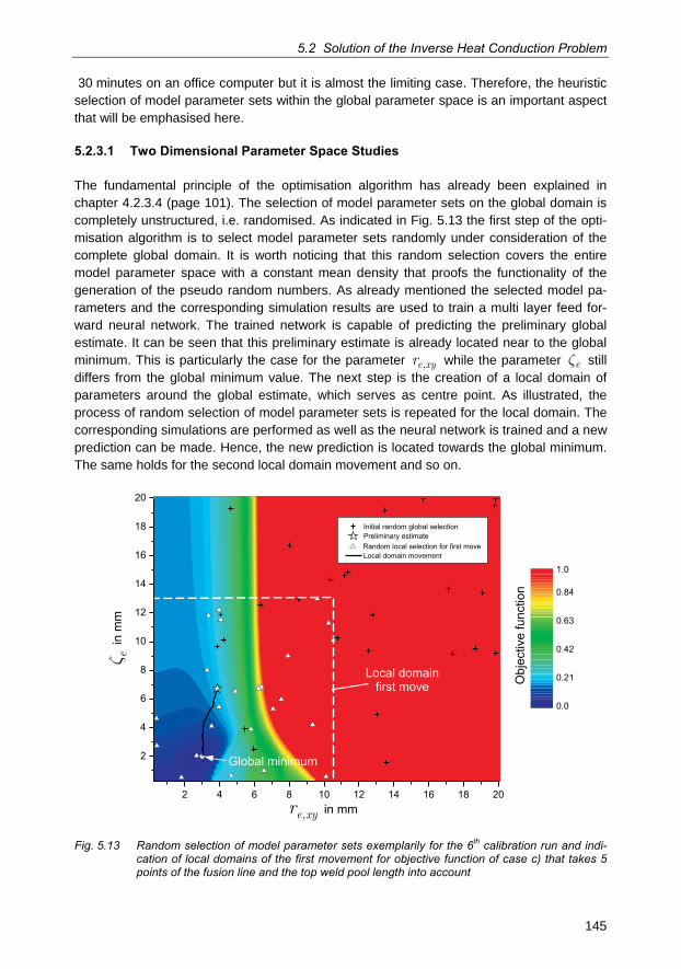
5.2 Solution of the Inverse Heat Conduction Problem
145
30 minutes on an office computer but it is almost the limiting case. Therefore, the heuristic selection of model parameter sets within the global parameter space is an important aspect that will be emphasised here.
5.2.3.1 Two Dimensional Parameter Space Studies
The fundamental principle of the optimisation algorithm has already been explained in chapter 4.2.3.4 (page 101). The selection of model parameter sets on the global domain is completely unstructured, i.e. randomised. As indicated in Fig. 5.13 the first step of the opti-misation algorithm is to select model parameter sets randomly under consideration of the complete global domain. It is worth noticing that this random selection covers the entire model parameter space with a constant mean density that proofs the functionality of the generation of the pseudo random numbers. As already mentioned the selected model pa-rameters and the corresponding simulation results are used to train a multi layer feed for-ward neural network. The trained network is capable of predicting the preliminary global estimate. It can be seen that this preliminary estimate is already located near to the global minimum. This is particularly the case for the parameter e xyr , while the parameter ez still differs from the global minimum value. The next step is the creation of a local domain of parameters around the global estimate, which serves as centre point. As illustrated, the process of random selection of model parameter sets is repeated for the local domain. The corresponding simulations are performed as well as the neural network is trained and a new prediction can be made. Hence, the new prediction is located towards the global minimum. The same holds for the second local domain movement and so on.
2 4 6 8 10 12 14 16 18 20
2
4
6
8
10
12
14
16
18
20
Obj
ectiv
efu
nctio
n
0.0
0.21
0.42
0.63
0.84
1.0
Initial random global selection
Local domain movement
Preliminary estimateRandom local selection for first move
Local domainfirst move
Global minimum
re,xy in mm
� ein
mm
Fig. 5.13 Random selection of model parameter sets exemplarily for the 6th calibration run and indi-cation of local domains of the first movement for objective function of case c) that takes 5 points of the fusion line and the top weld pool length into account
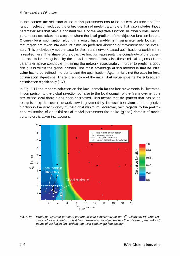
5 Discussion of Results
146 BAM-Dissertationsreihe
In this context the selection of the model parameters has to be noticed. As indicated, the random selection includes the entire domain of model parameters that also includes those parameter sets that yield a constant value of the objective function. In other words, model parameters are taken into account where the local gradient of the objective function is zero. Ordinary local optimisation algorithms would have problems, if parameter sets located in that region are taken into account since no preferred direction of movement can be evalu-ated. This is obviously not the case for the neural network based optimisation algorithm that is applied here. The shape of the objective function represents the complexity of the pattern that has to be recognised by the neural network. Thus, also these critical regions of the parameter space contribute in training the network appropriately in order to predict a good first guess within the global domain. The main advantage of this method is that no initial value has to be defined in order to start the optimisation. Again, this is not the case for local optimisation algorithms. There, the choice of the initial start value governs the subsequent optimisation significantly [169].
In Fig. 5.14 the random selection on the local domain for the last movements is illustrated. In comparison to the global selection but also to the local domain of the first movement the size of the local domain has been decreased. This means that the pattern that has to be recognised by the neural network now is governed by the local behaviour of the objective function in the direct vicinity of the global minimum. Moreover, with regards to the prelimi-nary estimation of an initial set of model parameters the entire (global) domain of model parameters is taken into account.
2 4 6 8 10 12 14 16 18 20
2
4
6
8
10
12
14
16
18
20
Obj
ectiv
efu
nctio
n
0.0
0.21
0.42
0.63
0.84
1.0
Initial random global selection
Local domain movementPreliminary estimate
Random local selection for last move
Global minimum
Local domainlast move
re,xy in mm
� ein
mm
Fig. 5.14 Random selection of model parameter sets exemplarily for the 6th calibration run and indi-cation of local domains of last two movements for objective function of case c) that takes 5 points of the fusion line and the top weld pool length into account
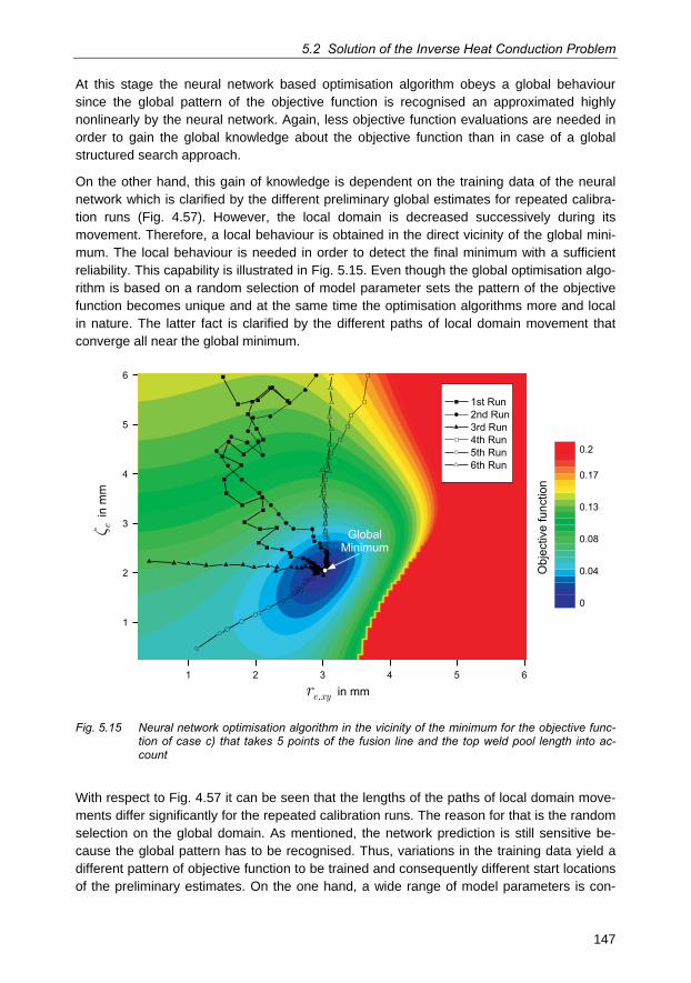
5.2 Solution of the Inverse Heat Conduction Problem
147
At this stage the neural network based optimisation algorithm obeys a global behaviour since the global pattern of the objective function is recognised an approximated highly nonlinearly by the neural network. Again, less objective function evaluations are needed in order to gain the global knowledge about the objective function than in case of a global structured search approach.
On the other hand, this gain of knowledge is dependent on the training data of the neural network which is clarified by the different preliminary global estimates for repeated calibra-tion runs (Fig. 4.57). However, the local domain is decreased successively during its movement. Therefore, a local behaviour is obtained in the direct vicinity of the global mini-mum. The local behaviour is needed in order to detect the final minimum with a sufficient reliability. This capability is illustrated in Fig. 5.15. Even though the global optimisation algo-rithm is based on a random selection of model parameter sets the pattern of the objective function becomes unique and at the same time the optimisation algorithms more and local in nature. The latter fact is clarified by the different paths of local domain movement that converge all near the global minimum.
1 2 3 4 5 6
1
2
3
4
5
6
0
0.04
0.08
0.13
0.17
0.2
1st Run2nd Run3rd Run4th Run5th Run6th Run
re,xy in mm
� ein
mm
Obj
ectiv
e fu
nctio
nGlobal
Minimum
Fig. 5.15 Neural network optimisation algorithm in the vicinity of the minimum for the objective func-tion of case c) that takes 5 points of the fusion line and the top weld pool length into ac-count
With respect to Fig. 4.57 it can be seen that the lengths of the paths of local domain move-ments differ significantly for the repeated calibration runs. The reason for that is the random selection on the global domain. As mentioned, the network prediction is still sensitive be-cause the global pattern has to be recognised. Thus, variations in the training data yield a different pattern of objective function to be trained and consequently different start locations of the preliminary estimates. On the one hand, a wide range of model parameters is con-
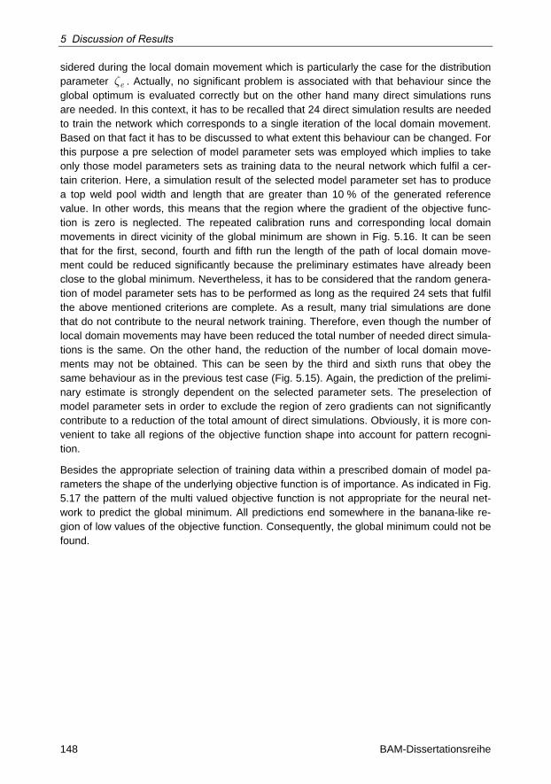
5 Discussion of Results
148 BAM-Dissertationsreihe
sidered during the local domain movement which is particularly the case for the distribution parameter ez . Actually, no significant problem is associated with that behaviour since the global optimum is evaluated correctly but on the other hand many direct simulations runs are needed. In this context, it has to be recalled that 24 direct simulation results are needed to train the network which corresponds to a single iteration of the local domain movement. Based on that fact it has to be discussed to what extent this behaviour can be changed. For this purpose a pre selection of model parameter sets was employed which implies to take only those model parameters sets as training data to the neural network which fulfil a cer-tain criterion. Here, a simulation result of the selected model parameter set has to produce a top weld pool width and length that are greater than 10 % of the generated reference value. In other words, this means that the region where the gradient of the objective func-tion is zero is neglected. The repeated calibration runs and corresponding local domain movements in direct vicinity of the global minimum are shown in Fig. 5.16. It can be seen that for the first, second, fourth and fifth run the length of the path of local domain move-ment could be reduced significantly because the preliminary estimates have already been close to the global minimum. Nevertheless, it has to be considered that the random genera-tion of model parameter sets has to be performed as long as the required 24 sets that fulfil the above mentioned criterions are complete. As a result, many trial simulations are done that do not contribute to the neural network training. Therefore, even though the number of local domain movements may have been reduced the total number of needed direct simula-tions is the same. On the other hand, the reduction of the number of local domain move-ments may not be obtained. This can be seen by the third and sixth runs that obey the same behaviour as in the previous test case (Fig. 5.15). Again, the prediction of the prelimi-nary estimate is strongly dependent on the selected parameter sets. The preselection of model parameter sets in order to exclude the region of zero gradients can not significantly contribute to a reduction of the total amount of direct simulations. Obviously, it is more con-venient to take all regions of the objective function shape into account for pattern recogni-tion.
Besides the appropriate selection of training data within a prescribed domain of model pa-rameters the shape of the underlying objective function is of importance. As indicated in Fig. 5.17 the pattern of the multi valued objective function is not appropriate for the neural net-work to predict the global minimum. All predictions end somewhere in the banana-like re-gion of low values of the objective function. Consequently, the global minimum could not be found.
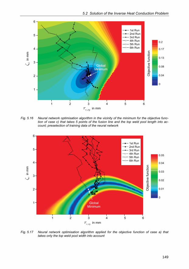
5.2 Solution of the Inverse Heat Conduction Problem
149
1 2 3 4 5 6
1
2
3
4
5
6
1st Run2nd Run3rd Run4th Run5th Run6th Run
re,xy in mm
� ein
mm
GlobalMinimum
0
0.04
0.08
0.13
0.17
0.2
Obj
ectiv
e fu
nctio
n
Fig. 5.16 Neural network optimisation algorithm in the vicinity of the minimum for the objective func-tion of case c) that takes 5 points of the fusion line and the top weld pool length into ac-count; preselection of training data of the neural network
0
0.01
0.02
0.03
0.04
0.05
Obj
ectiv
e fu
nctio
n
GlobalMinimum
1st Run2nd Run3rd Run4th Run5th Run6th Run
1 2 3 4 5 6re,xy in mm
1
2
3
4
5
6
� ein
mm
Fig. 5.17 Neural network optimisation algorithm applied for the objective function of case a) that takes only the top weld pool width into account
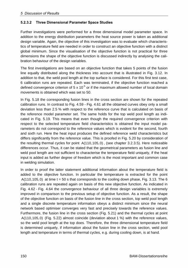
5 Discussion of Results
150 BAM-Dissertationsreihe
5.2.3.2 Three Dimensional Parameter Space Studies
Further investigations were performed for a three dimensional model parameter space. In addition to the energy distribution parameters the heat source power is taken as additional design variable. Again, the objective of this investigation was to evaluate which characteris-tics of temperature field are needed in order to construct an objective function with a distinct global minimum. Since the visualisation of the objective function is not practical for three dimensions the shape of the objective function is discussed indirectly by analysing the cali-bration behaviour of the design variables.
The first investigations are based on an objective function that takes 5 points of the fusion line equally distributed along the thickness into account that is illustrated in Fig. 3.12. In addition to that, the weld pool length at the top surface is considered. For this first test case, 6 calibration runs are repeated. Each was terminated, if the objective function reached a defined convergence criterion of 5 x 10⁻⁵ or if the maximum allowed number of local domain movements is obtained which was set to 50.
In Fig. 5.18 the corresponding fusion lines in the cross section are shown for the repeated calibration runs. In contrast to Fig. 4.59 - Fig. 4.61 all the obtained curves obey only a small deviation less than 2.5 % with respect to the reference curve that is calculated on basis of the reference model parameter set. The same holds for the top weld pool length as indi-cated in Fig. 5.19. This means that even though the required convergence criterion with respect to the selected temperature field characteristics is obtained the input model pa-rameters do not correspond to the reference values which is evident for the second, fourth and sixth run. Here the heat input produces the defined reference weld characteristics but differs significantly from the reference value. This is proofed in Fig. 5.20 by consideration of the resulting thermal cycles for point A(110,105,0) , (see chapter 3.2.3.5). Here noticeable differences occur. Thus, it can be stated that the geometrical parameters as fusion line and weld pool length are not sufficient to characterise the temperature field uniquely, if the heat input is added as further degree of freedom which is the most important and common case in welding simulation.
In order to proof the latter statement additional information about the temperature field is added to the objective function. In particular the temperature is extracted for the point A(110,105,0) at time t = 50 s that corresponds to the cooling down phase, Fig. 3.13. The 6 calibration runs are repeated again on basis of this new objective function. As indicated in Fig. 4.62 - Fig. 4.64 the convergence behaviour of all three design variables is extremely improved in comparison to the previous setup of objective function. As a result, the shape of the objective function on basis of the fusion line in the cross section, top weld pool length and a single discrete temperature information obeys a distinct minimum since the neural network based optimiser converges very fast and precisely towards the reference values. Furthermore, the fusion line in the cross section (Fig. 5.21) and the thermal cycles at point A(110,105,0) (Fig. 5.22) almost coincide (deviation about 1 %) with the reference values, so the weld pool length at the top does. Therefore, the three dimensional temperature field is determined uniquely, if information about the fusion line in the cross section, weld pool length and temperature in terms of thermal cycles, e.g. during cooling down, is at hand.
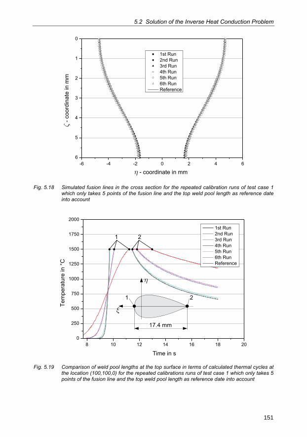
5.2 Solution of the Inverse Heat Conduction Problem
151
-6 -4 -2 0 2 4 66
5
4
3
2
1
0
1st Run2nd Run3rd Run4th Run5th Run6th RunReference
� - coordinate in mm
�- c
oord
inat
e in
mm
Fig. 5.18 Simulated fusion lines in the cross section for the repeated calibration runs of test case 1 which only takes 5 points of the fusion line and the top weld pool length as reference date into account
8 10 12 14 16 18 200
250
500
750
1000
1250
1500
1750
2000
Tem
pera
ture
in°C
Time in s
1st Run2nd Run3rd Run4th Run5th Run6th RunReference
�
�
17.4 mm
1 2
1 2
Fig. 5.19 Comparison of weld pool lengths at the top surface in terms of calculated thermal cycles at the location (100,100,0) for the repeated calibrations runs of test case 1 which only takes 5 points of the fusion line and the top weld pool length as reference date into account
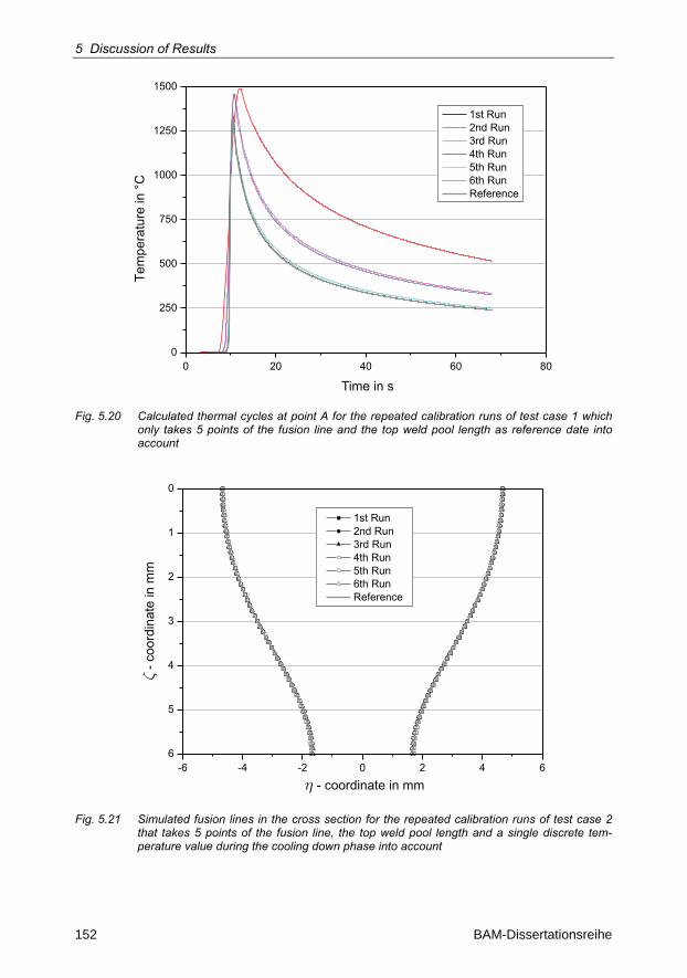
5 Discussion of Results
152 BAM-Dissertationsreihe
0 20 40 60 800
250
500
750
1000
1250
1500
Tem
pera
ture
in°C
Time in s
1st Run2nd Run3rd Run4th Run5th Run6th RunReference
Fig. 5.20 Calculated thermal cycles at point A for the repeated calibration runs of test case 1 which only takes 5 points of the fusion line and the top weld pool length as reference date into account
� - coordinate in mm
�- c
oord
inat
e in
mm
-6 -4 -2 0 2 4 66
5
4
3
2
1
0
1st Run2nd Run3rd Run4th Run5th Run6th RunReference
Fig. 5.21 Simulated fusion lines in the cross section for the repeated calibration runs of test case 2 that takes 5 points of the fusion line, the top weld pool length and a single discrete tem-perature value during the cooling down phase into account
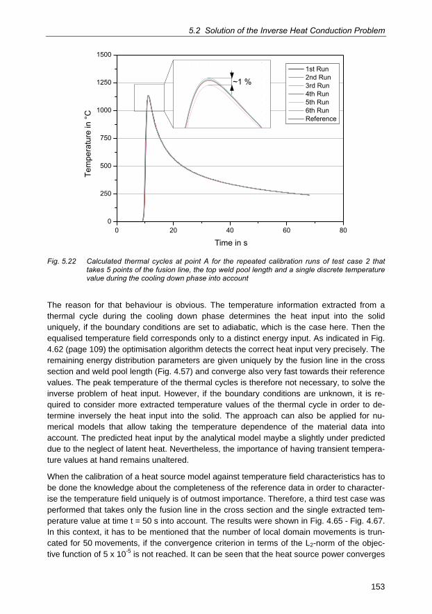
5.2 Solution of the Inverse Heat Conduction Problem
153
0 20 40 60 800
250
500
750
1000
1250
1500
Tem
pera
ture
in°C
Time in s
1st Run2nd Run3rd Run4th Run5th Run6th RunReference
~1 %
Fig. 5.22 Calculated thermal cycles at point A for the repeated calibration runs of test case 2 that takes 5 points of the fusion line, the top weld pool length and a single discrete temperature value during the cooling down phase into account
The reason for that behaviour is obvious. The temperature information extracted from a thermal cycle during the cooling down phase determines the heat input into the solid uniquely, if the boundary conditions are set to adiabatic, which is the case here. Then the equalised temperature field corresponds only to a distinct energy input. As indicated in Fig. 4.62 (page 109) the optimisation algorithm detects the correct heat input very precisely. The remaining energy distribution parameters are given uniquely by the fusion line in the cross section and weld pool length (Fig. 4.57) and converge also very fast towards their reference values. The peak temperature of the thermal cycles is therefore not necessary, to solve the inverse problem of heat input. However, if the boundary conditions are unknown, it is re-quired to consider more extracted temperature values of the thermal cycle in order to de-termine inversely the heat input into the solid. The approach can also be applied for nu-merical models that allow taking the temperature dependence of the material data into account. The predicted heat input by the analytical model maybe a slightly under predicted due to the neglect of latent heat. Nevertheless, the importance of having transient tempera-ture values at hand remains unaltered.
When the calibration of a heat source model against temperature field characteristics has to be done the knowledge about the completeness of the reference data in order to character-ise the temperature field uniquely is of outmost importance. Therefore, a third test case was performed that takes only the fusion line in the cross section and the single extracted tem-perature value at time t = 50 s into account. The results were shown in Fig. 4.65 - Fig. 4.67. In this context, it has to be mentioned that the number of local domain movements is trun-cated for 50 movements, if the convergence criterion in terms of the L2-norm of the objec-tive function of 5 x 10⁻⁵ is not reached. It can be seen that the heat source power converges
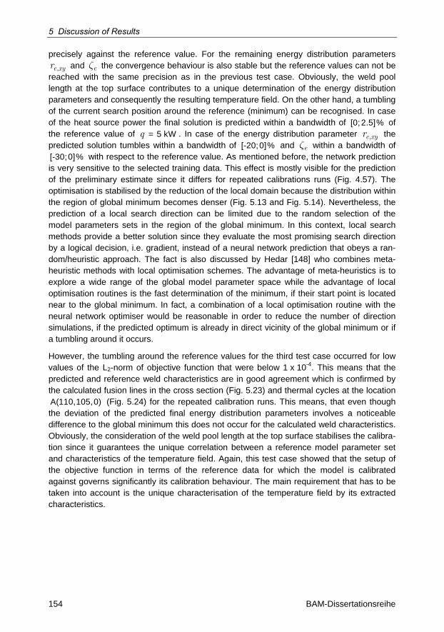
5 Discussion of Results
154 BAM-Dissertationsreihe
precisely against the reference value. For the remaining energy distribution parameters
e xyr , and ez the convergence behaviour is also stable but the reference values can not be reached with the same precision as in the previous test case. Obviously, the weld pool length at the top surface contributes to a unique determination of the energy distribution parameters and consequently the resulting temperature field. On the other hand, a tumbling of the current search position around the reference (minimum) can be recognised. In case of the heat source power the final solution is predicted within a bandwidth of [0;2.5]% of the reference value of q = 5 kW . In case of the energy distribution parameter e xyr , the predicted solution tumbles within a bandwidth of [-20;0]% and ez within a bandwidth of [-30;0]% with respect to the reference value. As mentioned before, the network prediction is very sensitive to the selected training data. This effect is mostly visible for the prediction of the preliminary estimate since it differs for repeated calibrations runs (Fig. 4.57). The optimisation is stabilised by the reduction of the local domain because the distribution within the region of global minimum becomes denser (Fig. 5.13 and Fig. 5.14). Nevertheless, the prediction of a local search direction can be limited due to the random selection of the model parameters sets in the region of the global minimum. In this context, local search methods provide a better solution since they evaluate the most promising search direction by a logical decision, i.e. gradient, instead of a neural network prediction that obeys a ran-dom/heuristic approach. The fact is also discussed by Hedar [148] who combines meta-heuristic methods with local optimisation schemes. The advantage of meta-heuristics is to explore a wide range of the global model parameter space while the advantage of local optimisation routines is the fast determination of the minimum, if their start point is located near to the global minimum. In fact, a combination of a local optimisation routine with the neural network optimiser would be reasonable in order to reduce the number of direction simulations, if the predicted optimum is already in direct vicinity of the global minimum or if a tumbling around it occurs.
However, the tumbling around the reference values for the third test case occurred for low values of the L2-norm of objective function that were below 1 x 10⁻⁴. This means that the predicted and reference weld characteristics are in good agreement which is confirmed by the calculated fusion lines in the cross section (Fig. 5.23) and thermal cycles at the location A(110,105,0) (Fig. 5.24) for the repeated calibration runs. This means, that even though the deviation of the predicted final energy distribution parameters involves a noticeable difference to the global minimum this does not occur for the calculated weld characteristics. Obviously, the consideration of the weld pool length at the top surface stabilises the calibra-tion since it guarantees the unique correlation between a reference model parameter set and characteristics of the temperature field. Again, this test case showed that the setup of the objective function in terms of the reference data for which the model is calibrated against governs significantly its calibration behaviour. The main requirement that has to be taken into account is the unique characterisation of the temperature field by its extracted characteristics.
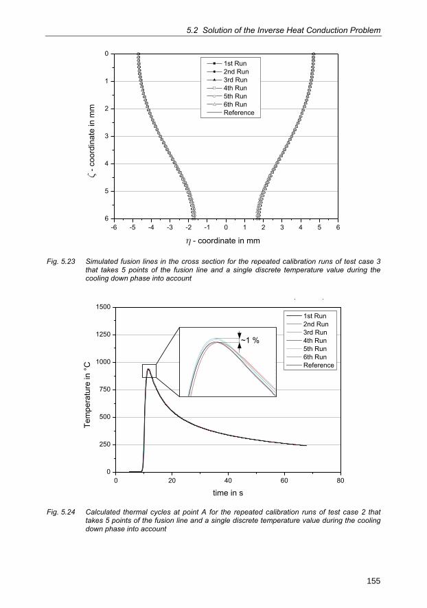
5.2 Solution of the Inverse Heat Conduction Problem
155
-6 -5 -4 -3 -2 -1 0 1 2 3 4 5 66
5
4
3
2
1
01st Run2nd Run3rd Run4th Run5th Run6th RunReference
� - coordinate in mm
�- c
oord
inat
e in
mm
Fig. 5.23 Simulated fusion lines in the cross section for the repeated calibration runs of test case 3 that takes 5 points of the fusion line and a single discrete temperature value during the cooling down phase into account
0 20 40 60 800
250
500
750
1000
1250
1500
Tem
pera
ture
in°C
time in s
1st Run2nd Run3rd Run4th Run5th Run6th RunReference
~1 %
Fig. 5.24 Calculated thermal cycles at point A for the repeated calibration runs of test case 2 that takes 5 points of the fusion line and a single discrete temperature value during the cooling down phase into account
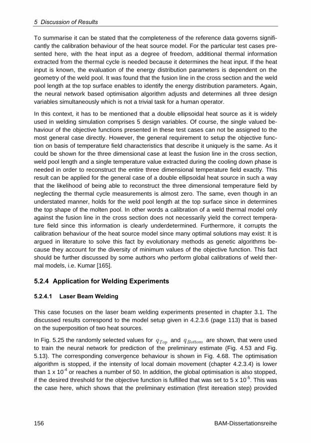
5 Discussion of Results
156 BAM-Dissertationsreihe
To summarise it can be stated that the completeness of the reference data governs signifi-cantly the calibration behaviour of the heat source model. For the particular test cases pre-sented here, with the heat input as a degree of freedom, additional thermal information extracted from the thermal cycle is needed because it determines the heat input. If the heat input is known, the evaluation of the energy distribution parameters is dependent on the geometry of the weld pool. It was found that the fusion line in the cross section and the weld pool length at the top surface enables to identify the energy distribution parameters. Again, the neural network based optimisation algorithm adjusts and determines all three design variables simultaneously which is not a trivial task for a human operator.
In this context, it has to be mentioned that a double ellipsoidal heat source as it is widely used in welding simulation comprises 5 design variables. Of course, the single valued be-haviour of the objective functions presented in these test cases can not be assigned to the most general case directly. However, the general requirement to setup the objective func-tion on basis of temperature field characteristics that describe it uniquely is the same. As it could be shown for the three dimensional case at least the fusion line in the cross section, weld pool length and a single temperature value extracted during the cooling down phase is needed in order to reconstruct the entire three dimensional temperature field exactly. This result can be applied for the general case of a double ellipsoidal heat source in such a way that the likelihood of being able to reconstruct the three dimensional temperature field by neglecting the thermal cycle measurements is almost zero. The same, even though in an understated manner, holds for the weld pool length at the top surface since in determines the top shape of the molten pool. In other words a calibration of a weld thermal model only against the fusion line in the cross section does not necessarily yield the correct tempera-ture field since this information is clearly underdetermined. Furthermore, it corrupts the calibration behaviour of the heat source model since many optimal solutions may exist: It is argued in literature to solve this fact by evolutionary methods as genetic algorithms be-cause they account for the diversity of minimum values of the objective function. This fact should be further discussed by some authors who perform global calibrations of weld ther-mal models, i.e. Kumar [165].
5.2.4 Application for Welding Experiments
5.2.4.1 Laser Beam Welding
This case focuses on the laser beam welding experiments presented in chapter 3.1. The discussed results correspond to the model setup given in 4.2.3.6 (page 113) that is based on the superposition of two heat sources.
In Fig. 5.25 the randomly selected values for Topq and Bottomq are shown, that were used to train the neural network for prediction of the preliminary estimate (Fig. 4.53 and Fig. 5.13). The corresponding convergence behaviour is shown in Fig. 4.68. The optimisation algorithm is stopped, if the intensity of local domain movement (chapter 4.2.3.4) is lower than 1 x 10⁻⁴ or reaches a number of 50. In addition, the global optimisation is also stopped, if the desired threshold for the objective function is fulfilled that was set to 5 x 10⁻⁵. This was the case here, which shows that the preliminary estimation (first itereation step) provided
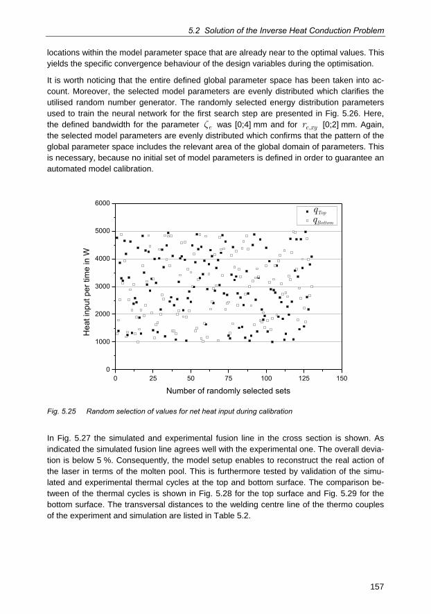
5.2 Solution of the Inverse Heat Conduction Problem
157
locations within the model parameter space that are already near to the optimal values. This yields the specific convergence behaviour of the design variables during the optimisation.
It is worth noticing that the entire defined global parameter space has been taken into ac-count. Moreover, the selected model parameters are evenly distributed which clarifies the utilised random number generator. The randomly selected energy distribution parameters used to train the neural network for the first search step are presented in Fig. 5.26. Here, the defined bandwidth for the parameter ez was [0;4] mm and for e xyr , [0;2] mm. Again, the selected model parameters are evenly distributed which confirms that the pattern of the global parameter space includes the relevant area of the global domain of parameters. This is necessary, because no initial set of model parameters is defined in order to guarantee an automated model calibration.
0 25 50 75 100 125 1500
1000
2000
3000
4000
5000
6000
Hea
tinp
utpe
rtim
ein
W
Number of randomly selected sets
qTop
qBottom
Fig. 5.25 Random selection of values for net heat input during calibration
In Fig. 5.27 the simulated and experimental fusion line in the cross section is shown. As indicated the simulated fusion line agrees well with the experimental one. The overall devia-tion is below 5 %. Consequently, the model setup enables to reconstruct the real action of the laser in terms of the molten pool. This is furthermore tested by validation of the simu-lated and experimental thermal cycles at the top and bottom surface. The comparison be-tween of the thermal cycles is shown in Fig. 5.28 for the top surface and Fig. 5.29 for the bottom surface. The transversal distances to the welding centre line of the thermo couples of the experiment and simulation are listed in Table 5.2.
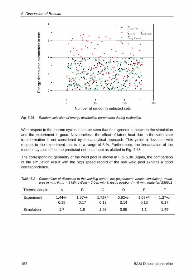
5 Discussion of Results
158 BAM-Dissertationsreihe
0 50 100 150
0
1
2
3
4
Number of randomly selected sets
� �e,Top e,Bottom=re,xy,Top
re,xy,BottomE
nerg
y di
strib
utio
n pa
ram
eter
s in
mm
Fig. 5.26 Random selection of energy distribution parameters during calibration
With respect to the thermo cycles it can be seen that the agreement between the simulation and the experiment is good. Nevertheless, the effect of latent heat due to the solid-state transformation is not considered by the analytical approach. This yields a deviation with respect to the experiment that is in a range of 5 %. Furthermore, the linearisation of the model may also effect the predicted net heat input as plotted in Fig. 4.68.
The corresponding geometry of the weld pool is shown in Fig. 5.30. Again, the comparison of the simulation result with the high speed record of the real weld pool exhibits a good correspondence.
Table 5.2 Comparison of distances to the welding centre line (experiment versus simulation); meas-ures in mm, PLaser = 8 kW, vWeld = 3.0 m min-1, focus position f = -6 mm, material: S355J2
Thermo couple A B C D E F
Experiment 1.44+/-0.15
1.57+/-0.17
1.72+/-0.13
0.92+/-0.14
1.08+/-0.13
1.37+/-0.17
Simulation 1.7 1.8 1.95 0.95 1.1 1.49
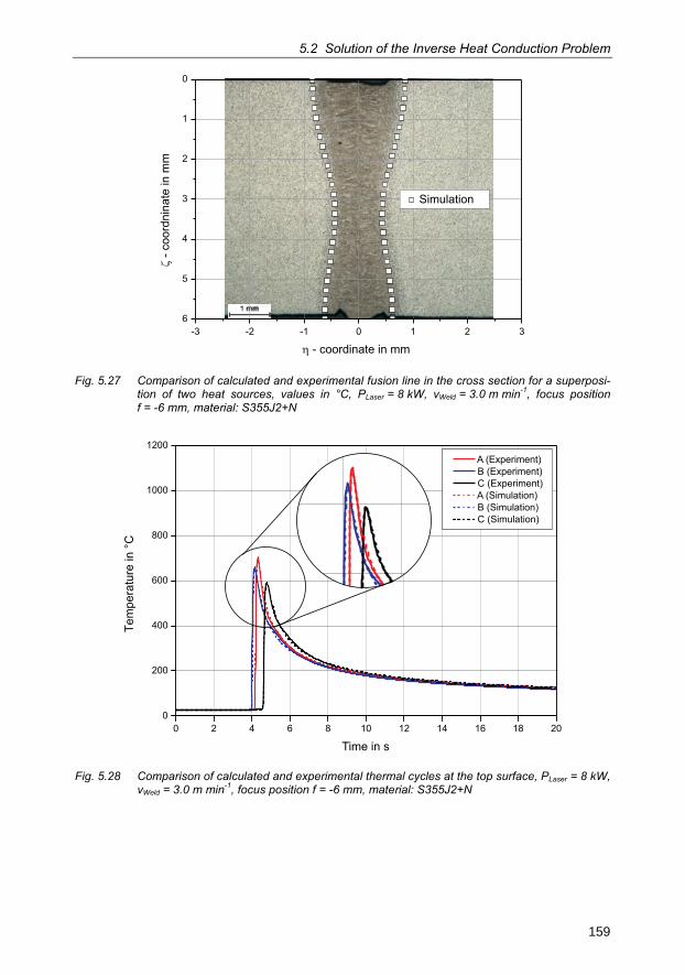
5.2 Solution of the Inverse Heat Conduction Problem
159
-3 -2 -1 0 1 2 36
5
4
3
2
1
0
�- c
oord
nina
te in
mm
� - coordinate in mm
Simulation
Fig. 5.27 Comparison of calculated and experimental fusion line in the cross section for a superposi-tion of two heat sources, values in °C, PLaser = 8 kW, vWeld = 3.0 m min-1, focus position f = -6 mm, material: S355J2+N
0 2 4 6 8 10 12 14 16 18 200
200
400
600
800
1000
1200A (Experiment)B (Experiment)C (Experiment)A (Simulation)B (Simulation)C (Simulation)
Tem
pera
ture
in°C
Time in s
Fig. 5.28 Comparison of calculated and experimental thermal cycles at the top surface, PLaser = 8 kW, vWeld = 3.0 m min-1, focus position f = -6 mm, material: S355J2+N
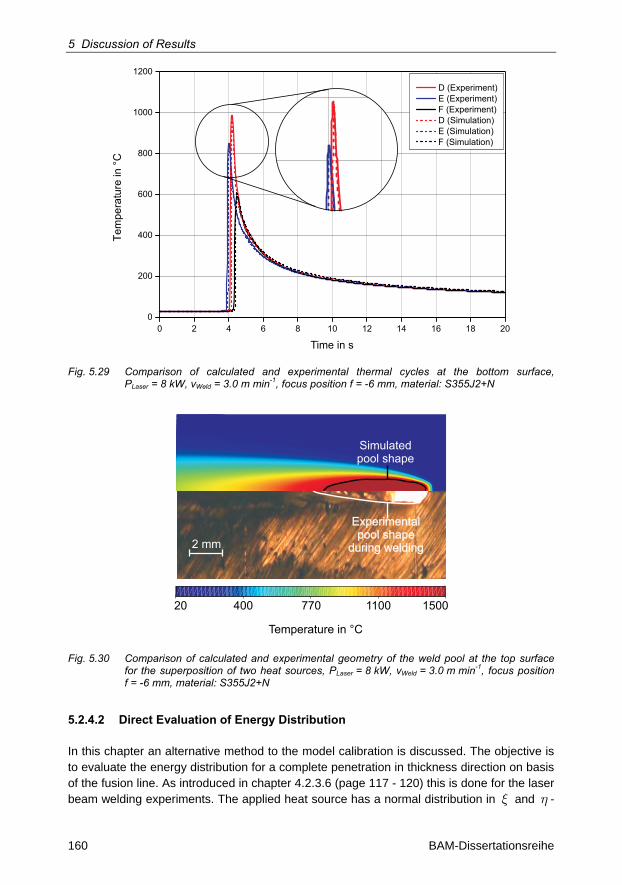
5 Discussion of Results
160 BAM-Dissertationsreihe
0 2 4 6 8 10 12 14 16 18 200
200
400
600
800
1000
1200
D (Experiment)E (Experiment)F (Experiment)D (Simulation)E (Simulation)F (Simulation)
Tem
pera
ture
in°C
Time in s
Fig. 5.29 Comparison of calculated and experimental thermal cycles at the bottom surface, PLaser = 8 kW, vWeld = 3.0 m min-1, focus position f = -6 mm, material: S355J2+N
Experimentalpool shape
during welding
Experimentalpool shape
during welding
Simulatedpool shape
20 400 770 1100 1500
Temperature in °C
2 mm
Fig. 5.30 Comparison of calculated and experimental geometry of the weld pool at the top surface for the superposition of two heat sources, PLaser = 8 kW, vWeld = 3.0 m min-1, focus position f = -6 mm, material: S355J2+N
5.2.4.2 Direct Evaluation of Energy Distribution
In this chapter an alternative method to the model calibration is discussed. The objective is to evaluate the energy distribution for a complete penetration in thickness direction on basis of the fusion line. As introduced in chapter 4.2.3.6 (page 117 - 120) this is done for the laser beam welding experiments. The applied heat source has a normal distribution in x and h -
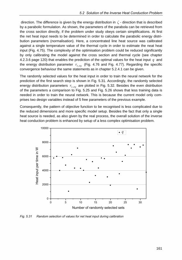
5.2 Solution of the Inverse Heat Conduction Problem
161
direction. The difference is given by the energy distribution in z - direction that is described by a parabolic formulation. As shown, the parameters of the parabola can be retrieved from the cross section directly, if the problem under study obeys certain simplifications. At first the net heat input needs to be determined in order to calculate the parabolic energy distri-bution parameters (normalisation). Here, a concentrated line heat source was calibrated against a single temperature value of the thermal cycle in order to estimate the neat heat input (Fig. 4.75). The complexity of the optimisation problem could be reduced significantly by only calibrating the model against the cross section and thermal cycle (see chapter 4.2.3.6 page 120) that enables the prediction of the optimal values for the heat input q and the energy distribution parameter e xyr , (Fig. 4.76 and Fig. 4.77). Regarding the specific convergence behaviour the same statements as in chapter 5.2.4.1 can be given.
The randomly selected values for the heat input in order to train the neural network for the prediction of the first search step is shown in Fig. 5.31. Accordingly, the randomly selected energy distribution parameters e xyr , are plotted in Fig. 5.32. Besides the even distribution of the parameters a comparison to Fig. 5.25 and Fig. 5.26 shows that less training data is needed in order to train the neural network. This is because the current model only com-prises two design variables instead of 5 free parameters of the previous example.
Consequently, the pattern of objective function to be recognised is less complicated due to the reduced dimensions and more specific model setup. Besides the fact that only a single heat source is needed, as also given by the real process, the overall solution of the inverse heat conduction problem is enhanced by setup of a less complex optimisation problem.
0 5 10 15 20 25 300
2000
4000
6000
8000
10000q
Hea
tinp
utpe
rtim
ein
W
Number of randomly selected sets
Fig. 5.31 Random selection of values for net heat input during calibration
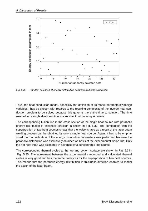
5 Discussion of Results
162 BAM-Dissertationsreihe
0 5 10 15 20 25 300
0.5
1.0
1.5
2.0
Number of randomly selected sets
re,xy
Ene
rgy
dist
ribut
ion
para
met
ers
in m
m
Fig. 5.32 Random selection of energy distribution parameters during calibration
Thus, the heat conduction model, especially the definition of its model parameters(=design variables), has be chosen with regards to the resulting complexity of the inverse heat con-duction problem to be solved because this governs the entire time to solution. The time needed for a single direct solution is a sufficient but not unique criteria.
The corresponding fusion line in the cross section of the single heat source with parabolic energy distribution in thickness direction is shown in Fig. 5.33. The comparison with the superposition of two heat sources shows that the waisty shape as a result of the laser beam welding process can be obtained by only a single heat source. Again, it has to be empha-sised that no calibration of the energy distribution parameters was performed because the parabolic distribution was exclusively obtained on basis of the experimental fusion line. Only the net heat input was estimated in advance by a concentrated line source.
The corresponding thermal cycles at the top and bottom surface are shown in Fig. 5.34 - Fig. 5.35. The agreement between the experimentally recorded and calculated thermal cycles is very good and has the same quality as for the superposition of two heat sources. This means that the parabolic energy distribution in thickness direction enables to model the action of the laser beam.
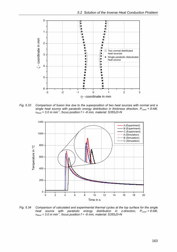
5.2 Solution of the Inverse Heat Conduction Problem
163
-3 -2 -1 0 1 2 36
5
4
3
2
1
0
Two normal distributedheat sourcesSingle parabolic distrubutedheat source
� - coordinate in mm
�- c
oord
inat
e in
mm
Fig. 5.33 Comparison of fusion line due to the superposition of two heat sources with normal and a single heat source with parabolic energy distribution in thickness direction, PLaser = 8 kW, vWeld = 3.0 m min-1, focus position f = -6 mm, material: S355J2+N
0 2 4 6 8 10 12 14 16 18 200
200
400
600
800
1000
1200A (Experiment)B (Experiment)C (Experiment)A (Simulation)B (Simulation)C (Simulation)
Tem
pera
ture
in°C
Time in s
Fig. 5.34 Comparison of calculated and experimental thermal cycles at the top surface for the single heat source with parabolic energy distribution in z-direction, PLaser = 8 kW, vWeld = 3.0 m min-1, focus position f = -6 mm, material: S355J2+N
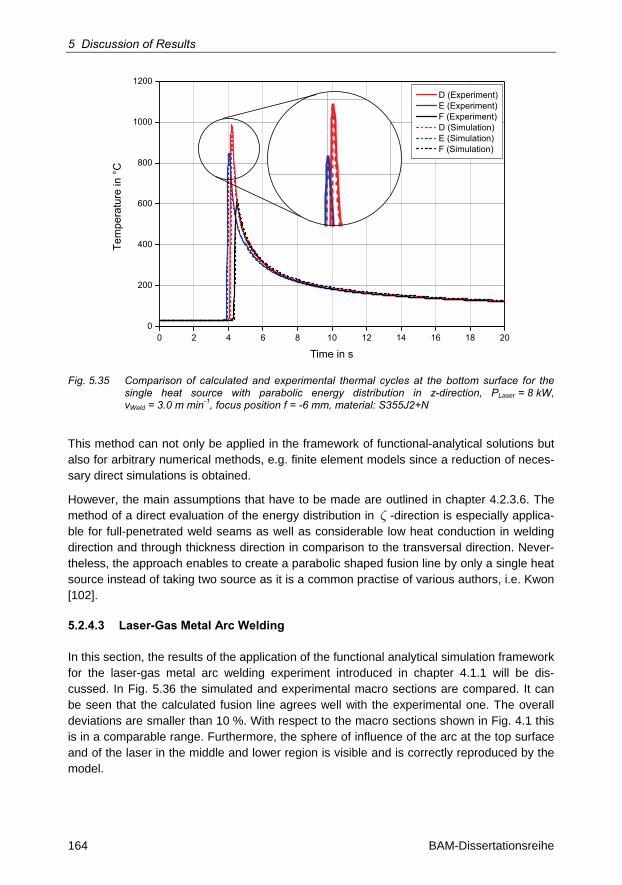
5 Discussion of Results
164 BAM-Dissertationsreihe
0 2 4 6 8 10 12 14 16 18 200
200
400
600
800
1000
1200D (Experiment)E (Experiment)F (Experiment)D (Simulation)E (Simulation)F (Simulation)
Tem
pera
ture
in°C
Time in s
Fig. 5.35 Comparison of calculated and experimental thermal cycles at the bottom surface for the single heat source with parabolic energy distribution in z-direction, PLaser = 8 kW, vWeld = 3.0 m min-1, focus position f = -6 mm, material: S355J2+N
This method can not only be applied in the framework of functional-analytical solutions but also for arbitrary numerical methods, e.g. finite element models since a reduction of neces-sary direct simulations is obtained.
However, the main assumptions that have to be made are outlined in chapter 4.2.3.6. The method of a direct evaluation of the energy distribution in z -direction is especially applica-ble for full-penetrated weld seams as well as considerable low heat conduction in welding direction and through thickness direction in comparison to the transversal direction. Never-theless, the approach enables to create a parabolic shaped fusion line by only a single heat source instead of taking two source as it is a common practise of various authors, i.e. Kwon [102].
5.2.4.3 Laser-Gas Metal Arc Welding
In this section, the results of the application of the functional analytical simulation framework for the laser-gas metal arc welding experiment introduced in chapter 4.1.1 will be dis-cussed. In Fig. 5.36 the simulated and experimental macro sections are compared. It can be seen that the calculated fusion line agrees well with the experimental one. The overall deviations are smaller than 10 %. With respect to the macro sections shown in Fig. 4.1 this is in a comparable range. Furthermore, the sphere of influence of the arc at the top surface and of the laser in the middle and lower region is visible and is correctly reproduced by the model.
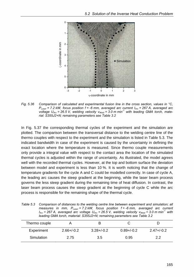
5.2 Solution of the Inverse Heat Conduction Problem
165
-3 -2 -1 0 1 2 36
5
4
3
2
1
0
�-coordinate in mm
Simulation -c
oord
inat
e in
mm
Fig. 5.36 Comparison of calculated and experimental fusion line in the cross section, values in °C, PLaser = 7.2 kW, focus position f = -6 mm, averaged arc current IArc = 267 A, averaged arc voltage UArc = 26.5 V, welding velocity vWeld = 3.0 m min-1 with leading GMA torch, mate-rial: S355J2+N; remaining parameters see Table 3.2
In Fig. 5.37 the corresponding thermal cycles of the experiment and the simulation are plotted. The comparison between the transversal distance to the welding centre line of the thermo couples with respect to the experiment and the simulation is listed in Table 5.3. The indicated bandwidth in case of the experiment is caused by the uncertainty in defining the exact location where the temperature is measured. Since thermo couple measurements only provide a integral value with respect to the contact area the location of the simulated thermal cycles is adjusted within the range of uncertainty. As illustrated, the model agrees well with the recorded thermal cycles. However, at the top and bottom surface the deviation between model and experiment is less than 10 %. It is worth noticing that the change of temperature gradients for the cycle A and C could be modelled correctly. In case of cycle A, the leading arc causes the steep gradient at the beginning, while the laser beam process governs the less steep gradient during the remaining time of heat diffusion. In contrast, the laser beam process causes the steep gradient at the beginning of cycle C while the arc process is responsible for the remaining shape of the thermal cycle.
Table 5.3 Comparison of distances to the welding centre line between experiment and simulation; all measures in mm, PLaser = 7.2 kW, focus position f = -6 mm, averaged arc current IArc = 267 A, averaged arc voltage UArc = 26.5 V, welding velocity vWeld = 3.0 m min-1 with leading GMA torch, material: S355J2+N; remaining parameters see Table 3.2
Thermo couple A B C D
Experiment 2.66+/-0.2 3.28+/-0.2 0.89+/-0.2 2.47+/-0.2
Simulation 2.75 3.5 0.95 2.2
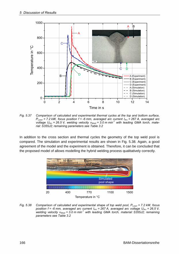
5 Discussion of Results
166 BAM-Dissertationsreihe
0 2 4 6 8 10 12 14
Time in s
A (Experiment)B (Experiment)C (Experiment)D (Experiment)A (Simulation)B (Simulation)C (Simulation)D (Simulation)
D
BA
C
0
200
400
600
800
1000
Tem
pera
ture
in °
CA
C
B D
Fig. 5.37 Comparison of calculated and experimental thermal cycles at the top and bottom surface, PLaser = 7.2 kW, focus position f = -6 mm, averaged arc current IArc = 267 A, averaged arc voltage UArc = 26.5 V, welding velocity vWeld = 3.0 m min-1 with leading GMA torch, mate-rial: S355J2; remaining parameters see Table 3.2
In addition to the cross section and thermal cycles the geometry of the top weld pool is compared. The simulation and experimental results are shown in Fig. 5.38. Again, a good agreement of the model and the experiment is obtained. Therefore, it can be concluded that the proposed model of allows modelling the hybrid welding process qualitatively correctly.
Experimentalend crater
20 400 770 1100 1500Temperature in °C
10 mm
Simulatedpool shape
Fig. 5.38 Comparison of calculated and experimental shape of top weld pool, PLaser = 7.2 kW, focus position f = -6 mm, averaged arc current IArc = 267 A, averaged arc voltage UArc = 26.5 V, welding velocity vWeld = 3.0 m min-1 with leading GMA torch, material: S355J2; remaining parameters see Table 3.2

5.2 Solution of the Inverse Heat Conduction Problem
167
With respect to the evaluation of the heat input for the top and bottom heat source as pre-sented in chapter 4.2.3.6, Fig. 4.81 it has to be mentioned, that the linearisation of the heat conduction model influences the predicted value for the net heat input. Especially, the ne-glect of latent heat may have an effect on the reconstructed heat input [114]. Furthermore, for thin sheets the specific boundary conditions have to be considered.
Nevertheless, the calculated temperature field resembles the experimental one sufficiently. The needed reduction of the heat conductivity corresponds to a temperature range near the solidification temperature. Thus, taking the thermo physical material date near to the solidi-fication temperature yields a good prediction of the weld pool and thermal cycles in the high temperature range. This set of model parameters can then be used as start values in a non-linear finite element model analysis.
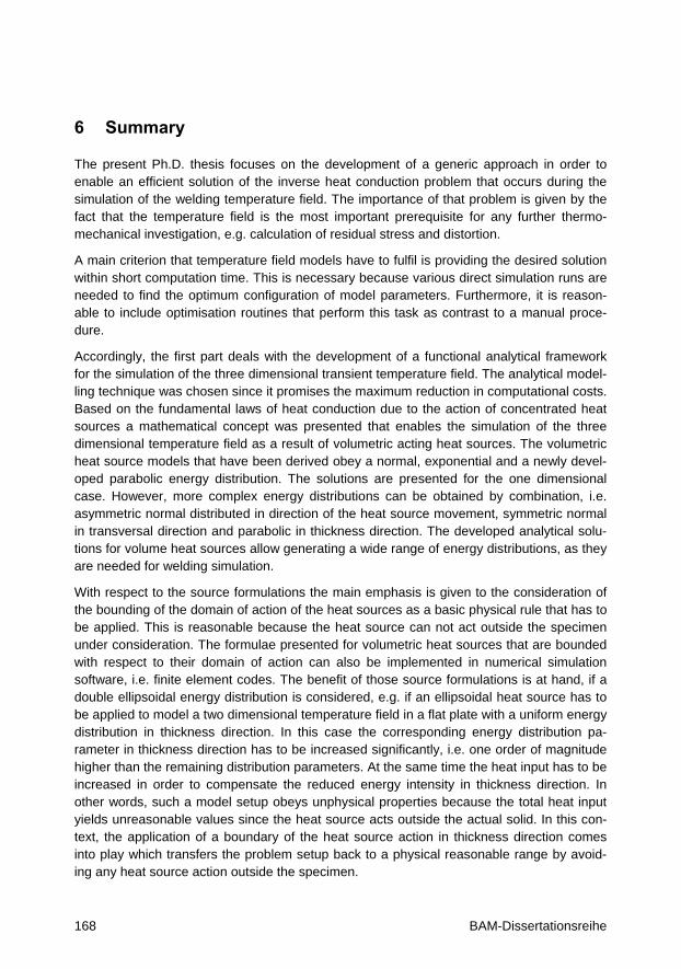
168 BAM-Dissertationsreihe
6 Summary
The present Ph.D. thesis focuses on the development of a generic approach in order to enable an efficient solution of the inverse heat conduction problem that occurs during the simulation of the welding temperature field. The importance of that problem is given by the fact that the temperature field is the most important prerequisite for any further thermo-mechanical investigation, e.g. calculation of residual stress and distortion.
A main criterion that temperature field models have to fulfil is providing the desired solution within short computation time. This is necessary because various direct simulation runs are needed to find the optimum configuration of model parameters. Furthermore, it is reason-able to include optimisation routines that perform this task as contrast to a manual proce-dure.
Accordingly, the first part deals with the development of a functional analytical framework for the simulation of the three dimensional transient temperature field. The analytical model-ling technique was chosen since it promises the maximum reduction in computational costs. Based on the fundamental laws of heat conduction due to the action of concentrated heat sources a mathematical concept was presented that enables the simulation of the three dimensional temperature field as a result of volumetric acting heat sources. The volumetric heat source models that have been derived obey a normal, exponential and a newly devel-oped parabolic energy distribution. The solutions are presented for the one dimensional case. However, more complex energy distributions can be obtained by combination, i.e. asymmetric normal distributed in direction of the heat source movement, symmetric normal in transversal direction and parabolic in thickness direction. The developed analytical solu-tions for volume heat sources allow generating a wide range of energy distributions, as they are needed for welding simulation.
With respect to the source formulations the main emphasis is given to the consideration of the bounding of the domain of action of the heat sources as a basic physical rule that has to be applied. This is reasonable because the heat source can not act outside the specimen under consideration. The formulae presented for volumetric heat sources that are bounded with respect to their domain of action can also be implemented in numerical simulation software, i.e. finite element codes. The benefit of those source formulations is at hand, if a double ellipsoidal energy distribution is considered, e.g. if an ellipsoidal heat source has to be applied to model a two dimensional temperature field in a flat plate with a uniform energy distribution in thickness direction. In this case the corresponding energy distribution pa-rameter in thickness direction has to be increased significantly, i.e. one order of magnitude higher than the remaining distribution parameters. At the same time the heat input has to be increased in order to compensate the reduced energy intensity in thickness direction. In other words, such a model setup obeys unphysical properties because the total heat input yields unreasonable values since the heat source acts outside the actual solid. In this con-text, the application of a boundary of the heat source action in thickness direction comes into play which transfers the problem setup back to a physical reasonable range by avoid-ing any heat source action outside the specimen.
6 Summary
169
The final functional-analytical expressions that are presented refer to the integrand function which is equivalent to the temperature response due to instantaneous heat sources. The continuous action and corresponding temperature field can be obtained by means of a numerical integration. The resulting temperature field is transient. Here, the effect of a stop of heat source action is of interest. The classical method on basis of additional negative valued heat sources that is still applied by many authors was compared with an alternative approach that only takes a single heat source into account. Moreover, the usage of only a single heat source by adjusting the integration limits enables to reduce the computational time significantly. Consequently, this approach should be preferred, if the stop of heat source is to be modelled. This is the case, if the cooling down phase has to be taken into account but also if the heat source changes its direction of movement. The basis for the analytical modelling of heat sources that are moving on arbitrary curved trajectories has already been reported in literature. The fundamental assumption is that the welding trajec-tory is discretised into linear sub-paths that are arbitrary oriented with regards to the global coordinate system that is aligned to the specimen. This technique is also applied here. The movement of the heat source on a linear sub-path that has a certain orientation to the global coordinate system can be implemented by usage of the global velocity vector whose components are given by the direction cosine. It was found that this known approach works well for concentrated heat sources as it is published Cao [123]. Furthermore, it can only be applied for heat sources that have a symmetric distribution in the plane of their movement, i.e. circular GAUSSIAN distribution at the top surface and normal distributed in thickness direction. However, it was proven that this approach cannot be applied for asymmetrically distributed heat sources like i.e. double ellipsoidal heat sources. This is because the energy distribution parameters are expressed in terms of the local coordinate system of the heat source. Thus, a coordinate transformation was implemented that maps the local tempera-ture field into the global domain by translation and rotation. It is therefore possible to calcu-late the global temperature field for asymmetrically distributed volume heat sources that move on sub-paths that have an arbitrary orientation with respect to the global reference frame. Together with the consideration of a finite geometry this is an extension to the ap-proaches that can be found in literature, i.e. Winczek [124].
It was discussed that the modelling of the movement on curved trajectories requires the decomposition of the welding trajectory into linear sub-paths, each with a certain orientation to the global coordinate system. Furthermore, dummy heat sources have to be introduced in order to consider the change of the direction of movement. This means that the more complex the welding trajectory is defined the more the computational efforts increase. In this context alternative methods of modelling the action of volumetric heat sources on finite thick geometries were investigated. In particular, the well known method of image sources was compared with the series expansion after FOURIER. It was found that for small FOURIER numbers, the method of images obeys computational benefits. In other words, if the tem-perature gradient between the top and bottom surface is high then the convergence of the series of image sources is faster than the FOURIER series. In contrast to that the FOURIER series converges significantly faster than the method of images, if the FOURIER number is high. This is the case for low temperature gradients between top and bottom surface, i.e. during the cooling down phase. Furthermore, the FOURIER series expansion for normal distributed heat sources has been presented which is based on the complex error function and has not been given in literature before.
6 Summary
170 BAM-Dissertationsreihe
The movement of a double ellipsoidal heat source on curved trajectories acting on a geo-metrically finite specimen was validated with a finite element model because no analytical reference exists in literature. In case of a linear finite element model with temperature inde-pendent thermo physical properties the correspondence between the analytical and finite element approach is excellent. The most significant advantage of analytical approaches can be emphasised, if the calculation of thermo cycles or the fusion line in the cross section is of interest. The evaluation of the thermal cycles as well as the fusion line in the cross section is completely dedicated to the post processing, if a finite element model has been employed because the entire system of equations has to be solved before. The situation is different, if analytical models are applied. Here the temperature at any point and any time can be cal-culated independently on neighbouring points. This is a great advantage especially if the calibration data is created that mainly is based on the fusion line in the cross section and thermal cycles. This is the fundamental criterion to enable an efficient solution of the inverse heat conduction problem.
In addition to the development of functional analytical models for calculation of a three di-mensional transient temperature field an important part of the thesis was dedicated to the global calibration of volume heat source models. The basis for the successful calibration of weld thermal models against experimental reference data is the prerequisite of having knowledge about the sensitivity with regards to certain weld characteristics. Exemplarily for a normal distributed heat source the sensitivity with respect to the top and bottom weld pool width, weld pool length and depth of penetration was plotted for a two dimensional parame-ter space. In order to account for the high gradients of the weld characteristics a matrix of 160 x 160 elements was considered. Again, the low computational costs of analytical mod-els allow performing these investigations which is not possible in case of a finite element model. It was found, that the gradient of the weld characteristics is very low in some regions while in other regions it is very high. This change of behaviour has to be known and consid-ered during calibration.
The calibration of the model is based on the minimisation of an objective function. A further part of investigations focussed on the evaluation of the shape of the objective function in dependence of the considered reference data. Several scenarios were studied here. In case of a two dimensional parameter space and a fixed heat input the optimisation problem is uniquely determined, if the fusion line in the cross section is taken as reference data. On the other hand, if only the top weld pool width is the reference a multi valued problem has been constructed.
The global optimisation was performed by application of a neural network based optimisa-tion algorithm. For the two dimensional objective function its main behaviour could be illus-trated. This is the combination of a global and local search methodology. The advantage against a pure local optimisation algorithm is that no initial value has to be defined. A further strength of the employed algorithm is that the global pattern of the objective function is recognised by a random distribution of only a few points within the global domain of pa-rameters. The regions of minimum values of the objective function can be found efficiently by this method. However, it was presented that the efficiency of the global optimisation algorithm depends not only on its setup but also strongly on its underlying objective func-tion. In case of two design variables the reference data has to contain information about the fusion line in the cross section and weld pool length at the top surface. For this case the
6 Summary
171
optimiser finds the global minimum by only a few iterations because it is well accentuated. On the other hand, if only the weld pool width at the top surface is taken into account a curved region of very low values of the objective function exists. The optimiser is trapped within these regions because the gradient towards the global minimum is very low. The underlying problem statement is multi valued.
The test case of investigations of the influence of the shape of the objective function on the global calibration or optimisation behaviour respectively, was extended to a three dimen-sional parameter space by taking the heat input as additional degree of freedom. It could be demonstrated that the global minimum can be found by a few iterations, if the objective function was setup on basis of the fusion line in the cross section, weld pool length at the top surface and a single temperature value extracted during the cooling down phase. In other words this means that the objective function is single valued. If only the fusion line in the cross section and the weld pool length at the top surface are taken as reference data then the problem is multi valued because the geometry of the weld pool can be reproduced by various energy distributions and heat input. The single temperature during the cooling down phase enables to recalculate the corresponding energy input. If this is known, the geometrical information about the molten zone in terms of the fusion line in the cross sec-tion and the weld pool at the top surface yields a single valued problem. This result has to be seen in comparison to the usage of evolutionary methods that account for the diversity of the objective function [165].
To summarise it can be stated that the efficient solution of the inverse heat conduction problem requires fast solutions to the temperature field on the one hand but on the other hand the knowledge about the shape of the objective function in dependence on the refer-ence data is of outmost importance. The three dimensional parameter space studies showed that the best calibration results can be obtained, if the fusion line in the cross sec-tion, weld pool length at the top surface and transient temperature information is at hand. Consequently, if the heat input is unknown a calibration only against the fusion line does not necessarily provide the global minimum. This main conclusion obtained from the three dimensional model parameter space can directly be transferred onto the five dimensional parameter space of a double ellipsoidal heat source. Therefore, the uniqueness of the tem-perature field has to be ensured in dependence on the considered reference data and de-sign variables.
In addition to the studies performed above a method was developed to reduce the dimen-sion of the optimisation problem. For this purpose, the derivation of the energy distribution in thickness direction for a laser beam welding experiment has been applied. The applica-tion of the newly introduced parabolic energy distribution allowed defining a relationship between the geometry of the fusion line in the cross section and the corresponding para-bolic energy distribution in thickness direction. The approach enables to model the laser beam welding experiment only by means of a single heat source and with a reduced num-ber of design variables which enhances the inverse problem solution significantly, Again, it has to be regarded that this method can also be used for numerical simulation models.
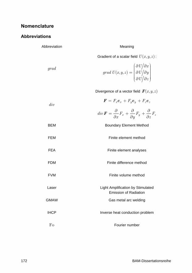
172 BAM-Dissertationsreihe
Nomenclature
Abbreviations
Abbreviation Meaning
grad
Gradient of a scalar field U x y z( , , ) :
U x
grad U x y z U y
U z
( , , )
æ ö¶ ¶ ÷ç ÷ç ÷ç ÷= ¶ ¶ç ÷ç ÷ç ÷÷ç ÷ç¶ ¶è ø
div
Divergence of a vector field x y z( , , )F
x x y y z zF F F= + +F e e e
x y zdiv F F Fx y z
¶ ¶ ¶= + +
¶ ¶ ¶F
BEM Boundary Element Method
FEM Finite element method
FEA Finite element analyses
FDM Finite difference method
FVM Finite volume method
Laser Light Amplification by Stimulated Emission of Radiation
GMAW Gas metal arc welding
IHCP Inverse heat conduction problem
Fo Fourier number
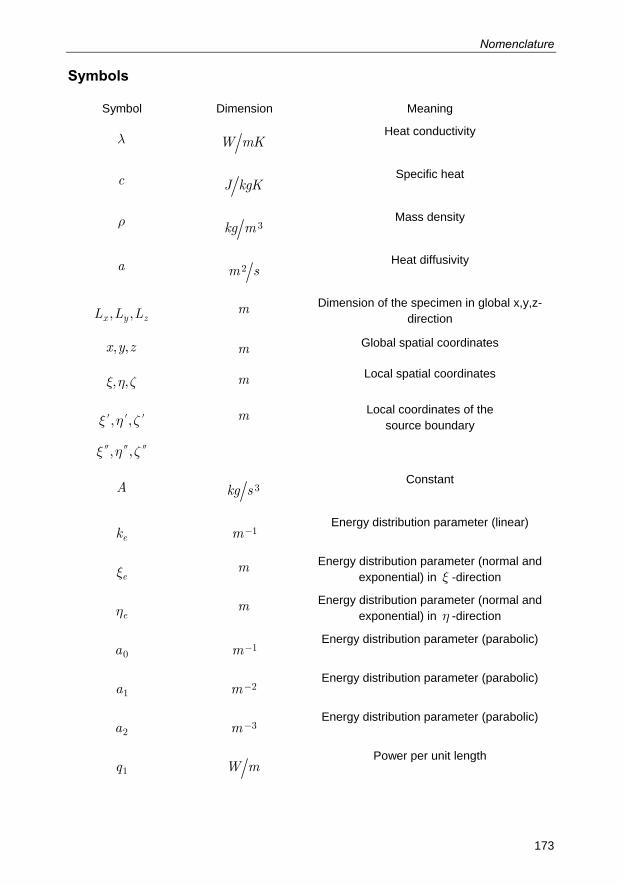
Nomenclature
173
Symbols
Symbol Dimension Meaning
l W mK Heat conductivity
c J kgK Specific heat
r kg m 3 Mass density
a m s2 Heat diffusivity
x y zL L L, , m Dimension of the specimen in global x,y,z-direction
x y z, , m Global spatial coordinates
, ,x h z m Local spatial coordinates
, ,x h z¢ ¢ ¢
, ,x h z
m Local coordinates of the source boundary
A kg s 3 Constant
ek m 1- Energy distribution parameter (linear)
ex m Energy distribution parameter (normal and exponential) in x -direction
eh m Energy distribution parameter (normal and exponential) in h -direction
a0 m 1- Energy distribution parameter (parabolic)
a1 m 2- Energy distribution parameter (parabolic)
a2 m 3- Energy distribution parameter (parabolic)
q1 W m Power per unit length
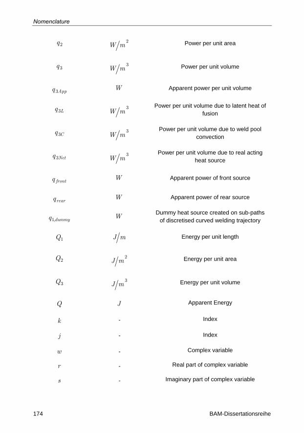
Nomenclature
174 BAM-Dissertationsreihe
q2 W m2
Power per unit area
q3 W m3
Power per unit volume
Appq 3 W Apparent power per unit volume
Lq3 W m3
Power per unit volume due to latent heat of
fusion
Cq3 W m3
Power per unit volume due to weld pool
convection
Netq3 W m3
Power per unit volume due to real acting
heat source
frontq W Apparent power of front source
rearq W Apparent power of rear source
dummyq1, W Dummy heat source created on sub-paths of discretised curved welding trajectory
Q1 J m Energy per unit length
Q2 J m2
Energy per unit area
Q3 J m3
Energy per unit volume
Q J Apparent Energy
k - Index
j - Index
w - Complex variable
r - Real part of complex variable
s - Imaginary part of complex variable
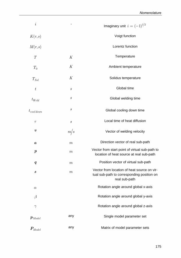
Nomenclature
175
i - Imaginary unit i 1 2( 1)= -
K r s( , ) Voigt function
M r s( , ) Lorentz function
T K Temperature
T0 K Ambient temperature
SolT K Solidus temperature
t s Global time
Weldt s Global welding time
cool downt s Global cooling down time
t s Local time of heat diffusion
v m s Vector of welding velocity
a m Direction vector of real sub-path
p m Vector from start point of virtual sub-path to location of heat source at real sub-path
q m Position vector of virtual sub-path
s m Vector from location of heat source on vir-tual sub-path to corresponding position on
real sub-path
a Rotation angle around global x-axis
b Rotation angle around global y-axis
g Rotation angle around global z-axis
Modelp any Single model parameter set
ModelP any Matrix of model parameter sets
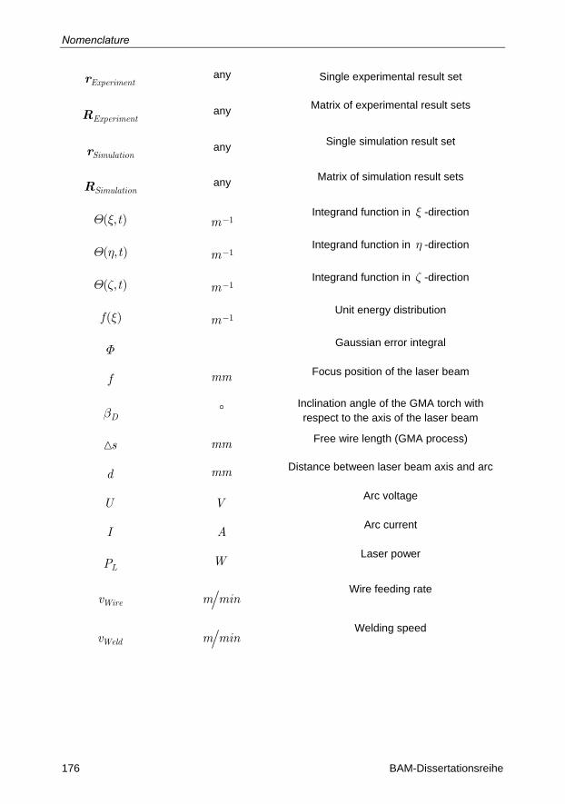
Nomenclature
176 BAM-Dissertationsreihe
Experimentr any Single experimental result set
ExperimentR any Matrix of experimental result sets
Simulationr any Single simulation result set
SimulationR any Matrix of simulation result sets
t( , )Q x m 1- Integrand function in x -direction
t( , )Q h m 1- Integrand function in h -direction
t( , )Q z m 1- Integrand function in z -direction
f ( )x m 1- Unit energy distribution
F Gaussian error integral
f mm Focus position of the laser beam
Db Inclination angle of the GMA torch with respect to the axis of the laser beam
s mm Free wire length (GMA process)
d mm Distance between laser beam axis and arc
U V Arc voltage
I A Arc current
LP W Laser power
Wirev m min Wire feeding rate
Weldv m min Welding speed
177
List of Figures
Fig. 2.1 Coupling of physical domains in welding simulation, ............................................. 4 Fig. 2.2 Overview of computational welding mechanics ..................................................... 8 Fig. 2.3 Physical phenomena of a laser-GMA hybrid welding process ............................... 8 Fig. 2.4 Scatter band of material properties ........................................................................ 9 Fig. 2.5 Overview of errors and uncertainties in simulation ................................................ 9 Fig. 2.6 Classification of parameters for the simulation model ......................................... 10 Fig. 2.7 Apparent heat source model................................................................................ 12 Fig. 2.8 Simplifications and Assumptions of analytical heat conduction models ............... 14 Fig. 2.9 Normal distributed temperature response of an infinite solid, t = 0.5 s ................ 15 Fig. 2.10 Normal distributed temperature response of an infinite solid, t = 1 s ................... 16 Fig. 2.11 Overview of analytical heat source model characteristics ................................... 17 Fig. 2.12. Methodology to solve an inverse problem ........................................................... 20 Fig. 2.13 Objective function of two design variables containing noisy data ........................ 22 Fig. 2.14 Classification of optimisation algorithms .............................................................. 22 Fig. 2.15 Functionality of a single neuron acting as information processing unit ................ 23 Fig. 2.16: Structure of multi-layered feed forward neural network ....................................... 24 Fig. 3.1 Geometry of the specimen used for the conducted experiments ......................... 31 Fig. 3.2 Experimental setup of laser GMA hybrid welding experiments ............................ 32 Fig. 3.3 Configuration of laser beam and GMA torch........................................................ 32 Fig. 3.4: Heat source acting on a finite solid ...................................................................... 34 Fig. 3.5: Exemplary power distribution of volumetric heat source ...................................... 35 Fig. 3.6: Bounded unit energy distribution along the local -axis ....................................... 35 Fig. 3.7 Reference model setup ....................................................................................... 38 Fig. 3.8 Transient behaviour of integrand function ( , , )Q x h z .......................................... 40 Fig. 3.9 Maintaining adiabatic boundary conditions for a bounded heat source ............... 41 Fig. 3.10 Model setup used for comparison of analytical heat source model ..................... 43 Fig. 3.11 Extraction of experimental reference data ........................................................... 44 Fig. 3.12 Cross section and indication of extracted reference points ................................. 47 Fig. 3.13 Thermal cycle at location A and indication of reference point .............................. 47

List of Figures
178 BAM-Dissertationsreihe
Fig. 3.14 Geometry of the fusion line in the cross section .................................................. 48 Fig. 4.1 Comparison of cross sections for hybrid weldments ............................................ 50 Fig. 4.2 Thermal cycle measurements for the hybrid welding experiment ........................ 51 Fig. 4.3 Cross sections for laser beam weldments ........................................................... 51 Fig. 4.4 High speed record of molten pool at the top surface ........................................... 52 Fig. 4.5 Thermal cycle measurements for the laser beam experiment ............................. 52 Fig. 4.6 Thermal cycle measurements for the laser beam experiment ............................. 53 Fig. 4.7: Series development of bounded distributed heat source ..................................... 54 Fig. 4.8: Method to model the stop of action of a heat source ........................................... 56 Fig. 4.9: Separation of normal distribution into front and rear part ..................................... 59 Fig. 4.10 Normal heat source: influence of heat source boundary ..................................... 67 Fig. 4.11 Exponential heat source: influence of heat source boundary .............................. 67 Fig. 4.12 Parabolic heat source: influence of heat source boundary .................................. 68 Fig. 4.13 Influence of normal energy distribution parameter ............................................... 68 Fig. 4.14 Influence of exponential energy distribution parameter ....................................... 69 Fig. 4.15 Influence of parabolic energy distribution parameter a0 ....................................... 69 Fig. 4.16 Influence of parabolic energy distribution parameter a1 ....................................... 70 Fig. 4.17 Influence of parabolic energy distribution parameter a2 ....................................... 70 Fig. 4.18 Transient integrand function for a normal distribution .......................................... 71 Fig. 4.19 Transient integrand function for an exponential distribution ................................ 71 Fig. 4.20 Transient integrand function for a parabolic distribution ...................................... 72 Fig. 4.21 Temperature profile during welding along the weld centre line ............................ 73 Fig. 4.22 Temperature profile during welding along the weld centre line ............................ 74 Fig. 4.23 Temperature profile during cooling down along the weld centre line ................... 74 Fig. 4.24 Temperature profile during cooling down along the weld centre line ................... 75 Fig. 4.25 Thermal cycle recorded at a point on the weld centre line ................................... 75 Fig. 4.26 Thermal cycle recorded at a point on the weld centre line ................................... 76 Fig. 4.27 Approximation of a parabolic energy distribution by a Fourier series .................. 76 Fig. 4.28: Decomposition of welding trajectory into sub-paths ............................................. 77 Fig. 4.29 Algorithm to generate the array of dummy heat sources ..................................... 79 Fig. 4.30 Movement of heat source along the global x - direction ...................................... 81
List of Figures
179
Fig. 4.31 Sketch to visualise the principle of 2D coordinate transformation ........................ 82 Fig. 4.32 Movement on a three dimensional welding trajectory .......................................... 84 Fig. 4.33 Computational and virtual domain due to reflected heat sources ........................ 85 Fig. 4.34 Temperature contours on top surface at time 24 s .............................................. 86 Fig. 4.35 Temperature contours on top surface at time 24 s .............................................. 86 Fig. 4.36 Temperature contours on top surface at time 24 s .............................................. 87 Fig. 4.37 Analytically calculated temperature field at the top surface (t = 16 s) .................. 87 Fig. 4.38 Analytically calculated temperature field at the top surface (t = 21 s) .................. 88 Fig. 4.39 Thermal cycles at the top surface calculated analytically .................................... 88 Fig. 4.40 Projection of the 3D isosurface of the solidus temperature ................................. 89 Fig. 4.41 Search algorithm to determine the maximum weld pool width ............................. 90 Fig. 4.42 Determination of location of molten zone ............................................................ 91 Fig. 4.43 Algorithm for evaluation of the fusion line in the cross section ............................ 93 Fig. 4.44 Contour of weld pool width evaluated at the top surface ..................................... 94 Fig. 4.45 Contour of weld pool width evaluated at the bottom surface ............................... 95 Fig. 4.46 Contour of the weld pool depth ............................................................................ 96 Fig. 4.47 Contour of the weld pool length evaluated at the top surface .............................. 96 Fig. 4.48 Objective function calculated for case a) ............................................................. 97 Fig. 4.49 Objective function calculated for case b) ............................................................. 98 Fig. 4.50 Objective function calculated for case c) ............................................................. 99 Fig. 4.51 Objective function calculated for case d) ........................................................... 100 Fig. 4.52 Calculated thermal cycles for the reference parameters ................................... 100 Fig. 4.53 Random selection of model parameter sets ...................................................... 102 Fig. 4.54 Training of preliminary neural network ............................................................... 102 Fig. 4.55 Movement of local domain of model parameters ............................................... 103 Fig. 4.56 Evaluation of global minimum by means of neural network ............................... 104 Fig. 4.57 Evaluation of global minimum by means of neural network ............................... 105 Fig. 4.58 Evaluation of global minimum by means of neural network ............................... 106 Fig. 4.59 Convergence behaviour of the heat source power ............................................ 107 Fig. 4.60 Convergence behaviour of the energy distribution parameter re,xy ..................... 108 Fig. 4.61 Convergence behaviour of the energy distribution parameter e ....................... 108
List of Figures
180 BAM-Dissertationsreihe
Fig. 4.62 Convergence behaviour of the heat source power ............................................ 109 Fig. 4.63 Convergence behaviour of the energy distribution parameter re,xy ..................... 110 Fig. 4.64 Convergence behaviour of the energy distribution parameter e ....................... 110 Fig. 4.65 Convergence behaviour of the heat source power ............................................ 111 Fig. 4.66 Convergence behaviour of the energy distribution parameter re,xy ..................... 112 Fig. 4.67 Convergence behaviour of the energy distribution parameter e ....................... 112 Fig. 4.68 Convergence behaviour of top and bottom net heat input per time ................... 114 Fig. 4.69 Convergence behaviour of energy distribution parameters ............................... 114 Fig. 4.70 Calculated fusion line in the cross section ......................................................... 115 Fig. 4.71 Calculated thermal cycles at the top surface ..................................................... 115 Fig. 4.72 Calculated thermal cycles at the bottom surface ............................................... 116 Fig. 4.73 Calculated temperature contour at the top surface ............................................ 116 Fig. 4.74 Derivation of the heat source energy distribution............................................... 118 Fig. 4.75 Convergence behaviour of the net heat input per time for a line source ............ 120 Fig. 4.76 Convergence behaviour of the net heat input per time ...................................... 121 Fig. 4.77 Convergence behaviour of normal energy distribution parameter r
e,xy ................. 121
Fig. 4.78 Calculated fusion line in the cross section for a single heat source ................... 122 Fig. 4.79 Calculated thermal cycles at the top surface for a single heat source ............... 122 Fig. 4.80 Calculated thermal cycles at the bottom surface ............................................... 123 Fig. 4.81 Convergence behaviour of net heat input per time ............................................ 124 Fig. 4.82 Calculated fusion line (cross section) for the laser GMA hybrid welding ........... 125 Fig. 4.83 Calculated thermal cycles for the laser GMA hybrid welding ............................. 126 Fig. 4.84 Calculated temperature field for laser GMA hybrid welding ............................... 126 Fig. 5.1 Comparison of different energy distributions ..................................................... 128 Fig. 5.2 Comparison of integrand function of different energy distributions .................... 130 Fig. 5.3 Temperature profile during welding along the weld centre line .......................... 131 Fig. 5.4 Temperature profile during cooling down along the weld centre line ................. 131 Fig. 5.5 Thermal cycle recorded at a point on the weld centre line ................................. 132 Fig. 5.6 Temperature profile along the measuring path at time t = 16 s ......................... 135 Fig. 5.7 Temperature profile along the measuring path at time t = 21 s ......................... 136 Fig. 5.8 Comparison of thermal cycles that are calculated analytically ........................... 136
List of Figures
181
Fig. 5.9 Top weld pool width plotted against the radius .................................................. 140 Fig. 5.10 Sensitivity of bottom weld pool width ................................................................. 141 Fig. 5.11 Objective function for case a) ............................................................................ 142 Fig. 5.12 Objective function for case c) ............................................................................ 143 Fig. 5.13 Random selection of model parameter sets ...................................................... 145 Fig. 5.14 Random selection of model parameter sets ...................................................... 146 Fig. 5.15 Neural network optimisation algorithm in the vicinity of the minimum ................ 147 Fig. 5.16 Neural network optimisation algorithm in the vicinity of the minimum ................ 149 Fig. 5.17 Neural network optimisation algorithm ............................................................... 149 Fig. 5.18 Simulated fusion lines in the cross section for the repeated calibration ............. 151 Fig. 5.19 Comparison of weld pool lengths at the top surface .......................................... 151 Fig. 5.20 Calculated thermal cycles at point A for the repeated calibration runs .............. 152 Fig. 5.21 Simulated fusion lines in the cross section for the repeated calibration ............. 152 Fig. 5.22 Calculated thermal cycles at point A for the repeated calibration ...................... 153 Fig. 5.23 Simulated fusion lines in the cross section for the repeated calibration ............. 155 Fig. 5.24 Calculated thermal cycles at point A for the repeated calibration ...................... 155 Fig. 5.25 Random selection of values for net heat input during calibration....................... 157 Fig. 5.26 Random selection of energy distribution parameters during calibration ............ 158 Fig. 5.27 Comparison of calculated and experimental fusion line ..................................... 159 Fig. 5.28 Comparison of calculated and experimental thermal cycles .............................. 159 Fig. 5.29 Comparison of calculated and experimental thermal cycles .............................. 160 Fig. 5.30 Comparison of calculated and experimental geometry of the weld pool ............ 160 Fig. 5.31 Random selection of values for net heat input during calibration....................... 161 Fig. 5.32 Random selection of energy distribution parameters during calibration ............ 162 Fig. 5.33 Comparison of fusion line due to the superposition ........................................... 163 Fig. 5.34 Comparison of calculated and experimental thermal cycles .............................. 163 Fig. 5.35 Comparison of calculated and experimental thermal cycles .............................. 164 Fig. 5.36 Comparison of calculated and experimental fusion line ..................................... 165 Fig. 5.37 Comparison of calculated and experimental thermal cycles .............................. 166 Fig. 5.38 Comparison of calculated and experimental shape of top weld pool ................. 166
182 BAM-Dissertationsreihe
List of Tables
Table 3.1 Chemical composition of the S355J2+N .............................................................. 31 Table 3.2 Overview of selected experiments for the temperature field calibration ............... 33 Table 3.3 Thermo physical material properties of S355J2+N .............................................. 37 Table 3.4 Overview of parameter variations for the heat source boundary ......................... 38 Table 3.5 Overview of heat source parameter variations .................................................... 39 Table 3.6 Overview of parameter variations for the heat source boundary ......................... 39 Table 3.7 Overview of heat source parameters ................................................................... 41 Table 4.1 Selected instances of time for the extraction of temperature values .................. 101 Table 5.1 Comparison of computational time between ...................................................... 137 Table 5.2 Comparison of distances to the welding centre line ........................................... 158 Table 5.3 Comparison of distances to the welding centre ................................................. 165
183
Literature
[1] Rykalin, N. N., "Die Wärmegrundlagen des Schweißvorganges", Berlin, Verlag Technik, 1952.
[2] Rosenthal, D., "Mathematical Theory of Heat Distribution During Welding and Cutting", Welding Research-Supplement to the Welding Journal, vol. 20 (5), pp. 220-s-234-s, 1941
[3] Rosenthal, D., "The Theory of Moving Sources of Heat and its Application to Metal Treatments", Transactions of the A.S.M.E., vol. 68, pp. 849-866, 1946
[4] Goldak, J. A., Akhlaghi, M., "Computational Welding Mechanics", New York, Springer, 2005.
[5] Radaj, D., "Welding Residual Stresses and Distortion: Calculation and Measurement", 2. edition, Düsseldorf, DVS-Verlag, 2003.
[6] Radaj, D., "Schweißprozeßsimulation: Grundlagen und Anwendungen", Düsseldorf, DVS-Verlag, 1999.
[7] Lindgren, L. E., "Finite Element Modelling and Simulation of Welding, Part 2: Improved Material Modelling", Journal of Thermal Stresses, vol. 24 (3), pp. 195-231, 2001
[8] Zacharia, T., Vitek, J. M., Goldak, J. A., DebRoy, T., Rappaz, M., Bhadeshia, H. K. D. H., "Modelling of Fundamental Phenomena in Welds", Modelling and Simulation in Materials Science and Engineering, vol. 3 (2), pp. 265-288, 1995
[9] Ferro, P., Bonollo, F., Tiziani, A., Magnabosco, I., "A Review of Welding Process Numerical Simulation: Methodologies and Experimental Validations", in 2nd International Conference and Exhibition on New Developments in Metallurgical Process Technology, 2004, Riva del Garda, Italy, 19-21 September 2004
[10] Grong, O., "Metallurgical Modelling of Welding", Materials Modelling Series, 2. edition, London, UK, The Institute of Materials, 1997.
[11] Carslaw, H. S., Jaeger, J. C., "Conduction of Heat in Solids", Cambridge, UK, Oxford University Press, 1959.
[12] Wilson, H. A., "On Convection of Heat", Proceedings of the Cambridge Philosophical Society, vol. 12, pp. 406-423, 1904
Literature
184 BAM-Dissertationsreihe
[13] Roberts, O. F. T., "The Theoretial Scattering of Smoke in a Turbulent Atmosphere", Proceedings of the Royal Society (London), vol. A104, pp. 640-655, 1923
[14] Mazumder, J., Mohanty, P. S., Kar, A., "Mathematical Modelling of Laser Materials Processing", International Journal of Materials and Product Technology, vol. 11 (3), pp. 193-252, 1996
[15] Bailey, C., "Discretisation Procedures for Multi-Physics Phenomena", Computational and Applied Mathematics, vol. 103 (1), pp. 3-17, 1999
[16] Cho, M. H., Farson, D. F., "Simulation Study of a Hybrid Process for the Prevention of Weld Bead Hump Formation", Welding Research-Supplement to the Welding Journal, vol. 86 (9), pp. 253-s-262-s, 2007
[17] Hu, J., Tsai, H. L., "Heat and Mass Transfer in Gas Metal Arc Welding. Part I: The Arc", International Journal of Heat and Mass Transfer, vol. 50 (5-6), pp. 833-846, 2007
[18] Schnick, M., Munoz, J. E. F., Fuessel, U., "Experimental Possibilities of Gas Tungsten Arc Analysis", Welding and Cutting, vol. 6 (5), pp. 282-287, 2007
[19] Yamamoto, K., Tanaka, M., Tashiro, S., Nakata, K., Murphy, A. B., "Numerical Simulation of Metal Vapor Behaviour in Argon TIG Welding", Transactions of Joining and Welding Research Institute, Osaka University, vol. 36 (2), pp. 1-4, 2007
[20] Cao, Z., Yang, Z., Chen, X. L., "Three-Dimensional Simulation of Transient GMA Weld Pool with Free Surface", Welding Research-Supplement to the Welding Journal, vol. 83 (6), pp. 169-s-176-s, 2004
[21] Zhao, Y. Z., Zhao, H. Y., Lei, Y. P., Shi, Y. W., "Theoretical Study of Marangoni Convection and Weld Penetration under Influence of High Oxygen Content in Base Metal", Science and Technology of Welding and Joining, vol. 12 (5), pp. 410-417, 2007
[22] Mahrle, A., Weiss, D., "Simulation of Temperature Fields in Arc and Beam Welding", Heat and Mass Transfer, vol. 36 (2), pp. 117-126, 2000
[23] Sudnik, W., Radaj, D., W., E., "Computerized Simulation of Laser Beam Welding, Modelling and Verification", Journal of Physics D: Applied Physics, vol. 29 (11), pp. 2811-2817, 1996
[24] Mazumder, J., Steen, W. M., "Heat Transfer Model for cw Laser Material Processing", Journal of Applied Physics, vol. 51 (2), pp. 941-947, 1980
Literature
185
[25] Lampa, C., Kaplan, A., Powel, J., Magnusson, C., "An Analytical Thermodynamic Model of Laser Welding", Journal of Physics D: Applied Physics, vol. 30 (9), pp. 1293-1299, 1997
[26] Zhou, J., Tsai, H. L., "Effects of Electromagnetic Force on Melt Flow and Porosity Prevention in Pulsed Laser Keyhole Welding", International Journal of Heat and Mass Transfer, vol. 50 (11-12), pp. 2217-2235, 2006
[27] Seyffarth, P., Krivtsun, I. V., "Laser-Arc Processes and their Applications in Welding and Material Treatment", Welding and Allied Processes, New York, Taylor & Francis, 2002.
[28] Gumenyuk, A., "Modellbildung und Prozesssimulation des Laserstrahlschweißens von Leichtbauwerkstoffen", Ph.D. thesis, Fakultät für Maschinenwesen, Rheinisch-Westfälisch Technische Hochschule (RWTH), Aachen, 2004.
[29] Sudnik, W., Radaj, D., Breitschwerdt, S., Erofeev, W., "Numerical Simulation of Weld Pool Geometry in Laser Beam Welding", Journal of Physics D: Applied Physics, vol. 33 (6), pp. 662-671, 2000
[30] Dilthey, U., Gumenyuk, A., Olschok, S., "Hydrodynamische Prozessanalyse beim Laserstrahl-MSG-Hybridschweißverfahren – Teil 3: Prozesssimulation und Vergleich mit Schweißversuchen", Schweißen und Schneiden, vol. 60 (3), pp. 151-155, 2008
[31] Otto, A., "Transiente Prozesse beim Laserstrahlschweißen", Ph.D. thesis, Technische Fakultät, Friedrich-Alexander-Universität Erlangen-Nürnberg, 1997.
[32] Janssens, K., Frans, G., Raabe, D., Nestler, B., Kozeschnik, E., Miodownik, M. A., "Computational Materials Engineering: An Introduction to Microstructure Evolution", Amsterdam, Elsevier Academic Press, 2007.
[33] Babu, S. S., "Thermodynamic and Kinetic Models for Describing Microstructure Evolution During Joining of Metals and Alloys", International Materials Reviews, vol. 54 (6), pp. 333-367, 2009
[34] Vitek, J. M., "Modelling and Simulation of Micro Structural Development During Weld Solidification", in Mathematical Modelling of Weld Phenomena 5, Ed.: Cerjak, H., Bhadeshia, H. K. D. H., Maney Publishing, pp. 82-98, 2001
[35] Rappaz, M., "Modelling of Microstructure Formation in Solidification Processes", International Materials Reviews, vol. 34 (1), pp. 93-124, 1989
[36] Zhang, W., Elmer, J. W., DebRoy, T., "Integrated Modelling of Thermal Cycles, Austenite Formation, Grain Growth and Decomposition in the Heat Affected Zone of Carbon Steel", Science and Technology of Welding and Joining, vol. 10 (5), pp. 574-582, 2005
Literature
186 BAM-Dissertationsreihe
[37] Rayamaki, P., Karkhin, V. A., Khomich, P. N., "Determination of the Main Characteristics of the Temperature Field for the Evaluation of the Type of Solidification of Weld Metal in Fusion Welding", Welding International, vol. 21 (8), pp. 600-604, 2007
[38] Karkhin, V. A., Khomich, P. N., Rayamaki, P., "Analysis of Chemical Macroheterogeneity in the Vicinity of the Fusion Boundary in Fusion Welding", Welding International, vol. 24 (2), pp. 125 - 130, 2010
[39] Haidemenopoulos, G. N., "Coupled Thermodynamic/Kinetic Analysis of Diffusional Transformations during Laser Hardening and Laser Welding", Journal of Alloys and Compounds, vol. 320 (2), pp. 302-307, 2001
[40] Holzer, I., Mayr, P., Sonderegger, B., Kozeschnik, E., Cerjak, H., "Simulation and Validation of the Evolution of Precipitates During Production and Fabrication of a Complex Martensitc 9wt. % Cr Steel", in 17th International Conference on Computer Technology in Welding and Manufacturing, TWI Ltd, pp. 1-10, Cranfield University, UK, 18-19 June 2008
[41] Myhr, O. R., Grong, O., "Utilizing a Predictive Tool for Designing Welded Aluminium Components", Welding Journal, vol. 87 (5), pp. 36-39, 2008
[42] Guo, W., Kar, A., "Determination of Weld Pool Shape and Temperature Distribution by Solving Three-Dimensional Phase Change Heat Conduction Problem", Science and Technology of Welding and Joining, vol. 5 (5), pp. 317-323, 2000
[43] Thiessen, R. G., Richardson, I. M., "A Strategy for Modeling Microstructure in Macroscopic Simulations of Welded Material", Metallurgical and Materials Transactions B, vol. 37 (2), pp. 293-299, 2006
[44] Ploshikhin, V., Zoch, H.-W., Karkhin, V. A., Pesch, H.-J., Diepers, H.-J., Steinbach, I., "Multiscale Modelling of Laser Beam Welding, Part I: Macroscopic and Mesoscopic Scale", Kurzzeitmetallurgie Strahltechnik Band 18, BIAS Verlag, Bremen, 2002
[45] Karkhin, V. A., Ploshikhin, V., Bermann, H., "Solution of Inverse Heat Conduction Problem for Determining Heat Input, Weld Shape and Grain Structure During Laser Welding", Science and Technology of Welding and Joining, vol. 7 (4), pp. 224-231, 2001
[46] Böllinghaus, T., Herold, T., "Hot Cracking Phenomena in Welds I", First International Workshop - March 2004, Berlin, Springer, 2005.
[47] Böllinghaus, T., Herold, T., "Hot Cracking Phenomena in Welds II", Second International Workshop - March 2007, Berlin, Springer, 2008.
Literature
187
[48] Koistinen, D. P., Marburger, R. E., "A General Equation Prescribing the Extent of a Austenite-Martensite Transformation in Pure Iron-Carbon Alloys and Plain Carbon Steels", Acta Metallurgica, vol. 7 1959
[49] Leblond, J. B., "A new Kinetic Model for Anisothermal Matllurgical Transformations in Steels including Effect of Austenite Grain Size", Acta Metallurgica, vol. 32 (1), pp. 137–146, 1984
[50] Leblond, J. B., Pont, D., Devaux, J., Nru, D., Bergheau, J. M., "Metallurgical and Mechanical Consequences of Phase Transformations in Numerical Simulation of Welding Processes", in Modelling In Welding, Hot Powder Forming and Casting, ASM International, pp. 61-81, 1997, Materials Park, Ohio, 1997
[51] Wohlfahrt, H., Macherauch, E., "Die Ursachen des Schweißeigenspannungszustandes", Materialprüfung, vol. 19 (8), pp. 272-280, 1977
[52] Wohlfahrt, H., Macherauch, E., "Die Bedeutung der Austenitumwandlung für die Eigenspannungsentstehung beim Schweißen", Härterei Technische Mitteilungen, vol. 41 (5), pp. 248-257, 1986
[53] Nitschke-Pagel, T. N., Dilger, K., "Eigenspannungen in Schweißverbindungen - Teil 1: Ursachen der Eigenspannungsentstehung beim Schweißen", Schweißen und Schneiden, vol. 58 (9), pp. 466-479, 2006
[54] Nitschke-Pagel, T. N., Dilger, K., "Eigenspannungen in Schweißverbindungen - Teil 3: Verringerung von Eigenspannungen", Schweißen und Schneiden, vol. 59 (7), pp. 387-395, 2007
[55] Nitschke-Pagel, T. N., Dilger, K., "Eigenspannungen in Schweißverbindungen - Teil 2: Bewertung von Eigenspannungen", Schweißen und Schneiden, vol. 59 (1), pp. 23-32, 2007
[56] Bergheau, J. M., Vincent, Y., Leblond, J. B., Jullien, J. F., "Viscoplastic Behaviour of Steels During Welding", Science and Technology of Welding and Joining, vol. 9 (4), pp. 323-330, 2004
[57] Doynov, N., Ossenbrink, R., Schmidt, J., Michailov, V., "Utilization of Weld Pool Models in Thermal-Mechanical Simulations", in Mathematical Modelling of Weld Phenomena 8, Ed.: Cerjak, H., Bhadeshia, H. K. D. H., Kozeschnik, E., Verlag der Technischen Universität Graz, pp. 925-938, 2007
[58] Mochizuki, M., Yamasaki, H., Okano, S., Toyoda, M., "Distortion Behaviour of Fillet T-joint During In-Process Control Welding by Additional Cooling", Welding in the World, vol. 50 (5-6), pp. 46-50, 2006
Literature
188 BAM-Dissertationsreihe
[59] Pavlyk, V., Mokrov, O., Dilthey, U., "Heat Source Modelling in GMA-Welding and its Integration in Stress-Strain Analysis", in Mathematical Modelling of Weld Phenomena 8, Ed.: Cerjak, H., Bhadeshia, H. K. D. H., Kozeschnik, E., Verlag der Technischen Universität Graz, pp. 801-818, 2007
[60] Schwenk, C., Rethmeier, M., Dilger, K., Michailov, V., "Schweißsimulation im Fahrzeugbau - Möglichkeiten, Grenzen und Herausforderungen", DVS-Bericht, vol. 237, pp. 353–358, 2005
[61] Schwenk, C., "FE-Simulation des Schweißverzugs laserstrahlgeschweißter dünner Bleche - Sensitivitätsanalyse durch Variation der Werkstoffkennwerte", Ph.D. thesis, Fakultät V - Verkehrs- und Maschinensysteme, Technische Universität Berlin, 2007.
[62] Heinze, C., Caron, J., Schwenk, C., Rethmeier, M., Lippold, J., Babu, S., "Sensitivity Analysis of Martensite Transformation Temperatures with respect to Numercial Calculation of Welding-Induced Residual Stresses", in Mathematical Modelling of Weld Phenomena 9, Ed.: Cerjak, H., Enzinger, N., Verlag der Technischen Universität Graz, pp. 215-238, 2010
[63] Lindgren, L. E., "Modelling for Residual Stresses and Deformations due to Welding - Knowing What isn’t Necessary to Know", in Mathematical Modelling of Weld Phenomena 6, Ed.: Cerjak, H., Bhadeshia, H. K. D. H., Maney Publishing, pp. 491–518, 2002
[64] Sakkiettibutra, J., Loose, T., Wohlfahrt, H., "New 3D-Calculations of Residual Stresses Consistent with Measured Results of the IIW Round Robin Programme", in Mathematical Modelling of Weld Phenomena 9, Ed.: Cerjak, H., Enzinger, N., Verlag der Technischen Universität Graz, pp. 369-390, 2010
[65] Schenk, T., Richardson, I. M., Kraska, M., Ohnimus, S., "Influence of Clamping on Distortion of Welded S355 T-Joints", Science and Technology of Welding and Joining, vol. 14 (4), pp. 369-375, 2009
[66] Mollicone, P., Camilleri, D., Gray, T. G. F., Comlekci, T., "Simple Thermo-Elastic–Plastic Models for Welding Distortion Simulation", Journal of Materials Processing Technology, vol. 176 (1-3), pp. 77–86, 2006
[67] Stapelfeld, C., Kloshek, A., Doynov, N., Michailov, V. G., "Analytisches Schrumpfkraftmodell und Berechnungsprogramm zur Bestimmung des schweißbedingten Verzugs", DVS-Berichte, vol. 250, pp. 401-405, 2008
[68] Ploshikhin, V., "Methode und Software zur effizienten Berechnung der Schweißverzüge an Großbauteilen", Abschlussbericht zum Verbundvorhaben "Intelligente Softwarelösung zur schnellen Vorhersage und Optimierung von Schweißverzügen bei der Entwicklung von Großbauteilen (INSOFT)", DVS Media, Düsseldorf, DVS-Bericht 259, 2009.
Literature
189
[69] Perret, W., Thater, R., Alber, U., Schwenk, C., Rethmeier, M., "Case Study for Welding Simulation in the Automotive Industry", IIW Doc. SC-Auto-37-10, pp. 1-13, 2010
[70] Patankar, S., "Numerical Heat Transfer and Fluid Flow", Series in Computational Methods in Mechanics and Thermal Sciences, Bristol, PA, Taylor & Francis, 1980.
[71] Versteeg, H. K., Malalasekera, W., "An Introduction to Computational Fluid Dynamics - the Finite Volume Method ", New York, Wiley, 1995.
[72] Weiss, D., Christensen, K. H., Kristensen, J. K., "Computerised Calibration of Thermal Welding Models", in Mathematical Modelling of Weld Phenomena 8, pp. 469-484, 2007
[73] Kogel-Hollacher, M., "Sensorik und Datenauswertung zur industriellen Prozessüberwachung beim Laserstrahlschweißen", Ph.D. thesis, Fakultät II - Mathematik und Naturwissenschaften, Technische Universität Berlin, 2008.
[74] Müller, M. G., "Prozessüberwachung beim Laserstrahlschweißen durch Auswertung der reflektierten Strahlung", Ph.D. thesis, Institut für Strahlwerkzeuge (IFSW), Universität Stuttgart, 2002.
[75] Stelling, K., "Laserstrahl-Plasma-Hybridschweißen austenitischer Stähle", Ph.D. thesis, Fakultät V - Verkehrs- und Maschinensysteme, Technische Universität Berlin, 2008.
[76] Schwenk, C., Rethmeier, M., Dilger, K., Michailov, V., "Sensitivity Analysis of Welding Simulation Depending on Material Properties Value Variation", in Mathematical Modelling of Weld Phenomena 8, Ed.: Cerjak, H., Bhadeshia, H. K. D. H., Kozeschnik, E., Verlag der Technischen Universität Graz, pp. 1107-1128, 2007
[77] Sudnik, W., Radaj, D., Erofeev, W., "Validation of Computerised Simulation of Welding Processes", in Mathematical Modelling of Weld Phenomena 4, Ed.: Cerjak, H., Bhadeshia, H. K. D. H., Maney Publishing, pp. 477-493, 1998
[78] Radaj, D., Lindgren, L. E., "Verification and Validation in Computational Welding Mechanics", in Mathematical Modelling of Weld Phenomena 8, Ed.: Cerjak, H., Bhadeshia, H. K. D. H., Kozeschnik, E., Verlag der Technischen Universität Graz, pp. 1039-1051, 2007
[79] Richter, F., "Stahleisen-Sonderberichte. Bd. 8: Die wichtigsten physikalischen Eigenschaften von 52 Eisenwerkstoffen", Düsseldorf, Verlag Stahleisen mbH, 1973.
Literature
190 BAM-Dissertationsreihe
[80] Weiss, D., Christensen, K. H., Kristensen, J. K., "Acceleration of Numerical Solution of Inverse Problems in Gas Metal Arc Welding", in 14th International Conference on Computer Technology in Welding and Manufacturing, TWI Ltd, pp. 1-10, 2004, Sheffield Hallam University, UK, 16 - 17 June 2004
[81] Trucano, T. G., Swiler, L. P., Igusa, T., Oberkampf, W. L., Pilch, M., "Calibration, Validation and Sensitivity Analysis: What’s What", Reliability Engineering System Safety, vol. 91 (10-11), pp. 1331-1357, 2006
[82] Asserin, O., Loredo, A., Petelet, M., Iooss, B., "Global Sensitivity Analysis in Welding Simulations — What are the Material Data You Really Need ?", Finite Elements in Analysis and Design, vol. 47, pp. 1004-1016, 2011
[83] Saltelli, A., Ratto, M., Andres, T., Campolongo, F., Cariboni, J., Gatelli, D. M., Saisana, T. S., "Global Sensitivity Analysis - The Primer", New York, Wiley, 2008.
[84] Goldak, J., Bibby, M., Moore, J., House, R., Patel, B., "Computer Modeling of Heat Flow in Welds", Metallurgical and Materials Transactions B, vol. 17 (3), pp. 587-600, 1986
[85] Bag, S., Trivedi, A., De, A., "Development of a Finite Element Based Heat Transfer Model for Conduction Mode Laser Spot Welding Process Using an Adaptive Volumetric Heat Source", International Journal of Thermal Sciences, vol. 48 (10), pp. 1923-1931, 2009
[86] Kumar, A., DebRoy, T., "Guaranteed Fillet Weld Geometry from Heat Transfer Model and Multivariable Optimization", International Journal of Heat and Mass Transfer, vol. 47 (26), pp. 5793-5806, 2004
[87] van Elsen, M., Baelmans, M., Mercelis, P., Kruth, J.-P., "Solutions for Modelling Heat Sources in a Semi-Infinite Medium and Applications to Laser Material Processing", International Journal of Heat and Mass Transfer, vol. 50 (23-24), pp. 4872-4882, 2007
[88] De, A., Maiti, S. K., Walsh, C. A., Bhadeshia, H. K. D. H., "Finite Element Simulation of Laser Spot Welding", Science and Technology of Welding and Joining, vol. 8 (5), pp. 377-384, 2003
[89] Prokhorov, N., "A General Equation for the Surface of the Solidification Front During Welding (in Russian)", Svar. Proiz. , vol. 2, pp. 1-4, 1969
[90] Karkhin, V. A., Khomich, P. N., Michailov, V. G., "Models for Volume Heat Sources and Functional-Analytical Technique for Calculating the Temperature Fields in Butt-Welding", in Mathematical Modelling of Weld Phenomena 8, Ed.: Cerjak, H., Bhadeshia, H. K. D. H., Kozeschnik, E., Verlag der Technischen Universität Graz, pp. 819-834, 2007
Literature
191
[91] Lindgren, L. E., "Finite Element Modelling and Simulation of Welding, Part 3: Efficiency and Integration", Journal of Thermal Stresses, vol. 24 (4), pp. 305-334, 2001
[92] Reddy, J. N., "An Introduction to the Finite Element Method", McGraw-Hill Series in Mechanical Engineering, Oxford, UK, Oxford University Press, 2006.
[93] Goldak, J., Chakravarti, A., Bibby, M., "A New Finite Element Model for Welding Heat Sources", Metallurgical and Materials Transactions B, vol. 15 (2), pp. 299-305, 1984
[94] Zhang, J., Dong, Y., "Method for Determining a Heat Source Model for a Weld", United States Patent US 6324491 B1, November, 27, 2001.
[95] Komanduri, R., Hou, Z. B., "Thermal Analysis of the Arc Welding Process: Part I. General Solutions", Metallurgical and Materials Transactions B, vol. 31 (6), pp. 1353-1370, 2000
[96] Beck, J. V., Cole K.D., HajiI-Sheikh A., Litkouhi, B., "Heat Conduction Using Green’s Functions", Series in Computational and Physical Processes in Mechanics and Thermal Sciences, London, Washington, Philadelphia, Hemisphere Publishing Corporation, 1992.
[97] Pilipenko, A., "Computer Simulation of Residual Stress and Distortion of Thick Plates in Multi-Electrode Submerged Arc Welding – Their Mitigation Techniques", Ph.D. thesis, Department of Machine Design and Materials Technology, Norwegian University of Science and Technology, Trondheim, Norway, 2001.
[98] Kasuya, T., Yurioka, N., "Analysis of Three Dimensional Heat Conduction in Welding by Dispersed Point Heat Sources", IIW Doc. IX-1554-89, pp. 1-24, 1989
[99] Kasuya, T., Yurioka, N., "Prediction of Wlding Termal Hstory by a Cmprehensive Solution", Welding Research-Supplement to the Welding Journal, vol. 72 (3), pp. 107-s-115-s, 1993
[100] Nunes, A. C., "An Extended Rosenthal Weld Model", Welding Research-Supplement to the Welding Journal, vol. 62 (6), pp. 165-s-170-s, 1983
[101] Eager, W., Tsai, N. S., "Temperature Fields Produced by Travelling Distributed Heat Sources", Welding Research-Supplement to the Welding Journal, vol. 62 (12), pp. 346-s-355-s, 1983
[102] Kwon, Y., Weckman, D. C., "Analytical Thermal Model of Conduction Mode Double Sided Arc Welding", Science and Technology of Welding and Joining, vol. 13 (6), pp. 539-549, 2008
Literature
192 BAM-Dissertationsreihe
[103] Hou, Z. B., Komanduri, R., "General Solutions for Stationary/Moving Plane Heat Source Problems in Manufacturing and Tribology", International Journal of Heat and Mass Transfer, vol. 43 (10), pp. 1679-1698, 2000
[104] Komanduri, R., Hou, Z. B., "Unified Approach and Interactive Program for Thermal Analysis of Various Manufacturing Processes with Application to Machining", Machining Science and Technology: An International Journal, vol. 13 (2), pp. 143-176, 2009
[105] Ravi, V. P., Li, W. B., Easterling, K. E., "Heat Flow Model for Pulsed Welding", Materials Science and Technology, vol. 7 (7), pp. 649-659, 1991
[106] Karkhin, V. A., Michailov, V., Akatsevich, V. D., "Modelling the Thermal Behaviour of Weld and Heat-Affected Zone During Pulsed Power Welding", in Mathematical Modelling of Weld Phenomena 4, Ed.: Cerjak, H., Bhadeshia, H. K. D. H., Maney Publishing, pp. 411-426, 1998
[107] Michailov, V. G., "Erweiterte analytische Modelle für die Berechnung der Temperaturfelder beim Schweißen", DVS-Berichte, vol. 209, pp. 181-186, 2000
[108] Karkhin, V. A., Khomich, P. N., "Minimisation of Heat Input in Pulsed Welding", Welding International, vol. 21 (3), pp. 227-330, 2007
[109] Bertram, L. A., "A Digital Rykalin Function for Welding", Available: http://airex.tksc.jaxa.jp/pl/dr/19970033311/en, (Accessed: 2010-07-04)
[110] Ranatowski, E., Pocwiardowski, A., "An Analytic-Numerical Evaluation of the Thermal Cycle in the HAZ during Welding", in Mathematical Modelling of Weld Phenomena 4, Ed.: Cerjak, H., Bhadeshia, H. K. D. H., Maney Publishing, pp. 379-395, 1998
[111] Ranatowski, E., Pocwiardowski, A., "An Analytic-Numerical Estimation of the Thermal Cycle during Welding with various Heat Source Models Application", in Mathematical Modelling of Weld Phenomena 5, Ed.: Cerjak, H., Bhadeshia, H. K. D. H., Maney Publishing, pp. 725-742, 2001
[112] Ranatowski, E., Pocwiardowski, A., "An Analytical-Numerical Assessment of the Thermal Cycle in HAZ with three Dimensional Heat Source Models and Pulsed Power Welding", in Mathematical Modelling of Weld Phenomena 7, Ed.: Cerjak, H., Bhadeshia, H. K. D. H., Kozeschnik, E., Verlag der Technischen Universität Graz, pp. 1111-1128, 2005
[113] Zhu, X. K., Chao, Y. J., "Effects of Temperature Dependent Material Properties on Welding Simulation", Computers and Structures, vol. 80 (11), pp. 967-976, 2002
Literature
193
[114] Karkhin, V. A., Ilin, A., Ploshikhin, V., Prihodovsky, A., "Effect of the Heat of Melting and Solidification on the Thermal Efficiency of the Melting Process", Welding International, vol. 19 (3), pp. 212-216, 2005
[115] Karkhin, V. A., Pesh, H. J., Ilin, A., Prihodovsky, A., Ploshikhin, V., Makhutin, M. V., Zoch, H.-W., "Effects of Latent Heat of Fusion on Thermal Processes During Welding", in Mathematical Modelling of Weld Phenomena 7, Ed.: Cerjak, H., Bhadeshia, H. K. D. H., Kozeschnik, E., Verlag der Technischen Universität Graz, pp. 39-62, 2005
[116] Ramirez, A. J., Brandi, S. D., "Application of Discrete Distribution Point Heat Source Model to Simulate Multipass Weld Thermal Cycles in Medium Thick Plates", Science and Technology of Welding and Joining, vol. 9 (1), pp. 72-82, 2004
[117] Suzuki, R. N., Trevisan, R. E., Trevisan, O. V., "Analytical Solutions for Heat Flow in Multiple Pass Welding", Science and Technology of Welding and Joining, vol. 5 (2), pp. 63-70, 2000
[118] Nguyen, N. T., Ohta, A., Matsuoka, K., Suzuki, N., Maeda, Y., "Analytical Solutions for Transient Temperature of Semi-Infinite Body Subjected to 3-D Moving Heat Sources", Welding Research-Supplement to the Welding Journal, vol. 78 (11), pp. 265-s-274-s, 1999
[119] Nguyen, N. T., Mai, Y. W., Simpson, S., Ohta, A., "Analytical Approximate Solution for Double Ellipsoidal Heat Source in Finite Thick Plate", Welding Research-Supplement to the Welding Journal, vol. 83 (3), pp. 82-s-93-s, 2004
[120] Fachinotti, V. D., Cardona, A., "Semi-Analytical Solution of the Thermal Field Induced by a Moving Double-Ellipsoidal Welding Heat Source in a Semi-Infinite Body", International Journal for Numerical Methods in Biomedical Engineering, vol. 27 (4), pp. 595-607, 2011
[121] Kumar, B. V., Mohanty, O. N., Biswas, A., "Welding of Thin Steel Plates: a New Model For Thermal Analysis", Journal of Materials Science, vol. 27 (1), pp. 203-209, 1992
[122] Jeong, S. K., Cho, H. S., "An analytical Solution for Transient Temperature Distribution in Fillet Arc Welding Including the Effect of Molten Metal", Proceedings of the Institution of Mechanical Engineers, Part B: Journal of Engineering Manufacture, vol. 211 (1), pp. 63-72, 1997
[123] Cao, Z., Brust, F., Nanjundan, A., Dong, Y., Julta, T., "A New Comprehensive Thermal Solution Procedure for Multiple Pass and Curved Welds", Assessment Methodologies for Preventing Failure: Deterministic and Probabilistic Aspects and Weld Residual Stress, vol. 410 (1), pp. 37-42, 2000
Literature
194 BAM-Dissertationsreihe
[124] Winczek, J., "Analytical Solution to Transient Temperature Field in a Half-Infinite Body Caused by Moving Volumetric Heat Source", International Journal of Heat and Mass Transfer, vol. 53 (25-26), pp. 5774-5781, 2010
[125] Jeong, S. K., Cho, H. S., "An Analytical Solution to Predict the Transient Temperature Distribution in Fillet Arc Welds", Welding Research-Supplement to the Welding Journal, vol. 76 (6), pp. 223-s-232-s, 1997
[126] Saff, E. B., Snider, A. D., "Fundamentals of Complex Analysis with Applications for Engineering and Science", 3. edition, Upper Saddle River, NJ, Prentice Hall, 2003.
[127] Schinzinger, R., Laura, P. A. A., "Conformal Mapping: Methods and Applications", Mineola, NY, Dover Publications, 2003.
[128] Guodong, Z., Fuju, Z., "Welding Temperature Field Analysis for Featheredged Cylinder Based Upon Conformal Transformation", China Welding, vol. 15 (4), pp. 34-38, 2006
[129] Tusek, J., Markelj, F., Barbic, J., Jez, B., "Influence of Type of Welded Joint on Welding Efficiency", Science and Technology of Welding and Joining, vol. 8 (3), pp. 157-164, 2003
[130] Karkhin, V. A., Ploshikhin, V., Ilin, A., Bergmann, H., "Inverse Modelling of Fusion Welding Processes", in Mathematical Modelling of Weld Phenomena 6, Ed.: Cerjak, H., Bhadeshia, H. K. D. H., Maney Publishing, pp. 1017-1042, 2002
[131] Schwenk, C., Rethmeier, M., Weiss, D., "Rapid Generation of Temperature Fields for Simulation of Welding Induced Distortions", in Mathematical Modelling of Weld Phenomena 8, Ed.: Cerjak, H., Bhadeshia, H. K. D. H., Kozeschnik, E., Verlag der Technischen Universität Graz, pp. 835–846, 2007
[132] Bronstein, I. N., Semendjajew, K. A., Musiol, G., Mühlig, H., "Taschenbuch der Mathematik", 7. edition, Frankfurt am Main, Verlag Harri Deutsch, 2008.
[133] Branke, J., "Natürlich Optimieren - Eine Einführung", Available: http://www.aifb.uni-karlsruhe.de/AIK/aik_07/natuerlich.pdf, (Accessed: 2010-05-09)
[134] Weise, T., "Global Optimization Algorithms - Theory and Application". Available: http://www.it-weise.de/projects/book.pdf, (Accessed: 2009-11-06)
[135] Sen, M., Stoffa, P. L., "Global Optimization Methods in Geophysical Inversion", Advances in Exploration Geophysics, Amsterdam, Elsevier, 1995.
[136] Michalewicz, Z., Fogel, D., "How to Solve it: Modern Heuristics", 2. edition, Berlin, Springer, 2004.
Literature
195
[137] Vasudevan, M., "Soft Computing Techniques in Stainless Steel Welding", Materials and Manufacturing Processes, vol. 24 (2), pp. 209-218, 2009
[138] Zadeh, L. A., "Fuzzy Logic, Neural Networks and Soft Computing", Communications of the ACM, vol. 37 (3), pp. 77-84., 1994
[139] Bishop, C. M., "Neural Networks for Pattern Recognition", Cambridge, UK, Oxford University Press, 2005.
[140] Lämmel, U., Cleve, J., "Lehr- und Übungsbuch künstliche Intelligenz", 2. edition, München, Fachbuchverlag Leipzig im Carl Hanser Verlag, 2004.
[141] Christensen, K. H., "Arc Welding Automation - Process Modelling and Control Based on Neural Networks", Ph.D. thesis, Department of Mechanical Engineering, Danish Technical University (DTU), Copenhagen, 2003.
[142] Marquadt, D., "Algorithm for Least-Squares Estimation of Nonlinear Parameters", Journal for the Society of Industrial and Applied Mathematics, vol. 11 (2), pp. 431-441, 1963
[143] Hagan, M. T., Menhaj, M. B., "Training Feedforward Networks with the Marquardt Algorithm", IEEE Transactions on Neural Networks, vol. 5 (6), pp. 989-993, 1994
[144] Kumar, A., DebRoy, T., "Neural Network Model of Heat and Fluid Flow in Gas Metal Arc Fillet Welding Based on Genetic Algorithm and Conjugate Gradient Optimisation", Science and Technology of Welding and Joining, vol. 11 (1), pp. 106-119, 2006
[145] Rumelhart, D. E., Hinton, G. E., Williams, R. J., "Learning Internal Representations by Error Propagation", Parallel Distributed Processing: Explorations in the Microstructure of Cognition, vol. 1, Cambrigde, MA., MIT Press, 1986.
[146] Foresee, F. D., M.T., H., "Gauss-Newton Approximation to Bayesian Learning", in International Conference on Neural Networks, pp. 1930-1935, Houston, Texas, 9-12 Jun 1997
[147] Fujii, H., Ichikawa, K., "Estimation of Weld Properties by Bayesian Neural Network", Welding International, vol. 5 (12), pp. 935-939, 2001
[148] Hedar, A. R., Fukushima, M., "Hybrid Simulated Annealing and Direct Search Method for Nonlinear Unconstrained Global Optimisation", Optimization Methods and Software, vol. 17 (5), pp. 891-912, 2002
[149] Neumaier, A., Scherbina, O., Huyer, W., Vinko, T., "A Comparison of Complete Global Optimisation Solvers", Mathematical Programming, vol. 103 (2), pp. 335-356, 2005
Literature
196 BAM-Dissertationsreihe
[150] Janka, E., "Vergleich stochastischer Verfahren zur globalen Optimierung", Diploma thesis, Formal- und Naturwissenschaftliche Fakultät, Universität Wien, 1999.
[151] Hedar, A. R., Fukushima, M., "Minimizing Multimodal Functions by Simplex Coding Genetic Algorithm", Optimization Methods and Software, vol. 18 (3), pp. 265-282, 2003
[152] Sutor, A., "Ein stochastisches Verfahren zur globalen Optimierung bei diskreten und kontinuierlichen Variablen", Ph.D. thesis, Fakultät für Elektrotechnik und Informationstechnik, Universität der Bundeswehr München, 2003.
[153] Montgomery, D. C., Myers, R. H., "Response Surface Methodology: Process and Product Optimization Using Designed Experiments", Wiley Series in Probability and Statistics, 2. edition, New York, Wiley, 2002.
[154] Marimuthu, K., Murugan, N., "Sensitivity Analysis of Process Parameters in PTA Hardfacing of Valve Seats Using Response Surface Methodology", Materials Science and Technology, vol. 21 (8), pp. 941-947, 2005
[155] Balasubramanian, M., Jayabalan, V., Balasubramanian, V., "The Response Surface Approach of Optimising the Pulsed-Current Gas Tungsten Arc Welding Parameters to Attain Maximum Impact Toughness", International Journal of Microstructure and Materials Properties, vol. 3 (6), pp. 823-836, 2009
[156] Correia, D. S., Goncalves, C. V., da Cunha, S. S., Ferraresi, V. A., "Comparison Between Genetic Algorithms and Response Surface Methodology in GMAW Welding Optimization", Journal of Materials Processing Technology, vol. 160 (1), pp. 70-76, 2005
[157] Pittner, A., Schwenk, C., Weiss, D., Rethmeier, M., "A new methodology for the fast temperature field generation for welding simulation", in 17th International Conference on Computer Technology in Welding and Manufacturing, TWI Ltd, pp. 1-12, Cranfield University, UK, 18-19 June 2008
[158] Karkhin, V. A., Levchenko, A. M., Khomich, P. N., "A Method for the Rapid Determination of the Concentration of Diffussible Hydrogen in Deposited Metal", Welding International, vol. 21 (6), pp. 466-470, 2007
[159] Gabriel, F., Ayrault, D., Fontes, A., Roatta, J. L., Raynaud, M., "Global Method for Estimation of Heat Source Parameters Dedicated to Narrow Gap GTA Welding", in Mathematical Modelling of Weld Phenomena 8, Ed.: Cerjak, H., Bhadeshia, H. K. D. H., Kozeschnik, E., Verlag der Technischen Universität Graz, pp. 891-906, 2007
Literature
197
[160] Nandan, R., Mishra, S., Debroy, T., "Tailoring Fusion and Friction Stir Welds Using a Transport Phenomena Based Reliable and Efficient Model and a Genetic Algorithm", in Mathematical Modelling of Weld Phenomena 8, Ed.: Cerjak, H., Bhadeshia, H. K. D. H., Kozeschnik, E., Verlag der Technischen Universität Graz, pp. 485-510, 2007
[161] Jin, B., Soeda, M., Oshima, K., "Control of Weldpool Width and Cooling Time in TIG Welding Using a Neural Network Model", Welding International, vol. 10 (8), pp. 614-621, 1996
[162] Kumar, A., Zhang, W., Kim, C. H., DebRoy, T., "A Smart Bi-Directional Model of Heat Transfer and Free Surface Flow in Gas Metal Arc Fillet Welding for Practising Engineers", Welding in the World, vol. 49 (9-10), pp. 32-48, 2005
[163] De, A., DebRoy, T., "Improving Reliability of Heat and Fluid Flow Calculation During Conduction Mode Laser Spot Welding by Multivariable Optimisation", Science and Technology of Welding and Joining, vol. 11 (2), pp. 143-153, 2006
[164] De, A., DebRoy, T., "Reliable Calculations of Heat and Fluid Flow During Conduction Mode Laser Welding through Optimization of Uncertain Parameters", Welding Research-Supplement to the Welding Journal, vol. 84 (7), pp. 101-s-112-s, 2005
[165] Kumar, A., DebRoy, T., "Tailoring Fillet Weld Geometry Using Genetic Algorithm and a Neural Network Trained With Convective Heat Flow Calculations", Welding Research-Supplement to the Welding Journal, vol. 86 (1), pp. 26-s-33-s, 2007
[166] Bag, S., De, A., DebRoy, T., "A Genetic Algorithm-Assisted Inverse Convective Heat Transfer Model for Tailoring Weld Geometry", Materials and Manufacturing Processes, vol. 24 (3), pp. 384-397, 2009
[167] Nagesh, D., Datta, G., "Modeling of Fillet Welded Joint of GMAW Process: Integrated Approach Using DOE, ANN and GA", International Journal on Interactive Design and Manufacturing (IJIDeM), vol. 2 (3), pp. 127-136, 2008
[168] Kim, D., Rhee, S., "Optimisation of Arc Welding Process Parameters Using a Genetic Algorithm", Welding Research-Supplement to the Welding Journal, vol. 80 (7), pp. 184-s-189-s, 2001
[169] Jeberg, P. V., Holm, H., "Simulation of Full Penetration GMA I-Joint Welding and Identification of Area of Acceptable Model Performance", in 14th International Conference on Computer Technology in Welding and Manufacturing, TWI Ltd, pp. 1-13, 2004, Sheffield Hallam University, UK, 16 - 17 June 2004
[170] Jeberg, P. V., Holm, H., Terp, C. B., "Method for Calibration of Full Penetration GMA I-Joint Welding Model to Single and Multiple Experiments", in 14th International Conference on Computer Technology in Welding and Manufacturing, TWI Ltd, pp. 1-13, Sheffield Hallam University, UK, 16 - 17 June 2004
Literature
198 BAM-Dissertationsreihe
[171] Okui, N., Ketron, D., Bordelon, F., Hirata, Y., Clark, G., "A Methodology for Prediction of Fusion Zone Shape", Welding Research-Supplement to the Welding Journal, vol. 86 (2), pp. 35-s-43-s, 2007
[172] Erofeev, V. A., "Solving the Problems of Optimisation of Technology by Computer Modelling of the Welding Process", Welding International, vol. 17 (12), pp. 987-994, 2003
[173] Goncalves, C. V., Vilarinho, L. O., Scotti, A., Guimaraes, G., "Estimation of Heat Source Efficiency and Thermal Efficiency in GTAW Process by Using Inverse Techniques", Journal of Materials Processing Technology, vol. 172 (1), pp. 42-51, 2006
[174] Goncalves, C. V., Carvalho, S. R., Guimaraes, G., "Application of Optimisation Techniques and the Enthalpy Method to Solve a 3D-Inverse Problem During a TIG Welding Process", Applied Thermal Engineering, vol. 30 (16), pp. 2396-2402, 2010
[175] Ferrari, J., Vynnycky, M., "Some Analytical and Numerical Solutions to Inverse Problems Applied to Optimizing Phase-Transformation Tracking in Gas Quenching", Journal of Heat Transfer, vol. 125 (2), pp. 1-10, 2003
[176] Lambrakos, S. G., Milewski, J. O., "Analysis of Welding and Heat Deposition Processes Using an Inverse-Problem Approach", in Mathematical Modelling of Weld Phenomena 7, Ed.: Cerjak, H., Bhadeshia, H. K. D. H., Kozeschnik, E., Verlag der Technischen Universität Graz, pp. 1025-1056, 2005
[177] Zervaki, A. D., Haidemenopoulos, G. N., Lambrakos, S. G., "Analysis of Heat Affected Zone Using Direct and Inverse Modelling in 6XXX Aluminium Alloys", in Mathematical Modelling of Weld Phenomena 8, Ed.: Cerjak, H., Bhadeshia, H. K. D. H., Kozeschnik, E., Verlag der Technischen Universität Graz, pp. 907-923, 2007
[178] Lambrakos, S. G., Michopoulos, J. G., "Algorithms for Inverse Analysis of Heat Deposition Processes", in Mathematical Modelling of Weld Phenomena 8, Ed.: Cerjak, H., Bhadeshia, H. K. D. H., Kozeschnik, E., Verlag der Technischen Universität Graz, pp. 847-879, 2007
[179] Roca, A., Fals, H. C., Fernández, J. B., Macías, E. J., de la Parte, M. P., "Artificial Neural Networks and Acoustic Emission Applied to Stability Analysis in Gas Metal Arc Welding", Science and Technology of Welding and Joining, vol. 14 (2), pp. 117-124, 2009
[180] Kim, I., J., S., S., L., Yarlagadda, P., "Optimal Design of Neural Networks for Control in Robotic Arc Welding", Robotics and Computer-Integrated Manufacturing, vol. 20 (1), pp. 57-63, 2004
Literature
199
[181] Tseng, H. Y., "Welding Parameters Optimization for Economic Design Using Neural Approximation and Genetic Algorithm", International Journal of Advanced Manufacturing Technology, vol. 27 (9-10), pp. 897-901, 2006
[182] Anca, A., Cardona, A., Risso, J., Fachinotti, V. D., "Finite Element Modelling of Welding Processes", Applied Mathematical Modelling, vol. 35 (2), pp. 688-707, 2011
[183] Szabó, B., Babuska, I., "Finite Element Analysis", Wiley Series in Computational Mechanics, 1. edition, New York, Wiley, 1991.
[184] Karkhin, V. A., "Thermal Fundamentals of Welding", (in Russian), St. Petersburg, Russia, St. Petersburg State Polytechnical University, 1990.
[185] Prudnikov, A. P., "Integrals and Series", vol. 1: Elementary Functions, vol. 2: Special Functions ,CRC Press, 1986.
[186] Schreier, F., Kohlert, D., "Optimized Implementations of Rational Approximations-a Case Study on the Voigt and Complex Error Functions", Computer Physics Communications, vol. 179 (7), pp. 457-465, 2008
[187] Weideman, J. A. C., "Computation of the Complex Error Function", Numerical Analyses, vol. 31 (5), pp. 1497-1518, 1994
[188] Abramowitz, M., Stegun, I. A., "Handbook of Mathematical Functions : with Formulas, Graphs, and Mathematical Tables ", Dover Books on Mathematics, vol. 9, New York, Dover Publications, 2007.
[189] Zienkiewicz, O. C., Taylor, R. L., "The Finite Element Method - volume 1: The Basis", 5. edition, New York, Wiley, 2000.
200 BAM-Dissertationsreihe
Own Publications
[1] Pittner, A., Weiss, D., Schwenk, C., Rethmeier, M., "Methodology to Improve Applicacability of Welding Simulation", Science and Technology of Welding and Joining, vol. 13 (6), pp. 496-508, 2008
[2] Pittner, A., Schwenk C., Weiss D., Rethmeier M., "Fast Generation and Prediction of Welding Temperature Fields for Multiple Experiments", in The Fourth International Conference “Mathematical Modelling and Information Technologies in Welding and Related Processes”, Ed.: Makhnenko, V.I., E. O. Paton Electric Welding Institute, pp. 134-140, Katsiveli, Ukraine, 27.-30. May 2008
[3] Pittner, A., Schwenk, C., Weiss, D., Rethmeier, M., "A new methodology for the fast temperature field generation for welding simulation", in 17th International Conference on Computer Technology in Welding and Manufacturing, TWI Ltd, pp. 1-12, Cranfield University, UK, 18-19 June 2008
[4] Pittner, A., Schwenk, C., Weiss, D., Rethmeier, M., "Automated Generation of Temperature Fields for Numerical Welding Simulation", Quarterly Journal of the Ja-pan Welding Society, vol. 27 (2), pp. 219-224, 2009
[5] Pittner, A., Schwenk, C., Weiss, D., Rethmeier, M., "Application of a Combined Modelling Technique to Reduce Experimental Effort - a Case Study for Laser-GMA-Hybrid Welding", in VI. International Conference "Beam Technologies & Laser Appli-cation", pp. 97-102, St. Petersburg, Russia, 22-25. September 2009
[6] Pittner, A., Weiss, D., Schwenk, C., Rethmeier, M., "An Efficient Solution of the Inverse Heat Conduction Problem for Welding Simulation", in Mathematical Model-ling of Weld Phenomena 9, Ed.: Cerjak, H., Enzinger, N., Verlag der Technischen Universität Graz, pp. 761-792, 2010
[7] Karkhin, V. A., Pittner, A., Schwenk, C., Rethmeier, M., "Heat Source Models in Simulation of Heat Flow in Fusion Welding", in The Fifth International Conference „Mathematical Modelling and Information Technologies in Welding and Related Processes”, Ed.: Makhnenko, V.I., E. O. Paton Electric Welding Institute, pp. 56-60, Katsiveli, Ukraine, 24.-28. May 2010
[8] Karkhin, V. A., Pittner, A., Schwenk, C., Rethmeier, M., "Simulation of Inverse Heat Conduction Problems in Fusion Welding with Extended Analytical Heat Source Models", Frontiers of Materials Science, vol. 5 (2), pp. 119-125, 2011
[9] Karkhin, V. A., Pittner, A., Schwenk, C., Rethmeier, M., "Simulation of the Temperature Field in Laser Beam Welding by Inverse Technique", in 13th NOLAMP Conference - 13th Conference on Laser Materials Processing in the Nordic Coun-tries, Ed.: Halmoy, E., pp. 223-234, Trondheim, Norway, 27-29 June 2011

Own Publications
201
[10] Pittner, A., Weiss, D., Schwenk, C., Rethmeier, M., "Fast Temperature Field Generation For Welding Simulation and Reduction of Experimental Effort", Welding in the World, vol. 55 (9-10), pp. 83-90, 2011