A competitive multi-agent model of interbankpayment systems

Marco Galbiati† and Kimmo Soramäki‡

14 Aug. 2007 - PRELIMINARY

AbstractWe develop a dynamic multi-agent model of an interbank payment

system where banks choose their level of available funds on the basis ofprivate payoff maximisation. The model consists of the repetition of asimultaneous move stage game with incomplete information, incompletemonitoring, and stochastic payoffs. Adaptation takes place with Bayesianupdating, with banks maximizing immediate payoffs. We carry out nu-merical simulations to solve the model and investigate two special sce-narios: an operational incident and exogenous throughput guidelines forpayment submission. We find that the demand for intraday credit is anS-shaped function of the cost ratio between intraday credit costs and thecosts associated with delaying payments. We also find that the demand forliquidity is increased both under operational incidents and in the presenceof effective throughput guidelines.

† Bank of England. E-mail: Marco.Galbiati@bankofengland.co.uk.The views expressed in this paper are those of the authors, and not nec-essarily those of the Bank of England.

‡ Helsinki Univ. of Technology. E-mail: kimmo@soramaki.net.The authors thank W. Beyeler, M. Manning, S. Millard, M. Willison

for important insights. Useful comments came from the participants of anumber of seminars: FS seminar (Bank of England, May 3, 2007), CentralBank Policy Workshop (Basel, March 13, 2007), University of Liverpool,Seminar at the Computer Science Department (Liverpool, April 24, 2007).The usual disclaimer applies.

1

1 IntroductionVirtually all economic activity is facilitated by transfers of claims towards publicor private financial institutions. The settlement of claims between banks takes toa large extent place at the central bank, in central bank money. These interbankpayment systems transfer vast amounts of funds, and their smooth operation iscritical for the functioning of the whole financial system. In 2004, the annualvalue of interbank payments made in the European TARGET was around $552trillion, in the US Fedwire system $470 trillion, and in the UK CHAPS $59trillion - tens of times the value of their respective gross domestic products (BIS2006). These transfers originate from customer requests, and from the banks’proprietary operations in e.g. foreign exchange, securities and the interbankmoney market. The sheer size of these transfers, and their centrality for thefunctioning of a number of markets, make the mechanisms that regulate thesefluxes and the incentives that generate them interesting to policy makers andregulators.At present most payment systems work on a real-time gross settlement

(RTGS) or equivalent modality. In RTGS payments are settled continuouslyand individually throughout the day with immediate finality. To cover the pay-ments banks generally use their reserve balances, access intraday credit fromthe central bank or use incoming funds from payments from other banks. Thefirst two sources carry an (opportunity) cost which gives banks incentives toeconomize on their use. We call these funds liquidity. The third source, on theother hand, is dependent by the liquidity decisions of other banks. The lessliquidity a bank commits for settlement, the more dependent it is from incom-ing payments - and may thus need to delay its own payments until these fundsarrive, causing the receivers of its payments to receive funds later. If also delaysare costly, each bank faces a trade-off between liquidity costs and delay costs.Both aspects are dependent on the banks own liquidity decision, but the latteris also dependent on the liquidity decisions by other banks.This paper develops a dynamic model to study this trade-off. The model

consists of a sequence of independent settlement days where a set of homogenousbanks make payments to each other. Each of these days is a simultaneous-movegame (or a stage game) in which banks choose their level of liquidity for paymentprocessing. At the end of the day they receive a stochastic payoff determinedby the amount of liquidity they committed and delays they experienced. Dueto the nature of the settlement process, the payoff function is a random variableunknown to the banks. In this context, a reasonable assumption is that banksuse heuristic, bounded-rational like rules to adapt their behaviour over time.Hence, we simulate a learning process taking place over many days, until bankssettle down in equilibria. We are interested in the properties of the equilib-ria in aggregate terms, i.e. in the behaviour of the system as the product ofindependent, single agents’ private payoff maximization.Given its game-theoretic approach, this paper is related to recent work by

Angelini (1998), Bech and Garratt (2003, 2006), Buckle and Campbell (2003)and Willison (2004). These study various "liquidity management games" with

2

few (typically, two) agents and few (typically, three) periods. There, however,the payoff function is common knowledge. Due to the complex mechanics takingplace in real payment systems this is likely to be unrealistic. Recent workby Beyeler et al. (2007) on the relationship between instruction arrival andpayment settlement in a similar setting shows that with low liquidity, paymentsettlement gets coupled across the network and is governed by the dynamicsof the queue - and largely unpredictable when a large number of paymentsare made. The present paper makes an effort to model this complexity; in asimilar spirit, it also considers a large number of banks, which settle paymentsin a continuous-time day, and which interact over a long sequence of settlementdays.Recently, a growing literature has used simulation techniques to investigate

the effects e.g. of failures in complex payment systems (see e.g. BoE (2004),Leinonen (2005), Devriese and Mitchell (2005)). These studies generally usehistorical payment data and simulate banks’ risk exposures under alternativescenarios, or ways to improve liquidity efficiency of the systems. The shortcom-ing of this approach has been that the behaviour of banks is not endogenouslydetermined. It is either assumed to remain unchanged or to change in a prede-termined manner.The present paper tries to overcome some of the shortcomings of both "game

theoretic" and "simulation" approaches by modelling banks as learning agents.Agents who learn about each others’ actions through repeated interaction is arecurring theme in evolutionary game theory. In one strand of the literature1 theagents know their payoff function, and learn about others’ behaviour. They doso playing the stage game repeatedly, while choosing their actions on the basisof adaptive rules of the type "choose a best reply to the current strategy profile"or "choose a best reply to the next expected strategy profile". Results obtainedin this strand cannot be immediately applied here: banks cannot choose bestreplies as they do not know their payoff function. A second research line doesnot require knowledge of the payoff function on the part of the learners; theyare instead of the kind "adopt more frequently an action that has produceda high payoff in the past". The main results of this literature are about theconvergence (or non-convergence) of actions to equilibria of the stage game.The approach adopted here is close to the latter. However, because the pay-

offs are calculated on the basis of a settlement algorithm, we cannot analyticallycalculate the equilibria ex-ante, and then demonstrate convergence (or the lackof it). Instead, we show convergence by means of simulations, inferring then thatthe attraction points are equilibria of the stage game - in a sense that we makeprecise. Because the payoff function is stochastic and unknown, the problem ofeach optimizing bank lends itself to a heuristic approach. From this perspective,our work bears strong links to the reinforcement learning literature2. From anindividual agent’s perspective it relates it relates to operations research, wherea typical problem is that of maximizing an unknown function. However, in our

1E.g. fictitious play, following Brown (1951)2See Sutton and Barto (1998) for an overview. For Q-Learning, a common reinforcement

learning technique, see Watkins and Dayan (1992).

3

setting the environment is not static: through time, actions yield different pay-offs both because the payoff function is random, and because the other agentschange their behaviour.The model is rich enough to investigate a number of policy issues; here, we

focus on the aggregate liquidity of the system. As a first result we derive aliquidity demand function, relating total funds to the ratio of delay to liquiditycosts. This function is found to be increasing to the relative cost of delay,and S-shaped. Then, we look at the effect of operational incidents affectingrandom participants of the system. We find that banks would generally preferto commit more liquidity in case the disruption were known - except from theextreme cases of very low and very high delay costs. Throughput guidelinesfor payment submission are a common used by system-designers to reduce riskin payment systems;3 we look at the effect of one such rule on liquidity usageand find that at sufficiently low delay costs banks would increase their liquidityholdings to contain delays. Finally, we explore some efficiency issues, namelywhether smaller systems are more or less liquidity efficient than large ones. Wefind that a system with a smaller number of banks uses less liquidity for a givenlevel of payment activity.The paper is organised as follows: Section 2 develops a formal description of

the model and the agents’ learning process, and describes the payoff function.Section 3 presents the results of the experiments and section 4 concludes.

2 Description of the model

2.1 Stage game and its repetition

The model consists of N agents indexed by i = 1...N , who repeatedly play astage game Γ = hA, π1, π2, ...πNi. Here A = {0, 1, ...K} is the (common) finiteaction set for each agent, and πi : AN → F is i’s outcome function, which mapsthe set of action profiles into a set of payoff distribution functions. That is, giventhe action profile a ∈ AN , agent i receives a stage-game payoff drawn from aunivariate distribution πi (a), whose shape depends on N parameters - the stagegame action profile. To keep the exposition uncluttered, we leave the preciseform of the outcome function πi (.) undefined at the stage. Details are given inSection 3.1, where we also give a precise economic interpretation to the abstractentities introduced here. Information in the game is incomplete as the outcomefunction π (.) is unknown to the agents. Agents are risk-neutral, so they careabout the expected payoff. Hence, bank i will only be concerned with its payofffunctions fi (a) = E (πi (a)).The stage game Γ is repeated through discrete time, running from t = 0 to

(potentially) infinity. The action profile chosen in stage game t is denoted bya (t) = {a1 (t) , a2 (t) , ..., aN (t)}. A particular realization of the payoff vector

3A throughput guideline is a constraint imposed on banks’ behaviour by the system regu-lator; typically, it demands that certain percentages of the total daily payments be executedby given deadlines within the day.

4

drawn from π (a (t)), is indicated by y (t) ∈ RN , which is therefore also calledthe "game-t payoff".Monitoring is incomplete. At the beginning of (stage-) game t, each agent i

knows the following: all its own previous choices and realized payoffs, and somestatistics of other’s past choices a−i (k). A (observed) history (by i at timet) is thus denoted by hti = {ai (k) , yi (k) , a−i (k)}k=0..t−1. Let us call Ht theset of all possible histories that i may observe up to t, and let us define H =∪Ht. Differently from the literature on repeated games, but more in line withthat on evolutionary game theory, we assume that agents aim at maximizingimmediate payoffs (instead of e.g. the discounted stream of payoffs). Thatis, histories are essential to learn about payoffs and about others’ actions, butagents disregard strategic spillover effects between stage games. This seems asensible assumption here: the complexity of the environment makes it unlikelythat agents anticipate all interactions.4

2.2 Information, learning and strategies

Agent i faces two forms of uncertainty: uncertainty about the payoff functiongiven others’ actions, and uncertainty about other’s actions. The first elementgives to our model a flavour of decision theory, the second one is a game theoryissue.

2.2.1 Information

As time goes by and histories are updated, agents can be seen to accumulateinformation. More formally, we posit that of the whole history observed up to teach i retains some multi-dimensional statistics, say ℘i (t). These are the beliefsabout the state of the environment that i is learning, and it constitutes the basisfor the definition of strategies. Here, ℘i (t) is composed of two parts:

a) an "estimate" ef ti (.) of the payoff function fi (a) = E [yi |a ];5b) an "estimate" epti (.) of probabilities for other agents’ actions in the next

stage game.

Of a whole action profile a, i only observes its own action ai and a statistica−i which correlates with a−i. Hence, we assume that the estimate ef ti (.) assignsto each (ai, a−i) an expected payoff. As for the estimate b), each i is assumedto maintain static expectations about others’ actions. That is, i believes thata−i is drawn from a time-invariant distribution, as if other agents were adoptinga constant mixed strategy. We adopt this assumption, a classic in evolutionarygame theory, because it is simple and because it yielded the same results as some

4 In the realm of reinforcement learning, immediate payoff maximisation where actions areassociated with situations is referred after Barto, Sutton and Brouwer (1981) as associativesearch.

5Risk-neutral players are only interested in the expected value of payoffs, so there is nogain in assuming that f instead maps actions into payoff probability distributions.

5

more sophisticated forms of beliefs.6 Because action profiles that generate thesame statistic a−i are indistinguishable to i, the estimate epti (.) also refers to a−iinstead of ai. In the simulation, we posit that a−i is the average action of the"other" agents, which clearly takes values in [0,K]. So, approximating to thenearest integer, epti (a−i) is a vector with K entries, collecting the probabilitiesof any of the (other agents’) average action being played.

2.2.2 Learning

The information stored in ef ti (.) and epti (.) is updated as time goes by, accordingto learning rules. A learning rule for agent i, denoted by Λi, assigns to eachobserved history ht−1i an updated ℘i (t).Define Ik (ai, a−i) as the indicator function equal to 1 if action profile (ai, a−i)

appears at time k and zero otherwise. We use the following learning rule:

ef ti (ai, a−i) =

Pk=0...t−1 yi (k) Ik (ai, a−i)P

k=0...t−1 Ik (ai, a−i)(1)

epti (a−i) =1 +

Pk=1...t−1 Ik (a−i)

t+K(2)

In words, ef ti (ai, a−i) is the average payoff obtained under action profile(ai, a−i) up until time t excluded. Similarly, the components of the vectorepti (a−i) are calculated according to the observed frequencies, starting from aninitial estimate 1/N . This is known as the "fictitious play" updating rule start-ing from a uniform estimate; it corresponds to Bayesian updating of beliefsabout a constant, unknown distribution over the other agents’ actions.7

2.2.3 Strategies

A strategy for i is a map assigning to each ℘i(t) an action to be taken, i.e.some ai (t). A particular strategy can be seen as motivated by some "rationale",resting in turn on the basis of a learning process which we now describe.Each i is risk-neutral and aims at maximizing the expected immediate payoff.

Because i believes that the opponents play a particular a−i with probabilityepti (a−i), its strategy dictates:ai (t+ 1) = argmax

aiEh ef ti (ai, a−i) ¯̄epti i

= argmaxai

Xa−i

ef ti (ai, a−i) epti (a−i) (3)

The fact that banks maximize their immediate payoff is only one of themany possible preference specifications. Alternatively, agents might also be

6We explored in particular the possibility that players believe that the opponents’ actionsfollow a Markov process. In this case, the estimate under 2) is a transition matrix, containingthe probabilities of a particular a−i being played at t+ 1, conditional on a = (ai, a−i) beingobserved at t.

7 See e.g. Fudenberg and Levine (1998) pg. 31 for details.

6

t

0

1

2

t-1

t-2

t

Figure 1: Information, learning and strategies

taking into consideration future payoffs. In this case, however, optimal strate-gies would be far more complex. Indeed, discounting expected future payoffswould create an implicit trade-off between exploitation (the use of actions thatappear optimal in the light of the available information), and exploration (theuse of seemingly sub-optimal actions, which might appear such because of lackof experimentation). Our preference specification severs this payoff-related linkbetween stage games, which nevertheless are interrelated because learning takesplace across them. This short-sighted maximization assumption is common inthe bounded-rationality and evolutionary game theory literature.8

Figure 1 illustrates the relationship between histories, information and strate-gies. A history up to t− 2 is summarized in ℘i(t− 1). This, along with the newdata obtained in t − 1, is updated into ℘i (t) by the learning rule Λi. In turn℘i (t), which is the information available at t, is mapped by a strategy si, to anaction ai (t).It should be noted that in early repetitions of the stage game, epti is heavily

influenced by the initial (arbitrary) estimate, for which we simply use 1/K,while ef ti (.) is the average of a few observed payoffs only. Hence, strict adoptionof Eq. 3 would most likely yield, and possibly lock into, sub-optimal actions.To avoid this, we suppose that agents first randomly choose a certain number ofactions to explore the environment, and then start making choices as in Eq. 3- which we call "informed decisions". To ensure further exploration, each agentalso tries itself out at least once every a−i that it encounters. This models

8Fudenberg and Levine (1998) contains an authoritative review of models with myopicagents. To quote only some of these seminal contributions, see i) the literature on FictitiousPlay by Brown (1951), Foster et al. (1998), and Krishna et al. (1998), ii) the literature onlearning and bounded rationality inc. Kandori et al. (1993), Young (1993), Ellison (2003),and Blume (1993), iii) studies on Imitation and Social Learning by e.g. Schlag (1994).

7

learning from other agents.These choices on the length of the "exploration phase" are evidently arbi-

trary; however, in the model there are clearly no exploration costs, so the lengthof the exploration period can indeed be assumed exogenously. On the otherhand, some limit to exploration must be imposed, as the sheer size of the actionspaces inhibits a brute force approach, whereby i collects a very large sampleof all possible action profiles (and respective payoffs) before making informeddecisions.9

2.3 Specification of the payoff function

The model of learning about an unknown stochastic payoff function that isdetermined party by the agent’s own actions and partly by the actions of otheragents can lend itself to a number of applications. The specification of the payofffunction fi ties it to the problem of a payment system analyzed in this paper.One possible specification of f could be a simple analytical function of the

players’ actions. The problem would then become that of analyzing the lim-iting behaviour of the learning rules and strategies, something that could bedone analytically, provided f is simple enough. However, in quest of increasedrealism in payment system modelling we specify f via an algorithm represent-ing a "settlement day" with a large number of daily payments. To understandwhy realistic analytical functions are difficult to develop, consider the follow-ing: imagine first that banks have always enough liquidity to make paymentsinstantaneously. In this case payments flow undisturbed, delay costs are zero,and only liquidity costs matter. Their calculation is trivial. However, if bankscommit less funds for settlement (as banks want to minimize costs), it becomesmore likely that the funds are at some point insufficient for banks to executepayments immediately. As shown in Beyeler et al.. (2006), these liquidity short-ages cause payments to occur in "cascades", whose length and frequency bearsno correlation with the instruction arrival process that regulates payment in-structions as the settlement of payments becomes coupled across the networkwhen incoming funds allow the bank to release previously queued payment. Asa consequence, the flow of liquidity and thus delay times for individual banksbecome largely unpredictable.In the model ai represents any external funding decision by the bank. The

funds allow the bank to execute payment instructions, which the bank receivesthroughout the day according to a random process. Banks have costs for bothcommitting liquidity for settlement, and from experiencing delays in paymentprocessing due to insufficient funds. The settlement day is modelled in contin-uous time, with time indexed as t ∈ [0, T ].10 At any time interval dt, bank

9 In the simulations, each i chooses among 40 possible actions, and 40 are the possibleaverage actions by the "others" (a−i). Thus, full exploration would require observing 402 =1600 different action profiles (ai, a−i), each of which should be sampled enough times to obtaina reliable estimate of f (.).10 In the previous section, t indicizes "days", but we feel there is no risk of confusion, as

Section 2 and the present are relatively independent.

8

i receives an instruction to pay 1 unit to any other bank j with probability1N

1N−1dt. Because there are N such banks i, and N − 1 "other" banks j, the

arrival of payment instructions in the whole system is a Poisson process withparameter 1 so that, on the average day, T payment instructions are generated.Payments are executed using available liquidity; i’s available liquidity at

time t is defined as:

li (t) = ai +

Z t

s=0

(yi (s)− xi (s)) ds

where xi (s) (viz. yi (s)) is the amount of i’s sent (viz. received) paymentsat time s. For simplicity, we assume that every i adopts the following paymentrule:11

at each t, execute instructions using First-in-First-out (FIFO) as long as li (t) > 0;

else, queue received instructions (4)

We assume that a payment instruction received by bank at t and executedat t0 carries a cost equal to

CD = κ(t0 − t)

Tκ > 0 (5)

where κ is the "daily interest cost" of delaying payments. Similarly, liquiditycosts (e.g. opportunity cost of collateral) are linear:

CL = λai, λ > 0 (6)

Finally, the stage game payoff is the sum of the costs in Eq. 5 and thosein Eq. 6, the former summed up over all i0s delayed payments.

3 Experiments

3.1 Parameters and equilibria

The continuous-time settlement day is modelled as a sequence of 104 time unitsindexed t ∈ [0, 104]. Given that the arrival of payment instructions is a Poissonprocess with parameter 1, on average banks receive a total of 104 paymentinstructions per day. A sequence of days (stage games) is called a play. In thesimulations, we terminate a play when no bank changes its liquidity commitmentdecision for 10 consecutive days (convergence). We run 30 plays for each set ofmodel parameters and find that convergence always occurs.Banks start the adaptation process with random decisions for liquidity, and

gradually accumulate information on the shape of the payoff function. When11The rule under (4) is evidently optimal for the cost specification given here. As banks

need to pay upfront for liquidity, they have no incentive to delay payments if liquidity isavailable. Under other cost specifications (e.g. priced credit or heterogeneous payment delaycosts) this would, however, not be the case.

9

enough information has been collected, banks adopt the rule described in Eq.3 for making decisions on liquidity to commit. A series of stage games is endedin the simulations when no bank changes its collateral posting decision for 10consecutive games. This means that at this point, no bank wishes to change itsaction, given the information available and given other banks’ actions.12

Suppose that the payoff function were known by the banks; given our spec-ification of strategies, it would then be clear that the converged-to actions area Nash equilibrium of the stage game.13 We cannot quite draw the same con-clusion in our setting: the payoff exploration is necessarily partial, so it mightbe that some profitable actions were never tested enough to be recognized assuch. Hence, the equilibria converged to are only "partial"-Nash equilibria, orNash-equilibria conditional on the "partial" information that banks have aboutthe payoff function. However, as we discuss later, we observe a clear consistencyin learning. This suggests that the partiality of the information collected is suf-ficient, and the equilibria reached are probably good approximations of the truestage-game Nash equilibria.The base system consists of 15 banks. In section 3.2 we investigate the

impact of the system size. Banks choose their action, ai among forty differentlevels, ranging from 0 to 80 in intervals of 2. The cost functions are as in Eq. 5and Eq. 6. We normalize liquidity costs at λ = 1 and look at different valuesof delay costs κ ranging from 1/8 to 512 in multiples of 4. We are interested inthe demand for liquidity (i.e. in the choices of ai) at different values of κ, andin the resulting settlement delays and payoffs.

3.2 Base experiment

As expected, with low delay costs banks tend to commit low amounts of liquidity(∼50 units) and delay payments instead, and at high cost of delay bank preferto commit plenty of liquidity (∼1044 units) in order to avoid expensive delays.Figures 2 and 3 illustrate typical evolution of the simulations for two extremelevels of delay costs. The sudden changes in liquidity correspond to the pointwhere banks start making informed decisions (see Section 2.2.3).We find that convergence always occurs - on an aggregate level within a

narrow range. A priori, learning might be sensitive to initial observations, andhence it might be subjected to drastic differences in the final "conclusions". Theconsistency of the learning process is illustrated in Figure 4, where we plot theconverged-to value of

Pai (i.e. the total liquidity committed) across plays, for

different parameter specifications. Due to randomness - which makes historiesnecessarily different - the "learned" liquidity level

Pai clearly differ, but they

do so within small ranges.

12While some changes in actions may occur due to the randomness of payoffs and learning,these did not qualitatively change the results in simulations with longer convergence criteria.13This simple property of Fictitious Play stems from the fact that, if for all t > t0 the action

profile is some constant a, then the estimates pi converge to the true value 1NΣai. Strategies

prescribe playing a best reply to pi so, if a were not a Nash Equilibrium, sooner or later oneplayer would choose some a0i 6= ai.

10

0

200

400

600

800

1000

1200

1 11 21 31 41 51 61 71 81stage game

fund

s co

mm

itted

Figure 2: Total liquidity - low delay costs

0

200

400

600

800

1000

1200

1 51 101 151 201 251 301stage game

fund

s co

mm

itted

Figure 3: Total liquidity - high delay costs

11

0.1250.5

2

8

32

128512

cost ratio

0

200

400

600

800

1000

1200

1 30play

fund

s co

mm

itted

Figure 4: Total equilibrium liquidity across plays

It should be noted that while the system consistently "learns" the same levelof total liquidity, this can represent many configurations of single banks’ liquiditychoices. Hence, our simulation don’t show that always the same equilibriumis reached; rather, that the equilibria that are reached are characterized bya narrow span of total liquidity in the system. Given the symmetry of themodel, it is clear that for any equilibrium (i.e. any equilibrium profile of actions(a1, a2...aN )), there are many other equilibria obtained via a permutation ofthe actions between the players that yield to same total liquidity on the systemlevel.Another interesting feature of the model is its ability to match a well known

empirical fact: a low ratio of available liquidity to daily payments ("nettingratio"), which in turn implies high levels of liquidity recycling. Because thesystem processes on average 10.000 payments a day, the above results implythat the ratio in our simulation is between 0.5% and 10.4%. For comparison,CHAPS Sterling’s netting ratio is 15% (James 2004)14 and in Fedwire as lowas 2.2%.15 The real netting ratios are bound to be higher due to the fact thatpayments in them are of varying sizes in contrast to the more fluid unit sizepayments modelled here.Figure 5 shows the equilibrium demand for intraday credit as a function of

the cost ratio. This function is S-shaped in the exponential delay cost scale, that

14Calculated as the ratio of collateral used for intraday credit to the value of paymentsettled.15 in 2001. Calculated as (balances + mean overdrafts) / total value. Sources:

www.federalreserve.gov/paymentsystems/fedwire

12

0

200

400

600

800

1000

1200

0.1 1 10 100 1000delay cost

dem

and

for f

unds

Figure 5: Liquidity as a function of delay costs

is, it is relatively flat at both low and high levels of delay costs. At comparativelylow delay costs banks evidently commit little liquidity; hence the return forincreasing liquidity holdings are high, and so a little more liquidity suffices tocope with increased delay costs. As a consequence, for low delay cost levels thedemand curve is flat. Consider now the situation with high delay costs. There,the liquidity committed is high and returns to increasing liquidity are low, soone might think that an increase in delay costs calls for high extra amountsof liquidity. However, this is not the case, because gains from liquidity indeeddiminish above a certain level when all payments can be made promptly. Hence,for high delay costs, liquidity demand is insensitive to further increases in delaycosts, and the demand curve is flat again. In between these two extremes, thedemand for liquidity increases exponentially with delay costs.We find that delays in the system increase exponentially as banks reduce

the amount of liquidity when this is relatively expensive compared to delayingpayments. The phenomenon is known as "deadweight losses" (Angelini 1998) or"gridlocks" (Bech and Soramäki 2002) in payment systems. Figure 6 shows therelationship between system liquidity and payment delays. In intuitive terms,the reason of this exponential pattern is the following. First, a bank that reducesits liquidity holdings might have to delay its outgoing payments. Second, as aconsequence, the receivers of the delayed payments may in turn need to delaytheir own payments, causing further downstream delays and so on. Hence, adecrease of a unit of liquidity may cause multiple units to be delays. Third,such a chain of delays - and hence this multiplicative effect - is more likely and

13

0

50

100

150

200

250

300

350

400

450

500

0 200 400 600 800 1000 1200funds committed

dela

y pe

r pay

men

t

Figure 6: Delays as a function of liquidity

longer, the lower the liquidity possessed by the banks. Thus the total effect ofliquidity reduction acts in a compounded (exponential) fashion.An interesting question is how good the performance of the banks is in

absolute terms. To understand this we compare the payoffs received by thebanks through adaptation with two extreme strategies:a) all banks delay all payments to the end of the day;b) all banks commit enough liquidity to be able to process all payments

promptly.16

The comparison between the performance of these two pure strategies andthe learned strategy is shown in Figure 7. For any cost ratio, the adaptivebanks obtain better payoffs than any of the two extreme strategies - except forthe case with high liquidity costs when the costs are equal. Banks manage tolearn a convenient trade-off between delay and liquidity costs. On the contrary,the strategy under a) becomes quickly very expensive as delay costs increase,and the strategy under b) is exceedingly expensive when delays are not costly.

3.3 Impact of network size

In order to investigate the impact of system size on the results presented in theprevious section, we ran simulations varying the number of participants. To en-sure comparability, we kept the number of payments constant across simulations

16 In fact the liquidity committed in the simulation with the highest delay cost was used asthe scenario for prompt payment processing.

14

a)

b)

-0.20

-0.18

-0.16

-0.14

-0.12

-0.10

-0.08

-0.06

-0.04

-0.02

0.000.1 1 10 100 1000

funds committed

payo

ff pe

r pay

men

t

Figure 7: Comparison of strategies: a) min liquidity; b) min delays

and maintained the network complete.We observe that liquidity demand increases with the system size, and the in-

crease is more pronounced the higher the delay costs. For example, the demandfunction is unchanged at low delay cost while, for high delay costs, a 50-banksystem requires 215% the liquidity needed in a 15-bank system.Similar results hold about delays. The relationship between liquidity com-

mitted and delays remains close to exponential irrespective of system size; how-ever, larger systems experience more delays, for any level of initial liquidity (seeFigure 9).An intuitive explanation of these phenomena could be the following. First,

note that if the number of participants is increased by a factor x (keepingturnover constant), the volatility of the balance of each bank is multiplied bya factor 1/x0 > 1/x - we show this in a moment. Second, suppose that i) theoptimal ai is proportional to the volatility of a bank’s balance δ (i.e. ai = zδ)17

and that ii) banks post all the same amount of liquidity (i.e. ai = aj). It thensimply follows that the total amount of liquidity increases with the system’ssize: (nx) z δ

x0 > nzδ (here nx is the number of banks in the larger system, andδx0 the corresponding volatility of balances).The key point is that, if the number of participants is increased (keeping

turnover constant), the volatility of banks balances rises more than proportion-ally. To see why this is the case, consider the simplified but illustrative situation

17This is exactly the case if a bank chooses ai as to cover z “standard deviations” from theaverage balance.

15

0.0000

0.0500

0.1000

0.1500

0.2000

0.2500

0.1 1 10 100 1000

2 banks 5 banks 10 banks

15 banks 50 banks

Figure 8: The effect of system size on the demand for liquidity

where liquidity is abundant, so there are no delays. In this case, a bank’s netposition is the sum of a series of random perturbations (incoming and outgoingpayments), equally likely to affect it positively and negatively. In other words,a bank’s net position is a random walk, whose value after n perturbations av-erages zero, with a standard deviation

√n. By increasing the system size by

a factor x, the orders are distributed over more banks, so the average numberof perturbations for any given time interval is multiplied by 1/x < 1. Accord-ingly, the standard deviation of the balances at the end of any time interval ismultiplied by 1/x0 =

p1/x > 1/x.

3.4 Throughput guidelines

Some interbank payment systems have guidelines on payment submission jointlyagreed upon by the system participants18. The rationale for throughput guide-lines is to induce early settlement in order to e.g. reduce operational risk orperceived coordination failures among participant. For example, if a large chunkof payments are settled late in the day, an operational incident would be moresevere as more payments could potentially remain unsettled before close of thepayment system and the financial markets where banks balance their end-of-dayliquidity positions.

18E.g. the FBE (Banking Federation of the European Union 1998) has set guidelines onthe timing of certain TARGET payments. In CHAPS Sterling, members must ensure that onaverage (over a calendar month) 50% of its daily value of payments are made by 12 pm andthat 75%, by value, are made by 2.30 pm. (James 2004).

16

a)

b)

0

200

400

600

800

1000

1200

0.10 1.00 10.00 100.00 1000.00delay cost

dem

and

for f

unds

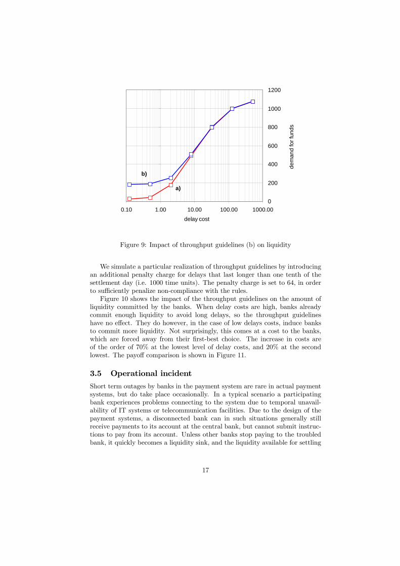
Figure 9: Impact of throughput guidelines (b) on liquidity

We simulate a particular realization of throughput guidelines by introducingan additional penalty charge for delays that last longer than one tenth of thesettlement day (i.e. 1000 time units). The penalty charge is set to 64, in orderto sufficiently penalize non-compliance with the rules.Figure 10 shows the impact of the throughput guidelines on the amount of

liquidity committed by the banks. When delay costs are high, banks alreadycommit enough liquidity to avoid long delays, so the throughput guidelineshave no effect. They do however, in the case of low delays costs, induce banksto commit more liquidity. Not surprisingly, this comes at a cost to the banks,which are forced away from their first-best choice. The increase in costs areof the order of 70% at the lowest level of delay costs, and 20% at the secondlowest. The payoff comparison is shown in Figure 11.

3.5 Operational incident

Short term outages by banks in the payment system are rare in actual paymentsystems, but do take place occasionally. In a typical scenario a participatingbank experiences problems connecting to the system due to temporal unavail-ability of IT systems or telecommunication facilities. Due to the design of thepayment systems, a disconnected bank can in such situations generally stillreceive payments to its account at the central bank, but cannot submit instruc-tions to pay from its account. Unless other banks stop paying to the troubledbank, it quickly becomes a liquidity sink, and the liquidity available for settling

17

a)

b)

-0.14

-0.12

-0.1

-0.08

-0.06

-0.04

-0.02

00.10 1.00 10.00 100.00 1000.00

delay cost

payo

ff

Figure 10: Impact of throughput guidelines (b) on payoffs

payments at other banks is reduced.19

In this set of simulations we ask the question of how much liquidity bankswould wish to commit in such a situation, i.e. what is the impact of an opera-tional outage on the demand for intraday credit. The banks are assumed to beunaware of the possible incident, and unable to discriminate among their coun-terparts, so the intraday liquidity management rule under Eq. 4 is still adopted.Under these assumptions, we simulated a scenario where a randomly selectedbank can receive, but cannot send payments for the first half of the settlementday. On average, this means that up to T/2N = 10.000/(2 · 15) ' 333 liquidityunits cannot be used by other banks as a source of liquidity20 . Depending onthe delay cost, this figure varies between 1900% and 30% of the average totalliquidity injected in the system at the beginning of the day (the first figure beingfor the case when both delay cost and liquidity demand are low, and the secondfor when costs liquidity demand are both high).We found that the effect of operational incidents on the demand for liquidity

is highest at a relative delay/liquidity cost ratio of 2 - hence fairly low in therange; at this point, the increase in intraday credit demand is 144 units, oran increase of 85%. It should be noted that banks do not compensate forthe full amount of liquidity "trapped" by the distressed bank, but prefer topartly make up for that, and partly increase delays. For higher delay costs,

19 see e.g. analysis on the impact of the 9/11 terrorist attacks in McAndrews and Potter(2002), Lacker (2004), and Soramäki et al (2007)20The shortage of liquidity equals the number of payment orders received by the distressed

bank, and not yet executed until the second half of the day.

18

a)

b)

0

200

400

600

800

1000

1200

0.1 1 10 100 1000cost ratio

dem

and

for f

unds

Figure 11: Liquidity - normal circumstances (a) and operational incidents (b)

delays remain approximately unchanged compared to the scenario without theincident. Finally, when delay costs are lower than liquidity costs (i.e. for a costratio <1), banks prefer to hold about the same amount of liquidity as withoutthe incident, and experience the delays caused by the reduced liquidity. Inthis case, the impact of an operational incident increases both the demand forliquidity (but less than what was trapped) and delays - more so the one whichis less costly.

4 Summary and conclusionsIn this paper we developed an agent-based, adaptive model of banks in a pay-ment system. Our main focus is on the demand for intraday credit under alterna-tive scenarios: i) a "benchmark" scenario, where payments flows are determinedby the initial liquidity, and by an exogenous arrival of payment instructions; ii)a system where, in addition, throughput guidelines are exogenously imposed iii)a system subject to operational incidents.It is well known that the demand for intraday credit is generated by a trade-

off between the costs associated with delaying payments, and liquidity costs.Simulating the model for different parameter values, we were able to draw withsome precision a liquidity demand function, which turns out to be is an S-shapedfunction of the delay / liquidity cost ratio. We also looked at the costs expe-rienced by the banks, as a function of the model’s parameters. By the processof individual payoff maximization, banks adjust their demand for liquidity up

19

a)

b)

0

200

400

600

800

1000

1200

1400

1600

1800

0.1 1 10 100 1000funds committed

dela

y pe

r pay

men

t

Figure 12: Delays as a function of cost ratio (b: incident)

(reducing delays) when delay costs increase, and down (increasing delays), whenthey rise. Interestingly however, the absolute delay cost remains approximatelyconstant when the ratio delay/liquidity costs changes. As expected, the de-mand for intraday credit is increased by an operational incident. However, thiseffect is found to be important only if liquidity is costly compared to delayingpayments. Likewise, throughput guidelines increase the demand for intradaycredit - as banks try to avoid penalties for not adhering to them. In total thisreduces the payoffs of the banks. Nevertheless, throughput guidelines may bebeneficial when additional benefits that are not in the current model are takeninto account (among these, benefits related to reducing operational risk).This model produces realistic behaviour, suggesting that it may be used to

investigate a wide array of issues in future applications. A number of extensionsare possible. First, alternative specifications for the instruction arrival processmay be applied (see e.g. Beyeler at al. (2006)). Alternatively, one could changethe assumptions on the banks’ network: while the complete network assumptionimplicitly adopted here fits well with e.g. the UK CHAPS system, an interestingquestion is how other topologies such as a scale free network topology such as inFedwire (Soramäki et al.. 2007) would affect the results. Also, different individ-ual preferences could be investigated. We assumed that banks are risk neutraland interested in maximising their immediate payoffs; it would be interestingto verify if the introduction of risk aversion and / or preferences over expectedstream of payoffs may change the results. Finally, more complex behaviour canbe easily studied within our model; for example, the "pay-as-much-as-you-can"rule for queuing payments could be replaced by sender limits. Similarly, more

20

sophisticated strategies can be easily modelled, supposing e.g. that banks keepconstant their actions for a number of periods (to gather more data and explorethe environment), instead of exploiting after a fixed amount of time what seemsto be the best action.

References[1] Angelini, P (1998), ‘’An Analysis of Competitive Externalities in Gross

Settlement Systems”, Journal of Banking and Finance n. 22, pages 1-18.

[2] Bank for International Settlements (2006), Statistics on payment andsettlement systems in selected countries - Figures for 2005 - Preliminaryversion. CPSS Publication No. 75.

[3] Barto, A G and Sutton, R S (1998), Reinforcement Learning: anintroduction. MIT Press, Cambridge, Massachusetts.

[4] Barto, A G, Sutton, R S and Brouwer, P S (1981), "Associativesearch network: A reinforcement learning associative memory". BiologicalCybernetics, 40, pages 201-211.

[5] Bech, M L and Soramäki, K (2002), "Liquidity, gridlocks and bankfailures in large value payment systems". in E-money and payment systemsReview, Central Banking Publications. London.

[6] Bech, M L and Garratt, R (2003), "The intraday liquidity managementgame", Journal of Economic Theory, vol. 109(2), pages 198-219.

[7] Bech, M L and Garratt, R (2006), "Illiquidity in the Interbank Pay-ment System Following Wide-Scale Disruptions". Federal Rererve Bank ofNew York Staff Report No. 239.

[8] Beyeler, W, Bech, M, Glass, R. and Soramäki K (2006), "Con-gestion and Cascades in Payment Systems". Federal Reserve Bank of NewYork Staff Report No. 259.

[9] Blume, L (1993), "The statistical mechanics of best-response strategyrevision". Games and Economic Behavior, 11, pages 111—145.

[10] Brown, G W (1951), "Iterative Solutions of Games by Fictitious Play"in Koopmans T C (Ed.), Activity Analysis of Production and Allocation,New York: Wiley.

[11] Buckle, S and Campbell, E (2003), "Settlement bank behaviour inreal-time gross settlement payment system". Bank of England Workingpaper No. 22.

[12] Devriese, J and Mitchell J (2006), "Liquidity Risk in Securities Set-tlement", Journal of Banking and Finance, v. 30, iss. 6, pages 1807-1834.

21

[13] Ellison, G (1993), "Learning, local interaction, and coordination",Econometrica, 61, pages 1047-1072.

[14] Foster, D P and Young H P (1998), "On the Nonconvergence of Fic-titious Play in Coordination Games", Games and Economic Behavior, v.25, iss. 1, pages 79-96.

[15] Fudenberg, D and Levine D K (1998), "The Theory of Learning inGames". MIT Press., Cambridge, Massachusetts.

[16] James, K and Willison M. (2004), "Collateral Posting Decisions inCHAPS Sterling", Bank of England Financial Stability Report, December2006.

[17] Kandori. M, Mailath, G J and Rob, R (1993), "Learning, Mutation,and Long Run Equilibria in Games", Econometrica, Vol. 61, No. 1. pages29-56.

[18] Krishna, V and Sjostrom, T (1995), "On the Convergence of FictitiousPlay", Mathematics of Operations Research 23(2), pages 479 - 511.

[19] Lacker, J M (2004), “Payment system disruptions and the federal reservefollowing September 11, 2001.” Journal of Monetary Economics, Vol. 51,No. 5, pages 935-965.

[20] McAndrews, J and Potter S M (2002), “The Liquidity Effects of theEvents of September 11, 2001”, FRBNY Economic Policy Review, Vol. 8,No. 2, pages 59-79.

[21] Soramäki, K, Bech, M L, Arnold, J, Glass R J and Beyeler, W E(2006), "The Topology of Interbank Payment Flows". Physica A Vol. 379,pages 317-333.

[22] Schlag, K (1995), "Why Imitate, and if so, How? A Boundedly RationalApproach to Multi-Armed Bandits", Journal of Economic Theory 78(1),pages 130—156.

[23] Watkins, C and Dayan P (1992), "Technical note: Q-learning", Ma-chine Learning, 8(3/4), pages 279-292.

[24] Willison, M (2005), "Real-Time Gross Settlement and hybrid paymentssystems: a comparison", Bank of England Working Paper No. 252.

[25] Young P (1993), "The evolution of conventions", Econometrica 61, pages57-84.

22