A comparison of methods to compute the ``effective duration'' of the autocorrelation function and an...

A comparison of methods to compute the “effective duration” ofthe autocorrelation function and an alternative proposal

Dario D’Orazio, Simona De Cesaris, and Massimo Garaia)

Department of Energetic, Nuclear and Environmental Control Engineering (DIENCA),University of Bologna, Viale Risorgimento, 2, 40136, Bologna, Italy

(Received 18 January 2011; revised 22 July 2011; accepted 22 July 2011)

The “effective duration” of the autocorrelation function (ACF), se, is an important factor in archi-

tectural and musical acoustics. For a general application, an accurate evaluation of se is relevant.

This paper is focused to the methods for the extraction of se values from the ACF. Various methods

have been proposed in literature for the extraction of the se from a given signal, but these methods

are not unambiguously defined or may not work properly in case of particular signals. Therefore,

the general use of these methods may sometimes give rise to questionable results. In the present

work, the methods existing in literature for extracting se are analyzed, their advantages and draw-

backs are summarized, and finally an alternative method is proposed. The proposed algorithm is

compared to those found in previous literature, applying them on the same sound signals (classic

literature references and other ones publicly available on the Internet). It is shown that the results

obtained with the proposed method are consistent with the results of the previous literature; more-

over the proposed method may overcome some of the limitations of the existing methods.VC 2011 Acoustical Society of America. [DOI: 10.1121/1.3624818]

PACS number(s): 43.55.Hy, 43.66.Mk, 43.66.Ba, 43.66.Lj [NX] Pages: 1954–1961

I. INTRODUCTION

The physiological model of perception based on the

autocorrelation function (ACF) has been first proposed by

Licklider,1 considering both time and frequency domains.

After this work, the model of monoaural perception based on

the autocorrelation function has been developed by several

authors. Cariani and Delgutte2 have shown the relation

between the shape of the autocorrelation histograms (all-order

interspike interval histograms for each channel) and the ACF.

The Licklider’s model has inspired many computational

auditory scene analyses.3–5 A complete review of the related

literature can be found in Refs. 6 and 7.

While the Licklider’s works has been focused on the

fine structure of the ACF and its relationship with pitch per-

ception, the correlation between the ACF envelope and the

subjective perception has been first calculated by Fourduiev8

to find the optimal reverberation time in relation to different

music pieces. Similarly to the definition of the “effective sig-

nal level and the “effective bandwidth” by Jeffress,9 Ando10

proposed a definition of the “effective duration” (se) of a

sound event related to the envelope decay of ACF. At first,

this quantity has been related to the subjective preference of

early reflections10–12 and then to the subjective preference of

the reverberation time.11,13

se and other factors extracted from ACF have been

widely used in different fields of acoustics. In architectural

acoustics, se is one of the independent variables of the nor-

mal factors related to the temporal perception.10–15 In musi-

cal acoustics, se is related to the analysis of performance.16

se has also been used to quantify the annoyance.17–20 In envi-

ronmental acoustics, se is used to analyze environmental

noise,17 soundscape quality, and aircraft noise.21,22

The envelope extraction has been performed using dif-

ferent methods, leading to different results even for the same

sound samples. Fourdouiev8 performed his envelope analysis

by using a tape correlator. In the following litera-

ture,10,11,13,16,23 the envelope analysis of ACF is numerical

and based on A-weighted signals. Three different algorithms

for the envelope extraction have been proposed by Ando

et al.24 for the extraction of se. The subjective plausibility of

the duration of the temporal window in the short time integra-

tion (2T) is a critical point of discussion. Ando discussed the

possibility to model the temporal integration of ACF on the

basis of a “psychological present.”25 Mouri et al.23 proposed

an optimal algorithm for the choice of the duration of the tem-

poral integration. Other kinds of analysis related to different

methods of integration have been presented by Kato et al.16

Others techniques of envelope extraction are treated in

the field of monaural detection. Rice26 using the statistical

analysis studied the envelope of narrow band Gaussian sig-

nals. Peterson et al.27 studied the performance of an ideal de-

tector of Gaussian noise and generalized the Rice’s statistics.

Marill,28 using a psychometric functions obtained in two al-

ternative forced choice,29 derived the probability density of

a detector. McGill30 showed that Marill’s results can be

derived from the statistics of an energy detector. Jeffress31

discussed the previous work basing on Zwislocki’s studies

on temporal integration.32 Urkowitz33 analyzed the detection

of deterministic signals in a rigorous mathematical form and

established sufficient conditions.

II. DEFINITIONS AND EXISTING DETECTION METHODS

In the field of room acoustics the ACF is usually defined

as16

a)Author to whom correspondence should be addressed. Electronic mail:

[email protected]

1954 J. Acoust. Soc. Am. 130 (4), October 2011 0001-4966/2011/130(4)/1954/8/$30.00 VC 2011 Acoustical Society of America

Au

tho

r's

com

plim

enta

ry c

op

y

Uðs; tÞ ¼ 1

2T

ðtþT

t�T

pðnÞpðnþ sÞdn (1)

where p(n) is the A-weighted sound pressure signal, 2T is

the width of the temporal window, and s is the time delay of

the ACF.

The normalized ACF has the form

/ðs; tÞ ¼ Uðs; tÞUð0; tÞ (2)

where U(0, t) can also be seen as the energy of the signal

inside the temporal window.

The “effective duration” of the ACF (se) is defined here,

following Ando,11 as “the first 10 percentile of envelope

decay of the normalized running ACF” expressed in decibels.

Many physiological models include an additive noise

term in the internal representation of a sound; this is equiva-

lent to take into account, in the analysis of correlation, a

threshold under which the decay is no more meaningful.

In the case of se, the first 10 dB of the decay are

assumed useful with a sufficient high signal to noise ratio,11

but only the first 5 dB of the decay are assumed linear and

the ACF envelope is only linearized over this range.

To compare the present work to the existing literature,16,23,24

a rectangular temporal window is chosen, with a width 2T¼ 2 s.

A. Peak detection method

In the so-called “peak detection method,” the ACF

peaks located over the threshold are linearly interpolated and

the abscissa of the �10 dB point on the interpolating straight

line estimates se.11

In the existing literature, it is not clear whether all peaks

should be taken into account or if only a subset of them is

meaningful for the envelope analysis.16,24 Some methods,

developed for pitch extraction from ACF,34,35 introduce a

selection of the “relevant peaks,” but these methods are ori-

ented to the selection of one single peak in the fine structure

analysis and are not focused on finding different peaks in an

envelope analysis. For the scope of the present work, the rel-

evant peaks are those contributing to the ACF envelope, but

in the existing literature, the selection criteria are not strictly

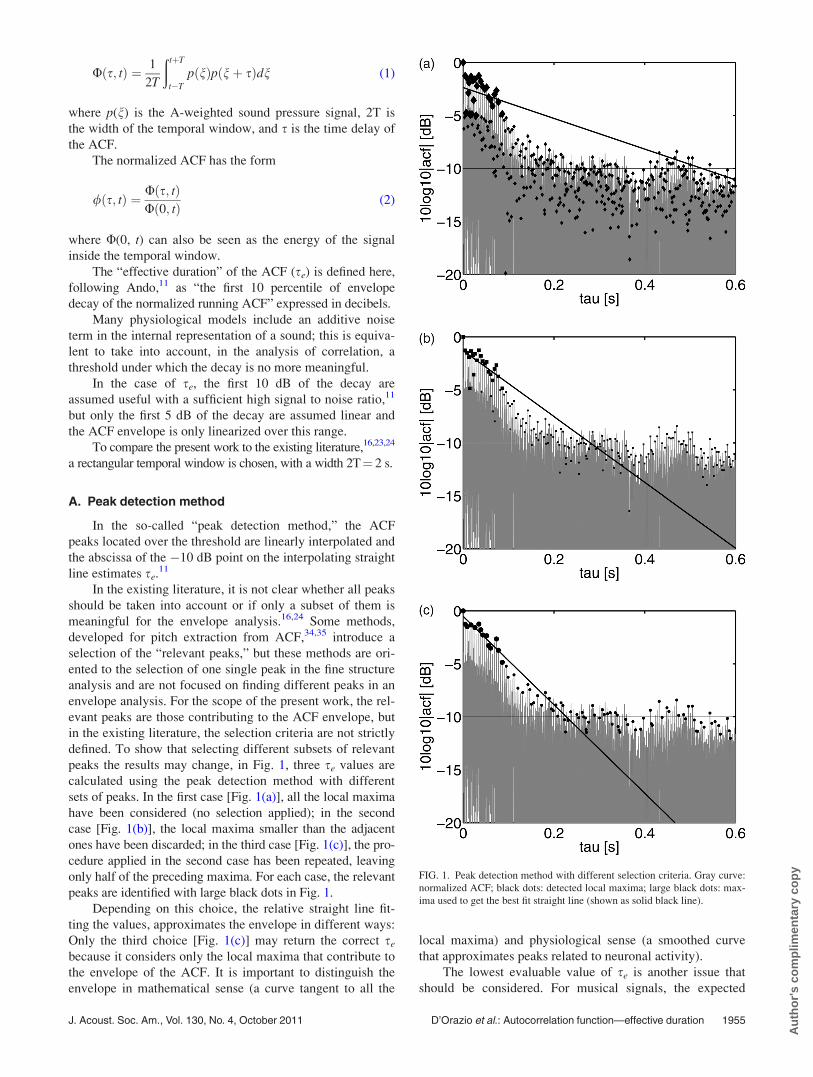
defined. To show that selecting different subsets of relevant

peaks the results may change, in Fig. 1, three se values are

calculated using the peak detection method with different

sets of peaks. In the first case [Fig. 1(a)], all the local maxima

have been considered (no selection applied); in the second

case [Fig. 1(b)], the local maxima smaller than the adjacent

ones have been discarded; in the third case [Fig. 1(c)], the pro-

cedure applied in the second case has been repeated, leaving

only half of the preceding maxima. For each case, the relevant

peaks are identified with large black dots in Fig. 1.

Depending on this choice, the relative straight line fit-

ting the values, approximates the envelope in different ways:

Only the third choice [Fig. 1(c)] may return the correct se

because it considers only the local maxima that contribute to

the envelope of the ACF. It is important to distinguish the

envelope in mathematical sense (a curve tangent to all the

local maxima) and physiological sense (a smoothed curve

that approximates peaks related to neuronal activity).

The lowest evaluable value of se is another issue that

should be considered. For musical signals, the expected

FIG. 1. Peak detection method with different selection criteria. Gray curve:

normalized ACF; black dots: detected local maxima; large black dots: max-

ima used to get the best fit straight line (shown as solid black line).

J. Acoust. Soc. Am., Vol. 130, No. 4, October 2011 D’Orazio et al.: Autocorrelation function—effective duration 1955

Au

tho

r's

com

plim

enta

ry c

op

y

values of se range from 10 to 200 ms (and more). For instru-

mental attacks or vocal glitches, the value of se can be 5 ms

or less.20 In these or analogous cases,19 the value of the first

relevant peak may be less than �5 dB, and thus the peak

detection method with a threshold of �5 dB may produce

meaningless results.

B. Backward integration method

A backward integration method, analogous to

Schroeder’s one,36 has ben proposed for the evaluation of

ACF envelope.16,24 The decay function D(t) can be obtained

as follows:

DðtÞ ¼ð0

t0

UðsÞj jds (3)

where t0> 0 is the initial time of the backward integration

and UðtÞ is the ACF.

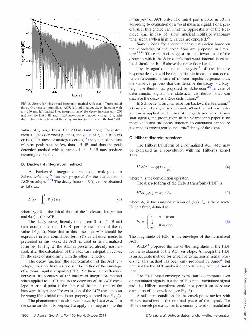
The decay curve, linearly fitted from 0 to �5 dB and

then extrapolated to �10 dB, permits extraction of the se

value (Fig. 2). Note that in this case, the ACF should be

expressed in non normalized form (U); in all other methods

presented in this work, the ACF is used in its normalized

form (/) (in Fig. 2, the ACF is presented already normal-

ized, after the calculation of the backward integration curve,

for the sake of uniformity with the other methods).

The decay function (the approximation of the ACF en-

velope) does not have a slope similar to that of the envelope

of a room impulse response (RIR). So there is a difference

between the accuracy of the backward integration method

when applied to a RIR and to the detection of the ACF enve-

lope. A critical point is the choice of the initial time of the

backward integration: The evaluation of the ACF envelope can

be wrong if this initial time is not properly selected (see Fig. 2).

The phenomenon has also been noted by Kato et al.16 In

the same article, it is proposed to apply the integration to the

initial part of ACF only: The initial part is fixed in 50 ms

according to evaluation of a vocal musical signal. For a gen-

eral use, this choice can limit the applicability of the tech-

nique, e.g., in case of “slow” musical motifs or stationary

tonal signals when high se values are expected.20

Some criteria for a correct decay estimation based on

the knowledge of the noise floor are proposed in litera-

ture.37,38 These methods suggest that the lower level of the

decay in which the Schroeder’s backward integral is calcu-

lated should be 10 dB above the noise floor level.

The Morgan’s statistical analysis39 of the impulse

response decay could be not applicable in case of autocorre-

lation functions. In case of a room impulse response, thus,

the statistical process that can describe the decay is a Ray-

leigh distribution, as proposed by Schroeder.40 In case of

deterministic signal, the statistical distribution that can

describe the decay is a Rice distribution.26

In Schroeder’s original paper on backward integration,36

a Gaussian like signal is supposed. When the backward inte-

gration is applied to deterministic signals instead of Gaus-

sian signals, the proof given in the Schroeder’s paper is no

more valid and the decay function so calculated cannot be

assumed as convergent to the “true” decay of the signal.

C. Hilbert discrete transform

The Hilbert transform of a normalized ACF /(s) may

be expressed as a convolution with the Hilbert’s kernel

1=ps:

H½/ðsÞ� ¼ /ðsÞ � 1

ps(4)

where * is the convolution operator.

The discrete form of the Hilbert transform (HDT) is

HDT /nf g ¼ /n � hn (5)

where /n is the sampled version of /(s); hn is the discrete

Hilbert filter, defined as

hn ¼0 n ¼ even

2

pnn ¼ odd:

8<: (6)

The magnitude of HDT is the envelope of the normalized

ACF.

Ando24 proposed the use of the magnitude of the HDT

for the evaluation of the ACF envelope. Although the HDT

is an accurate method for envelope extraction in signal proc-

essing, this method has been only proposed by Ando24 but

not used for the ACF analysis due to its heavy computational

load.

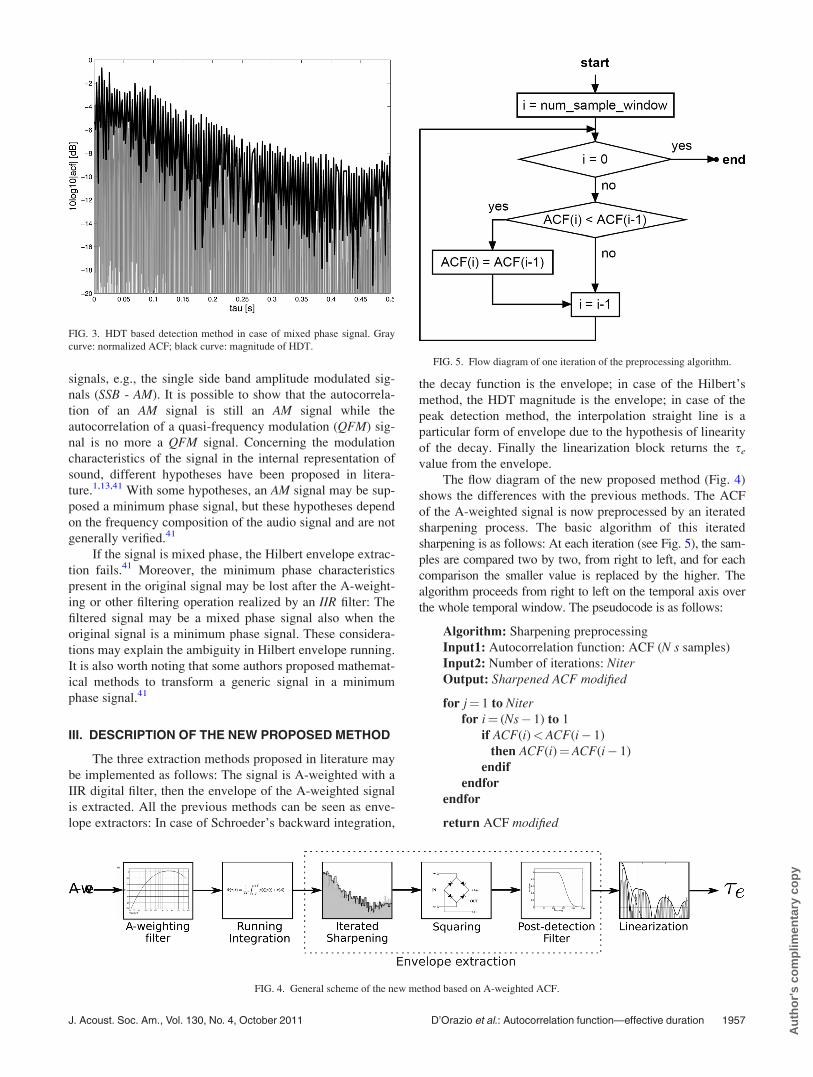
The HDT based envelope extraction is commonly used

on modulated signals, but the ACF is not a modulated signal

and the Hilbert transform could not permit an adequate

extraction of the envelope (see Fig. 3).

A sufficient condition for the envelope extraction with

Hilbert transform is the minimal phase of the signal. The

Hilbert envelope extraction is commonly used on modulated

FIG. 2. Schroeder’s backward integration method with two different initial

times. Gray curve: normalized ACF; left solid curve: decay function with

t0¼ 250 ms; left dashed line: interpolation of the decay function (t0¼ 250

ms) over the first 5 dB; right solid curve: decay function with t0¼ 2 s; right

dashed line: interpolation of the decay function (t0¼ 2 s) over the first 5 dB.

1956 J. Acoust. Soc. Am., Vol. 130, No. 4, October 2011 D’Orazio et al.: Autocorrelation function—effective duration

Au

tho

r's

com

plim

enta

ry c

op

y

signals, e.g., the single side band amplitude modulated sig-

nals (SSB - AM). It is possible to show that the autocorrela-

tion of an AM signal is still an AM signal while the

autocorrelation of a quasi-frequency modulation (QFM) sig-

nal is no more a QFM signal. Concerning the modulation

characteristics of the signal in the internal representation of

sound, different hypotheses have been proposed in litera-

ture.1,13,41 With some hypotheses, an AM signal may be sup-

posed a minimum phase signal, but these hypotheses depend

on the frequency composition of the audio signal and are not

generally verified.41

If the signal is mixed phase, the Hilbert envelope extrac-

tion fails.41 Moreover, the minimum phase characteristics

present in the original signal may be lost after the A-weight-

ing or other filtering operation realized by an IIR filter: The

filtered signal may be a mixed phase signal also when the

original signal is a minimum phase signal. These considera-

tions may explain the ambiguity in Hilbert envelope running.

It is also worth noting that some authors proposed mathemat-

ical methods to transform a generic signal in a minimum

phase signal.41

III. DESCRIPTION OF THE NEW PROPOSED METHOD

The three extraction methods proposed in literature may

be implemented as follows: The signal is A-weighted with a

IIR digital filter, then the envelope of the A-weighted signal

is extracted. All the previous methods can be seen as enve-

lope extractors: In case of Schroeder’s backward integration,

the decay function is the envelope; in case of the Hilbert’s

method, the HDT magnitude is the envelope; in case of the

peak detection method, the interpolation straight line is a

particular form of envelope due to the hypothesis of linearity

of the decay. Finally the linearization block returns the se

value from the envelope.

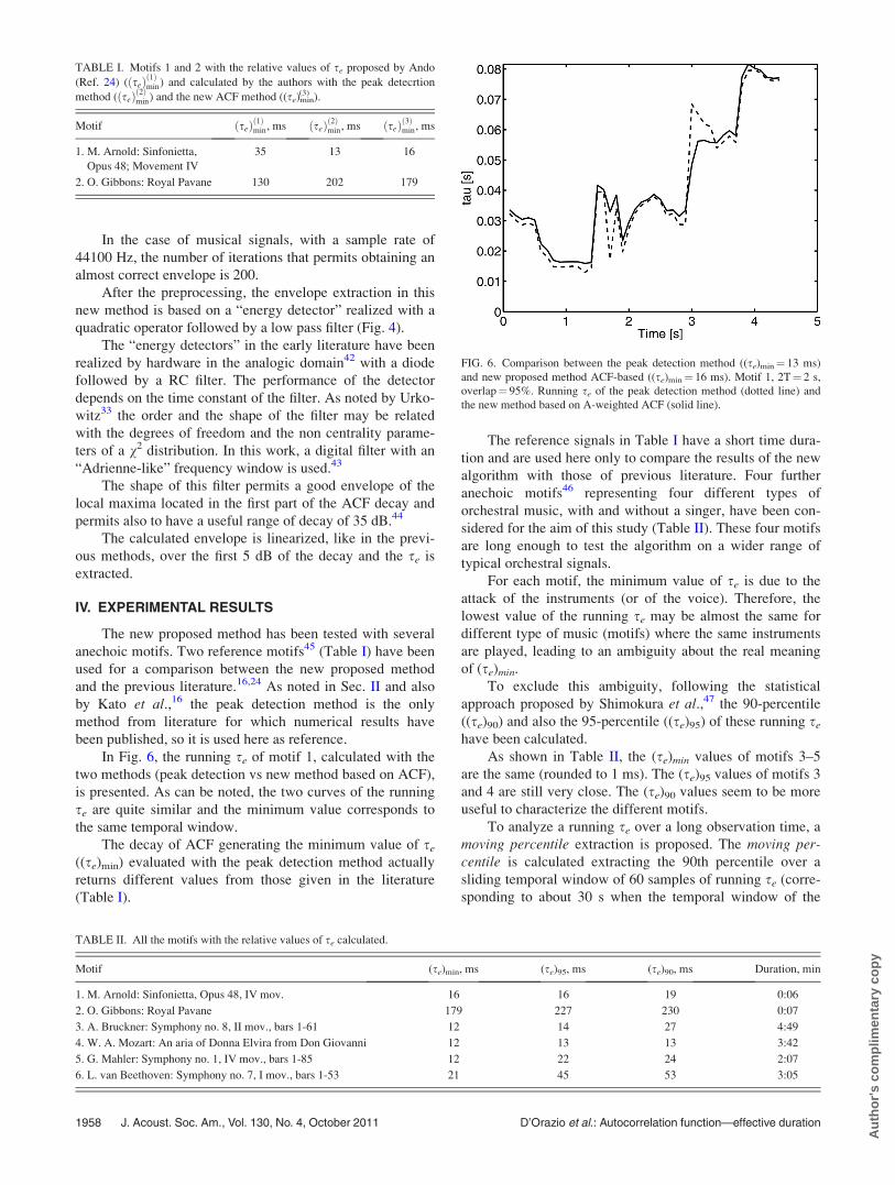
The flow diagram of the new proposed method (Fig. 4)

shows the differences with the previous methods. The ACF

of the A-weighted signal is now preprocessed by an iterated

sharpening process. The basic algorithm of this iterated

sharpening is as follows: At each iteration (see Fig. 5), the sam-

ples are compared two by two, from right to left, and for each

comparison the smaller value is replaced by the higher. The

algorithm proceeds from right to left on the temporal axis over

the whole temporal window. The pseudocode is as follows:

Algorithm: Sharpening preprocessing

Input1: Autocorrelation function: ACF (N s samples)

Input2: Number of iterations: NiterOutput: Sharpened ACF modified

for j¼ 1 to Niterfor i¼ (Ns� 1) to 1

if ACF(i)<ACF(i� 1)

then ACF(i)¼ACF(i� 1)

endif

endfor

endfor

return ACF modified

FIG. 3. HDT based detection method in case of mixed phase signal. Gray

curve: normalized ACF; black curve: magnitude of HDT.

FIG. 4. General scheme of the new method based on A-weighted ACF.

FIG. 5. Flow diagram of one iteration of the preprocessing algorithm.


Au

tho

r's

com

plim

enta

ry c

op

y

In the case of musical signals, with a sample rate of

44100 Hz, the number of iterations that permits obtaining an

almost correct envelope is 200.

After the preprocessing, the envelope extraction in this

new method is based on a “energy detector” realized with a

quadratic operator followed by a low pass filter (Fig. 4).

The “energy detectors” in the early literature have been

realized by hardware in the analogic domain42 with a diode

followed by a RC filter. The performance of the detector

depends on the time constant of the filter. As noted by Urko-

witz33 the order and the shape of the filter may be related

with the degrees of freedom and the non centrality parame-

ters of a v2 distribution. In this work, a digital filter with an

“Adrienne-like” frequency window is used.43

The shape of this filter permits a good envelope of the

local maxima located in the first part of the ACF decay and

permits also to have a useful range of decay of 35 dB.44

The calculated envelope is linearized, like in the previ-

ous methods, over the first 5 dB of the decay and the se is

extracted.

IV. EXPERIMENTAL RESULTS

The new proposed method has been tested with several

anechoic motifs. Two reference motifs45 (Table I) have been

used for a comparison between the new proposed method

and the previous literature.16,24 As noted in Sec. II and also

by Kato et al.,16 the peak detection method is the only

method from literature for which numerical results have

been published, so it is used here as reference.

In Fig. 6, the running se of motif 1, calculated with the

two methods (peak detection vs new method based on ACF),

is presented. As can be noted, the two curves of the running

se are quite similar and the minimum value corresponds to

the same temporal window.

The decay of ACF generating the minimum value of se

((se)min) evaluated with the peak detection method actually

returns different values from those given in the literature

(Table I).

The reference signals in Table I have a short time dura-

tion and are used here only to compare the results of the new

algorithm with those of previous literature. Four further

anechoic motifs46 representing four different types of

orchestral music, with and without a singer, have been con-

sidered for the aim of this study (Table II). These four motifs

are long enough to test the algorithm on a wider range of

typical orchestral signals.

For each motif, the minimum value of se is due to the

attack of the instruments (or of the voice). Therefore, the

lowest value of the running se may be almost the same for

different type of music (motifs) where the same instruments

are played, leading to an ambiguity about the real meaning

of (se)min.

To exclude this ambiguity, following the statistical

approach proposed by Shimokura et al.,47 the 90-percentile

((se)90) and also the 95-percentile ((se)95) of these running se

have been calculated.

As shown in Table II, the (se)min values of motifs 3–5

are the same (rounded to 1 ms). The (se)95 values of motifs 3

and 4 are still very close. The (se)90 values seem to be more

useful to characterize the different motifs.

To analyze a running se over a long observation time, a

moving percentile extraction is proposed. The moving per-centile is calculated extracting the 90th percentile over a

sliding temporal window of 60 samples of running se (corre-

sponding to about 30 s when the temporal window of the

TABLE I. Motifs 1 and 2 with the relative values of se proposed by Ando

(Ref. 24) ( seð Þð1Þmin) and calculated by the authors with the peak detecrtion

method ( seð Þð2Þmin) and the new ACF method ((se)min(3) ).

Motif seð Þð1Þmin, ms seð Þð2Þmin, ms seð Þð3Þmin, ms

1. M. Arnold: Sinfonietta,

Opus 48; Movement IV

35 13 16

2. O. Gibbons: Royal Pavane 130 202 179

FIG. 6. Comparison between the peak detection method ((se)min¼ 13 ms)

and new proposed method ACF-based ((se)min¼ 16 ms). Motif 1, 2T¼ 2 s,

overlap¼ 95%. Running se of the peak detection method (dotted line) and

the new method based on A-weighted ACF (solid line).

TABLE II. All the motifs with the relative values of se calculated.

Motif (se)min, ms (se)95, ms (se)90, ms Duration, min

1. M. Arnold: Sinfonietta, Opus 48, IV mov. 16 16 19 0:06

2. O. Gibbons: Royal Pavane 179 227 230 0:07

3. A. Bruckner: Symphony no. 8, II mov., bars 1-61 12 14 27 4:49

4. W. A. Mozart: An aria of Donna Elvira from Don Giovanni 12 13 13 3:42

5. G. Mahler: Symphony no. 1, IV mov., bars 1-85 12 22 24 2:07

6. L. van Beethoven: Symphony no. 7, I mov., bars 1-53 21 45 53 3:05


Au

tho

r's

com

plim

enta

ry c

op

y

running se is set at 2T¼ 2 s with an overlap of 75%) with a

shift of 15 samples for each step.

Motifs 3–6 are long enough to permit the computation

of a running integration of the percentile values of se using a

large time window. The running integration gives a smooth

curve, indicating the overall trend of (se)min (Figs. 7 and 8).

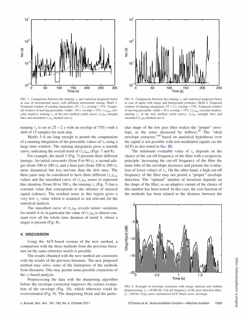
For example, the motif 3 (Fig. 7) presents three different

timings: An initial crescendo (from 0 to 90 s), a second ada-

gio (from 100 to 200 s), and a final part (from 200 to 300 s),

more dynamical but less nervous than the first ones. The

three parts may be considered to have three different (se)min

values and the smoothed curve of (se)90 seems to represent

this situation. From 90 to 100 s, the running se (Fig. 7) has a

constant value that corresponds to the absence of musical

signal (silence). The residual noise in this region gives a

very low se value which is assumed as not relevant for the

statistical analysis.

The smoothed curve of (se)90 reveals minor variations

for motifs 4–6; in particular the value of (se)90 is almost con-

stant over all the whole time duration of motif 4, where a

singer is present (Fig. 8).

V. DISCUSSION

Using the ACF-based version of the new method, a

comparison with the three methods from the previous litera-

ture on the same reference motifs is possible.

The results obtained with the new method are consistent

with the results of the previous literature. The new proposed

method may solve some of the limitations of the methods

from literature: This may permit some possible extensions of

the se-based analysis.

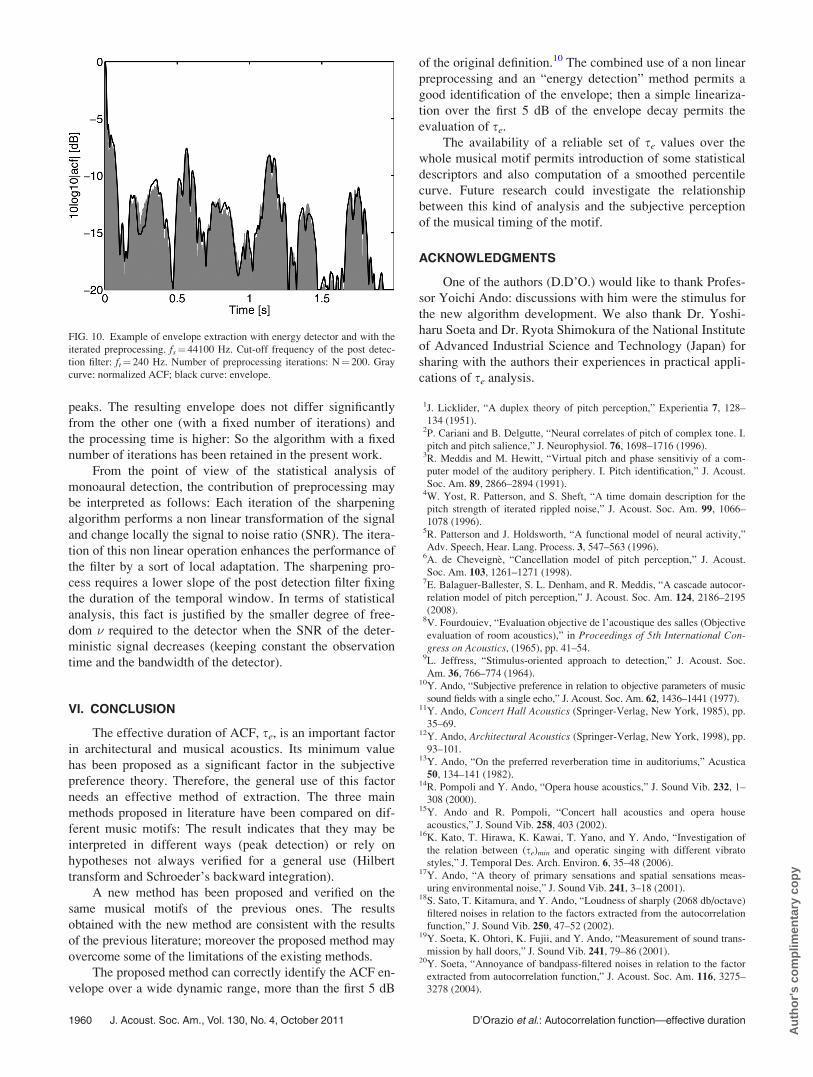
Preprocessing the data with the sharpening algorithm

before the envelope extraction improves the correct evalua-

tion of the envelope (Fig. 10), which otherwise could be

overestimated (Fig. 9). The sharpening block and the partic-

ular shape of the low pass filter realize the “proper” enve-

lope, in the sense discussed by Jeffress.42 The “ideal

envelope extractor,”48 based on analytical hypotheses over

the signal is not possible with non modulated signals (as the

ACF) as also noted in Sec. III.

The minimum evaluable value of se depends on the

choice of the cut-off frequency of the filter with a reciprocity

principle: Increasing the cut-off frequency of the filter the

main lobe of the envelope decreases and permits the evalua-

tion of lower values of se. On the other hand, a high cut-off

frequency of the filter may not permit a “proper” envelope

detection. The “optimal” number of iterations depends on

the shape of the filter, so an adaptive variant of the choice of

this number has been tested: In this case, the cost function of

the methods has been related to the distance between the

FIG. 7. Comparison between the running se and statistical proposed factor

in case of instrumental music with different metronomic timing. Motif 3.

Temporal window of running integration: 2T¼ 2 s, overlap¼ 75%. Tempo-

ral window of moving percentile: width¼ 30 s, overlap¼ 75%. (se)min (cir-

cular marker), running se of the new method (solid curve), (se)90 (straight

line) and smoothed (se)90 (dashed curve).

FIG. 8. Comparison between the running se and statistical proposed factor

in case of opera with singer and background orchestra. Motif 4. Temporal

window of running integration: 2T¼ 2 s, overlap¼ 75%. Temporal window

of moving percentile: width¼ 30 s, overlap¼ 75%. (se)min (circular marker),

running se of the new method (solid curve), (se)90 (straight line) and

smoothed (se)90 (dashed curve).

FIG. 9. Example of envelope extraction with energy detector and without

preprocessing. fs¼ 44100 Hz. Cut-off frequency of the post detection filter:

ft¼ 240 Hz. Gray curve: normalized ACF; black curve: envelope.


Au

tho

r's

com

plim

enta

ry c

op

y

peaks. The resulting envelope does not differ significantly

from the other one (with a fixed number of iterations) and

the processing time is higher: So the algorithm with a fixed

number of iterations has been retained in the present work.

From the point of view of the statistical analysis of

monoaural detection, the contribution of preprocessing may

be interpreted as follows: Each iteration of the sharpening

algorithm performs a non linear transformation of the signal

and change locally the signal to noise ratio (SNR). The itera-

tion of this non linear operation enhances the performance of

the filter by a sort of local adaptation. The sharpening pro-

cess requires a lower slope of the post detection filter fixing

the duration of the temporal window. In terms of statistical

analysis, this fact is justified by the smaller degree of free-

dom � required to the detector when the SNR of the deter-

ministic signal decreases (keeping constant the observation

time and the bandwidth of the detector).

VI. CONCLUSION

The effective duration of ACF, se, is an important factor

in architectural and musical acoustics. Its minimum value

has been proposed as a significant factor in the subjective

preference theory. Therefore, the general use of this factor

needs an effective method of extraction. The three main

methods proposed in literature have been compared on dif-

ferent music motifs: The result indicates that they may be

interpreted in different ways (peak detection) or rely on

hypotheses not always verified for a general use (Hilbert

transform and Schroeder’s backward integration).

A new method has been proposed and verified on the

same musical motifs of the previous ones. The results

obtained with the new method are consistent with the results

of the previous literature; moreover the proposed method may

overcome some of the limitations of the existing methods.

The proposed method can correctly identify the ACF en-

velope over a wide dynamic range, more than the first 5 dB

of the original definition.10 The combined use of a non linear

preprocessing and an “energy detection” method permits a

good identification of the envelope; then a simple lineariza-

tion over the first 5 dB of the envelope decay permits the

evaluation of se.

The availability of a reliable set of se values over the

whole musical motif permits introduction of some statistical

descriptors and also computation of a smoothed percentile

curve. Future research could investigate the relationship

between this kind of analysis and the subjective perception

of the musical timing of the motif.

ACKNOWLEDGMENTS

One of the authors (D.D’O.) would like to thank Profes-

sor Yoichi Ando: discussions with him were the stimulus for

the new algorithm development. We also thank Dr. Yoshi-

haru Soeta and Dr. Ryota Shimokura of the National Institute

of Advanced Industrial Science and Technology (Japan) for

sharing with the authors their experiences in practical appli-

cations of se analysis.

1J. Licklider, “A duplex theory of pitch perception,” Experientia 7, 128–

134 (1951).2P. Cariani and B. Delgutte, “Neural correlates of pitch of complex tone. I.

pitch and pitch salience,” J. Neurophysiol. 76, 1698–1716 (1996).3R. Meddis and M. Hewitt, “Virtual pitch and phase sensitiviy of a com-

puter model of the auditory periphery. I. Pitch identification,” J. Acoust.

Soc. Am. 89, 2866–2894 (1991).4W. Yost, R. Patterson, and S. Sheft, “A time domain description for the

pitch strength of iterated rippled noise,” J. Acoust. Soc. Am. 99, 1066–

1078 (1996).5R. Patterson and J. Holdsworth, “A functional model of neural activity,”

Adv. Speech, Hear. Lang. Process. 3, 547–563 (1996).6A. de Cheveigne, “Cancellation model of pitch perception,” J. Acoust.

Soc. Am. 103, 1261–1271 (1998).7E. Balaguer-Ballester, S. L. Denham, and R. Meddis, “A cascade autocor-

relation model of pitch perception,” J. Acoust. Soc. Am. 124, 2186–2195

(2008).8V. Fourdouiev, “Evaluation objective de l’acoustique des salles (Objective

evaluation of room acoustics),” in Proceedings of 5th International Con-gress on Acoustics, (1965), pp. 41–54.

9L. Jeffress, “Stimulus-oriented approach to detection,” J. Acoust. Soc.

Am. 36, 766–774 (1964).10Y. Ando, “Subjective preference in relation to objective parameters of music

sound fields with a single echo,” J. Acoust. Soc. Am. 62, 1436–1441 (1977).11Y. Ando, Concert Hall Acoustics (Springer-Verlag, New York, 1985), pp.

35–69.12Y. Ando, Architectural Acoustics (Springer-Verlag, New York, 1998), pp.

93–101.13Y. Ando, “On the preferred reverberation time in auditoriums,” Acustica

50, 134–141 (1982).14R. Pompoli and Y. Ando, “Opera house acoustics,” J. Sound Vib. 232, 1–

308 (2000).15Y. Ando and R. Pompoli, “Concert hall acoustics and opera house

acoustics,” J. Sound Vib. 258, 403 (2002).16K. Kato, T. Hirawa, K. Kawai, T. Yano, and Y. Ando, “Investigation of

the relation between (se)min and operatic singing with different vibrato

styles,” J. Temporal Des. Arch. Environ. 6, 35–48 (2006).17Y. Ando, “A theory of primary sensations and spatial sensations meas-

uring environmental noise,” J. Sound Vib. 241, 3–18 (2001).18S. Sato, T. Kitamura, and Y. Ando, “Loudness of sharply (2068 db/octave)

filtered noises in relation to the factors extracted from the autocorrelation

function,” J. Sound Vib. 250, 47–52 (2002).19Y. Soeta, K. Ohtori, K. Fujii, and Y. Ando, “Measurement of sound trans-

mission by hall doors,” J. Sound Vib. 241, 79–86 (2001).20Y. Soeta, “Annoyance of bandpass-filtered noises in relation to the factor

extracted from autocorrelation function,” J. Acoust. Soc. Am. 116, 3275–

3278 (2004).

FIG. 10. Example of envelope extraction with energy detector and with the

iterated preprocessing. fs¼ 44100 Hz. Cut-off frequency of the post detec-

tion filter: ft¼ 240 Hz. Number of preprocessing iterations: N¼ 200. Gray

curve: normalized ACF; black curve: envelope.


Au

tho

r's

com

plim

enta

ry c

op

y

21K. Fujii, Y. Soeta, and Y. Ando, “Acoustical properties of aircraft noise meas-

ured by temporal and spatial factors,” J. Sound Vib. 241, 69–78 (2001).22H. Sakai, S. Sato, N. Prodi, and R. Pompoli, “Measurement of regional

environmental noise by use of a pc-based system. an application to the noise

near airport ‘G. Marconi’ in Bologna,” J. Sound Vib. 241, 57–68 (2001).23K. Mouri and K. Akiyama, “Preliminary study on raccomended time dura-

tion of source signals to be analyzed, in relation to its effective duration of

the auto-correlation function,” J. Sound Vib. 241, 87–95 (2001).24Y. Ando, T. Okano, and Y. Takezoe, “The running autocorrelation func-

tion of different music signals relating to preferred temporal parameters of

sound fields,” J. Acoust. Soc. Am. 86, 644–649 (1989).25P. Fraisse, “Rhythm and tempo,” in The Psychology of Music (Academic,

New York, 1982), pp. 149–180.26S. O. Rice, “Mathematical analysis of random noise,” Bell Systems Tech.

J. 24, 46–156 (1954).27W. W. Peterson, T.G. Birdsall, and W.C. Fox, “The theory of signal

detectability” IEEE Trans. Inform. Theory 4, 172–212 (1954).28T. Marill, “Detection theory and psychophysics,” Tech. Report No. 142

319, Research Laboratory of Electronics, MA Institute of Technology

(1956), pp. 1–73.29L. L. Thurstone, “A law of comparative judgment,” Psychol. Rev. 34,

273–286 (1927).30W. J. McGill, “Variations on Marrill’s detection formula,” J. Acoust. Soc.

Am. 43, 70–73 (1968).31L. Jeffress, “Stimulus-oriented approach to detection reexamined,”

J. Acoust. Soc. Am. 41, 480–488 (1967).32J. Zwislocki, “Theory of temporal auditory summation,” J. Acoust. Soc.

Am. 32, 1046–1060 (1960).33H. Urkowitz, “Energy detection of unknown deterministic signals,” Proc.

IEEE 55, 523–531 (1967).34C. Shahnaz, W. Zhu, and M. Ahmad, “A robust pitch estimation approach

for colored noise-corrupted speech,” IEEE Int. Symp. Circuits Syst. 4,

3143–3146 (2005).35J. Brown and M. Puckette, “Calculation of a ‘narrowed’ autocorrelation

function,” J. Acoust. Soc. Am. 85, 1595–1601 (1989).

36M. Schroeder, “New method of measuring reverberation time,” J. Acoust.

Soc. Am. 37, 407–412 (1965).37R. Kurer and U. Kurze, “Integration method of reverberating evaluation

(Integrationsver- fahren zur nachhallauswertung),” Acustica 19, 314–322

(1967).38M. Vorlander and H. Bietz, “Comparison of methods for measuring rever-

beration time” Acustica 80, 205215 (1994).39D. Morgan, “A parametric error analysis of the backward integration

method for reverberation time estimation,” J. Acoust. Soc. Am. 101,

2686–2693 (1997).40M. Schroeder, “Statistical parameters of the frequency response curves of

large rooms,” J. Audio Eng. Soc. 35, 299–306 (1987).41R. Kumaresan, and A. Rao, “Model-based approach to envelope and posi-

tive instantaneous frequency estimation of signals with speech

applications,” J. Acoust. Soc. Am. 105, 1912–1924 (1999).42L. Jeffress, “Mathematical and electrical models of auditory detection,” J.

Acoust. Soc. Am. 44, 187–203 (1968).43M. Garai and P. Guidorzi, “European methodology for testing the airborne

sound insulation characteristics of noise barriers in situ: Experimental ver-

ification and comparison with laboratory data,” J. Acoust. Soc. Am. 108,

1054–1067 (2000).44F. Harris, “On the use of windows for harmonic analysis with the discrete

fourier transform,” Proc. IEEE 66, 51–83 (1978).45A. Burd, “Nachfaller musik fur akustische modelluntersuchungen

(Anechoic music for research on acoustic models),” Rundfunktechn. Mitt.

13, 200–201 (1969).46J. Patven, V. Pulkki, and T. Lokki, “Anechoic recording system for sym-

phony orchestra,” Acta Acust. Acust. 94, 856–865 (2008).47R. Shimokura, A. Cocchi, L. Tronchin, and M. C. Consumi “Calculation

of IACC of any musical signal convolved with impulse response by using

the interaural cross-correlation function of the sound field and the autocor-

relation function of the sound source,” J. South China Univ. Technol.,

Nat. Sci. 35, 88–91 (2007).48J. Goldstein, “Auditory spectral filtering and monoaural phase perception,”

J. Acoust. Soc. Am. 41, 458–479 (1966).


Au

tho

r's

com

plim

enta

ry c

op

y

A comparison of methods to compute the ``effective duration'' of the autocorrelation function and an...

Documents

Transcript of A comparison of methods to compute the ``effective duration'' of the autocorrelation function and an...