A comparison of eight metamodeling techniques for the simulation of N 2 O fluxes and N leaching from...

This article appeared in a journal published by Elsevier. The attachedcopy is furnished to the author for internal non-commercial researchand education use, including for instruction at the authors institution

and sharing with colleagues.

Other uses, including reproduction and distribution, or selling orlicensing copies, or posting to personal, institutional or third party

websites are prohibited.

In most cases authors are permitted to post their version of thearticle (e.g. in Word or Tex form) to their personal website orinstitutional repository. Authors requiring further information

regarding Elsevier’s archiving and manuscript policies areencouraged to visit:

http://www.elsevier.com/copyright

http://www.elsevier.com/copyright

Author's personal copy

A comparison of eight metamodeling techniques for the simulation of N2O fluxesand N leaching from corn crops

Nathalie Villa-Vialaneix a,b,*, Marco Follador c, Marco Ratto d, Adrian Leip c

a IUT de Perpignan (Dpt STID, Carcassonne), Univ. Perpignan, Via Domitia, Franceb Institut de Mathématiques de Toulouse, Université de Toulouse, Francec European Commission, Institute for Environment and Sustainability, CCU, Ispra, Italyd European Commission, Econometrics and Applied Statistics Unit, Ispra, Italy

a r t i c l e i n f o

Article history:Received 18 October 2010Received in revised form15 April 2011Accepted 1 May 2011Available online 8 June 2011

Keywords:MetamodelingSplinesSVMNeural networkRandom forestN2O fluxN leachingAgriculture

a b s t r a c t

The environmental costs of intensive farming activities are often under-estimated or not traded by themarket, even though they play an important role in addressing future society’s needs. The estimation ofnitrogen (N) dynamics is thus an important issue which demands detailed simulation based methodsand their integrated use to correctly represent complex and non-linear interactions into croppingsystems. To calculate the N2O flux and N leaching from European arable lands, a modeling framework hasbeen developed by linking the CAPRI agro-economic dataset with the DNDC-EUROPE bio-geo-chemicalmodel. But, despite the great power of modern calculators, their use at continental scale is often toocomputationally costly. By comparing several statistical methods this paper aims to design a metamodelable to approximate the expensive code of the detailed modeling approach, devising the best compro-mise between estimation performance and simulation speed. We describe the use of two parametric(linear) models and six non-parametric approaches: two methods based on splines (ACOSSO and SDR),one method based on kriging (DACE), a neural networks method (multilayer perceptron, MLP), SVM anda bagging method (random forest, RF). This analysis shows that, as long as few data are available to trainthe model, splines approaches lead to best results, while when the size of training dataset increases, SVMand RF provide faster and more accurate solutions.

� 2011 Elsevier Ltd. All rights reserved.

1. Introduction

The impact of modern agriculture on the environment is welldocumented (Power, 2010; Tilman et al., 2002; Scherr and Sthapit,2009; FAO, 2007, 2005; Singh, 2000; Matson et al., 1997). Intensivefarming has a high consumption of nitrogen, which is often in-efficiently used, particularly in livestock production systems (Leipet al., in press a; Webb et al., 2005; Oenema et al., 2007;Chadwick, 2005). This leads to a large surplus of nitrogen whichis lost to the environment. Up to 95% of ammonia emission inEurope have their origin in agricultural activities (Kirchmann et al.,1998; Leip et al., 2011) contributing to eutrophication, loss ofbiodiversity and health problems. Beside NH3, nitrate leachingbelow the soil root zone and entering the groundwater posesa particular problem for the quality of drinking water (van Grinsven

et al., 2006). Additionally, agricultural sector is the major source ofanthropogenic emissions of N2O from the soils, mainly as a conse-quence of the application of mineral fertilizer or manure nitrogen(Del Grosso et al., 2006; Leip et al., in press b, 2005; EuropeanEnvironment Agency, 2010). N2O is a potent greenhouse gas(GHG) contributing with each kilogram emitted about 300 timesmore to global warming than the same mass emitted as CO2, on thebasis of a 100-years time horizon (Intergovernmental Panel onClimate Change, 2007).

Various European legislations attempt to reduce the environ-mental impact of the agriculture sector, particularly the NitratesDirective (European Council, 1991) and the Water FrameworkDirective (European Council, 2000). Initially, however, complianceto these directives was poor (Oenema et al., 2009; EuropeanCommission, 2002). Therefore, with the last reform of theCommon Agricultural Policy (CAP) in the year 2003 (EuropeanCouncil, 2003), the European Union introduced a compulsoryCross-Compliance (CC) mechanism to improve compliance with 18environmental, food safety, animal welfare, and animal and planthealth standards (Statutory Management Requirements, SMRs) aswell as with requirements to maintain farmlands in good

* Corresponding author. Institut de Mathématiques de Toulouse, Université PaulSabatier, 118 route de Narbonne, F-31062 Toulouse cedex 9, France. Tel.: þ33 5 61 5563 58.

E-mail address: [email protected] (N. Villa-Vialaneix).

Contents lists available at ScienceDirect

Environmental Modelling & Software

journal homepage: www.elsevier .com/locate/envsoft

1364-8152/$ e see front matter � 2011 Elsevier Ltd. All rights reserved.doi:10.1016/j.envsoft.2011.05.003

Environmental Modelling & Software 34 (2012) 51e66


agricultural and environmental condition (Good Agricultural andEnvironment Condition requirements, GAECs), as prerequisite forreceiving direct payments (European Union Commission, 2004,2009; European Council, 2009; Dimopoulus et al., 2007;Jongeneel et al., 2007). The SMRs are based on pre-existing EUDirectives and Regulations such as Nitrate Directives. The GAECsfocus on soil erosion, soil organic matter, soil structure anda minimum level of maintenance; for each of these issues a numberof standards are listed (Alliance Environnement, 2007).

It remains nevertheless a challenge to monitor compliance andto assess the impact of the cross-compliance legislations not onlyon the environment, but also on animal welfare, farmer’s income,production levels, etc. In order to help with this task, the EU-projectCross-Compliance Assessment Tool (CCAT) developed a simulationplatform to provide scientifically sound and regionally differenti-ated responses to various farming scenarios (Elbersen et al., 2010;Jongeneel et al., 2007).

CCAT integrates complementary models to assess changes inorganic carbon and nitrogen fluxes from soils (De Vries et al., 2008).Carbon and nitrogen turnover are very complex processes, char-acterized by a high spatial variability and a strong dependence onenvironmental factors such as meteorological conditions and soils(Shaffer and Ma, 2001; Zhang et al., 2002). Quantification of fluxes,and specifically a meaningful quantification of the response tomitigation measures at the regional level requires the simulation offarmmanagement and the soil/plant/atmosphere continuum at thehighest possible resolution (Anderson et al., 2003; Leip et al., inpress b). For the simulation of N2O fluxes and N leaching, theprocess-based biogeochemistry model DNDC-EUROPE (Leip et al.,2008; Li et al., 1992; Li, 2000) was used. As DNDC-EUROPE isa complex model imposing high computational costs, the timeneeded to obtain simulation results in large-scale applications(such as the European scale) can be restrictive. In particular, thedirect use of the deterministic model is prohibited to extract effi-ciently estimations of the evolution of N2O fluxes and N leachingunder changing conditions. Hence, there is a need for a second levelof abstraction, modeling the DNDC-EUROPE model itself, which iscalled a metamodel (see Section 2 for a more specific definition ofthe concept of metamodeling). Metamodels are defined froma limited number of deterministic simulations for specific appli-cations and/or scenario and allow to obtain fast estimations.

This issue is a topic of high interest that has previously beentackled in several papers: among others, Bouzaher et al. (1993)develop a parametric model, including spatial dependency, tomodel water pollution. Krysanova and Haberlandt (2002) andHaberlandt et al. (2002) describe a two-steps approach to addressthe issue of N leaching and water pollution: they use a process-based model followed by a location of the results with a fuzzyrule. More recently, Pineros Garcet et al. (2006) compare RBF neuralnetworks with kriging modeling to build a metamodel for a deter-ministic N leaching model called WAVE (Vanclooster et al., 1996).The present article compares in detail different modeling tools inorder to select the most reliable one to metamodel the DNDC-EUROPE tasks in the CCAT project (Follador and Leip, 2009). Thisstudy differs from the work of Vanclooster et al. (1996) because ofthe adopted European scale and of the analysis of 8 metamodelingapproaches (also including a kriging and a neural networkmethod).The comparison has been based on the evaluation of metamodelperformances, in terms of accuracy and computational costs, withdifferent sizes of the training dataset.

The rest of the paper is organized as follows: Section 2 introducesthegeneral principles andadvantagesof usingametamodel; Section3 reviews in details the different types of metamodels compared inthis study; Section 4 explains the Design Of the Experiments (DOE)and show the results of the comparison, highlighting how the

availability of the training data can play an important role in theselection of the best type and form of the approximation. Thesupplementary material of this paper can be found at: http://afoludata.jrc.ec.europa.eu/index.php/dataset/detail/232.

2. From model to meta model

A model is a simplified representation (abstraction) of realitydeveloped for a specific goal; it may be deterministic or probabi-listic. An integrated use of simulation-based models is necessary toapproximate our perception of complex and non-linear interac-tions existing in human-natural systems bymeans of mathematicalinputeoutput (I/O) relationships. Despite the continuous increaseof computer performance, the development of large simulationplatforms remains often prohibited because of computationalneeds and parameterization constraints. More precisely, everymodel in a simulation platform such as DNDC-EUROPE, is charac-terized by several parameters, whose near-optimum set is definedduring the calibration. A constraint applies restrictions to the kindof data that the model can use or to specific boundary conditions.The flux of I/O in the simulation platform can thus be impeded bythe type of data/boundaries that constraints allow e or not allow e

for the models at hand.The use of this kind of simulation platform is therefore not

recommended for all the applications which require many runs,such as sensitivity analysis or what-if studies. To overcome thislimit, the process of abstraction can be applied to the model itself,obtaining a model of the model (2nd level of abstraction fromreality) called metamodel (Blanning, 1975; Kleijnen, 1975; Sackset al., 1989; van Gighc, 1991; Santner et al., 2003). A metamodelis an approximation of detailed model I/O transformations, builtthrough a moderate number of computer experiments.

Replacing a detailed model with a metamodel generally bringssome payoffs (Britz and Leip, 2009; Simpson et al., 2001):

� easier integration into other processes and simulationplatforms;

� faster execution and reduced storage needs to estimate onespecific output;

� easier applicability across different spatial and/or temporalscales and site-specific calibrations, as long as data corre-sponding to the new system parameterization are available.

As a consequence, a higher number of simulation runs becomepossible: using its interpolatory action makes a thorough sensi-tivity analysis more convenient and leads to a better understandingof I/O relationships. Also it offers usually a higher flexibility and canquickly be adapted to achieve a wide range of goals (prediction,optimization, exploration, validation). However, despite theseadvantages, they suffer from a few drawbacks: internal variables oroutputs not originally considered cannot be inspected and theprediction for input regimes outside the training/test set isimpossible. Hence, a good metamodeling methodology should beable to provide fast predictions. But, considering that limitations, italso must have a low computational cost to be able to build a newmetamodel from a new data set including new variables and/ora different range for these input variables.

Let (X,y) be the dataset consisting of N row vectors of input/output pairs (Xi,yi), where xi ¼ ðx1i ;.; xdi Þ

T˛Rdði ¼ 1;.;NÞ arethe model input and yi˛Rði ¼ 1;.;NÞ are the model responses forN experimental runs of the simulation platform. The mathematicalrepresentation of I/O relationships described by the detailed modelcan be written as

yi ¼ f ðxiÞ i ¼ 1;.;N (1)

N. Villa-Vialaneix et al. / Environmental Modelling & Software 34 (2012) 51e6652


which corresponds to a first abstraction from the real system. Fromthe values of X and y, also called training set, f is approximated bya function f : Rd/R, called metamodel, whose responses can bewritten as

yi ¼ f ðxiÞ:

and that correspond to a second abstraction from the reality. In thissecond abstraction, some of the input variables of Eq. (1) might notbe useful and one of the issues of metamodeling can be to find thesmallest subset of input variables relevant to achieve a goodapproximation of model (1).

Finally, the differences between the real system and the meta-model response, will be the sum of two approximations (Simpsonet al., 2001): the first one introduced by the detailed model (1stabstraction) and the second one due to metamodeling (2ndabstraction). Of course, the validity and accuracy of a metamodelare conditioned by the validity of the original model: in thefollowing, it is then supposed that the 1st level of abstractioninduces a small error compared to reality. Then, in this paper, weonly focus on the second error, jyi � yij, to assess the performanceof different metamodels vs. the detailed DNDC-EUROPE model inorder to select the best statistical approach to approximate thecomplex bio-geo-chemical model at a lower computational cost.Defining a correct metamodeling strategy is very important toprovide an adequate fitting to the model, as suggested by Kleijnenand Sargent (2000) and Meckesheimer et al. (2002).

Recent work, such as Forrester and Keane (2009) and Wang andShan (2007), review themost widely usedmetamodelingmethods:splines based methods (e.g., MARS, kriging.) (Wahba, 1990;Friedman, 1991; Cressie, 1990), neural networks (Bishop, 1995),kernel methods (SVM, SVR.) (Vapnik, 1998; Christmann andSteinwart, 2007), Gaussian Process such as GEM (Kennedy andO’Hagan, 2001), among others. Some of these metamodelingstrategies were selected and others added to be compared in thispaper. The comparison is made on a specific case study related to Nleaching and N2O fluxes prediction which is described in Section 4.The next section briefly describes each of the metamodelscompared in this paper.

3. Review of the selected meta models

Several methods were developed and compared to assess theirperformance according to increasing dataset sizes. We provideabrief descriptionof theapproaches studied in thispaper: two linearmodels (Section 3.1) and six non-parametricmethods (twobased onsplines, in Sections 3.2.1 and 3.2.2, one based on a kriging approach,in Section 3.2.3, which is known to be efficient when analyzingcomputer experiments, a neural network method, in Section 3.2.4,SVM, in Section 3.2.5 and random forest, in Section 3.2.6).

3.1. Linear methods

The easiest way to handle the estimation of the model given inEq. (1) is to suppose that f has a simple parametric form. Forexample, the linear model supposes that f ðxÞ ¼ bTx þ b0 whereb˛Rd is a vector and b0 is a real number, both of them have to beestimated from the observations ððxi; yiÞÞi. An estimate is given byminimizing the sum of the square errors

XNi¼1

�yi �

�bTxi þ b0

��2

which leads to b ¼ ðXTXÞ�1XTy and b0 ¼ y� bTX with

y ¼ 1N

XN

i¼1yi and X ¼ 1

N

XN

i¼1xi.

In this paper two linear models were used:

� in the first one, the explanatory variables were the 11 inputsdescribed in Section 4.2. This model is referred as“LM1”;

� the second one has been developed starting from the work ofBritz and Leip (2009), that includes the 11 inputs of Section 4.2but also their non-linear transformations (square, square root,logarithm) and interaction components. A total of 120 coeffi-cients were involved in this approach which is denoted by“LM2”. Including transformations and combinations of the 11inputs has been designed in an attempt to better modela possible non-linear phenomenon of the original model.

In the second case, due to the large number of explanatoryvariables, the model can be over-specified, especially if the trainingset is small. Actually, if the dimensionality of the matrix ofexplanatory variables, X, has a large dimension, XTX can be notinvertible or ill-conditioned (leading to numerical instability).Hence, a stepwise selection based on the AIC criterion (Akaike,1974) has been used to select an optimal subset of explanatoryvariables during the training step in order to obtain an accuratesolution having a small number of parameters. This has been per-formed by using the stepAIC function of the R package MASS.

3.2. Non-parametric methods

In many modeling problems, linear methods are not enough tocatch the complexity of the phenomenon which is, per se, non-linear. In these situations, non-parametric are often more suited toobtain accurate approximations of the phenomenon under study. Inthis section, six non-parametric approaches are described: they arecompared in Section 4 to model N2O fluxes and N leaching.

3.2.1. ACOSSOAmong non-parametric estimation approach, the smoothing

splines (Wahba, 1990; Gu, 2002) is one of the most famous andwidely used. Recently, Storlie et al. (2011) presented the ACOSSO, anadaptive approach based on the COSSO method (Lin and Zhang,2006) which is in the same line as smoothing splines: it isdescribed as “a new regularization method for simultaneous modelfitting and variable selection in non-parametric regression modelsin the framework of smoothing spline ANOVA”. This methodpenalizes the sum of component norms, instead of the squarednorm employed in the traditional smoothing spline method. Moreprecisely, in splines metamodeling, it is useful to consider theANOVA decomposition of f into terms of increasing dimensionality:

f ðxÞ ¼ f�x1;x2;.;xd

�¼ f0þ

Xj

f ðjÞ þXk>j

f ðjkÞ þ.þ f ð12.dÞ (2)

where xj is the j-th explanatory variable and where each term isa function only of the factors in its index, i.e.,f ðjÞ ¼ f ðxjÞ; f ðjkÞ ¼ f ðxj;xkÞ, and so on. The terms f (i) represent theadditive part of the model f, while all higher order termsf ðjkÞ.f ð12.dÞ are denoted as “interactions”. The simplest example ofsmoothing spline ANOVA model is the additive model where onlyðf ðjÞÞj¼0;.;d are used.

To estimate f, wemake the usual assumption that f˛H, whereHis an RKHS (Reproducing Kernel Hilbert Space) (Berlinet andThomas-Agnan, 2004). The space H can be written as an orthog-onal decompositionH ¼ f1g4f4q

j¼1Hjg, where eachHj is itself anRKHS, 4 is the direct sum of Hilbert spaces and j ¼ 1;.; q spansANOVA terms of various orders. Typically q includes the main

N. Villa-Vialaneix et al. / Environmental Modelling & Software 34 (2012) 51e66 53


effects plus relevant interaction terms. f is then estimated by f thatminimizes a criterion being a trade-off between accuracy to thedata (empirical mean squared error) and a penalty which aims atminimizing each ANOVA term:

1N

XNi¼1

ðyi � f ðxiÞÞ2þl0Xqj¼1

1qjkPjf k

2H (3)

where Pjf is the orthogonal projection of f onto Hj and the q-dimensional vector qj of smoothing parameters needs to be tunedsomehow, in such away that each ANOVA component has the mostappropriate degree of smoothness.

This statistical estimation problem requires the tuning of thed hyper-parameters qj (l0=qj are also denoted as smoothingparameters). Various ways of doing that are available in the liter-ature, by applying generalized cross validation (GCV), generalizedmaximum likelihood procedures (GML) and so on (Wahba, 1990;Gu, 2002). But, in Eq. (3), q is often large and the tuning of all qj isa formidable problem, implying that in practice the problem issimplified by setting qj to 1 for any j and only l0 is tuned. Thissimplification, however, strongly limits the flexibility of thesmoothing spline model, possibly leading to poor estimates of theANOVA components.

Problem (3) also poses the issue of selection of Hj terms: this istackled rather effectively within the COSSO/ACOSSO framework.The COSSO (Lin and Zhang, 2006) penalizes the sum of norms,using a LASSO type penalty (Tibshirani, 1996) for the ANOVAmodel: LASSO penalties are L1 penalties that lead to sparseparameters (i.e., parameters whose coordinates are all equal to zeroexcept for a few ones). Hence, using this kind of penalties allows usto automatically select the most informative predictor terms Hjwith an estimate of f that minimizes

1N

XNi¼1

ðyi � f ðxiÞÞ2þl

XQj¼1

kPjf kH (4)

using a single smoothing parameter l, and where Q includes allANOVA terms to be potentially included in f , e.g., with a truncationat 2nd or 3rd order interactions.

It can be shown that the COSSO estimate is also the minimizer of

1N

XNi¼1

ðyi � f ðxiÞÞ2þXQj¼1

1qjkPjf k

2H (5)

subject toPQ

j¼1 1=qj < M (where there is a 1-1 mapping betweenM and l). So we can think of the COSSO penalty as the traditionalsmoothing spline penalty plus a penalty on the Q smoothingparameters used for each component. This can also be framed intoa linear-quadratic problem, i.e., a quadratic objective (5) plusa linear constraint on 1/qj. The LASSO type penalty has the effect ofsetting some of the functional components (Hj’s) equal to zero (e.g.,some variables xj and some interactions (xj,xk) are not included inthe expression of f ). Thus it “automatically” selects the appropriatesubset q of terms out of the Q “candidates”. The key property ofCOSSO is that with one single smoothing parameter (l or M) itprovides estimates of all qj parameters in one shot: therefore itimproves considerably the simplified problem (3) by setting qj ¼ 1(still with one single smoothing parameter l0) and is much morecomputationally efficient than the full problem (3) with optimizedqj’s. An additional improvement from the COSSO is that the singlesmoothing parameter l can be tuned to minimize the BIC (BayesianInformation Criterion) (Schwarz, 1978), thus allowing to target themost appropriate degree of parsimony of the metamodel. This isdone by a simple grid-search algorithm as follows (see Lin andZhang, 2006 for details):

1. for each trial l value, the COSSO estimate provides the corre-sponding values for qj and subsequently its BIC;

2. the grid-search algorithm will provide the l with the smallestBIC.

The adaptive COSSO (ACOSSO) of Storlie et al. (2011) is animprovement of the COSSO method: in ACOSSO, f˛H minimizes

1N

XNi¼1

ðyi � f ðxiÞÞ2þl

Xqj¼1

wjkPjf kH (6)

where 0 < wj � N are weights that depend on an initial estimate,

f ð0Þ, of f, either using (3) with qj ¼ 1 or the COSSO estimate (4). The

adaptive weights are obtained as wj ¼ kPjf ð0Þk�gL2

, typically with

g ¼ 2 and the L2 norm kPjf ð0ÞkL2 ¼ ðRðPjf ð0ÞðxÞÞ2dxÞ1=2. The use of

adaptive weights improves the predictive capability of ANOVAmodels with respect to the COSSO case: in fact it allows for moreflexibility in estimating important functional components whilegiving a heavier penalty to unimportant functional components.The R scripts for ACOSSO can be found at http://www.stat.lanl.gov/staff/CurtStorlie/index.html. In the present paper we used a MAT-LAB translation of such R script. The algorithm for tuning the hyper-parameters is then modified as follows:

1. an initial estimate of the ANOVA model f ð0Þ is obtained eitherusing (3) with qj ¼ 1 or the COSSO estimate (4);

2. given this trial ANOVAmodel f ð0Þ, the weights are computed aswj ¼ kPjf ð0Þk�g

L2;

3. given wj and for each trial l value, the ACOSSO estimate (6)provides the corresponding values for qj and subsequently itsBIC;


3.2.2. SDR-ACOSSOIn a “parallel” streamof researchwith respect to COSSO-ACOSSO,

using the state-dependent parameter regression (SDR) approach ofYoung (2001), Ratto et al. (2007) have developed a non-parametricapproach, very similar to smoothing splines and kernel regressionmethods, basedonrecursivefiltering and smoothingestimation (theKalman filter combined with “fixed interval smoothing”). Sucha recursive least-squares implementation has some key character-istics: (a) it is combined with optimal maximum likelihood esti-mation, thus allowing for an estimation of the smoothing hyper-parameters based on the estimation of a quality criterion ratherthan on cross validation and (b) it provides greater flexibility inadapting to local discontinuities, heavy non-linearity and hetero-scedastic error terms. Recently, Ratto and Pagano (2010) proposeda unified approach to smoothing spline ANOVA models thatcombines the best of SDR and ACOSSO: the use of the recursivealgorithms in particular can be very effective in identifying theimportant functional components and in providing good estimatesof theweightswj to beused in (6), addingvaluable information in theACOSSO framework and allowing in many cases to improvingACOSSO performance. The Matlab script for this method can befound at http://eemc.jrc.ec.europa.eu/Software-SS_ANOVA_R.htm.

We summarize here the key features of Young’s recursivealgorithms of SDR, by considering the case of d ¼ 1 andf ðx1Þ ¼ f ð1Þðx1Þ þ e, with ewNð0; s2Þ. To do so, we rewrite thesmoothing problem as yi ¼ s1i þ ei, where i ¼ 1,.N and s1i is theestimate of f ð1Þðx1i Þ. To make the recursive approach meaningful,the MC sample needs to be sorted in ascending order with respectto x1: i.e., i and i � 1 subscripts are adjacent elements under suchordering, implying x11 < x12< . < x1i < . < x1N .



To recursively estimate the s1i in SDR it is necessary to charac-terize it in some stochastic manner, borrowing from non-stationarytime series processes (Young and Ng, 1989; Ng and Young, 1990). Inthe present context, the integrated random walk (IRW) processprovides the same smoothing properties of a cubic spline, in theoverall State-Space formulation:

Observation Equation : yi ¼ s1i þ ei

State Equations :s1i ¼ s1i�1 þ d1i�1d1i ¼ d1i�1 þ h1i

(7)

where d1i is the “slope” of s1i , h1i wNð0; s2h1 Þ and h1i (“systemdisturbance” in systems terminology) is assumed to be indepen-dent of the “observation noise” eiwNð0; s2Þ.

Given the ascending ordering of the MC sample, s1i can beestimated by using the recursive Kalman Filter (KF) and the asso-ciated recursive Fixed Interval Smoothing (FIS) algorithm (see e.g.,Kalman, 1960; Young, 1999 for details). First, it is necessary tooptimize the hyper-parameter associated with the state-spacemodel (7), namely the Noise Variance Ratio (NVR), whereNVR1 ¼ s2h1=s

2. This is accomplished by maximum likelihoodoptimization (ML) using prediction error decomposition(Schweppe, 1965). The NVR plays the inverse role of a smoothingparameter: the smaller the NVR, the smoother the estimate of s1i .Given the NVR, the FIS algorithm then yields an estimate s1ijN of s1i ateach data sample and it can be seen that the s1ijN from the IRWprocess is the equivalent of f ð1Þðx1i Þ in the cubic smoothing splinemodel. At the same time, the recursive procedures provide, ina natural way, standard errors of the estimated s1ijN , that allow forthe testing of their relative significance. Finally, it can be easilyverified (Ratto and Pagano, 2010) that by settingl=q1 ¼ 1=ðNVR1$N4Þ, and with evenly spaced x1i values, the f

ð1Þðx1i Þestimate in the cubic smoothing spline model equals the s1ijN esti-mate from the IRW process.

The most interesting aspect of the SDR approach is that it is notlimited to the univariate case, but can be effectively extended to themost relevant multivariate one. In the general additive case, forexample, the recursive procedure needs to be applied, in turn,for each term f ðjÞðxjiÞ ¼ sjijN , requiring a different sorting strategyfor each sjijN . Hence the “back-fitting” procedure is applied, asdescribed in Young (2000 and 2001). This procedure provides bothML estimates of all NVRj’s and the smoothed estimates of theadditive terms sjijN . So, the estimated NVRj’s can be converted intol0=qj values using l0=qj ¼ 1=ðNVRj$N4Þ, allowing us to put theadditive model into the standard cubic spline form.

In the SDR context, Ratto and Pagano (2010) formalized aninteraction function as the product of two states s1$s2, each of themcharacterized by an IRW stochastic process. Hence the estimation ofa single interaction term f ðxiÞ ¼ f ð12Þðx1i ; x

2i Þ þ ei is expressed as:

Observation Equation : y*i ¼ sI1;i$sI2;i þ ei

State Equations :s1j;i ¼ sIj;i�1 þ dIj;i�1

dIj;i ¼ dIj;i�1 þ hIj;i

(8)

where y* is the model output after having taken out the maineffects, I ¼ 1,2 is the multi-index denoting the interaction termunder estimation and hIj;iwNð0; s2

hIjÞ. The two terms sIj;i are esti-

mated iteratively by running the recursive procedure in turn.The SDR recursive algorithms are usually very efficient in

identifying in the most appropriate way each ANOVA componentindividually, hence Ratto and Pagano (2010) proposed to exploitthis in the ACOSSO framework as follows.

We define Kj to be the reproducing kernel (r.k.) of an additiveterm F j of the ANOVA decomposition of the space F . In the cubicspline case, this is constructed as the sum of two terms

Khji ¼ K01hji4K1hji whereK01hji is the r.k. of the parametric (linear)part and K1hji is the r.k. of the purely non-parametric part. Thesecond order interaction terms are constructed as the tensorproduct of the first order terms, for a total of four elements, i.e.

Ki;j ¼�K01hii4K1hii

�4�K01hji4K1hji

�¼�K01hii5K01hji

�4�K01hii5K1hji

�4�

K1hii5K01hji�4�K1hii5K1hji

�(9)

This suggested that a natural use of the SDR identification andestimation in the ACOSSO framework is to apply specific weights toeach element of the r.k.Kh,;,i in (9). In particular theweights are theL2 norms of each of the four elements estimated in (8):

sIi$sIj ¼ sI01hiis

I01hji þ sI01hiis

I1hji þ sI1hiis

I01hji þ sI1hiis

I1hji; (10)

As shown in Ratto and Pagano (2010), this choice can lead toa significant improvement in the accuracy of ANOVA models withrespect to the original ACOSSO approach. Overall, the algorithm fortuning the hyper-parameters in the combined SDR-ACOSSO reads:

1. the recursive SDR algorithm is applied to get an initial estimateof each ANOVA term in turn (back-fitting algorithm);

2. the weights are computed as the L2 norms of the parametricand non-parametric parts of the cubic splines estimates;

3. given wj and for each trial l value, the ACOSSO estimate (6)provides the corresponding values for qj and subsequently itsBIC;


3.2.3. Kriging metamodel: DACEDACE (Lophaven et al., 2002) is a Matlab toolbox used to

construct kriging approximation models on the basis of datacoming from computer experiments. Once we have this approxi-mate model, we can use it as a metamodel (emulator, surrogatemodel). We briefly highlight the main features of DACE. The krigingmodel can be expressed as a regression

f ðxÞ ¼ b1f1ðxÞ þ.þ bqf

qðxÞ þ zðxÞ (11)

where fj; j ¼ 1;.; q are deterministic regression terms (constant,linear, quadratic, etc.), bj are the related regression coefficients andz is a zero mean random process whose variance depends on theprocess variance u2 and on the correlation Rðv;wÞ between zðvÞand zðwÞ. In kriging, correlation functions are typically used,defined as:

Rðq; v�wÞ ¼Y

j¼1:d

Rj�qj;wj � vj

�:

In particular, for the generalized exponential correlation func-tion, used in the present paper, one has

Rj�qj;wj � vj

�¼ exp

�� qjjwj � vjjqdþ1

�Then, we can define R as the correlation matrix at the training

points (i.e., the matrix with coordinates ri;j ¼ Rðq; xi; xjÞ) and thevector rx ¼ ½Rðq; x1; xÞ;.;Rðq; xN; xÞ�, x being an untried point.Similarly, we define the vector fx ¼ ½f1ðxÞ.fqðxÞ�T and thematrixF ¼ ½fx1

/fxN�T (i.e.,F stacks in matrix form all values of fx at the

training points). Then, considering the linear regression problemFbzy coming from Eq. (11), with parameter b ¼ ½b1;.; bq�T˛Rq,the GLS solution is given by:



b* ¼�FTR�1F

��1FTR�1y

which gives the predictor at untried x

f ðxÞ ¼ fTxb

* þ rTxg*;

where g* is the N -dimensional vector computed asg* ¼ R�1ðy �Fb*Þ.

The proper estimation of the kriging metamodel requires, ofcourse, to optimize the hyper-parameters q in the correlationfunction: this is typically performed by maximum likelihood. It iseasy to check that the kriging predictor interpolates Xj, if the latteris a training point.

It seems useful to underline that one major difference betweenDACE and ANOVA smoothing is the absence of any “observationerror” in (11). This is a natural choice when analyzing computerexperiments and it aims to exploit the “zero-uncertainty” feature ofthis kind of data. This, in principle, makes the estimation of krigingmetamodels very efficient, as confirmed by the many successfulapplications described in literature and justifies the great success ofthis kind of metamodels among practitioners. It also seems inter-esting tomention the so-called “nugget” effect, which is also used inthe kriging literature (Montès,1994; Kleijnen, 2009). This is nothingother than a “small” error term in (11) and it often reduces somenumerical problems encountered in the estimation of the krigingmetamodels to the form of (11). The addition of a nugget term leadsto krigingmetamodels that smooth, rather than interpolate,makingthem more similar to other metamodels presented here.

3.2.4. Multilayer perceptron“Neural network” is a general name for statistical methods

dedicated to datamining. They comprise of a combination of simplecomputational elements (neurons or nodes) densely inter-connected through synapses. The number and organization of theneurons and synapses define the network topology. One of themost popular neural network class is the “multilayer perceptrons”(MLP) commonly used to solve a wide range of classification andregression problems. In particular, MLP are known to be able toapproximate any (smooth enough) complex function (Hornik,1991). Perceptrons were introduced at the end of the 50s byRosenblatt but they started becoming very appealing more recentlythanks to the soaring computational capacities of computers. Theworks of Ripley (1994) and Bishop (1995) provide a generaldescription of these methods and their properties.

For the experiments presented in Section 4.3, one-hidden-layerperceptrons were used. They can be expressed as a function of theform

fw : x˛Rp/g1

XQi¼1

wð2Þi g2

�xTwð1Þ

i þwð0Þi

�þwð2Þ

0

!

where:

� w :¼�ðwð0Þ

i Þi; ððwð1Þi ÞT Þi;w

ð2Þ0 ; ðwð2Þ

i Þi�T are parameters of the

model, called weights. They have to be learned inðRÞQ � ðRpÞQ � R� ðRÞQ during the training;

� Q is a hyper-parameter indicating the number of neurons onthe hidden layer;

� g1 and g2 are the activation functions of the neural networks.Generally, in regression cases (when the outputs to be pre-dicted are real values rather than classes), g1 is the identityfunction (hence the outputs are a linear combination of theneurons on the hidden layer) and g2 is the logistic activationfunction z/ ez

1þez.

The weights are learned in order to minimize the mean squareerror on the training set:

w :¼ argminXni¼1

kyi � fwðxiÞk2: (12)

Unfortunately this error is not a quadratic function ofw and thusno exact algorithm is available to find the global minimum of thisoptimization problem (and the existence of such a global minimumis not even guaranteed). Gradient descent based approximationalgorithms are usually computed to find an approximate solution,where the gradient of w/fwðxiÞ is calculated by the back-propagation principle (Werbos, 1974).

Moreover, to avoid overfitting, a penalization strategy, calledweight decay (Krogh and Hertz, 1992), was introduced. It consists ofreplacing the minimization problem (12) by its penalized version:

w :¼ argminXni¼1

kyi � fwðxiÞk2 þ Ckwk2

where C is the penalization parameter. The solution of this penal-ized mean square error is designed to be smoother than that givenby Eq. (12). The nnet R function, provided in the R package nnet(Venables and Ripley, 2002), was used to train and test the one-hidden-layer MLP. As described in Section 4.3, a single validationapproach was used to tune the hyper-parameters Q and C whichwere selected on a grid search (Q˛f10;15;20;25;30g andC˛f0;0:1;1;5;10g).

3.2.5. SVM (support vector machines)SVMwere introduced by Boser et al. (1992) originally to address

classification problems. Subsequently Vapnik (1995) presented anapplication to regression problems to predict dependent realvalued variables from given inputs. In SVM, the estimate f is chosenamong the family of functions

f : x˛Rd/hw;fðxÞiHþb

where f is a function from Rd into a given Hilbert space ðH; h:; :iHÞ,here an RKHS,w˛H and b˛R are parameters to be learned from thetraining dataset. Despite several strategies were developed to learnthe parameters w and b (Steinwart and Christmann, 2008), weopted for the original approach which consists of using the 3-insensitive loss function as a quality criterion for the regression:

L3ðX;y; f Þ ¼XNi¼1

maxðjf ðxiÞ � yij � 3;0Þ:

This loss function has the property to avoid considering theerror when it is small enough (smaller than 3). His main interest,compared to the usual squared error, is its robustness (seeSteinwart and Christman, 2008 for a discussion). The SVM regres-sion is based on the minimization of this loss function on thelearning sample while penalizing the complexity of the obtained f .More precisely, the idea of SVM regression is to find w and b solu-tions of:

argminw;b

L3ðX; y; f Þ þ 1Ckwk2H (13)

where the term w2H is the regularization term that controls the

complexity of f and C is the regularization parameter: when C issmall, f is allowed to make bigger errors in favor of a smallercomplexity; if the value of C is high, f makes (almost) no error on thetrainingdata but it couldhave a large complexityand thusnot be ableto give good estimations for new observations (e.g., those of the test



set). A good choicemust devise a compromise between the accuracyrequired by the project and an acceptable metamodel complexity.

Vapnik (1995) demonstrates that, using the Lagrangian andKarush-Kuhn-Tucker conditions, w takes the form

w ¼XNi¼1

�ai � a*i

�fðxiÞ

where ai and a*i solve the so-called dual optimization problem:

argmaxai;a*

i

� 12

Xi;j¼1

N

�ai � a*i

��ai � a*i

��f�xi;f

�xj��

H

!

�3XNi¼1

�ai þ a*i

�þXNi¼1

yi�ai � a*i

�i

Subject to :XNi¼1

�ai � a*i

�¼ 0 and ai;a

*i ˛½0;C�: (14)

This is a classical quadratic optimization problem that can beexplicitly solved. Keerthi et al. (2001) provide a detailed discussionon the way to compute b once w is found; for the sake of clarity, inthis paper we skip the full description of this step.

In Eq. (14), f is only used through the dot productsðhfðxiÞ;fðxjÞiHÞi;j. Hence, f is never explicitly given but onlyaccessed through the dot product by defining a kernel, K:

K�xi; xj

�¼�fðxiÞ;f

�xj�

H: (15)

This is the so-called kernel trick. As long as K : Rd�Rd/R issymmetric and positive, it is ensured that an underlying HilbertspaceH and an underlying f : Rd/H exist satisfying the relation ofEq. (15). The very commonGaussian kernel,Kgðu; vÞ ¼ e�gku�vk2 fora g > 0, was used in the simulations.

Finally, three hyper-parameters have to be tuned to use SVMregression:

� 3 of the loss function;� C, the regularization parameter of the SVM;� g, the parameter of the Gaussian kernel.

As described in Section 4.3, a single validation approach wasused to tune the hyper-parameters C and gwhich were selected ona grid search (C˛f10;100;1000;2000g and g˛f0:001;0:01;0:1g).To reduce the computational costs and also to limit the number ofhyper-parameters to the same value as in MLP case (and thus toprevent the global method from being too flexible), we avoidedtuning 3 by setting it equal to 1, which corresponds approximatelyto the second decile of the target variable for each scenario andoutput. This choice fitted the standard proposed by Mattera andHaykin (1998) which suggests having a number of SupportVectors smaller than 50% of the training set. Simulations were doneby using the function svm from the R package e1071 based on thelibsvm library (Chang and Lin, 2001).

3.2.6. Random forestRandom forests (RF) were first introduced by Breiman (2001) on

the basis of his studies on bagging and of the works of Amit andGeman (1997) and Ho (1998) on features selection. Basically,bagging consists of computing a large number of elementaryregression functions and of averaging them. In random forest,elementary regression functions involved in the bagging procedureare regression trees (Breiman et al., 1984). Building a regression treeaims at finding a series of splits deduced from one of the d variables,xk (for a k˛f1;.; dg), and a threshold, s, that divides the training set

into two subsamples, called nodes: i : xki < s and fi : xki � sg. Thesplit of a given node, N , is chosen, among all the possible splits, byminimizing the sum of the homogeneity of the two correspondingchild nodes, N 1

c and N 2c , as follows:

Xi˛N i

c

ðyi � yNic Þ2

where yNic ¼ 1

jN icj

Xi˛N i

cyi is the mean value of the output

variable for the observations belonging to N ic (i.e., the intra-node

variance).The growth of the tree stops when the child nodes are homo-

geneous enough (for a previously fixed value of homogeneity) orwhen the number of observations in the child nodes is smaller thana fixed number (generally chosen between 1 and 5). The predictionobtained for new inputs, x, is then simply the mean of the outputs,yi, of the training set that belong to the same terminal node (a leaf).The pros of this method are its easy readability and interpretability;the main drawback is its limited flexibility, especially for regressionproblems. To overcome this limit, random forests combine a largenumber (several hundreds or several thousands) of regressiontrees, T. In the forest, each tree is built sticking to the followingalgorithm that is made of random perturbations of the originalprocedure to make the tree under-efficient (i.e., so that none of thetree in the forest is the optimal one for the training dataset):

1. A given number of observations, m, are randomly chosen fromthe training set: this subset is called in-bag sample whereas theother observations are called out-of-bag and are used to checkthe error of the tree;

2. For each node of the tree, a given number of variables, q, arerandomly selected among all the possible explanatory vari-ables. The best split is then calculated on the basis of these qvariables for the m chosen observations.

All trees in the forest are fully learned: the final leafs all havehomogeneity equal to 0. Once having defined the T regression trees,T 1;.; T T , the regression forest prediction for new input variables,X, is equal to the mean of the individual predictions obtained byeach tree of the forest for X.

Several hyper-parameters can be tuned for random forests suchas the number of trees in the final forest or the number of variablesrandomly selected to build a given split. But, as this method is lesssensitive to parameter tuning than the other ones (i.e., SVM andMLP), we opted for leaving the default values implemented in the Rpackage randomForest based on useful heuristics: 500 trees weretrained, each defined from a bootstrap sample built with replace-ment and having the size of the original dataset. Each node wasdefined from three randomly chosen variables and the trees weregrown until the number of observations in each node was smallerthan five. Moreover, the full learning process always led to a stabi-lized out-of-bag error.

4. Simulations and results

4.1. Application to the Cross-Compliance Assessment Tool

As described above in Section 1, the impact assessment of Cross-Compliance (CC) measures on the EU27 farmlands, required thedevelopment of a simulation platform called Cross-ComplianceAssessment Tool (CCAT). The CCAT framework integrates differentmodels, such as Miterra (Velthof et al. (2009), DNDC-EUROPE(Follador et al., in press), EPIC (van der Velde et al., 2009) and



CAPRI (Britz and Witzke, 2008; Britz, 2008), in order to guaranteean exhaustive evaluation of the effects of agro-environmentalstandards for different input, scenario assumptions, compliancerates and space-time resolutions (Elbersen et al., 2010; De Vrieset al., 2008). The simulated outputs are indicators for nitrogen(N) and carbon (C) fluxes, biodiversity and landscape, marketresponse and animal welfare. The selection of the CC scenarios aswell as the definition of the environmental indicators to beconsidered in this project, are described by Jongeneel et al. (2008).The CCAT tool evaluates the effect of agricultural measures on N2Ofluxes and N leaching by means of the metamodel of the mecha-nistic model DNDC-EUROPE (Follador et al., in press). N2O is animportant greenhouse gas (Intergovernmental Panel on ClimateChange, 2007). Agriculture and in particular agricultural soils arecontributing significantly to anthropogenic N2O emissions(European Environment Agency, 2010). N2O fluxes from soils arecharacterized by a high spatial variability and the accuracy ofestimates can be increased if spatially explicit information is takeninto consideration (Leip et al., 2011). Similarly, leaching of nitrogenfrom agricultural soils is an important source of surface andgroundwater pollution (European Environment Agency, 1995).

The main limits of using DNDC-EUROPE directly in the CCATplatform are the high computational costs and memory require-ments, due to the large size of input datasets and the complexityand high number of equations to solve. To mitigate this problem,making the integration easier, we decided to develop a metamodelof DNDC-EUROPE (Follador and Leip, 2009). The choice of the bestmetamodeling approach has been based on the analysis of perfor-mance of different algorithms, as described in details in Section 4.4.The best metamodel is expected to have low computational costsand an acceptable accuracy for all the dataset sizes.

4.2. Input and output data description

The set of training observations (around 19 000 observations)used to define a metamodel f was created by linking the agro-economic CAPRI dataset with the bio-geo-chemical DNDC-EUROPE model at Homogeneous Spatial Mapping Unit (HSMU)resolution, as described in Leip et al. (2008). We opted for corncultivation as case study, since it covers almost 4.6% of UAA (utilizedagricultural area) in EU27, playing an important role in human andanimal food supply (European Union Commission, 2010)1 andrepresenting one of the main cropping system in Europe. To obtaina representative sample of situations for the cultivation of corn inEU27, we selected about 19 000 HSMUs onwhich at least 10% of theagricultural land was used for corn (Follador et al., in press).

The input observations used to train the metamodels weredrawn from the whole DNDC-EUROPE input database (Leip et al.,2008; Li et al., 1992; Li, 2000), in order to meet the need ofsimplifying the I/O flux of information across models in the CCATplatform. This screening was based on a preliminary sensitivityanalysis of input data through the importance function of the Rpackage randomForest, and subsequently it was refined by expertevaluations (Follador et al., in press; Follador and Leip, 2009). Atlast, 11 input variables were used:

� Variables related to N input [kgN hae1 yr�1], such as mineralfertilizer (N_FR) and manure (N_MR) amendments, N frombiological fixation (Nfix) and N in crop residue (Nres);

� variables related to soil: soil bulk density (BD) [g cme3], topsoilorganic carbon (SOC) [mass fraction], clay content, clay, [frac-tion] and topsoil pH (pH);

� variables related to climate: annual precipitation (rain),[mmyre1], annual temperature (Tmean) [�C] and N in rain (Nr),[ppm].

They refer to the main driving forces taking part in the simu-lation of N2O and N leaching with DNDC-EUROPE, such as farmingpractices, soil attributes and climate information. In this contri-bution we only show the results for the corn baseline scenario e

that is the conventional corn cultivation in EU27, as described byFollador et al. (in press). Note that a single metamodel wasdeveloped for each CC scenario and for each simulated outputin CCAT, as described in Follador and Leip (2009). Fig. 1 summa-rizes the relations between the DNDC-EUROPE model and themetamodel.

As the number of input variables was not large, they were allused in all the metamodeling methods described in Section 3,without additional variable selection. The only exception is thesecond linear model (Section 3.1) which uses a more complete listof input variables obtained by various combinations of the original11 variables and thus includes a variable selection process to avoidcollinearity issues.

Two output variables were studied: the emissions of N2O([kg N yre1 hae1] for each HSMU), a GHG whose reduction isa leading matter in climate change mitigation strategies, and thenitrogen leaching ([kg N yre1 ha�1] for each HSMU), which has tobe monitored to meet the drinking water quality standards(Askegaard et al., 2005). A metamodel was developed for eachsingle output variable. The flux of information through the DNDC-EUROPE model and its relationship with the metamodel’s one aresummarized in Fig. 1. The data were extracted using a highperformance computer cluster and the extraction process tookmore that one day for all the 19 000 observations.

4.3. Training, validation and test approach

The training observations were randomly partitioned (withoutreplacement) into two groups: 80% of the observations (i.e.,NL x 15 000 HSMU) were used for training (i.e., for defininga convenient f ) and the 20% remaining observations (i.e.,NL x 4000 HSMU) were used for validating the metamodels (i.e.,for calculated an error score). Additionally, in order to understandthe impact of the training dataset on the goodness of the estima-tions ðyiÞ and to compare the different metamodel performanceaccording to the data availability, we randomly selected from theentire training set a series of subsets, having respectivelyNL ¼ 8000, 4000, 2000, 1000, 500, 200 and 100 observations, eachconsecutive training subset being a subset of the previous one.

The methodology used to assess the behavior of different met-amodels under various experimental conditions (size of the datasetand nature of the output) are summarized in Description 1.

Description 1: Methodology used to compare the meta-models under various experimental conditions.

1: for Each metamodel, each output and each size NL;2: {Train the metamodel with the NL training

observations / definition of f ;3: Estimate the outputs for the NT x 4000 inputs of the test

set from f / calculation of yi;4: Calculate the test error by comparing the estimated

outputs, yi, vs. the outputs of the DNDC-EUROPE modelfor the same test observations, yi.}

5: end for1 http://epp.eurostat.ec.europa.eu.



More precisely, for some metamodels, Step LABEL:train requiresthe tuning of some hyper-parameters (e.g., SVM have three hyper-parameters, see Section 3). These hyper-parameters were tuned by:

� for ACOSSO and SDR: a grid-search to minimize BIC plus analgorithm to get the weights wj: in these cases, an efficientformula, that does not require to compute each leave-one-outestimate of f, can be used to compute the BIC; moreover theCOSSO penalty provides all qj given l and wj in a single shot. Inthe SDR identification steps, a maximum likelihood strategy isapplied to optimize NVR’s;

� for DACE, a maximum likelihood strategy;� for MLP, SVM and RF, a simple validation strategy preferred toa cross validation strategy to reduce the computational timeespecially with the largest training datasets): half of the datawere used to define several metamodels depending on thevalues of hyper-parameters on a grid search and the remainingdata were used to select the best set of hyper-parameters byminimizing a mean square error criterion.

Hence, depending on which features are the most interesting(easy tuning of the hyper-parameters, size of the training dataset,size of the dataset needing new prediction.), the use of onemethod is more or less recommended. Table 1 summarizes themain characteristics of the training and validation steps of eachmethod as well as the characteristics to do new predictions. Forinstance, linear models are more.

In Step 1, the test quality criterion was evaluated by calculatingseveral quantities:

� the Mean Squared Error (MSE):

MSE ¼ 1NT

XNT

i¼1

ðyi � yiÞ2

where yi and yi are, respectively, the model outputs in the testdataset and the corresponding approximated outputs given by themetamodel.

� the R2 coefficient:

R2 ¼ 1�XNT

i¼1

ðyi

� yiÞ2

PNTi¼1ðyi � yÞ2 ¼ 1� MSE

VarðyÞ

where y and VarðyÞ are themean and the variance of all yi in the testdataset. R2 is equal to 1 if the predictions are perfect and thus givesaway to quantify the accuracy of the predictions to the variability ofthe variable to predict.

� the standard deviation of the SE and the maximumvalue of theSE were also computed to give an insight on the variability ofthe performance and not only on its mean.

4.4. Results and discussion

This section includes several ways to compare the methods onthe problem described in 4.2. First, Section 4.4.1 compares theaccuracy of the predictions for various methods and varioustraining dataset sizes. Then, Section 4.4.2 gives a comparison of thecomputational times needed either to train the model (with themaximum dataset size) and to make new predictions. Finally,Section 4.4.3 describes the model itself and gives an insight aboutits physical interpretation.

4.4.1. AccuracyThe performance on the test set is summarized in Tables 2e5:

they include characteristics about the mean values of the squarederrors (MSE and R2) in Tables 2 and 3, respectively for N2O and Nleaching predictions, as well as characteristics related to the vari-ability of the performance (standard deviations of the squarederrors andmaximumvalues of the squared errors) in Tables 4 and 5,respectively for N2O and N leaching predictions. Note that, inalmost all cases, the minimum values of the squared errors wereequal or close to 0.

Fig. 1. Flow of data through the DNDC-EUROPE model (M) and relationship with the metamodel’s one (MM). The input variables of the metamodels were selected from the originalDNDC-EUROPE dataset (screening). The estimated (*) output were compared with the detailed model’s output during the training and test phases to improve the metamodel and toevaluate the goodness of the approximation.



Table 1Summary of the main features for training, validation (hyper-parameters tuning) and test steps of each method.

Method Training characteristics Validation characteristics New predictions characteristics

LM1 Very fast to train. There is no hyper-parameter to tune. Very fast.

LM2 Fast to train but much slower thanLM1 because of the number of parameters to learn.

There is no hyper-parameter to tune. Very fast.

ACOSSO Fast to train only if the number of observations is very low:the dimension of the kernel matrix is NL � NL and itis obtained as the sum of the kernels of each [NL � NL]ANOVA term, which can be long to calculate.

One hyper-parameter (l) is tuned twiceby minimizing BIC: the first time to getthe weights wj the second to get the finalestimate (given l and wj the COSSO penaltyprovides automatically in a single shot all qj).

The time needed to obtain newpredictions can be high dependingon the sizes of both the trainingdataset and the test dataset.It requires to compute a kernelmatrix having dimension NL � NT.

SDR Fast to train only if the number of observations is very low:the dimension of the kernel matrix is NL � NL and it is obtainedas the sum of the kernels of each [NL � NL] ANOVA term,which can be long to calculate.

As for ACOSSO, the single hyper-parameter(l) is tuned by minimizing BIC: the SDRidentification step to provide wj also optimizeshyper-parameters for each ANOVA componentbut this can be done efficiently by the SDRrecursive algorithms (given l and wj theCOSSO penalty provides automaticallyin a single shot all qj).

The time needed to obtain newpredictions can be high dependingon the sizes of both the trainingdataset and the test dataset.It requires to compute a kernelmatrix having dimension NL � NT.

DACE Fast to train only if the number of observations is very low:the dimension of the kernel matrix is NL � NL, and the inversionof a matrix NL � NL is required in the GLS procedure.

d þ 1 hyper-parameters are tuned by ML,which becomes intractable already formoderate d: each step of the optimizationa matrix NL � NL has to be inverted.

The time needed to obtain newpredictions can be high dependingon the sizes of both the trainingdataset and the test dataset. Itrequires to compute a kernelmatrix having dimension NL � NT.

MLP Hard to train: because the error to minimize is not quadratic,the training step faces local minima problems and has thus to beperformed several times with various initialization values.It is also very sensitive to the dimensionality of the data(that strongly increases the number of weights to train) and,to a lesser extent, to the number of observations.

2 hyper-parameters have to be tunedbut one is discrete (number of neurons onthe hidden layer) which is easier. Nervelessness,cross validation is not suited: tuning isperformed by simple validation and canthus be less accurate. It can be time consuming.

The time needed to obtain newpredictions is very low: it dependson the number of predictions.

SVM Fast to train if the number of observations is low: SVM are almostinsensitive to the dimensionality of the data but the dimensionof the kernel matrix is NL � Nl and can be long to calculate.

Three hyper-parameters have to be tuned andin the case where the size of the training datasetis large, cross validation is not suited. Tuning isperformed by simple validation and can thusbe less accurate. It is also time consuming.

The time needed to obtain newpredictions can be high dependingon the sizes of both the trainingdataset and the test dataset. Itrequires to compute a kernelmatrix having dimension NL � NT.

RF Fast to train: almost insensitive to the size or the dimensionality ofthe training dataset thanks to the random selections of observationsand variables. Most of the time needed to train is due to the numberof trees required to stabilize the algorithm,that can sometimes be large.

Almost insensitive to hyper-parameters sono extensive tuning is required.

The time needed to obtain newpredictions is low: it depends onthe number of predictions to doand also on the number of trees inthe forest.

Table 2R2 (first line) and MSE (second line) on the test set for each method and various sizes of the training dataset for N2O prediction. For each size, the best R2 is in bold. Ucorresponds to cases impossible to train, either because the model is over-specified (more parameters to estimate than the number of observations: LM2) or because thetraining size is too large for the method to be used (Dace/SDR/Acosso).

Size of the dataset LM1 LM2 Dace SDR Acosso MLP SVM RF

100 67.22% U 74.03% 78.50% 80.40% 58.68% 50.26% 49.90%11.50 U 9.11 7.54 6.88 14.50 17.45 17.57

200 66.91% �13.093% 77.74% 81.50% 78.88% 65.86% 63.05% 51.87%11.61 4.626 7.81 6.49 7.41 11.98 12.96 16.89

500 75.20% �163% 83.07% 76.04% 78.39% 73.81% 83.86% 69.91%8.70 92.35 5.94 8.41 7.58 9.19 5.66 10.56

1000 76.85% 65.94% 85.58% 82.16% 77.60% 78.81% 84.62% 76.47%8.47 11.95 5.06 6.26 7.86 7.69 5.40 8.25

2000 76.89% 76.40% 81.34% 84.16% 78.26% 84.94% 85.73% 77.86%8.11 8.28 6.55 5.27 7.63 5.28 5.01 7.77

4000 77.24% 55.67% U U U 88.91% 87.33% 86.01%7.99 15.55 U U U 3.89 4.45 4.90

8000 77.05% 84.62% U U U 88.85% 88.98% 89.89%8.05 5.40 U U U 3.91 3.86 3.55

x15 000 77.10% 87.60% U U U 90.66% 91.05% 92.29%8.03 3.28 U U U 3.28 3.14 2.71



The evolution of R2 on the test set in function of the size of thetraining set is displayed in Figs. 2 (N2O prediction) and 3 (Nleaching) for each method.

From these results, several facts clearly appeared:

� Even for small datasets, the metamodeling approach behavescorrectly with R2 always greater than 80% for the bestapproaches. Note that the poorest results (those that are theclosest to 80%) are obtained for small training dataset sizes(100 or 200). This means that, in the case where several met-amodels are needed to model various assumptions of the inputvariables ranges, crude but acceptable estimates can beobtained at a very low computational cost. For more efficientpredictions, larger datasets are more suited and achieve R2

values greater than 90%.� Predicting N leaching seems an easier task than predicting N2Ofluxes with greater performance for almost any training datasetsize. This is not surprising because N2O is generated as anintermediate product in the denitrification chain, beingproduced by the reduction of nitrate, but being consumed byN2O denitrifiers. As a consequence, N2O fluxes are the result ofa fragile equilibrium between those processes which are both

highly sensitive on environmental conditions such as pH,oxygen availability, substrate availability (Firestone et al., 1979).Thus, N2O fluxes are characterized by a very high spatial vari-ability and is much harder to predict than nitrogen leaching(Britz and Leip, 2009; Leip et al., 2011).

� The best results are obtained for the largest training dataset.Mostly, for all methods, the performance increases with thesize of the learning dataset despite some exceptions: some-times, using a larger dataset makes the training process harderand can slightly deteriorate the performance (e.g., for MLP,large datasets leads to harder local minima problems in theoptimization procedure: for this method, the best predictionof N leaching estimates is not obtained from the largesttraining set).

� In a similar way, the variability of the errors tends to decreasewith the size of the training dataset but some methods behavedifferently (see, e.g., Acosso whose variability strictly increaseswith the size of the training dataset for N leaching prediction).

� In most cases, the most accurate predictions (according to MSEor R2 values) are also the predictions that have the smallestvariability either from the standard deviation point of view orfrom the smallest maximum point of view.

Table 4Standard deviation (first line) andmaximum (second line) of the squared errors on the test set for each method and various sizes of the training dataset for N2O prediction. Foreach size, the minimal standard deviation and the minimal value of the maxima are in bold. U corresponds to cases impossible to train, either because the model is over-specified (more parameters to estimate than the number of observations: LM2) or because the training size is too large for the method to be used (Dace/SDR/Acosso).


100 80.4 U 72.7 52.4 50.2 125.5 159.6 150.02400 U 2319 1845 1597 2911 3816 3538

200 84.5 >105 68.1 52.3 64.6 100.3 113.7 145.42461 >106 2207 1915 2098 2534 2636 3352

500 59.3 1472.9 49.6 74.0 60.2 84.9 42.5 99.12027 48 769 1928 2589 2303 2172 1753 2718

1000 56.9 203.5 48.6 51.0 63.4 53.9 48.5 77.71980 8384 1643 1633 2065 1888 1874 2348

2000 50.3 81.5 66.7 37.8 62.9 38.4 41.6 70.41826 2890 2456 1212 3000 1039 1663 2421

4000 46.1 539.2 U U U 33.0 37.6 52.81711 32 290 U U U 1110 1519 2040

8000 42.2 60.9 U U U 31.0 43.2 38.31564 2846 U U U 1072 1773 1645

x15 000 42.2 29.0 U U U 29.0 35.7 25.61568 1339 U U U 1339 1833 807

Table 3R2 (first line) and MSE (second line) on the test set for each method and various sizes of the training dataset for N leaching prediction. For each size, the best R2 is in bold. Ucorresponds to cases impossible to train, either because the model is over-specified (more parameters to estimate than the number of observations: LM2) or because thetraining size is too large for the method to be used (Dace/SDR/Acosso).


100 67.57% U 79.46% 81.72% 79.69% 76.56% 73.54% 71.94%1742 U 1103 982 1091 1259 1421 1507

200 67.77% �2086% 83.49% 85.36% 86.08% 82.61% 84.06% 74.85%1731 >106 887 786 747 934 856 1351

500 69.05% 36.92% 87.17% 86.20% 86.17% 83.69% 86.26% 78.51%1662 3388 689 741 743 876 738 1154

1000 69.19% 27.24% 89.08% 88.43% 89.00% 85.13% 85.59% 83.44%1655 3908 587 621 591 799 774 889

2000 70.13% 60.62% 93.90% 91.39% 91.33% 84.94% 89.77% 85.07%1604 2115 328 462 466 655 549 802

4000 70.21% 89.92% U U U 93.26% 87.33% 89.01%1600 541 U U U 521 362 590

8000 70.28% 90.78% U U U 92.43% 95.49% 92.21%1596 495 U U U 406 242 418

x15 000 70.28% 91.52% U U U 89.65% 96.65% 93.46%1596 455 U U U 556 180 351



Looking deeper into the methods themselves, the followingconclusions can also be derived:

� LM1 gives poor performance because the plain linear model isprobably too simple to catch the complexity of the modeledphenomenon.

� LM2 performs very badly for small training datasets since it isover-specified (the number of parameters to be estimated isclose to the size of the dataset; R2 are negative which meansthat the model is less accurate than the trivial model predictingany observation by themean value of the outputs). But for largetraining datasets, it behaved correctly. Additionally, thenumber of variables selected during the step AIC, in function ofthe training dataset size, is given in Table 6. The number ofselected variables for N leaching prediction is higher than thenumber of selected variables for N2O prediction but it alsotends to be more stable regarding the dataset size. Also notethat, in any case, the number of selected variables is highcompared to the original number of variables (120): this meansthat the underlying model under study is certainly not plainlinear and this explains why LM1 fails to approximate itaccurately.

� Splines and kriging based methods have the best performancefor small and medium training datasets (especially for Nleaching prediction) but they cannot be run for large training

datasets (up to 2000 observations) due to the calculation costs.The Dace and SDR models have the best performance. Addi-tionally, the number of selected variables for ACOSSO and SDRare given in Table 7. The number of components effectivelyincluded in the model tends to decrease with the training setsize, especially for N2O prediction. Comparing this table withTable 6, the number of components is also quite small, evensmaller than the number of original variables for some cases.

� Machine learningmethods (MLP, SVM and RF) behave correctlyfor medium training datasets and obtain the best performancefor large training datasets. SVM and RF have the best resultswith a very good overall accuracy, as, for these methods, R2 aregreater than 90% and 95%, respectively for N2O and N leachingpredictions.

Moreover, Wilcoxon paired tests on the residuals (absolutevalue) were computed to understand if the differences in accuracybetween the best methods were significant: for N2O prediction, thedifference between the best performance (RF) and the second one(SVM) is significant (p-value equal to 0.16%) whereas, for N leachingprediction, the difference between the best performance (SVM) andthe second one (RF) is not significant. This test confirms thedifferences between the best performance of metamodels obtainedwith different dataset sizes: for example, the difference between

Table 5Standard deviation (first line �103) and maximum (second line �103) of the squared errors on the test set for each method and various sizes of the training dataset for Nleaching prediction. For each size, the minimal standard deviation and the minimal value of the maxima are in bold.U corresponds to cases impossible to train, either becausethe model is over-specified (more parameters to estimate than the number of observations: LM2) or because the training size is too large for themethod to be used (Dace/SDR/Acosso).


100 6.11 U 5.83 6.45 8.14 6.72 9.79 7.99173.1 U 180.5 177.0 241.1 238.5 367.7 275.7

200 6.26 >104 5.24 7.15 8.61 6.28 5.36 7.95184.7 >105 152.4 290.6 279.5 213.8 146.8 284.6

500 6.99 45.7 7.34 7.38 8.62 6.89 6.77 7.83204.1 1427.7 238.2 280.0 280.9 213.8 302.8 290.7

1000 7.37 82.3 7.64 7.10 8.90 7.72 10.24 7.47220.9 4090.4 270.6 239.8 255.3 289.0 358.1 291.1

2000 5.91 71.9 2.66 3.15 9.13 5.74 6.63 5.53177.4 4309.1 96.6 113.3 128.7 225.9 320.6 212.7

4000 5.71 4.94 U U U 3.50 3.61 4.51167.0 213.5 U U U 134.5 123.1 218.2

8000 5.59 4.31 U U U 2.80 2.38 2.60162.0 161.8 U U U 77.8 77.4 70.4

x15 000 5.53 2.54 U U U 4.74 1.35 3.00157.2 72.1 U U U 147.0 36.1 128.7

5 6 7 8 9

0.5

0.6

0.7

0.8

0.9

1.0

N2O prediction

log size (training)

R2

LM1LM2DaceSDRACOSSOMLPSVMRF

Fig. 2. R2 evolution in function of the size of the train set (log scale) for N2O prediction.

5 6 7 8 9

0.6

0.7

0.8

0.9

1.0

N leaching prediction

log size (training)

R2

LM1LM2DaceSDRACOSSOMLPSVMRF

Fig. 3. R2 evolution in function of the size of the train set (log scale) for N leachingprediction.



SVM trained with about 15 000 observations and Dace trained with2000 observations is significant (p-value smaller than 2.2 � 10�16).

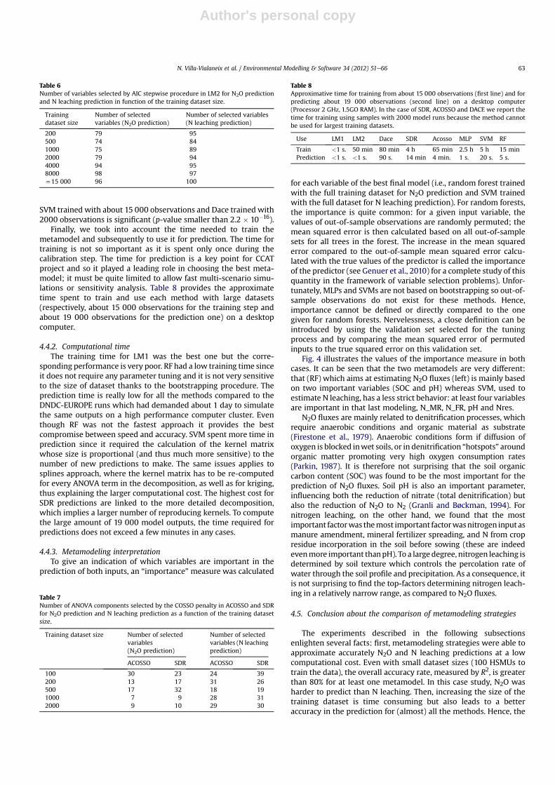
Finally, we took into account the time needed to train themetamodel and subsequently to use it for prediction. The time fortraining is not so important as it is spent only once during thecalibration step. The time for prediction is a key point for CCATproject and so it played a leading role in choosing the best meta-model; it must be quite limited to allow fast multi-scenario simu-lations or sensitivity analysis. Table 8 provides the approximatetime spent to train and use each method with large datasets(respectively, about 15 000 observations for the training step andabout 19 000 observations for the prediction one) on a desktopcomputer.

4.4.2. Computational timeThe training time for LM1 was the best one but the corre-

sponding performance is very poor. RF had a low training time sinceit does not require any parameter tuning and it is not very sensitiveto the size of dataset thanks to the bootstrapping procedure. Theprediction time is really low for all the methods compared to theDNDC-EUROPE runs which had demanded about 1 day to simulatethe same outputs on a high performance computer cluster. Eventhough RF was not the fastest approach it provides the bestcompromise between speed and accuracy. SVM spent more time inprediction since it required the calculation of the kernel matrixwhose size is proportional (and thus much more sensitive) to thenumber of new predictions to make. The same issues applies tosplines approach, where the kernel matrix has to be re-computedfor every ANOVA term in the decomposition, as well as for kriging,thus explaining the larger computational cost. The highest cost forSDR predictions are linked to the more detailed decomposition,which implies a larger number of reproducing kernels. To computethe large amount of 19 000 model outputs, the time required forpredictions does not exceed a few minutes in any cases.

4.4.3. Metamodeling interpretationTo give an indication of which variables are important in the

prediction of both inputs, an “importance” measure was calculated

for each variable of the best final model (i.e., random forest trainedwith the full training dataset for N2O prediction and SVM trainedwith the full dataset for N leaching prediction). For random forests,the importance is quite common: for a given input variable, thevalues of out-of-sample observations are randomly permuted; themean squared error is then calculated based on all out-of-samplesets for all trees in the forest. The increase in the mean squarederror compared to the out-of-sample mean squared error calcu-lated with the true values of the predictor is called the importanceof the predictor (see Genuer et al., 2010) for a complete study of thisquantity in the framework of variable selection problems). Unfor-tunately, MLPs and SVMs are not based on bootstrapping so out-of-sample observations do not exist for these methods. Hence,importance cannot be defined or directly compared to the onegiven for random forests. Nervelessness, a close definition can beintroduced by using the validation set selected for the tuningprocess and by comparing the mean squared error of permutedinputs to the true squared error on this validation set.

Fig. 4 illustrates the values of the importance measure in bothcases. It can be seen that the two metamodels are very different:that (RF) which aims at estimating N2O fluxes (left) is mainly basedon two important variables (SOC and pH) whereas SVM, used toestimate N leaching, has a less strict behavior: at least four variablesare important in that last modeling, N_MR, N_FR, pH and Nres.

N2O fluxes are mainly related to denitrification processes, whichrequire anaerobic conditions and organic material as substrate(Firestone et al., 1979). Anaerobic conditions form if diffusion ofoxygen is blocked inwet soils, or in denitrification “hotspots” aroundorganic matter promoting very high oxygen consumption rates(Parkin, 1987). It is therefore not surprising that the soil organiccarbon content (SOC) was found to be the most important for theprediction of N2O fluxes. Soil pH is also an important parameter,influencing both the reduction of nitrate (total denitrification) butalso the reduction of N2O to N2 (Granli and Bøckman, 1994). Fornitrogen leaching, on the other hand, we found that the mostimportant factorwas themost important factorwasnitrogen inputasmanure amendment, mineral fertilizer spreading, and N from cropresidue incorporation in the soil before sowing (these are indeedevenmore important thanpH). To a largedegree, nitrogen leaching isdetermined by soil texture which controls the percolation rate ofwater through the soil profile and precipitation. As a consequence, itis not surprising to find the top-factors determining nitrogen leach-ing in a relatively narrow range, as compared to N2O fluxes.

4.5. Conclusion about the comparison of metamodeling strategies

The experiments described in the following subsectionsenlighten several facts: first, metamodeling strategies were able toapproximate accurately N2O and N leaching predictions at a lowcomputational cost. Even with small dataset sizes (100 HSMUs totrain the data), the overall accuracy rate, measured by R2, is greaterthan 80% for at least one metamodel. In this case study, N2O washarder to predict than N leaching. Then, increasing the size of thetraining dataset is time consuming but also leads to a betteraccuracy in the prediction for (almost) all the methods. Hence, the

Table 6Number of variables selected by AIC stepwise procedure in LM2 for N2O predictionand N leaching prediction in function of the training dataset size.

Trainingdataset size

Number of selectedvariables (N2O prediction)

Number of selected variables(N leaching prediction)

200 79 95500 74 841000 75 892000 79 944000 94 958000 98 97x15 000 96 100

Table 7Number of ANOVA components selected by the COSSO penalty in ACOSSO and SDRfor N2O prediction and N leaching prediction as a function of the training datasetsize.

Training dataset size Number of selectedvariables(N2O prediction)

Number of selectedvariables (N leachingprediction)

ACOSSO SDR ACOSSO SDR

100 30 23 24 39200 13 17 31 26500 17 32 18 191000 7 9 28 312000 9 10 29 30

Table 8Approximative time for training from about 15 000 observations (first line) and forpredicting about 19 000 observations (second line) on a desktop computer(Processor 2 GHz, 1.5GO RAM). In the case of SDR, ACOSSO and DACE we report thetime for training using samples with 2000 model runs because the method cannotbe used for largest training datasets.

Use LM1 LM2 Dace SDR Acosso MLP SVM RF

Train <1 s. 50 min 80 min 4 h 65 min 2.5 h 5 h 15 minPrediction <1 s. <1 s. 90 s. 14 min 4 min. 1 s. 20 s. 5 s.



selection of a metamodeling approach has to be based on a carefulcompromise between computational costs and accuracy. Thischoice strictly depends on the size of available training data and onthe project’s target. We pointed out that splines and kriging basedmethods should be chosen when the number of training data issmaller than 2000 since they provided the most accurate solutionwith a reasonable running time. With large datasets, randomforests were able to handle the training step and to calculateaccurate predictions with low computational costs (more than15 000 observations were trained in about 15 min and only severalseconds were needed in predicting 19 000 new values).

Finally, we pointed out, in Section 4.4.3, that combining meta-modeling with an importance measure can also be used to providea simplified insight on the important processes and on the maininput variables involved in the prediction of N2O fluxes and Nleaching. This can help to find strategies to control nitrogen surplusor to perform a fast sensitivity analysis. This last issue is currentlyunder investigation.

5. Conclusion

This article provides a full comparison of several metamodelapproaches for the prediction of N2O fluxes and N leaching fromEuropean farmlands. The conclusions of the metamodel compar-ison are general enough to be extended to other similar casestudies. A more valuable and detailed impact assessment of CCstandards at European or country level is possible only by simu-lating all the 207 000 HSMUs that cover the EU27. This approachdemands the collection of enormous amounts of data and theirstorage into large datasets. From our work, random forest proved tobe a reliable and effective tool for elaborating large datasets withlow computational costs and an acceptable accuracy. For thesereasons it has been chosen to be integrated into the CCAT platformto estimate the N2O fluxes and N leaching from the EU27 farmlands.

References

Akaike, H., 1974. A new look at the statistical model identification. IEEE Transactionson Automatic Control 19, 716e723.

Alliance Environnement, 2007. Evaluation of the Application of Cross Compliance asForeseen under Regulation 1782/2003. Part I: Descriptive Report. TechnicalReport. D.G. Agriculture. Institute for European Environmental Policy (IEEP),London, UK and Orade-Brche Sarl, Auzeville, France.

Amit, Y., Geman, D., 1997. Shape quantization and recognition with random trees.Neural Computation 9, 1545e1588.

Anderson, M., Kustas, W., Norman, J., 2003. Upscaling and downscaling e a regionalview of the soil-plant-atmosphere continuum. Agronomy Journal 95,1408e1423.

Askegaard, M., Olesen, J., Kristensen, K., 2005. Nitrate leaching from organic arablecrop rotations: effects of location, manure and catch crop. Soil Use andManagement 21, 181e188.

Berlinet, A., Thomas-Agnan, C., 2004. Reproducing Kernel Hilbert Spaces in Prob-ability and Statistics. Kluwer Academic Publisher, Boston, Norwell, MA, USA/Dordrecht, The Netherlands.

Bishop, C., 1995. Neural Networks for Pattern Recognition. Oxford University Press,New York, USA.

Blanning, R., 1975. The construction and implementation of metamodels. Simula-tion 24, 177e184.

Boser, B., Guyon, I., Vapnik, V., 1992. A training algorithm for optimal marginclassifiers. In: Haussler, D. (Ed.), 5th Annual ACM Workshop on COLT. ACMPress, pp. 144e152.

Bouzaher, A., Lakshminarayan, P., Cabe, R., Carriquiry, A., Gassman, P., Shogren, J.,1993. Metamodels and nonpoint pollution policy in agriculture. WaterResources Research 29, 1579e1587.

Breiman, L., 2001. Random forests. Machine Learning 45, 5e32.Breiman, L., Friedman, J., Olsen, R., Stone, C., 1984. Classification and Regression

Trees. Chapman and Hall, New York, USA.Britz, W., 2008. Automated model linkages: the example of CAPRI. Agrarwitschaft

57, 363e367.Britz, W., Leip, A., 2009. Development of marginal emission factors for N losses from

agricultural soils with the DNDC-CAPRI metamodel. Agriculture, Ecosystemsand Environment 133, 267e279.

Britz, W., Witzke, P., 2008. CAPRI Model Documentation 2008. Online at:. CAPRIProject, Institute for Food and Resource Economics, Bonn, Germany http://www.capri-model.org/.

Chadwick, D., 2005. Emissions of ammonia, nitrous oxide and methane from cattlemanure heaps: effect of compaction and covering. Atmospheric Environment39, 787e799.

Chang, C., Lin, C., 2001. LIBSVM: A Library for Support Vector Machines. Softwareavailable at. http://www.csie.ntu.edu.tw/cjlin/libsvm.

Christmann, A., Steinwart, I., 2007. Consistency and robustness of kernel-basedregression in convex risk minimization. Bernouilli 13, 799e819.

Cressie, N., 1990. The origins of kriging. Mathematical Geology 22, 239e352.De Vries, W., Kros, H., Velthof, G., Oudendag, D., Leip, A., van der Velde, M., Kempen,

M., 2008. Development and application methodology of environmental impacttool to evaluate cross compliance measures. Technical Report Deliverable 4.2.1of EU STREP 44423 (CCAT Project).

Del Grosso, S., Parton, W., Mosier, A., Walsh, M., Ojima, D.S., Thornton, P., 2006.DAYCENT national-scale simulation of nitrous oxide emissions from croppedsoils in the United States. Journal of Environment Quality 35, 1451e1460.

Dimopoulus, D., Fermantziz, I., Vlahos, G., 2007. The Responsiveness of CrossCompliance Standards to Environmental Pressure. Agricultural University ofAthens, Athens, Greece. Technical Report Deliverable 12 of the CC NetworkProject, SSPE-CT-2005-022727.

Elbersen, B., Jongeneel, R., Kempen, M., Klein-Lankhorst, R., De Vries, W., Lesschen,J., Onate, J., Alonso, M., Kasperczyk, N., Schramek, J., Mik, M., Peepson, A.,Bouma, F., Staritsky, I., Kros, H., 2010. Final Report of CCAT Project Results.Technical Report Deliverable 2.8 of EU STREP 44423-CCAT (CCAT project).

European Council, 1991. Nitrate Directive 91/676/EEC. Technical Report. EuropeanUnion, Brussels, Belgium.

European Council, 2000. Water Framework Directive 2000/60/EC. Technical Report.European Union, Brussels, Belgium.

European Council, 2003. Council Regulation (EC). Technical Report 1782/2003.European Union, Brussels, Belgium.

European Council, 2009. Council Regulation (EC) No 73/2009. Technical Report.European Council, Brussels, Belgium.

European Commission, 2002. Implementation of Council Directive 91/676/EECConcerning the Protection of Waters against Pollution Caused by Nitrates from

Fig. 4. Importance measure for each variable in the case of (left) N2O prediction with the full training dataset and random forest and of (right) N leaching prediction with the fulltraining dataset and SVM (for the meaning of the acronyms, please refer to Section 4.2).



Agricultural Sources. European Commission, Luxembourg. Technical Report.D.G. Environment.

European Environment Agency, 1995. Europe’s Environment, the Dobriss Assess-ment. European Environment Agency. Technical Report.

European Environment Agency, 2010. Annual European Community GreenhouseInventory 1980-2008 and Inventory Report 2010. Submission to the UNFCCC Secre-tariat. Technical Report. European Environment Agency, Copenhagen, Denmark.

European Union Commission, 2004. Commission Regulation No 796/2004. Euro-pean Commission, Brussels, Belgium. Technical Report.

European Union Commission, 2009. Commission Regulation No 1122/2009. Euro-pean Commission, Brussels, Belgium. Technical Report.

European Union Commission, 2010. Agriculture in the EU e Statistical andEconomic Information e Report 2009. European Commission, Brussels,Belgium. Technical Report.

FAO, 2005. Key to Drought-resistant Soil and Sustained Food Production. TheImportance of Soil Organic Matter. Food Agricultural Organization, Rome, Italy.Technical Report Soils bulletin 80.

FAO, 2007. Payer les agriculteurs pour les services environnmentaux. La situationmondiale de l’alimentation et de l’agriculture. Food Agricultural Organization,Rome, Italy. Technical Report.

Firestone, M., Smith, M., Firestone, R., Tiedje, J., 1979. The influence of nitrate,nitrite, and oxygen on the composition of the gaseous products of dentrificationin soil. Soil Science Society of America Journal 43, 1140e1144.

Follador, M., Leip, A., 2009. Derivation of DNDC Meta-models to Evaluate the Impactof Cross Compliance Measures on Nitrogen N Surplus, N Leaching, N2O Emis-sions at European Scale. European Commission, D.G Joint Research Centre,Institute for Environment and Sustainability, Climate Change Unit, Ispra, Italy.Technical Report Deliverable 4.2.3 of EU STREP 44423-CCA.

Follador, M., Leip, A., Orlandini, L. Assessing the impact of cross compliancemeasures on nitrogen fluxes from European farmlands with DNDC-EUROPE.Environmental Pollution, in press, doi:10.1016/j.envpol.2011.01.025.

Forrester, A., Keane, A., 2009. Recent advances in surrogate-based optimization.Progress in Aerospace Sciences 45, 50e79.

Friedman, J.,1991.Multivariate adaptive regression splines. Annals of Statistics 19,1e67.Genuer, R., Poggi, J., Tuleau-Malot, C., 2010. Variable selection using random forests.

Pattern Recognition Letters 31, 2225e2236.Granli, T., Bøckman, O., 1994. Nitrous Oxide from Agriculture. In: Norwegian Journal

of Agricultural Sciences Supplement No. 12. Norsk Hydro Research Centre,Porsgrunn, Norway.

Gu, C., 2002. Smoothing Spline ANOVA Models. Springer-Verlag, New York, USA.Haberlandt, U., Krysanova, V., Bardossy, A., 2002. Assessment of nitrogen leaching

from arable land in large river basins. Part II: regionalisation using fuzzy rulebased modelling. Ecological Modelling 150, 277e294.

Ho, T., 1998. The random subspace method for constructing decision forests. IEEETransactions on Pattern Analysis and Machine Intelligence 20, 832e844.

Hornik, K., 1991. Approximation capabilities of multilayer feedfoward networks.Neural Networks 4, 251e257.

Intergovernmental Panel on Climate Change, 2007. Fourth Assessment Report of theIntergovernmental Panel on Climate Change. Working Group I e The PhysicalScience Basis. Cambridge University Press, Cambridge, United Kingdom/NewYork, NY, USA.

Jongeneel, R., Elbersen, B., de Vries, V., Klein-lankhorst, J., Schramek, J., Rudloff, B.,Heckelei, T., Kempen, M., Annen, D., van der Velde, M., Leip, A., Redman, M.,Mikk, M., Onate, J., Slangen, L., 2007. General Approach to the Assessment of theImpacts of CC in the EU and List of Indicators Technical Report Deliverables 2.1and 2.2 of EU STREP 44423. CCAT Project.

Jongeneel, R., Elbersen, B., Klein-Lankhorst, R., De Vries, W., Kros, H., Velthof, G.,Kempen, M., Annen, D., Onate, J., van der Velde, M., Leip, A., 2008. ReportDescribing the Operationalisation of the First Selection of Indicators intoImpacts of Cross Compliance for the Implementation in the First Prototype ofthe Analytical Tool Technical Report Deliverable 2.3 of EU STREP 44423-CCAT.

Kalman, R., 1960. A new approach to linear filtering and prediction problems.Transactions of the ASME, Journal of Basic Engineering 82D, 35e45.

Keerthi, S., Shevade, S., Bhattacharyya, C., Murty, K., 2001. Improvements to platt’sSMO algorithm for SVM classifier design. Neural Computation 13, 637e649.

Kennedy, M., O’Hagan, A., 2001. Bayesian calibration of computer models (withdiscussion). Journal of the Royal Statistical Society, Series B 63, 425e464.

Kirchmann, H., Esala, M., Morken, J., Ferm, M., Bussink, W., Gustavsson, J.,Jakobsson, C., 1998. Ammonia emissions from agriculture. Nutrient Cycling inAgroecosystems 51, 1e3.

Kleijnen, J., 1975. A comment on Blanning’s “Metamodel for sensitivity analysis: theregression metamodel in simulation”. Interfaces 5, 21e23.

Kleijnen, J., 2009. Kriging metamodelin in simulation: a review. European Journal ofOperational Research 1992, 707e716.

Kleijnen, J., Sargent, R., 2000. A methodology for fitting and validating metamodelsin simulation. European Journal of Operational Research 120, 14e29.

Krogh, A., Hertz, J., 1992. A simple weight decay can improve generalization. In:Kaufmann, M. (Ed.), Advances in Neural Information Processing Systems, pp.950e957.

Krysanova, V., Haberlandt, U., 2002. Assessment of nitrogen leaching from arableland in large river basins. Part I: simulation experiments using a process-basedmodel. Ecological Modelling 150, 255e275.

Leip, A., Dämmgen, U., Kuikman, P., van Amstel, A., 2005. The quality of European(EU-15) greenhouse gas inventories from agriculture. Environmental Sciences 2,177e192.

Leip, A., Marchi, G., Koeble, R., Kempen, M., Britz, W., Li, C., 2008. Linking aneconomic model for european agriculture with a mechanistic model to estimatenitrogen and carbon losses from arable soils in europe. Biogeosciences 5,73e94.

Leip, A., Achermann, B., Billen, G., Bleeker, A., Bouwman, L., de Vries, W.,Dragosits, U., Döring, U., Fernall, D., Geupel, M., Johnes, P., Le Gall, A.C., Monni, S.,Neve�ce�ral, R., Orlandini, L., Prud’homme, M., Reuter, H., Simpson, D., Seufert, G.,Spranger, T., Sutton, M., van Aardenne, J., Voss, M., Winiwarter, W., 2011. Inte-grating nitrogen fluxes at the European scale. In: Sutton, M., Howard, C.,Erisman, J., Billen, G., Bleeker, A., van Grinsven, H., Grennfelt, P., Grizzetti, B.(Eds.), European Nitrogen Assessment. Cambridge University Press, New York,USA, pp. 345e376. chapter 16.

Leip, A., Britz, W., De Vries, W., Weiss, F. Farm, land, and soil nitrogen budgets foragriculture in Europe. Environmental Pollution, in press a, doi:10.1016/j.envpol.2011.01.040.

Leip, A., Busto, M., Winiwarter, W. Developing stratified N2O emission factors forEurope. Environmental Pollution, in press b, doi:10.1016/j.envpol.2010.11.024.

Li, C., 2000. Modeling trace gas emissions from agricultural ecosystems. NutrientCycling in Agroecosystems 58, 259e273.

Li, C., Frolking, S., Frolking, T., 1992. Model of nitrous oxide evolution from soildriven by rainfall events: 1, model structure and sensitivity. Journal ofGeophysical Research 97, 9759e9776.

Lin, Y., Zhang, H., 2006. Component selection and smoothing in smoothing splineanalysis of variance models. Annals of Statistics 34, 2272e2297.

Lophaven, S., Nielsen, H., Sondergaard, J., 2002. DACE e A Matlab KrigingToolbox, Version 2.0. Technical Report IMM-TR-2002-12. Informatics andMathematical Modelling, Technical University of Denmark, DK-2800 Kgs.Lyngby, Denmark.

Matson, P., Parton, W., Power, A., Swift, M., 1997. Agricultural intensification andecosystem properties. Science 277, 504e509.

Mattera, D., Haykin, S., 1998. Support vector machines for dynamic reconstructionof a chaotic system. In: Schölkopf, B., Burges, C., Smola, A. (Eds.), Advances inKernel Methods: Support Vector Learning. MIT Press, Cambridge, MA, USA, pp.209e241.

Meckesheimer, M., Booker, A., Barton, R., Simpson, T., 2002. Computationallyinexpensive metamodel assessment strategies. AIAA Journal 40, 2053e2060.

Montès, P., 1994. Smoothing noisy data by kriging with nugget effects. In:Laurent, P., Le Méhauté, A., Shumaker, L., Peters, A. (Eds.), Wavelets, Images andSurface Fitting. AK Peters, Wellesley, MA, USA, pp. 371e378.

Ng, C., Young, P., 1990. Recursive estimation and forecasting of non-stationary timeseries. Journal of Forecasting 9, 173e204.

Oenema, O., Oudendag, D., Velthof, G., 2007. Nutrient losses from manuremanagement in the European Union. Livestock Science 112, 261e272.

Oenema, O., Witzke, H., Klimont, Z., Lesschen, J., Velthof, G., 2009. Integratedassessment of promising measures to decrease nitrogen losses from agriculturein EU-27. Agriculture, Ecosystems and Environment 133, 280e288.

Parkin, T., 1987. Soil microsites as a source of denitrification variability. Soil ScienceSociety of America Journal 51, 1194e1199.

Pineros Garcet, J., Ordonez, A., Roosen, J., Vanclooster, M., 2006. Metamodeling:theory, concepts and application to nitrate leaching modelling. EcologicalModelling 193, 629e644.

Power, A., 2010. Ecosystem services and agriculture: tradeoffs and synergies. Phil-osofical Transactions of the Royal Society B 365, 2959e2971.

Ratto, M., Pagano, A., 2010. Recursive algorithms for efficient identification ofsmoothing spline anova models. Advances in Statistical Analysis 94, 367e388.

Ratto, M., Pagano, A., Young, P.C., 2007. State dependent parameter meta-modellingand sensitivity analysis. Computer Physics Communications 177, 863e876.

Ripley, B., 1994. Neural networks and related methods for classification. Journal ofthe Royal Statistical Society, Series B 56, 409e456.

Sacks, J., Welch, W., Mitchell, T., Wynn, H., 1989. Design and analysis of computerexperiments. Statistical Science 4, 409e435.

Santner, T., Williams, B., Notz, W., 2003. The Design and Analysis of ComputerExperiments. Springer, New York, NY, USA.

Scherr, S., Sthapit, S., 2009. Farming and land use to cool the planet. In:Institute, T.W. (Ed.), State of World 2009. W.W. Norton & Co., Washington DC,USA, pp. 30e49. chapter 3.

Schwarz, G., 1978. Estimating the dimension of a model. Annals of Statistics 6,461e464.

Schweppe, F., 1965. Evaluation of likelihood functions for Gaussian signals. IEEETransactions on Information Theory 11, 61e70.

Shaffer,M.,Ma, L., 2001. Carbon andnitrogen dynamics in upland soils. In: Shaffer,M.,Ma, L., Hansen, S. (Eds.), Modeling Carbon and Nitrogen Dynamics for SoilManagement. CRC Press, LLC, Bacon Raton, Florida, USA, pp. 11e27. chapter 2.

Simpson, T., Peplinski, J., Koch, P., Allen, J., 2001. Metamodels for computer-basedengineering design: survey and recommendations. Engineering withComputers 17, 129e150.

Singh, R., 2000. Environmental consequences of agricultural development: a casestudy from the green revolution state of Haryana, India. Agriculture, Ecosystemsand Environment 82, 97e103.

Steinwart, I., Christman, A., 2008. Support Vector Machines. Information Scienceand Statistics.

Steinwart, I., Christmann, A., 2008. Support Vector Machines. Information Scienceand Statistics. Springer.

Storlie, C., Bondell, H., Reich, B., Zhang, H., 2011. Surface estimation, variableselection, and the nonparametric oracle property. Statistica Sinica 21, 679e705.



Tibshirani, R., 1996. Regression shrinkage and selection via the lasso. Journal of theRoyal Statistical Society, Series B 58, 267e288.

Tilman, D., Cassman, K., Matson, P., Naylor, R., Polasky, S., 2002. Agriculturalsustainability and intensive production practices. Nature 418, 671e677.

van Gighc, J., 1991. System Design Modeling and Metamodeling. Springer, New York,USA.

van Grinsven, H., Ward, M., Benjamin, N., De Kok, T., 2006. Does the Evidence aboutHealth Risks Associated with Nitrate Ingestion Warrant an Increase of theNitrate Standard for Drinking Water? Environmental Health: a Global AccessScience Source 5.

van der Velde, M., Bouraoui, F., de Vries, W., 2009. Derivation of EPIC Meta-modelsto Evaluate the Impact of Cross Compliance Measures on Leaching and Runoff ofNitrogen and Soil Erosion at European Scale CCAT Deliverable (report) 4.2.3.2.CCAT project.

Vanclooster, M., Viaene, P., Christiaens, K., Ducheyne, S., 1996.Wave: AMathematicalModel for Simulating Water and Agrochemicals in the Soil and Vadose Environ-ment, Reference and User’s Manual (Release 2.1). Institute for Land and WaterManagement, KatholiekeUniversiteit Leuven, Leuven, Belgium. Technical Report.

Vapnik, V., 1995. The Nature of Statistical Learning Theory. Springer Verlag,New York, USA.

Vapnik, V., 1998. Statistical Learning Theory. Wiley, New York, USA.Velthof, G., Oudendag, D., Witzke, H., Asman, W., Klimont, Z., Oenema, O., 2009.

Integrated assessment of nitrogen emissions from agriculture in EU-27 usingMITERRA-EUROPE. Journal of Environmental Quality 38, 1e16.

Venables, W., Ripley, B., 2002. Modern Applied Statistics with S-PLUS. Springer,New York, USA.

Wahba, G., 1990. Spline Models for Observational Data. Society for Industrial andApplied Mathematics, Philadelphia, Pennsylvania, USA.

Wang, G., Shan, S., 2007. Review of metamodeling techniques in support of engi-neering design optimization. Journal of Mechanical Design 129, 370e380.

Webb, J., Menzi, H., Pain, B., Misselbrook, T., Dämmgen, U., Hendriks, H., Döhler, H.,2005. Managing ammonia emissions from livestock production in Europe.Environmental Pollution 135, 399e406.

Werbos, P., 1974. Beyond Regression: New Tools for Prediction and Analysis inBehavior Sciences. Ph.D. thesis. Commitee on Applied Mathematics, HarvardUniversity. Cambridge, MA, USA.

Young, P., 1999. Nonstationary time series analysis and forecasting. Progress inEnvironmental Science 1, 3e48.

Young, P., 2000. Stochastic, dynamic modelling and signal processing: time variableand state dependent parameter estimation. In: Fitzgerald, W., Walden, A.,Smith, R., Young, P. (Eds.), Nonlinear and Nonstationary Signal Processing.Cambridge University Press, Cambridge, USA, pp. 74e114.

Young, P., 2001. The identification and estimation of nonlinear stochastic systems.In: Mees, A. (Ed.), Nonlinear Dynamics and Statistics. Birkhauser, Boston, USA,pp. 127e166.

Young, P., Ng, C., 1989. Variance intervention. Journal of Forecasting 8, 399e416.Zhang, Y., Li, C., Zhou, X., Moore, B., 2002. A simulation model linking crop growth and

soil biogeochemistry for sustainable agriculture. EcologicalModelling 151, 75e108.


A comparison of eight metamodeling techniques for the simulation of N 2 O fluxes and N leaching from...

Documents

Transcript of A comparison of eight metamodeling techniques for the simulation of N 2 O fluxes and N leaching from...