a comparison between stock assessment - RUA

EDUARDO SÁNCHEZ LLAMASSeptiembre 2017

A comparison between stock assessment methods and assessment of management scenarios: a practical study case for European hake in GSA’s 12 – 16.

Calculation of reference points in decreasing trend populations

TESISpresentada y públicamente defendidapara la obtención del título de

MASTER OF SCIENCE

Máster Internacional enGESTIÓN PESQUERA SOSTENIBLE

(6ª edición: 2015-2017)

A COMPARISON BETWEEN STOCK ASSESSMENT

METHODS AND ASSESSMENT OF MANAGEMENT

SCENARIOS: A PRACTICAL STUDY CASE FOR

EUROPEAN HAKE IN GSA’s 12 – 16

CALCULATION OF REFERENCE POINTS IN DECREASING

TREND POPULATIONS

EDUARDO SÁNCHEZ LLAMAS

TESIS PRESENTADA Y PUBLICAMENTE DEFENDIDA PARA LA OBTENCIÓN

DEL TITULO DE MASTER OF SCIENCE EN

GESTIÓN PESQUERA SOSTENIBLE

Alicante a 01 de Septiembre de 2017

MASTER EN GESTIÓN PESQUERA SOSTENIBLE

(6ª edición: 2015-2017)

A COMPARISON BETWEEN STOCK ASSESMENT





TREND POPULATIONS

EDUARDO, SÁNCHEZ LLAMAS

Trabajo realizado en General Fisheries Commission for the Mediterranean (GFCM), bajo la dirección de Miguel Bernal y junto con la Universidad de Vigo bajo la dirección de José María da Rocha.

Y presentado como requisito parcial para la obtención del Diploma Master of Science en Gestión Pesquera Sostenible otorgado por la Universidad de Alicante a través de Facultad de Ciencias y el Centro Internacional de Altos Estudios Agronómicos Mediterráneos (CIHEAM) a través del Instituto Agronómico Mediterráneo de Zaragoza (IAMZ).

Vº Bº Director Vº Bº Director Autor

Fdo: D. José María da Rocha . Fdo: D. Miguel Bernal Fdo: D. Eduardo Sánchez Llamas

a 01 de Septiembre de 2017

A COMPARISON BETWEEN STOCK ASSESMENT





TREND POPULATIONS

EDUARDO, SÁNCHEZ LLAMAS

Trabajo realizado en General Fisheries Commission for the Mediterranean (GFCM), bajo la dirección de Miguel Bernal y junto con la Universidad de Vigo bajo la dirección de José María Da Rocha.

Presentado como requisito parcial para la obtención del Diploma Master of Science en Gestión Pesquera sostenible otorgado por la Universidad de Alicante a través de Facultad de Ciencias y el Centro Internacional de Altos Estudios Agronómicos Mediterráneos (CIHEAM) a través del Instituto Agronómico Mediterráneo de Zaragoza (IAMZ). Esta Tesis fue defendida el día 27 de septiembre de 2017 ante un Tribunal Formado por - José Luis Sánchez Lizaso - Maria Grazia Pennino - José Jacobo Zubcoff - Bernardo Basurco

Agradecimientos

En primer lugar, me gustaría agradecer al Dr. José Luís Sánchez Lizaso todo su esfuerzo

y dedicación a la hora de mantener y organizar el máster. Intentando en todo momento buscar

lo mejor para sus alumnos. Sin su ayuda, confianza y transmisión de conocimientos este trabajo

no habría sido posible.

En segundo lugar, al Dr. Miguel Bernal por ser un ejemplo de trabajo y profesionalidad

a lo largo del pasado año. Transmitiéndome sus conocimientos y permitiendo mi aprendizaje

durante las numerosas actividades en las que me ha hecho partícipe en las oficinas de

FAO/GFCM y en las numerosas reuniones en las que hemos estado infinitas horas. Él, junto

con todo el equipo de la GFCM me han hecho sentir uno más del grupo a lo largo del desarrollo

del trabajo permitiéndome evolucionar tanto en el terreno personal cómo en el profesional.

También me gustaría agradecer al Dr. José María Da Rocha la continua disposición a lo

largo del desarrollo del proyecto. Pese a las dificultades iniciales siempre ha estado ahí

ayudándome con el proyecto y consiguiendo, estando cada uno en una parte del mundo, que la

calidad del trabajo no se viese alterada.

Tampoco hay que olvidar todos los expertos que me han ayudado a lo largo de este

trabajo. Vita Gancitano proporcionándome los datos ha sido fundamental, así como todos los

expertos del WGSAD que me han aportado cada uno su granito de arena a lo largo del desarrollo

del proyecto y me han proporcionado ideas para una continua mejora. En especial (aunque

también incluida en el personal de la GFCM) a Betulla Morello por animarme y ayudarme en

los momentos en los que quería lanzar el ordenador por la ventana. Muchas gracias.

Por último y tal vez más importante, a mi familia por darlo todo durante el pasado año

y ayudarme a lo largo de todo mi proceso de formación sacando recursos de dónde no los había.

Sin ellos, nada de este trabajo habría sido posible. Han sido parte fundamental de este trabajo y

de todos los éxitos futuros.

Muchas gracias a todos.

Content

Content ...............................................................................................................................................9

Figures Index .................................................................................................................................... 13

Tables Index ..................................................................................................................................... 17

Acronyms Table ............................................................................................................................... 19

Abstract ............................................................................................................................................ 21

Resumen ........................................................................................................................................... 23

Chapter 1: A Comparison Between Stock Assessment Methods and Assessment of Management

Scenarios: A Practical Study Case for European Hake in GSA’s 12 – 16 ..................................... 25

1.- Introduction ..............................................................................................................................1

1.1.- State and management of Mediterranean fisheries resources ..............................................4

1.2.- The role of the General Fisheries Commission for the Mediterranean (GFCM) ..................5

1.2.1.- Working group on demersal species (WGSAD) .........................................................8

1.2.2.- Working group on management strategy evaluation (WKMSE)..................................8

1.2.3.- Subregional committee central Mediterranean (SRC-CM) ..........................................8

1.3.- Structure and objectives of this thesis ................................................................................8

2.- Methods .................................................................................................................................. 11

2.1.- Target Stocks and Study area ........................................................................................... 11

2.2.- Input Data ....................................................................................................................... 13

2.3.- Stock assessment methods ............................................................................................... 14

2.3.1.- Extended Survival Analysis (XSA) .......................................................................... 15

2.3.2.- Assessment for all (a4a) ........................................................................................... 16

2.4.- Reference Points ............................................................................................................. 20

2.4.1.- Short-Term Forecasts ............................................................................................... 21

2.5.- MSE ................................................................................................................................ 22

3.- Results .................................................................................................................................... 25

3.1.- Stock Assessment ............................................................................................................ 25

3.1.1.- XSA Results ............................................................................................................ 25

3.1.2.- Deterministic Assessment for All (a4a) .................................................................... 27

3.1.3.- Comparison a4a vs XSA .......................................................................................... 31

3.1.4.- Stochastic Assessment for All (a4a) ......................................................................... 32

3.2.- Short term forecast .......................................................................................................... 34

3.2.1.- XSA ........................................................................................................................ 34

3.2.2.- Deterministic a4a ..................................................................................................... 36

3.3.- Medium-Long term forecast and assessment of management scenarios ............................ 38

3.3.1.- XSA ........................................................................................................................ 38

3.3.2.- Deterministic a4a ..................................................................................................... 38

3.3.3.- Stochastic a4a .......................................................................................................... 39

4.- Discussion .............................................................................................................................. 43

4.1.- Stock assessment results and advice................................................................................. 43

4.2.- Uncertainty in Stock Assessment: Stochastic a4a ............................................................. 44

4.3.- Assessment of Management Scenarios ............................................................................. 45

4.4.- Mediterranean Sea: Status and future ............................................................................... 46

5.- Conclusion .............................................................................................................................. 49

6.- Future steps............................................................................................................................. 51

Chapter 2: Calculation of Reference Points in Decreasing Trend Populations ............................ 55

1.- Introduction ............................................................................................................................ 57

2.- Methods .................................................................................................................................. 59

2.1.- Data Acquisition and Study area ...................................................................................... 59

2.2.- Stock Dynamics .............................................................................................................. 60

2.3.- Recruitment Analysis ...................................................................................................... 61

2.4.- Fishery management: The role of λ parameter and effects of different 𝛽 over the regulator

......................................................................................................................................................... 62

2.5.- Yield ............................................................................................................................... 65

2.6.- Harvest control rules and risk .......................................................................................... 65

2.7.- Trend effects over reference points .................................................................................. 67

3.- Results ......................................................................................................................................... 69

3.1.- Recruitment analysis ....................................................................................................... 69

3.2.- Fmax and yield .................................................................................................................. 70

3.3.- Comparison of Harvest Control Rules: Constant effort versus Biological based catch. ..... 71

4.- Discussion ................................................................................................................................... 73

5.- Conclusions ................................................................................................................................. 75

References ........................................................................................................................................ 77

Annex – Codes Chapter 1.................................................................................................................. 85

1.- Extended Survivor Analysis .................................................................................................... 85

2.- Deterministic a4a .................................................................................................................... 91

3.- Stochastic a4a Analysis ........................................................................................................... 97

4.- Short Term Forecasting ......................................................................................................... 110

5.- Long/Medium Term Forecasting ........................................................................................... 120

Annex – Codes Chapter 2................................................................................................................ 174

Figures Index

Chapter 1: A Comparison Between Stock Assessment Methods and Assessment of Management

Scenarios: A Practical Study Case for European Hake in GSA’s 12 – 16.

Figure 1 - Landings % in the Mediterranean and Black Sea (Last 10 years), (GFCM, 2016). ..........1

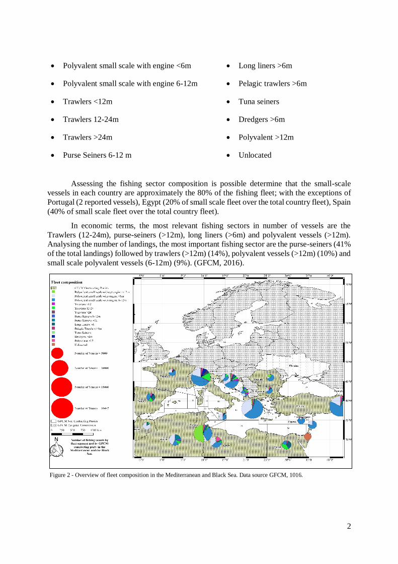
Figure 2 - Overview of fleet composition in the Mediterranean and Black Sea. Data source GFCM,

1016. ..................................................................................................................................................2

Figure 3 - Mediterranean fleet composition. Data source GFCM 2016. ...........................................3

Figure 4 - Average overexploitation index (Fcurr/Ftarget) for the main commercial species in the

Mediterranean and Black Sea. .............................................................................................................4

Figure 5 - General Fisheries Commission for the Mediterranean members. .....................................5

Figure 6 . GFCM provision of advice and decision-making process. ...............................................6

Figure 7 - GFCM Mid-Term Strategy. (GFCM 2016) .....................................................................8

Figure 8 - Study area: GFCM GSA's 12, 13, 14, 15, 16................................................................. 12

Figure 9 - Catch trends during the timeseries in GSA 12 -16......................................................... 13

Figure 10 - Length frequency distribution for MEDITS trawl survey 2007-2015 in percentage for

GSA 15 (left handed side) and GSA 16 (Right handed side) in number of individuals. ...................... 14

Figure 11 - Process of a4a approach. (Jardim et al., 2017). ........................................................... 17

Figure 12 - Marginal distributions of each growth parameter using multivariate normal distribution.

......................................................................................................................................................... 18

Figure 13 - Growth Curve with a multivariate normal distribution ................................................ 18

Figure 14 - Natural mortality by age and year ............................................................................... 19

Figure 15 - Sustainability from an advisory point of view. ............................................................ 21

Figure 16 - Conceptual overview of the management strategy evaluation modelling process.

Modified from Betulla Morello WKMSE. ......................................................................................... 22

Figure 17 - European hake XSA control objects (Left-handed side) and XSA shrinkages (Right-

handed side). ..................................................................................................................................... 25

Figure 18 - European hake in GSA 12-16. Estimates of recruitment, SSB, Catch and F for the final

run .................................................................................................................................................... 26

Figure 19 - European hake in GSA 12 -16. XSA. Diagnostics for the best run for shrk.age=1. Log

Residuals of the best XSA configuration analysis (left), retrospective analysis (right). ....................... 26

Figure 20 - European Hake GSA 12-16 Summary of the yield per recruit analysis (Y/R) results. .. 27

Figure 21 - European hake in GSA 12-16. Estimates of recruitment, SSB, Catch and F for

deterministic a4a final run. ................................................................................................................ 28

Figure 22 - European Hake GSA 12-16. Coefficient of determination diagnostics shows a problem

in index related data values. Ages 0 and 1 presented problems in fitting. ........................................... 29

Figure 23 - European hake, GSA 12-16. Deterministic a4a diagnostics results. ............................. 29

Figure 24 - European hake in GSA 12 -16. Bubble plot, Deterministic a4a assessment residuals. .. 30

Figure 25 - Quantile plot of log residuals diagnostics shows a good fitting level in the stock

assessment diagnostics. ..................................................................................................................... 30

Figure 26 - European Hake GSA 12-16 Summary of the yield per recruit analysis (Y/R) results. .. 31

Figure 27 - European hake GSA 12 - 16. XSA and a4a results comparison. .................................. 31

Figure 28 - European hake GSA 12-16. Stochastic a4a results. ..................................................... 32

Figure 29 - European hake GSA 12-16. Stochastic a4a results. ..................................................... 32

Figure 30 - XSA short term forecast. ............................................................................................ 35

Figure 31 - Deterministic a4a short term forecast ......................................................................... 37

Figure 32 - XSA Forecasting and assessment of management scenarios. ....................................... 40

Figure 33 - Deterministic a4a forecasting and assessment of management scenarios. .................... 41

Figure 34 - Stochastic a4a forecasting and assessment of management scenarios. ......................... 42

Chapter 2: Calculation of Reference Points in Decreasing Trend Populations

Figure 35 - Study area ICES VIIIc and IXa areas.......................................................................... 59

Figure 36 - System dynamics ....................................................................................................... 60

Figure 37 - Hodrick and Prescott filter residuals. .......................................................................... 62

Figure 38 - Different kinds of decision rules as a function of the weight parameter λ in the managers

objective function. ............................................................................................................................ 62

Figure 39 - Different strategies to achieve the target comparison. ................................................. 63

Figure 40 - Standard error comparison. Constant F Vs Lambda > 0 .............................................. 67

Figure 41 - Different sustainable management areas between both strategies. ............................... 67

Figure 42 - Recruitment trend ...................................................................................................... 69

Figure 43 - Isolated recuitment trend ............................................................................................ 69

Figure 44 - Top left panel shows differences between recruitment and trend. Bottom left shows

cyclical component of the recruitment series. Top right shows the soft recruitment series removing the

trend from the series.......................................................................................................................... 70

Figure 45 - Fmax reference point ................................................................................................. 70

Figure 46 - Different Safe fishing areas for both HCR strategies. In lambda > 0 we could see that the

safe fishing area is bigger than in Constant F strategy. ....................................................................... 72

Figure 47 - Results of the 1000 HCR simulations. Top graph represents the possible fishing mortality

fluctuations under a biomass based harvest control rule during 25 simulated years. Bottom graph

represents the fluctuations in target spawning stock biomass / cur ..................................................... 72

Tables Index

Chapter 1: A Comparison Between Stock Assessment Methods and Assessment of

Management Scenarios: A Practical Study Case for European Hake in GSA’s 12 – 16.

Table 1 - GFCM list of priority species ..........................................................................................7

Table 2 - Stock unit and main information .................................................................................... 12

Table 3 - Trawl survey sampling area and number of hauls (GSA 16 in 2014) .............................. 14

Table 4 - XSA algorithm (Shepherd, 1992) .................................................................................. 15

Table 5 - XSA configuration ........................................................................................................ 16

Table 6 - Summary of data sources by model ............................................................................... 20

Table 7 - Management strategy evaluation process ....................................................................... 22

Table 8 - European hake GSA 12-16 XSA reference points .......................................................... 27

Table 9 - European hake GSA 12-16 Deterministic a4a reference points ...................................... 31

Table 10 - European hake GSA 12-16 Stochastic a4a reference points ......................................... 33

Table 11 - European Hake in GSA 12-16. XSA. Short term forecast under different F scenarios (3-

year average, 2013-2015) weight at age, maturity at age and F at age. Recruitment (age 0) geomean

2013-2015. ....................................................................................................................................... 34

Table 12 - European Hake in GSA 12-16. Deterministic a4a short term forecast under different F

scenarios (3-year average, 2013-2015) weight at age, maturity at age and F at age. Recruitment (age 0)

geomean 2013-2015 .......................................................................................................................... 36

Chapter 2: Calculation of Reference Points in Decreasing Trend Populations

Table 13 - Age structured model (ICES WGHANSA report 2015. Pag. 222) ................................ 59

Table 14 - Numerical experiment to evaluate the implications between HCR, reference points and

risk. .................................................................................................................................................. 71

Acronyms Table

A4a: Assessment for All

DCRF: Data Collection Reference Framework

F: Fishing Mortality

FAO: Food and Agriculture Organization

Flim: Fishing Mortality Limit

Fmax: Maximum Fishing Mortality

FMSY: Fishing Mortality at Maximum Sustainable Yield

FPR: Precautionary Fishing Mortality

GFCM: General Fisheries Commission for the Mediterranean

GSA: Geographical Subareas

HCR: Harvest Control Rule

H-P: Hodrick and Prescott

ICCAT: International Commission for the Conservation of Atlantic Tunas

ICES: International Council for the Exploration of the Sea

IPCC: Intergovernmental Panel on Climate Change

JRC: Joint Research Center

K: Fish Growth Parameter

L: Length

Linf: Length at Infinite

M: Natural Mortality

MSC: Marine Stewardship Council

MSE: Management Strategy Evaluation

N: Number of Individuals

SAC: Scientific Advisory Committee

SOP: Sum of Squares

SRC-CM: Subregional Committee Central Mediterranean

SSB: Spawning Stock Biomass

STECF: Scientific, Technical and Economic Committee for Fisheries

TSB: Total Spawning Biomass

UNEP/MAP: United Nations Environment Programme

VPA: Virtual Population Analysis

WGHANSA: Working Group on Southern Horse Mackerel, Anchovy and Sardine

WGSA’s: Working Group on Stock Assessment

WGSAD: Working Group on Demersal Species

WKMSE: Working Group on Management Strategy Evaluation

XSA: Extended Survival Analysis

Y/R: Yield per Recruit

YPR: Yield per Recruit

Z: Total mortality

Abstract

Global marine fisheries are underperforming economically because of overfishing,

pollution and habitat degradation. This fact has serious implications over marine habitats such

as latitudinal and in-deep migrations and modifications of the stock – recruitment relationship.

It generates a reduction in the number of individuals on fisheries and, subsequently, an

increasing number of overexploited stocks.

Nowadays the majority (85 percent) of Mediterranean and Black Sea stocks for which

a validated stock assessment exists are fished outside biologically sustainable limits (GFCM,

2016). It is necessary to mitigate the negative impacts over marine fish stocks and improve the

state of fish stocks reverting the negative ecological, economic and sociologic effects.

Decreasing recruitment trend has also serious negative implications on stock dynamics and,

subsequently, affects the accuracy of stock estimates. Stock estimates are the basis for fisheries

managers to determine quotas and management regulations.

On one side, the aim of the investigation is to replicate using Assessment for All (a4a)

stock assessment tool the last 2016 Working Group on Demersal Species (WGSAD) Extended

Survival Analysis (XSA) validated stock assessment for European hake in the Strait of Sicily

(GSA’s 12-16). Main benefit of using a4a is the capability to introduce an uncertainty parameter

in the stock assessment process. It allows to describe better the stock dynamics and, thus,

increase the quality of the scientific advice. Also, an assessment of management scenarios was

carried on finding possible alternatives in the management of the resource in the Strait of Sicily

fishery. Those management scenarios were compared to identify dissimilarities related with the

use of different models to assess the stock. On the other side the aim of the investigation is to

investigate the implications of decreasing recruitment trends or consider constant recruitment

values along the timeseries assessing the consequences along the management process and the

calculation of reference points.

Chapter one focuses as an example on the stock of Merluccius merluccius (Linnaeus,

1758) in the Strait of Sicily. This fishery was selected due the existence of a subregional

multiannual management plan as well as for its economic importance and the fact that hake is

considered an emblematic species within the Mediterranean, however subject to the highest

overexploitation index (current fishing mortality / target fishing mortality) in the Mediterranean

Sea. Chapter two takes as an example Sardina pilchardus (Walbaum, 1792) in ICES VIIIc and

IXa subareas was use as target stock. We show that ignore recruitment trends ignores part of

the risk of managers management strategy. We also show that biomass based harvest control

rule decreases the volatility of the stock. No taking care about recruitment trends makes the

manager to ignore a slight decreasing of the yield per recruit value. Finally, was noticed that

biomass based harvest control rule reduces the risk (measured in probability of biomass bellow

0.5*Bmax) of surpass management boundaries.

Keywords: European Hake, Strait of Sicily, Uncertainty, Stock Assessment,

Bioeconomic Modelling, Fisheries Management, Harvest Control Rules, Sardina pilchardus.

Resumen

Actualmente, las pesquerías globales sufren un descenso del rendimiento debido a la

sobrepesca, contaminación y degradación del hábitat marino. Este hecho tiente implicaciones

negativas sobre los hábitats marinos y las pesquerías tales como migraciones latitudinales,

migraciones en profundidad y modificación de las relaciones stock reclutamiento. Ello genera

una reducción en el número de individuos dentro de las pesquerías y, subsecuentemente, un

aumento del número de stocks sobreexplotados.

En este momento la mayoría (85%) de los stocks evaluados en el mar Mediterráneo y

Mar Negro para los cuales existe una evaluación pesquera validada se encuentran

sobreexplotados (GFCM, 2016). Es necesario mitigar los impactos negativos sobre los stocks

pesqueros y mejorar el estado de los mismos reduciendo los efectos ecológicos, económicos y

sociales negativos derivados de la actividad pesquera. La tendencia negativa en el reclutamiento

también tiene implicaciones negativas en las dinámicas de los stocks y, subsecuentemente,

afecta a la precisión de las estimaciones de los stocks. Estas estimaciones son la base para los

gestores pesqueros para definir cuotas y estrategias de gestión.

Por una parte, el objetivo de esta investigación es replicar usando “Assessment for all”

(a4a) como herramienta de evaluación pesquera la última evaluación pesquera llevada a cabo

durante el “2016 Working Group on Demersal Species (WGSAD)” realizado con Extended

Survival Analysis (XSA) para la especie merluza europea en el Estrecho de Sicilia (GSA’s 12-

16). La principal ventaja de utilizar a4a es la capacidad de introducir el parámetro incertidumbre

durante el proceso de evaluación pesquera. Ello nos permite describir mejor las dinámicas del

stock y, por lo tanto, aumentar la calidad de consejo científico. También se realizó una

evaluación de escenarios de gestión para encontrar diferentes alternativas en la gestión del

recurso objetivo. Estos escenarios fueron comparados para encontrar similitudes relacionadas

con el uso de diferentes modelos para evaluar el stock. Por otro lado, el objetivo de la

investigación es investigar las implicaciones de considerar o ignorar la tendencia negativa en

una serie de reclutamientos durante los años estudiados evaluando las consecuencias en el

proceso de gestión y en el cálculo de los puntos de referencia.

El Capítulo uno se centra en el ejemplo de Merluccius merluccius (Linnaeus, 1758) en

el Estrecho de Sicilia. La pesquería fue elegida debido a: i) la existencia de un plan de gestión

para la merluza europea en la zona de estudio; ii) al alto interés económico que tiene la

pesquería; iii) al alto índice de sobreexplotación (F actual / F objetivo) que tiene la pesquería.

El Capítulo dos, toma como ejemplo Sardina pilchardus (Walbaum, 1792) en las subáreas ICES

VIIIc y IXa. A lo largo de la investigación mostramos que: i) ignorar la tendencia en el

reclutamiento ignora parte del riesgo de la estrategia de gestión; ii) una HCR basada en biomasa

reduce la volatilidad del stock; iii) no tener en cuenta la tendencia en el reclutamiento reduce el

valor del rendimiento por recluta en la pesquería; iv) finalmente, una HCR basada en biomasa

reduce el riesgo de superar los límites de biomasa marcados por los gestores.

Palabras Clave: Merluza Europea, Estrecho de Sicilia, Incertidumbre, Evaluación pesquera,

Modelos bioeconómicos, Gestión Pesquera, Harvest Control Rules, Sardina pilchardus.

Chapter 1

A Comparison Between Stock Assessment

Methods and Assessment of Management

Scenarios: A Practical Study Case for European

Hake in GSA’s 12 – 16

1

1.- Introduction

The Mediterranean Sea have sustained important fishing activities since ancient times.

Today, after long time of development, semi-industrial and artisanal fleets coexist in the region

with many different fishing gears.

This fact, the multispecies component of the fishing activity and the shared stocks by

fleets of different countries difficult the management of the Mediterranean resources.

Historically, the fishing activity has been one of the most important economic activities

in the Mediterranean region. Due to the multispecies character of the fishing activity in the

Mediterranean region, there is a wide variability in the fishing sector. The fleet could be

classified by: i) dimension (industrial and artisanal); ii) fishing gear used (depends of the target

species).

The fishing sector has a big influence along the Mediterranean Sea. The main reason is

that, although the low economical influence in comparison with other sectors, there is a high

indirect employment rate around the fishing activity. Is also one of the most important food

source for the regional and local communities.

The landings total value at first sale in the Mediterranean and Black Sea is estimated in

3.09$ billions. The subregion with the highest economical value is the Western Mediterranean

(1.57$ billions) followed by the Ionian Sea (1.41$ billions), Eastern Mediterranean (1.07$

billions) and Adriatic Sea (0.97$ billions) (GFCM, 2016).

By country, Italy, Algeria, Spain, Tunisia, Greece and Turkey have the most landings

percentage in the Mediterranean Sea (Figure 1).

In the Mediterranean region are 2 ways to identify the fishing fleet. By dimension or by

fishing gear. With those criteria is possible to do the following classification:

• Polyvalent small scale without engine <12m • Purse Seiners >12m

Italy 25%

Algeria 12%

Others12%

Tunisia11%

Spain11%

Turkey 8%

Greece 8%

Egypt 7%

Croatia 6%

Figure 1 - Landings % in the Mediterranean and Black Sea (Last 10 years), (GFCM, 2016).

2

• Polyvalent small scale with engine <6m • Long liners >6m

• Polyvalent small scale with engine 6-12m • Pelagic trawlers >6m

• Trawlers <12m • Tuna seiners

• Trawlers 12-24m • Dredgers >6m

• Trawlers >24m • Polyvalent >12m

• Purse Seiners 6-12 m • Unlocated

Assessing the fishing sector composition is possible determine that the small-scale

vessels in each country are approximately the 80% of the fishing fleet; with the exceptions of

Portugal (2 reported vessels), Egypt (20% of small scale fleet over the total country fleet), Spain

(40% of small scale fleet over the total country fleet).

In economic terms, the most relevant fishing sectors in number of vessels are the

Trawlers (12-24m), purse-seiners (>12m), long liners (>6m) and polyvalent vessels (>12m).

Analysing the number of landings, the most important fishing sector are the purse-seiners (41%

of the total landings) followed by trawlers (>12m) (14%), polyvalent vessels (>12m) (10%) and

small scale polyvalent vessels (6-12m) (9%). (GFCM, 2016).

Figure 2 - Overview of fleet composition in the Mediterranean and Black Sea. Data source GFCM, 1016.

3

Counting the catches value, 3 sectors were the most significant: i) Trawlers (>12m) with

38% of the catches value; ii) purse-seiners (>6m) with 27% of the catches value; iii) polyvalent

small-scale fleet (>12m) with the 22% of the catches value (GFCM, 2016).

In terms of direct employment, the small-scale fisheries represent the 55% of the total

fishing employs in the Mediterranean region.

Nowadays, the sustainability of Mediterranean fisheries is being affected by different

threats, including the effects of increased pollution, habitat degradation as result of human

activities, introduction of alien species, overfishing and the impacts of the climate change

(GFCM, 2016). These are indicators of the need to improve the management in the

Mediterranean region in line with an ecosystem approach to the fisheries.

Besides this, the Mediterranean Sea is under serious risks. In the north-western

Mediterranean, the littoral areas are being affected by the urbanisation, affecting to the marine

productivity. On southern and eastern shores, the increasing population growth is producing an

unprecedented anthropic pressure on marine ecosystems (pollution, overfishing, habitat

destruction and species introductions). Globally, climate change is one of the most important

factors in determining the past and future distributions of biodiversity (Lejeusne et al., 2010)

The model observations and theory suggest that marine species respond to ocean warming by

shifting their latitudinal and deep range. Such species responses to the anthropic impacts and

climate change may lead to local extinction and invasions (Cheung et al., 2009). Altering the

natural balance of the ecosystems and resulting in changes in the pattern of marine species

richness risking the sustainability of the marine fishing resources. (GFCM, 2016).

7.37

24.20

47.27

0.93

6.23

1.18

0.79 3.49

2.140.32

0.141.38

3.86

0.70Total (%)

Polyvalent small scale without engine <12m

Polyvalent small scale with engine <6m

Polyvalent small scale with engine 6-12m

Trawlers <12m

Trawlers 12-24m

Trawlers >24m

Purse Seiners 6-12m

Purse Seiners >12

Long Liners >6

Pelagic Trawlers

Tuna Seiners

Dredgers

Polyvalent Vessels >12

Unlocated

Figure 3 - Mediterranean fleet composition. Data source GFCM 2016.

4

1.1.- State and management of Mediterranean fisheries resources

Nowadays approximately the 85% of the assessed Mediterranean stocks are over

unsustainable exploitation rates (GFCM 2016). By species, considering the main commercial

species in the Mediterranean Sea, is necessary highlight the high fishing pressure over the

demersal stocks. Those stocks have higher mortality rates than pelagic stocks (GFCM 2016).

Focusing on demersal stocks we should underline the Hake stocks (Merluccius merluccius)

with an exploitation rates, in average, 5 times higher than the safety biological boundaries; and

in some cases, 12 times higher than the target level. This situation doesn’t happen in the pelagic

stocks, in which ones the exploitation rates are around the target values. Just in two species

(Sprattus sprattus and Spicara smaris) the exploitation rates are below the safety limits.

Several regional bodies are working to ensure the sustainability of marine resources in

the Mediterranean Sea. Those bodies address several activities related to the management of

fisheries and the status of marine environment. Related to fisheries management in the

Mediterranean Sea main involved parts are i) the General Fisheries Commission for the

Mediterranean (GFCM), ii) the Scientific, Technical and Economic Committee for Fisheries

(STECF) and iii) the International Commission for the Conservation of Atlantic Tunas

(ICCAT). There are initiatives such as the United Nations Mediterranean Action Plan

(UNEP/MAP) and ONG’s as OCEANA or Marine Stewardship Council (MSC) to ensure the

protection of the marine environment. Those initiatives are focused on i) ensure the sustainable

management of natural marine and land resources, ii) protect the environment and coastal

zones, iii) strengthen solidarity amongst Mediterranean coastal states and, iv) to contribute to

the improvement of the quality of life.

5.2

05

6

3.5

57

1

3.3

76

1

3.1

80

1

2.6

92

3

2.6

01

2.2

60

1

2.1

6

2.1

40

6

2.0

64

7

2.0

29

9

1.9

52

9

1.9

4

1.9

08

4

1.8

69

8

1.6

48

2

1.5

82

1

1.3

90

5

1.1

30

4

1.0

85

7

0.7

5

0.6

42

9

Exploitation Index

Figure 4 - Average overexploitation index (Fcurr/Ftarget) for the main commercial species in the Mediterranean and Black Sea.

5

1.2.- The role of the General Fisheries Commission for the Mediterranean

(GFCM)

The GFCM is a regional fisheries management organization (RFMO) established under

the provisions of Article XIV of the FAO Constitution (FAO). Main objective of the GFCM is

to ensure the conservation and the sustainable use (at biological, social, economic and

environmental level) of living marine resources in the Mediterranean and in the Black Sea

(FAO). Summarizing, GFCM works to provide all countries with an instrument to facilitate

them to take better decisions on the management of shared resources.

GFCM is currently composed of 24 members who contribute to its autonomous budget

to finance its functioning and 3 Cooperating non-Contracting Parties (GFCM, 2017).

The Commission has the authority to adopt binding recommendations for fisheries

conservation and management in its area of application and plays a critical role in fisheries

governance in the region. For example, its measures can be related `to the regulation of fishing

gears, fishing methods and minimum landing size

Figure 5 - General Fisheries Commission for the Mediterranean members.

6

GFCM provides a yearly advice on the state of Mediterranean and Black Sea stocks as

well as on other fisheries and marine ecosystems aspects. The advice on the status of stocks is

prepared by the Scientific Advisory Committee on Fisheries (SAC) that has recently approved

a dedicated strategy to provide advice under two different scenarios: i) when no information or

stock assessment is available for a specific management unit; ii) when stock assessment and

basic scientific advice is available. The SAC has also proposed to identify priority species for

which efforts to collect information and perform stock assessment should be immediately

initiated, based on the following criteria: i) shared between different countries; ii) landing

volume, iii) landing value; iv) vulnerability. Based on the SAC proposals, the GFCM Members

have agreed to identify the following priority species in the different Mediterranean and Black

Sea subregions, as follows:

Figure 6 . GFCM provision of advice and decision-making process.

7

Table 1 - GFCM list of priority species

Western

Mediterranean

Central

Mediterranean Adriatic Sea

Eastern

Mediterranean

Pelagic species

Engraulis

encrasicolus

Engraulis

encrasicolus

Engraulis

encrasicolus

Engraulis

encrasicolus

Sardina

pilchardus

Sardina

pilchardus

Sardina

pilchardus

Sardina

pilchardus

Demersal

species

Parapenaeus

longirostris

Parapenaeus

longirostris

Mullus

barbatus

Mullus

barbatus

Merluccius

merluccius

Merluccius

merluccius

Merluccius

merluccius

Saurida

lessepsianus

Pagellus

bogaraveo - - -

Species of

conservation

concern

Anguilla anguilla

Corallium rubrum

Data limited stock assessment methods has been used to attempt to provide a first

advice, including, when possible, using biological and ecological properties from other stocks

of the same species subject to fisheries of similar characteristics. The establishment of

international surveys under the framework of the FAO has been promoted to collect information

on a large number species in a large area (GFCM, WGSAD, 2016).

In addition to the above, the GFCM-SAC considers and proposes generic

recommendations addressing issues that are expected to benefit the overall status of stocks. As

for example, adjustments on fishing capacity, selectivity, etc.

Concretely, the technical advice on the management of demersal species fisheries in the

central Mediterranean, as requested by the Commission, is provided based on the outcomes of

these technical activities: i) Working group on demersal species (WGSAD), ii) Working group

on management strategy evaluation (WKMSE), iii) Subregional committee central

Mediterranean (SRC-CM) to integrate.

When stock assessment and basic scientific advice is available, SAC provides the

Commission with the output of simulations on the effect of alternative management scenarios.

The working groups on stock assessment attempts to do forecast (short, medium or long term)

whenever possible. The subregional committees identifies alternative management scenarios to

be tested and attempt Management Strategy Evaluation simulations, if necessary trough specific

ad-hoc meetings. The main scenarios to be tested includes: i) Status quo scenario (maintaining

current effort/fishing mortality); ii) Achieving FMSY (fishing mortality at maximum sustainable

yield) in 2020 or alternative in the medium term; iii) Any other scenario requested by the

Commission.

8

1.2.1.- Working group on demersal species (WGSAD)

The main aim of the activity is to assess the status of demersal resources in the

Mediterranean and black sea fisheries.

1.2.2.- Working group on management strategy evaluation (WKMSE)

This working group identifies operational models and management scenarios to

compare and evaluate their efficiency (GFCM, WGSAD, 2017).

Is necessary assess the robustness of management strategies to measurements, process

errors and model uncertainties (GFCM, WKMSE, 2017).

1.2.3.- Subregional committee central Mediterranean (SRC-CM)

Finally, the SRC-CM integrates all results obtained during the SAC intersessional

period with the relevant issues for the subregion, with special attention to the requests of the

Commission in relation to the management plans.

1.3.- Structure and objectives of this thesis

Current master thesis has been done in the General Fisheries Commission for the

Mediterranean in a framework of collaboration with the University of Alicante. The thesis is

integrated in the framework of the GFCM mid-term strategy. The mid-term strategy is based

on key actions identified by the GFCM subsidiary bodies an intend to capitalize on

accomplishments in the region over recent years in the field of stock assessment and fisheries

management, marine environment and control (GFCM, Mid-term Strategy, 2016), (Figure 7).

Current work is allocated in the GFCM mid-term strategy Target 1 (Reverse the

declining trend of fish stock through strengthened scientific advice in support of management).

Concretely in the Output 1.3 (Enhance science based GFCM regulations on fisheries

Figure 7 - GFCM Mid-Term Strategy. (GFCM 2016)

9

management). Nevertheless, the investigation comprises transversally the most of the GFCM

Mid-Term Strategy targets.

The goal of the master thesis is to improve management results through a better

scientific advice finding alternatives that allow us to incorporate all the potential information.

To achieve the overall objective described above, master thesis was focussed on

comparing the 2016 Working Group on Demersal Species (WGSAD) XSA stock assessment

validated results for Merluccius merluccius in GSAs 12 - 16, with an “Assessment for all” (a4a)

stock assessment trying to replicate the validated XSA stock assessment model results for the

same target specie in the same study area. A simulation of the short and medium-term effects

of alternative management measures was carried out.

The following intermediate objectives were also set-up to address the overall objective

of the thesis:

• Compare the replicated a4a stock assessment tool results with the last WGSAD

Merluccius merluccius validated XSA stock assessment in GSAs 12-16.

• Introduce uncertainty in a4a stock assessment results through the introduction of

uncertainty in growth and natural mortality (M) parameters to explain better

stock dynamics and increase the quality of the scientific advice.

• Elaborate an assessment of management scenarios (short and medium term) to

find possible alternatives in the management of the resource in the study area.

• Compare the simulations of management scenarios (short and medium term)

obtained for both stock assessment models to identify possible dissimilarities.

For the development of the work European Hake (Merluccius merluccius, Linnaeus,

1758) in GSA 12, 13, 14, 15 and 16 was selected as target species. This fishery was selected

due the existence of a subregional multiannual management plan as well as for its economic

importance.

11

2.- Methods

2.1.- Target Stocks and Study area

For the development of the work European Hake (Merluccius merluccius, Linnaeus,

1758) in GSA 12, 13, 14, 15 and 16 was selected as target species.

Merluccius merluccius is a demersal fish resource (deep range between 30 – 1075m).

The optimal temperature for the target specie is approximately 19ºC. Adults live close to the

bottom during day-time, but move off-bottom at night. Adults feed mainly on fish (small hakes,

anchovies, pilchard, herrings, cod fishes, sardines and gadoid species) and squids. The young

feed on crustaceans (especially euphausiids and amphipods). Are batch spawners. Almost

entirely marketed fresh, whole or filleted, to specialized restaurants or retail markets.

(FISHBASE, 2017)

A lot of research had been done to identify the stock unit of hake along the strait of

Sicily. Which had analysed the most important parameters for stock identification as growth

and genetics using a long wide of different technics.

In 1992, Levi et al., compared the growth curves of Merluccius merluccius concluding

that there are no significant differences to identify two different stocks in the GSA’s 13 ,15 &

16.

Lo Brutto et al., (1998) using electrophoresis for isoenzymes identification concluded

that the Hake stock in the Strait of Sicily could not be treated as an isolated stock. It’s due to

Hake is a very good swimmer and it reproduces continuously all over the year by pelagic larvae.

After, Fiorentino et al., (2009) did an update of the previous works doing an

electrophoretic, morphometric and growth analyses to test the hypothesis of the existence of an

unique hake stock in the Strait of Sicily working area. The detected variation was low between

all the sampling points. Although it, they detected some differences at phenotypic level, mainly

in females.

12

Table 2 - Stock unit and main information

Merluccius merluccius is a long live specie with a slow growth rate. Due the economical

and biological importance of the target species in the fishery there are wide literature about

estimation of growth parameters. Nevertheless, it reveals that growth remains uncertain for

hake. Some of the studies carried out are: i) Bouhlal, (1975); ii) Morales-Nin and Aldebert,

(1997); iii) Morales-Nin et al., (1998); iv) Morales-Nin and Moranta, (2004); v) Ferraton,

(2007); vi) Courbin et al., (2007).

Scientific Name: Common name: ISCAAP Group:

Merluccius merluccius

(Linnaeus, 1758) European Hake 32

1st Geographical sub-area: 2nd Geographical sub-area: 3rd Geographical sub-area:

GSA 12 GSA 13 GSA 14

4th Geographical sub-area: 5th Geographical sub-area: 6th Geographical sub-area:

GSA 15 GSA 16

1st Country 2nd Country 3rd Country

Italy Tunisia Malta

Stock assessment method:

XSA a4a

Figure 8 - Study area: GFCM GSA's 12, 13, 14, 15, 16

13

European hake is an important demersal species for the fisheries in the strait of Sicily

(GFCM-GSAs 12-16, south central Mediterranean Sea). It is the main commercial bycatch of

trawling targeting deep water rose shrimp and a target species for the artisanal fleet (artisanal

long liners and gillnetters). The resource is exploited by 6 main fishing fleet segments: i) Italian

coastal trawlers; ii) Italian distant trawlers; iii) Tunisian trawlers; iv) Maltese trawlers; v) Italian

vessels using fixed nets; vi) Tunisian vessels using fixed nets. The average of landings of

European hake for the period 2007-2015 is over 3000 tons (WGSAD, 2016).

2.2.- Input Data

For the stock assessment realization the following datasets were used: i) Official catch

(annual landings and discards, annual size composition of the catch, annual mean weight

composition of the catch per individual, annual mean weight composition of the stock per

individual, proportion of F mortality before spawning, proportion of M before spawning,

proportion of mature individuals); ii) growth parameters; iii) tuning data from Medits surveys

in GSA 15 and 16 (years 2007 – 2014); iv) biological parameters estimated by the experts of

Tunisia, Malta and Italy. Hake age range was estimated between 0 and 6. Age 6 was used as

plus group.

Landings by country for GSA 12,13,14,15 and 16, including Italy, Tunisia and Malta

are available since 2006. Landings trends had been constant since 2006 until 2010. There then

was a drop in 2011 until 2012. Since 2012 until 2014, when was the record in landings with

4500t in the GSA’s 12 to 16. No discard data was provided for the study area and for the target

species. Information of capture production is collected annually from relevant offices

concerned with fishery statistics, by means of the form GFCM-STATLANT 37A.

The survey is carried out by a scientific trawler boat during May and July. The sample

design is stratified with number of haul by stratum proportional to stratum surface (MEDITS,

2012). The gear used is a bottom trawl made of four panels (Fiorentini et al., 1999). The mesh

size is 10 mm, which corresponds to, approximately, 20 mm of mesh opening. The sampling

depth range is from 10 to 800m.

Since the majority of the Merluccius merluccius catches were obtained by trawlers the

fishing effort only for that fleet has been described.

0

10000

20000

30000

40000

50000

0

500

1000

1500

2000

2500

3000

3500

2006 2007 2008 2009 2010 2011 2012 2013 2014

Cat

ch N

um

ber

Kg

Catch trends (Weight and Number)

Catch in weight (Kg) Catch in number

Figure 9 - Catch trends during the timeseries in GSA 12 -16

14

Table 3 - Trawl survey sampling area and number of hauls (GSA 16 in 2014)

Stratum Total Surface (km2) Number of hauls

10 – 50 m 2979 11

51 – 100 m 5943 23

101 – 200 m 5565 21

201 – 500 m 6972 27

501 – 800 m 9927 28

Total 31384 120

2.3.- Stock assessment methods

Stock assessment are based on virtual population analysis (VPA) modified version.

VPA was introduced in fish stock assessment by Gulland (1965) (FAO, 2017). This method is

widely used. VPA model has been expanded to include multispecies interactions (Magnusson

1995). VPA is an age structure model that allow us to reconstruct the history of an exploited

situation throw the use of catch and natural mortality data. The main outputs of VPA based

models are: i) Number of individuals per age and year and ii) Fishing mortality per age and

year.

Two different stock assessments methodologies were used in this thesis. Firstly, the last

validated stock assessment results of the working group on demersal species for Merluccius

merluccius in GSA’s 12, 13, 14, 15 and 16 were replicated using the same methodology.

Secondly, the XSA assessment was reproduced with the assessment for all methodology (a4a)

0

50

100

150

200

250

300

0 5 1015202530354045505560657075

Len

gth

fre

qu

ency

dis

trib

uti

on

(%

)

TL (cm)

Trawl survey 2007-2015 GSA 15

2007 2008 2009

0

10000

20000

30000

40000

50000

60000

70000

0 5 10152025303540455055606570758085

TL (cm)

Trawl survey 2007-2015 GSA 16

2007 2008 20092010 2011 2012

Figure 10 - Length frequency distribution for MEDITS trawl survey 2007-2015 in percentage for GSA 15 (left handed side) and GSA 16 (Right handed side) in number of individuals.

15

to compare both stock assessment models. Finally, the uncertainty in the growth and natural

mortality parameters was introduced in the a4a model to include the observer error in the stock

assessment methodology.

2.3.1.- Extended Survival Analysis (XSA)

Extended survival analysis (XSA) (Shepherd, 1992) is a virtual population analysis

(VPA) calibration method. XSA fits regressions between abundance-at-age (N) and catch per

unit effort (CPUE) for multi-fleet tuning data assuming power functional relationship for

recruitment and a constant catchability with respect to time for fully recruited age groups

(Daskalov 1998). XSA is less rigid than virtual population analysis method (VPA) about

constant exploitation pattern assumption, setting the catchability as constant above certain age.

Catchability estimated at certain age is the used to derive abundance estimates to all subsequent

ages including the oldest one. The fleet derived population abundance-at-age is used to estimate

survivors at the end of the year for each cohort, which later initiate a modified iterated cohort

analysis (Daskalov 1998).

Nowadays XSA is one of the most used stock assessment methods in the GFCM area of

competence and is the method used historically in the GSA’s 12-16 for European hake.

Extended survivor analysis was the assessment procedure used in the 2016 WGSAD (GFCM

2016). Although is one of the most used methods, working groups have recommended to stop

using this method and start using better suited models.

The last Merluccius merluccius

GSA 12-16 stock assessment has been

replicated during the research. Natural

mortality vector was estimated using

Prodbiom model (Abella et al., 1998) as

done in GFCM-WGSAD 2016. XSA stock

assessment was carried out using the FLR

R package (Kell et al., 2007).

Min and max Fbar has been set as 2

and 4 respectively. Plus group was set at

age 6. Preliminary analysis was carried out

to explore the input data before the

carrying out the stock assessment. A sum

of products (SOP) correction was done to

assess the ratio (catch number * catch

weight)/catch and correct the input data.

Twelve different XSA configurations were

tested to check the sensitivity of the model against different rage combinations. A single

assessment was done with the 12 different rage configurations to evaluate the fitness of each

model to the data. Sensitivity analysis with shrinkage values of 0.5, 1, 1.5 and 2 was performed

on the results and based on the residuals and retrospective analysis.

The final assessment used an FLXSA model (Laurence Kell, 2017) fitted to the

combined landings data for the period 2007 to 2015. No discards data were provided. This is

the same procedure as the agreed at GFCM WGSAD for the previous and current years. The

settings are provided in the table below.

XSA Algorithm

Read data Introduce main settings Initialize survivors Begin iterative loop

Do VPA (cohort analysis) Calculate F, Z, etc For each fleet and age Calculate weighted mean, reciprocal catchability and variance Next fleet and age Adjusts weights, using the estimated variance of the ln(r) For each fleet, age, and year, Calculate the estimated populations

Next fleet, age and year For each cohort Calculate weighted mean survivors Next cohort Repeat loop Print results, residuals, diagnostics, etc.

Table 4 - XSA algorithm (Shepherd, 1992)

16

FLXSA.control.aa4 <- FLXSA.control(x=NULL, tol=1e-09, maxit=30,

min.nse=0.3, fse=1, rage=0, qage=1, shk.n=TRUE, shk.f=TRUE, shk.yrs=3,

shk.ages=3, window=100, tsrange=20, tspower=3, vpa=FALSE)

Table 5 - XSA configuration

Catch at age data 2007 – 2015

Ages 1 – 6+

Calibration period 2007 – 2015

Survey: MEDITS 2007 - 2015

Ages 1 - 6

Catchability independent of stock size

from:

Age 1

Catchability plateau: Age 2

Shrinkage Last 3 years and 3 ages

Shrinkage SE 3

Minimum SE for survivor’s estimates 0.3

To check the fitness of the data to the model and to identify possible year or cohort

effects diagnostics for the final XSA run were done. The mean natural mortality and fishing

mortality were calculated. Finally, a retrospective analysis was ran (Francis & Hilborn 2011).

Historical trends for catch, mean F, SSB (spawning stock biomass) and recruitment were

calculated for the final XSA model run.

2.3.2.- Assessment for all (a4a)

A4a is an initiative engaged by the European Commission Joint Research Centre (JRC)

aimed at providing a comprehensive and versatile tool to assess all fish stocks harvested in

European waters under the remit of the Common Fisheries Policy. The main target of the

initiative is to develop a stock assessment method targeting stocks that have a reduced

knowledge base on biology ad moderately long-time series on exploitation and abundance. A4a

main feature is that the method facilitates the estimation of the current fish stocks and the

prediction of their future status under alternative scenarios, essential for the sustainable and

profitable management of fisheries (a4a team, European Commission, 2017). Summarizing,

a4a aims to provide standard methods for stock assessment and forecasting that can be applied

quickly to many stocks in the sea. The main objective of a4a is to promote a risk type of analysis

to provide policy and decision makers a perspective of the uncertainty existing on stock

assessments and its scenarios being analysed (Jardim et al., 2017).

17

The process to elaborate the assessment is split in 4 steps:

1º- Convert length data to age data using a growth model

2º- Modelling natural mortality

3º- Assess the stock

4º- MSE

In deterministic a4a stock assessment, only the steps 3 and 4 were followed. For the

realization of this assessment, steps 1 and 2 were not followed. The sense of it is no fit of growth

or natural mortality models. Deterministic stock assessment was done using the same input data

that in XSA assessment. The purpose of this method is compare both assessment methodologies

and check the differences between the new methodology (a4a) and the one accepted by the

working group on demersal species (XSA).

The stock assessment model framework is a non-linear catch-at-age model implemented

in R/FLR that can be applied rapidly to a wide range of situations with ow parametrization

requirements (Jardim et al., 2017). The a4a stock assessment framework is based on age

dynamics.

During the master thesis, we developed a deterministic a4a stock assessment and a

stochastic stock assessment. Analysis was done using the same input data that in XSA

assessment. During deterministic stock assessment uncertainty was not introduced in the model.

Figure 11 - Process of a4a approach. (Jardim et al., 2017).

18

Although, during stochastic a4a, uncertainty was introduced by the iterated calculus of the

growth curve, natural mortality parameter and stock recruitment.

Min and max Fbar has been set as 2 and 4 respectively. Plus-group was set at age 6.

Preliminary analysis was carried out to explore the input data before the carrying out the stock

assessment. A sum of products (SOP) correction was done to assess the ratio (catch number *

catch weight)/catch and correct the input data. Twelve different XSA configurations were tested

to check the sensitivity of the model against different rage combinations. 4, 1 and 2 different

catchabilities, fishing mortality and stock recruitment models, respectively, were tested. A

single assessment was done with the 8 different combinations to evaluate the fitness of each

model to the data.

For fishing mortality, a separable model was used. The model assumed different

catchabilities for individuals from 0 to 3 years and from 3 to 6 years. This assumption was done

due the selectivity pattern of strait of Sicily trawlers. The target ages for trawlers are until 3

years old. After, older individuals are targeted by longliners due the in-deep migration. For the

catchability model, an independent catchability at age was assumed. For the stock recruitment

model, an independent of the year stock-recruitment relationship was assumed.

In stochastic a4a, conversion of length structured data to age structured data is

performed using growth model. In this case, Von Bertalanffy growth model was used to convert

the data. Uncertainty in the growth model was introduced through the inclusion of parameter

uncertainty. It was done by making use of the parameter variance-covariance matrix and

assuming a multivariate normal distribution (Jardim et al., 2017). The numbers in the variance-

covariance matrix could come from the parameter uncertainty from fitting the growth model

parameters (Jardim et al., 2017). The variance-covariance matrix was set by scaling a

correlation matrix using a cv of 0.2. 250 iterations were simulated to sample randomly the

multivariate normal distribution. As an output, 250 data sets were obtained.

𝐿(𝑡) = 𝐿∞(1 − 𝑒−𝐾(𝑡−𝑡0)) Von Bertalanffy Equation

Figure 13 - Growth Curve with a multivariate normal distribution

Figure 12 - Marginal distributions of each growth parameter

using multivariate normal distribution.

19

Natural mortality is also one of the main sources of uncertainty in stock assessment

(Gislason, et al., 2010). In a4a, natural mortality is dealt as an external parameter to the stock

assessment model. The way of modelling is like that of growth (Jardim et al., 2017). Gislasson

natural mortality model was used to compute natural mortality. This method is done to avoid

the 0.2 assumption in target stock natural mortality.

Once the parameters were estimated a4a stock assessment model was ran. In a4a there

are 5 sub models in the

operation: i) a model for F at age;

ii) a model for the initial age

structure; iii) a model for

recruitment; iv) a list of models

for abundance indices

catchability at age; v) a list of

models for the observation

variance of catch at age and

abundance indices (Jardim et al.,

2017).

The statistical catch at

age model is based on the

Baranov catch equation:

𝑒𝐸[𝑙𝑜𝑔𝐶𝑎 𝑦] =𝐹𝑎𝑦

𝐹𝑎𝑦 + 𝑀𝑎𝑦(1 − 𝑒−(𝐹𝑎𝑦+𝑀𝑎𝑦))𝑅𝑎=0,𝑦𝑒− ∑(𝐹𝑎𝑦+𝑀𝑎𝑦)

And the common survey catchability:

𝑒𝐸[𝑙𝑜𝑔𝐼𝑎 𝑦] = 𝑄𝑎𝑦𝑅𝑎𝑒− ∑(𝐹𝑎𝑦+𝑀𝑎𝑦)

Where

𝐶𝑎𝑦~𝐿𝑜𝑔𝑁𝑜𝑟𝑚𝑎𝑙(𝐸[log 𝐶𝑎𝑦], 𝜎𝑎𝑦2 ) 𝐼~𝐿𝑜𝑔𝑁𝑜𝑟𝑚𝑎𝑙(𝐸[log 𝐼𝑎𝑦], 𝜏𝑎𝑦

2 )

The likelihood is defined by

𝑙𝑐 = ∑(𝑤𝑎𝑦(𝑐)

𝑙𝑁(log 𝐶𝑎𝑦,𝜎𝑎𝑦2 ; log 𝐶𝑎𝑦))

𝑎𝑦

𝑙𝑖 = ∑ ∑(𝑤𝑎𝑦𝑠(𝑠)

𝑙𝑁(log 𝐼𝑎𝑦𝑠,𝜏𝑎𝑦𝑠2 ; log 𝐼𝑎𝑦𝑠))

𝑎𝑦𝑠

𝑙 = 𝑙𝐶 + 𝑙𝐼

Where M is natural mortality, F fishing mortality, R recruitment, Q survey catchability,

C catch and l is the negative log-likelihood of a normal distribution (Jardim, E., et al., 2017).

Recruitment is modelled as a fixed variance random effect using the geometric mean model. F

model was assumed as year/age separable F model (~factor (age) + factor (year)).

Figure 14 - Natural mortality by age and year

20

Stock assessment was carried out and reference points were obtained using yield per

recruit analysis. As in the previous stock assessments, diagnostics were run to check the fitness

of the data.

Table 6 - Summary of data sources by model

Extended survivor analysis

(XSA)

Assessment for all (a4a)

Natural

Mortality

(M)

Growth

Parameters Natural Mortality (M) Growth Parameters

Deterministic Deterministic Stochastic Deterministic Stochastic Deterministic

PRODBIOM

model

Experts

estimations

Iterated multivariate

normal

distribution

+

Gislasson

(250

iterations)

Prodbiom

model

Experts

estimations

+

Iterated Von

Bertalanffy

model

(250

iterations)

Experts

estimations

To check the fitness of the data to the model and to identify possible year or cohort

effects, diagnostics for the final a4a run were done. The mean natural mortality and fishing

mortality were calculated. Finally, a retrospective analysis was run (Francis, R. I. C. C. &

Hilborn, R., 2011).

2.4.- Reference Points

Reference points are needed to assess the status of the stocks. It began as conceptual

criteria which capture in broad terms the management objective of the fishery (FAO, 2017).

FMSY is the fishing mortality consistent with achieving maximum sustainable yield

(MSY). GFCM implemented the MSY (maximum sustainable yield) for providing advice on

the exploitation of the stocks. The aim of this approach is to manage all stocks at an exploitation

rate (F) that is consistent with maximum long-term yield while providing a low risk to the stock.

In the most Mediterranean and Black sea fisheries, due the lack of information, it is not possible

the estimation of FMSY, for that reason F0.1 is used as a proxy. F0.1 is the fishing mortality rate

at which the marginal yield-per-recruit is the 10% of the marginal yield-per-recruit on the

unexploited stock (ICES advice, 2012). Nowadays, in the Mediterranean and Black Sea

fisheries, almost all management strategies currently adopted are limited to the control of

fishing capacity effort and/or to the application of technical measures, such as mesh size

regulation, establishment of a minimum landing size and closures of areas and seasonal

openings (Colloca et al., 2013 ).

21

Due to the shape of the wield per recruit (YPR) curve, a maximum is often not reached,

and Fmax has therefore not been defined for several years. For that reason, YPR F reference

points are not applicable to this stock since Fmax is undefined in the most years. A F0.1 is used

as a proxy of the FMSY reference point. FMSY currently, is considered as inestimable using

standard equilibrium considerations and would need to be determined as part of a management

strategy evaluation.

This is done as an aim to save the stock and reconduct it to achieve the sustainability in

the fishery (Figure 15). When the stock is outside the safe fishing area, management measures

should be enforced to: i) reduce the effort, ii) spatial closures, iii) protect young or old

individuals.

2.4.1.- Short-Term Forecasts

Short-term prognoses were carried out in FLR using FLCore, projecting the stock

forward three years from the last data year (2015) to 2018. The short-term forecasts were

developed for the XSA and the deterministic a4a models. The script used was developed by

Scott and Osio in 2013.

For those years, many assumptions were made. Weight-at-age in the stock, weight-at-

age in the catch and weight at age in the discards are taken to be the average of the last 3 years

(geometric mean). The exploitation pattern and the relationship landings-discards were taken

to be the mean value of the last 3 years (geometric mean). 22 Different scenarios were tested

assuming different F values to see the response of the stock against different management

measures. The fist scenario was a total fishery closure (F=0). Then we increased the value of F

until F=2. Being the step between scenario and scenario of 0.1. Also, the FMSY scenario (F=0.21)

was tested.

Recruitment is one of the main sources of uncertainty during the stock assessment and

forecasting process (Myers & Mertz 1998). For the realization of the short-term forecast, the

recruitment was calculated as the geometric mean recruitment over the period 2013 - 2015.

Figure 15 - Sustainability from an advisory point of view.

22

2.5.- MSE

Management strategy evaluation (MSE) is widely considered to be the most appropriate

way to evaluate the trade-offs achieved by alternative management strategies and to assess the

consequences of uncertainty for achieving management goals.

MSE uses simulation testing to determine how robust management strategies are to

measurement and process error and to model uncertainty (GFCM WKMSE, 2017)

The basic steps developed by Punt et. al., 2016, were followed to the MSE development

process:

Table 7 - Management strategy evaluation process

One of the main strengths of MSE is that it brings uncertainty centre stage in the

modelling process. Uncertainty plays a fundamental part in the dynamics of ecological and

1. Identification of the management objectives and representation of these using

quantitative statistics.

2. Identification of uncertainties.

3. Development of a set of models which provide a mathematical representation of the

system to be managed.

4. Selection of the parameters of the operating model

5. Identification of candidate management strategies which could be implemented

6. Simulation of the application of each management strategy for each operating model

7. Summary and interpretation of the performance statistics.

Management strategy evaluation process (Punt et. al., 2016)

Figure 16 - Conceptual overview of the management strategy evaluation modelling process. Modified from Betulla Morello WKMSE.

23

economic systems, in our measurement and understanding of these systems, and in the devising

and implementation of rules to control harvesting.

Long term forecasts were also performed with different management scenarios to

compare the effectiveness for achieving management objectives of different combinations of

data collection, methods of analysis and subsequent processes leading to management measures

(New England Fishery Management Council, 2017). MSE can be used to identify the best

management strategy among a set of candidate strategies or to determine the quality of the

management measure (New England Fishery Management Council, 2017).

As in the previous procedure, the long-term forecast and MSE was done using XSA and

a4a (stochastic and deterministic) tools.

Different management measures were tested to see the future effects in the fishery

dynamics: i) Status Quo scenario, ii) F0.1 as FMSY proxy, iii) 50% Reduction of F, iv) 70%

reduction of F, v) 90% reduction of F.

Status quo scenario is keep the fishing mortality of the future projected years as the

mean of the last 3 data years. The status quo scenario is useful to assess the future trend of the

stock if the same fishing mortality is carried on.

50% fishing mortality reduction scenario is an analysis of contrast scenarios assuming

a change of selectivity for strait of Sicily fleet with a reduction of 50% in fishing mortality.

70% fishing mortality reduction scenario simulates a high decreasing of fishing

mortality values due a semi-catastrophic event. It is a need-to-recovery management scenario.

90% fishing mortality reduction scenario is an analysis of contrast scenarios assuming

a closure in Strait of Sicily fishery simulating an emergency response for a catastrophic

emergency.

The forecast was carried until 2037 (24 years forecast). This MSE has been done within

the framework of the GFCM Working Group on management strategy evaluation (20 – 23

February 2017). The main aim of the WKMSE was assess biological, economic and social

implications of management scenarios in the GFCM area.

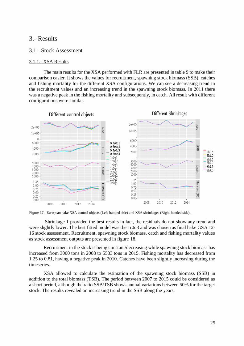
25

3.- Results

3.1.- Stock Assessment

3.1.1.- XSA Results

The main results for the XSA performed with FLR are presented in table 9 to make their

comparison easier. It shows the values for recruitment, spawning stock biomass (SSB), catches

and fishing mortality for the different XSA configurations. We can see a decreasing trend in

the recruitment values and an increasing trend in the spawning stock biomass. In 2011 there

was a negative peak in the fishing mortality and subsequently, in catch. All result with different

configurations were similar.

Shrinkage 1 provided the best results in fact, the residuals do not show any trend and

were slightly lower. The best fitted model was the 1r0q3 and was chosen as final hake GSA 12-

16 stock assessment. Recruitment, spawning stock biomass, catch and fishing mortality values

as stock assessment outputs are presented in figure 18.

Recruitment in the stock is being constant/decreasing while spawning stock biomass has

increased from 3000 tons in 2008 to 5533 tons in 2015. Fishing mortality has decreased from

1.25 to 0.81, having a negative peak in 2010. Catches have been slightly increasing during the

timeseries.

XSA allowed to calculate the estimation of the spawning stock biomass (SSB) in

addition to the total biomass (TSB). The period between 2007 to 2015 could be considered as

a short period, although the ratio SSB/TSB shows annual variations between 50% for the target

stock. The results revealed an increasing trend in the SSB along the years.

Figure 17 - European hake XSA control objects (Left-handed side) and XSA shrinkages (Right-handed side).

26

3.1.1.1.- Diagnostics

The residuals show a decreasing trend but otherwise no pattern (Table 8).

Despite of all the diagnostic analysis were good in all the runs the 1r0q3 was slightly

the best. Retrospective analysis shows good correlation between cohorts and consistent results.

Residuals per age and year of the tuning fleet were relatively low, ranging from -3 to 3 and did

not show any tendency with time (Table 8).

3.1.1.2.- Reference Points

The diagnostics of stock status shows; i) high overfishing and overexploited status

(Fcurrent < F0.1), ii) relative low biomass.

Figure 18 - European hake in GSA 12-16. Estimates of recruitment, SSB, Catch and F for the final run

Figure 19 - European hake in GSA 12 -16. XSA. Diagnostics for the best run for shrk.age=1. Log Residuals of the best XSA configuration analysis (left), retrospective analysis (right).

27

Table 8 - European hake GSA 12-16 XSA reference points

The results of the Y/R analysis (table 8, figure 20) showed that the present rate of

exploitation (equal to 1) is beyond the optimal biological yield for sex combined European hake

stock.

The reference points calculation shows Fcurrent (0.81) > F0.1 (0.117). The ratio Fcurrent/F0.1

is 6.92. It means that the current stock status is overexploited. The survey data timeseries

indicated a relative intermediate biomass of the stock. A reduction of approximately 592% is

necessary to manage the resource to biological safe limits.

For that reason, as agreed with the WGSAD 2015, a reduction of fishing mortality

towards the reference point is advised.

3.1.2.- Deterministic Assessment for All (a4a)

Deterministic a4a stock assessment results were similar to XSA. Due the

introduction of a filter in the F, spawning stock biomass and fishing mortality models the results

are softer. Main results are presented in figure 21. A4a assessment shows a variable but constant

mean recruitment along the timeseries. SSB has been increasing since 2010 to 2014. It is

possible to see a light decreasing in the trend during the last reported year. Catch has been

increasing slightly during the time series. Fishing mortality values are variable during the

timeseries.

Fcurrent 0.81

FMSY 0.180

F0.1 0.117

Fcurrent/F0.1 6.92

Fmax 0.180

Current SSB (tons) 5333.3

33rd percentile SSB (tons) 1759.9

66th percentile SSB (tons) 3519.9

Figure 20 - European Hake GSA 12-16 Summary of the yield per recruit

analysis (Y/R) results.

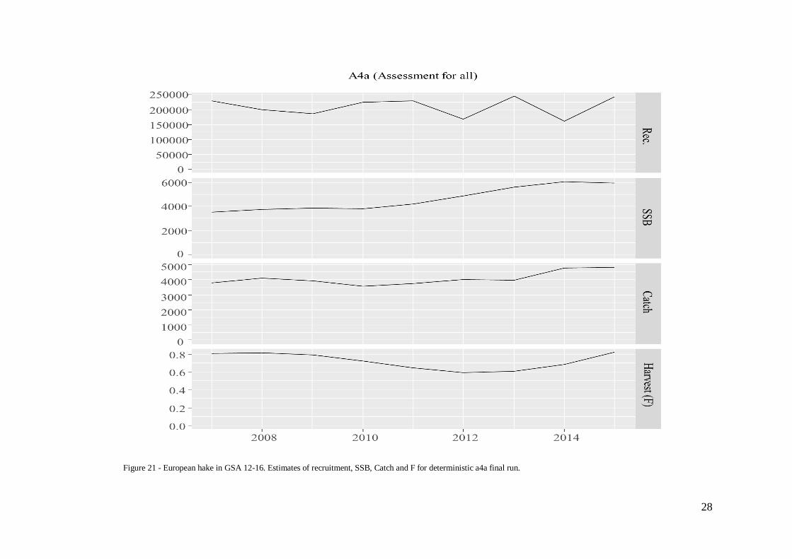
28

Figure 21 - European hake in GSA 12-16. Estimates of recruitment, SSB, Catch and F for deterministic a4a final run.

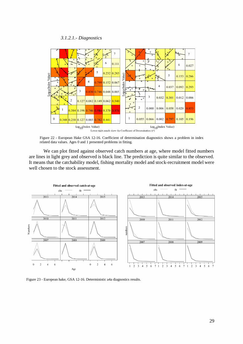
29

3.1.2.1.- Diagnostics

We can plot fitted against observed catch numbers at age, where model fitted numbers

are lines in light grey and observed is black line. The prediction is quite similar to the observed.

It means that the catchability model, fishing mortality model and stock-recruitment model were

well chosen to the stock assessment.

Figure 22 - European Hake GSA 12-16. Coefficient of determination diagnostics shows a problem in index related data values. Ages 0 and 1 presented problems in fitting.

Figure 23 - European hake, GSA 12-16. Deterministic a4a diagnostics results.

30

Quantile plot shows a good residuals fitting, keeping the values between -2 and 2. There

are not strong residuals trend in the survey for all ages.

3.1.2.2.- Reference Points

Reference points shows an overexploited stock status (Fcurrent/F0.1 = 4) with relative high

biomass. The fishing effort that could lead to the fishery towards biological safe limits is

estimated in ¡Error! No se encuentra el origen de la referencia.26. F0.1 could be achieved w

ith a reduction of 300% Fcurrent. Biomass value is relatively high.

Figure 25 - Quantile plot of log residuals diagnostics shows a good fitting level in the stock assessment diagnostics.

Figure 24 - European hake in GSA 12 -16. Bubble plot, Deterministic a4a assessment residuals.

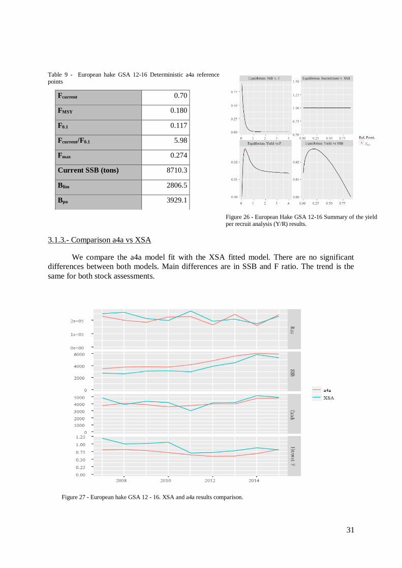
31

Table 9 - European hake GSA 12-16 Deterministic a4a reference points

3.1.3.- Comparison a4a vs XSA

We compare the a4a model fit with the XSA fitted model. There are no significant

differences between both models. Main differences are in SSB and F ratio. The trend is the

same for both stock assessments.

Fcurrent 0.70

FMSY 0.180

F0.1 0.117

Fcurrent/F0.1 5.98

Fmax 0.274

Current SSB (tons) 8710.3

Blim 2806.5

Bpa 3929.1

Figure 26 - European Hake GSA 12-16 Summary of the yield per recruit analysis (Y/R) results.

Figure 27 - European hake GSA 12 - 16. XSA and a4a results comparison.

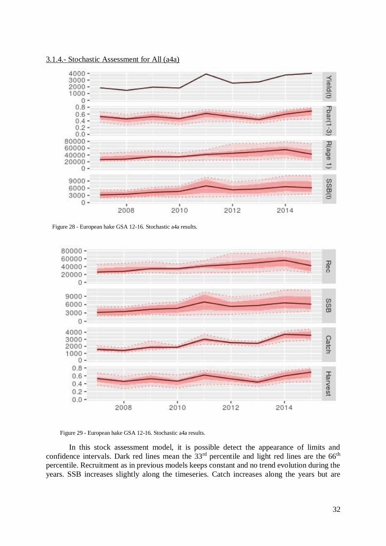
32

3.1.4.- Stochastic Assessment for All (a4a)

In this stock assessment model, it is possible detect the appearance of limits and

confidence intervals. Dark red lines mean the 33rd percentile and light red lines are the 66th

percentile. Recruitment as in previous models keeps constant and no trend evolution during the

years. SSB increases slightly along the timeseries. Catch increases along the years but are

Figure 28 - European hake GSA 12-16. Stochastic a4a results.

Figure 29 - European hake GSA 12-16. Stochastic a4a results.

33

significantly lower comparing with the rest of models. Some data problems are reported in this

section.

Figure 28 shows a yield increasing during the reported years. Fbar (1-3) remained constant

during the timeseries.

3.1.4.1.- Reference points

Reference points calculation detected overexploitation of the target stock

(Fcurrent/F0.1 = 8 – 3.22). The 2 values are due the presence of confidence intervals. Biomass is

relatively high.

Table 10 - European hake GSA 12-16 Stochastic a4a reference points

Fcurrent 0.69246 ± 0.1182

FMSY 0.21307 ± 0.0643

F0.1 0.14407 ± 0.0450

Fcurrent/F0.1 8 – 3.22

Fmax 0.21307 ± 0.0643

Current SSB (tons) 4845.4 ± 1448

Blim 1598.8

Bpa 3197.96

34

3.2.- Short term forecast

3.2.1.- XSA

Table 11 - European Hake in GSA 12-16. XSA. Short term forecast under different F scenarios (3-year average, 2013-2015) weight

at age, maturity at age and F at age. Recruitment (age 0) geomean 2013-2015.

Ffactor Fbar Catch 2015 Catch 2016 Catch 2017

Catch

2018

SSB

2017

SSB

2018

Change SSB

2017-2018(%)

Change Catch

2015-2016(%)

1 0.00 0.00 4959.23 4869.48 0.00 0.00 5089.42 10749.32 111.21 -100.00

2 0.10 0.08 4959.23 4869.48 689.68 1206.67 5089.42 9845.40 93.45 -86.09

3 0.20 0.17 4959.23 4869.48 1322.02 2155.06 5089.42 9025.54 77.34 -73.34

4 0.30 0.25 4959.23 4869.48 1902.27 2893.16 5089.42 8281.53 62.72 -61.64

5 0.40 0.33 4959.23 4869.48 2435.15 3460.47 5089.42 7606.00 49.45 -50.90

6 0.50 0.41 4959.23 4869.48 2924.94 3889.47 5089.42 6992.32 37.39 -41.02

7 0.60 0.50 4959.23 4869.48 3375.50 4206.82 5089.42 6434.53 26.43 -31.94

8 0.70 0.58 4959.23 4869.48 3790.32 4434.42 5089.42 5927.28 16.46 -23.57

9 0.80 0.66 4959.23 4869.48 4172.58 4590.18 5089.42 5465.72 7.39 -15.86

10 0.90 0.75 4959.23 4869.48 4525.12 4688.78 5089.42 5045.52 -0.86 -8.75

11 1.00 0.83 4959.23 4869.48 4850.56 4742.19 5089.42 4662.76 -8.38 -2.19

12 1.10 0.91 4959.23 4869.48 5151.23 4760.19 5089.42 4313.92 -15.24 3.87

13 1.20 0.99 4959.23 4869.48 5429.28 4750.72 5089.42 3995.80 -21.49 9.48

14 1.30 1.08 4959.23 4869.48 5686.64 4720.21 5089.42 3705.55 -27.19 14.67

15 1.40 1.16 4959.23 4869.48 5925.06 4673.88 5089.42 3440.58 -32.40 19.48

16 1.50 1.24 4959.23 4869.48 6146.15 4615.93 5089.42 3198.54 -37.15 23.93

17 1.60 1.33 4959.23 4869.48 6351.36 4549.72 5089.42 2977.32 -41.50 28.07

18 1.70 1.41 4959.23 4869.48 6542.00 4477.95 5089.42 2775.03 -45.47 31.92

19 1.80 1.49 4959.23 4869.48 6719.29 4402.75 5089.42 2589.93 -49.11 35.49

20 1.90 1.57 4959.23 4869.48 6884.30 4325.80 5089.42 2420.47 -52.44 38.82

21 2.00 1.66 4959.23 4869.48 7038.05 4248.41 5089.42 2265.23 -55.49 41.92

22 0.22 0.18 4959.23 4869.48 1426.11 2296.75 5089.42 8891.46 74.70 -71.24

35

Short term projection shows that: i) Fishing a at Fstatus quo (0.81) generates a decreasing

of the catch of approximately 23% from 2017 to 2018 along with an increasing of the spawning

stock biomass of the 16% from 2017 to 2018; ii) fishing at F0.1 (0.22) generates a decrease of

the catch of the 71% from 2017 to 2018 and an increase of the spawning stock biomass of 74%

from 2017 to 2018.

Different and alternative scenarios are shown at Table 12.

Figure 30 - XSA short term forecast.

36

3.2.2.- Deterministic a4a

Deterministic a4a short-term forecasting demonstrate the similarity in the results

between both models. Fishing at Fstatus quo level will generate a change in the SSB of 9%. Catches

could increase 26% of the total catch value since 2015 – 2016. Fishing at F0.1 level could

increase the SSB up to 52%, and catches could be reduced 55%.

Different and alternative scenarios are at Table 12.

Table 12 - European Hake in GSA 12-16. Deterministic a4a short term forecast under different F scenarios (3-year average, 2013-2015) weight at age, maturity at age and F at age. Recruitment (age 0) geomean 2013-2015

Ffactor Fbar Catch 2015 Catch 2016 Catch 2017

Catch

2018

SSB

2017

SSB

2018

Change SSB

2017-2018(%)

Change Catch

2015-2016(%)

1 0 0.00 5144.41 6164.13 0.00 0.00 12081.83 21388.62 77.03 -100.00

2 0.1 0.05 5144.41 6164.13 806.80 1207.56 12081.83 20354.36 68.47 -84.32

3 0.2 0.09 5144.41 6164.13 1574.12 2254.61 12081.83 19377.28 60.38 -69.40

4 0.3 0.14 5144.41 6164.13 2304.15 3160.35 12081.83 18453.97 52.74 -55.21

5 0.4 0.18 5144.41 6164.13 2998.94 3941.73 12081.83 17581.26 45.52 -41.70

6 0.5 0.23 5144.41 6164.13 3660.43 4613.70 12081.83 16756.16 38.69 -28.85

7 0.6 0.28 5144.41 6164.13 4290.45 5189.45 12081.83 15975.87 32.23 -16.60

8 0.7 0.32 5144.41 6164.13 4890.70 5680.59 12081.83 15237.76 26.12 -4.93

9 0.8 0.37 5144.41 6164.13 5462.79 6097.40 12081.83 14539.36 20.34 6.19

10 0.9 0.41 5144.41 6164.13 6008.26 6448.93 12081.83 13878.36 14.87 16.79

11 1 0.46 5144.41 6164.13 6528.52 6743.16 12081.83 13252.57 9.69 26.90

12 1.1 0.51 5144.41 6164.13 7024.91 6987.15 12081.83 12659.96 4.79 36.55

13 1.2 0.55 5144.41 6164.13 7498.72 7187.11 12081.83 12098.62 0.14 45.76

14 1.3 0.60 5144.41 6164.13 7951.14 7348.53 12081.83 11566.73 -4.26 54.56

15 1.4 0.64 5144.41 6164.13 8383.28 7476.24 12081.83 11062.61 -8.44 62.96

16 1.5 0.69 5144.41 6164.13 8796.21 7574.52 12081.83 10584.67 -12.39 70.99

17 1.6 0.74 5144.41 6164.13 9190.94 7647.13 12081.83 10131.42 -16.14 78.66

18 1.7 0.78 5144.41 6164.13 9568.40 7697.40 12081.83 9701.46 -19.70 86.00

19 1.8 0.83 5144.41 6164.13 9929.48 7728.24 12081.83 9293.45 -23.08 93.01

20 1.9 0.87 5144.41 6164.13 10275.02 7742.25 12081.83 8906.18 -26.28 99.73

21 2 0.92 5144.41 6164.13 10605.82 7741.69 12081.83 8538.47 -29.33 106.16

22 0.29 0.14 5144.41 6164.13 2293.20 3147.41 12081.83 18467.77 52.86 -55.42

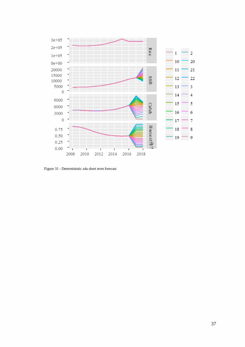
37

Figure 31 - Deterministic a4a short term forecast

38

3.3.- Medium-Long term forecast and assessment of management scenarios

3.3.1.- XSA

Management strategy evaluation for extended survivor analysis stock assessment has

shown that in Status Quo scenario no significant change in stock status happened. Recruitment,

spawning stock biomass, catch and fishing mortality remained constant during projected years.

The possibility of dropping below Blim was equal to 0.

During the achievement of F0.1reference point choosing F0.1 as a proxy of Fmsy showed

a high and fast increasing of the spawning stock biomass, generating proportional increasing of

the catch values along the projected years. Recruitment remained constant and fishing mortality

also at F0.1 level (0.22). The possibility of dropping below Blim was equal to 0.

In the reduction of 50% of current F, the simulations generated an increasing of the

spawning stock biomass and catch. Recruitment was constant and F at level of 0.4 too. This

measure generates an important stock recovery effect. The possibility of dropping below B lim

was equal to 0.

Increasing the previous scenario to a 70% F reduction, the stock recovery capacity was

increased comparing with the previous scenario. The recovery time (slope of the graph) and

maximum level of SSB increased significantly. The possibility of dropping below Blim was

equal to 0.

Most restrictive scenario (90% F reduction) generated the expected effect. Fast increase

and maximum level of the SSB during time series was noticed. Recruitment, as in the previous

scenarios remained constant. The possibility of dropping below Blim wa equal to 0.

3.3.2.- Deterministic a4a

Assessing Status Quo scenario, recruitment, spawning stock biomass, catches and

fishing mortality remained constant during all projected years. No significant changes took

place in the stock status. The possibility of dropping below Blim is equal to 0.

During F0.1 scenario, recruitment remained constant and harvest decreased until F0.1

level and kept constant during the timeseries (from 2016 to 2035 F is equal to 0.11). In the

scenario, there were significant changes in the SSB and in catches. Both variables increased

significantly. The possibility of dropping below Blim is equal to 0.

50% F reduction scenario showed that recruitment was kept constant while SSB and

catches increased significantly with the same slope for both variables. There was no possibility

of dropping below Blim.

70% F reduction, as in the previous model, recruitment remained constant and the rest

of variables (excepting fishing mortality) increased to 10000 tons and 6000 tons for spawning

stock biomass and catches respectively. The possibility of dropping below Blim was equal to

0.

In 90% F reduction scenario changes were more significant, spawning stock biomass

increased to 100000 tons and catches to 7500 tons. Recruitment, as in the previous scenarios

remained constant. No possibility of dropping below Blim existed in this scenario.

39

3.3.3.- Stochastic a4a

Management strategy evaluation showed higher uncertainty boundaries in

forecasting.

During scenario 1, Status Quo, no significant changes occurred in stock values. SSB

decreased non-significantly. Catch value remained constant along the timeseries. No significant

variations took place in this scenario. There existed a possibility of dropping below Blim in this

scenario.

In F0.1 scenario, F decreased until the F0.1 value. Catches, after a big peak, increased

significantly. Also spawning stock biomass increased overcoming historical maximums. As in

the rest of scenarios, recruitment remained constant. No possibility of dropping below Blim

existed in this scenario.

50% F reduction scenario showed a decrease in catches significantly until 2020, when

catches slightly increased. A high reduction on fishing mortality took place arriving to historical

minimums. A low increase in spawning stock biomass happened in this scenario. No possibility

of dropping below Blim existed in this scenario.

Along 70% F reduction SSB was increased. Catch, after a low peak was recovered

bellow historical minimum. As in the rest of scenarios, recruitment remained constant. The

possibility of dropping below Blim in this scenario existed.

During 90% F reduction scenario, the spawning stock biomass increased significantly.

Catches are approximately 30% of the historical value and F remained in historical minimums.

Recruitment still constant. Low possibility of dropping below Blim exists.

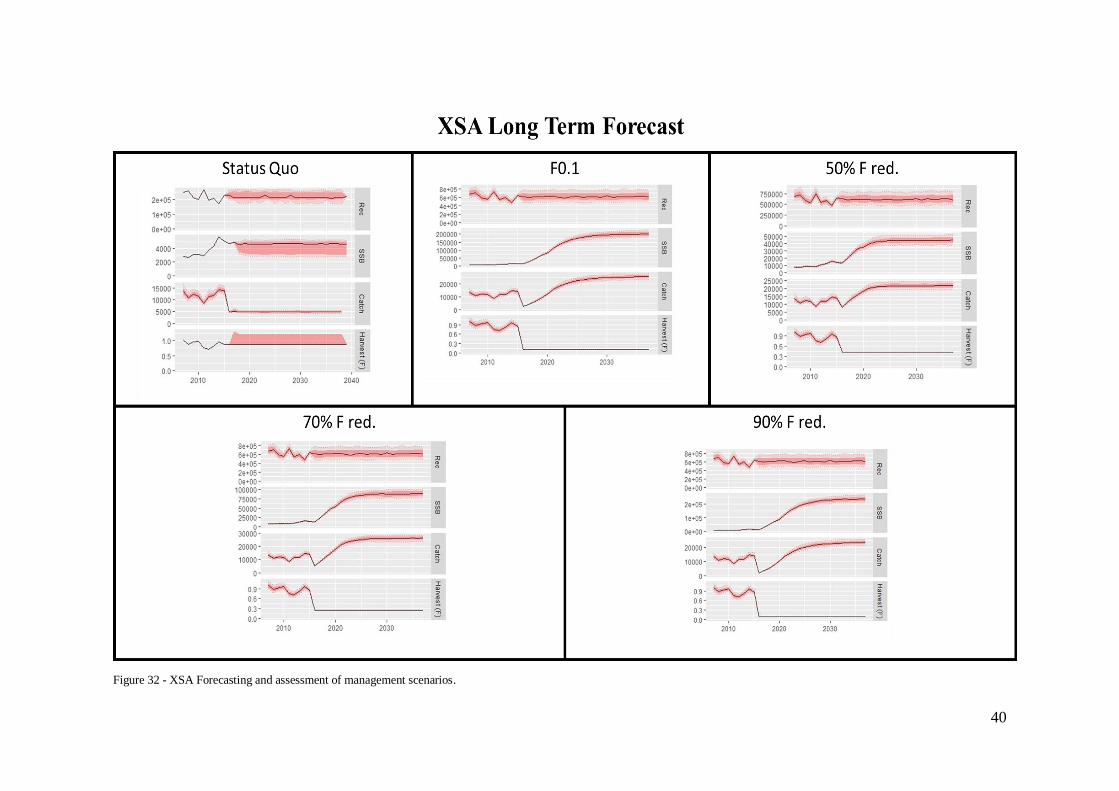
40

Figure 32 - XSA Forecasting and assessment of management scenarios.

41

Figure 33 - Deterministic a4a forecasting and assessment of management scenarios.

42

Figure 34 - Stochastic a4a forecasting and assessment of management scenarios.

43

4.- Discussion

4.1.- Stock assessment results and advice

As during the 2016 working group on stock assessment (GFCM WGSAD, 2016),

XSA European hake stock assessment showed an overexploited status of the resource

(Fcurr > F0.1) with a relative intermediate biomass in GSAs 12 -16. Despite of diagnosis of

the stock status is the same for the three models used during the research (XSA,

deterministic a4a and stochastic a4a), the values of Fcurr and SSBcurr. are quite different.

The reason to explain the differences in some stock assessment outputs could be the

differences between how each model computes catchability and the way to estimate the

biomass. XSA has problems to incorporate selectivity patterns and uncatchable

individuals for the fishing gear due accessibility. a4a estimates the individuals impossible

to catch by the fishing gear. The reference points estimated by all models were similar

with slight differences.

In developed stock assessment achieving F0.1 implies a reduction in current fishing

mortality of 80, 70 and 65 percent in XSA, deterministic a4a and stochastic a4a

respectively. European hake in GSAs 12-16 is a shared stock by Italy, Malta and Tunisia.

For that reason, Fcurr should be reduced considering the contribution to the catch of each

fleet exploiting the stock.

Concerning to the used models, XSA and a4a are methods based on pseudocohorts

analysis. Those methods assume of the equilibrium of the stocks and its exploitation and

the constancy of the annual recruitment (Aldebert & Recasens 1996). Historically, along

the studied timeseries, the conditions of the exploitation of hake stock in GSAs 12 – 16

remained quite steady (Fiorentino et al., 2003). However, constant recruitment trend has

been observed without peaks along the timeseries but with important large landings of

group 0 fish. Pseudocohorts based on 8 years and constant recruitment trend are enough

to obtain robust results. Some of the Extended Survival Analysis limitations are: i)

Stochasticity in the model for a proper description of the stocks; ii) Incapability to

separate the effects of different fleets and therefore simulate the effects of different

management measures on different fleets; iii) Impossibility to incorporate spatial aspects

when assessing management scenarios; iv) Impossibility to incorporate species

interactions, as well as interactions with the environment; v) Impossible to deal with

bioeconomical information to test potential effects of alternative management scenarios

on the fishery.

Through the calculation of stock assessment diagnostics, some problems in some

ages and during some years were noticed. Specially in the catch-at-age matrix. Age 0

probably is not well represented. The possible cause are the difficulties to sample discards

in the Mediterranean and Black sea fisheries. It makes difficult to simulate the effects of

an improvement in selectivity and other management scenarios. Also, the data series used

to do the stock assessment are enough, but ideally, more years are necessary to improve

the stock assessement quality. Also, relating to growth and natural mortality parameters,

there are existing gaps on the calculation of those parameters. It is necessary continue

with data acquisition inside “GFCM data collection reference framework” to increase the

data acquisition, data quality and obtain better timeseries. GFCM data collection

reference framework “is the first comprehensive GFCM framework for the collection and

44

submission of fisheries-related data in the GFCM area (Mediterranean and Black Sea). It

is the result of a series of coordinated actions focused on fisheries data collection which

were launched in 2013 under the umbrella of GFCM Scientific Advisory Committee

(SAC) and considering the inputs of the GFCM Working Group on the Black Sea

(WGBS) (GFCM DCRF, 2016)”. This tool indicates how to obtain different kind of data.

Some of the referred data are: i) National fisheries; ii) Catch; iii) Incidental catch of

vulnerable species; iv) Fleet; v) Effort; vi) Socioeconomics; vii) Biological information.

It also indicates the “common practices in data collection”. These data are of paramount

importance for the work of the GFCM to support to the decision-making process based

on sound scientific advice from its subsidiary bodies (GFCM DCRF, 2016). As agreed

with GFCM WGSAD, it is recommended to stablish a European hake tagging project to

obtain essential data on growth, natural mortality, migration patterns and connectivity.

4.2.- Uncertainty in Stock Assessment: Stochastic a4a

Measurement (observation) uncertainty occurs in any process of collecting field

data, and might be due to crude devices or mistakes during measurement. These two

forms of uncertainty combine to form parameter uncertainty. Structural uncertainty (also

called ‘model uncertainty’) has received increased attention in modelling natural

resources and represents our lack of understanding of the dynamics of the system.

Representing structural uncertainty is generally difficult because a model representing the

real system according to our perceptions is only one possible way in which the system

could function. Implementation uncertainty surrounds the translation of policy into

practice, and has been poorly covered in the literature on natural resources because its

causes lie within social science; one example is institutional inertia, another is non-

compliance with rules. MSE models the entire resource management system rather than

just the resource stock dynamics. Hence, it can incorporate all these types of uncertainty

and quantify their relative importance (Bunnefeld et al., 2011).

Stochastic assessment for all seems the best alternative to replace extended

survival analysis during the stock assessment process. This work agrees with the WGSAD

(GFCM WGSAD, 2016) and demonstrates that statistical-catch-at-age (SCAA) methods

as a4a allowed to a better understanding of the fluctuations and dynamics of the stocks

over the years. Those methods should be promoted in the assessment and management

bodies in the Mediterranean region. Nevertheless, there are technical difficulties in

shifting towards the use of such complex models. It is necessary increase capacity-

building initiatives as, for example, trainings (GFCM WGSAD, 2016). However, during

the realization of the research, we notified that a4a is an easier to use tool and to

understand by the scientific non-specialized community in stock assessment.

Although uncertainty could be introduced in other ways using the same stock

assessment model (for example, Markov Chain Monte Carlo simulation, bootstrapping,

etc) (Ralston et al. 2011) those just represent the structural uncertainty1. Current

investigation proposes include regularly other existing errors during the stock assessment

process. As, for example, uncertainty in growth parameters or in natural mortality

parameters. The aim would be obtaining better and more precise representations of the

system reality in which ones’ uncertainty had been considered. Other authors as Deroba 1 Probability of the occurrence of an unanticipated event due to the configuration of a system.

45

et al., 2015 and Williams, 1997 proposed the same to increase the quality of the advice.

Main problem of the deterministic approach (just one value without uncertainty) is that

sometimes, the manager, to carry on the management measure it is built over the best

simulation scenario (Deroba et al., 2015) and not in extreme situations.

Nowadays, statistical-catch-at-age models as a4a or SAM and integrated analysis

like SS3 or GADGET could allow us to estimate of reliable biomass reference points in

stocks with robust stock-recruitment relationship estimations (GFCM WGSAD, 2016).

Those biomass reference points are key actors for the establishment of a harvest

control rule (HCR). Harvest strategies and decision rules provide a formal and more

consistent approach to the management decision making process by defining what actions

will occur based on the current or likely future performance of a fishery in relation to one

or more of its operational objectives (FAO - EAFnet). The establishment of HCR will

help to develop political decisions to explicitly reflect long-term preferences (Kvamsdal,

et al., 2016) and definitively to better management of the resource.

4.3.- Assessment of Management Scenarios

Management processes (management strategy evaluation) is done to test and

recommend management measures and assessment methods which take care about

structural uncertainty and observed parameters during data collection process.

Bioeconomical assessment should be done for the realization of a full MSE. For this

reason, during the current investigation an assessment of management scenarios was

done, not a full management strategy evaluation.

Within fisheries assessment and management, the MSE approach is the most

closely related to the development and evaluation of management procedures. The key

ingredients to develop a MSE are: i) Specifying key management objectives; ii) develop

quantifiable performance measures for each objective; iii) identify alternative

management strategies or decision options; iv) evaluate the performance of each strategy;

v) communicate the results to decision makers (Smith et al., 1999). Due the absence of

time during the research, some of those parts were not assessed. It is the cause why a full

MSE approach was not completed.

The management simulations depend on the stock assessment models adopted and

are therefore subject to the same limitations and uncertainties as these models. Stock

assessment uncertainties were in general well described by the WGSAs, which formulate

recommendations every year to improve the quality of the stock assessment models. The

quality of the input data and the duration of the time series were crucial for the analysis

being necessary an extra effort to improve the information used in stock assessement and

therefore ensure the best quality advice.

MSE, in common with adaptive management more generally, has four major

advantages over standard approaches to providing management advice. Firstly, it allows

experimentation with a range of possible management procedures under a range of

circumstances. Real-world experimentation is highly desirable to disentangle the drivers

of a system, but is difficult to pursue for most natural resources because of the dependence

of individuals and firms on resources for their livelihoods and the spatial extent of the

systems. In conservation, real-world experimentation poses ethical dilemmas: local

people often depend on ecosystem services for subsistence, whereas endangered species

46

may face extinction. Secondly, stakeholders can be directly involved in the development

of the management scenarios and the evaluation of the metrics by which the performance

of different management options is assessed. A key feature of the MSE approach is that

an optimal strategy or solution is not pursued, but instead policies are sought that are

feasible, robust to uncertainty, and which provide adequate management performance

with respect to multiple criteria. This allows for more transparency in the management

process and promotes the acceptance and support of stakeholders. Thirdly, MSE enables

researchers and managers to examine the implications of various forms of uncertainty

(including process, measurement and structural uncertainty) on the performance of

different management options. Fourthly, MSE carries out prospective (rather than

retrospective) evaluations of the performance of different management procedures under

a range of circumstances. By comparing the performance of a range of alternative

strategies under plausible scenarios upfront, the response of the system can be compared

with the desired goals and evaluated in advance of implementation.

Limitations of MSE Management of natural resources is plagued by uncertainty

and feedbacks between the dynamics of resources and users. Although MSE goes some

way towards addressing these difficulties, it has been criticized for: (i) having a longer

development time (and thus increased costs) than traditional methods such as reference-

based off-take rules; (ii) an upfront MSE can provide an overly rigid framework without

room for decision-makers to change management in an adaptive way; and (iii) poor data

inputs (e.g., gaps in monitoring or extremely low estimates of uncertainty) affect the

performance of MSE, which needs to be recognized and explored within the MSE

process. These criticisms point to the need for an iterative process of monitoring, learning

and adaptation, which is entirely in keeping with the MSE approach if practitioners are

prepared to engage with the issues being raised.

Along the investigation, bioeconomic analysis were not performed except for an

evaluation of variations in catch levels in response to the implementation of different

management scenarios. It could be a continuation of the present work evaluating and

assessing the bioeconomical implications of the proposed management scenarios.

MEFISTO could be the tool to accomplish the objective.

4.4.- Mediterranean Sea: Status and future

Overall current situation of the Mediterranean stocks is bad (85% of overexploited

stocks) (GFCM, 2016). However, there are indicators that countries are about the urgency

of taking measures and actions to improve the quality of advice and the management of

stocks. For example, i) the percentage of assessed landings has nearly doubled in recent

years, rising from 20 percent in 2013 to 45 percent in 2015 (GFCM, 2016). It is a good

reference point to assess the improvement of the scientific advice.

Also, there are important initiatives on way that could be good guidelines to

progress and improve the scientific advice. Some initiatives, in addition of GFCM Mid-

Term strategy, for the Mediterranean Sea are: i) The use of fleet-based assessment models

as operational models for the assessment of management scenarios towards a more

comprehensive Management Strategy Evaluation (MSE) framework including

uncertainty and evaluation of socioeconomic impact (GFCM, SAC, 2016); ii) The

improvement of stock biological information; iii) The creation of a management plan for

small pelagic fisheries management in Adriatic Sea; iv) The increase of the technical and

47

operational measures to facilitate the provision of advice for the GFCM; v) The creation

of areas of discussion at subregional level to create discussions and deliberations on

fisheries management in their subregion and vi) The development of training courses.

Within this context the improvement on coverage and the precision of the advice

should facilitate the adoption of more and better management measures to improve the

state of Mediterranean and Black Sea fisheries.

49

5.- Conclusion

The obtained results during this master thesis are consistent with previous

scientific advice given to the Central Mediterranean subregion for European hake.

• European hake in GSA 12-16 stock assessment has shown an

overexploited status of the resource being necessary the adoption of measures to

reduce the fishing mortality and guarantee the sustainability of the resource.

Nevertheless, the short term and long-term forecast demonstrates us a steady

situation of the stock, being possible to reverse the situation of the resource.

• Simulations using both XSA and deterministic a4a models were generally

coherent. All the presented scenarios in deterministic models followed the same

stock dynamics trends. Using stochastic a4a stock assessment methods increases

the uncertainty in the forecast of management scenarios due the introduction of

structural and observation uncertainty.

• Comparison between models show us the capability of a4a to replace XSA

methods to assess the stock status of the Mediterranean and Black Sea living

resources due the similarity between both results. It is necessary to include the

uncertainty in the stock assessment parameters to do a development of the

statistical stock assessment able to predict the future behaviour of the stock.

Uncertainty in stock assessment is key to improve the assessment and

management of Mediterranean marine resources. It will help to achieve biomass

reference points and, at the end, to build harvest control rules in the GFCM area.

51

6.- Future steps

Technical activities towards the assessment of management measures could be

carried out during further investigations:

• A similar experiment could be carried on comparing the similarities and

dissimilarities between both technics (XSA and a4a) in different GSA’s and

between different kind of fisheries, for example, small pelagic fisheries and to

species outside the GFCM study area.

• Trawlers are the main fishing gear who targets European hake, nevertheless,

other fishing sectors targets also European hake. An interesting experiment

could be to introduce new fishing sectors for the stock assessment of this

species.

• Different management scenarios have been tested during the current research.

However, no spatial aspects have been assessed. A useful activity could be to

incorporate spatial aspects, as for example, the closure of spawning areas as

management scenarios.

• Introduction of interaction between species and ecosystem may be useful to

achieve better assessment and management results for further investigations.

• An important activity for the application of the methods used during the thesis

is the assessment of bioeconomic implications of the simulated scenarios

results. Could be useful to test the potential effects of alternative management

scenarios on the fishery. Some models as MEFISTO or BEMTOOLS are

valuable to achieve this objective.

• Elaborate a harvest control rule for the hake in the Strait of Sicily.

55

Chapter 2

Calculation of Reference Points in

Decreasing Trend Populations

57

1.- Introduction

The Earth’s climate has warmed by approximately 0.6ºC over the past 100 years

(Walther et al., 2002). Resolve the effects of climate change in fish populations is

complicated. It is due climate change affects a multitude of environmental factors that

may affect various processes at different levels of biological organization (Harley et al.,

2006). It may be argued that it will be impossible to detect generalities in the response of

fish populations to climate change, because the number of influential factors is too large

and individual species may differ too widely in their response (Lehodey et al., 2006).

Effects of climate change are expected to differ in magnitude and direction of among

geographic areas (IPCC - Intergovernmental Panel on Climate Change, 2007). Impacts in

marine areas remain uncertain. Climate change will affect a range of abiotic factors that

are tightly linked to the production and distribution of fish populations. These biotic

changes will differ between the open ocean, shelf seas and coastal waters (Walther et al.

2002).

In fish, one of the potential impacts of temperature increasing is over the eggs.

The temperature increasing has a highly significant effect of decreasing egg incubation

time, generating a high increasing of the daily mortality rate of pelagic fish eggs and

larvae (Pepin 1991). For example, changes in the physical environment already impacted

over cod (Gadus morhua) recruitment in the North Sea (Beaugrand 2003). The

temperature increasing also produces impacts on primary production and unbalances the

whole marine food chain (Brunel & Boucher 2007). Changes in catches of North Sea

horse mackerel (Trachurus trachurus) (Reid 2001) and Atlantic salmon (Salmo salar)

(Beaugrand & Reid 2003) were related to changes in the physical environment and in the

plankton community (Brunel & Boucher 2007).

Global marine fisheries are underperforming because of overfishing, pollution and

other anthropogenic causes. These changes are expected to affect the productivity of

marine fisheries leading to losses in revenues, earnings to companies and household

incomes (Da Rocha et al., 2014). Recent commitments to adopting an ecosystem

approach to fisheries may influence the fact of the reassessment of management targets

fitness considering the current scenario with the conservation targets (Worm 2009)

From the management point of view, using a static reference point in a dynamic

situation could generate an overestimation of the current stock status. This fact produces

also differences in the reference points and causes negative effects in the fisheries

management decreasing fishermen’s and stockholder’s profits.

Summarizing, the growth rate of a fishery resource is subject to changing

conditions under global warming. Thus, the population can never be in equilibrium until

the ocean temperature stabilises. Technically, global warming alters the steady-state

situation. The process is called transitional dynamics (Da Rocha et al., 2014).

This study develops population dynamics of sardine (Sardina pilchardus,

Walbaum, 1792) in regions VIIIc and IXa by evaluating the consequences for stock

assessment and management. The research also compares the differences between the

management measures and reference points considering stochastic or deterministic

recruitment of the target population. Finally, the study checks the robustness changes of

both methods to reduce the uncertainty during the process.

58

The contribution of this work is to show the benefits of include the population

trends into harvest control rules even when it is not possible to estimate the recruitment

with perfect accuracy due the existing uncertainty in the stock-recruitment relationship

(Ludwig & Walters 1981). The gains from adding the recruitment trend into the

management process depends on the accuracy of the estimates. Also, the benefit depends

of stock biology.

These results have direct implications for policy making. First, we show that using

a HCRs that ignore population trends increases the difficulties to achieve the target point,

the stock volatility and underestimates the risk status of the stocks. Second, the necessity

of apply a most precautionary approach to avoid the negative implications to the fishery

and achieve the highest economic benefit.

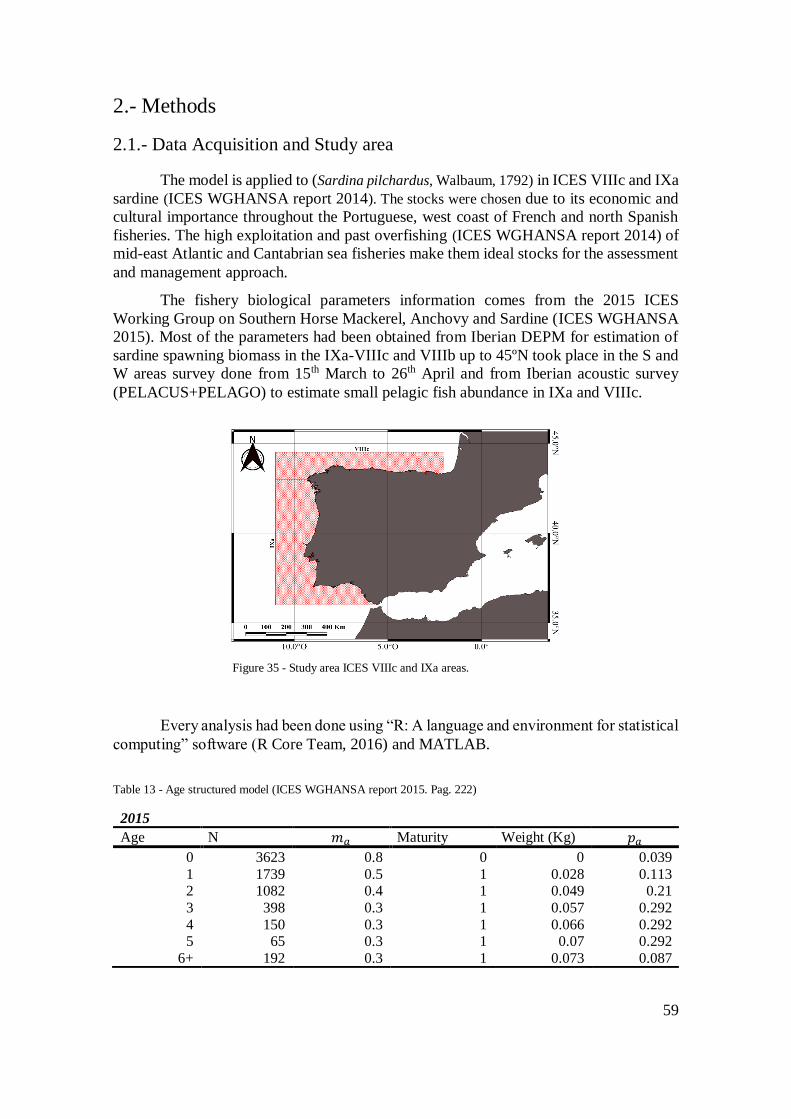
59

2.- Methods

2.1.- Data Acquisition and Study area

The model is applied to (Sardina pilchardus, Walbaum, 1792) in ICES VIIIc and IXa

sardine (ICES WGHANSA report 2014). The stocks were chosen due to its economic and

cultural importance throughout the Portuguese, west coast of French and north Spanish

fisheries. The high exploitation and past overfishing (ICES WGHANSA report 2014) of

mid-east Atlantic and Cantabrian sea fisheries make them ideal stocks for the assessment

and management approach.

The fishery biological parameters information comes from the 2015 ICES

Working Group on Southern Horse Mackerel, Anchovy and Sardine (ICES WGHANSA

2015). Most of the parameters had been obtained from Iberian DEPM for estimation of

sardine spawning biomass in the IXa-VIIIc and VIIIb up to 45ºN took place in the S and

W areas survey done from 15th March to 26th April and from Iberian acoustic survey

(PELACUS+PELAGO) to estimate small pelagic fish abundance in IXa and VIIIc.

Every analysis had been done using “R: A language and environment for statistical

computing” software (R Core Team, 2016) and MATLAB.

Table 13 - Age structured model (ICES WGHANSA report 2015. Pag. 222)

2015

Age N 𝑚𝑎 Maturity Weight (Kg) 𝑝𝑎

0 3623 0.8 0 0 0.039

1 1739 0.5 1 0.028 0.113 2 1082 0.4 1 0.049 0.21

3 398 0.3 1 0.057 0.292

4 150 0.3 1 0.066 0.292 5 65 0.3 1 0.07 0.292

6+ 192 0.3 1 0.073 0.087

Figure 35 - Study area ICES VIIIc and IXa areas.

60

2.2.- Stock Dynamics

A useful simplification of the biological structure of a fishery is to consider a

model with only two ages: Juveniles and adults (Da-Rocha & Mato-Amboage 2016). This

simplified system allows to obtain analytical conclusions to be drawn about the

relationship between the risk of the stock dropping below the limit reference point and

the target reference point.

For the simplification, a stochastic version of Hannesson (Hannesson 1975)

fishery based on Beverton and Holt model with two age classes: Juveniles and adults. Nt,1

and N t,2 are the population of juveniles and adults (respectively) in period t. Each year, t,

a stochastic exogenous number of juvenile fish are born.

𝑁𝑡,1 = exp (𝑍𝑡)

Where 𝑍𝑡 follows an autoregressive (AR) process:

𝑍𝑡+1 = 𝜌𝑍𝑡 + 𝜀𝑡+1

With zero mean, 𝐸𝜀𝑡+1 and variance 𝜎𝑧. The relationship between the number of

recruits today and tomorrow is determined by the parameter 𝜌. Due the unknown

relationship stock-recruitment we assume that the number of juveniles is independent of

the system spawning stock biomass. In that way, the uncertainty in the process is added

simulating a stochastic recruitment.

Additionally, it is assumed that only some of the juveniles survive to become

adults in the next period. The dynamics of the second age group are:

𝑁𝑡+1,2 = 𝑁𝑡,1𝑒−𝑝𝐹𝑡−𝑚

Where m is the natural mortality rate and 𝑝 is the selectivity parameter. The

selectivity parameter indicates how the fishing effort affects the fishing mortality of the

juveniles.

During the 2-age model example 𝑝 is unnecessary, without loss of generality we

normalize 𝑝 = 1.

To simplify the example, the variables can be changed to define the dynamics in

logarithm terms. The stock dynamics become:

Figure 36 - System dynamics

61

log 𝑁1 = 𝑧

And

log 𝑁2 = 𝑥

The population could be represented as:

Time (t)

Age classes 𝑡 𝑡 + 1 𝑡 + 2 𝑡 + 3

Log juveniles z 𝑧𝑡

Log adults x 𝑧𝑡 − 𝐹𝑡 − 𝑚

Finally, the total biomass of the fishery can be defined as:

𝐵𝑡 = 𝑙𝑜𝑔 𝑁𝑡,2

The expression implies that a non-constant fraction of adults are spawners and

that spawning stock biomass (SSB) is an increasing function of the number of adults in

the population.

2.3.- Recruitment Analysis

The trend in the population was analysed using a simple linear regression

(PennState 1.1, 2017). The analysis allowed us to summarize the relationship between the

number of recruits and the sampled years (Chatterje & Hadi, 2006). Dickey – Fuller test

(Dickey & Fuller 1979) was used to test if the unit root is present in an autoregressive

model.

{ 𝑯𝟎 = 𝑼𝒏𝒊𝒕 𝑹𝒐𝒐𝒕 𝒊𝒔 𝒑𝒓𝒆𝒔𝒆𝒏𝒕. 𝑻𝒉𝒆 𝒎𝒐𝒅𝒆𝒍 𝒊𝒔 𝒂𝒖𝒕𝒐𝒓𝒆𝒈𝒓𝒆𝒔𝒔𝒊𝒗𝒆

𝑯𝟏 = 𝑼𝒏𝒊𝒕 𝑹𝒐𝒐𝒕 𝒊𝒔 𝒏𝒐𝒕 𝒑𝒓𝒆𝒔𝒆𝒏𝒕. 𝑻𝒉𝒆 𝒎𝒐𝒅𝒆𝒍 𝒊𝒔 𝒔𝒕𝒂𝒕𝒊𝒐𝒏𝒂𝒓𝒚

To calculate the trend along the time series a Hodrick and Prescott filter (Hodrick

& Prescott et al., 1980) was used. This filter allows us to delete the seasonal, irregular

and trend components to analyse only the cyclical component. Normal distribution of

recruitment timeseries was tested. Logarithm transformation was done in the recruitment

series data to fit the data to the normal distribution and apply the filter. Hodrick and

Prescott filter allowed us to convert the time series from autoregressive to stationary.

62

Main problem of decreasing recruitment trend series is related with the manager

target to minimize the distance between current reference points value and target

reference points value.

2.4.- Fishery management: The role of λ parameter and effects of different 𝛽

over the regulator

The current fishery is managed to achieve an exogenous target reference point (for

example Bmsy and the corresponding Fmsy, B0.1 and F0.1 or any other exogenous target that

represents the manager objectives).

The manager’s objective is to reduce the distance between the current fishing

mortality (Fcurr) and the current system biomass (Bcurr) to the target reference point (Btar

and Ftar), subject to the stock dynamics. In the system, the expectation term is associated

to with the stochastic recruitment process. λ parameter weights the importance of reaching

the objective and determines the strategy (importance of biomass vs effort oriented

objectives). λ value determines the slope of the harvest control rule.

∆𝐹𝑡

∆𝐵𝑡= 𝛽 ∗ λ

Figure 37 - Hodrick and Prescott filter residuals.

Figure 38 - Different kinds of decision rules as a function of the weight parameter λ in the managers objective function.

63

λ = 0 → Constant Effort: The HCR reproduces a constant fishing mortality rule.

λ > 0 → Biological based catch: The HCR reproduces a biomass-based rule.

λ < 0 → Constant catch: The HCR generates a negative relationship between

fishing and biomass, like a constant catch rule.

λ = ∞ → Constant escapement: The HCR reproduces a constant or fixed

escapement rule

The target can be plotted on a 2D graph (Figure 39). It allows to choose the desired

gap between the stock status and the target. This gap is given by the weight that the

manager has on reaching the effort reference point relative to the biomass target, thus

determining whether the fishery is to be managed by effort-focused control rules or

biomass control rules.

The profits of the fishery for any period t are given by the difference between

revenues and fishing costs. For the shake of simplicity, prices are assumed to be constant

over time and total cost to be a convex function (Da Rocha. & Gutierrez 2011).

Note that πt can be interpreted in several ways from the economic point of view

(Da Rocha & Gutierrez 2011). For instance, cost zero (πt) represents the discounted

revenues of the fishery. Alternatively, if the price is one and the cost is zero, represents

πt the discounted yield of the fishery (Da Rocha & Gutierrez 2011).

The objective of the fishery manager is to find the fishing mortality that maximises

the present value of the future profits of the fishery. Formally, the present of future profits

is given by:

𝐽 = ∑ 𝛽𝑡 𝜋𝑡

∞

𝑡=0

The parameter 𝛽 𝜖 [0,1] is the discount factor which represents how much the

manager is willing to pay to trade-off the value of fishing today against the benefits of

increased profits in the future, measured by higher biomass and recruitment (Da Rocha,

et al., 2013). Considering 𝛽 = 1 implies that managers care about future changes as much

Figure 39 - Different strategies to achieve the target comparison.

64

as if they occurred during the current year. By contrast, 𝛽 = 0 implies not caring about

the future at all (Da Rocha et al., 2014).

Therefore, the objective of the fishery managers should be to find the fishing rate

trajectory that maximises the present value of the fishery, 𝐽, considering that the spawning

stock biomass is always greater than the precautionary level, SSBpa. Formally this is a

maximization problem.

Summarizing, the HCR for stochastic age-structured models can be defined as the

optimal feedback policy that minimizes the weighted sum of squares between the stock

assessment outputs and a given “biological reference point”.

max𝐹𝑡.𝐵𝑡+1

𝐸0 ∑ −𝛽𝑡{(𝐹𝑡 − 𝐹𝑡𝑎𝑟)2 +

∞

𝑡=0

λ(𝐵𝑡 − 𝐵𝑡𝑎𝑟)2}

𝑠. 𝑡. {𝐵𝑡+1 = 𝑧𝑡 − 𝐹𝑡 − 𝑚𝑧𝑡+1 = 𝜌𝑧𝑡 + 𝜀𝑡+1

The state variables in this problem are 𝑧𝑡 = log (𝑁1,𝑡) and 𝐵𝑡 = log (𝑁2,𝑡), and 𝐹𝑡

is the control variable.

The objective of the approach is to stabilize the resource around a desired point.

The HCR is given in terms of the value of a single parameter, λ.

The problem can be simplified with the following change of variables: ∆𝐹 = 𝐹𝑡 −𝐹𝑡𝑎𝑟, ∆𝑧𝑡 = 𝑧𝑡 − 𝑧𝑡𝑎𝑟 and ∆𝐵𝑡 = 𝐵𝑡 − 𝐵𝑡𝑎𝑟. Now the problem can be rewritten as:

max∆𝐹𝑡.∆𝐵𝑡+1

𝐸0 ∑ −𝛽𝑡{(∆𝐹𝑡)2 +

∞

𝑡=0

λ(∆𝐵𝑡)2}

𝑠. 𝑡. {∆𝐵𝑡+1 = ∆𝑧𝑡 − ∆𝐹𝑡

∆𝑧𝑡+1 = 𝜌∆𝑧𝑡 + 𝜀𝑡+1

The dynamics of the stock are independent of the natural mortality parameter 𝑚.2

In that way it is possible to avoid the natural mortality, it is one of the largest sources of

uncertainty in the biological dynamics of the stock. Is one of the main advantages of this

distance minimization approach. The HCR is robust with respect to that uncertainty. The

effect of each HCR is simulated 1000 times.

The problem can easily be converted into an unconstrained deterministic

optimization problem. The solution of the unconstrained problem must verify:

max∆𝐹𝑡

−{ ∆𝐹𝑡2 + 𝜆∆𝐵𝑡

2} − 𝛽{∆𝐹𝑡+12 + 𝜆(∆𝑧𝑡 − ∆𝐹𝑡)2

The first order condition is

∆𝐹𝑡 − 𝛽𝜆(∆𝑧𝑡 − ∆𝐹𝑡) = 0

Solving for the HCR, ∆𝐹𝑡, we have:

2 This occurs when, 𝐵𝑡+1 − 𝐵𝑡𝑎𝑟 = (𝑧𝑡 − 𝐹𝑡 − 𝑚) − (𝑧𝑡𝑎𝑟 − 𝐹𝑡𝑎𝑟 − 𝑚)

65

∆𝐹𝑡 =𝛽𝜆

1 + 𝛽𝜆∆𝑧𝑡

Which is linear in the state variable ∆𝑧𝑡. Combining the HCR with the dynamics

of the stock, ∆𝐵𝑡+1 = ∆𝑧𝑡 − ∆𝐹𝑡, we have:

∆𝐵𝑡+1 =𝛽𝜆

1 + 𝛽𝜆∆𝑧𝑡

From this model, it is possible to start drawing conclusions on the impact of

recruitments and possible implications of the model parameters for the design of the HCR.

Firstly, good recruitments imply higher fishing mortality. Secondly, whatever the

spawner biomass level is, good recruitment in the last year implies higher fishing

mortality, even if the biomass level is lower than 𝐵𝑡𝑎𝑟 (Tahvonen 2009 and Tahvonen

2009).

2.5.- Yield

It was characterized a dynamic optimal harvesting that maximizes discounted

utility assuming a stochastic age-structured framework based on Baranov’s catch

equation. The purpose of it is calculate the yield for the 2 age-class model. The yield in

value of age 𝑎 = 1,2, for year t is:

𝑌𝑡𝑎 = 𝑦𝑡

𝑎(𝐹𝑡)𝑁𝑡𝑎

Were,

𝑦𝑡𝑎(𝐹𝑡) = 𝑝𝑟𝑎𝜔𝑎

𝑝𝑎𝐹𝑡

𝑚 + 𝑝𝑎𝐹𝑡[1 − 𝑒−(𝑝𝑎𝐹𝑡+𝑚)]

Determining the net present value of the fishery yield by

∑ 𝛽𝑡[𝑦𝑡1

∞

𝑡=0

(𝐹𝑡) + 𝑦𝑡2(𝐹𝑡)𝑁𝑡

2(𝐹𝑡−1)]

Where 0 < 𝛽𝑡< 1 is the discount factor.

This allows us to compare optimal harvesting in a discounted economic context

with standard reference points used by fisheries agencies for long term management plans

like, for example, Fmsy or Fpa. The ICES advice is based on a stationary sustainable yield

where Fmsy is considered the main target reference point to be reached by the fishery in

the long term if the SSB is above the limit reference point Bpa.

2.6.- Harvest control rules and risk

An important question by fisheries managers is: What is the probability of

population dropping below the reference points boundaries? Is important avoid the

situation of stock dropping below precautionary boundaries. All combinations of

reference points and harvest control rules are not linked with an acceptable risk level. For

example, in the desired case of decrease the fishery risk level keeping constant maximum

sustainable yield levels, the harvest control rule should be changed to heavier older

66

individuals. At the same time, if the target is Bmsy, managers should not swap to a constant

effort harvest control rule to avoid the overfishing risk.

During the current research, recruitment decreasing trend is due an obvious

overfishing problem along the years or due a Fmax based exploitation instead of a more

precautionary approach. This experiment wants to compare 2 management scenarios

under a non-precautionary target point.

The fact of not considering a decreasing recruitment trend mainly will generate:

i) An increase in the model error, ii) increased uncertainty and iii) increased gaps between

target and current fishery situation.

67

2.7.- Trend effects over reference points

To follow the explained approach, it is necessary that the recruit number today

should be the same that the number of recruits tomorrow plus a random error.

Mathematically expressed is:

𝑅𝑒𝑐𝑟𝑢𝑖𝑡𝑠(𝑡+1) = 𝑅𝑒𝑐𝑟𝑢𝑖𝑡𝑠𝑡 + 𝜀

If this condition does not comply, it affects to our management strategy i)

increasing the HCR error (Figure 40), ii) increasing the model uncertainty and iii)

modifying distance of current situation to the management target.

Also, the fact of not considering recruitment trend during management process

will generate differences in the “safe fishing area” representation. Our main intuition

during the development of the thesis is that constant F harvest control rule will produce

differences in the perception of safe fishing area, generating unexpected results in the

target fishery (Figure 41).

Figure 40 - Standard error comparison. Constant F Vs Lambda > 0

Figure 41 - Different sustainable management areas between both strategies.

69

3.- Results

3.1.- Recruitment analysis

Logarithm of recruit number and (1+SSB) showed a decreasing trend of 2.18%

and 9.48% respectively. It means that the recruitment trend it is due a drop of the

spawning stock biomass (SSB).

Dickey Fuller test showed us the recruitment data series autoregressive

component. For the Dickey – Fuller test, 𝑝. 𝑣𝑎𝑙𝑢𝑒 = 0.528 > 𝛼 = 0.05. Null hypothesis

is accepted. Thus, the logarithm of recruitment data series is autoregressive.

y = -0.0218x + 4.4552R² = 0.565

y = -9.4804x + 619.79R² = 0.3125

0

100

200

300

400

500

600

700

800

900

1000

0

0.5

1

1.5

2

2.5

3

3.5

4

4.5

5

(1+

SS

B)

Log

(Rec

luta

s)

Log (Recruits) 1+ SSB Lineal (Log (Recruits)) Lineal ( 1+ SSB)

Figure 42 - Recruitment trend

Figure 43 - Isolated recuitment trend

70

Seasonal, irregular and trend components removal Hodrick and Prescott filter was

applied (Figure 44) to rebuild the problem in a stationary problem.

Trend in recruitment series was successfully removed (Figure 44 – right-handed

figure) and the shocks or extra economic and casual components were deleted of the

timeseries. This analysis allowed us to achieve more consistent results with the observed

data.

3.2.- Fmax and yield

Fmax (2.480) was obtained as a target reference point.

Figure 44 - Top left panel shows differences between recruitment and trend. Bottom left shows cyclical component of the recruitment series. Top right shows the soft recruitment series removing the trend from the series.

Figure 45 - Fmax reference point

71

In the concrete case of setting Fmax as a target of fishing mortality it may occur

that the yield is not maximized. (Da Rocha et al., 2013) show that Fmax is not the optimal

solution to the maximization problem.

3.3.- Comparison of Harvest Control Rules: Constant effort versus

Biological based catch.

• Stock volatility and target points: Comparing the results obtained for the

SSB volatility for both management strategies, for “Constant F” (Not trend

consideration) there are not volatility changes (standard deviation = 0) while,

taking care about recruitment trend (Lambda > 0), volatility increases to

0.0548. Thus, not include the recruitment trend in the management process

ignores part of the risk of your management strategy.

• Stock volatility and HCR: Higher biomass weight decreases the volatility.

That is, the higher λ, the lower volatility. The values of the standard deviation

in SSB go from 0.0185 to 0.0170 for constant F scenario and for biomass based

harvest control rule respectively. In terms of volatility, a constant effort harvest

control rule is the worst strategy.

• Target points and yield: As we can see in table 14, yield is higher in constant

F harvest control rule than in biomass based harvest control rule (0.0309 and

0.0307 respectively)

• Harvest control rule and risk: Taking care about the trend in the fishery

management process reduces the probability of exceed the precautionary

boundary B < 0.5 Bmax.

Table 14 - Numerical experiment to evaluate the implications between HCR, reference points and risk.

Constant F (λ = 0) λ > 0

Fishing mortality 2.4800 2.4814

Standard deviation 0.0000 0.0548

SSB 0.0454 0.0449


Yield per recruit 0.0309 0.0307


Risk (Probability of B < 0.5 Bmax) 0.0100 0.0036

Figure 46 shows the effective fisheries management for sardine. Biological based

HCR increases the safe management area of the fishery. Constant fishing mortality HCR

decreases the risk of get into a fleet overfishing situation. Nevertheless, constant fishing

mortality HCR increases the risk on falling into a stock overfishing. It is logical due the

fact that during next year you will have less sardine than the past caused by the negative

recruitment trend.

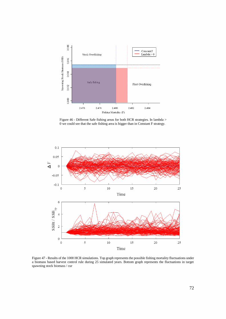
72

Figure 47 - Results of the 1000 HCR simulations. Top graph represents the possible fishing mortality fluctuations under a biomass based harvest control rule during 25 simulated years. Bottom graph represents the fluctuations in target spawning stock biomass / cur

Figure 46 - Different Safe fishing areas for both HCR strategies. In lambda >

0 we could see that the safe fishing area is bigger than in Constant F strategy.

73

4.- Discussion

Responses by individual species to climate change may disrupt their interactions

with others at the same or adjacent trophic levels (Walther et al., 2002). Recruitment in

fish populations has long been known to be a key process that is strongly influenced by

climate variability (Walther et al., 2002). Global warming is the main effect of climate

change. Although climate change generates widespread effects on marine and stock

dynamics, global warming does not necessarily lead to a monotonic decrease in the

expected biomass levels.

Increases in the surface temperature of the Iberian Atlantic fishery ground are

compatible with higher expected biomass and economic profit levels when the resource

is optimally exploited (Da Rocha & Gutierrez 2011). Also, small pelagic species are

subject to other environmental factors apart from temperature changes that affect natural

productivity. Summarizing, sardine biomass is affected by other environmental variables

that can mitigate the reduction in natural growth caused by climate change (Da Rocha &

Gutierrez 2011) being possible to manage in a sustainable and high profitable way.

Climate change may have a large impact on the distribution of maximum catch

potential (as a proxy of potential fisheries productivity) (Cheung et al. 2010) and has

direct implications in the calculus of management reference points. During the

investigation was demonstrated that a strong fishery stock dynamics knowledge could be

translated in better management measures and increase of economical profit for the

fisherman’s, avoiding the risk of collapse.

Stock dynamics are key to achieve a better management of the fishery. As we

demonstrated during the research, ignore the recruitment trend during the stock

assessment and management process generates an overestimation of the reference point

and ignores part of the risk of the harvest strategy. Therefore, summarizing, neglecting

the biological structure of the resource results in an underestimation of the optimal fishing

mortality (Tahvonen 2009).

Reference points are one of the main tools used by fishery managers to make

decision about the future catch options (Da Rocha 2012). For example, the European

Union, through the Common Fisheries Policy (CFP), wanted all the stock to be fished at

FMSY by 2015.

During the investigation, we demonstrated that Fmax is not an adequate

management reference point for fisheries. Fmax reference point could lead to

overexploitation of the stock and subsequently to an underperforming of the target

fishery. As basic information, we recommend a more precautionary reference point to

avoid an overexploitation situation of the resource and ensure the sustainability of the

fishery.

The proposition of elaborate a biomass based harvest control rule has direct

implications in policy design. All fisheries are managed to avoid the risk of the stock

collapsing, the aim should be to design policies that assign more weight to biomass goals

(like a biomass based HCR or constant escapement rules) (Da-Rocha & Mato-Amboage

2016). At the same time, constant fishing harvest control rule implementation amplifies

future risk by increasing the biomass volatility of the stock (Da-Rocha & Mato-Amboage

2016). Being the risk higher in constant F control policies, management politics as total

allowable catches and fixed quotas are not optimal (Da-Rocha & Mato-Amboage 2016).

74

In practical terms, it is hard to create a management strategy under the umbrella

of a biomass based harvest control rule. An easier way to implement these kinds of

measures in our fishery is a more precautionary harvest strategy taking as a reference a

more precautionary reference point. Other alternatives as reference point as 2/3Fmsy,

3/Fmsy or 90%Fmsy could be optimal for the future of the fishery.

75

5.- Conclusions

Modern fisheries management is moving towards a precautionary approach to

ensure the sustainability of the marine resurces (ICES, 1997). During this work, for

Sardina pilchardus in ICES VIIIc and IXa was demonstrated the risk of using Fmax as a

target reference point in the stock management and the necessity of being more

precautionary during the fishery management process.

Main outputs of the investigation were:

• Not include recruitment trend during the management of the fishery

ignores part of the risk of manage your fishery taking as a reference point

a constant F value.

• Biomass based harvest control rule decreases the probability of

biommass dropping under your Btrigger reference point. Constant fishing

mortality harvest control rule increases the risk of collapse of the fishery.

• Ignore the recruitment trend overestimates the yield per recruit value of

the fishery. Biomass based harvest control rule is more accurate to

estimate the future yield of the fishery.

77

References

A. Myers, R., & Mertz, G. (1998). Reducing uncertainty in the biological basis of fisheries

management by meta-analysis of data from many populations: a synthesis. Fisheries

Research, 37(1–3), 51–60.

About GFCM | General Fisheries Commission for the Mediterranean (GFCM) | Food and

Agriculture Organization of the United Nations. (2017).

Acom, I. C. M. (2014). ICES WGHANSA REPORT 2014 Report of the Working Group

on Southern Horse Mackerel, Anchovy and Sardine (WGHANSA) International Council

for the Exploration of the Sea, (June), 20–25.

Aldebert, (1988). Problemes d’exploitation du merlu dans le Golfe du Lion. FAO Rapp.

Peches, 395, 87–91.

Aldebert, Y., & Recasens, L. (1996). Comparison of methods for stock assessment of

European hake Merluccius in the Gulf of Lions (northwestern Mediterranean). Aquatic

Living resources/Ressources Vivantes Aquatiques. Nantes, 9(1), 13–22.

Assessment for All (a4a): enhancing fisheries modelling – EC-JRC (2015). Available at:

https://ec.europa.eu/jrc/en/scientific-tool/assessment-all-a4a-enhancing-fisheries-

modelling. (Accessed: 4th September 2017)

Beaugrand, G., & Reid, P. C. (2003). Long-term changes in phytoplankton, zooplankton

and salmon related to climate. Global Change Biology, 9(6), 801–817.

Beaugrand, G., Brander, K. M., Alistair Lindley, J., Souissi, S., & Reid, P. C. (2003).

Plankton effect on cod recruitment in the North Sea. Nature, 426(6967), 661–664.

Bouhlal, M., Ktari, N.H., (1975). Hake growth in gulf of Tunis, Tunisia area. Bulletin de

l’Institut National Scientifique et Technique d’Oceanographie et de Peche de Salambo.

Brunel, T., & Boucher, J. (2007). Long-term trends in fish recruitment in the north-east

Atlantic related to climate change. Fisheries Oceanography, 16(4), 336–349.

Chatterjee, S., & Hadi, A. S. (2006). Simple Linear Regression (pp. 21–51). John Wiley

& Sons, Inc.

Cheung, W. W. L., Lam, V. W. Y., Sarmiento, J. L., Kearney, K., Watson, R., & Pauly,

D. (2009). Projecting global marine biodiversity impacts under climate change scenarios.

Fish and Fisheries, 10(3), 235–251. (2009).

Cheung, W. W. L., Lam, V. W. Y., Sarmiento, J. L., Kearney, K., Watson, R., Zeller, D.,

& Pauly, D. (2010). Large-scale redistribution of maximum fisheries catch potential in

the global ocean under climate change. Global Change Biology, 16(1), 24–35.

78

Climate Change 2007 The Physical Science Basis. (2007). Retrieved from

https://www.ipcc.ch/pdf/assessment-report/ar4/wg1/ar4-wg1-frontmatter.pdf

Colloca, F., Cardinale, M., Maynou, F., Giannoulaki, M., Scarcella, G., Jenko, K., …

Fiorentino, F. (2013). Rebuilding Mediterranean fisheries: a new paradigm for ecological

sustainability. Fish and Fisheries, 14(1), 89–109.

Da Rocha, J.-M., & Gutierrez, M.-J. (2011). Lessons from the long-term management

plan for northern hake: could the economic assessment have accepted it? ICES Journal

of Marine Science, 68(9), 1937–1941.

Da Rocha, J.-M., Gutiérrez, M.-J., & Antelo, L. T. (2013). Selectivity, Pulse Fishing and

Endogenous Lifespan in Beverton-Holt Models. Environmental and Resource

Economics, 54(1), 139–154.

Da Rocha, J.-M., Gutierrez, M.-J., & Cervino, S. (2012). Reference points based on

dynamic optimization: a versatile algorithm for mixed-fishery management with

bioeconomic age-structured models. ICES Journal of Marine Science, 69(4), 660–669.

Da Rocha, J.-M., Gutiérrez, M.-J., & Villasante, S. (2014). Economic effects of global

warming under stock growth uncertainty: the European sardine fishery. Regional

Environmental Change, 14(1), 195–205.

Darby, C., & Flatman, S. (1994). Virtual population analysis: version 3.1 (Windows/Dos)

user guide.

Da-Rocha, J.-M., & Mato-Amboage, R. (2016). On the Benefits of Including Age-

Structure in Harvest Control Rules. Environmental and Resource Economics, 64(4), 619–

641.

Daskalov G. (1998). Using abundance indices and fishing effort data to tune catch-at-age

analyses of sprat Sprattus sprattus L., whiting Merlangius merlangus L. and spiny dogfish

Squalus acanthias L. in the Black Sea Using abundance indices and fishing effort data to

tune catch-at-age analyses of sprat Sprattus spratfus L., whiting Meulangius merlangus

and spiny dogfish Squalus acanthías L. in the Black Sea. Zaragoza : CIHEAM, 35, 215–

228.

Deroba, J. J., Butterworth, D. S., Methot, R. D., De Oliveira, J. A. A., Fernandez, C.,

Nielsen, A., … Hulson, P.-J. F. (2015). Simulation testing the robustness of stock

assessment models to error: some results from the ICES strategic initiative on stock

assessment methods. ICES Journal of Marine Science, 72(1), 19–30.

Dickey, D. A., & Fuller, W. A. (1979). Distribution of the Estimators for Autoregressive

Time Series with a Unit Root. Journal of the American Statistical Association, 74(366),

427.

FAO - EAFnet - EAF Planning and Implementation Tools - Harvest Strategies and

Control Rules. (n.d.). Retrieved September 4, 2017, from http://www.fao.org/fishery/eaf-

net/eaftool/eaf_tool_49/en

79

FAO. (n.d.). VPA Model. Retrieved September 4, 2017, from

ftp://ftp.fao.org/docrep/fao/003/x9026e/x9026e01.pdf (Accessed: 4th September 2017)

FAO. Reference points for fisheries management. Available at:

http://www.fao.org/docrep/003/v8400e/V8400E02.htm#ch2.2. (Accessed: 4th

September 2017)

Ferraton, F., Harmelin-Vivien, M., Mellon-Duval, C., & Souplet, A. (2007). Spatio-

temporal variation in diet may affect condition and abundance of juvenile European hake

in the Gulf of Lions (NW Mediterranean). Marine Ecology Progress Series 337, 197–208

Fiorentini, L., Dremière, P.-Y., Leonori, I., Sala, A., & Palumbo, V. (1999). Efficiency

of the bottom trawl used for the Mediterranean international trawl survey (MEDITS).

Fiorentino, F., Garofalo, G., De Santi, A., Bono, G., Giusto, G. B., & Norrito, G. (2003).

Spatio-temporal distribution of recruits (0 group) of Merluccius merluccius and Phycis

blennoides (Pisces, Gadiformes) in the Strait of Sicily (Central Mediterranean).

Hydrobiologia, 503, 223–236.

Fiorentino, F., Garofalo, G., Gristina, M., Gancitano, S., & Norrito, G. (2004). Some

relevant information on the spatial distribution of demersal resources, benthic

biocoenoses and fishing pressure in the Strait of Sicily. MedSudMed Technical

Documents, (2).

Francis, R. I. C. C., & Hilborn, R. (2011). Data weighting in statistical fisheries stock

assessment models. Canadian Journal of Fisheries and Aquatic Sciences, 68(6), 1124–

1138. http://doi.org/10.1139/f2011-025

General Fisheries Commission for the Mediterranean (2016). The State of Mediterranean

and Black Sea Fisheries. FAO.

GFCM, Fablet, R., Mellon, C., & de Pontual, H. (2007). Are hake otolith macrostructures

randomly deposited? Insights from an unsupervised statistical and quantitative approach

applied to Mediterranean hake otoliths. ICES Journal of Marine Science, 60(6), 31–57.

GFCM. (2016). Data Collection Reference Framework.

Gislason, H., Daan, N., Rice, J. C., & Pope, J. G. (2010). Size, growth, temperature and

the natural mortality of marine fish. Fish and Fisheries, 11(2), 149–158.

Group, M. W. (2012). International bottom trawl survey in the Mediterranean Instruction

Manual Version 6. MEDITS-Handbook, (April), 92.

Hannesson, R. (1975). Fishery Dynamics: A North Atlantic Cod Fishery. The Canadian

Journal of Economics, 8(2), 151.

Harley, C. D. G., Randall Hughes, A., Hultgren, K. M., Miner, B. G., Sorte, C. J. B.,

Thornber, C. S., … Williams, S. L. (2006). The impacts of climate change in coastal

marine systems. Ecology Letters, 9(2), 228–241.

80

Hodrick Edward C Prescott, R. J., Avery, R., Chari, V., Peter Hansen, L., Nelson, C. R.,

& Sargent, T. J. (n.d.). Postwar U.S. Business Cycles: An Empirical Investigation.

ICES WGHANSA REPORT 2014 International Council for the Exploration of the Sea

Conseil International pour l’Exploration de la Mer. (2014). Retrieved from

ICES. Acronyms ICES. (2012). ICES Advice, (1).

IPCC - Intergovernmental Panel on Climate Change. (n.d.). Retrieved September 4, 2017,

from

https://www.ipcc.ch/publications_and_data/publications_ipcc_fourth_assessment_repor

t_wg1_report_the_physical_science_basis.htm

Jardim, E., Millar, C., Scott, F., Osio, C. & Mosqueira, I. (2017). Assessment for All

initiative(a4a) The a4a Stock Assessment Modelling Framework.

Kell, L.T., Mosqueira, I., Grosjean, P., Fromentin, J-M., Garcia, D., Hillary, R., Jardim,

E., Mardle, S., Pastoors, M.A., Poos, J.J., Scott, F., Scott R.D. (2007). FLR: an open-

soiurce framework for the evaluation and development of management strategies. ICES

J. of Mar. Sci., 64: 640-646.

Kvamsdal, S. F., Eide, A., Ekerhovd, N.-A., Enberg, K., Gudmundsdottir, A., Hoel, A.

H., Vestergaard, N. (2016). Harvest control rules in modern fisheries management.

Elementa: Science of the Anthropocene, 4(0), 114.

Laurence Kell (2017). FLXSA: eXtended Survivor Analysis for FLR. R package version

2.5.20140808.

Lehodey, P., Alheit, J., Barange, M., Baumgartner, T., Beaugrand, G., Drinkwater, K.,

Werner, A. F. (2006). Climate Variability, Fish, and Fisheries. Retrieved from

Lejeusne, C., Chevaldonné, P., Pergent-Martini, C., Boudouresque, C. F., & Pérez, T.

(2010). Climate change effects on a miniature ocean: the highly diverse, highly impacted

Mediterranean Sea. Trends in Ecology & Evolution, 25(4), 250–260.

Levi, D., Patti, B., Rizzo, P., Lo Brutto, S., Parrinello, N., & Arculeo, M. (2004). Genetic

and morphometric variations of Mediterranean hake, Merluccius merluccius, in the Strait

of Sicily (central Mediterranean): implications for stock assessment of shared resources.

Ital. J. Zool, 71, 165–170.

Lo Brutto, S., Arculeo, M., Mauro, A., Scalisi, M., Cammarata, M., Parrinello, N.,

Cammarata Nicolò Parrinello, M. (1998). Allozymic variation in Mediterranean hake

Merluccius merluccius (Gadidae) Italian Journal of Zoology J. Zool, 65(65), 1–49.

Ludwig, D., & Walters, C. J. (1981). Measurement Errors and Uncertainty in Parameter

Estimates for Stock and Recruitment. Canadian Journal of Fisheries and Aquatic

Sciences, 38(96072), 711–720.

81

Magnusson, K. (1995). An overview of the multispecies VPA, theory and applications.

Reviews in Fish Biology and Fisheries, 5(2), 195–212.

María, J., & Cutrín, G. (2016). Reconciling yield stability with international fisheries

agencies precautionary preferences: The role of non-constant discount factors in age

structured models.

Mid-term strategy (2017–2020) towards the sustainability of Mediterranean and Black

Sea fisheries (Mid-term strategy). (2016).

Morales-Nin, B., & Aldebert, Y. (1997). Growth of juvenile Merluccius merluccius in the

Gulf of Lions (NW Mediterranean) based on otolith microstructure and length-frequency

analysis. Fisheries Research, 30(1–2), 77–85.

Morales-Nin, B., Tores, G. J., Lombarte, A., & Recasens, L. (1998). Otolith growth and

age estimation in the European hake. Journal of Fish Biology, 53(6), 1155–1168.

PennState, E. C. of S. (n.d.). 1.1 - What is Simple Linear Regression? | STAT 501.

Retrieved September 4, 2017.

Pepin, P. (1991). Effect of Temperature and Size on Development, Mortality, and

Survival Rates of the Pelagic Early Life History Stages of Marine Fish. Canadian Journal

of Fisheries and Aquatic Sciences, 48(3), 503–518.

Punt, A. E., Butterworth, D. S., de Moor, C. L., De Oliveira, J. A. A., & Haddon, M.

(2016). Management strategy evaluation: best practices. Fish and Fisheries, 17(2), 303–

334.

Ralston, S., Punt, A. E., Hamel, O. S., DeVore, J. D., & Conser, R. J. (2011). A meta-

analytic approach to quantifying scientific uncertainty in stock assessments. Fishery

Bulletin, 109(2), 217–232.

Reid, P. C., Borges, M. de F., & Svendsen, E. (2001). A regime shift in the North Sea

circa 1988 linked to changes in the North Sea horse mackerel fishery. Fisheries Research,

50(1–2), 163–171.

GFCM. Scientific Advisory Committee on Fisheries (SAC) Report of the Workshop on

the assessment of management measures (WKMSE). (2017).

GFCM. Scientific Advisory Committee on Fisheries (SAC) Working Group on Stock

Assessment of Demersal Species (WGSAD). (GFCM, 2016).

Shepherd, J. (1999). Extended survivor’s analysis: An improved method for the analysis

of catch-at-age data and abundance indices. ICES Journal of Marine Science, 56(5), 584–

591.

Smith, A., Sainsbury, K. J. & Stevens, R. A. (1999). Implementing effective fisheries-

management systems – management strategy evaluation and the Australian partnership

approach. ICES J. Mar. Sci. 56, 967–979

82

ICES. Study Group on The Precautionary Approach to Fisheries Management

International Council for the Exploration of the Sea Conseil International pour

l’Exploration de la Mer. (1998).

Sumaila, U. R., Cheung, W. W. L., Lam, V. W. Y., Pauly, D., & Herrick, S. (2011).

Climate change impacts on the biophysics and economics of world fisheries. Nature

Climate Change, 1(9), 449–456.

Tahvonen, O. (2008). Harvesting an Age-Structured Population as Biomass: Does It

Work? Natural Resource Modeling, 21(4), 525–550.

Tahvonen, O. (2009). Economics of harvesting age-structured fish populations. Journal

of Environmental Economics and Management, 58(3), 281–299.

Tahvonen, O. (2009). Optimal Harvesting of Age-structured Fish Populations. Marine

Resource Economics.

Tasker, M. L. (Ed. (2008). The effect of climate change on the distribution and abundance

of marine species in the OSPAR Maritime Area. ICES Cooperative Research Report No.

293.

Uriarte, A., Prouzet, P., & Villamor, B. (1996). Bay of Biscay and Ibero Atlantic anchovy

populations and their fisheries. Scientia Marina, 60(2), 237–255.

Walther, G. R., Post, E., Convey, P., Menzel, A., Parmesan, C., Beebee, T. J. C., …

Bairlein, F. (2002). Ecological responses to recent climate change. Nature, 416(6879),

389–395.

Worm, B., Hilborn, R., Baum, J. K., Branch, T. A., Collie, J. S., Costello, C., … Zeller,

D. (2009). Rebuilding Global Fisheries. Science, 325(5940), 578–585.

85

Annex – Codes Chapter 1

1.- Extended Survivor Analysis

library(FLCore)

library(FLEDA)

library(FLXSA)

library(FLAssess)

library(FLash)

require(ggplotFL)

require(plyr)

require(FLBRP)

#read stock file

aa.stk <- readFLStock("HKE1216.IND", no.discards=TRUE)

catch(aa.stk)

landings(aa.stk)

catch(aa.stk)/landings(aa.stk)

# catch.n(aa.stk)

# landings.n(aa.stk)

# catch.wt(aa.stk)

# landings.wt(aa.stk)

# quantSums(catch.n(aa.stk)*catch.wt(aa.stk))

bubbles(age~year, data=(catch.n(aa.stk)), bub.scale=5)

bubbles(age~year, data=(catch.wt(aa.stk)), bub.scale=5)

mat(aa.stk)

m(aa.stk)

##### SOP correction

sop(aa.stk,"landings")

86

landings(aa.stk)*sop(aa.stk,"landings")

landings(aa.stk)<-catch(aa.stk)

landings(aa.stk)/catch(aa.stk)

#set up the stock

units(harvest(aa.stk))<-"f"

range(aa.stk)["minfbar"] <- 1

range(aa.stk)["maxfbar"] <- 5

#Set the plus group

aa.stk <- setPlusGroup(aa.stk, 6)

# #Remove 2003

# aa.stk<-window(aa.stk, start=2004, end=2013)

#read index (tuning file)

aa.idx <- readFLIndices("TUNEFF.dat")

#Remove age until 4

# aa.idx<-window(aa.idx, start=2005, end=2013)

aa.idx[[1]]<- trim(aa.idx[[1]], age=0:2)

bubbles(age~year, data=(index(aa.idx[[1]])), bub.scale=6)

#plot the stock

plot(aa.stk)

#####################################

######################################

#### sensitivity analisys changing rage different setting changing rage

#######################################

87

#FSE 0.5

FLXSA.control.aa <- FLXSA.control(x=NULL, tol=1e-09, maxit=30,

min.nse=0.3, fse=0.5,

rage=0, qage=1, shk.n=TRUE, shk.f=TRUE, shk.yrs=3,

shk.ages=3,

window=100, tsrange=20, tspower=3, vpa=FALSE)




shk.ages=3,





shk.ages=3,





shk.ages=3,


#FSE 1


min.nse=0.3, fse=1,


shk.ages=3,





shk.ages=3,


88


min.nse=0.3, fse=1,


shk.ages=3,



min.nse=0.3, fse=1,


shk.ages=3,


#FSE 2


min.nse=0.3, fse=2,


shk.ages=3,





shk.ages=3,



min.nse=0.3, fse=2,


shk.ages=3,



min.nse=0.3, fse=2,


shk.ages=3,

89


#Running the assessments with different settings changing q at age

aa.xsa <- FLXSA(aa.stk, aa.idx, FLXSA.control.aa)

aa.xsa1 <- FLXSA(aa.stk, aa.idx, FLXSA.control.aa1)











#Add the results to the stock files

aa.stk <- aa.stk+aa.xsa

aa.stk1 <- aa.stk+aa.xsa1










aa.stk11<- aa.stk+aa.xsa11

90

stocks <-

FLStocks(aa.stk,aa.stk1,aa.stk2,aa.stk3,aa.stk4,aa.stk5,aa.stk6,aa.stk7,aa.stk8,aa.stk9,aa.

stk10,aa.stk11)

names(stocks)<-

c("0.5r0q1","0.5r0q2","0.5r0q3","0.5r0q4","1r0q1","1r0q2","1r0q3","1r0q4",

"2r0q1","2r0q2","2r0q3","2r0q4")

plot(stocks)

plot(aa.stk+aa.xsa4)

91

2.- Deterministic a4a

# MI PROYECTO:

#1.- Paquetes:

library(FLa4a)

library(XML)

library(reshape2)

library(diagram)

library(plot3D)

library(FLCore)

library(FLXSA)

library(ggplotFL)

library(ggplot2)

#

rm(list=ls())

cat("\014")

#

# Working Directory

setwd("~/MSE Project/MSE/2017/StraitOfSicily/HKE/a4a/Length

structured/Deterministic a4a")

getwd()

# Leemos todos los archivos:

# read stock file

HKE.stk <- readFLStock("HKE1216.IND", no.discards=T)

# Set up the stock (create the empty matrix)

92

units(harvest(HKE.stk))<-"f"

range(HKE.stk)["minfbar"] <- 2

range(HKE.stk)["maxfbar"] <- 4

# Set the plus group

HKE.stk <- setPlusGroup(HKE.stk, 7)

# read index (tuning file)

HKE.idx <- readFLIndices("TUNEFF.DAT")

HKE.idx <- FLIndices(trim(HKE.idx[[1]],age=1:7))

bubbles(age~year, data=(index(HKE.idx[[1]])), bub.scale=10)

plot(HKE.stk)

catch.n(HKE.stk)[catch.n(HKE.stk)==0] <- 0.01

for (i in 1:length(HKE.idx)){

index(HKE.idx[[i]])[index(HKE.idx[[i]])==0] <- 0.01

}

# 5.- CORRIENDO EVALUACIONES

# En el modelo de evaluacion a4a, la estructura del modelo esta definida por

submodelos,

# los cuales son varias artes de un modelo de captura por edad que requiere varias

asumpciones.

# Estos son los 5 submodelos:

# Modelo para F-at-age

# Modelo para la estructura de edad inicial

# Modelo para el reclutamiento

# Una lista de modelos para la observacion de la varianza de la captura por edad

e indices de abundancia

93

# Llevado a la practica: Fijamos los modelos de varianza y los modelos de

estructura de edad iniciales,

# pero esto en teoria puede cambiar

# Los submodelos usan modelos lineales.

# Existen 2 tipos de evaluaciones disponibles en a4a:

# Ajuste del proceso de gestion: No estima ni computa covarianzas y es mas rapido

de ejecutar

# Ajuste completo de la evaluacion: Nos devuelve parametros y sus covarianzas

y tarda mas tiempo en ajustar

# 5.1.- Stock assessment model details

# El modelo estadistico de captura por edad esta basado en la ecuacion de Baranov

de captura y en el indice de capturabilidad.

# Todos los detalles de las ecuaciones estan en el manual (pag.37)

# 5.2.- Rapido y sucio

# He aqui un ejemplo de uso del modelo de evaluacion. Se ve como los ajustes

default del modelo de ev. funcionan bien.

# fit <- sca(HKE.stk, HKE.idx)

# Para inspeccionar el resumen de la evaluacion del stock, el cual esta construido

con tendencias de:

# mortalidad pesquera,

# desove,

# ssb,

# captura y

# reclutas

# El usuario debe anadir el objeto a4afit al archivo original FLStock usando el +

method

94

fit <- sca(HKE.stk, FLIndices(HKE.idx))

fmod2 <- ~ s(age, k=3) + s(year, k = 3)

qmodel <- list(~ factor(age))

srmodB <- ~ bevholt(CV=0.1)

fit <- sca(HKE.stk, FLIndices(HKE.idx),

fmodel=fmod2,qmodel=qmodel,srmodel=srmodB)

stk <- HKE.stk + fit

plot(stk)

persp3D(z=harvest(fit)[drop=TRUE],

x=as.numeric(dimnames(harvest(fit))[[1]]), y=as.numeric(dimnames(harvest(fit))[[2]]),

facets = FALSE, curtain = TRUE)

ribbon3D( z = stock.n(fit)[drop=TRUE], x=

as.numeric(dimnames(stock.n(fit))[[1]]), y= as.numeric(dimnames(stock.n(fit))[[2]]),

facets = FALSE, curtain = TRUE)

# 5.3- Diagnosticos

# Un conjunto de graficos que sriven para comprobar la calidad de las

asumpciones se encuentra implementado.

# Lo mas normal es mirar los log-residuales estandarizados para ver los resultados

parciales de grandes varianzas.

# Hay que recordad que la estandarizacion tiene que dar residuales con varianza

1.

# Estos resultados permiten al usuario identificar desviaciones de la asumpcion

lognormal.

res <- residuals(fit,HKE.stk,HKE.idx)

bubbles(res)

95

qqmath(res)

plot(fit,HKE.stk)

plot(fit, HKE.idx)

# Para obtener la informacion sobre la probabilidad hay que ajustar el metodo

fitSumm()

# Este metodo nos va a ayudar a extraer la informacion sobre la probabilidad,

numero de parametros...

# Los metodos AIC() y BIC() nos ayudaran a computar la informacion criterio.

fitSumm(fit)

AIC(fit)

BIC(fit)

97

3.- Stochastic a4a Analysis

#########################################################

### ###

### "THE SCRIPT" - MAY 2017 ###

### Eduardo Sánchez Llamas - Master Thesis ###

### ###

### a4a ###

#########################################################

# SCRIPT INDEX (GENERAL)

# install.packages(c("copula","triangle"))

# install.packages(c("FLCore", "FLa4a"), repos="http://flr-project.org/R")

library(FLa4a)

library(XML)

library(reshape2)

library(plot3D)

library(FLCore)

library(FLXSA)

library(ggplotFL)

#

rm(list=ls())

cat("\014")

#

setwd("~/MSE Project/MSE/2017/StraitOfSicily/HKE/a4a/Stochastic a4a/Data")

#setwd("~/HAKE 12-16/MSE-StrategyXSA/Length structured")

98

################################################################

#################

## ##

## Functions ##

## ##

################################################################

#################

# recode Gadget's length categories

qt2qt <- function(object, id=5, split="-"){

qt <- object[,id]

levels(qt) <- unlist(lapply(strsplit(levels(qt), split=split), "[[", 2))

as.numeric(as.character(qt))

}

# function to check import and do some massage

cim <- function(object, n, wt, hrv="missing"){

v <- object[sample(1:nrow(object), 1),]

c1 <-

c(n[as.character(v$V5),as.character(v$V1),1,as.character(v$V2)]==v$V6)

c2 <-

c(wt[as.character(v$V5),as.character(v$V1),1,as.character(v$V2)]==v$V7)

if(missing(hrv)){

c1 + c2 == 2

} else {

c3 <-

c(hrv[as.character(v$V5),as.character(v$V1),1,as.character(v$V2)]==v$V8)

c1 + c2 + c3 == 3

}

}

# plot for S4 data structures with diagram

plotS4 <- function(object, linktext="typeof", main="S4 class", ...){

6

args <- list(...)

obj <- getClass(as.character(object))

99

df0 <- data.frame(names(obj@slots), unlist(lapply(obj@slots, "[[", 1)))

nms <- c(t(df0))

nslts <- length(nms)/2

M <- matrix(nrow = length(nms), ncol = length(nms), byrow = TRUE, data = 0)

for(i in 1:nslts){

M[i*2,i*2-1] <- linktext

}

args$A=M

args$pos=rep(2, length(nms)/2)

args$name = nms

args$main=main

do.call("plotmat", args)

}

################################################################

#################

## ##

## Introducing Data ##

## ##

################################################################

#################

# Catch

cth.orig <- read.table("cth_mean_weight_kg_review.txt",

header=FALSE,skip=5,fill = TRUE)

head(cth.orig)

cth.orig[,5] <- qt2qt(cth.orig)

cth.n <- acast(V5~V1~1~V2~1~1, value.var="V6", data=cth.orig)

cth.wt <- acast(V5~V1~1~V2~1~1, value.var="V7", data=cth.orig)

dnms <- dimnames(cth.n)

names(dnms) <- names(dimnames(FLQuant()))

100

names(dnms)[1] <- "len"

cth.n <- FLQuant(cth.n, dimnames=dnms)

cth.wt <- FLQuant(cth.wt, dimnames=dnms)

HKE.stk <- FLStockLen(catch.n=cth.n,

catch.wt=cth.wt)

cim(cth.orig,cth.n,cth.wt)

HKE.stk <- FLStockLen(catch.n=cth.n,catch.wt=cth.wt)

# Survey

idx.orig <- read.table("idx_mean_weight_kg.txt", skip=5, header=FALSE, fill =

TRUE)

idx.orig[,5] <- qt2qt(idx.orig)

idx.n <- acast(V5~V1~1~V2~1~1, value.var="V6", data=idx.orig)

idx.wt <- acast(V5~V1~1~V2~1~1, value.var="V7", data=idx.orig)

dnms <- dimnames(idx.n)



idx.n <- FLQuant(idx.n, dimnames=dnms)

idx.wt <- FLQuant(idx.wt, dimnames=dnms)

HKE.idx <- FLIndex(index=idx.n, catch.n=idx.n, catch.wt=idx.wt)

effort(HKE.idx)[] <- 100

m(HKE.stk)[]<-0.05

mat(HKE.stk)[]<-m.spwn(HKE.stk)[]<-harvest.spwn(HKE.stk)[]<-0

## careful, landings are not retained in the stock object after length to age

conversion

101

landings(HKE.stk)[]<-

c(3792.2,3395.5,3284.4,3444.7,2532.8,3306.1,3467.4,4415.0,4081.8)

################################################################

#################

## ##

## Adding uncertainty to growth parameters ##

## ##

################################################################

#################

#Von Bert. Model

vbObj <- a4aGr(

grMod=~linf*(1-exp(-k*(t-t0))),

grInvMod=~t0-1/k*log(1-len/linf),

params=FLPar(linf=100, k=0.116, t0=-0.6, units=c("cm","ano-1","ano"))

)

lc=100

predict(vbObj, len=lc)

predict(vbObj, t=predict(vbObj, len=lc))

predict(vbObj, len=5:20+0.5)

predict(vbObj, t=1:20+0.5)

prediction <- predict(vbObj, len=seq(8, 74, length = 200))

predictiontime <- predict(vbObj, t=seq(0.1,10, length=200))

plot(seq(8, 74, length = 200), prediction, xlab="length (cm)", ylab="Age (years)")

102

plot(seq(0.1,10, length=200), predictiontime, ylab="length (cm)", xlab="Age

(years)")

##############################################

## ##

## Ages without uncertainty: ##

## cth.n <- l2a(catch.n(HKE.stk), vbObj) ##

## ##

##############################################

# 3.2.- AÑADIENDO INCERTIDUMBRE CON LA DISTRIBUCIÓN

NORMAL MULTIVARIANTE

# Adding uncertainty with a normal multivariate distribution

cm <- diag(c(1,1,1))

cm[1,2] <- cm[2,1] <- -0.5

cv <- 0.2

p <- c(linf=100, k=0.116, t0=-0.6)

vc <- matrix(1, ncol=3, nrow=3)

l <- vc

l[1,] <- l[,1] <- p[1]*cv

k <- vc

k[,2] <- k[2,] <- p[2]*cv

t <- vc

t[3,] <- t[,3] <- p[3]*cv

mm <- t*k*l

diag(mm) <- diag(mm)^2

mm <- mm*cm

all.equal(cm, cov2cor(mm)) # Correlation = "True"

103

vbObj <- a4aGr(grMod=~linf*(1-exp(-k*(t-t0))),


params=FLPar(linf=p["linf"], k=p["k"], t0=p["t0"], units=c("cm","ano-

1","ano")), vcov=mm)

# Data is following a normal multivariate distribution

vbObj@params

dim(vbObj@params)

# Simulating 1000 iterations:

vbNorm <- mvrnorm(10000,vbObj)

vbNorm@params

dim(vbNorm@params)

ages <- predict(vbNorm, len=5:10+0.5)

dim(ages)

ages[,1:10]

par(mfrow=c(1,1))

hist(c(params(vbNorm)["linf",]), main="linf", xlab="")

hist(c(params(vbNorm)["k",]), main="k", prob=TRUE, xlab="")

hist(c(params(vbNorm)["t0",]), main="t0", xlab="")

splom(data.frame(t(params(vbNorm)@.Data)),

pch=".",par.settings=list(plot.symbol=list(pch=50, cex=1.5, col=1)))

104

boxplot(t(predict(vbNorm, t=0:25+0.5)),xlab="Years",ylab="Length")

################################################################

#################

## ##

## Natural Mortality matrix uncertainty ##

## ##

################################################################

#################

shape4 <- FLModelSim(model=~exp(-age-0.5))

level4 <- FLModelSim(model=~k^0.66*t^0.57,

params=FLPar(k=0.116, t=10),

vcov=array(c(0.002, 0.01,0.01, 1), dim=c(2,2)))

trend4 <- FLModelSim(model=~1+b, params=FLPar(b=0.5), vcov=matrix(0.02))

m4 <- a4aM(shape=shape4, level=level4, trend=trend4)

m4 <- mvrnorm(250,m4)

m4

m4@level

params(trend(m4))

m4 <- a4aM(shape=shape4,

level=mvrnorm(100,level4),trend=mvrnorm(100,trend4))

params(shape(m4))

#

linf <- 100

k <- 0.116

mm <- matrix(NA, ncol=2, nrow=2)

diag(mm) <- c((linf*0.1)^2,(k*0.1)^2)

mm[upper.tri(mm)] <- mm[lower.tri(mm)] <- c(0.05)

105

cov2cor(mm)

mgis2 <-

FLModelSim(model=~k*(linf/len)^1.5,params=FLPar(linf=linf,k=k),vcov=mm)

pars <- list(list(a=90,b=110), list(a=0.05,b=0.15,c=0.110))

mgis2 <- mvrtriangle(10000, mgis2, paramMargins=pars)

mgis2

par(mfrow=c(1,1))

hist(c(params(mgis2)["linf",]), main="linf", xlab="")

hist(c(params(mgis2)["k",]), main="k", prob=TRUE, xlab="")

splom(data.frame(t(params(mgis2)@.Data)),


m5<-m4

shape(m5) <- mgis2

m(m5, nao=1)

dim(m(m5, nao=1))

m(m4)

rngquant(m4)<-c(0,6)

dim(m(m4))

m(m4)

rngyear(m4)<-c(2007,2015)

m(m4)

dim(m(m4))

flq <- m(m4)

106

bwplot(data~factor(age)|year,

data=flq,

par.settings=list(plot.symbol=list(cex=0.2, col="gray50"),

box.umbrella=list(col="gray40"),

box.rectangle=list(col="gray30")),

ylab="M", xlab="age (years)", scales=list(x=list(rot=90)))

################################################################

#################

## ##

## Reading the XSA object ##

## (to get assumptions on natural mortality and maturity at age) ##

## ##

################################################################

#################

## XSA object is ages 1 to 7

aaXSA.stk <- readFLStock("~/MSE

Project/MSE/2017/StraitOfSicily/HKE/a4a/Stochastic a4a/Data/HKE1216.IND",

no.discards=TRUE) #only commercial data

aaXSA.stk <- trim(aaXSA.stk, age=0:6)

aaXSA.idx <- readFLIndices("~/MSE

Project/MSE/2017/StraitOfSicily/HKE/a4a/Stochastic a4a/Data/TUNEFF.DAT")

name(aaXSA.idx[[1]]) <- "MEDITS_12-16"

# Length to age

aStk <- l2a(HKE.stk, vbNorm, plusgroup=6) #

aIdx <- l2a(HKE.idx, vbNorm) #

# Intro M into the object:

107

#mortalidad <- trim(m(m4), age=0:6)

#aStk@m <- mortalidad

#aStk@m <- mortalidad

####

# aStk@m <- m(m4)

#aStk <- trim(aStk, age=1:6)

units(aStk)[1:17] <- as.list(c(rep(c("tonnes","thousands","kg"),4),

rep("NA",2),"f",rep("NA",2)))

[email protected][] <- 0; [email protected][] <- 0; aStk@discards <-

computeDiscards(aStk)

landings(aStk)[]<-

c(3792.2,3395.5,3284.4,3444.7,2532.8,3306.1,3467.4,4415.0,4081.8)

catch(aStk)[]<-computeCatch(aStk)

## we need to check SOP correction

(catch(aStk)-landings(aStk))/landings(aStk)*100

## PROBLEM! for now assuming landings = computed catches (catch.n *

catch.wt)

[email protected][[email protected]==0] <- 0.001

landings(aStk)<-catch(aStk)

landings.n(aStk) <- catch.n(aStk)

landings.wt(aStk) <-catch.wt(aStk)

108

stock.wt(aStk) <- catch.wt(aStk)

dim(aaXSA.stk@m)

dim(aStk@m)

#aStk@m<- aaXSA.stk@m

#aStk@mat <- aaXSA.stk@mat

#[email protected] <- [email protected]

## using same m, maturity ogive, m.spawn as in XSA assessment

my.iter = 100

for (i in 1:my.iter){

aStk@m[,,,,,i]<- aaXSA.stk@m

aStk@mat[,,,,,i] <- aaXSA.stk@mat

[email protected][,,,,,i] <- [email protected]


}

range(aStk)["minfbar"] <- 2

range(aStk)["maxfbar"] <- 4

aStk <- trim(aStk, age=1:6)

[email protected] <- aIdx@index

aIdx <- trim(aIdx, age=1:6)

aIdx@range["plusgroup"] <- 6

aIdx@index[aIdx@index==0] <- 0.001


109

range(aIdx)[c("startf", "endf")] <- c(2,4)

# aStk@range["min"] <- 1

summary(aIdx)

summary(aStk)

fmod <- ~factor(age) + factor(year)

qmod <- list(~s(age, k=4))

n1mod <- ~s(age,k=5)

# Tests

fit <- a4aSCA(aStk,FLIndices(aIdx),fmodel=~factor(age) + factor(year))

out <- aStk + fit

plot(out)

res <- FLQuants("Yield(t)" =landings(out),

"Fbar(1-3)" = fbar(out),

"R(age 1)" = R <- stock.n(out)[1,,,,],

"SSB(t)" = ssb(out))

res

ggsave("retro.png",last_plot())

###### Choose the final model and save it

plot(out)

110

ggsave("final.png",last_plot())

fbar(out)

quantSums(stock.n(out)*stock.wt(out))

ssb(out)

rec(out)

harvest(out)

#--------------------------------------------------------

# Y/R

#--------------------------------------------------------

library(FLBRP)

#BRP

yprec <- brp(FLBRP(out))

yprec

refpts(yprec)

refpts(yprec)<-refpts(yprec)[c(4)]#without F crash

plot(ypr(yprec)~fbar(yprec),type='l')

plot(yprec)

ggsave("YPR.png",last_plot())

save(HKE.stk,HKE.idx, out, fit, aStk,aIdx,file="a4aoutputs.RData")

load("a4aoutputs.RData")

4.- Short Term Forecasting

XSA

# short_term_forecast.R

# Copyright 2013 Finlay Scott and Chato Osio

111

# Maintainer: Finlay Scott, JRC, [email protected]

# This program is free software; you can redistribute it and/or modify

# it under the terms of the GNU General Public License as published by

# the Free Software Foundation; either version 2 of the License, or

# (at your option) any later version.

#

# This program is distributed in the hope that it will be useful,

# but WITHOUT ANY WARRANTY; without even the implied warranty of

# MERCHANTABILITY or FITNESS FOR A PARTICULAR PURPOSE. See the

# GNU General Public License for more details.

#

# You should have received a copy of the GNU General Public License

along

# with this program; if not, write to the Free Software Foundation,

Inc.,

# 51 Franklin Street, Fifth Floor, Boston, MA 02110-1301 USA.

#---------------------------------------------------------------------

-----

# Generic script for running short-term forecasts (STF).

# This script assumes that have already run your assessment and that you

have a fully specified age-structured FLStock object

#------------------------------------------------------------------

# Example data set - use your own

# You need a full specified FLStock object

# Here I'm loading a dummy stock object

# load("../data/stk.RData")

# Load your own data, probably using the load() function

# Quick check that the stock object is correct

summary(aa.stk4)

plot(aa.stk4)

# For the STF we would like to run a F0.1 scenario

# Use FLBRP to get F0.1

stk_brp <- brp(FLBRP(aa.stk4))

refpts(stk_brp)

f01 <- c(refpts(stk_brp)["f0.1","harvest"])

##### f01 estimated with NOAA

# Is this number sensible?

# We also need F status quo - the geometric mean of the last X years

# Here we use 3 years

no_stk_years <- dim(rec(aa.stk4))[2]

no_fbar_years <- 3 # Or set your own as appropriate

fbars <- fbar(aa.stk4)[,(no_stk_years - no_fbar_years + 1):no_stk_years]

fbar_status_quo <- exp(mean(log(c(fbars))))

# fbar_status_quo <- c(fbar(aa.stk4)[,ac(2013)])

#---------------------------------------------------------------------

-----

# STF

# Here we run the STF for 3 years, 2013, 2014, 2015

# You can change these as appropriate

# The first year of the STF should be the next one after the final year

in your stock data

112

# For example, the final year in the dummy stk object is 2012 so the

first year of the STF is 2013

stf_years <- c(2016,2017,2018)

no_stf_years <- length(stf_years)

# Set up the future stock object.

# Here we use the default assumptions about what happens to weights,

maturity and selection pattern in the future

# (e.g. weights are means of the last 3 years)

# NOTE: You may want to change some of these assumptions by hand

# See the help page for stf: ?stf for more details

stf_stk <- stf(aa.stk4, nyears = no_stf_years, wts.nyears = 3)

# Set up future recruitment to be mean of last X years

# Here we set as geometric mean of the last 3 years

no_rec_years <- 3 # Change number of years as appropriate

recs <- rec(aa.stk4)[,(no_stk_years - no_rec_years + 1):no_stk_years]

mean_rec <- exp(mean(log(c(recs))))

# We are going to run several F scenarios for the STF

# The scenarios are based on 'F status quo', which we calculated above

as the mean F of the last X years

# An STF is for three years - you could change this but if you do you

will have to hack the code below

# For a three year STF the F pattern is:

# year 1: fbar_status_quo

# year 2: fbar_status_quo * fbar_multiplier


# The fbar_multiplier is the same for years 2 and 3

# We are going to run several STFs with different values for the

fbar_multiplier

# The fbar_multiplier ranges from 0.1 to 2 by 0.1

fbar_multiplier <- seq(from = 0, to = 2, by = 0.1)

# We are going to build a data.frame that builds these scenarios

# Each column in the dataframe is a year

# Each row is a scenario

# Set up the fbar scenarios - note that if you project for more than 3

years you will need to add more columns / years to the matrix

fbar_scenarios <- cbind(rep(fbar_status_quo,length(fbar_multiplier)),

fbar_multiplier*fbar_status_quo,

fbar_multiplier*fbar_status_quo)

# Add the F0.1 scenario as a final scenario

fbar_scenarios <- rbind(fbar_scenarios, c(fbar_status_quo,f01,f01))

# There are various results we want to extract from the STF

# Make an empty matrix in which to store the results

stf_results <- matrix(NA,nrow = nrow(fbar_scenarios),ncol = 10)

# Change the column names to reflect years

colnames(stf_results) <-

c('Ffactor','Fbar','Catch_2015','Catch_2016','Catch_2017','Catch_2018'

,'SSB_2017','SSB_2018','Change_SSB_2017-2018(%)','Change_Catch_2015-

2016(%)')

# Store the FLStock each time

stk_stf <- FLStocks()

# Loop over the scenarios

for (scenario in 1:nrow(fbar_scenarios)) {

cat("Scenario: ", scenario, "\n")

113

# Make a target object withe F values for that scenario

ctrl_target <- data.frame(year = stf_years,

quantity = "f",

val = fbar_scenarios[scenario,])

# Set the control object - year, quantity and value for the moment

ctrl_f <- fwdControl(ctrl_target)

# Run the forward projection. We include an additional argument, maxF.

# By default the value of maxF is 2.0

# Here we increase it to 10.0 so that F is not limited

stk_stf_fwd <- fwd(stf_stk, ctrl = ctrl_f, sr = list(model="mean",

params=FLPar(a = mean_rec)), maxF = 10.0)

## Check it has worked - uncomment out to check scenario by scenario

#plot(stk_stf_fwd)

# Store the result - if you want to, comment out if unnecessary

stk_stf[[as.character(scenario)]] <- stk_stf_fwd

# Fill results table

stf_results[scenario,1] <- fbar_scenarios[scenario,2] /

fbar_scenarios[scenario,1] # fbar status quo ratio

stf_results[scenario,2] <- fbar(stk_stf_fwd)[,ac(2018)] # final stf

year

stf_results[scenario,3] <- catch(stk_stf_fwd)[,ac(2015)] # last 'true'

year

stf_results[scenario,4] <- catch(stk_stf_fwd)[,ac(2016)] # 1st stf

year

stf_results[scenario,5] <- catch(stk_stf_fwd)[,ac(2017)] # 2nd stf

year

stf_results[scenario,6] <- catch(stk_stf_fwd)[,ac(2018)] # final stf

year

stf_results[scenario,7] <- ssb(stk_stf_fwd)[,ac(2017)] # 2nd stf year

stf_results[scenario,8] <- ssb(stk_stf_fwd)[,ac(2018)] # final stf

year

# Change in SSB

stf_results[scenario,9] <- (ssb(stk_stf_fwd)[,ac(2018)]-

ssb(stk_stf_fwd)[,ac(2017)])/ssb(stk_stf_fwd)[,ac(2017)]*100 # change

in ssb in last two stf years

stf_results[scenario,10] <- (catch(stk_stf_fwd)[,ac(2017)]-

catch(stk_stf_fwd)[,ac(2015)])/catch(stk_stf_fwd)[,ac(2015)]*100 #

change in catch from true year, to 2nd to last stf year

}

# Look at the table of results

View(stf_results)

# export this if necessary

write.csv(stf_results, file="stf_results_fr.csv")

# Plotting

# Plotting is not necessary for the report but here is a crude one anyway

plot(window(stk_stf, start=2008, end=2018))

ggsave("stf.png",last_plot())

114

Deterministic a4a

#-------------------------------------------------

# a4a Short Term Forecast

#-------------------------------------------------

# short_term_forecast.R

# Copyright 2013 Finlay Scott and Chato Osio

# Maintainer: Finlay Scott, JRC, [email protected]

# This program is free software; you can redistribute it and/or modify

# it under the terms of the GNU General Public License as published by

# the Free Software Foundation; either version 2 of the License, or

# (at your option) any later version.

#

# This program is distributed in the hope that it will be useful,

# but WITHOUT ANY WARRANTY; without even the implied warranty of

# MERCHANTABILITY or FITNESS FOR A PARTICULAR PURPOSE. See

the

# GNU General Public License for more details.

#

# You should have received a copy of the GNU General Public License along

# with this program; if not, write to the Free Software Foundation, Inc.,

# 51 Franklin Street, Fifth Floor, Boston, MA 02110-1301 USA.

#--------------------------------------------------------------------------

# Generic script for running short-term forecasts (STF).

# This script assumes that have already run your assessment and that you have a

fully specified age-structured FLStock object

#------------------------------------------------------------------

aa.stk4 <- stk1

115

# Example data set - use your own

# You need a full specified FLStock object

# Here I'm loading a dummy stock object

# load("../data/stk.RData")

# Load your own data, probably using the load() function

# Quick check that the stock object is correct

summary(aa.stk4)

plot(aa.stk4)

# For the STF we would like to run a F0.1 scenario

# Use FLBRP to get F0.1

stk_brp <- brp(FLBRP(aa.stk4))

refpts(stk_brp)

f01 <- c(refpts(stk_brp)["f0.1","harvest"])

##### f01 estimated with NOAA

f01 <- 0.18

# Is this number sensible?

# We also need F status quo - the geometric mean of the last X years

# Here we use 3 years

no_stk_years <- dim(rec(aa.stk4))[2]

no_fbar_years <- 3 # Or set your own as appropriate

fbars <- fbar(aa.stk4)[,(no_stk_years - no_fbar_years + 1):no_stk_years]

fbar_status_quo <- exp(mean(log(c(fbars))))

# fbar_status_quo <- c(fbar(aa.stk4)[,ac(2013)])

#--------------------------------------------------------------------------

# STF

# Here we run the STF for 3 years, 2013, 2014, 2015

# You can change these as appropriate

116

# The first year of the STF should be the next one after the final year in your stock

data

# For example, the final year in the dummy stk object is 2012 so the first year of

the STF is 2013

stf_years <- c(2016,2017,2018)

no_stf_years <- length(stf_years)

# Set up the future stock object.

# Here we use the default assumptions about what happens to weights, maturity

and selection pattern in the future

# (e.g. weights are means of the last 3 years)

# NOTE: You may want to change some of these assumptions by hand

# See the help page for stf: ?stf for more details

stf_stk <- stf(aa.stk4, nyears = no_stf_years, wts.nyears = 3)

# Set up future recruitment to be mean of last X years

# Here we set as geometric mean of the last 3 years

no_rec_years <- 3 # Change number of years as appropriate

recs <- rec(aa.stk4)[,(no_stk_years - no_rec_years + 1):no_stk_years]

mean_rec <- exp(mean(log(c(recs))))

# We are going to run several F scenarios for the STF

# The scenarios are based on 'F status quo', which we calculated above as the mean

F of the last X years

# An STF is for three years - you could change this but if you do you will have to

hack the code below

# For a three year STF the F pattern is:

# year 1: fbar_status_quo



# The fbar_multiplier is the same for years 2 and 3

# We are going to run several STFs with different values for the fbar_multiplier

# The fbar_multiplier ranges from 0.1 to 2 by 0.1

117

fbar_multiplier <- seq(from = 0, to = 2, by = 0.1)

# We are going to build a data.frame that builds these scenarios

# Each column in the dataframe is a year

# Each row is a scenario

# Set up the fbar scenarios - note that if you project for more than 3 years you will

need to add more columns / years to the matrix

fbar_scenarios <- cbind(rep(fbar_status_quo,length(fbar_multiplier)),

fbar_multiplier*fbar_status_quo,

fbar_multiplier*fbar_status_quo)

# Add the F0.1 scenario as a final scenario

fbar_scenarios <- rbind(fbar_scenarios, c(fbar_status_quo,f01,f01))

# There are various results we want to extract from the STF

# Make an empty matrix in which to store the results

stf_results <- matrix(NA,nrow = nrow(fbar_scenarios),ncol = 10)

# Change the column names to reflect years

colnames(stf_results) <-

c('Ffactor','Fbar','Catch_2015','Catch_2016','Catch_2017','Catch_2018','SSB_2017','SSB

_2018','Change_SSB_2017-2018(%)','Change_Catch_2015-2016(%)')

# Store the FLStock each time

stk_stf <- FLStocks()

# Loop over the scenarios

for (scenario in 1:nrow(fbar_scenarios)) {

cat("Scenario: ", scenario, "\n")

# Make a target object withe F values for that scenario

ctrl_target <- data.frame(year = stf_years,

quantity = "f",

val = fbar_scenarios[scenario,])

# Set the control object - year, quantity and value for the moment


# Run the forward projection. We include an additional argument, maxF.

118

# By default the value of maxF is 2.0

# Here we increase it to 10.0 so that F is not limited

stk_stf_fwd <- fwd(stf_stk, ctrl = ctrl_f, sr = list(model="mean",

params=FLPar(a = mean_rec)), maxF = 10.0)

## Check it has worked - uncomment out to check scenario by scenario

#plot(stk_stf_fwd)

# Store the result - if you want to, comment out if unnecessary

stk_stf[[as.character(scenario)]] <- stk_stf_fwd

# Fill results table

stf_results[scenario,1] <- fbar_scenarios[scenario,2] / fbar_scenarios[scenario,1]

# fbar status quo ratio

stf_results[scenario,2] <- fbar(stk_stf_fwd)[,ac(2018)] # final stf year

stf_results[scenario,3] <- catch(stk_stf_fwd)[,ac(2015)] # last 'true' year

stf_results[scenario,4] <- catch(stk_stf_fwd)[,ac(2016)] # 1st stf year

stf_results[scenario,5] <- catch(stk_stf_fwd)[,ac(2017)] # 2nd stf year

stf_results[scenario,6] <- catch(stk_stf_fwd)[,ac(2018)] # final stf year

stf_results[scenario,7] <- ssb(stk_stf_fwd)[,ac(2017)] # 2nd stf year

stf_results[scenario,8] <- ssb(stk_stf_fwd)[,ac(2018)] # final stf year

# Change in SSB

stf_results[scenario,9] <- (ssb(stk_stf_fwd)[,ac(2018)]-

ssb(stk_stf_fwd)[,ac(2017)])/ssb(stk_stf_fwd)[,ac(2017)]*100 # change in ssb in last two

stf years

stf_results[scenario,10] <- (catch(stk_stf_fwd)[,ac(2017)]-

catch(stk_stf_fwd)[,ac(2015)])/catch(stk_stf_fwd)[,ac(2015)]*100 # change in catch

from true year, to 2nd to last stf year

}

# Look at the table of results

View(stf_results)

# export this if necessary

write.csv(stf_results, file="stf_results_fr.csv")

# Plotting

119

# Plotting is not necessary for the report but here is a crude one anyway

plot(window(stk_stf, start=2008, end=2018))

ggsave("stf.png",last_plot())

120

5.- Long/Medium Term Forecasting

XSA

##################################################

### ###

### MSE - 50% Reduction (Final) ###

### XSA - deterministic ###

##################################################

rm(list=ls())

library(FLa4a)

library(FLash)

library(FLAssess)

library(ggplotFL)

library(FLBRP)

library(FLSAM)

library(FLCore)

library(FLEDA)

library(FLXSA)

library(SQLiteFL)

library(doBy)

library(reshape)

library(devtools)

library(msy)

setwd("C:/Users/edusa/Google

Drive/Rprojects/MSE/2017/StraitOfSicily/HKE/XSA/Data")

source('C:/Users/edusa/Google

Drive/Rprojects/MSE/2017/StraitOfSicily/HKE/XSA/Scripts/MSE_funs2017.R

')

load("C:/Users/edusa/Google

Drive/Rprojects/MSE/2017/StraitOfSicily/HKE/XSA/Data/stk&idxready.rda"

)

aa.stk <- HKE.stk

aa.idx <- HKE.idx

#FSE 1


min.nse=0.3, fse=1,

rage=0, qage=1, shk.n=TRUE,

shk.f=TRUE, shk.yrs=3, shk.ages=3,

window=100, tsrange=20, tspower=3,

vpa=FALSE)



plot(aa.stk4)

fit <- aa.xsa4

stk1 <- aa.stk4

stk <- stk1

121

ids <- HKE.idx

ids <- FLIndices(HKE.idx)

ids[[1]]@index[ids[[1]]@index == 0] <- 0.1

ids[[1]]@catch.n[ids[[1]]@catch.n == 0] <- 0.1

plot(stk1) #Good One

ref.points<-brp(FLBRP(stk1))

#===========================================================

#BRP

#===========================================================

#=====================================================================

=========

# Stochastic projections to show example of envelope analysis

#---------------------------------------------------------------------

---------

# Fcurr: 0.8271455

# Btrig: 5331.954

# Bpa: 5331.954

# Blim: 2665.977

# Fmsy: 0.4

nit <- 250 # iterations - should be 250

it <- 250

y0 <- range(stk)["minyear"] # year zero (initial) = 1975

ny <- 24 # number of years to project -

Usually 20

# In order for this code to run iy = dy

dy <- 2015 # data year

ay <- 2015 # assessment year

iy <- 2015 # initial projections year (also

intermediate)

fy <- iy + ny -1 # final year

vy <- ac(iy:fy)

nsqy <- 3 # number of SQ years upon which

to average results

mny <- 2020 #2016 # min year to get to trg

mxy <- 2020 # 2016 # max year to get to trg

trgy <- 2015

yprec <- brp(FLBRP(stk))

yprec

refpts(yprec)



# 1. F status quo: maintain F from 2015

fsq <- mean(c(fbar(stk)[,ac(dy)]))

plot(yprec)


fcurr <- mean(harvest(stk)[,3])

blim <- min(ssb(stk))

bpa <- blim*2

122

Btrig <- bpa

#idx0 <- idx

dt <- date()

idx <- ids

# Fill in zeros with small values

catch.n(stk)[catch.n(stk)==0] <- 0.01

for (i in 1:length(idx)){

index(idx[[i]])[index(idx[[i]])==0] <- 0.01

}

# Expand the objects to the number of iterations

# - stock

stk <- propagate(stk, fill.iter=T, iter=nit)

# introduce variability in the catch numbers at age

[email protected] <- [email protected] * exp(rlnorm( prod(dim([email protected])), 0,

0.2))

stk@catch <- quantSums(catch.n(stk)*catch.wt(stk))

# - index

for (i in 1:length(idx))

idx[[i]] <- propagate(idx[[i]], fill.iter=T, iter=nit)

# Or using XSA - set own control

for (it in 1:nit)

stk[,,,,,it] <- stk[,,,,,it] + FLXSA(stk[,,,,,it], iter(idx[[1]],it),

FLXSA.control.aa4)

#===========================================================

# S/R

#===========================================================

sr <- fmle(as.FLSR(stk, model="segreg")) # bevholt, ricker

sr.res <- residuals(sr)

plot(sr.res)

plot(sr)

a <- as.numeric(sr@params["a"])

b <- as.numeric(sr@params["b"])

rec.res <- residuals(sr)

set.seed(108)

# mean

arima.fit <- arima(an(rec.res), order = c(1, 0, 0))

# create autocorrelation in residuals and propagate throughout stock

into the future

# from initial year of projections (iy) to last of projections (ny-1)

sr.res <- make.arma.resid(arima.fit, age = 0, years = iy:(iy + ny-1),

nit = it)

plot(sr.res)

#===========================================================

#

#===========================================================

TAC <- FLQuant(NA, dimnames=list(TAC="all", year=vy, iter=1:it))

BB <- FLQuant(0, dimnames=list(TAC="all", year=vy, iter=1:it))

# # # Prepare stock objects we need, with iterations and propagate

towards final year

# stk <- iter(ids, 1)

# # simulate new stock ased on a4a final fit

# sstk <- stk + simulate(fit, it)

# stk <- iter(aa.stk, 1)

123

# sstk <- stk + simulate(fit, it)

summary(sstk)

plot(sstk)

# sstk<-stk

# summary(sstk)

# plot(sstk)

# # short term forecast: start with a projection of F into the future

to ny (16 yrs)

# # this serves as a starting point for projecting the stock

pstk <- stf(stk, ny, 3, 3) # harvest is average last 3 years

landings.n(pstk) <- propagate(landings.n(pstk), it)

discards.n(pstk) <- propagate(discards.n(pstk), it)

#

ipy <- (iy+1):range(pstk)["maxyear"]

ly.pos <- (dims(pstk)$year-24+1):dims(pstk)$year

idx <- ids


idx.q <- idx_temp <- FLQuant(NA, dimnames=dimnames(stock.n(pstk)))

for (it in 1:nit) {

lst <- mcf(list(idx[[i]]@index, stock.n(stk)))

idx.lq <- iter(log(lst[[1]]/lst[[2]]),it)

idx.lq[is.infinite(idx.lq)] <- NA # fix zeros

idx.qmu <- idx.qsig <- stock.n(iter(pstk,1))

idx.qmu[] <- yearMeans(idx.lq)

idx.qsig[] <- log((sqrt(yearVars(idx.lq))/yearMeans(idx.lq))^2 + 1)

idx.q[,ac(y0:dy),,,,it] <- exp(idx.lq[,ac(y0:dy),])

for (yy in vy)

idx.q[,yy,,,,it] <- rlnorm(1, idx.qmu[,yy,], idx.qsig[,yy,])

}

plot(idx.q)

idx_temp <- idx.q * stock.n(pstk)

idx[[i]] <- FLIndex(index=idx_temp, index.q=idx.q)

range(idx[[i]])[c("startf", "endf")] <- c(0, 0)

plot(index(idx[[i]]))

}

#---------------------------------------------------------------------

---------

# 1a. (1a) STATUS QUO SCENARIO - SEGMENTED STOCK RECRUITMENT WITH BPT

AT MEAN SSB

#---------------------------------------------------------------------

---------

# Set up the Btrigger (in this case halfway between Blim and Bpa)

Btrig <- bpa

idx0 <- idx

dt <- date()

####################################

for(i in vy[-length(vy)]){

124

## i <- vy[-length(vy)][1]

print(i)

gc()

ay <- an(i) # an is equivalent to as.numeric

cat(i, "\n")

vy0 <- 1:(ay-y0) # data years (positions vector)

sqy <- (ay-y0-nsqy+1):(ay-y0) # status quo years (positions vector)

stk0 <- pstk[,vy0]

catch.n(stk0) <- catch.n(stk0) + 1 # avoid zeros

## note that vy0 is changing below so index is being updated

for (index_counter in 1:length(idx)){

idx0[[index_counter]] <- idx[[index_counter]][,vy0]

index(idx[[index_counter]])[,i] <-

stock.n(pstk)[,i]*index.q(idx[[index_counter]])[,i] + 1

}

##

fit0 <- FLXSA(stk0, idx0, FLXSA.control.aa4)

stock.n(stk0) <- stock.n(fit0)

harvest(stk0) <- harvest(fit0)

# fwd control

fsq0 <- yearMeans(fbar(stk0)[,c(sqy)])

dnms <- list(iter=1:it, year=c(ay, ay + 1), c("min", "val", "max"))

arr0 <- array(NA, dimnames=dnms, dim=unlist(lapply(dnms, length)))

## ftrg.vec <- rep(ftrg, it) ## original

#refpt <- data.frame(ssb = 1, harvest = 1)

#ftrg.q <- hcr.nocheck.GFCM.f(ssb(stk0)[, ac(an(i) - 1)], Fsq0=fsq0,

refpt = refpt, Btrig = Btrig, Fmin = 0, Blim = blim, Bpa=bpa)

#ftrg.q <- hcr.nocheck(ssb(stk0)[, ac(an(i) - 1)], refpt = refpt, Ftar

= ftrg, Btrig = bpa, Fmin = 0, Blim = blim)

#ftrg.vec <- an(ftrg.q)

#Bescape <- blim

ftrg.q <- fbar(stk1)[,"2015",,,,] * 0.5

ftrg.vec <- rep(an(ftrg.q),it)

arr0[,,"val"] <- c(fsq0, ftrg.vec) #rep(NA, it)

arr0[,,"min"] <- c(rep(NA, 2 * it))

arr0 <- aperm(arr0, c(2,3,1))

ctrl <- fwdControl(data.frame(year=c(ay, ay+1), quantity=c('f', 'f'),

val=NA))

ctrl@trgtArray <- arr0

#future_catch <- c(catch(stk0)[,"2013"]) * 0.9

#ctrl_catch <- fwdControl(data.frame(year=an(ay:(ay+1)), quantity =

"catch", val=future_catch))

#ctrl_target <- ctrl_target[order(ctrl_target$year),]

#ctrl <- fwdControl(ctrl_catch)

#ctrl <- fwdControl(data.frame(year=c(ay, ay+1, ay + 3),

quantity=c('f', 'f', 'ssb'), val=NA))

#ctrl@trgtArray <- arr0

##

stkTmp <- stf(stk0, 2)

stkTmp <- fwd(stkTmp, ctrl=ctrl, sr=sr, sr.residuals =

exp(sr.res[,ac(ay:(ay+1))]), sr.residuals.mult = TRUE) #, sr.residuals

= exp(sr.res[,ac(ay:(ay+1))]), sr.residuals.mult = TRUE) #sr.residuals

= exp(sr.res[,ac(ay:(ay+1))]), sr.residuals.mult = TRUE

## USING F

TAC[,ac(ay+1)] <- catch(stkTmp)[,ac(ay+1)]

# OM proj

ctrl@target <- ctrl@target[2,]

## original was catch

##ctrl@target[,"quantity"] <- "catch"

ctrl@trgtArray <- ctrl@trgtArray[2,,,drop=FALSE]

125


##ctrl@trgtArray[,"val",] <- c(TAC[,ac(ay+1)]) #+ BB[,ac(ay)])

pstk <- fwd(pstk, ctrl=ctrl, sr=sr, sr.residuals =


= exp(sr.res[,ac(ay:(ay+1))]), sr.residuals.mult = TRUE) #, sr.residuals

= exp(sr.res[,ac(ay+1)]), sr.residuals.mult = TRUE

#BB[,ac(ay+1)] <- iterMedians(TAC[,ac(ay+1)]) -

catch(pstk)[,ac(ay+1)]

}

nstk <-pstk

plot(window(nstk, end=2037))

save(nstk, file='results_no_sel.RData')

savePlot( file='HAKEstatusquoscenario.jpeg', type='jpeg')

# Ignore final year - not used

# Look at distribution of SSB in final year - 1 (assume projection has

stabilised)

ssb(pstk)[,"2024"]

hist(ssb(pstk)[,"2024"])

# Proportion below Blim - are you less than 5%

sum(ssb(pstk)[,"2030"] < blim) / nit

#########################################################

##################################################

### ###


### a4a - deterministic ###

##################################################

rm(list=ls())

cat("\014")

#

library(FLa4a)

library(FLash)

library(FLAssess)

library(ggplotFL)

library(FLBRP)

library(FLSAM)

library(FLCore)

library(FLEDA)

library(FLXSA)

library(SQLiteFL)

library(doBy)

library(reshape)

library(devtools)

library(msy)

setwd("~/MSE Project/MSE/2017/StraitOfSicily/HKE/a4a/Deterministic

a4a/Data")

source('~/MSE Project/MSE/2017/StraitOfSicily/HKE/a4a/Deterministic

a4a/Scripts/MSE_funs2017.R')

load("~/MSE Project/MSE/2017/StraitOfSicily/HKE/a4a/Deterministic

a4a/Data/stk&idxready.rda")

126

aa.stk <- HKE.stk

aa.idx <- HKE.idx

idx <- HKE.idx


plot(HKE.stk)

# model fitting:

qmod1 <- list(~ factor(age),~ factor(age) )

fmod2 <- ~ factor(age) + s(year, k=4)

srmod1 <- ~ factor(year)

# fit1 <- a4aSCA(stock = HKE.stk, indices = HKE.idx,fmodel=fmod1,

qmodel=qmod1, srmodel=srmod1)


qmodel=qmod1, srmodel=srmod1) #BetterOne

fit <- a4aSCA(stock = aa.stk, indices = (HKE.idx),

fmodel=fmod2,qmodel=qmod1,srmodel=srmod1,verbose = FALSE, fit =

"assessment")

stk1 <- aa.stk + fit

ids <- HKE.idx


stk <-stk1





#===========================================================

#BRP

#===========================================================

#=====================================================================

=========


#---------------------------------------------------------------------

---------

# Fcurr: 0.8271455

# Btrig: 5331.954

# Bpa: 5331.954

# Blim: 2665.977

# Fmsy: 0.4

# Assign names to tuning indices

it <- 10 # iterations - should be 250

nit <- 10



Usually 20




127


intermediate)


vy <- ac(iy:fy)


to average results



# Management quantities

#flo <- 0.23

#fup <- 0.36

#fmsy <- 0.55



yprec

refpts(yprec)



fsq <- mean(c(fbar(stk1)[,ac(dy)]))

plot(yprec)



blim <- min(ssb(stk1))

bpa <- blim*2

Btrig <- bpa

idx0 <- idx

dt <- date()





}





0.2))


# - index



#---------------------------------------------------------------------

---------

# S/R

#---------------------------------------------------------------------

---------

# sr <- fmle(as.FLSR(sstk, model="geomean"))

sr <- fmle(as.FLSR(stk, model="segreg"), fixed=list(b=mean(ssb(stk))))

# method="L-BFGS-B"mean(ssb(stk))


plot(sr.res)

plot(sr)



128


set.seed(108)

# mean



into the future



nit = it)

plot(sr.res)

#---------------------------------------------------------------------

----------

#

#---------------------------------------------------------------------

----------

# Fixed objects



# # Prepare stock objects we need, with iterations and propagate towards

final year

stk <- iter(aa.stk, 1)

# simulate new stock ased on a4a final fit

sstk <- stk + simulate(fit, it)

summary(sstk)

plot(sstk)

# short term forecast: start with a projection of F into the future to

ny (16 yrs)

# this serves as a starting point for projecting the stock

pstk <- stf(sstk, ny, 3, 3) # harvest is average last 3

years





# idx<- ids

# for (i in 1:length(idx))

# idx[[i]] <- propagate(idx[[i]], fill.iter=T, iter=it)

idx <- ids



for (it in 1:it) {







129


for (yy in vy)


}

plot(idx.q)





}

#---------------------------------------------------------------------

---------

# 70% Reduction on F

#---------------------------------------------------------------------

---------

# Set up the Btrigger (in this case Bpa)

Btrig <- bpa

idx0 <- idx

dt <- date()

#########################################################

# go fish



print(i)

gc()


cat(i, "\n")



stk0 <- pstk[,vy0]







}

##




fit <- sca(stk0, FLIndices(idx0),

fmodel=fmod2,qmodel=qmod1,srmodel=srmod1)

stk0 <- stk0 + fit

# fwd control











#Bescape <- blim

130

ftrg.q <- fbar(stk1)[,"2015",,,,] * 0.3






val=NA))










##






## USING F


# OM proj













}

return(val)

date()

nstk <- pstk


ssb(pstk)[,"2024"]



sum(ssb(pstk)[,"2030"] < blim) / it

##################################################

### ###



##################################################

rm(list=ls())

cat("\014")

#

131

library(FLa4a)

library(FLash)

library(FLAssess)

library(ggplotFL)

library(FLBRP)

library(FLSAM)

library(FLCore)

library(FLEDA)

library(FLXSA)

library(SQLiteFL)

library(doBy)

library(reshape)

library(devtools)

library(msy)


a4a/Data")





aa.stk <- HKE.stk

aa.idx <- HKE.idx

idx <- HKE.idx


plot(HKE.stk)

# model fitting:










"assessment")


ids <- HKE.idx


stk <-stk1





132

#===========================================================

#BRP

#===========================================================

#=====================================================================

=========


#---------------------------------------------------------------------

---------

# Fcurr: 0.8271455

# Btrig: 5331.954

# Bpa: 5331.954

# Blim: 2665.977

# Fmsy: 0.4



nit <- 10



Usually 20





intermediate)


vy <- ac(iy:fy)


to average results




#flo <- 0.23

#fup <- 0.36

#fmsy <- 0.55



yprec

refpts(yprec)




plot(yprec)




bpa <- blim*2

Btrig <- bpa

idx0 <- idx

dt <- date()





}

133





0.2))


# - index



#---------------------------------------------------------------------

---------

# S/R

#---------------------------------------------------------------------

---------





plot(sr.res)

plot(sr)




set.seed(108)

# mean



into the future



nit = it)

plot(sr.res)

#---------------------------------------------------------------------

----------

#

#---------------------------------------------------------------------

----------

# Fixed objects




final year




summary(sstk)

plot(sstk)


ny (16 yrs)


134


years





# idx<- ids



idx <- ids



for (it in 1:it) {








for (yy in vy)


}

plot(idx.q)





}

#---------------------------------------------------------------------

---------

# 70% Reduction

#---------------------------------------------------------------------

---------


Btrig <- bpa

idx0 <- idx

dt <- date()

#########################################################

# go fish



print(i)

gc()


cat(i, "\n")



stk0 <- pstk[,vy0]


135






}

##






stk0 <- stk0 + fit

# fwd control











#Bescape <- blim

ftrg.q <- fbar(stk1)[,"2015",,,,] * 0.1






val=NA))










##






## USING F


# OM proj











136



}

return(val)

date()

nstk <- pstk


ssb(pstk)[,"2024"]




##################################################

### ###

### MSE - FMSY ###


##################################################

rm(list=ls())

cat("\014")

#

library(FLa4a)

library(FLash)

library(FLAssess)

library(ggplotFL)

library(FLBRP)

library(FLSAM)

library(FLCore)

library(FLEDA)

library(FLXSA)

library(SQLiteFL)

library(doBy)

library(reshape)

library(devtools)

library(msy)


a4a/Data")





aa.stk <- HKE.stk

aa.idx <- HKE.idx

idx <- HKE.idx


plot(HKE.stk)

137

# model fitting:










"assessment")


ids <- HKE.idx


stk <-stk1





#===========================================================

#BRP

#===========================================================

#=====================================================================

=========


#---------------------------------------------------------------------

---------

# Fcurr: 0.8271455

# Btrig: 5331.954

# Bpa: 5331.954

# Blim: 2665.977

# Fmsy: 0.4



nit <- 10



Usually 20





intermediate)


vy <- ac(iy:fy)


to average results



138


#flo <- 0.23

#fup <- 0.36

#fmsy <- 0.55



yprec

refpts(yprec)




plot(yprec)




bpa <- blim*2

Btrig <- bpa

idx0 <- idx

dt <- date()





}





0.2))


# - index



#---------------------------------------------------------------------

---------

# S/R

#---------------------------------------------------------------------

---------





plot(sr.res)

plot(sr)




set.seed(108)

# mean



into the future



nit = it)

plot(sr.res)

139

#---------------------------------------------------------------------

----------

#

#---------------------------------------------------------------------

----------

# Fixed objects




final year




summary(sstk)

plot(sstk)


ny (16 yrs)



years





# idx<- ids



idx <- ids



for (it in 1:it) {








for (yy in vy)


}

plot(idx.q)





}

140

#---------------------------------------------------------------------

---------

# 2d. (5d) SCENARIO GFCM REGULATION 2013 Halfway Blim-Bpa = Btrigger -

USING F INCREASING LINEARLY WHEN B >

# AND WHEN F < 0.53 (with and without Bescape)

# bkpt max SSB reduced time series

#---------------------------------------------------------------------

---------


Btrig <- bpa

idx0 <- idx

dt <- date()

#########################################################

# go fish



print(i)

gc()


cat(i, "\n")



stk0 <- pstk[,vy0]







}

##






stk0 <- stk0 + fit

# fwd control











#Bescape <- blim

ftrg.q <- fbar(stk1)[,"2015",,,,]/4.875 #fbar/F0.1






val=NA))

141










##






## USING F


# OM proj













}

return(val)

date()

nstk <- pstk


ssb(pstk)[,"2024"]




142

Deterministic a4a

######################################################################

#########################

########

########

######## Full Thesis Script - Together

########

######## 4 Scenarios- Status Quo, 50%F Red, 70%F Red, Red.

to ########

######## 31/05/2017

########

########

########

######################################################################

#########################

######################################################################

#########################

######################################################################

#########################

# Status Quo

######################################################################

#########################

######################################################################

#########################

rm(list=ls())

cat("\014")

#

library(FLa4a)

library(FLash)

library(FLAssess)

library(ggplotFL)

library(FLBRP)

library(FLSAM)

library(FLCore)

library(FLEDA)

library(FLXSA)

library(SQLiteFL)

library(doBy)

library(reshape)

library(devtools)

library(msy)


a4a/Data")





aa.stk <- HKE.stk

aa.idx <- HKE.idx

idx <- HKE.idx

143


# plot(HKE.stk)

# model fitting:






"assessment")


ids <- HKE.idx


stk <-stk1



# plot(stk1) #Good One




nit <- 250



Usually 20





intermediate)


vy <- ac(iy:fy)


to average results




#flo <- 0.23

#fup <- 0.36

#fmsy <- 0.55



yprec

refpts(yprec)


144



# plot(yprec)




bpa <- blim*2

Btrig <- bpa

idx0 <- idx

dt <- date()





}





0.2))


# - index



#---------------------------------------------------------------------

---------

# S/R

#---------------------------------------------------------------------

---------





# plot(sr.res)

plot(sr)




set.seed(108)

# mean



into the future



nit = it)

# plot(sr.res)

#---------------------------------------------------------------------

----------

#

#---------------------------------------------------------------------

----------

# Fixed objects

145




final year




summary(sstk)

plot(sstk)


ny (16 yrs)



years





# idx<- ids



idx <- ids



for (it in 1:it) {








for (yy in vy)


}

plot(idx.q)





}

blim <- min(ssb(stk))

bpa <- blim*2

Btrig <- blim+((bpa-blim)/2)

idx0 <- idx

dt <- date()


146

Btrig <- bpa

idx0 <- idx

dt <- date()

for(i in vy[-length(vy)]){ #a[-(15:16)]


print(i)

gc()


cat(i, ">")



#sqy <- (ay-y0-nsqy+1):(ay-y0)

# define stock0 from pstk until the last populated year

# pstk is at the beginning only populated into the future fro F

# the rest is only 1975-2015 but as the loop progresses through the

projection

# years the object is populated with projected numbers

stk0 <- pstk[,vy0]

# add 1 to everything to avoid zeros







}

##

# qmod5 <- list(~s(age, k=5) + s(year, k=4), ~s(age, k=5) + s(year,

k=4))

# fmod8 <- ~ s(age, k = 5) + s(year, k=18) + te(age, year, k = c(4,5))

# rmodel4 <- ~ s(year, k=20)

# fit <- sca(stk0, FLIndices(idx0), fmodel=fmod8, srmodel=rmodel4,

qmodel=qmod5)

# stk0 <- stk0 + fit






# fwd control

# what is F status quo? is it fixed or does it vary as you progress

in the projection?

fsq0 <- fsq # status quo 2013-2015 from SAM (deterministic)




refpt <- data.frame(harvest = 1)

ftrg.vec <- an(fsq0) # Ftarget = status quo

#Bescape <- blim

arr0[,,"val"] <- c(fsq0, ftrg.vec)

#arr0[,,"min"] <- c(rep(NA, 2 * it), rep(Bescape, it))

#arr0 <- aperm(arr0, c(2,3,1))

# in Control you define what you want to vary in ay and ay+1 (which

is F)


val=NA))


147

## Short term forecast of stk0


# project forward with the control you want and the SR rel you defined

above, with residuals


exp(sr.res[,ac(ay:(ay+1))]), sr.residuals.mult = TRUE) #


# OM proj



# update pstk with stkTmp


exp(sr.res[,ac(ay:(ay+1))]), sr.residuals.mult = TRUE) #

}

return(val)

date()

nstk <- pstk


return(val)

date()

######################################################################

#########################

######################################################################

#########################

# 50% F Reduction Scenario

######################################################################

#########################

######################################################################

#########################

##################################################

### ###



##################################################

rm(list=ls())

cat("\014")

#

library(FLa4a)

library(FLash)

library(FLAssess)

library(ggplotFL)

library(FLBRP)

library(FLSAM)

library(FLCore)

library(FLEDA)

library(FLXSA)

library(SQLiteFL)

library(doBy)

library(reshape)

library(devtools)

library(msy)

148


a4a/Data")





aa.stk <- HKE.stk

aa.idx <- HKE.idx

idx <- HKE.idx


# plot(HKE.stk)

# model fitting:










"assessment")


ids <- HKE.idx


stk <-stk1





#===========================================================

#BRP

#===========================================================

#=====================================================================

=========


#---------------------------------------------------------------------

---------

# Fcurr: 0.8271455

# Btrig: 5331.954

# Bpa: 5331.954

# Blim: 2665.977

# Fmsy: 0.4


149


nit <- 250



Usually 20





intermediate)


vy <- ac(iy:fy)


to average results




#flo <- 0.23

#fup <- 0.36

#fmsy <- 0.55



yprec

refpts(yprec)


# plot(ypr(yprec)~fbar(yprec),type='l')


# plot(yprec)




bpa <- blim*2

Btrig <- bpa

idx0 <- idx

dt <- date()





}





0.2))


# - index



#---------------------------------------------------------------------

---------

# S/R

#---------------------------------------------------------------------

---------

150





# plot(sr.res)

plot(sr)




set.seed(108)

# mean



into the future



nit = it)

plot(sr.res)

#---------------------------------------------------------------------

----------

#

#---------------------------------------------------------------------

----------

# Fixed objects




final year




summary(sstk)

# plot(sstk)


ny (16 yrs)



years





# idx<- ids



idx <- ids


151


for (it in 1:it) {








for (yy in vy)


}

plot(idx.q)





}

#---------------------------------------------------------------------

---------

# 50% Reduction

#---------------------------------------------------------------------

---------


Btrig <- bpa

idx0 <- idx

dt <- date()

#########################################################

# go fish



print(i)

gc()


cat(i, "\n")



stk0 <- pstk[,vy0]







}

##






stk0 <- stk0 + fit

# fwd control




152








#Bescape <- blim

ftrg.q <- fbar(stk1)[,"2015",,,,] * 0.5






val=NA))










##






## USING F


# OM proj













}

return(val)

date()

nstk <- pstk


# ssb(pstk)[,"2024"]

# hist(ssb(pstk)[,"2024"])

#

# # Proportion below Blim - are you less than 5%

# sum(ssb(pstk)[,"2030"] < blim) / it

153

######################################################################

#########################

######################################################################

#########################

# 70% F Reduction Scenario

######################################################################

#########################

######################################################################

#########################

##################################################

### ###



##################################################

rm(list=ls())

cat("\014")

#

library(FLa4a)

library(FLash)

library(FLAssess)

library(ggplotFL)

library(FLBRP)

library(FLSAM)

library(FLCore)

library(FLEDA)

library(FLXSA)

library(SQLiteFL)

library(doBy)

library(reshape)

library(devtools)

library(msy)


a4a/Data")





aa.stk <- HKE.stk

aa.idx <- HKE.idx

idx <- HKE.idx


# plot(HKE.stk)

# model fitting:






154





"assessment")


ids <- HKE.idx


stk <-stk1





#===========================================================

#BRP

#===========================================================

#=====================================================================

=========


#---------------------------------------------------------------------

---------

# Fcurr: 0.8271455

# Btrig: 5331.954

# Bpa: 5331.954

# Blim: 2665.977

# Fmsy: 0.4



nit <- 250



Usually 20





intermediate)


vy <- ac(iy:fy)


to average results




#flo <- 0.23

#fup <- 0.36

#fmsy <- 0.55



yprec

155

refpts(yprec)




# plot(yprec)




bpa <- blim*2

Btrig <- bpa

idx0 <- idx

dt <- date()





}





0.2))


# - index



#---------------------------------------------------------------------

---------

# S/R

#---------------------------------------------------------------------

---------





# plot(sr.res)

plot(sr)




set.seed(108)

# mean



into the future



nit = it)

plot(sr.res)

#---------------------------------------------------------------------

----------

#

#---------------------------------------------------------------------

----------

156

# Fixed objects




final year




summary(sstk)

# plot(sstk)


ny (16 yrs)



years





# idx<- ids



idx <- ids



for (it in 1:it) {








for (yy in vy)


}

plot(idx.q)





}

#---------------------------------------------------------------------

---------

# 70% Reduction on F

#---------------------------------------------------------------------

---------

157


Btrig <- bpa

idx0 <- idx

dt <- date()

#########################################################

# go fish



print(i)

gc()


cat(i, "\n")



stk0 <- pstk[,vy0]







}

##






stk0 <- stk0 + fit

# fwd control











#Bescape <- blim

ftrg.q <- fbar(stk1)[,"2015",,,,] * 0.7






val=NA))










##

158






## USING F


# OM proj













}

return(val)

date()

nstk <- pstk


# ssb(pstk)[,"2024"]

# hist(ssb(pstk)[,"2024"])

#

# # Proportion below Blim - are you less than 5%

# sum(ssb(pstk)[,"2030"] < blim) / it

######################################################################

#########################

######################################################################

#########################

# FMSY

######################################################################

#########################

######################################################################

#########################

##################################################

### ###

### MSE - FMSY ###


##################################################

rm(list=ls())

cat("\014")

#

library(FLa4a)

library(FLash)

library(FLAssess)

library(ggplotFL)

library(FLBRP)

159

library(FLSAM)

library(FLCore)

library(FLEDA)

library(FLXSA)

library(SQLiteFL)

library(doBy)

library(reshape)

library(devtools)

library(msy)


a4a/Data")





aa.stk <- HKE.stk

aa.idx <- HKE.idx

idx <- HKE.idx


# plot(HKE.stk)

# model fitting:










"assessment")


ids <- HKE.idx


stk <-stk1





#===========================================================

#BRP

#===========================================================

#=====================================================================

=========


160

#---------------------------------------------------------------------

---------

# Fcurr: 0.8271455

# Btrig: 5331.954

# Bpa: 5331.954

# Blim: 2665.977

# Fmsy: 0.4



nit <- 250



Usually 20





intermediate)


vy <- ac(iy:fy)


to average results




#flo <- 0.23

#fup <- 0.36

#fmsy <- 0.55



yprec

refpts(yprec)




plot(yprec)




bpa <- blim*2

Btrig <- bpa

idx0 <- idx

dt <- date()





}





0.2))


161

# - index



#---------------------------------------------------------------------

---------

# S/R

#---------------------------------------------------------------------

---------





# plot(sr.res)

plot(sr)




set.seed(108)

# mean



into the future



nit = it)

plot(sr.res)

#---------------------------------------------------------------------

----------

#

#---------------------------------------------------------------------

----------

# Fixed objects




final year




summary(sstk)

plot(sstk)


ny (16 yrs)



years




162


# idx<- ids



idx <- ids



for (it in 1:it) {








for (yy in vy)


}

plot(idx.q)





}


Btrig <- bpa

idx0 <- idx

dt <- date()

#########################################################

# go fish



print(i)

gc()


cat(i, "\n")



stk0 <- pstk[,vy0]







}

##






stk0 <- stk0 + fit

163

# fwd control











#Bescape <- blim

ftrg.q <- fbar(stk1)[,"2015",,,,]/4.875 #fbar/F0.1






val=NA))










##






## USING F


# OM proj













}

return(val)

date()

nstk <- pstk


164

Stochastic a4a

# SCRIPT INDEX (GENERAL)

# install.packages(c("copula","triangle"))

# install.packages(c("FLCore", "FLa4a"), repos="http://flr-

project.org/R")

library(FLa4a)

library(XML)

library(reshape2)

library(plot3D)

library(FLCore)

library(FLXSA)

library(ggplotFL)

#

rm(list=ls())

cat("\014")

#

setwd("~/MSE Project/MSE/2017/StraitOfSicily/HKE/a4a/Stochastic

a4a/Data")

#setwd("~/HAKE 12-16/MSE-StrategyXSA/Length structured")

######################################################################

###########

## ##

## Functions ##

## ##

######################################################################

###########

# recode Gadget's length categories

qt2qt <- function(object, id=5, split="-"){

qt <- object[,id]

levels(qt) <- unlist(lapply(strsplit(levels(qt), split=split), "[[",

2))

as.numeric(as.character(qt))

}

# function to check import and do some massage

cim <- function(object, n, wt, hrv="missing"){

v <- object[sample(1:nrow(object), 1),]

c1 <-

c(n[as.character(v$V5),as.character(v$V1),1,as.character(v$V2)]==v$V6)

c2 <-

c(wt[as.character(v$V5),as.character(v$V1),1,as.character(v$V2)]==v$V7

)

if(missing(hrv)){

c1 + c2 == 2

} else {

c3 <-

c(hrv[as.character(v$V5),as.character(v$V1),1,as.character(v$V2)]==v$V

8)

c1 + c2 + c3 == 3

}

}

# plot for S4 data structures with diagram

165

plotS4 <- function(object, linktext="typeof", main="S4 class", ...){

6

args <- list(...)

obj <- getClass(as.character(object))

df0 <- data.frame(names(obj@slots), unlist(lapply(obj@slots, "[[",

1)))

nms <- c(t(df0))

nslts <- length(nms)/2

M <- matrix(nrow = length(nms), ncol = length(nms), byrow = TRUE, data

= 0)

for(i in 1:nslts){

M[i*2,i*2-1] <- linktext

}

args$A=M

args$pos=rep(2, length(nms)/2)

args$name = nms

args$main=main

do.call("plotmat", args)

}

######################################################################

###########

## ##

## Introducing Data ##

## ##

######################################################################

###########

# Catch

cth.orig <- read.table("cth_mean_weight_kg_review.txt",

header=FALSE,skip=5,fill = TRUE)

head(cth.orig)

cth.orig[,5] <- qt2qt(cth.orig)

cth.n <- acast(V5~V1~1~V2~1~1, value.var="V6", data=cth.orig)

cth.wt <- acast(V5~V1~1~V2~1~1, value.var="V7", data=cth.orig)

dnms <- dimnames(cth.n)



cth.n <- FLQuant(cth.n, dimnames=dnms)

cth.wt <- FLQuant(cth.wt, dimnames=dnms)

HKE.stk <- FLStockLen(catch.n=cth.n,

catch.wt=cth.wt)

cim(cth.orig,cth.n,cth.wt)

HKE.stk <- FLStockLen(catch.n=cth.n,catch.wt=cth.wt)

# Survey

idx.orig <- read.table("idx_mean_weight_kg.txt", skip=5, header=FALSE,

fill = TRUE)

idx.orig[,5] <- qt2qt(idx.orig)

idx.n <- acast(V5~V1~1~V2~1~1, value.var="V6", data=idx.orig)

idx.wt <- acast(V5~V1~1~V2~1~1, value.var="V7", data=idx.orig)

dnms <- dimnames(idx.n)



166

idx.n <- FLQuant(idx.n, dimnames=dnms)

idx.wt <- FLQuant(idx.wt, dimnames=dnms)

HKE.idx <- FLIndex(index=idx.n, catch.n=idx.n, catch.wt=idx.wt)

effort(HKE.idx)[] <- 100

m(HKE.stk)[]<-0.05

mat(HKE.stk)[]<-m.spwn(HKE.stk)[]<-harvest.spwn(HKE.stk)[]<-0

## careful, landings are not retained in the stock object after length

to age conversion

landings(HKE.stk)[]<-

c(3792.2,3395.5,3284.4,3444.7,2532.8,3306.1,3467.4,4415.0,4081.8)

######################################################################

###########

## ##

## Adding uncertainty to growth parameters ##

## ##

######################################################################

###########

#Von Bert. Model

vbObj <- a4aGr(

grMod=~linf*(1-exp(-k*(t-t0))),


params=FLPar(linf=100, k=0.116, t0=-0.6, units=c("cm","ano-1","ano"))

)

lc=100

predict(vbObj, len=lc)

predict(vbObj, t=predict(vbObj, len=lc))

predict(vbObj, len=5:20+0.5)

predict(vbObj, t=1:20+0.5)

prediction <- predict(vbObj, len=seq(8, 74, length = 200))

predictiontime <- predict(vbObj, t=seq(0.1,10, length=200))

plot(seq(8, 74, length = 200), prediction, xlab="length (cm)", ylab="Age

(years)")

plot(seq(0.1,10, length=200), predictiontime, ylab="length (cm)",

xlab="Age (years)")

##############################################

## ##

## Ages without uncertainty: ##

## cth.n <- l2a(catch.n(HKE.stk), vbObj) ##

## ##

##############################################

# 3.2.- AÑADIENDO INCERTIDUMBRE CON LA DISTRIBUCIÓN NORMAL MULTIVARIANTE

# Adding uncertainty with a normal multivariate distribution

cm <- diag(c(1,1,1))

cm[1,2] <- cm[2,1] <- -0.5

167

cv <- 0.2

p <- c(linf=100, k=0.116, t0=-0.6)

vc <- matrix(1, ncol=3, nrow=3)

l <- vc

l[1,] <- l[,1] <- p[1]*cv

k <- vc

k[,2] <- k[2,] <- p[2]*cv

t <- vc

t[3,] <- t[,3] <- p[3]*cv

mm <- t*k*l

diag(mm) <- diag(mm)^2

mm <- mm*cm

all.equal(cm, cov2cor(mm)) # Correlation = "True"

vbObj <- a4aGr(grMod=~linf*(1-exp(-k*(t-t0))),


params=FLPar(linf=p["linf"], k=p["k"], t0=p["t0"],

units=c("cm","ano-1","ano")), vcov=mm)

# Data is following a normal multivariate distribution

vbObj@params

dim(vbObj@params)

# Simulating 1000 iterations:

vbNorm <- mvrnorm(100,vbObj)

vbNorm@params

dim(vbNorm@params)

ages <- predict(vbNorm, len=5:10+0.5)

dim(ages)

ages[,1:10]

par(mfrow=c(1,1))

hist(c(params(vbNorm)["linf",]), main="linf", xlab="")

hist(c(params(vbNorm)["k",]), main="k", prob=TRUE, xlab="")

hist(c(params(vbNorm)["t0",]), main="t0", xlab="")

splom(data.frame(t(params(vbNorm)@.Data)),


boxplot(t(predict(vbNorm, t=0:25+0.5)),xlab="Years",ylab="Length")

######################################################################

###########

## ##

## Natural Mortality matrix uncertainty ##

## ##

######################################################################

###########

168

shape4 <- FLModelSim(model=~exp(-age-0.5))

level4 <- FLModelSim(model=~k^0.66*t^0.57,

params=FLPar(k=0.116, t=10),

vcov=array(c(0.002, 0.01,0.01, 1), dim=c(2,2)))

trend4 <- FLModelSim(model=~1+b, params=FLPar(b=0.5),

vcov=matrix(0.02))

m4 <- a4aM(shape=shape4, level=level4, trend=trend4)

m4 <- mvrnorm(100,m4)

m4

m4@level

params(trend(m4))

m4 <- a4aM(shape=shape4,

level=mvrnorm(100,level4),trend=mvrnorm(100,trend4))

params(shape(m4))

#

linf <- 100

k <- 0.116

mm <- matrix(NA, ncol=2, nrow=2)

diag(mm) <- c((linf*0.1)^2,(k*0.1)^2)

mm[upper.tri(mm)] <- mm[lower.tri(mm)] <- c(0.05)

cov2cor(mm)

mgis2 <-

FLModelSim(model=~k*(linf/len)^1.5,params=FLPar(linf=linf,k=k),vcov=mm

)

pars <- list(list(a=90,b=110), list(a=0.05,b=0.15,c=0.110))

mgis2 <- mvrtriangle(100, mgis2, paramMargins=pars)

mgis2

par(mfrow=c(1,1))

hist(c(params(mgis2)["linf",]), main="linf", xlab="")

hist(c(params(mgis2)["k",]), main="k", prob=TRUE, xlab="")

splom(data.frame(t(params(mgis2)@.Data)),


m5<-m4

shape(m5) <- mgis2

m(m5, nao=1)

dim(m(m5, nao=1))

m(m4)

rngquant(m4)<-c(0,6)

dim(m(m4))

m(m4)

rngyear(m4)<-c(2007,2015)

m(m4)

dim(m(m4))

flq <- m(m4)

bwplot(data~factor(age)|year,

data=flq,

169

par.settings=list(plot.symbol=list(cex=0.2, col="gray50"),

box.umbrella=list(col="gray40"),

box.rectangle=list(col="gray30")),

ylab="M", xlab="age (years)", scales=list(x=list(rot=90)))

######################################################################

###########

## ##

## Reading the XSA object ##

## (to get assumptions on natural mortality and maturity at age)

##

## ##

######################################################################

###########

## XSA object is ages 1 to 7

aaXSA.stk <- readFLStock("~/MSE

Project/MSE/2017/StraitOfSicily/HKE/a4a/Stochastic

a4a/Data/HKE1216.IND", no.discards=TRUE) #only commercial data

aaXSA.stk <- trim(aaXSA.stk, age=0:6)

aaXSA.idx <- readFLIndices("~/MSE

Project/MSE/2017/StraitOfSicily/HKE/a4a/Stochastic

a4a/Data/TUNEFF.DAT")

name(aaXSA.idx[[1]]) <- "MEDITS_12-16"

# Length to age

aStk <- l2a(HKE.stk, vbNorm, plusgroup=6) #

aIdx <- l2a(HKE.idx, vbNorm) #

# Intro M into the object:

# mortalidad <- trim(m(m4), age=1:6)

# aStk@m <- mortalidad

####

# aStk@m <- m(m4)

#aStk <- trim(aStk, age=1:6)

units(aStk)[1:17] <- as.list(c(rep(c("tonnes","thousands","kg"),4),

rep("NA",2),"f",rep("NA",2)))

[email protected][] <- 0; [email protected][] <- 0; aStk@discards <-

computeDiscards(aStk)

landings(aStk)[]<-

c(3792.2,3395.5,3284.4,3444.7,2532.8,3306.1,3467.4,4415.0,4081.8)

catch(aStk)[]<-computeCatch(aStk)

## we need to check SOP correction

(catch(aStk)-landings(aStk))/landings(aStk)*100

## PROBLEM! for now assuming landings = computed catches (catch.n *

catch.wt)

170


landings(aStk)<-catch(aStk)

landings.n(aStk) <- catch.n(aStk)

landings.wt(aStk) <-catch.wt(aStk)

stock.wt(aStk) <- catch.wt(aStk)

dim(aaXSA.stk@m)

dim(aStk@m)

#aStk@m<- aaXSA.stk@m

#aStk@mat <- aaXSA.stk@mat

#[email protected] <- [email protected]

## using same m, maturity ogive, m.spawn as in XSA assessment

my.iter = 100

for (i in 1:my.iter){

#aStk@m[,,,,,i]<- aaXSA.stk@m

#aStk@mat[,,,,,i] <- aaXSA.stk@mat



}

range(aStk)["minfbar"] <- 2

range(aStk)["maxfbar"] <- 4

aStk <- trim(aStk, age=1:6)

[email protected] <- aIdx@index

aIdx <- trim(aIdx, age=1:6)

aIdx@range["plusgroup"] <- 6

aIdx@index[aIdx@index==0] <- 0.001


range(aIdx)[c("startf", "endf")] <- c(2,4)

# aStk@range["min"] <- 1

summary(aIdx)

summary(aStk)

fmod <- ~factor(age) + factor(year)

qmod <- list(~s(age, k=4))

n1mod <- ~s(age,k=5)

# Tests

fit <- a4aSCA(aStk,FLIndices(aIdx),fmodel=~factor(age) + factor(year))

out <- aStk + fit

plot(out)

# MSE -

171

library(FLCore)

library(FLAssess)

library(FLash)

?stf

hke_stf <- stf(out, nyears = 3,wts.nyears=4, fbar.nyears=3) #wts.nyrs:

Number of years over which to calculate mean for *.wt, *.spwn, mat and

m slots.

summary(hke_stf)

stock.wt(hke_stf)

fbar(hke_stf)

ssb(hke_stf)

library("FLBRP")

ref.points<-brp(FLBRP(out))

ref.points@refpts

# SR-

sr <- fmle(as.FLSR(out, model="segreg")) # bevholt, ricker

plot(sr)

# Short term

f_future <- (0.61)

ctrl_target <- data.frame(year = 2016:2018,

quantity = "f",

val = c(f_future, f_future, f_future))


ctrl_f

slotNames(ctrl_f)

ctrl_f@target

hke_fwd_f <- fwd(hke_stf, ctrl = ctrl_f, sr = sr)

fbar(hke_fwd_f)

f_future

ssb(hke_fwd_f)

plot(window(hke_fwd_f, start = 2007, end = 2018))

# Status Quo - Final

yrs <- 2016:2036

f0.1 <- 0.64

hke_stf_long <-stf(out, length(yrs))

ctrl <- fwdControl(

data.frame(year =rep(yrs, each=2),

rel.year=rep(c(0,NA),length(yrs))+rep(yrs-1,each=2),

val =rep(c(.2, NA), length(yrs)),

min =rep(c(NA, f0.1), length(yrs)),

quantity="f"))

ctrl

172

recovery<-fwd(hke_stf_long, ctrl=ctrl, sr=sr)

fbar(recovery)

plot(window(recovery, start = 2008, end = 2037))

# F0.1 - Final

yrs <- 2016:2036

f0.1 <- 0.17


ctrl <- fwdControl(





quantity="f"))

ctrl


fbar(recovery)


# 70% F - Final

yrs <- 2016:2036

f0.1 <- 0.64 * 0.3


ctrl <- fwdControl(





quantity="f"))

ctrl


fbar(recovery)


# 50% F - Final

yrs <- 2016:2036

f0.1 <- 0.64 * 0.5


ctrl <- fwdControl(





quantity="f"))

ctrl

173


fbar(recovery)


# 90% F - Final

yrs <- 2016:2036

f0.1 <- 0.64 * 0.1


ctrl <- fwdControl(





quantity="f"))

ctrl


fbar(recovery)


# END - 22/02/2017

174

Annex – Codes Chapter 2

All code done during the investigation could be found in:

https://gitlab.com/Edusanlla/HCR-TFM

El Máster Internacional en GESTIÓN PESQUERA SOSTENIBLE está organizado conjuntamente por la Universidad de Alicante (UA), el Ministerio de Agricultura, Alimentación y Medio Ambiente (MAGRAMA), a través de la Secretaría General de Pesca (SGP), y el Centro Internacional de Altos Estudios Agronómicos Mediterráneos (CIHEAM), a través del Instuto Agronómico Mediterráneo de Zaragoza (IAMZ).

ElEl Máster se desarrolla a empo completo en dos años académicos. Tras completar el primer año (programa basado en clases lecvas, práccas, trabajos tutorados, seminarios abiertos y visitas técnicas), durante la segunda parte los parcipantes dedican 10 meses a la iniciación a la invesgación o a la acvidad profesional realizando un trabajo de invesgación original a través de la elaboración de la Tesis Master of Science. El presente manuscrito es el resultado de uno de estos trabajos y ha sido aprobado en lectura pública ante un jurado de calificación.

TheThe Internaonal Master in SUSTAINABLE FISHERIES MANAGEMENT is jointly organized by the University of Alicante (UA), the Spanish Ministry of Agriculture, Food and Environment (MAGRAMA), through the General Secretariat of Fisheries (SGP), and the Internaonal Centre for Advanced Mediterranean Agronomic Studies (CIHEAM), through the Mediterranean Agronomic Instute of Zaragoza (IAMZ),

TheThe Master is developed over two academic years. Upon compleon of the first year (a programme based on lectures, praccals, supervised work, seminars and technical visits), during the second part the parcipants devote a period of 10 months to iniaon to research or to professional acvies conducng an original research work through the elaboraon of the Master Thesis. The present manuscript is the result of one of these works and has been defended before an examinaon board.

a comparison between stock assessment - RUA

Documents

Transcript of a comparison between stock assessment - RUA