University of Central Florida University of Central Florida

STARS STARS

Electronic Theses and Dissertations, 2004-2019

2007

A Comparison And Evaluation of common Pid Tuning Methods A Comparison And Evaluation of common Pid Tuning Methods

Justin Youney University of Central Florida

Part of the Electrical and Electronics Commons

Find similar works at: https://stars.library.ucf.edu/etd

University of Central Florida Libraries http://library.ucf.edu

This Masters Thesis (Open Access) is brought to you for free and open access by STARS. It has been accepted for

inclusion in Electronic Theses and Dissertations, 2004-2019 by an authorized administrator of STARS. For more

information, please contact STARS@ucf.edu.

STARS Citation STARS Citation Youney, Justin, "A Comparison And Evaluation of common Pid Tuning Methods" (2007). Electronic Theses and Dissertations, 2004-2019. 3423. https://stars.library.ucf.edu/etd/3423

A COMPARISON AND EVALUATION OF

COMMON PID TUNING METHODS

by

JUSTIN YOUNEY B.S. Rochester Institute of Technology

A thesis submitted in partial fulfillment of the requirements for the degree of Master of Science

in the School of Electrical Engineering and Computer Science in the College of Engineering and Computer Science

at the University of Central Florida Orlando, Florida

Summer Term 2007

ii

© 2007 Justin Youney

iii

ABSTRACT

The motivation behind this thesis is to consolidate and evaluate the most common Proportional

Integral Derivative (PID) controller tuning techniques used in industry. These are the tuning

techniques used when the plant transfer function is not known. Many of these systems are poorly

tuned because such consolidated information is not easily found in one single source such as this

thesis. Once one of the tuning methods are applied almost always there will be further fine

tuning needed to bring the system into the required design criteria. The purpose here is to find

out which tuning technique will yield the lowest percent overshoot and the shortest settling time

for all situations. This will give the engineer a good starting point; to minimally further adjust

parameters to achieve the desired design criteria.

There will also be discussion on the various algorithms used in industry. Four tuning methods

will be evaluated based on their ability to control different style plants. The comparison criteria

will be percent overshoot and settling time for an applied step input. The tuning methods chosen

were the Ziegler-Nichols Open Loop method, the CHR method for 0% overshoot, the Ziegler-

Nichols Closed Loop method, and the Rule of Thumb method.

It is shown that for a second order plant with a lag and pure integration in its transfer function,

the Open Loop method yielded the lowest results in terms of percent overshoot, yet the Closed

Loop method had the shortest settling time. For systems of higher order than two it was shown

that the CHR method gave the best performance however as the order increased the Closed Loop

method gave a shorter settling time. For systems of higher order with varying lags in series the

CHR method gave the best results. The Rule of thumb method usually gave similar results to that

iv

of the Closed Loop method; however for higher order systems the Rule of Thumb method gave

less percent overshoot but with a longer settling time than the Closed Loop method.

Since these tuning methods are used when the plant transfer function is not known, and none of

the rules were found to give consistently the lowest percent overshoot, and settling time for all

plants tested, there can not be a recommendation as to which method an engineer should choose

to use. If the plant transfer function is known or can be reasonably modeled then the following

recommendations can be followed. When tuning systems with pure integrations in their transfer

function the Open Loop or Closed Loop method be used. When tuning systems of order higher

than two the CHR or Closed Loop method should be used, however with high order systems with

varying lags the CHR method should be used. It is the responsibility of the engineer to know

how and when to implement each of the tuning rules properly.

v

TABLE OF CONTENTS

LIST OF FIGURES ...................................................................................................................... vii

LIST OF TABLES......................................................................................................................... xi

CHAPTER 1: INTRODUCTION................................................................................................... 1

1.1Background and Rational....................................................................................................... 1

1.2 Thesis Preview...................................................................................................................... 5

CHAPTER 2: PID CONTROLLER DESIGN................................................................................ 6

2.1 Introduction........................................................................................................................... 6

2.2 The Proportional Controller.................................................................................................. 6

2.3 The Integral Controller ....................................................................................................... 16

2.4 The Derivative Controller ................................................................................................... 25

2.5 The Proportional Integral Derivative Controller................................................................. 38

2.6 Conclusion .......................................................................................................................... 45

CHAPTER 3: STANDARD PID TUNING METHODS ............................................................. 46

3.1 Introduction......................................................................................................................... 46

3.2 Forms of the PID Algorithm............................................................................................... 46

vi

3.3 The Open Loop Tuning Method ......................................................................................... 55

3.4 The Closed Loop Tuning Method....................................................................................... 59

3.5 The Chien, Hrones and Reswick Tuning Method............................................................... 63

3.6 The Rule of Thumb Method ............................................................................................... 67

3.7 Conclusion .......................................................................................................................... 68

CHAPTER 4: SIMULATION OF THE STANDARD TUNING METHODS............................ 70

4.1 Introduction......................................................................................................................... 70

4.2 The Test Batch .................................................................................................................... 70

4.3 The Tests............................................................................................................................. 72

CHAPTER 5: CONCLUSIONS AND ALTERNATIVES........................................................... 82

5.1 Conclusions......................................................................................................................... 82

5.2 Available Alternatives ........................................................................................................ 84

LIST OF REFERENCES.............................................................................................................. 86

vii

LIST OF FIGURES

Figure 1. Block diagram of a proportional controller ..................................................................... 7

Figure 2. Proportional controller acting on a motor ....................................................................... 8

Figure 3. Second order type 0 step response with gain of 1 ......................................................... 12

Figure 4. Root locus of second order type 0 system..................................................................... 12

Figure 5. Second order type 0 response with gain of 400............................................................. 13

Figure 6. Root locus of a third order type 1 system...................................................................... 14

Figure 7. Step response for type 1 third order system with K=1, K= 100 .................................... 15

Figure 8. Step response for type 1 third order system with K=120 .............................................. 15

Figure 9. type 0 proportional controlled system ........................................................................... 17

Figure 10. P only system operating at 0.2 damping ratio ............................................................. 18

Figure 11. Step response for P only compensated system............................................................ 19

Figure 12. Root locus for PI control with .2 damping ration and no zeros................................... 20

Figure 13. Normalized step response for P and PI controller with pure integration and no zero. 21

Figure 14. Full PI compensator with zero added .......................................................................... 21

Figure 15. Root locus of PI system with zero added .................................................................... 22

viii

Figure 16. Step response for P and PI system with zero added .................................................... 23

Figure 17. Parallel form of PI controller....................................................................................... 24

Figure 18. Type 0 system before PD compensation ..................................................................... 26

Figure 19. Type 0 compensated system with zero at -3................................................................ 27

Figure 20. Type 0 compensated system with zero at -4................................................................ 28

Figure 21. Type 0 compensated system with zero at -7................................................................ 29

Figure 22. Normalized step responses for uncompensated and derivative compensated systems 30

Figure 23. Step responses for uncompensated and derivative compensated systems................... 30

Figure 24. Uncompensated system ............................................................................................... 31

Figure 25. Uncompensated system with 15% over shoot ............................................................. 32

Figure 26. Required pole location for compensation.................................................................... 34

Figure 27. Derivative compensated system root locus ................................................................. 35

Figure 28. Step response for uncompensated and derivative compensated system...................... 36

Figure 29. Implementation of PD controller................................................................................. 37

Figure 30. Ideal PID representation .............................................................................................. 38

Figure 31. System before PID implementation............................................................................. 40

ix

Figure 32. Root locus of derivative compensated system............................................................. 41

Figure 33. Step responses for uncompensated and derivative compensated systems................... 42

Figure 34. PID compensated root locus........................................................................................ 43

Figure 35. Step responses for uncompensated, derivative, and PID............................................. 44

Figure 36. Style II PID block diagram.......................................................................................... 48

Figure 37. Ti intuitively explained ................................................................................................ 51

Figure 38. PD control acting on the error curve ........................................................................... 52

Figure 39. PI controller with Ti varied.......................................................................................... 53

Figure 40. PD controller with Td varied........................................................................................ 54

Figure 41. Open loop parameter identification ............................................................................. 56

Figure 42. Z-N open loop parameter evaluation for sample system............................................. 58

Figure 43. Step response for a system tuned using the open loop method ................................... 58

Figure 44. Z-N closed loop parameter evaluation for sample system .......................................... 60

Figure 45. Open loop plant transfer function Nyquist plot........................................................... 61

Figure 46. Step response for a system tuned using the closed loop method................................. 62

Figure 47. CHR step responses for a PID controlled system tuned for 0% and 20% overshoot.. 65

x

Figure 48. Open loop test for systems with pure integration........................................................ 66

Figure 49. PID control implemented using rule of thumb tuning laws ........................................ 68

Figure 50. Plant G1 T=0.1 OL and CHR methods ........................................................................ 73

Figure 51. G1 T=1 OL and CHR methods .................................................................................... 73

Figure 52. Plant G1 T=0.1 CL and ROT methods......................................................................... 74

Figure 53. Plant G1 T=1 CL and ROT method ............................................................................. 74

Figure 54. Plant G2 n=3 OL and CHR method ............................................................................. 76

Figure 55. Plant G2 n=3 CL and ROT methods ............................................................................ 76

Figure 56. Plant G2 n=5 OL and CHR methods ........................................................................... 77

Figure 57. Plant G2 n=5 CL and ROT methods ............................................................................ 77

Figure 58. Plant G3 α=0.2 CL and ROT methods......................................................................... 78

Figure 59. Plant G3 α=0.2 OL and CHR methods ........................................................................ 79

Figure 60. Plant G3 α=0.7 CL and ROT methods......................................................................... 79

Figure 61. Plant G3 α=0.7 OL and CHR methods ........................................................................ 80

xi

LIST OF TABLES

Table 1. Relationships between input, system type, static error constants, and steady-state errors

[NN04] .................................................................................................................................. 11

Table 2. Z-N open loop tuning parameters ................................................................................... 57

Table 3. Z-N closed loop tuning parameters................................................................................. 59

Table 4. CHR 0% overshoot parameters....................................................................................... 63

Table 5. CHR 20% overshoot parameters..................................................................................... 64

Table 6. Rule of thumb tuning parameters.................................................................................... 67

Table 7. Test batch parameters ..................................................................................................... 71

Table 8. Calculated controller parameters .................................................................................... 72

Table 9. PID controlled systems step response results ................................................................. 81

1

CHAPTER 1: INTRODUCTION

The purpose of this thesis is to evaluate and compare the most common tuning techniques used

in industry for Proportional-Integral-Derivative (PID) controllers for cases in which the plant

transfer function is not known or used. These experimental approaches to controller tuning do

not allow us to select operating criteria such as percent overshoot or settling time, as do the

various analytical approaches. However to use an analytical design method such as the root locus

technique the plant transfer function must be known. Once one of the tuning methods is applied

there will almost always be further fine tuning needed to bring the system into the required

design criteria. The motivation in this thesis is to find out which tuning technique will yield the

lowest percent overshoot and the shortest settling time for all situations. This will give the

engineer a good starting point to minimally further adjust parameters to achieve the desired

design criteria.

1.1Background and Rational

Currently the PID algorithm is the most popular feedback controller used in industry. Its wide

usage can be seen in the chemical and food processing industries as well as the automotive,

electronic, and aerospace manufacturing industries. Having a three term functionality that deals

with transient and steady-state responses, the Proportional-Integral-Derivative controller offers a

simple, inexpensive, yet robust algorithm that can provide excellent performance, despite the

varied dynamic characteristics of the process or plant being controlled [MW98, ACL05].

2

By most accounts PID control was introduced in 1910, by Elmer Sperry’s ship autopilot. The

Fulscope pneumatic controller, which was introduced by Taylor Instrument Companies, was

completely redesigned in 1939. This new improved version provided in addition to proportional

and reset control, an action dubbed “Pre-act” by the Taylor Instrument Company. In the same

year “Hyper-reset” was introduced in the Stabilog pneumatic controller, which was a product

designed by the Foxboro Instrument Company which also previously only had proportional and

reset control. The Pre-act and Hyper-reset terms provided a control action proportional to the

derivative of the error signal. The reset provided a control action proportional to the integral of

the error signal therefore both controllers offered PID control [SB93].

Only the Taylor Instrument Fulscope offered full field adjustment of the controller parameters.

The Stabilog had to be set at the factory to one of the four available derivative-plus-integral

terms. The proportional gain of the controller was field adjustable. With the availability of

adjustments for the three terms came the problems. There were no established rules or methods

for choosing the appropriate settings for each of the three terms in the controller. The Taylor

Instrument Companies realized that this was a weakness and carried out extensive studies in an

attempt to devise a set or rules for choosing the proper controller settings for the process being

controlled [SB93]. The end results of these studies were two papers, by J.G. Ziegler and N.B.

Nichols, which were published in 1942 and 1943 [ZN42, ZN43]. Their work presented two ways

of determining controller settings. One was based on open-loop tests the other on closed-looped

tests. Both were based on empirical data. Their contribution was a quantum leap forward in the

science of tuning industrial controllers. It was about ten years or more after that before other

authors started to improve and refine their recommendations, but the essence of their approach

3

has remained unchanged to this day. With advances in technology over the years and the advent

of digital computing, automatic control now offers a wide range of choices for control schemes.

PID control algorithms remain the most popular control scheme applied in industry. They are

utilized in more than 90% of control applications [RB89].

The PID controller use has been recommended for the control of processes with low to medium

order plant transfer functions that have relatively small time delays. The PID control scheme is

also well suited when parameter setting must be made using tuning rules and when controller

synthesis is performed either once or more often due to its ability to allow for easy parameter

changes[AO03]. The success of PID control in the process and manufacturing industry is based

on the ability to stabilize and control around 90% of existing processes [AO03, OBO06]. This

success is overshadowed, however, by a lack of performance in many applications. It has been

reported that a large percentage of the installed PID controllers are operated in a manual mode,

and that about 65% of the loops operating in the automatic mode generate a greater variance in

closed-loop operation than in open-loop operation (i.e. the automatic controllers are poorly

tuned) [AO03, OBO06, AH95]. This deficiency in controller performance is usually the result of

a poorly chosen set of operating parameters due to:

• lack of knowledge among commissioning personnel and operators,

• generic tuning methods based on criteria that do not match the specific needs, and

• the large variety of PID structures, which leads to errors during the application of

standard tuning rules [OBO06].

4

These and other surveys show that the selection of PID controller tuning parameters is a common

problem in many applications. The most straight-forward way to set up controller parameters is

through the use of tuning rules. Currently there is a plethora of literature on the subject of PID

tuning techniques and standards. The problem is that this information is disseminated among a

large variety of sources and therefore is not conveniently communicated to the engineering and

industrial community. The topic has been covered and discussed in media such as journal papers,

conference papers, websites and books for the last sixty to seventy years [AO03]. A. O’Dwyer,

author of the Handbook of PI and PID Controller Tuning Rules, has recorded 408 separate

sources of tuning rules. Another issue is the fact that current undergraduate courses in control

theory only minimally cover the ideal independent or parallel version of the PID control

algorithm. There is no single PID algorithm. Different fields of engineering using feedback

control have used different algorithms ever since feedback controls systems began to be

mathematically analyzed [DSC05]. It is often forgotten or simply not known that different

manufacturers implement different versions of the PID controller algorithm. The engineer

responsible for tuning a control loop must be aware of the form of the algorithm used for the PID

controller. Controller tuning rules that work reasonably well on one PID architecture may not

work well on another [AO03]. Another issue is that many engineers prefer one method of tuning

over another due to familiarity or ease of use. The question is which method gives the lowest

percent overshoot and settling time consistently for a variety of plants. This is motivation behind

the work in this thesis on the evaluation of tuning techniques used in industry.

5

1.2 Thesis Preview

This thesis will be divided into five chapters. In chapter 2, a review of proportional control and

its response, along with some basic definitions will be given. The example systems will be taken

from the point of stability to instability. The design of an ideal integral compensator will be

implemented to show that it can reduce steady-state error to zero. The ideal derivative

compensator will be reviewed to demonstrate its ability to improve transient response. Finally

the PID controller will be realized and the design issues associated with it will be analyzed.

Chapter 3 will be devoted to describing the different forms of the PID algorithm found in

industry. The three most popular forms will be introduced. Next we will cover the proposed

tuning methods to be evaluated. The methods chosen will be the Open Loop method, the Closed

Loop method, the CHR method, and the so called Rule of Thumb method. We will give an

example on the implementation of each method using the same plant transfer function for all

four.

In Chapter 4 we will apply the proposed tuning methods to a set of test cases. The plants to be

evaluated will be linear and time invariant. We will use a system with a second order lag and

pure integration in it. The second type of system will be of higher order than two. The third

system will also be one of higher order with varying lags in series. Step inputs will be applied to

each test case and their responses will be compared using percent overshoot and settling time

criteria.

Chapter 5 will draw conclusions on our results. There will also be discussion of available

alternative methods for achieving PID tuning.

6

CHAPTER 2: PID CONTROLLER DESIGN

2.1 Introduction

This chapter will give an introduction to PID controller design. In section 2.2 the proportional

controller will be reviewed. The definition of steady-state error will be reviewed as well as the

rules for determining steady-state error and system type for a variety of inputs. Examples of

proportional design for a type 0 and type 1 system will be demonstrated using the root locus

method. In section 2.3 there will be a review of the ideal integral compensator. This section will

use root locus techniques to add a PI (proportional plus integral) controller to a system to

improve its steady-state error without appreciably changing its transient response. Section 2.4

will cover the design of a PD (proportional plus derivative) controller. It will be shown that the

PD controller can be used to improve transient response as well as offer a slight improvement in

steady-state error. In section 2.5 the realization and design of a PID (proportional plus integral

plus derivative) controller will be reviewed. Using root locus techniques, a PID controller will be

designed and tested to offer an improvement of steady state error as well as transient response.

2.2 The Proportional Controller

The proportional controller or P controller is the most basic controller. It is simple to implement

and easy to tune. Figure 1 is a block diagram of a proportional controller. In this system R(s) is

7

the reference input and U(s) is the output of the controller. G(s) is the plant transfer function, and

C(s) is the variable being controlled. The error E(s) equals R(s) – C(s).

Figure 1. Block diagram of a proportional controller

If we consider a step input to the system and make the assumption that U(t) must be a finite non-

zero value, in order to evoke a non-zero output C(t), an error E(t) must exist. Letting Uss be the

steady-state output of the controller and Ess be the steady-state error we have Uss = K Ess;

rearranging we have:

ssss UK1E = (1)

As K is increased the steady-state error can be made smaller. This example assumes that there is

no integration in the forward path of the system, i.e. the plant G(s) does not have a pure

8

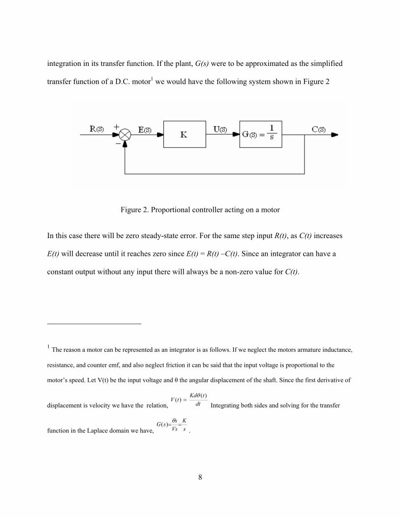
integration in its transfer function. If the plant, G(s) were to be approximated as the simplified

transfer function of a D.C. motor1 we would have the following system shown in Figure 2

Figure 2. Proportional controller acting on a motor

In this case there will be zero steady-state error. For the same step input R(t), as C(t) increases

E(t) will decrease until it reaches zero since E(t) = R(t) –C(t). Since an integrator can have a

constant output without any input there will always be a non-zero value for C(t).

1 The reason a motor can be represented as an integrator is as follows. If we neglect the motors armature inductance,

resistance, and counter emf, and also neglect friction it can be said that the input voltage is proportional to the

motor’s speed. Let V(t) be the input voltage and θ the angular displacement of the shaft. Since the first derivative of

displacement is velocity we have the relation, dttKd

tV)(

)(θ

= Integrating both sides and solving for the transfer

function in the Laplace domain we have, sK

VsssG ==θ)(

.

9

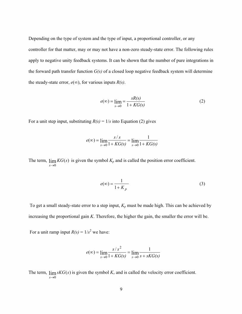
Depending on the type of system and the type of input, a proportional controller, or any

controller for that matter, may or may not have a non-zero steady-state error. The following rules

apply to negative unity feedback systems. It can be shown that the number of pure integrations in

the forward path transfer function G(s) of a closed loop negative feedback system will determine

the steady-state error, e(∞), for various inputs R(s).

KG(s)sR(s)e

s +==∞

→ 1)( lim

0 (2)

For a unit step input, substituting R(s) = 1/s into Equation (2) gives

KG(s)KG(s)sse

ss +=

+=∞

→→ 11

1/)( limlim

00

The term, )(lim0

sKGs→

is given the symbol Kp and is called the position error coefficient.

pKe

+=∞

11)( (3)

To get a small steady-state error to a step input, Kp must be made high. This can be achieved by

increasing the proportional gain K. Therefore, the higher the gain, the smaller the error will be.

For a unit ramp input R(s) = 1/s2 we have:

sKG(s)sKG(s)sse

ss +=

+=∞

→→

11

/)( limlim0

2

0

The term, )(lim0

ssKGs→

is given the symbol Kv and is called the velocity error coefficient.

10

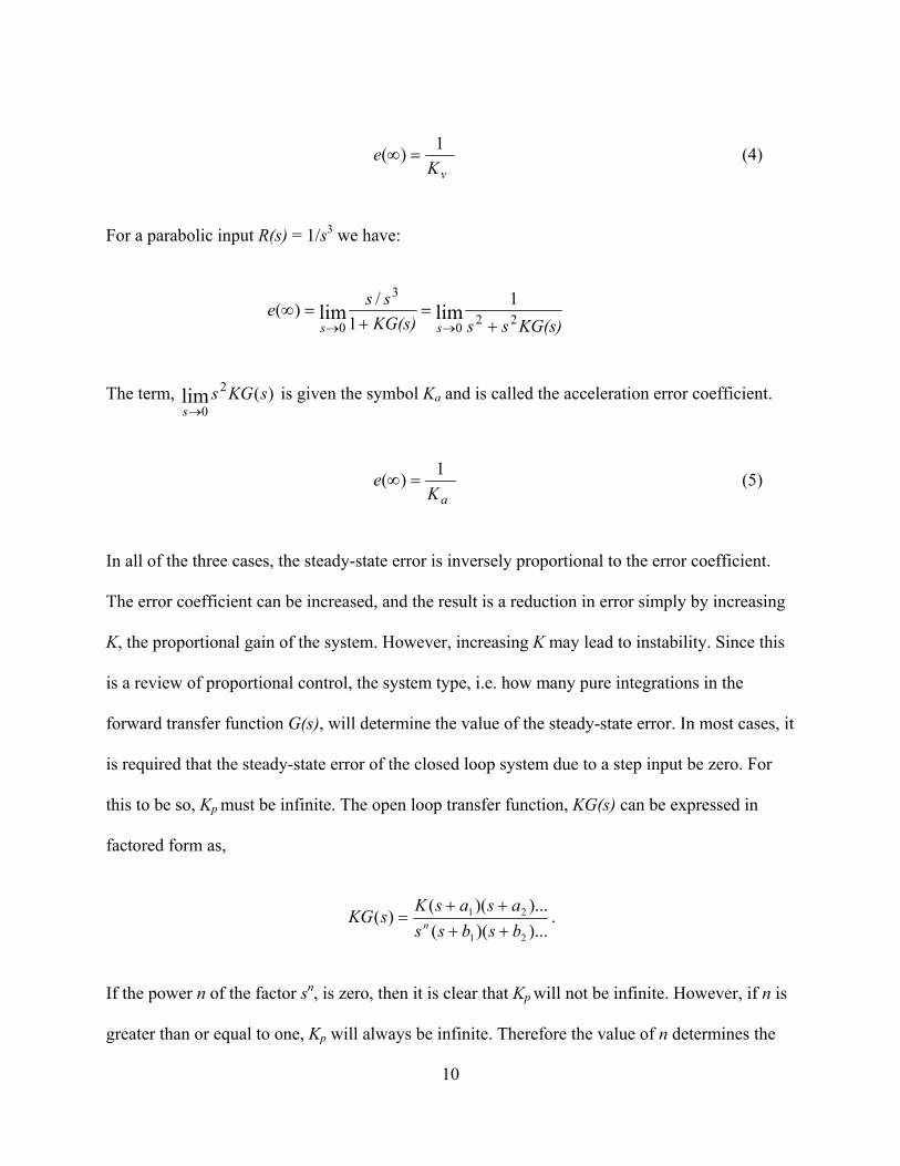
vKe 1)( =∞ (4)

For a parabolic input R(s) = 1/s3 we have:

KG(s)ssKG(s)sse

ss 220

3

0

11

/)( limlim+

=+

=∞→→

The term, )(2

0lim sKGss→

is given the symbol Ka and is called the acceleration error coefficient.

aKe 1)( =∞ (5)

In all of the three cases, the steady-state error is inversely proportional to the error coefficient.

The error coefficient can be increased, and the result is a reduction in error simply by increasing

K, the proportional gain of the system. However, increasing K may lead to instability. Since this

is a review of proportional control, the system type, i.e. how many pure integrations in the

forward transfer function G(s), will determine the value of the steady-state error. In most cases, it

is required that the steady-state error of the closed loop system due to a step input be zero. For

this to be so, Kp must be infinite. The open loop transfer function, KG(s) can be expressed in

factored form as,

)...)(()...)(()(

21

21

bsbssasasKsKG n ++

++= .

If the power n of the factor sn, is zero, then it is clear that Kp will not be infinite. However, if n is

greater than or equal to one, Kp will always be infinite. Therefore the value of n determines the

11

value of the error coefficients, which in turn determine whether the steady-state error equals

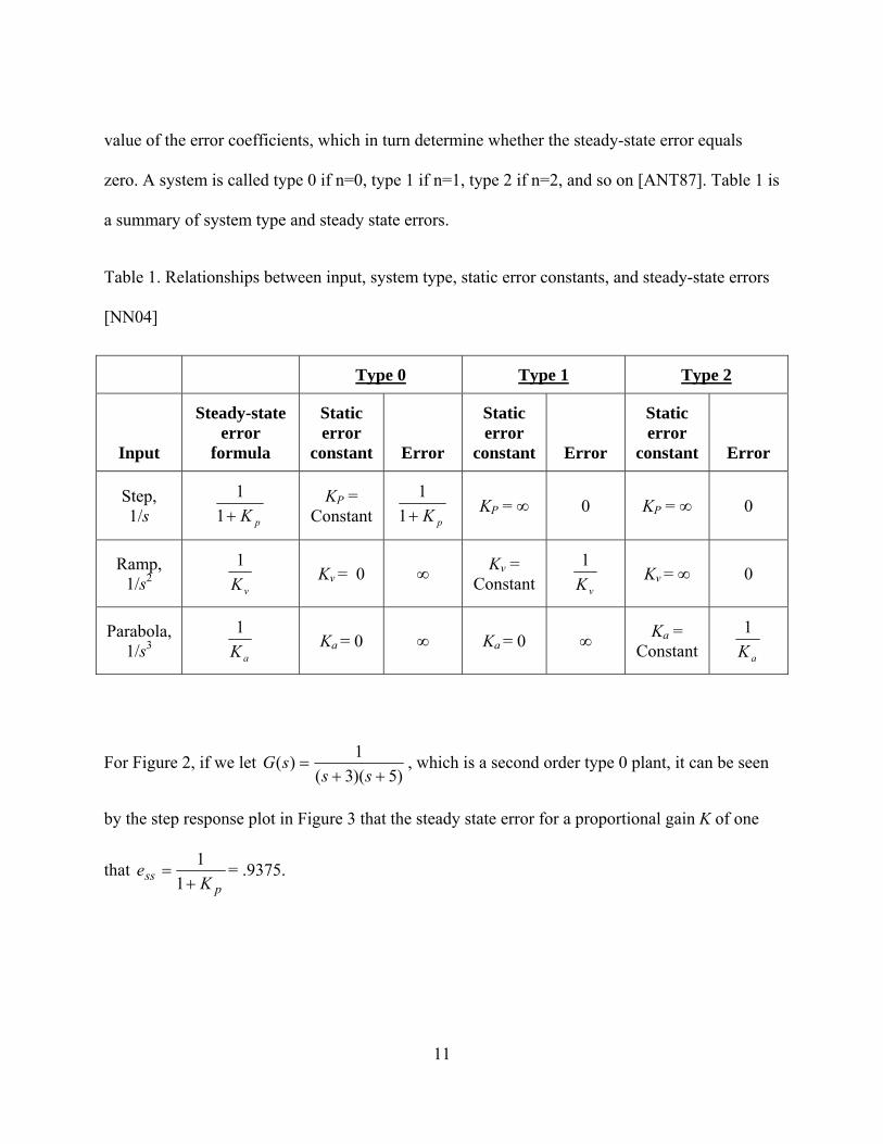
zero. A system is called type 0 if n=0, type 1 if n=1, type 2 if n=2, and so on [ANT87]. Table 1 is

a summary of system type and steady state errors.

Table 1. Relationships between input, system type, static error constants, and steady-state errors

[NN04]

Type 0 Type 1 Type 2

Input

Steady-state error

formula

Static error

constant Error

Static error

constant Error

Static error

constant Error

Step, 1/s pK+1

1 KP = Constant pK+1

1 KP = ∞ 0 KP = ∞ 0

Ramp, 1/s2 vK

1 Kv = 0 ∞ Kv = Constant vK

1 Kv = ∞ 0

Parabola,1/s3 aK

1 Ka = 0 ∞ Ka = 0 ∞ Ka = Constant aK

1

For Figure 2, if we let )5)(3(

1)(++

=ss

sG , which is a second order type 0 plant, it can be seen

by the step response plot in Figure 3 that the steady state error for a proportional gain K of one

that p

ss Ke

+=

11 = .9375.

12

Figure 3. Second order type 0 step response with gain of 1

A plot of the root locus in Figure 4 of the system shows that it will remain stable as the gain K is

increased.

Figure 4. Root locus of second order type 0 system

13

By raising the controller gain to 400 we achieve a steady-state error of .0361. The system

remains stable and the settling time decreases, however we have introduced a certain amount of

overshoot and ringing into the system. Figure 5 depicts the results of a step response to the

system with the gain increased to 400.

Figure 5. Second order type 0 response with gain of 400

If the plant were to be represented as a type 1 third order system with )5)(3(

1)(++

=sss

sG , the

steady state error for a step input will now be zero. Increasing the gain beyond a certain point

will cause instability. By reviewing the root locus plot in Figure 6 we see that when the system

gain is increased to a value greater than 120, the poles of the system will move into the right half

plane and the system will become unstable.

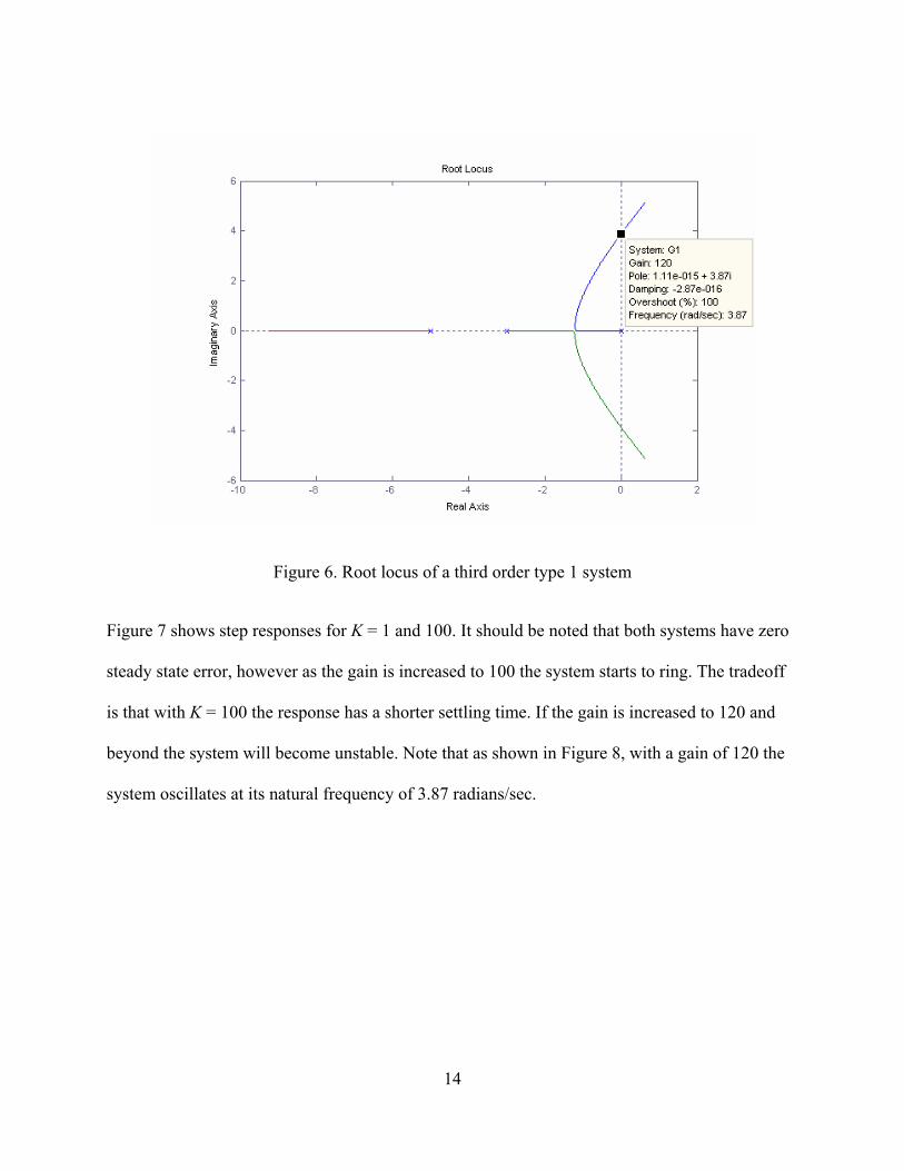
14

Figure 6. Root locus of a third order type 1 system

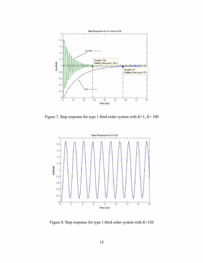
Figure 7 shows step responses for K = 1 and 100. It should be noted that both systems have zero

steady state error, however as the gain is increased to 100 the system starts to ring. The tradeoff

is that with K = 100 the response has a shorter settling time. If the gain is increased to 120 and

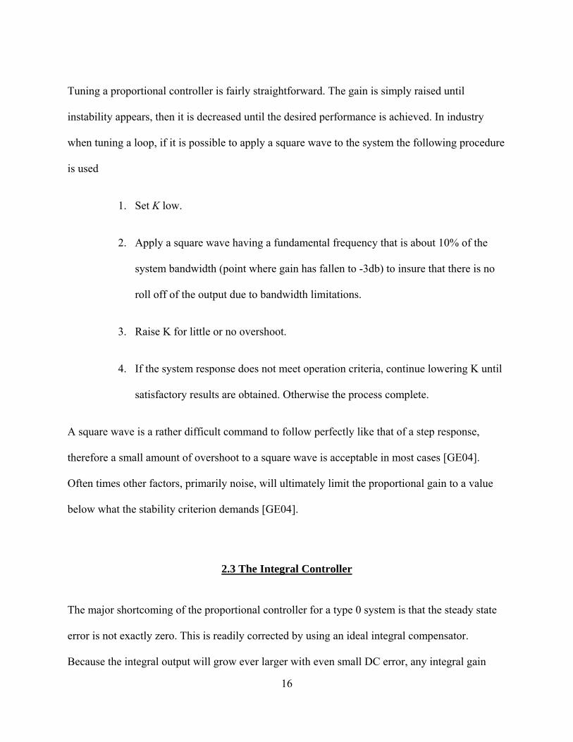
beyond the system will become unstable. Note that as shown in Figure 8, with a gain of 120 the

system oscillates at its natural frequency of 3.87 radians/sec.

15

Figure 7. Step response for type 1 third order system with K=1, K= 100

Figure 8. Step response for type 1 third order system with K=120

16

Tuning a proportional controller is fairly straightforward. The gain is simply raised until

instability appears, then it is decreased until the desired performance is achieved. In industry

when tuning a loop, if it is possible to apply a square wave to the system the following procedure

is used

1. Set K low.

2. Apply a square wave having a fundamental frequency that is about 10% of the

system bandwidth (point where gain has fallen to -3db) to insure that there is no

roll off of the output due to bandwidth limitations.

3. Raise K for little or no overshoot.

4. If the system response does not meet operation criteria, continue lowering K until

satisfactory results are obtained. Otherwise the process complete.

A square wave is a rather difficult command to follow perfectly like that of a step response,

therefore a small amount of overshoot to a square wave is acceptable in most cases [GE04].

Often times other factors, primarily noise, will ultimately limit the proportional gain to a value

below what the stability criterion demands [GE04].

2.3 The Integral Controller

The major shortcoming of the proportional controller for a type 0 system is that the steady state

error is not exactly zero. This is readily corrected by using an ideal integral compensator.

Because the integral output will grow ever larger with even small DC error, any integral gain

17

will eliminate steady-state error. This single advantage is why PI (proportional plus integral)

control is often preferred over P only control [GE04]. A compensator that uses pure integration

to improve steady-state error is referred to as an ideal integral compensator. The ideal

compensator has to be constructed with active components, which in the case of electric

networks requires the use of active amplifiers and sometimes additional power sources. A

passive compensator is less expensive to implement, however in this case the steady-state error is

not driven to zero, where as it is in cases where ideal compensation is used [NN04].

It has been shown in section 2.2 that steady-state error can be removed simply by adding a pure

integration to the controller or plant in a cascaded system. This of course will change the system

type from a type 0 to a type 1. The problem that may arise is that adding this pure integration

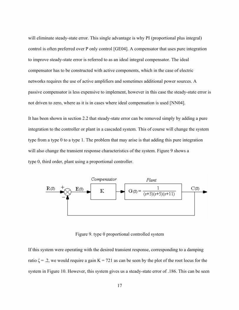
will also change the transient response characteristics of the system. Figure 9 shows a

type 0, third order, plant using a proportional controller.

Figure 9. type 0 proportional controlled system

If this system were operating with the desired transient response, corresponding to a damping

ratio ζ = .2, we would require a gain K = 721 as can be seen by the plot of the root locus for the

system in Figure 10. However, this system gives us a steady-state error of .186. This can be seen

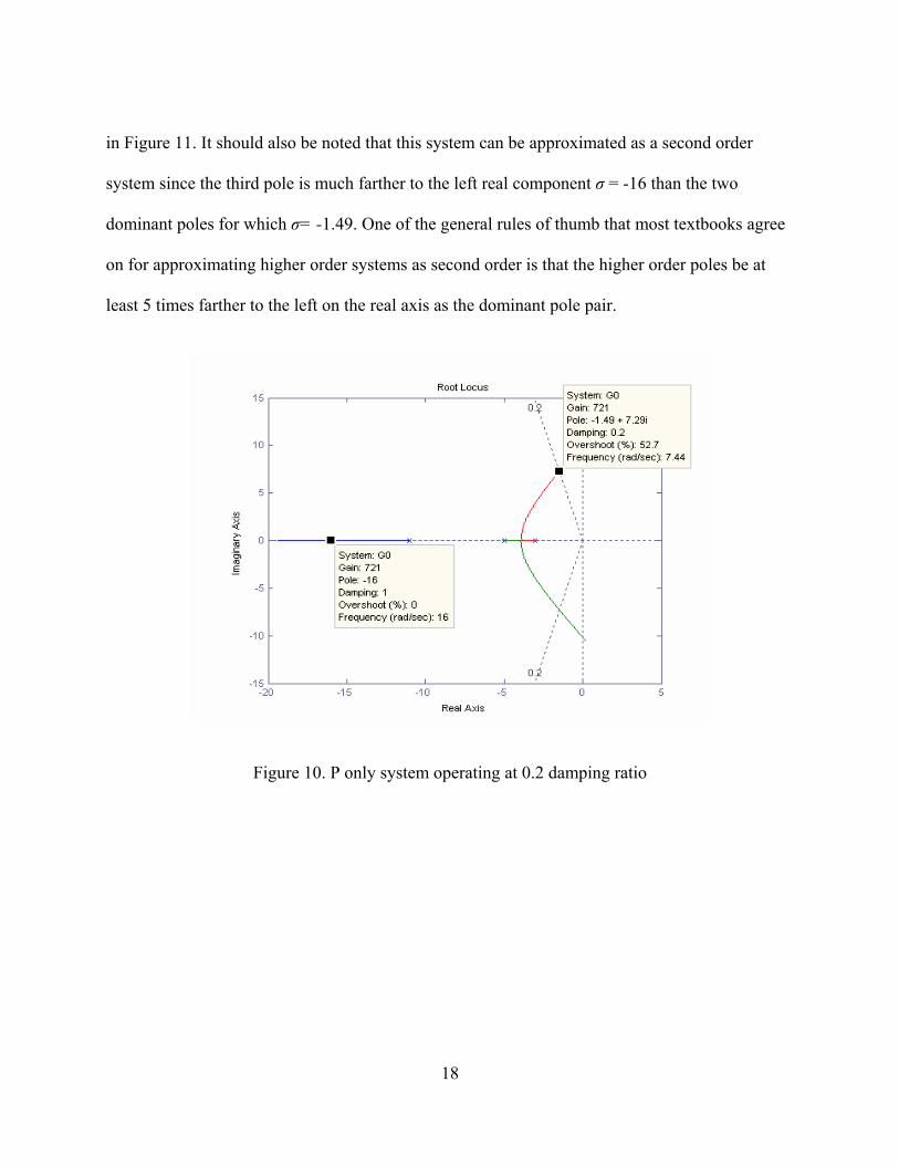
18

in Figure 11. It should also be noted that this system can be approximated as a second order

system since the third pole is much farther to the left real component σ = -16 than the two

dominant poles for which σ= -1.49. One of the general rules of thumb that most textbooks agree

on for approximating higher order systems as second order is that the higher order poles be at

least 5 times farther to the left on the real axis as the dominant pole pair.

Figure 10. P only system operating at 0.2 damping ratio

19

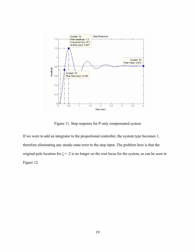
Figure 11. Step response for P only compensated system

If we were to add an integrator to the proportional controller, the system type becomes 1,

therefore eliminating any steady-state error to the step input. The problem here is that the

original pole location for ζ = .2 is no longer on the root locus for the system, as can be seen in

Figure 12.

20

Figure 12. Root locus for PI control with .2 damping ration and no zeros

Analyzing the root locus in Figure 12 it is found that a system gain of 412 will result in a

damping ration ζ = .2. This will give the same percent overshoot as the original system but with

zero steady-state error. However the transient response will be considerably slower i.e. longer

rise time and longer settling time, as seen in Figure 13.

21

Figure 13. Normalized step response for P and PI controller with pure integration and no zero

The system can be made more like the original P only system shown in Figure 11and still

eliminate steady state error by adding a zero to the controller near the origin. The effect of the

zero will help cancel out the angular contribution of the added pole at the origin. This is the final

implementation of an ideal PI controller; one realization of the system is depicted in Figure 14.

Figure 14. Full PI compensator with zero added

22

If parameter a in Figure 14 is chosen to be equal to .2 we have the root locus plot shown in

Figure 15.

Figure 15. Root locus of PI system with zero added

Note that this root locus is extremely close to the original root locus of the proportional only

system. The result is a system with the desired transient response and zero steady-state error to a

step input. This can be seen in the step response plot of Figure 16.

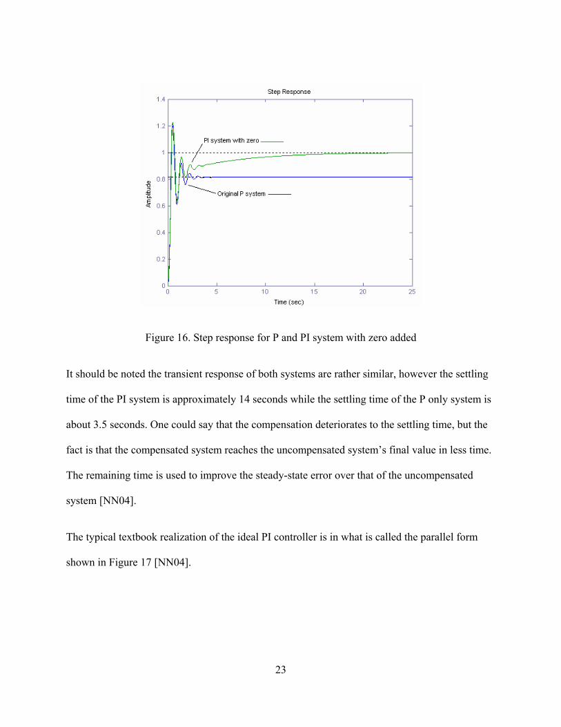
23

Figure 16. Step response for P and PI system with zero added

It should be noted the transient response of both systems are rather similar, however the settling

time of the PI system is approximately 14 seconds while the settling time of the P only system is

about 3.5 seconds. One could say that the compensation deteriorates to the settling time, but the

fact is that the compensated system reaches the uncompensated system’s final value in less time.

The remaining time is used to improve the steady-state error over that of the uncompensated

system [NN04].

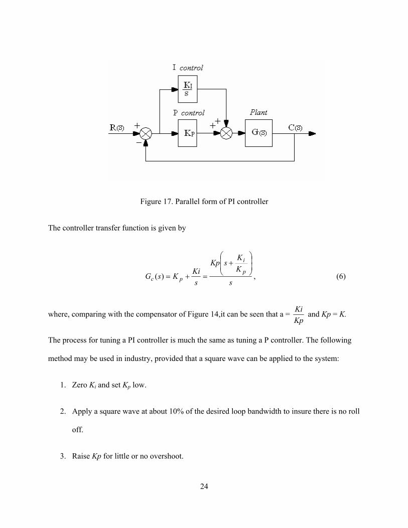
The typical textbook realization of the ideal PI controller is in what is called the parallel form

shown in Figure 17 [NN04].

24

Figure 17. Parallel form of PI controller

The controller transfer function is given by

s

KK

sKp

sKiKsG p

i

pc

⎟⎟⎠

⎞⎜⎜⎝

⎛+

=+=)( , (6)

where, comparing with the compensator of Figure 14,it can be seen that a = KpKi and Kp = K.

The process for tuning a PI controller is much the same as tuning a P controller. The following

method may be used in industry, provided that a square wave can be applied to the system:

1. Zero Ki and set Kp low.

2. Apply a square wave at about 10% of the desired loop bandwidth to insure there is no roll

off.

3. Raise Kp for little or no overshoot.

25

4. If the system response is too noisy, lower Kp until it is not.

5. Raise Ki for 15% overshoot.

2.4 The Derivative Controller

If a system were to already have zero steady-state error, i.e. type 1 or greater, or an acceptable

level of steady-state error, the designer may want to improve the transient response of the

system. The design objective here may be to reduce settling time and achieve a desirable percent

overshoot. This can be accomplished by the use of ideal derivative compensation. The term ideal

refers to the fact that a pure differentiation is applied to the forward path. The ideal proportional

plus derivative PD controller uses active components in its realization, and the pros and cons of

design and manufacturing the system are similar to those of the previous active PI network.

The transient response of a system can be chosen by selecting the required closed-loop pole

locations on the s-plane. If these pole locations are not already on the root locus of the system,

then the system root locus must be reshaped in order to include these poles. One way to

accomplish this is to add a zero to the forward path transfer function.

0)( assGc += (7)

This is the ideal derivative or PD controller and is the sum of a differentiator and a pure gain

[NN04].

26

In the next example the effects of adding zeros at -3, -4 and -6 will be examined on the following

uncompensated plant.

)8)(3)(2(1)(

+++=

ssssG

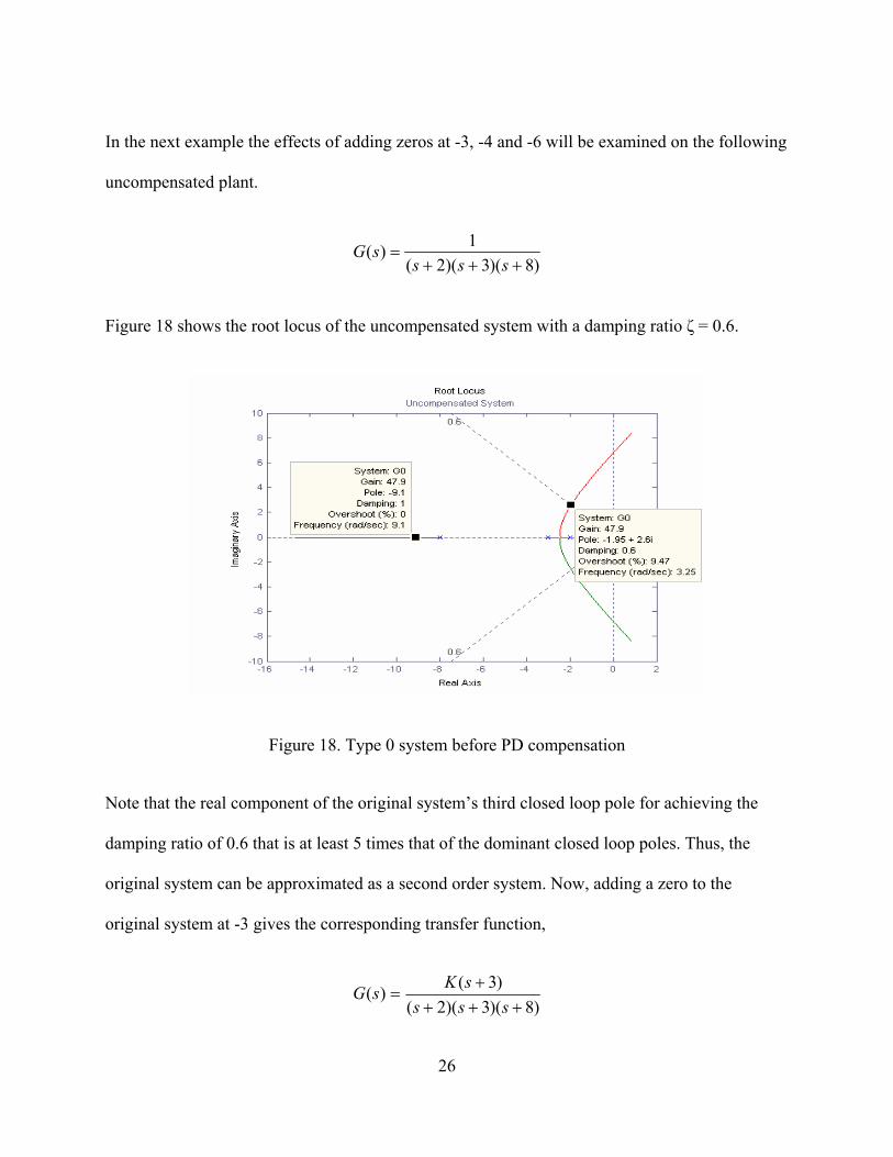
Figure 18 shows the root locus of the uncompensated system with a damping ratio ζ = 0.6.

Figure 18. Type 0 system before PD compensation

Note that the real component of the original system’s third closed loop pole for achieving the

damping ratio of 0.6 that is at least 5 times that of the dominant closed loop poles. Thus, the

original system can be approximated as a second order system. Now, adding a zero to the

original system at -3 gives the corresponding transfer function,

)8)(3)(2()3()(+++

+=

ssssKsG

27

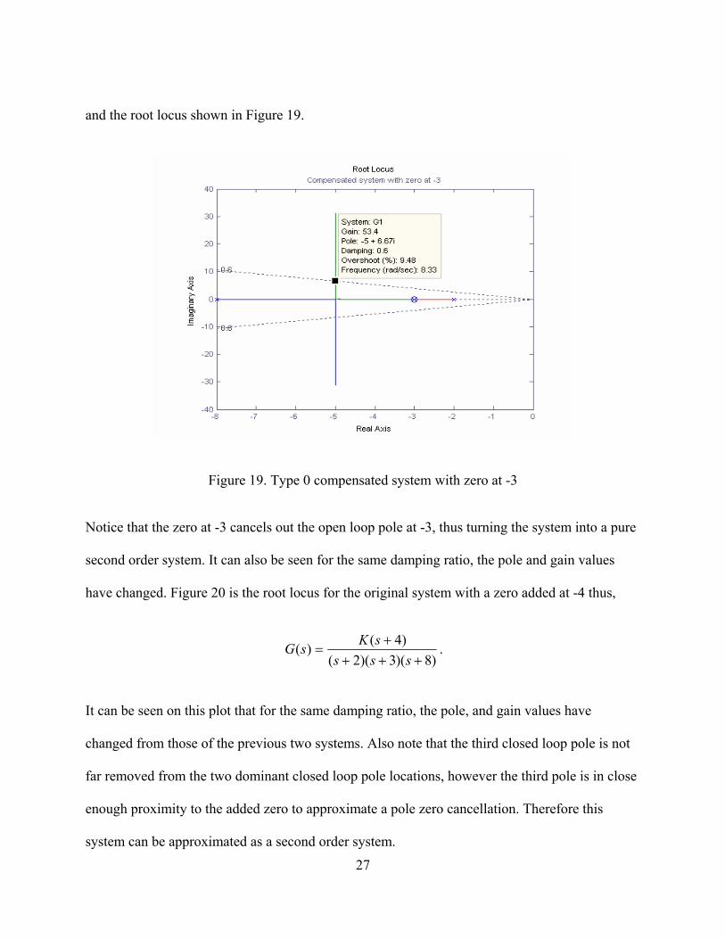
and the root locus shown in Figure 19.

Figure 19. Type 0 compensated system with zero at -3

Notice that the zero at -3 cancels out the open loop pole at -3, thus turning the system into a pure

second order system. It can also be seen for the same damping ratio, the pole and gain values

have changed. Figure 20 is the root locus for the original system with a zero added at -4 thus,

)8)(3)(2()4()(+++

+=

ssssKsG .

It can be seen on this plot that for the same damping ratio, the pole, and gain values have

changed from those of the previous two systems. Also note that the third closed loop pole is not

far removed from the two dominant closed loop pole locations, however the third pole is in close

enough proximity to the added zero to approximate a pole zero cancellation. Therefore this

system can be approximated as a second order system.

28

Figure 20. Type 0 compensated system with zero at -4

In Figure 21 the zero is now moved to -7 giving the transfer function

)8)(3)(2()7()(+++

+=

ssssKsG .

Again it is observed that this system has different pole and gain values for a ζ = 0.6. This system

can also be approximated as a second order system because of the fact that the zero is fairly far

removed from the dominate pole pair and it is also in close proximity to the third pole, offering a

rough approximation of pole zero cancellation.

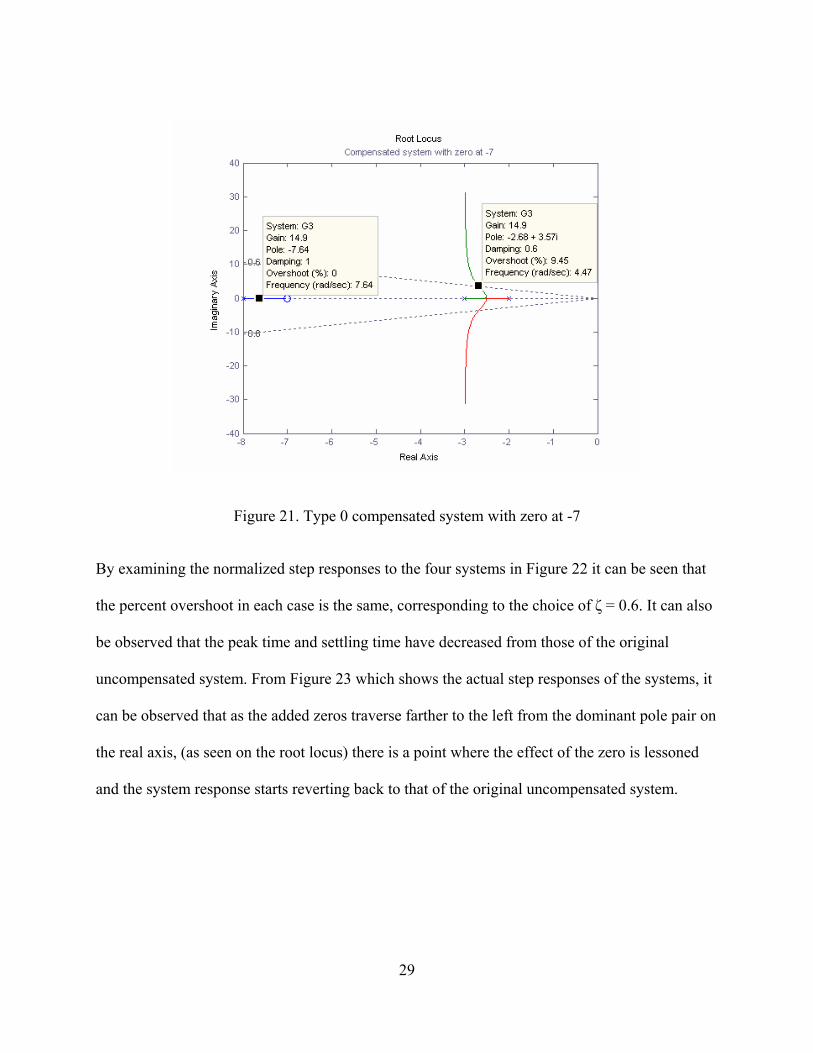
29

Figure 21. Type 0 compensated system with zero at -7

By examining the normalized step responses to the four systems in Figure 22 it can be seen that

the percent overshoot in each case is the same, corresponding to the choice of ζ = 0.6. It can also

be observed that the peak time and settling time have decreased from those of the original

uncompensated system. From Figure 23 which shows the actual step responses of the systems, it

can be observed that as the added zeros traverse farther to the left from the dominant pole pair on

the real axis, (as seen on the root locus) there is a point where the effect of the zero is lessoned

and the system response starts reverting back to that of the original uncompensated system.

30

Figure 22. Normalized step responses for uncompensated and derivative compensated systems

Figure 23. Step responses for uncompensated and derivative compensated systems

31

It can be seen that the step responses for the systems with a zero at -3 and -4 give the most

improvement to transient response and steady-state error therefore, it is important to make a

judicious choice when selecting the zero location.

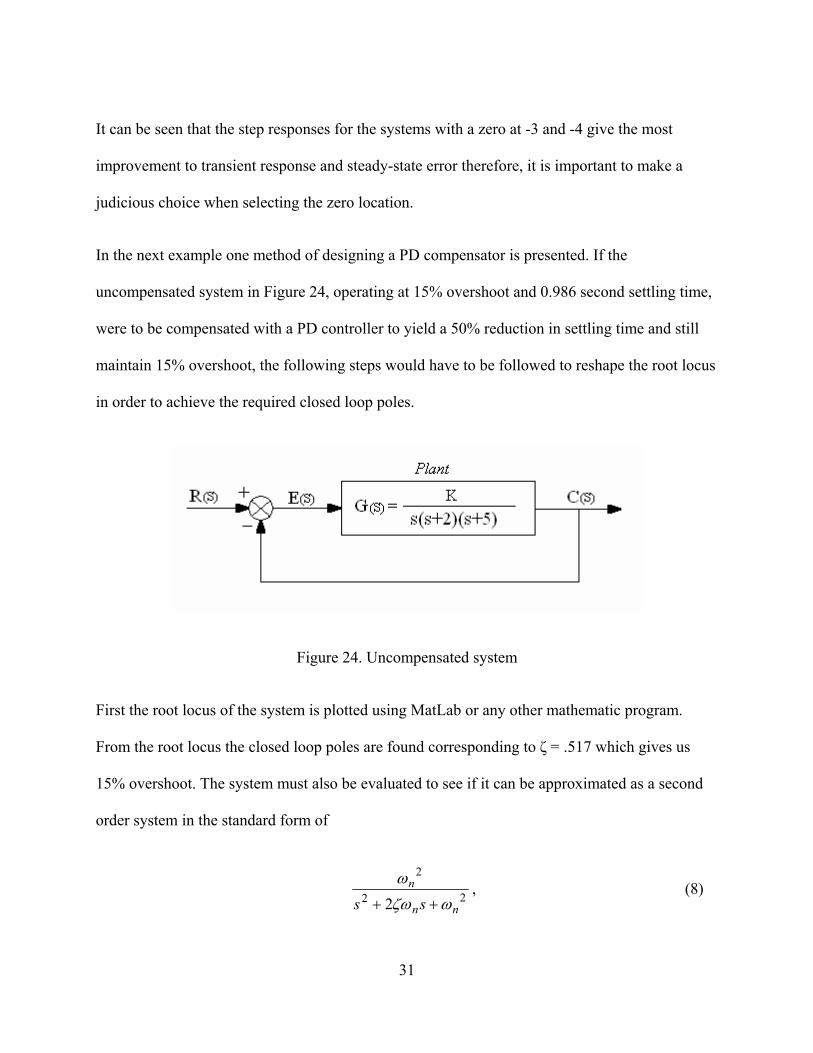
In the next example one method of designing a PD compensator is presented. If the

uncompensated system in Figure 24, operating at 15% overshoot and 0.986 second settling time,

were to be compensated with a PD controller to yield a 50% reduction in settling time and still

maintain 15% overshoot, the following steps would have to be followed to reshape the root locus

in order to achieve the required closed loop poles.

Figure 24. Uncompensated system

First the root locus of the system is plotted using MatLab or any other mathematic program.

From the root locus the closed loop poles are found corresponding to ζ = .517 which gives us

15% overshoot. The system must also be evaluated to see if it can be approximated as a second

order system in the standard form of

22

2

2 nn

n

ss ωζω

ω

++, (8)

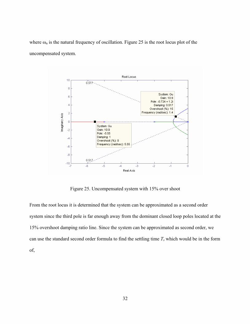
32

where ωn is the natural frequency of oscillation. Figure 25 is the root locus plot of the

uncompensated system.

Figure 25. Uncompensated system with 15% over shoot

From the root locus it is determined that the system can be approximated as a second order

system since the third pole is far enough away from the dominant closed loop poles located at the

15% overshoot damping ratio line. Since the system can be approximated as second order, we

can use the standard second order formula to find the settling time Ts which would be in the form

of,

33

σζω44

==n

sT (9)

where σ is the real part of the closed loop dominant pole obtained from the root locus. Ts of the

uncompensated system is found to be 5.5 seconds. To achieve a settling time of 2.7 seconds the

new compensated σ would have to equal -1.448. To find the imaginary part of the compensated

pole location ωd we use simple trigonometry to find that,

))(tan(cos 1 ςσω −=d (10)

therefore,

4.2)86.58tan(448.1 =°=dω .

The angle 58.86о corresponds to ζ = 0.517. The required new closed loop pole location for a 15%

over shoot and the decreased settling time of 2.763 seconds is

4.2448.1 j±− .

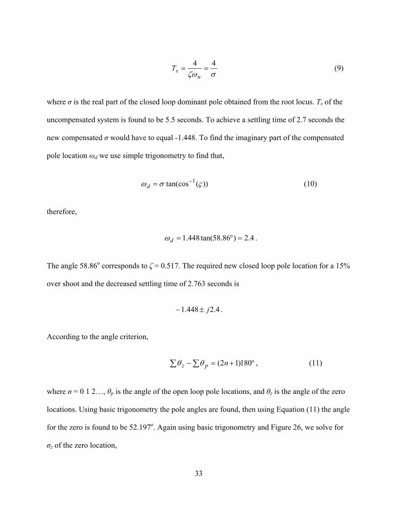
According to the angle criterion,

°+=−∑ ∑ 180)12( npz θθ , (11)

where n = 0 1 2…, θp is the angle of the open loop pole locations, and θz is the angle of the zero

locations. Using basic trigonometry the pole angles are found, then using Equation (11) the angle

for the zero is found to be 52.197о. Again using basic trigonometry and Figure 26, we solve for

σz of the zero location,

34

)tan( zz

d θσσ

ω=

−, (12)

thus,

)197.52tan(448.1

4.2°=

−σ.

The value of σ is found to be -3.310.

Figure 26. Required pole location for compensation

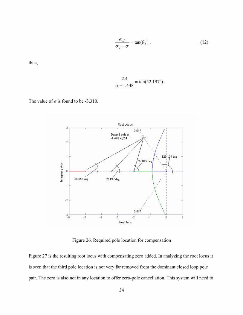
Figure 27 is the resulting root locus with compensating zero added. In analyzing the root locus it

is seen that the third pole location is not very far removed from the dominant closed loop pole

pair. The zero is also not in any location to offer zero-pole cancellation. This system will need to

35

be simulated to see if a second order approximation is valid. Figure 28 is plot of the step

responses for the uncompensated and compensated systems.

Figure 27. Derivative compensated system root locus

36

Figure 28. Step response for uncompensated and derivative compensated system

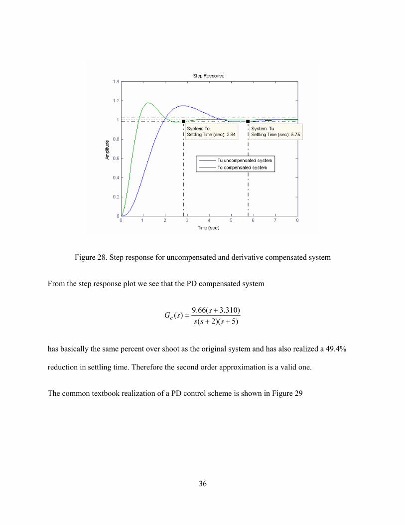
From the step response plot we see that the PD compensated system

)5)(2()310.3(66.9)(

+++

=sss

ssGc

has basically the same percent over shoot as the original system and has also realized a 49.4%

reduction in settling time. Therefore the second order approximation is a valid one.

The common textbook realization of a PD control scheme is shown in Figure 29

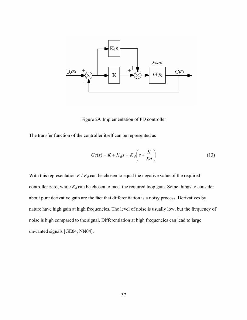
37

Figure 29. Implementation of PD controller

The transfer function of the controller itself can be represented as

⎟⎠⎞

⎜⎝⎛ +=+=

KdKsKsKKsGc dd)( (13)

With this representation K / Kd can be chosen to equal the negative value of the required

controller zero, while Kd can be chosen to meet the required loop gain. Some things to consider

about pure derivative gain are the fact that differentiation is a noisy process. Derivatives by

nature have high gain at high frequencies. The level of noise is usually low, but the frequency of

noise is high compared to the signal. Differentiation at high frequencies can lead to large

unwanted signals [GE04, NN04].

38

2.5 The Proportional Integral Derivative Controller

A system that can be used to improve steady-state error as well as transient response is known as

the proportional integral derivative controller or PID controller. The mathematical or ideal

textbook configuration of the system can be seen in Figure 30.

Figure 30. Ideal PID representation

The controller transfer function can be represented as

sKK

sKK

sK

ssKKsK

sKs

KKsG c

b

c

ac

cbac

bac

⎟⎟⎠

⎞⎜⎜⎝

⎛++

=++

=++=

22

)( . (14)

Notice that this controller has one pole at the origin and two zeros. From the review for PI and

PD controllers it can be seen that one of the zeros and the pole at the origin will pertain to the

ideal integral compensator, and the remaining zero will be used to design in the ideal derivative

compensator [NN04].

39

The following process can be used to design a PID system. Choosing the example plant transfer

function

)9)(4)(2()8.7()(+++

+=

sssssG p ,

and the operating criteria that the uncompensated system operating at 25% overshoot is to be

improved to have a 30% reduction in settling time and zero steady-state error, while maintaining

25% overshoot. The root locus of the system is plotted and the closed loop pole for 25% over

shoot is determined. As shown in Figure 31, the third pole and zero are found to be a little closer

than we would like from the dominant poles to evaluate the system as if it were second order. A

simulation was performed and it was found that the second order approximation is still

sufficiently valid for us to proceed. Next we find the compensator pole that will yield the 30%

reduction in settling time and still maintain 25% over shoot. Using Equation (9) the settling time

Ts of the uncompensated system is found to be 1.166 seconds; through simulation, the settling

time was actually .986 seconds which is sufficiently close for this demonstration. The new

required settling time is .816 seconds, using the calculated value of settling time. The real part of

the new pole location is σ = -4.902.

40

Figure 31. System before PID implementation

Again using Equation (10), ωd is found to equal 11.133. The new closed loop poles for 25%

overshoot and a reduced settling time of 0.816 seconds are

133.11902.4 j±− .

Finding the pole and zero angles and using Equation (11) to solve for θz we have θz = 13.62о.

Using Equation (12) the compensator zero location is found to be -50.833.

41

The root locus of the compensated system,

)9)(4)(2()833.50)(8.7()(

+++++

=sss

ssKsG

is plotted and it can be seen that a second order approximation is still questionable. A simulated

step response is applied to the system and it can be seen that the first part of the design goal has

been accomplished. The percent over shoot remains at 25% while the settling time has decreased

from .986 second to .671 seconds, which is a 31% reduction in settling time. Figure 32 is the new

root locus, while Figure 33 gives step responses for the original and compensated systems.

Figure 32. Root locus of derivative compensated system

42

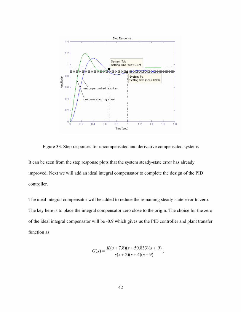
Figure 33. Step responses for uncompensated and derivative compensated systems

It can be seen from the step response plots that the system steady-state error has already

improved. Next we will add an ideal integral compensator to complete the design of the PID

controller.

The ideal integral compensator will be added to reduce the remaining steady-state error to zero.

The key here is to place the integral compensator zero close to the origin. The choice for the zero

of the ideal integral compensator will be -0.9 which gives us the PID controller and plant transfer

function as

)9)(4)(2()9.)(833.50)(8.7()(

++++++

=ssss

sssKsG ,

43

where K is equal to 1.9. Figures 34 and 35 show the root locus plot for the PID system and the

corresponding step responses. Notice that the root locus for the PID system now has four closed

loop poles. The step response shows that while the ideal derivative compensator decreased the

settling time by the desired amount and also lowered the steady state error, the PID compensator

brought the steady-state error two zero, however the settling time increased from that of the

derivative compensation, yet was still an improvement from that of the uncompensated system.

Figure 34. PID compensated root locus

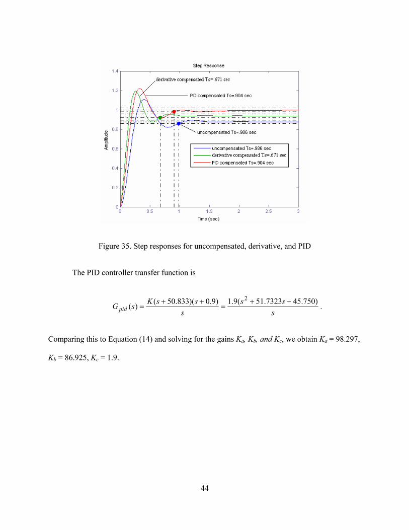
44

Figure 35. Step responses for uncompensated, derivative, and PID

The PID controller transfer function is

sss

sssKsG pid

)750.457323.51(9.1)9.0)(833.50()(2 ++

=++

= .

Comparing this to Equation (14) and solving for the gains Ka, Kb, and Kc, we obtain Ka = 98.297,

Kb = 86.925, Kc = 1.9.

45

2.6 Conclusion

In this chapter a review of all the components that make up a PID controller was made along

with a review of some basic definitions. It should be noted that all of the systems were linear and

time invariant, because that is what the PID algorithm is best suited for.

It was shown that proportional control alone with a type 0 plant will always have a steady-state

error. An example of a third order type 1 system was also given to demonstrate that it is possible

to choose a gain that is too high, thus introducing ringing and instability to a system. The

addition of PI control was made to bring the steady-state error to zero; with proper zero

placement it does not change the transient response of a system by a considerable amount. The

PD controller was demonstrated to improve transient response, while also offering a small

amount of steady-state error improvement. It can be seen that the design process for a PD control

scheme is rather involved as compared to that of a PI system. Derivative compensation and

tuning is not a straight-forward task. The PID controller was realized in what is commonly

called the text book, or ideal version. The design example revealed that while the first part of the

design, which implemented the ideal derivative compensation, was a success, the further addition

of the ideal integral compensation eliminated the steady-state error but also took away from

some of the improvement of transient response from the ideal derivative compensation. There

was however an overall improvement of steady-state and transient response over that of the

original uncompensated system. This is part of the motivation behind this paper. The fact is that

the PID algorithm is interactive, and changing one gain parameter affects the response of the

whole system.

46

CHAPTER 3: STANDARD PID TUNING METHODS

3.1 Introduction

This chapter will present the evaluation of various tuning methods. In section 3.2 we will discuss

the various forms of the PID algorithm used in industry. The three most prevalent forms will be

examined. In section 3.3 we will introduce the Step Response or Open Loop method of tuning.

Section 3.4 will be devoted to the Closed Loop or Frequency Response method of tuning. Both

the Open Loop and Closed Loop methods were developed by J.G. Ziegler and N.B. Nichols in

1942 and 1943. In section 3.5 the Chien, Hrones and Reswick (CHR) tuning method will be

demonstrated. This method is supposedly an improvement on the Open Loop method. Lastly

section 3.6 will introduce the so-called Rule of Thumb tuning method. This method is so named

because it is basically a word of mouth method.

3.2 Forms of the PID Algorithm

As stated earlier there is no single PID algorithm used in industry. Different controller

manufacturers use different algorithms. It is extremely important for the control engineer or

technician responsible for tuning a control loop to understand the algorithm used. There are

several PID algorithms, however there are three standard ones.

Recalling that Figure 30 depicted the ideal or textbook example of the PID structure, whose

transfer function was given in Equation (14), we demonstrated in Chapter 2 how different values

47

of Ka, Kb, and Kc can be chosen to accomplish a certain response. The fact is that this is what is

taught in most undergraduate classes; however this first type of representation which will be

referred to as Style I, is usually realized by most manufacturers as,

⎟⎟⎠

⎞⎜⎜⎝

⎛++ ∫

t

di dt

tdeTdeT

teK0

)()(1)( ττ , (15)

where )()()( tctrte −= .

The corresponding transfer function is,

⎟⎟⎠

⎞⎜⎜⎝

⎛++= d

isT

sTKsGc 11)( . (16)

This industrial form is commonly referred to as non-interacting, standard, ideal, or ISA form. Ti

is defined as the integral time, Td is defined as the derivative time, and K is defined as the

controller gain. If we relate the terms in Equation (16) to those of Equation (14) we get K=Ka,

Ti=Ka/Kb, and Td=Kc/Ka. The term non-interacting refers to the fact that the integral time does

not affect the derivative time and visa versa.

The second industrial form of the PID algorithm can be seen in the block diagram of Figure 36.

48

Figure 36. Style II PID block diagram

This controller is commonly referred to as the interacting, series, or classical form. The transfer

function for the Style II controller can be represented as

( )di

c sTsT

KsG '1'

11')(' +⎟⎟⎠

⎞⎜⎜⎝

⎛+= . (17)

The term interacting refers to the fact the changing the derivative term influences the integral

part. The reason that this system is also referred to as classical is that early pneumatic controls

that were used to implement PID control took this mathematical representation. The Style II

interactive controller can be represented as the non-interactive Style I controller by making the

following substitutions [AH95]:

49

i

diT

TTKK

'''

'+

=

dii TTT '' += (18)

di

diTTTT

Td''''

+=

Likewise the non-interactive controller can be represented as the interactive controller by making

the following substitutions:

( )id TTKK /4112

' −+=

( )idi

i TTT

T /4112

' −+= (19)

( )idi

d TTT

T /4112

' −−=

where

di TT 4≥ .

This is why it is so important for the engineer responsible for tuning a system to know the exact

form of the algorithm implemented in the controller. It is worth mentioning that if we expand the

Style II equation we get

50

⎟⎟⎠

⎞⎜⎜⎝

⎛+++=

i

d

idc T

TsT

sTKsG''

'1'1')(

therefore if we implement a P only, PI only, or PD only control scheme both Style I and Style II

forms are equivalent. The third most common form referred to as Style III is the parallel form. Its

transfer function is

di sk

sK

ksG ++=)('' (20)

The parameters of the parallel form are related to the standard Style I form by the following

relations [AH95]:

Kk =

i

i TKk = (21)

dd KTk =

It should be noted that some control manufacturers refer to the integral time as 1/ki, which could

be very confusing when trying to tune a controller.

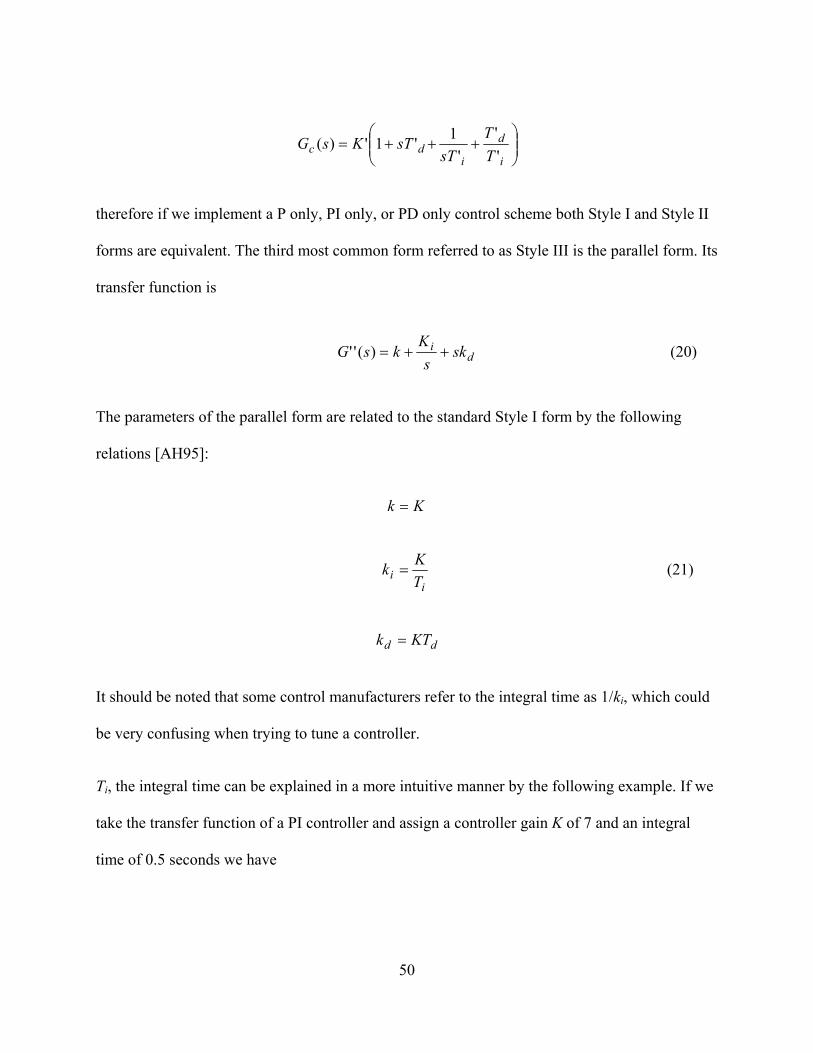
Ti, the integral time can be explained in a more intuitive manner by the following example. If we

take the transfer function of a PI controller and assign a controller gain K of 7 and an integral

time of 0.5 seconds we have

51

⎟⎠⎞

⎜⎝⎛ +=⎟⎟

⎠

⎞⎜⎜⎝

⎛+=

ssTKsG

i 5.011711)( .

If we apply a step input to this we get the controller output shown in Figure 37.

Figure 37. Ti intuitively explained

It can be shown that the initial change to the step input is due to the proportional action which

gives us a change of 7 or A in the amplitude of the controller output. The integral time Ti is the

time it takes for the controller output to change the same amount A that was imposed by the

original proportional control. Of course this is not exactly true. When we apply this system to the

plant and close the loop we do not get exactly these results. However, it is good enough to give

an intuitive feel to the system. Ti usually has the units of seconds or minutes per repeat or is

simply called the reset rate. When using a Style I controller we have 1/Ti which is

52

repeats/second, therefore the smaller Ti, the faster the system response is. If we make Ti infinite

we essentially eliminate integral control.

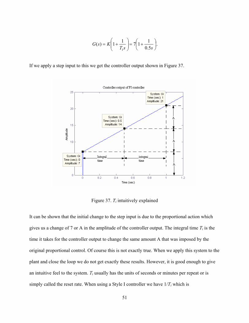
Td, the derivative time can be described as the predictive or pre-actuation time. If we take the PD

controller transfer function with gain K = 2 and Td = 0.05 we have

( ) ( )ssTKsG d 05.0121)( +=+=

By taking the error curve and superimposing the derivative controller on it we get the result

shown in Figure 38.

Figure 38. PD control acting on the error curve

This is of course approximately what happens, but it gives a more intuitive feel for the derivative

time. The action of the PD controller is proportional to the predicted process output, where the

53

prediction is made by extrapolating the error by the tangent to the error curve [AH95]. This is

why we will see from the tuning rules that the derivative time is usually made rather small so as

not to have the prediction veer too far from the actual error.

Chapter two showed the results of varying the gain K of a proportional system. Here since we

have introduced two new terms for the PI and PD controller, namely Ti and Td, we will

demonstrate the effects of varying these terms on a control system operating on a simple plant.

Take the plant transfer function 2)1(1)(+

=s

sG if we apply a PI control to this system with a

gain of K=1 and vary Ti we get the responses to a step input shown in Figure 39.

Figure 39. PI controller with Ti varied

54

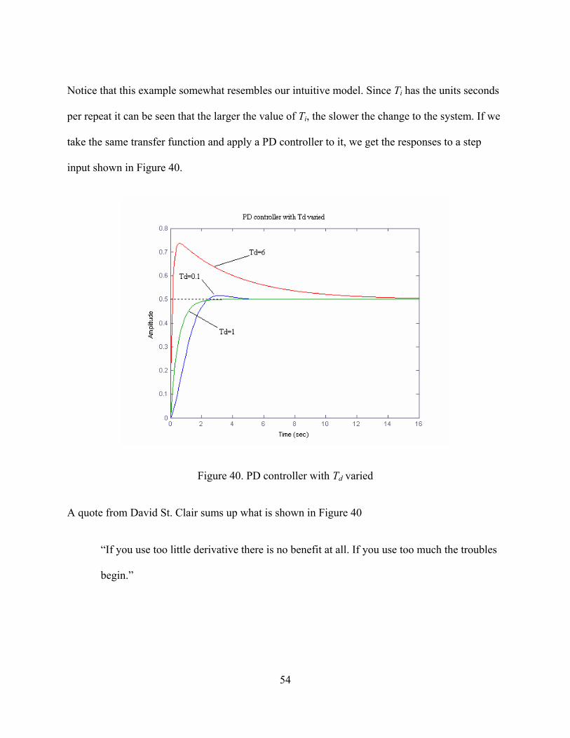
Notice that this example somewhat resembles our intuitive model. Since Ti has the units seconds

per repeat it can be seen that the larger the value of Ti, the slower the change to the system. If we

take the same transfer function and apply a PD controller to it, we get the responses to a step

input shown in Figure 40.

Figure 40. PD controller with Td varied

A quote from David St. Clair sums up what is shown in Figure 40

“If you use too little derivative there is no benefit at all. If you use too much the troubles

begin.”

55

It should be noted that with a Td of 0.1 the response of the system is almost the same as that of

the open loop step response of the system without any control. With Td =6 the system has an

over-predictive nature such as what was shown in our intuitive example.

To reiterate, in this section there are basically three forms of the industrial implementation of the

PID algorithm, which we have defined as Style I, Style II, and Style III. It is extremely important

for the engineers responsible for tuning a control loop to know which form their controller is

implementing before adjusting any of the control parameters available. The tuning rules that

follow are all based on the Style I controller. To implement the results on a different style

controller the engineer must remember to use the conversion formulas previously shown, or the

results could be undesirable or even catastrophic.

3.3 The Open Loop Tuning Method

In 1942 J.G Ziegler and N.B. Nichols derived their first method of PID tuning through empirical

testing. This method was based on the plant reaction to a step input and characterized by two

parameters. The method is often referred to as the Open Loop, or Step Response tuning method.

The parameters, a and L, are determined by applying a unit step function to the process.

56

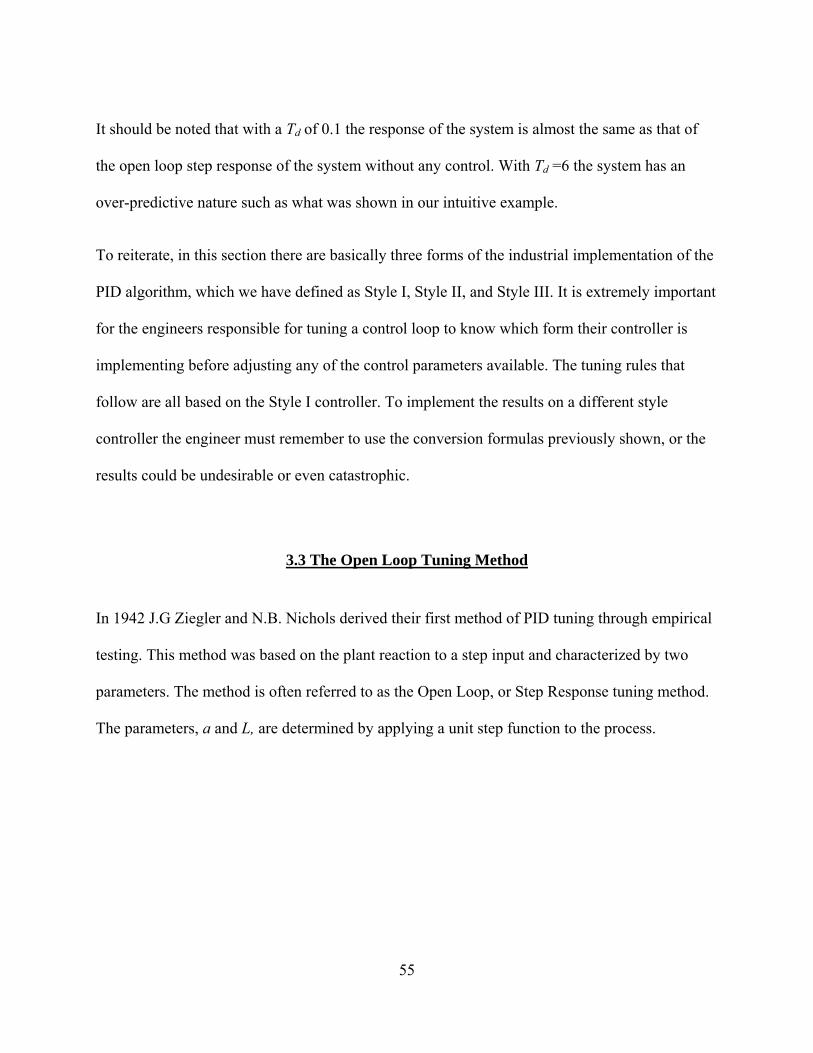
Figure 41. Open loop parameter identification

The original process model that Ziegler and Nichols used was of the form

sLesbsG −=)( .

This is a process with an integrator and a time delay, where b=a/L. Referring to Figure 41, the

point where the slope of the step response has its maximum is first determined, then the tangent

at this point is drawn. The intersection of this tangent and vertical axis at T=0 gives the

parameters a and L. Ziegler and Nichols derived PID parameters as well as P only and PI only,

directly as functions of a and L. The results are given in Table 2.

57

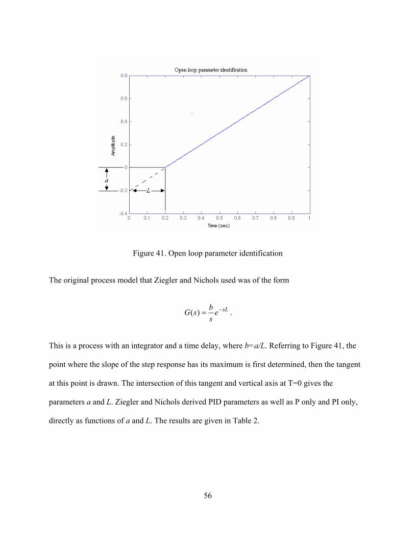
Table 2. Z-N open loop tuning parameters

Controller K Ti Td

P 1/a

PI 0.9/a 3L

PID 1.2/a 2L L/2

We will now demonstrate the Open Loop tuning method on the plant modeled as

3)1(1)(+

=s

sG . From the open loop step response shown in Figure 42 we see that a=0.22 and

L=0.81. Substituting these values in to Table 2 we obtain the PID controller values of K=5.45,

Ti=1.62, and Td=0.405.The resulting controller transfer function is

⎟⎠⎞

⎜⎝⎛ ++= s

ssGc 405.0

62.11145.5)( . Utilizing this controller with our sample plant and applying a

step input we get the results displayed in Figure 43. Notice that the decay ratio d, which is

defined as the ratio between two consecutive maxima of the error for a step change in set point,

is approximately ¼ this is what Ziegler and Nichols strived for in their implementation of the

tuning rules.

58

Figure 42. Z-N open loop parameter evaluation for sample system

Figure 43. Step response for a system tuned using the open loop method

59

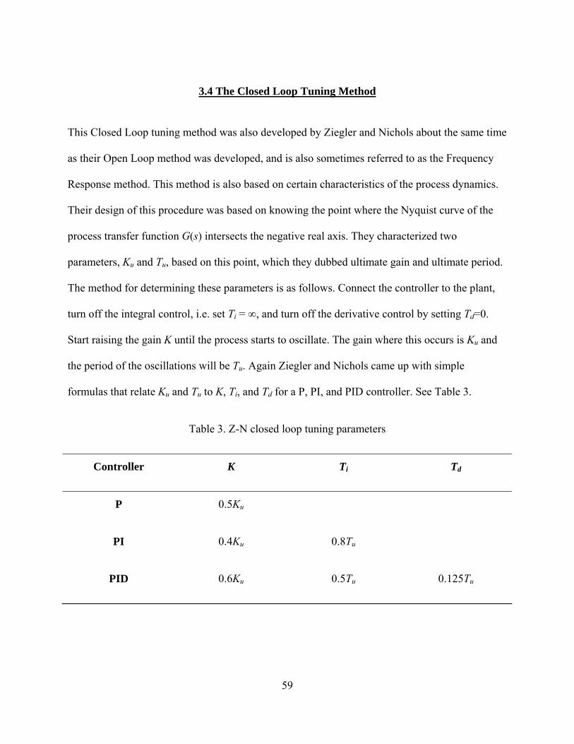
3.4 The Closed Loop Tuning Method

This Closed Loop tuning method was also developed by Ziegler and Nichols about the same time

as their Open Loop method was developed, and is also sometimes referred to as the Frequency

Response method. This method is also based on certain characteristics of the process dynamics.

Their design of this procedure was based on knowing the point where the Nyquist curve of the

process transfer function G(s) intersects the negative real axis. They characterized two

parameters, Ku and Tu, based on this point, which they dubbed ultimate gain and ultimate period.

The method for determining these parameters is as follows. Connect the controller to the plant,

turn off the integral control, i.e. set Ti = ∞, and turn off the derivative control by setting Td=0.

Start raising the gain K until the process starts to oscillate. The gain where this occurs is Ku and

the period of the oscillations will be Tu. Again Ziegler and Nichols came up with simple

formulas that relate Ku and Tu to K, Ti, and Td for a P, PI, and PID controller. See Table 3.

Table 3. Z-N closed loop tuning parameters

Controller K Ti Td

P 0.5Ku

PI 0.4Ku 0.8Tu

PID 0.6Ku 0.5Tu 0.125Tu

60

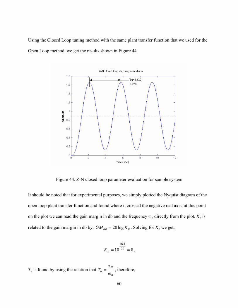
Using the Closed Loop tuning method with the same plant transfer function that we used for the

Open Loop method, we get the results shown in Figure 44.

Figure 44. Z-N closed loop parameter evaluation for sample system

It should be noted that for experimental purposes, we simply plotted the Nyquist diagram of the

open loop plant transfer function and found where it crossed the negative real axis, at this point

on the plot we can read the gain margin in db and the frequency ωn directly from the plot. Ku is

related to the gain margin in db by, udb KGM log20= . Solving for Ku we get,

810 201.18

==uK .

Tu is found by using the relation that n

uTωπ2

= , therefore,

61

632.373.1

2==

πTu .

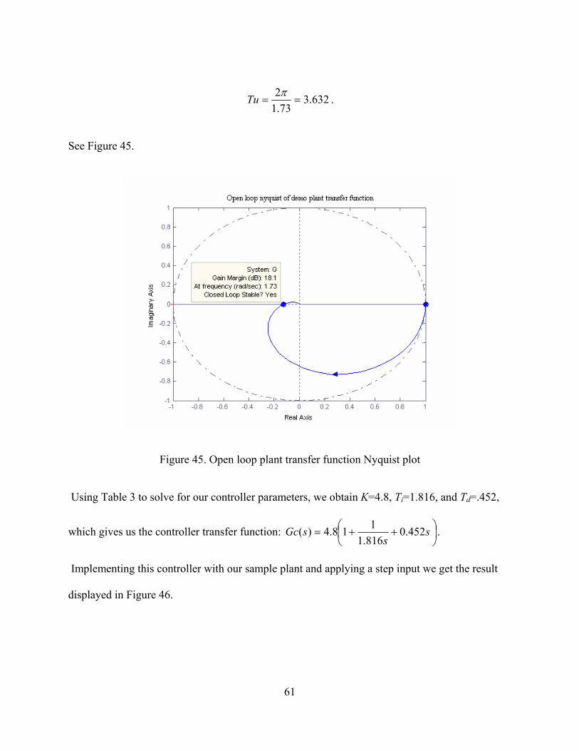
See Figure 45.

Figure 45. Open loop plant transfer function Nyquist plot

Using Table 3 to solve for our controller parameters, we obtain K=4.8, Ti=1.816, and Td=.452,

which gives us the controller transfer function: ⎟⎠⎞

⎜⎝⎛ ++= s

ssGc 452.0

816.1118.4)( .

Implementing this controller with our sample plant and applying a step input we get the result

displayed in Figure 46.

62

Figure 46. Step response for a system tuned using the closed loop method

It can be observed that the Open Loop method allowed for a little more over shoot and a longer

settling time than that of the Closed Loop tuning method. It is obvious that the Ziegler and

Nichols open and closed loop tuning rules are simple to follow. Their original design criteria for

a decay ratio d=0.25, which when applied to a second order model of the form originally shown

in Equation 8 in Chapter 2 ⎟⎟⎠

⎞⎜⎜⎝

⎛

++ 22

2

2 nn

n

ss ωζω

ω, gives us [AH95]

21/2 ζπζ −−= ed . (22)

Setting d=0.25 and solving for the damping ratio we get ζ=.23, which accounts for the rather

large percent overshoot exhibited by the Open and Closed Loop tuning methods. It is also worth

63

mentioning that the Closed Loop terms Ku and Tu are more accurately measured through

empirical means than the Open Loop parameters L and a.

3.5 The Chien, Hrones and Reswick Tuning Method

The Chien, Hrones, and Reswick (CHR) method of tuning was derived from the original

Ziegler-Nichols Open Loop method with the intention of obtaining the quickest response without

overshoot and quickest response with 20% overshoot. To tune the controller according to the

CHR method, the parameters a, L, and T (the time constant of the of the plant transfer function,

which is the time it takes for the system to reach 63% of its final value) are determined. The

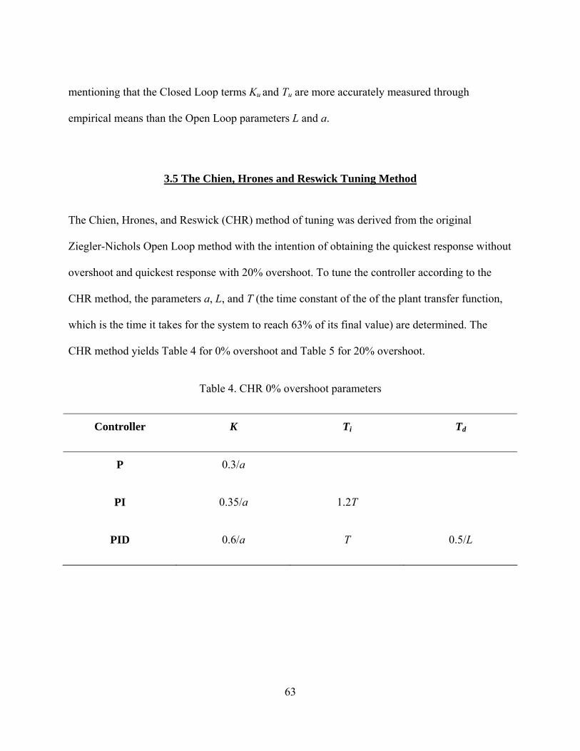
CHR method yields Table 4 for 0% overshoot and Table 5 for 20% overshoot.

Table 4. CHR 0% overshoot parameters

Controller K Ti Td

P 0.3/a

PI 0.35/a 1.2T

PID 0.6/a T 0.5/L

64

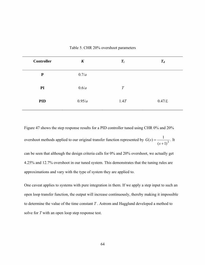
Table 5. CHR 20% overshoot parameters

Controller K Ti Td

P 0.7/a

PI 0.6/a T

PID 0.95/a 1.4T 0.47/L

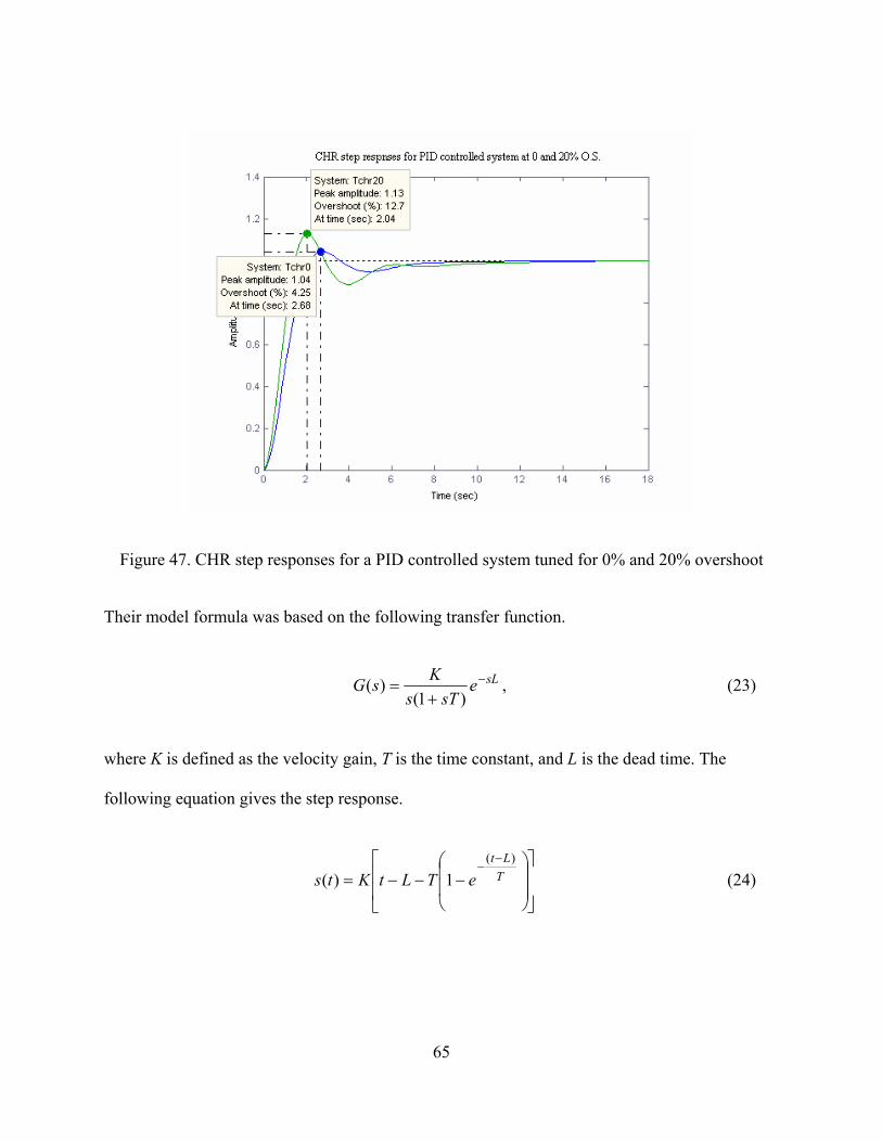
Figure 47 shows the step response results for a PID controller tuned using CHR 0% and 20%

overshoot methods applied to our original transfer function represented by 3)1(1)(+

=s

sG . It

can be seen that although the design criteria calls for 0% and 20% overshoot, we actually get

4.25% and 12.7% overshoot in our tuned system. This demonstrates that the tuning rules are

approximations and vary with the type of system they are applied to.

One caveat applies to systems with pure integration in them. If we apply a step input to such an

open loop transfer function, the output will increase continuously, thereby making it impossible

to determine the value of the time constant T . Astrom and Hagglund developed a method to

solve for T with an open loop step response test.

65

Figure 47. CHR step responses for a PID controlled system tuned for 0% and 20% overshoot

Their model formula was based on the following transfer function.

sLesTs

KsG −

+=

)1()( , (23)

where K is defined as the velocity gain, T is the time constant, and L is the dead time. The

following equation gives the step response.

⎥⎥

⎦

⎤

⎢⎢

⎣

⎡

⎟⎟

⎠

⎞

⎜⎜

⎝

⎛−−−=

−−

TLt

eTLtKts)(

1)( (24)

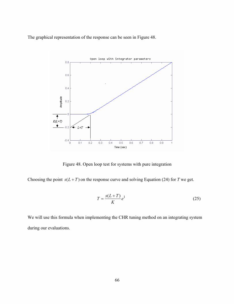
66

The graphical representation of the response can be seen in Figure 48.

Figure 48. Open loop test for systems with pure integration

Choosing the point )( TLs + on the response curve and solving Equation (24) for T we get.

1)( eK

TLsT += (25)

We will use this formula when implementing the CHR tuning method on an integrating system

during our evaluations.

67

3.6 The Rule of Thumb Method

Having worked in industry for the past twenty years both as a technician and a systems engineer,

this author has been in many conversations involving the correct method to tune a PID loop. One

such method worth mentioning will be referred to as the Rule of Thumb method. The reason for

this reference is that we cannot find any real definition of the tuning rule or any example of the

math behind it. The rule has simply been passed on by word of mouth. When asking several

engineers how to tune a loop, many of them reply with this or a very similar rule of thumb

method. To reiterate, the motivation behind this thesis is to consolidate and validate the most

common tuning rules used in industry.

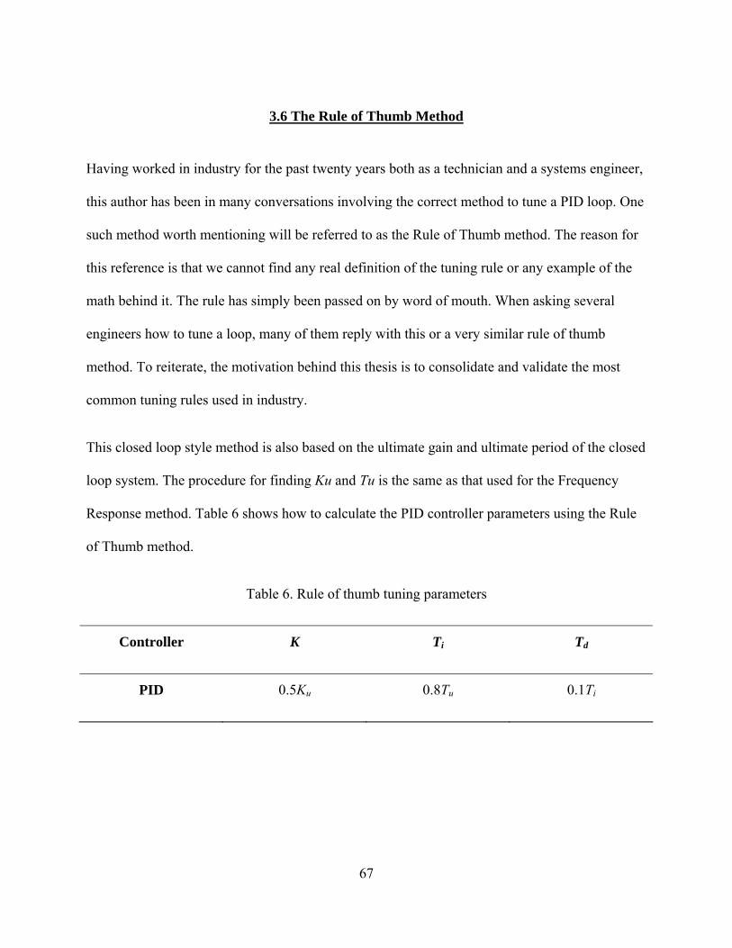
This closed loop style method is also based on the ultimate gain and ultimate period of the closed

loop system. The procedure for finding Ku and Tu is the same as that used for the Frequency

Response method. Table 6 shows how to calculate the PID controller parameters using the Rule

of Thumb method.

Table 6. Rule of thumb tuning parameters

Controller K Ti Td

PID 0.5Ku 0.8Tu 0.1Ti

68

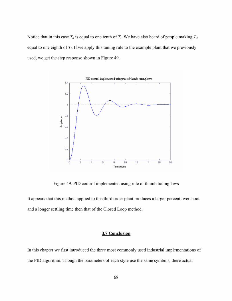
Notice that in this case Td is equal to one tenth of Ti. We have also heard of people making Td

equal to one eighth of Ti. If we apply this tuning rule to the example plant that we previously

used, we get the step response shown in Figure 49.

Figure 49. PID control implemented using rule of thumb tuning laws

It appears that this method applied to this third order plant produces a larger percent overshoot

and a longer settling time then that of the Closed Loop method.

3.7 Conclusion

In this chapter we first introduced the three most commonly used industrial implementations of

the PID algorithm. Though the parameters of each style use the same symbols, there actual

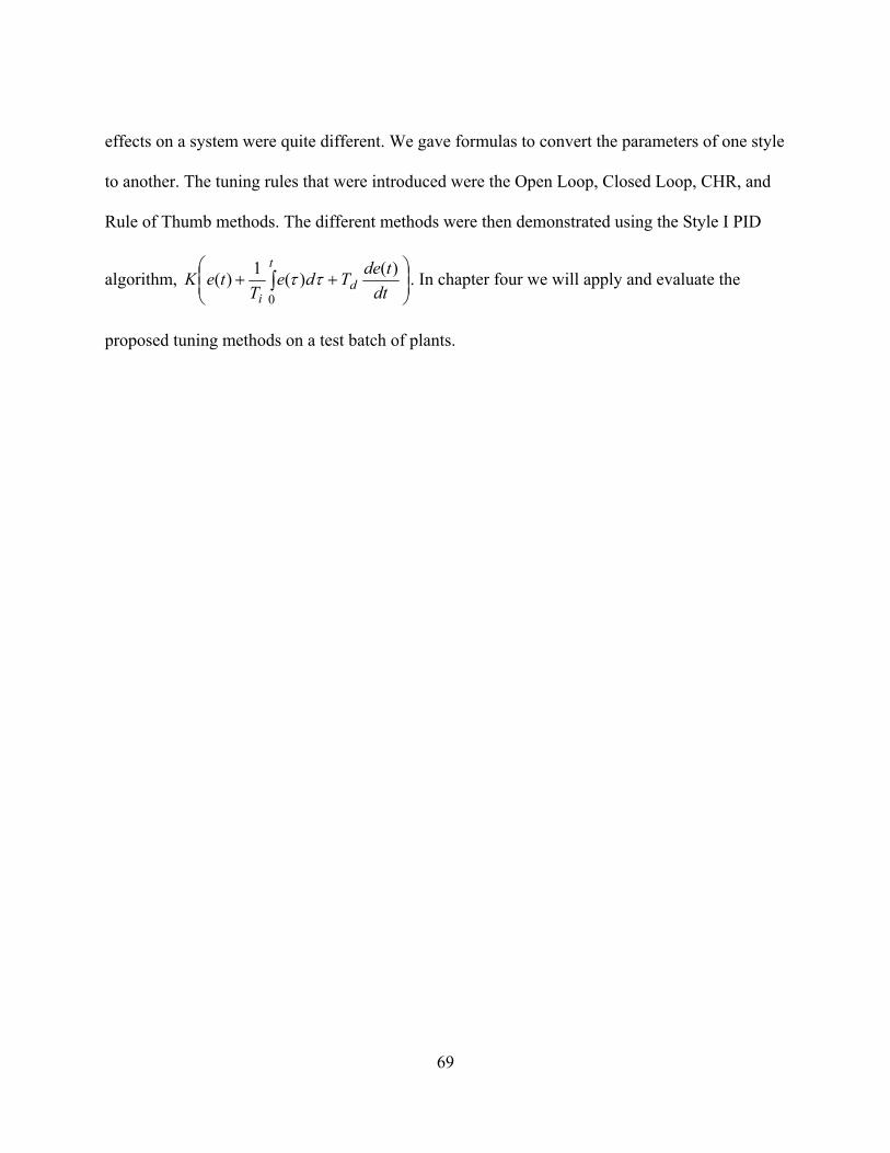
69

effects on a system were quite different. We gave formulas to convert the parameters of one style

to another. The tuning rules that were introduced were the Open Loop, Closed Loop, CHR, and

Rule of Thumb methods. The different methods were then demonstrated using the Style I PID

algorithm, ⎟⎟⎠

⎞⎜⎜⎝

⎛++ ∫

t

di dt

tdeTdeT

teK0

)()(1)( ττ . In chapter four we will apply and evaluate the

proposed tuning methods on a test batch of plants.

70

CHAPTER 4: SIMULATION OF THE STANDARD TUNING METHODS

4.1 Introduction

In this chapter we will apply the proposed tuning methods to a set of test case plants. The plants

modeled will be typical stable systems that can be found in the manufacturing and process

industries. The methods to be tested will be the Open Loop, Closed Loop, CHR, and Rule of

Thumb. The CHR method will only be evaluated for the 0% overshoot implementation. This is

because the 20% implementation closely resembles the Open Loop method which strived for

25% decay ratio. We will evaluate each system by applying a step input to it and comparing

percent overshoot and settling time. In chapter five we will examine the results and draw our

conclusions.

4.2 The Test Batch

The chosen systems for our plant transfer functions will be stable, commonly seen systems in

industry. The first system will be a second order lag with an integrator in the form of:

21)1(

1)(+

=Tss

sG T = 0.1, 1 (26)

The next test case will be a higher order system in the form of:

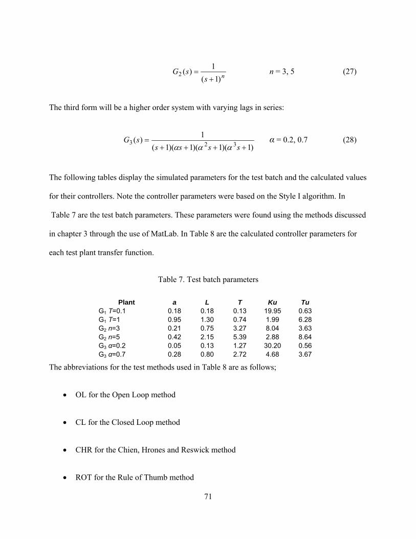
71

nssG

)1(1)(2+

= n = 3, 5 (27)

The third form will be a higher order system with varying lags in series:

)1)(1)(1)(1(1)( 323

++++=

sssssG

ααα α = 0.2, 0.7 (28)

The following tables display the simulated parameters for the test batch and the calculated values

for their controllers. Note the controller parameters were based on the Style I algorithm. In

Table 7 are the test batch parameters. These parameters were found using the methods discussed

in chapter 3 through the use of MatLab. In Table 8 are the calculated controller parameters for

each test plant transfer function.

Table 7. Test batch parameters

Plant a L T Ku Tu G1 T=0.1 0.18 0.18 0.13 19.95 0.63 G1 T=1 0.95 1.30 0.74 1.99 6.28 G2 n=3 0.21 0.75 3.27 8.04 3.63 G2 n=5 0.42 2.15 5.39 2.88 8.64 G3 α=0.2 0.05 0.13 1.27 30.20 0.56 G3 α=0.7 0.28 0.80 2.72 4.68 3.67

The abbreviations for the test methods used in Table 8 are as follows;

• OL for the Open Loop method

• CL for the Closed Loop method

• CHR for the Chien, Hrones and Reswick method

• ROT for the Rule of Thumb method

72

Table 8. Calculated controller parameters

Plant /Method K Ti Td G1 T=0.1 / OL 6.67 0.36 0.09G1 T=1 / OL 1.26 2.60 0.65G2 n=3 / OL 5.71 1.50 0.38G2 n=5 / OL 2.86 4.30 1.08G3 α=0.2 / OL 24.00 0.26 0.07G3 α=0.7 / OL 4.29 1.60 0.40G1 T=0.1 / CL 11.97 0.31 0.079G1 T=1 / CL 1.19 3.14 0.79G2 n=3 / CL 4.82 1.82 0.45G2 n=5 / CL 1.73 4.32 1.08G3 α=0.2 / CL 18.12 0.28 0.07G3 α=0.7 / CL 2.81 1.84 0.46G1 T=0.1 / CHR 3.33 0.13 0.09G1 T=1 / CHR 0.63 0.74 0.65G2 n=3 / CHR 2.86 3.27 0.38G2 n=5 / CHR 1.43 5.39 1.08G3 α=0.2 / CHR 12.00 1.27 0.07G3 α=0.7 / CHR 2.14 2.72 0.40G1 T=0.1 / ROT 9.98 0.50 0.05G1 T=1 / ROT 0.99 5.03 0.50G2 n=3 / ROT 4.01 2.91 0.29G2 n=5 / ROT 1.44 6.91 0.69G3 α=0.2 / ROT 15.10 0.45 0.05G3 α=0.7 / ROT 2.34 2.94 0.29

4.3 The Tests

In this section we will plot all of our PID controlled system step responses. The plots will be

broken up as follows. Each open loop style method of tuning will be on the same plot; likewise

for each closed loop style of tuning. We will further divide the plots by plant transfer function

type being controlled and there two test cases.

73

Figure 50. Plant G1 T=0.1 OL and CHR methods

Figure 51. G1 T=1 OL and CHR methods

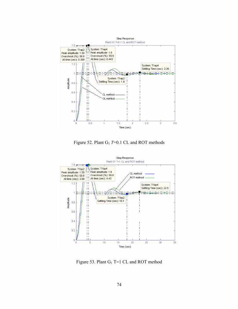
74

Figure 52. Plant G1 T=0.1 CL and ROT methods

Figure 53. Plant G1 T=1 CL and ROT method

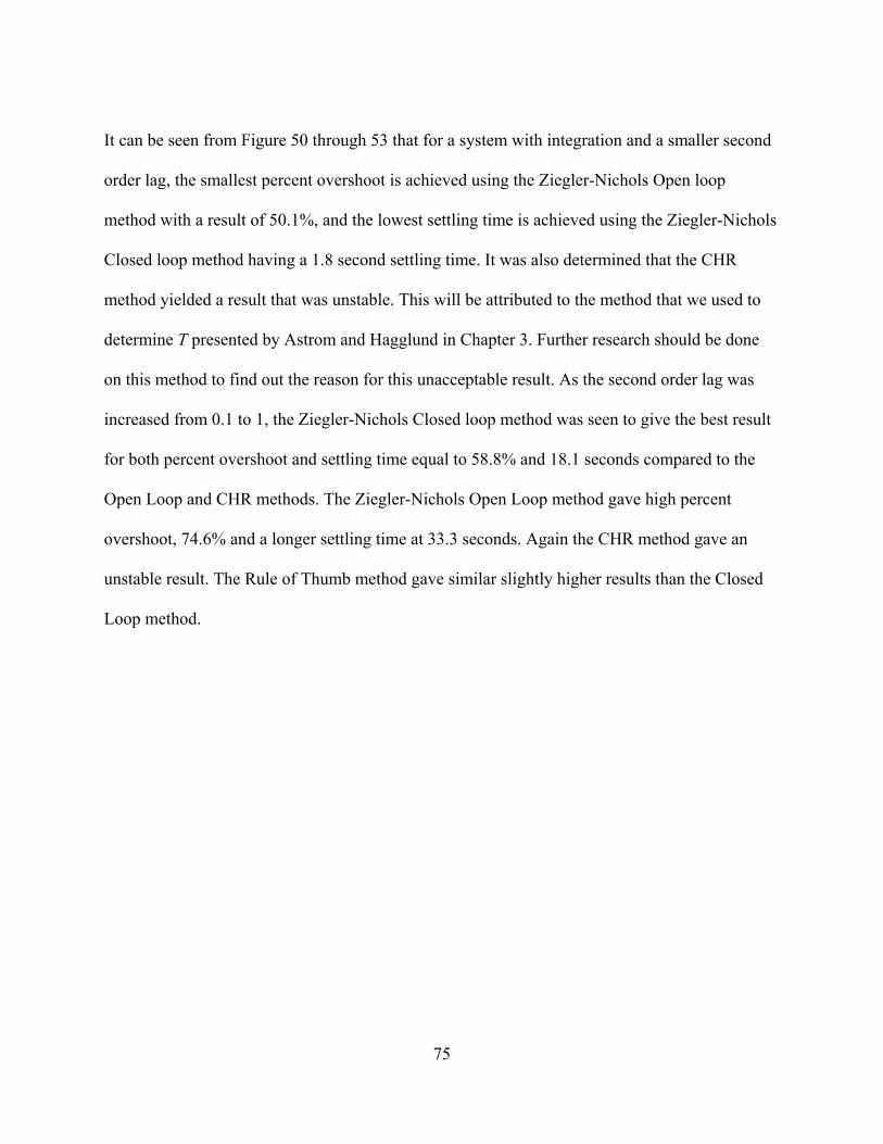
75

It can be seen from Figure 50 through 53 that for a system with integration and a smaller second

order lag, the smallest percent overshoot is achieved using the Ziegler-Nichols Open loop

method with a result of 50.1%, and the lowest settling time is achieved using the Ziegler-Nichols

Closed loop method having a 1.8 second settling time. It was also determined that the CHR

method yielded a result that was unstable. This will be attributed to the method that we used to

determine T presented by Astrom and Hagglund in Chapter 3. Further research should be done

on this method to find out the reason for this unacceptable result. As the second order lag was

increased from 0.1 to 1, the Ziegler-Nichols Closed loop method was seen to give the best result

for both percent overshoot and settling time equal to 58.8% and 18.1 seconds compared to the

Open Loop and CHR methods. The Ziegler-Nichols Open Loop method gave high percent

overshoot, 74.6% and a longer settling time at 33.3 seconds. Again the CHR method gave an

unstable result. The Rule of Thumb method gave similar slightly higher results than the Closed

Loop method.

76

Figure 54. Plant G2 n=3 OL and CHR method

Figure 55. Plant G2 n=3 CL and ROT methods

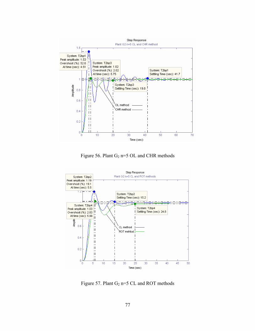
77

Figure 56. Plant G2 n=5 OL and CHR methods

Figure 57. Plant G2 n=5 CL and ROT methods

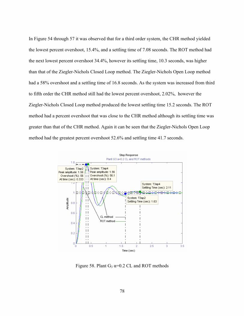
78

In Figure 54 through 57 it was observed that for a third order system, the CHR method yielded

the lowest percent overshoot, 15.4%, and a settling time of 7.08 seconds. The ROT method had

the next lowest percent overshoot 34.4%, however its settling time, 10.3 seconds, was higher

than that of the Ziegler-Nichols Closed Loop method. The Ziegler-Nichols Open Loop method

had a 58% overshoot and a settling time of 16.8 seconds. As the system was increased from third

to fifth order the CHR method still had the lowest percent overshoot, 2.02%, however the

Ziegler-Nichols Closed Loop method produced the lowest settling time 15.2 seconds. The ROT

method had a percent overshoot that was close to the CHR method although its settling time was

greater than that of the CHR method. Again it can be seen that the Ziegler-Nichols Open Loop

method had the greatest percent overshoot 52.6% and settling time 41.7 seconds.

Figure 58. Plant G3 α=0.2 CL and ROT methods

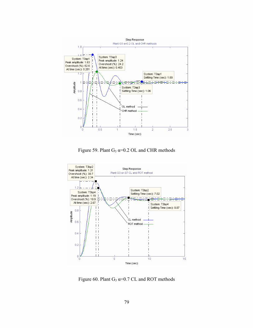
79

Figure 59. Plant G3 α=0.2 OL and CHR methods

Figure 60. Plant G3 α=0.7 CL and ROT methods

80

Figure 61. Plant G3 α=0.7 OL and CHR methods

For systems with varying lags in series based on α=0.2, we see that the CHR method achieved

the lowest percent overshoot 24.2% as well as settling time at 1.06 seconds. All other methods

produced results of percent overshoot within the 55 to 65 percent range, however their settling

times were not too much greater than that of the CHR method. When we increased to α=0.7,

again the CHR method yielded the smallest percent overshoot at 11% and the lowest settling

time of 6.24 seconds. The ROT method gave the next lowest percent overshoot at 18.9% while

the Ziegler-Nichols Closed Loop method had the next lowest settling time of 7.02 seconds. The

Ziegler-Nichols Open Loop method resulted in the highest percent overshoot and settling time.

81

In Table 9 we have tabulated the results from our twenty four tests that were ran.

Table 9. PID controlled systems step response results

Plant Tuning Method % OS

Settling Time

(seconds) G1(s) T=0.1 OL 50.1 2.19 G1(s) T=0.1 CHR NA NA G1(s) T=0.1 CL 58.8 1.8 G1(s) T=0.1 ROT 59.9 2.26

G1(s) T=1 OL 74.6 33.3 G1(s) T=1 CHR NA NA G1(s) T=1 CL 58.8 18.1 G1(s) T=1 ROT 59.8 22.5 G2(s) n=3 OL 58 16.8 G2(s) n=3 CHR 15.4 7.08 G2(s) n=3 CL 40.5 9.35 G2(s) n=3 ROT 34.4 10.3 G2(s) n=5 OL 52.6 41.7 G2(s) n=5 CHR 2.02 19.8 G2(s) n=5 CL 19.1 15.2 G2(s) n=5 ROT 2.83 24.8

G3(s) α=0.2 OL 62.6 1.69 G3(s) α=0.2 CHR 24.2 1.06 G3(s) α=0.2 CL 56 1.63 G3(s) α=0.2 ROT 56.1 2.11 G3(s) α=0.7 OL 59 14.5 G3(s) α=0.7 CHR 11 6.24 G3(s) α=0.7 CL 30.7 7.02 G3(s) α=0.7 ROT 18.9 9.87

82

CHAPTER 5: CONCLUSIONS AND ALTERNATIVES

5.1 Conclusions

In this thesis we have presented and evaluated four different methods used in industry to tune

PID controllers. The motivation behind this was the fact that when surveying several engineers

and technicians regarding what is the best way to tune a PID loop for a plant whose transfer

function was unknown, we would usually get several different answers. The four methods were

chosen because they are the more popular ones that this engineer has seen; also we wanted to

evaluate open loop methods as well as closed loop methods of tuning.

In chapter two we reviewed the building blocks that make up the PID controller and gave design

examples of each: the P, PI, and PD controller. We then reviewed the root locus design method

for a PID controller. This was done to demonstrate the work that is required to tailor a controller

to a particular process when the plant transfer function is known. All design criteria were based

on % overshoot and settling time.

In chapter three the three most popular implementations of the PID algorithm used in industry

were introduced. We reinforced the fact that the engineer responsible for tuning a control system

must know the exact form of the algorithm used in order to apply the tuning rules set forth, and

must be able to convert parameters from one algorithm to the other, otherwise the results will be

undesirable. As stated in chapter one, the lack of knowledge of the form of the algorithm used

accounts for many of the poorly tuned control systems in industry. We then introduced our four

83

tuning methods to be evaluated. We deliberately chose two open loop style methods and two

closed loop style methods. The Ziegler-Nichols Open Loop method and the CHR method were

chosen for our open loop styles. The Ziegler-Nichols Closed Loop method and the so called Rule

of Thumb method were chosen as our closed loop styles. We then gave examples of how to

apply these methods to a sample plant.

In chapter four we chose three sets of test cases to apply our tuning rules to. These sample plants

were open loop stable linear time invariant models. Our first test case was that of a system with a

pure integration and a second order lag. The next system evaluated was one that had a higher

order than two. The third system evaluated was one of higher order with varying lags in series.

We applied our tuning rules on each system and evaluated their performance based on their

percent overshoot and settling time to a step input. All controllers were of the Style I type and

simulations were performed using MatLab. The twenty four test results were tabulated in

Table 8.

After careful scrutiny of our test results the following conclusions were made. No one single

method consistently gave the lowest percent overshoot and settling time for each type of plant.

Depending on the desired operating criteria, further manual fine tuning will probably be needed

for all tuning methods. For systems with pure integration in them, the Open Loop method of

tuning yielded the best results in percent overshoot, however the Closed Loop method had the

shortest settling time. As the lag time increased in the integrated system, the Closed Loop

method had the best all around results. The CHR method applied to a system with pure

integration in it did not fair well at all. It can be seen from Figures 50 and 51 that the CHR

method yielded unstable systems. This may be due to the method we used to calculate the system

84

time constant T that we introduced in chapter three. For our higher order systems, the CHR

method gave the best performance, however it was noticed as we increased the order of the

system, the Closed Loop method gave us a shorter settling time yet its percent overshoot was

quite high at 56% as compared to that of the CHR method, whose overshoot was at 24.2%. For

our fourth order system with varying lags in series, the CHR method consistently gave the best

results. The Rule of Thumb method usually gave similar results to that of the Closed Loop

method, however for higher order systems the Rule of Thumb method gave less percent

overshoot but with a longer settling time than the Closed Loop method.

Since these tuning methods are used when the plant transfer function is not known, and none of

them were found to give consistently the lowest percent overshoot and settling time for all plants

tested, there cannot be a recommendation as to which method an engineer should choose to use.

If the plant transfer function is known or can be reasonably modeled then the following

recommendations can be followed, when tuning systems with pure integrations in their transfer

function, the Open Loop or Closed Loop method be used. When tuning systems of order higher

than two, the CHR or Closed Loop method should be used, however for high order systems with

varying lags the CHR method should be used.

5.2 Available Alternatives

After reviewing the tuning method test results there appears to be a need to develop better, i.e.

more predictable tuning rules, for systems where the plant is unknown. There are alternatives

85

available. Adaptive controllers are available in different configurations. Model Reference

Adaptive Controllers (MRACs) which incorporate a reference model, defining desired closed

loop performance. Another style controller is the Model Identification Adaptive Controller

(MIACs) which performs system identification while the system is running.

86

LIST OF REFERENCES

[ACL05] Ang, Chong, Li. PID Control System Analysis, Design, and Technology, IEE

2005.

[MW98] Dr. M.J. Willis, Proportional-Integral-Derivative Control, 1998 Lecture notes.

[SB93] Stuart Bennett, Development of the PID Controller, IEEE Control Systems, 1993.

[DSC05] David W. St. Clair, Controller Tuning and Control Loop Performance, 2005

[ZN42] J.G Ziegler and N.B Nichols, Optimum settings for automatic controllers, 1942

[ZN43] J.G Ziegler and N.B Nichols, Process lags in automatic control circuits, 1943

[NN04] Norman S. Nise, Control Systems Engineering Fourth Edition, 2004

[GE04] George Ellis, Control System Design Guide, 2004

[AH95] K. Astrom and T. Hagglund, PID Controllers: Theory, Design, and Tuning, 1995

[LE00] B. Lurie and P Enright, Classical Feedback Control, 2000

[MR04] M Ruel, Tuning Loops Quickly at Startup, 2004