UNIVERSITA’ DEGLI STUDI DI BERGAMO DIPARTIMENTO DI INGEGNERIA GESTIONALE

QUADERNI DEL DIPARTIMENTO†

Department of Economics and Technology Management

Working Paper

n. 04 – 2009

A comparative study of airport connectivity in China, Europe and US:

which network provides the best service to passengers?

by

Stefano Paleari, Renato Redondi, Paolo Malighetti

† Il Dipartimento ottempera agli obblighi previsti dall’art. 1 del D.L.L. 31.8.1945, n. 660 e successive modificazioni.

COMITATO DI REDAZIONE§ Lucio Cassia, Gianmaria Martini, Stefano Paleari, Andrea Salanti § L’accesso alla Collana dei Quaderni del Dipartimento di Ingegneria Gestionale è approvato dal Comitato di Redazione. I Working Papers della Collana costituiscono un servizio atto a fornire la tempestiva divulgazione dei risultati dell’attività di ricerca, siano essi in forma provvisoria o definitiva.

A comparative study of airport connectivity in China, Europe and

US: which network provides the best service to passengers?

Stefano Paleari*, Renato Redondi**, Paolo Malighetti***

* Department of Economics and Technology Management, University of Bergamo, Scientific

Director of ICCSAI, Viale G.Marconi, 5 - 24044 Dalmine (BG) Italy

** Department of Mechanic Engineering, University on Brescia, Italy

*** Department of Economics and Technology Management, University of Bergamo, Italy;

Tel. +39 035 2052023 - Fax. +39 02 700423094; e-mail paolo.malighetti@unibg.it

Abstract

This paper investigates the connectivity of the airport networks in China, Europe and US. Our

aim is to analyze which network is most beneficial to final passengers in terms of travel time

and which of the network features lead to such a result. A time-dependent minimum path

approach is employed to calculate the minimum travel time between each pair of airports in

the three networks, inclusive of flight times and waiting times in intermediate airports. We

evaluate each fastest indirect connection in terms of circuitry times and routing factors to

consider the effect of the hubs’ locations. Then we assess the temporal coordination of flights

by calculating the average waiting times in intermediate airports. Our results show that fastest

connections do not differ much in terms of routing factors and circuitry times. Even if the

European network has the greater number of direct flights per airport, when connections

require intermediate airports, their average waiting times exceed those of the American and

Chinese Network.

Keywords: 1) Airport connectivity, 2) Network features, 3) travel time

1. Introduction

The air transportation network has an enormous impact on economies, social evolution and

community welfare at the local, national, and international levels. This is confirmed by the attention

paid by policy-makers and the media to problems with its efficiency and safety. It is thus interesting

to investigate and compare different airport networks in terms of the features and connectivity they

offer. Moreover, the ongoing growth and liberalization of air transport systems worldwide have

spurred rapid development of the industry.

While not yet at the point of a “single playfield”, liberalization has already increased the size of

several common aviation areas. Among the biggest are the US domestic market and the European

common aviation area. The Chinese network is also interesting in terms of size and recent growth.

These networks account for 51.1% of all seats offered worldwide (see Table 1). The three networks

are also subject to homogeneous internal aviation laws developed differently. Finally, they all

present complex dynamics similar to the worldwide airport network. The aim of this paper is to

compare the features and connectivity offered by the three major networks, and to discover the

reasons behind any differences.

Airport network % of routes

worldwide

% of flights

worldwide

% of seats offered

worldwide

US domestic 19.0% 28.4% 22.2%

EU domestic + intra EU 22.3% 22.8% 23.9%

Chinese domestic 4.9% 4.4% 5.0%

overall 46.2% 55.6% 51.1%

Table 1. The sizes of three local networks compared to the overall worldwide network. Source: our analysis of the

Innovata database. The data refer to flights scheduled for 24 October 2007.

2. Literature review

In the framework of network analysis, airports represent nodes and individual routes represent

the connections between them. The resulting structure is interesting in terms of both topological

features and what it reveals about network performance from the passenger’s perspective. The first

topic draws from the literature on complex networks, while the second falls under the topic of air

transport economics and evolution.

 3 

An airport network’s topology can be analyzed by employing graph theory. The field of complex

network analysis has developed powerful tools for studying integrated structures and their

dynamics. The main characteristics of a network can be inferred from its N×N adjacency matrix (N

being the number of nodes) whose elements aij are 1 if node i and node j are connected, and 0

otherwise. Another N×N matrix contains the weight of each connection, which in the context of

aviation may well be the distance of the route. Typical measures characterizing a network are the

distribution degree (the typical number of edges starting from a node) and the clustering coefficient

(quantifying the connectivity among immediate neighbors).

Recent advances by Watts and Strogatz (1998), Barabási and Albert (1999), Amaral et al.

(2000), and Albert and Barabási (2002) have boosted the scope of complex network theory. They

defined the concept and features of a “small world network”. Furthermore, Costa and Silva (2006)

found that the distribution degree allows one to define a node hierarchy, leading to a taxonomy of

relationships between the nodes. Guimerà et al. (2007) divided complex networks into two distinct

functional classes on the basis of their connection frequency. The topology of a network is strictly

related to the dynamics of its formation (Watts and Strogatz, 1998; Watts, 1999). For this reason,

growth determinants and future evolution may be inferred from a network’s current topology

(Barrat et al., 2004).

Previous studies have classified airport systems as small world, scale-free networks (Guimerà et

al. 2005; Bagler, 2004; Li and Cai, 2004). This means that new links are more likely to be appended

to nodes with higher connectivity, yielding a power law distribution of airport degrees.

Capacity saturation and political barriers partially distort the actual network topology from the

theoretical one. Guimerà et al. (2005), analyzing the worldwide airport network, found that the most

central cities are not always the most connected for political reasons. Bagler (2004) found that the

Indian airport network is of the small world type, but that the incremental cost of additional

capacity in bigger airports truncates the scale-free power law distribution. Li and Cai (2004)

classified the topology of the Chinese airport network as intermediate between a random graph and

a scale-free network. Analyzing the Italian airport network, Guida and Funaro (2007) detected a

small world, scale-free network with fractal structure.

One of the main features of a network is its mobility (Milgram, 1977), defined as the ease of

traveling from one node to another. Mobility measures are based on the minimum path between any

given pair of nodes. In the simplest case, they may represent the number of steps needed to travel

from one node to another. In more complex cases, each step is weighted by one or more proxies for

 4 

the importance of nodes and edges. In the field of airport networks, connections may be weighted

by frequency of operation, number of seats offered, or geographical distance.

Latora and Marchiori (2001) introduced the related concept of efficiency, which measures how

easily information is exchanged over the network. In the field pf airport networks, Latora and

Marchiori definition of efficiency is represented by the extra distance involved in the shortes path

between any airport pairs compared to the direct distance. An efficiency of 1 is possible only when

each node is connected to every other. Latora and Marchiori (2001) showed that small-world

networks are highly efficient. A similar efficiency measure is employed by Li and Cai (2004) in

their analysis of the Chinese airport network, obtaining a score of 0.484.

Following these definitions, a network is efficient when travel within it is equally easy in any

direction, with no reference to overall costs or unit costs. This property might better be called the

effectiveness or feasibility of a network.

The main drawback of complex network analysis is its failure to take into account the temporal

coordination of airport networks. In many cases, the additional utility derived from connecting to a

high-degree airport is the chance to use this airport as an intermediate step to other destinations. But

an interconnection is really feasible only if incoming and outgoing flights at the intermediate airport

occur within a reasonably narrow window. Veldhius (1997), Burghouwt and de Wit (2005), and

Burghouwt (2007) measured the number of flights that can be interconnected considering a time

windows between arrival and departure ranging from 45 minutes up to 3 hours. Both studies

developed an index of indirect connectivity between hub airports and worldwide destinations. Other

studies (Bagler, 2004, Li and Cai, 2004) have tried to consider temporal coordination by weighting

the airport network by frequency. Both approaches essentially evaluate the number of connections

that a passenger passing through the airport could exploit. However, note that many of these

connections will not lie on the quickest path towards a passenger’s final destination. Malighetti et

al. (2008) overcame this problem by computing minimum paths in terms of the quickest travel time

between any pair of airports as a function of departure hour, including both flight time and waiting

time in intermediate airports. The present paper takes a similar approach to calculating travel times,

but uses this information to compare the effective mobility granted by the Chinese, European and

US networks.

3. Methodology

The goal of this paper is to compare the structure and performance of the three airport networks.

Minimum paths in the networks are calculated in terms of minimum travel time between nodes,

including both flight time and waiting time in intermediate airports, and are assumed to depend on

 5 

the passenger’s departure hour. This methodology, based on the theoretical work of Miller-Hooks

and Patterson (2004), was recently employed in Malighetti et al. (2008) to quantify the effectiveness

of the self-help hubbing strategy in the European network.

In order to guarantee the feasibility of connections and the reliability of travel times, we consider

only scheduled flights operating on a specific and typical day in the autumn schedule: Wednesday,

the 24th of October 2007.

The minimum waiting times at intermediate airports may be influenced by several factors: the

presence of dedicated facilities to manage transfer passengers, the degree of airport congestion, and

the airport’s overall size. In this paper we assume a minimum interconnecting period of 60 minutes

for all intermediate airports. This lower limit does not apply in the case of multi-leg trips

coordinated directly by a carrier or an alliance, for which the passenger has just one ticket to their

final destination. In such cases we take the interconnection waiting period directly from the flight’s

schedule. In some cases the waiting periods for a multi-leg trip can be less than 45 minutes,

especially in small intermediate airports and flights where connecting passengers do not leave the

aircraft.

In other cases a 60-minute minimum interconnecting period is acceptable since we aim to

compare the internal connections of the three major networks; no intercontinental flights are

included in the study. No maximum connecting time is assumed.

As described in Malighetti et al. (2008), the shortest travel time STTijt from airport i to airport j

is calculated starting at a specified time t. The day is divided into 96 units of fifteen minutes, so

starting times range from 00:00 to 23:45. For the European network we work in Brussels time, for

the US network we work in New York time, and for the Chinese network we work in Beijing time.

Itineraries ending after midnight are not taken into account. Thus, for every possible combination of

two airports at a given starting time t, we calculate the shortest travel time for all itineraries leaving

as early as 00:00 and concluding before midnight of the same day. The minimum travel time from

airport i to j is then defined as STTij=mint(STTijt).

After calculating the shortest travel times within each network, we investigate their determinants

to explain possible differences. In particular, we would like to evaluate the impact of the following

three variables: i) connection distance, ii) the relative position of intermediate airports, and iii)

waiting time in intermediate airports.

The first factor is simply defined as the geographical distance between the origin airport and the

final destination airport. The second and third factors are relevant only to connections requiring

more than one flight. Thus, to quantify the effect of an intermediate airport on the route, we

 6 

consider both routing factors (the ratio between indirect and direct flight distances) and circuitry

times (the ratio between total flight time and the flight time supposing to fly directly between the

departure and destination airports).

To evaluate the overall impact of a given airport on waiting times, we need to know how many

quickest paths pass through it, when passengers arrive, and what time the flights to their final

destinations actually depart. In other words, further analysis is required to assess the temporal

coordination of flights at intermediate airports. The first factor is given by the betweenness of each

airport, as described in Freeman (1977) and Malighetti et al. (2008). We define the routing factor as

the ratio between in-flight distance and potential direct flight distance. In this paper, we consider

only itineraries with a routing factor of at most 1.25. This upper limit excludes indirect connections

with excessive detours, even if they are among the shortest possible routes between airports.

As is usual for research focusing on travel times, our work neither assesses traveler utility nor

models the passenger’s choice of route and airports. To do so would entail a much more complex

set of variables, including fares.

4. Data

All our data refer to flights scheduled on 24 October 2007, as published in the Innovata

database’s winter 2007 release. By analyzing a specific day, we consider actual projected

connections rather than an average daily schedule with only theoretical significance. In particular,

the latter would not guarantee the feasibility of all connections. The specific day was chosen to

avoid demand peaks. We include all airports with at least one scheduled flight to another airport of

the network. The European network includes all countries of the EU25 plus Switzerland, Norway

and Iceland. The US network contains 657 airports, the European network 467 airports, and the

Chinese network 143 airports.

Each network is of course connected to the global airport system. Nevertheless, the majority of

routes offered occur entirely within each network. This is particularly true of the US network,

where 82.3% of routes are domestic (Table 2). In the present analysis, we only consider internal

connections.

Figure 1 represents the three networks on the day considered. While the US network has the

most nodes, the European network has the most direct connections. The structures of the networks

are clearly quite different: in Europe the major airports are all close to one other, while in US and

China they are quite dispersed.

 7 

US, EU and CN airport network

Figure 1.The airport networks of the US, the EU and China. The bright blue lines are drawn for 10% of routes in each

network, those offering the greatest number of seats.

 8 

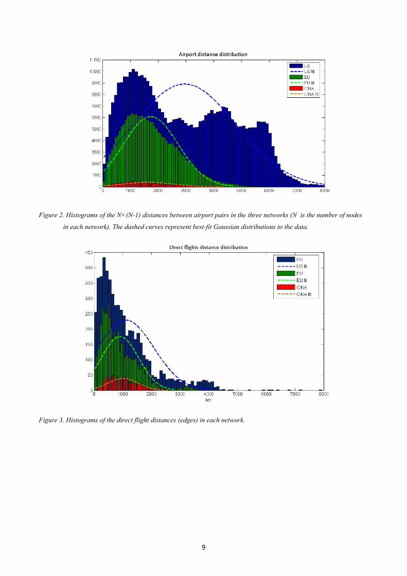
Figure 2 provides histograms of the N×(N−1) distances (N being the number of nodes in each

network) between airport pairs in each network. In Europe, connection distances are concentrated

around 1000-1200 km with a bell-shaped distribution close to Gaussian. In China the relative

dispersion of distances is far greater, but the Gaussian distribution is still a reasonable description of

the data. The US network, in stark contrast, has several peaks. The two strongest lie around 1000-

1200 km and 4500 km, and are mainly related to travel between airports on the same coast and

opposite coasts respectively.

The three networks appear more similar when only direct flights are included in the distribution

(see Figure 3). All three networks have a strong peak at about 600-800 km, and a secondary peak at

greater distances (3000-4000 km). We suggest two possible explanations for this behavior. The first

is simply that local hubs may play the role of bridges between widely separated areas. Second, this

structure supports the theory that distances influence the dynamic evolution of a network. In other

words, a new edge is more likely to be added between close nodes, at least up to a certain threshold.

Airport

network

No. of

airports

(nodes)

Average

distance between

airport pairs

(km)

No. of routes

within networka

Average

frequency of

intra-network

routes

% of intra-

network routes

US 657 2 954 5 488 4.8 82.3%

EU 467 1 736 5 544 3.1 73.4%

CN 144 1 631 1 329 3.3 75.1%aone-way routes

Table 2. Summary statistics on the three local networks.

 9 

Figure 2. Histograms of the N×(N-1) distances between airport pairs in the three networks (N is the number of nodes

in each network). The dashed curves represent best-fit Gaussian distributions to the data.

Figure 3. Histograms of the direct flight distances (edges) in each network.

 

 

 

 

 10 

5. Empirical analysis

5.1 Network topology

Our topological analysis confirms that all three airport systems belong to the class of small world

networks. Their configurations are similar to the scale-free power law, but are better fit by a double

Pareto law (Reed, 2003):

1

2

1 1

2 2

( ) ( )

c

c

P k c k k kP k c k k k

α

α

εε

−

−

⎧ > = + + ≤⎨

> = + + >⎩

where k is the airport’s degree. The European network (see Table 3 and Figure 4) has the highest

values of α1 and α2, meaning its degree distribution decays more rapidly. One possible explanation

for this difference is that Europe experiences more congestion than the other two regions. The

average shortest path length ranges from 2.34 steps in China to 3.38 steps in the US. In all three

cases, the average shortest path length is very close to that of a comparable random network (with

the same number of nodes and edges). Their clustering coefficients (the probability that two airports

connected with a third one is also direct connected each other), however, are all significantly higher

than those of comparable random networks. Despite the emergence of a point-to-point structure and

greater average degree due to the rise of low-cost carriers, the European network still has the lowest

clustering coefficient.

Average SPL Clustering coeff.

Airport

network

Average

degree measured

~( rnd

network) measured

~( rnd

network)

Critical

degree

kc

α1

(k≤kc)

α2

(k>kc)

US 8.5 3.38 2.80 0.45 0.017 77 0.72 -3.99

EU 12.1 2.80 2.45 0.38 0.027 60 0.80 -4.23

Chinese 9.2 2.34 2.14 0.49 0.074 28 0.51 -2.79

Table 3. Network topology statistics. Columns 4 and 6 report the average shortest path length and the clustering

coefficient of a comparable network (same number of edge and nodes) with a random edge distribution.

 11 

Airport degree distributions

y = ‐0,72x + 0,36R² = 0,97

y = ‐3,99x + 14,48R² = 0,96

‐7

‐6

‐5

‐4

‐3

‐2

‐1

0

0 1 2 3 4 5

ln (P>k)

ln (k)

US network

k<kc k>kc

 

y = ‐0,80x + 0,65R² = 0,96

y = ‐4,23x + 14,54R² = 0,97

‐7

‐6

‐5

‐4

‐3

‐2

‐1

0

1

0 1 2 3 4 5ln (P>k)

ln (k)

EU network

k<kc

k>kc

y = ‐0,51x + 0,09R² = 0,98

y = ‐2,79x + 7,71R² = 0,97

‐6

‐5

‐4

‐3

‐2

‐1

0

0 1 2 3 4 5

ln (P

>k)

ln (k)

CN network

K<Kc

k>kc

‐6

‐5

‐4

‐3

‐2

‐1

0

0 1 2 3 4 5

ln (P

>k)

ln (k)

US‐EU‐CN

CN K<Kc CN k>kc

EU K<Kc EU k>kc

Us k<kc US k>kc

Figure 4. Degree distributions of the three networks. In all three cases the ‘knee’ of the Pareto double power law

distribution is clearly visible in the data. The fourth panel (lower right) superposes the three distributions.

5.2 Travel time analysis

As mentioned at the end of Section 2, any analysis of network topology will fail to take into

account the temporal coordination of flights. We now consider the average time required to go from

a given node to any other node in the network. We also evaluate the average number of steps

required to complete the connections, the quickest connecting path as a function of departure time,

and the routing factors and waiting times associated with the intermediate airports (see Section 3 for

a definition of these quantities).

Departure times for the flights considered range from 6.00 to 23:45. Where available, direct

connections are clearly the shortest travel time option. The case of indirect connections is more

complicated: earlier departures increase the chance of making a connection, but also tend to

increase waiting times. For each airport, we begin by finding the departure time that minimizes the

average travel time to all destinations reachable by midnight of the same day. For airport i this

quantity is the t which minimizes Σj STTijt/N.

 12 

For the majority of the airports in the three networks, as shown in Figure 5, the best departure

time is between 10:30 AM and 12:00 A.M. In the next part of the analysis we consider for each

airport pairs the best shortest travel time available during the day.

Optimal departure times

0

5

10

15

20

25

30

35

40

6.00

6.45

7.30

8.15

9.00

9.45

10.30

11.15

12.00

12.45

13.30

14.15

15.00

15.45

16.30

17.15

18.00

h

US

0

5

10

15

20

25

30

35

6.00

6.45

7.30

8.15

9.00

9.45

10.30

11.15

12.00

12.45

13.30

14.15

15.00

15.45

16.30

17.15

18.00

h

EU

0

2

4

6

8

10

12

6.00

6.45

7.30

8.15

9.00

9.45

10.30

11.15

12.00

12.45

13.30

14.15

15.00

15.45

16.30

17.15

18.00

h

CN

0

5

10

15

20

25

30

35

40

6.00

6.45

7.30

8.15

9.00

9.45

10.30

11.15

12.00

12.45

13.30

14.15

15.00

15.45

16.30

17.15

18.00

h

US

EU

CN

Figure 5. Distributions of optimal departure times (minimizing the average shortest travel time from each airport in the

network to all other airports).

If N is the number of airports in the network, there are N×(N−1) possible one-way connections

between airports. We find that 39.1% of the N×(N−1) theoretical connections in Europe can be

successfully completed by midnight, compared to 28.2% in the US and 29.3% in China. We call

this index “network openness”. This measure is influenced by the upper limit of 1.25 we placed on

routing factors. Even without a routing factor limit, however, in all three networks fewer than half

of theoretical connections can be completed within the analyzed day. The European network has the

highest “openness” both with and without a routing factor limit, due to its large number of short

direct routes. Despite having a higher average frequency overall, longer distances penalize the US

network in terms of “openness”.

 13 

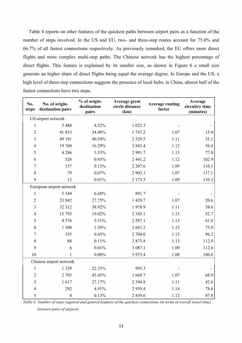
Table 4 reports on other features of the quickest paths between airport pairs as a function of the

number of steps involved. In the US and EU, two- and three-step routes account for 75.0% and

66.7% of all fastest connections respectively. As previously remarked, the EU offers more direct

flights and more complex multi-step paths. The Chinese network has the highest percentage of

direct flights. This feature is explained by its smaller size, as shown in Figure 6 a small size

generate an higher share of direct flights being equal the average degree. In Europe and the US, a

high level of three-step connections suggests the presence of local hubs; in China, almost half of the

fastest connections have two steps.

No. steps

No. of origin-destination pairs

% of origin-destination

pairs

Average great circle distance

(km)

Average routing factor

Average circuitry time

(minutes) US airport network

1 5 488 4.52% 1 022.3 - - 2 41 833 34.48% 1 747.2 1.07 15.43 49 191 40.54% 2 529.5 1.11 35.14 19 760 16.29% 2 843.4 1.12 56.45 4 286 3.53% 2 991.7 1.13 77.06 526 0.43% 2 441.2 1.12 102.97 157 0.13% 2 207.6 1.09 110.18 79 0.07% 2 903.3 1.07 117.19 12 0.01% 2 173.3 1.09 139.3

European airport network 1 5 544 6.68% 891.7 - - 2 23 042 27.75% 1 429.7 1.07 20.63 32 312 38.92% 1 978.9 1.11 38.64 15 795 19.02% 2 345.1 1.13 52.75 4 576 5.51% 2 597.1 1.13 61.86 1 308 1.58% 2 661.2 1.13 75.07 355 0.43% 2 704.0 1.13 96.28 88 0.11% 2 873.8 1.13 112.99 6 0.01% 3 087.1 1.09 112.6

10 1 0.00% 3 973.4 1.08 106.6 Chinese airport network

1 1 329 22.33% 995.3 - - 2 2 705 45.45% 1 668.7 1.07 68.93 1 617 27.17% 2 394.8 1.11 42.64 292 4.91% 2 939.4 1.14 78.65 8 0.13% 2 839.6 1.12 87.8

Table 4. Number of steps required and general features of the quickest connections (in terms of overall travel time),

between pairs of airports.

 14 

0,0%1,0%2,0%3,0%4,0%5,0%6,0%7,0%8,0%9,0%

10,0%

130

170

210

250

290

330

370

410

450

490

530

570

610

650

690

730

770

810

850

n. of airports

Average degree and % of direct connection on overall  possible nodes pair   

8

9

10

11

12

13

average degreeChinesenetwork

European networkUS network

Figure 6. Share of the theoretical direct connections on overall origin-destination pairs as a function of the size of the

network (N) and the average nodes degree (k).

Two-step and three-step paths are necessary for connecting distant airports. Indeed, average

great circle distances is about 800-1,000 km for 1step connection compared to 1.500-2.500 km in

the cases of, two-step and three-step paths. Paths with more than four steps tend to have only a

further slightly increases of the average great circle distance between origin and destination. These

routes often connect minor airports that are not necessarily distant, but part of different and poorly

interconnected sub-networks. We do not find paths longer than five steps in the Chinese network.

Surprisingly, even though the three networks have very different topological features, their

average routing factors fall within a fairly narrow range (from 1.07 to 1.14) with very similar

routing factor values also when compared by number of required steps. This similarity of routing

factors is quite interesting, and suggests that connections with routing factor much higher than 1.1

will almost always have a better alternative. Table 4 thus provides some interesting insights into

hub location and the performance of indirect connection even if it does not consider the effects of

waiting times in intermediate airports.

Now let us introduce also these effects. Table 5 shows the average shortesttravel times for

optimal routes with a given number of steps, including waiting times in intermediate airports. The

average speed is defined as the total optimal travel time divided by the great circle distance. Thus, it

represents the speed going straight to destination “as the crow flies” and requiring the same travel

time. The shorter average distance of direct flights within Europe results in a lower average speed,

 15 

which can be mainly attributed to the lower percentage of time spent at cruise velocity. For direct

flights, we find an average speed close to 500-600 km/h.

For two-step paths the average speed falls to 270-300 km/h due to circuitry times and waiting

times in intermediate airports. Europe is the least efficient network with respect to waiting times; it

averages two hours per connection, accounting for roughly 40% of total travel time. In US, where

airlines widely exploit the “hub & spoke” strategy on domestic routes, waiting times for two-step

connections are on average shorter by 20 minutes. The Chinese network registers an average

waiting time similar to that of the US network.

For three-step paths, waiting times increase by another 2 hours. More precisely, the average

waiting time increases by 114 minutes in the US, 119 minutes in Europe, and 140 minutes in China.

The ratio of flight time to total travel time drops to 53.5% in Europe, 55% in China, and 60% in the

US. In terms of equivalent average speeds, the airline transportation systems become comparable to

high-speed trains. When considering longer paths, in all three networks the ratio of flight time to

travel time levels off at about 50% and the average speed levels off at 200 km/h.

 16 

No. steps

No. of O-D pairs

Average travel time (min) % Flight time Waiting time

(min)

Average “as a crow flies”

speed (km/h)

US airport network 1 5 488 118 100.0% - 521.52 41 833 319 67.9% 102 328.93 49 191 542 60.1% 216 279.94 19 760 683 56.1% 299 249.85 4 286 772 54.6% 350 232.66 526 748 51.3% 363 195.97 157 710 51.3% 346 186.58 79 800 56.4% 348 217.89 12 696 56.0% 306 187.4

European airport network 1 5 544 107.4 100.0% - 498.32 23 042 314 61.3% 121 272.83 32 312 517 53.5% 240 229.44 15 795 669 50.1% 334 210.35 4 576 766 48.9% 391 203.46 1 308 824 48.0% 428 193.87 355 888 47.5% 466 182.78 88 943 48.6% 484 182.79 6 994 48.7% 509 186.3

10 1 1 245 47.0% 660 191.5 Chinese airport network

1 1 329 97 100.0% - 618.82 2 705 353 70.2% 105 283.83 1 617 544 55.0% 245 264.14 292 762 51.7% 368 231.65 8 761 51.5% 369 224.0

Table 5. Average quickest travel times, waiting times at intermediate airports, and speeds of optimal routes connecting

airport pairs in the networks by the given number of steps.

For all departure-destination airport pairs, Figure 7 plots “as the crow flies” speed against the great

circle distance. The number of steps is indicated by color, with direct flights in dark blue.

Equivalent speeds are highest for direct, long-distance flights, which approach 800 km/h in all three

networks. This is a typical cruise speed for short- and medium-haul aircrafts. The more steps in the

route, however, the lower the equivalent speed. Note that among routes with more than four steps,

the relationship between distance and speed becomes linear. All three networks have very similar

features. The Chinese network shows a sparser distribution due to its much lower number of airport

pairs.

 17 

                                                                                      US network 

  

                                    EU network                                                                         CN network 

Figure 7. The relationship between the equivalent “as the crow flies” speed and great circle distance as a function of

the number of steps, plotted separately for all three networks. The dark blue dots represent direct (one-step)

paths. Progressively lighter shades represent more steps.

In order to account for the size of the airports connected by each O-D links, we also calculate a

weighted average of quickest connection waiting times. For direct flights, the waiting time is zero.

The weighting factor for all routes, including direct flights, is the total size (annual seats offered) of

the departure and destination airports.

 18 

The results of this analysis (see Table 6) show shorter waiting times at all levels, since connections

to major airports are generally better projected and coordinated.

For example, two-step paths in Europe require an average waiting time of 121 minutes, but the

weighted average is only 94 minutes. The US network is most efficient at managing two-step

connections, with an weighted average waiting time of only 72 minutes.

Moreover, the role of long-path connections is far less important, meaning that long paths tend to be

necessary only between very small airports.

On average, connections with long waiting times are between small airports. In this case, Europe

shows the highest weighted waiting time, 48.5 minutes,

US EU CN

No. steps Weighted waiting time

contribution to overall average

Weighted waiting time

contribution to overall average

Weighted waiting

time

contribution to overall average

1 0 60.9% 0 57.32% 0 79.3%2 76 36.0% 94 35.79% 92 18.1%3 165 2.8% 202 5.86% 217 2.4%4 251 0.2% 293 0.83% 320 0.2%

>4 320 0.0% 359 0.20% 397 0.0%Average weighted waiting time

32.8 48.5 22.5

Table 6. Weighted average of quickest path waiting times (in minutes) for each network. The weighting factor is the

total size of the origin and destination airports.

5.3 Travel time and secondary airports

In the last part of the empirical analysis, we compare the relative accessibility of primary and

secondary airports in the three networks. Figure 8 reports the probability of reaching a given

fraction of the network by departing from any airport with fewer than k direct connections. The total

rise in this cumulative distribution reflects the role played by small and large airports in the

network. The greatest difference is found in the Chinese network, where on average the probability

of reaching a given portion of the network increases by about 15% passing from small airports to

bigger airports. The US network is much more homogeneous, but the probability of reaching a

given fraction of the network is on average lower than in the EU or China.

 19 

In Europe as in the US, the accessibility of the network doesn’t change much with airport size. On

the other hand, there are great differences in the absolute level of accessibility within Europe. The

probability of reaching 70% of the network is about 50% for airports with less than 30 direct

connections, but his figure drops to less than 10% if one desires to reach 90% of the network.

For example, Considering airport with less than 15 direct connection 1/5 airports reach 90% of the

network as a whole in US , 1/10 in CN and 1/16 in EU; opposite in CN and in EU 7/10 airports

reach at least 30% of the network while in US less than 6/10.

Airport degree and network accessibility

0,0%

10,0%

20,0%

30,0%

40,0%

50,0%

60,0%

70,0%

80,0%

90,0%

5 10 15 20 25 30 35 40 45 50 55 60 65 70 75 80 85 90 95 100

freq

uency  of reaching  x% of the

 weigh

ted 

netw

ork

airport degree <k

US

30%

40%

50%

60%

70%

80%

90%

% network reached

0,0%

10,0%

20,0%

30,0%

40,0%

50,0%

60,0%

70,0%

80,0%

90,0%

5 10 15 20 25 30 35 40 45 50 55 60 65 70 75 80 85 90 95 100

freq

uency  of reaching  x% of the

 weigh

ted 

netw

ork

airport degree <k

EU

30%

40%

50%

60%

70%

80%

90%

% network reached

0,0%

10,0%

20,0%

30,0%

40,0%

50,0%

60,0%

70,0%

80,0%

90,0%

5 10 15 20 25 30 35 40 45 50 55 60 65 70 75

freq

uency  of reaching  x% of the

 weigh

ted ne

twork

airport degree <k

CN

30%

40%

50%

60%

70%

80%

90%

% network reached

40,0%

45,0%

50,0%

55,0%

60,0%

65,0%

5 10 15 20 25 30 35 40 45 50 55 60 65 70 75 80 85 90 95 100

average  weigh

ted ne

twork reacha

ble

airport degree <k

US‐EU‐CN

CN

EU

US

Figure 8. Airport degree and network accessibility.

 20 

Table 7 specifies the number of airports reachable in one day and average waiting times as a

function of origin-destination airport sizes. The airports in the network are divided into four

quartiles based on the number of direct connections, with Group 4 airports having the most. Thus, a

passenger starting from one the biggest airports can reach the vast majority (over 90%) of airports

classified in the same quartile. This figure reaches 96% for the US network. On the other hand, for a

passenger departing from a small airport (Group 1) in the US, the probability of reaching any final

destination of the same dimension by midnight of the same day is less than 5%. The European and

Chinese networks perform significantly better for small airports by this measure. The probability of

reaching a Group 4 airport starting from a Group 1 airport is 51% in the EU, and 34% in China. It

appears that most small airports in the US are located in very remote areas or are very poorly

connected to the rest of the network.

Dividing routes in the same manner, we see that connections between the largest airports result in

the shortest waiting times. When both origin and destination airports belong to Group 4, average

waiting times are less than 40 minutes in all three networks. This low value is not surprising, since

most of the connections between major airports are served by direct flights. The EU network has

higher waiting times than the US network overall. One can relate this finding to the higher

percentage of airports reached in one day; there is a trade-off between the “openness” of the

network and the average waiting time spent in intermediate airports.

 21 

Percentage of airports reachable in one day Average waiting times

US

O/D Group 1 Group 2 Group 3 Group 4 O/D Group 1 Group 2 Group 3 Group 4

Group 1 5%  1%  3%  4% Group 1 162 336 247 357

Group 2 2%  19%  36%  53% Group 2 176 323 271 181

Group 3 3%  36%  62%  79% Group 3 301 263 209 126

Group 4 4%  57%  84%  96% Group 4 208 139 97 32

EU

O/D Group 1 Group 2 Group 3 Group 4 O/D Group 1 Group 2 Group 3 Group 4

Group 1 12%  19%  30%  51% Group 1 393 339  279 205

Group 2 17%  27%  39%  58% Group 2 396 332  280 190

Group 3 25%  38%  50%  71% Group 3 379 283  219 114

Group 4 44%  58%  71%  91% Group 4 237 166  113 38

CN

O/D Group 1 Group 2 Group 3 Group 4 O/D Group 1 Group 2 Group 3 Group 4

Group 1 4%  6%  17%  34% Group 1 326 360  352 243

Group 2 6%  10%  20%  45% Group 2 335 357  295 173

Group 3 16%  19%  46%  77% Group 3 250 257  215 79

Group 4 36%  48%  76%  93% Group 4 127 103  86 13

Table 7. Percentage of airports reachable in one day and average waiting times in intermediate airports. Airports are

grouped into quartiles based on the number of connections, where Group 4 contains the most connected

airports. Each origin-destination (O/D) pair is classified according to the categories of its airports, as shown

on the rows and the columns of the table, before the average is calculated. In the average, O-D pairs are

weighted by the total size of the connected airports.

6. Conclusion

Our study compares the airport networks of the US, Europe and China in terms of accessibility

and shortest travel times (including waiting time at intermediate airports). A topological analysis

confirms that all three networks belong to the small world class, with similar degree distributions

 22 

and clustering coefficients. In order to account for travel times and scheduling coordination, we

calculate departure time-dependent minimum paths between each airport pair in a network. We also

evaluate the quality of indirect connections in terms of circuitry times and routing factors. Our

results show that the three networks do not differ much in terms of routing factors and circuitry

times. About a third of the possible connections may be successfully concluded within a single day,

following a quickest path whose routing factor does not exceed 1.25. The European network

reaches the highest percentage of destinations, at 39.1%.

We assess the temporal coordination of flights by calculating waiting times in intermediate

airports. The analysis shows that waiting times for indirect connections account for between 30%

and 50% of the overall travel times. Even though the European network has the greater number of

direct flights per airport, connections requiring intermediate airports require average waiting times

exceeding those of the American and Chinese networks.

Our analysis does not support a preference for one network over the others. Nevertheless, we do

find evidence for a trade-off between the “openness” of the network and the average waiting times

spent at intermediate airports. In Europe, the policies of individual governments might explain the

high percentage of airports accessible within a single day: each country favors connectivity towards

its own local airports. Such policies reduce the efficiency of coordination between countries,

resulting in higher waiting times. In contrast, the US network shows better coordination (having

benefited from a longer liberalization history) even though its routes to secondary airports have

gradually been marginalized.

 23 

References

Amaral, L. A. N., Scala, A., Barthelemy, M., Stanley, H. E., 2000. Classes of small-world

networks. Proceedings of the National Academy of Sciences of the United States of America.

97, 11149:1-4.

Albert, R., Barabási, A.L., 2002. Statistical mechanics of complex networks. Reviews of Modern

Physics. 74, 47-97.

Bagler, G., 2004. Analysis of the Airport Network of India as a complex weighted network.

arXiv:cond-mat/0409773.

Barabasi, A.L., Albert, R., 1999. Emergence of scaling in random networks. Science. 286, 509–512.

Barrat, A., Barthélemy, M., Vespignani, A., 2004. Modeling the evolution of weighted networks.

Physical Review E. 70, 066149:1-12

Burghouwt, G., de Wit, J., 2005. Temporal configurations of European airline networks. Journal of

Air Transport Management. 11(3), 185–198.

Burghouwt, G., 2007. Airline Network Developments in Europe and its Implications for Airport

Planning. England: Ashgate.

Freeman, L.C., 1977. A set of measures of centrality based on betweenness. Sociometry 40, 35–41.

Costa, L., Silva, F.N., 2006. Hierarchical Characterization of Complex Networks. Journal of

Statistical Physics. 125(4), 845-876.

Guida, M., Funaro, M., 2007. Topology of the Italian airport network: A scale-free small-world

network with a fractal structure?. Chaos, Solitons & Fractals. 31(3), 527-536.

Guimerà, R., Mossa, S., Turtschi, A., Amaral, L.A.N., 2005. The worldwide air transportation

network: Anomalous centrality, community structure, and cities' global roles. Proceedings of the

National Academy of Sciences of the United States of America. 102(22), 7794-7799.

Guimerà, R., Sales-Pardo, M., Amaral, L.A-N., 2007. Classes of complex networks defined by role-

to-role connectivity profiles. Nature Physics. 3, 63-69.

Latora, V., Marchiori, M., 2001. Efficient Behavior of Small-World Networks. Physical Review

Letters. 87(19), 198701:1-4.

Li, W., Cai, X., 2004. Statistical Analysis of the Airport Network of China. Physical Review E. 69,

046106 1-6.

 24 

Malighetti, P., Paleari, S., Redondi, R., 2008. Connectivity of the European airport network: ‘self-

help hubbing’ and business implications. Journal of Air Transport Management. 14, 53–65.

Milgram, S., 1977. The small world problem. In: Milgrim, S., Sabini, J., (Eds), The Individual in a

Social World: Essays and Experiments. Reading, MA: Addison-Wesley, 281-295.

Miller-Hooks, E., Patterson, S.S., 2004. On Solving Quickest Time Problems in Time-Dependent,

Dynamic Networks. Journal of Mathematical Modelling and Algorithms. 3, 39–71.

Reed, W. J., 2003. The Pareto law of incomes - an explanation and an extension. Physics A. 319,

469-486.

Veldhius, J.,1997. The competitive position of airline networks. Journal of Air Transport

Management. 3(4), 181-188.

Watts, D.J., Strogatz, S.H., 1998. Collective Dynamics of ‘Small-World’ Networks. Nature. 393(4),

440-442.

Watts, D. J., 1999. Small Worlds: The Dynamics of Networks Between Order and Randomness.

Princeton, NJ: Princeton Univ. Press.