ARTICLE

A Combinatorial Approach to Detecting Gene-Geneand Gene-Environment Interactions in Family Studies

Xiang-Yang Lou,1 Guo-Bo Chen,1,2 Lei Yan,2 Jennie Z. Ma,3 Jamie E. Mangold,1 Jun Zhu,2

Robert C. Elston,4 and Ming D. Li1,*

Widespread multifactor interactions present a significant challenge in determining risk factors of complex diseases. Several combinato-

rial approaches, such as the multifactor dimensionality reduction (MDR) method, have emerged as a promising tool for better detecting

gene-gene (G 3 G) and gene-environment (G 3 E) interactions. We recently developed a general combinatorial approach, namely the

generalized multifactor dimensionality reduction (GMDR) method, which can entertain both qualitative and quantitative phenotypes

and allows for both discrete and continuous covariates to detect G 3 G and G 3 E interactions in a sample of unrelated individuals. In

this article, we report the development of an algorithm that can be used to study G 3 G and G 3 E interactions for family-based designs,

called pedigree-based GMDR (PGMDR). Compared to the available method, our proposed method has several major improvements,

including allowing for covariate adjustments and being applicable to arbitrary phenotypes, arbitrary pedigree structures, and arbitrary

patterns of missing marker genotypes. Our Monte Carlo simulations provide evidence that the PGMDR method is superior in perfor-

mance to identify epistatic loci compared to the MDR-pedigree disequilibrium test (PDT). Finally, we applied our proposed approach

to a genetic data set on tobacco dependence and found a significant interaction between two taste receptor genes (i.e., TAS2R16 and

TAS2R38) in affecting nicotine dependence.

Introduction

It is well recognized that joint actions or interactions of

multiple genetic and environmental factors are an impor-

tant biological basis for complex diseases and phenotype

variation.1–8 Ubiquitous interactions likely result in the ef-

fect of any single factor differing in magnitude and/or in

direction, dependent on other genetic variations and envi-

ronmental factors. This makes determining which genetic

polymorphisms and/or environmental factors are associ-

ated with a disease of interest a difficult task. Traditional

strategies attempt to investigate a single factor at a time

and ascribe a phenotype to additive or combinatorial ef-

fects of these factors. These approaches fail to pinpoint de-

terminants that have a weak marginal correlation between

the levels of each individual factor and the phenotype. The

interaction analysis methods established by extending

single factor-based approaches are typically underpowered

to detect high-order interactions because of problems

including heavy computational burden (usually being

computationally intractable), increased type I and II errors,

and being less robust and potentially biased as a result of

highly sparse data in a multifactorial model.1,5 The deter-

mination of gene-gene (epistasis, G 3 G) and gene-envi-

ronment (plastic reaction norms, G 3 E) interactions still

presents one of the most daunting challenges in genetic

epidemiology and new analytical approaches are needed.

Recently emerging combinatorial approaches such as the

multifactor dimensionality reduction method (MDR),9–11

the combinatorial partitioning method (CPM),12 and the

restricted partition method (RPM)13 are promising tools

toward a better identification of interactions. To circum-

vent the limitations of the existing combinatorial methods

(e.g., not allowing adjustment for covariates), we recently

developed a comprehensive combinatorial approach for

population-based studies of unrelated individuals, namely

the generalized multifactor dimensionality reduction

(GMDR) method that can entertain both qualitative and

quantitative phenotypes, allow for both discrete and con-

tinuous covariates, and offer more flexibility for a popula-

tion-based study design.14 However, these methods are ap-

plicable only to samples consisting of unrelated subjects or

discordant sib-pairs. Because they are immune to bias and

invalidity in the presence of population heterogeneity,

family-based tests that are conditional on parental infor-

mation are commonly used in human genetic studies. Over

the past decades, a significant amount of clinical and ge-

netic data has been collected on nuclear families and/or

multigenerational pedigrees for linkage and family-based

association analysis. Inability to handle family-based data

has greatly limited the applicability of combinatorial

approaches for detecting G 3 G and G 3 E interactions.

Thus, the development of novel algorithms for detecting

G 3 G and G 3 E interactions in family-based study designs

is warranted.

Recently, Martin et al.15 proposed the MDR-pedigree

disequilibrium test (PDT) method, which is applicable to

family-based designs. However, like the original MDR, the

MDR-PDT method does not permit adjustment for covari-

ates such as ethnicity, sex, weight, and/or age and is applica-

ble only to dichotomous phenotypes. To tackle these limita-

tions, in this article we developed a pedigree-based

1Department of Psychiatry and Neurobehavioral Sciences, University of Virginia, Charlottesville, VA 22911, USA; 2Institute of Bioinformatics, Zhejiang

University, Hangzhou, Zhejiang 310029, P.R. China; 3Department of Public Health Sciences, University of Virginia, Charlottesville, VA 22908, USA;4Department of Epidemiology and Biostatistics, Case Western Reserve University, Cleveland, OH 44109, USA

*Correspondence: ming_li@virginia.edu

DOI 10.1016/j.ajhg.2008.09.001. ª2008 by The American Society of Human Genetics. All rights reserved.

The American Journal of Human Genetics 83, 457–467, October 10, 2008 457

generalized multifactordimensionality reduction (PGMDR)

method that represents an important extension of our pre-

vious GMDR method for designs that use samples of unre-

lated individuals. Compared to the MDR-PDT method,15

our proposed approach offers three major improvements:

(1)allowingforcovariateadjustment, (2)providingaunified

framework for analyzing both continuous and dichoto-

mous phenotypes, and (3) coherently handling different

family types and sizes as well as patterns of missing data.

In the following sections, we begin by introducing a

general statistic that is sensitive to only within-family asso-

ciation between genotypes at loci under consideration and

a phenotype of interest. Next, we formulate the corre-

sponding PGMDR method by integrating the genotypic-

association statistic into the MDR framework. We conduct

a series of simulations and analyze a real data set to demon-

strate the use of the new method. Finally, we examine

issues such as its relationship to MDR-PDT15 to gain

a deeper insight into the method.

Material and Methods

Test StatisticIn sexual reproduction, haploid sex cells, also called gametes, are

produced from diploid germline cells through a process involving

meiosis. The fusion of two gametes, one egg from the female and

one sperm from the male, known as syngamy or fertilization, gives

rise to a zygote that potentially develops into a new organism.

Each gamete united to form a zygote has a complementary game-

tid, termed nontransmitted gamete, which is produced from the

meiotic division of the primary gametocyte but does not necessar-

ily develop into a mature gamete (e.g., polar bodies that eventually

disintegrate during meiosis) or participate in fertilization. We call

the pseudo individual formed by the two nontransmitted gametes

of a zygote the ‘‘pseudo nontransmitted sib.’’

The genotype of the pseudo nontransmitted sib of a nonfounder

at loci of interest, referred to as the nontransmitted genotype

hereafter, can be determined or inferred based on the genotype

information of the nonfounder and the other member(s) in the

pedigree. (We assume here that the genotype of the nonfounder

is always available. If genotype missing occurs in a nonfounder,

we suggest a case-wise deletion of such a nonfounder or using a sta-

tistically imputed genotype based on the flanking markers or hap-

lotypes.) Consider N pedigrees (or families), with ni nonfounders

in pedigree i. Let mij be the genotype of nonfounder j in pedigree

i at the considered loci and mij be the corresponding nontransmit-

ted genotype. When both parental genotypes are observed, we can

easily determine mij. For example, assuming that family i has pa-

rental genotypes AaBb and AaBB and two children, child 1 with

AABb and child 2 with AaBB, then mi1 ¼ aaBB and mi2 ¼ AaBb.

When parental genotype information is missing, we can sample

one realization of the nontransmitted genotype from the condi-

tional distribution given the minimal sufficient statistic for the

null hypothesis through an algorithm that is modified from

Rabinowitz and Laird16 and applicable to general pedigrees (see

Appendix A). The exhaustive results of the algorithm for configu-

rations of nuclear families are summarized in the three Appendix

Tables. The nontransmitted genotype at a set of loci can be deter-

mined on the basis of locus by locus.

458 The American Journal of Human Genetics 83, 457–467, Octobe

Let yij be the phenotype of individual j in pedigree i and t(yij)

be some function of the phenotype, depending on possibly

unknown parameters. Let g(mij) or gðmijÞ be a vector whose

elements are coded for the corresponding marker genotypes.

In what follows we will abbreviate g(mij) as gij, gðmijÞ as gij,

and t(yij) as tij. To measure within-family association between

genotype and phenotype, we define a general class of statistics

as

sij ¼ tij ��gij � gij

�¼ tij � gij þ

��tij

�� gij: (1)

When gij ¼ gij, sij ¼ 0, that is, when the transmitted and non-

transmitted genotypes are the same, the individual is uninforma-

tive, and thus will be automatically excluded from the subsequent

analysis. For each informative nonfounder, transmitted and non-

transmitted genotypes contribute tij and �tij to the corresponding

component in sij so that the nontransmitted genotype virtually

provides a ‘‘pseudo-contrast.’’ Under the null hypothesis of no

association between the genotype and phenotype under investi-

gation, the transmission of either an observed genotype or its

nontransmitted genotype is equally frequent and the expectation

of the test statistic is 0.

For different purposes, we have diverse coding schemes for gð$Þ,for example, the number of a given allele. To detect genotype-

genotype and genotype-environment interactions, we use the

genotype-coding scheme. We can also use different codings for

t(yij). For example, letting t(yij) ¼ 1 denote an affected subject

and t(yij) ¼ 0 an unaffected or phenotype-unknown subject,

then only affected subjects contribute to the statistics. The valid-

ity of the statistic does not depend on the choice of genotype or

phenotype coding, although the power does. Without loss of

generality, in this article we use the score of generalized linear

models17 or the score-like of quasilikelihood functions18,19 for

t(yij), which allows for covariate adjustment, is applicable to

both continuous and categorical phenotypes, and is potentially

more powerful.

The essential features of the test statistic are flexibility and

generalization, while retaining validity (i.e., being unbiased under

the null hypothesis). By decoupling phenotype coding from the

evaluation of the conditional distribution of the nontransmitted

genotype, the test statistic may be applied to arbitrary phenotypes,

arbitrary pedigree structures, arbitrary patterns of missing infor-

mation in the founders and even other settings not yet discussed

in the literature, and also allows incorporating covariates. We are

free to use any other association statistic that appears appropriate,

regardless of phenotype distribution, genotype frequencies in

the founder population, sampling design, and ascertainment

process.

The Pedigree-Based GMDR AlgorithmThe method proposed here uses the same data-reduction strategy

(a constructive induction approach) as the MDR9,10 and GMDR14

approaches. Specifically, the possible cells in a multifactor space

are collapsed into two distinct groups according to their statistic

values computed from Equation (1), effectively transforming the

original representation of multiple attributes into that of a new

two-level attribute, and thereby identifying from all potential

combinations the specific combinations of factors that show the

strongest dichotomous association with the phenotype of interest.

The difference is that we consider here each nonfounder as an ob-

served individual together with its nontransmitted control that

are assumed to have opposite statistic values, instead of only the

r 10, 2008

observed one in the unrelated-based GMDR method. Benefiting

from a comprehensive statistic, the proposed method has the flex-

ibility to incorporate an adjustment for covariates, can handle

missing genotype data, and is applicable to arbitrary pedigree

structures and phenotypes.

To identify and evaluate the best model, we propose using

k-fold crossvalidation. Other choices are also possible within the

same framework of data reduction, e.g., the best classification

can be evaluated on the basis of a permutation p value as in

the MDR-PDT.15 In brief, the data-reduction algorithm can be de-

scribed as follows (see Figure S1 available online and Appendix B

for further details). The informative nonfounders, each consisting

of a transmitted genotype at loci of interest and its internal con-

trol, are randomly divided into k nearly equal subsets, and then

the crossvalidation is repeated k times. Each time, one of the k

subsets is used as the testing set and the remaining k�1 subsets

are put together to form the training set. The training set is

used to compute the average of the statistic values for all cells de-

fined by a multidimensional space. Each nonempty multifactor

cell is labeled as either ‘‘high risk’’ or ‘‘low risk’’ according to

whether or not its average statistic value exceeds a preassigned

threshold T (e.g., T ¼ 0). High-risk and low-risk cells are pooled

into separate groups, creating a dichotomous model that best

captures the correlation between this set of classification factors

and the phenotype. The averages of the statistic values in the

high-risk and the low-risk groups can provide a measure of the

classification precision: a larger difference between them repre-

sents a better classification. All potential combinations of the

factors are evaluated sequentially for their ability to classify the

statistic values in the training data, and the model that has max-

imum classification accuracy is chosen as the best from those

with the same dimensionality. The independent testing set is

used to estimate the prediction ability of the best model selected

for each multifactor dimensionality. The results are averaged and

the consistency of the model is computed across all k trials. Fi-

nally, among this set of best models, we select the model with

maximum prediction accuracy and/or maximum crossvalidation

consistency. We can use a sign test and/or a permutation test

for prediction accuracy to assess the significance of an identified

model.

Simulation StudyTo demonstrate the validity and statistical power of the proposed

approach, we performed extensive simulations in a variety of

settings for both dichotomous and continuous phenotypes on

the basis of 600 families. For simplicity of the exposition, we con-

sidered all functional and marker loci to be independent, diallelic,

and at Hardy-Weinberg equilibrium. The functional loci were con-

sidered at two levels of allele frequencies, equifrequency and a

minor allele frequency (MAF) of 0.25, and the marker loci (except

for those coincident with the functional loci) had equifrequent

alleles. Both phenotypes were simulated under the same digenic

espistatic interaction models commonly used in recent simulation

studies,9,13,15 called the antidiagonal model (i.e., genotypes AAbb,

AaBb, and aaBB are considered as a high-value group and the rest

as a low-value group) and the checkerboard model (i.e., AABb,

AaBB, Aabb, and aaBb versus the others), in which the marginal

effects of each disease locus are very small or zero. These are

models that on theoretical grounds would be most difficult to

detect and for which there is some known biological basis or

empirical evidence.20–22 A total of 10 marker loci were simulated.

The Americ

To assess the type I error rates, the marker loci were simulated to

be completely independent of the functional loci. To

estimate power, the functional loci were specified as two of the

marker loci.

Phenotypes were generated based on the following generalized

linear model,

lðmiÞ ¼ aþ xibþ zig, (2)

where mi is the expected phenotypic value of individual i, a is the

intercept, b is the genetic effect, xi is the indicator variable equal to

1 for the high-value group and 0 for the others, g is the covariate

effect, zi is the observed covariate value, and l(mi) is an appropriate

link function. For the continuous phenotype, we used the identity

with a stochastic component assumed to have a normal distribu-

tion for the continuous phenotype, and for the dichotomous phe-

notype the logistic penetrance function. We assumed a ¼ �5.29

and b ¼ 1.09 for the dichotomous phenotype so that the high-

risk genotypes have a penetrance of ~0.015 and the others have

a risk of ~0.005 in the absence of a covariate. The covariate with

g ¼ 1 was assumed to come from a normal distribution with

mean 0 and variance 10; after adding the covariate, the relative

risk is ~1.70: the mean risk rates of the high-risk group and of

the low-risk group are ~0.124 and ~0.073, respectively. The contin-

uous phenotypes were generated at a ¼ 0, b ¼ 0.25, and normal

deviations with mean 0 and variance 1. The covariate with g ¼ 1

was assumed to have a normal distribution with mean 0 and

variance 1. We assumed that all covariate values were available

for all study subjects.

If a sibling was affected for a dichotomous phenotype, or had

a quantitative disease phenotypic value of 2.0 or more extreme

(i.e., being in the ~10% upper tail of the phenotype distribution

varying with the genotype frequencies), we considered him/her

as a proband. The families with a proband and a full-sib who

also reached the phenotypic criterion for proband status were in-

cluded in the study. Once a family met the conditions for enroll-

ment, two additional family members (siblings and/or parents)

were also included into the study, regardless of phenotype. A total

of 600 families—200 families with both parents plus two siblings,

200 with one parent plus three siblings, and 200 with four siblings

and no parent—were simulated according to the sampling scheme

described above.

The nontransmitted genotypes were constructed with the pro-

posed algorithm. The scores were computed with adjustment for

the covariate and with no adjustment for the purpose of compar-

ison. Then we used Equation (1) to build the test statistics for all

siblings and applied them into the data-reduction algorithm

with 10-fold crossvalidation to identify the best interaction model.

An exhaustive computational search strategy was performed for all

possible one- to five-locus models in our simulations. The average

crossvalidation consistency and prediction accuracy, as well as the

standard errors of the means (SEMs), were computed on the basis

of 200 simulation replicates. To assess type I error rate and statisti-

cal power, we determined the p value for each simulated predic-

tion accuracy based on its null distribution generated from permu-

tation testing with 1000 replicates. To maintain the correlations

structure of each family, we used the family as the permuting

unit, i.e., randomly shuffled the transmitted set and the nontrans-

mitted set in a whole family. Power and type I error rate were

computed on the basis of 200 and 1000 simulations, respectively.

For comparison, we also ran on the same simulated data sets an

MDR-PDT analysis as implemented with a Beta version of the

computer software provided by the authors.15

an Journal of Human Genetics 83, 457–467, October 10, 2008 459

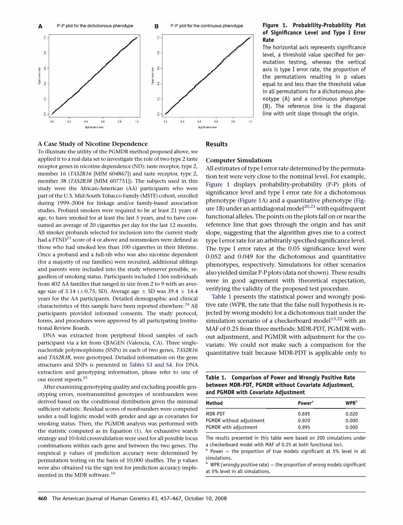
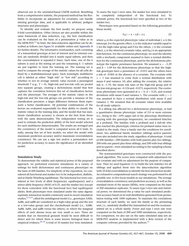
Figure 1. Probability-Probability Plotof Significance Level and Type I ErrorRateThe horizontal axis represents significancelevel, a threshold value specified for per-mutation testing, whereas the verticalaxis is type I error rate, the proportion ofthe permutations resulting in p valuesequal to and less than the threshold valuein all permutations for a dichotomous phe-notype (A) and a continuous phenotype(B). The reference line is the diagonalline with unit slope through the origin.

A Case Study of Nicotine DependenceTo illustrate the utility of the PGMDR method proposed above, we

applied it to a real data set to investigate the role of two type 2 taste

receptor genes in nicotine dependence (ND): taste receptor, type 2,

member 16 (TAS2R16 [MIM 604867]) and taste receptor, type 2,

member 38 (TAS2R38 [MIM 607751]). The subjects used in this

study were the African-American (AA) participants who were

part of the U.S. Mid-South Tobacco Family (MSTF) cohort, enrolled

during 1999–2004 for linkage and/or family-based association

studies. Proband smokers were required to be at least 21 years of

age, to have smoked for at least the last 5 years, and to have con-

sumed an average of 20 cigarettes per day for the last 12 months.

All smoker probands selected for inclusion into the current study

had a FTND23 score of 4 or above and nonsmokers were defined as

those who had smoked less than 100 cigarettes in their lifetime.

Once a proband and a full-sib who was also nicotine dependent

(for a majority of our families) were recruited, additional siblings

and parents were included into the study whenever possible, re-

gardless of smoking status. Participants included 1366 individuals

from 402 AA families that ranged in size from 2 to 9 with an aver-

age size of 3.14 (50.75; SD). Average age 5 SD was 39.4 5 14.4

years for the AA participants. Detailed demographic and clinical

characteristics of this sample have been reported elsewhere.24 All

participants provided informed consents. The study protocol,

forms, and procedures were approved by all participating Institu-

tional Review Boards.

DNA was extracted from peripheral blood samples of each

participant via a kit from QIAGEN (Valencia, CA). Three single-

nucleotide polymorphisms (SNPs) in each of two genes, TAS2R16

and TAS2R38, were genotyped. Detailed information on the gene

structures and SNPs is presented in Tables S3 and S4. For DNA

extraction and genotyping information, please refer to one of

our recent reports.25

After examining genotyping quality and excluding possible gen-

otyping errors, nontransmitted genotypes of nonfounders were

derived based on the conditional distribution given the minimal

sufficient statistic. Residual scores of nonfounders were computed

under a null logistic model with gender and age as covariates for

smoking status. Then, the PGMDR analysis was performed with

the statistic computed as in Equation (1). An exhaustive search

strategy and 10-fold crossvalidation were used for all possible locus

combinations within each gene and between the two genes. The

empirical p values of prediction accuracy were determined by

permutation testing on the basis of 10,000 shuffles. The p values

were also obtained via the sign test for prediction accuracy imple-

mented in the MDR software.10

460 The American Journal of Human Genetics 83, 457–467, Octobe

Results

Computer Simulations

All estimates of type I error rate determined by the permuta-

tion test were very close to the nominal level. For example,

Figure 1 displays probability-probability (P-P) plots of

significance level and type I error rate for a dichotomous

phenotype (Figure 1A) and a quantitative phenotype (Fig-

ure 1B) under an antidiagonal model20,21 with equifrequent

functional alleles. The points on the plots fall on or near the

reference line that goes through the origin and has unit

slope, suggesting that the algorithm gives rise to a correct

type I error rate for an arbitrarily specified significance level.

The type I error rates at the 0.05 significance level were

0.052 and 0.049 for the dichotomous and quantitative

phenotypes, respectively. Simulations for other scenarios

also yielded similar P-P plots (data not shown). These results

were in good agreement with theoretical expectation,

verifying the validity of the proposed test procedure.

Table 1 presents the statistical power and wrongly posi-

tive rate (WPR, the rate that the false null hypothesis is re-

jected by wrong models) for a dichotomous trait under the

simulation scenario of a checkerboard model13,22 with an

MAF of 0.25 from three methods: MDR-PDT, PGMDR with-

out adjustment, and PGMDR with adjustment for the co-

variate. We could not make such a comparison for the

quantitative trait because MDR-PDT is applicable only to

Table 1. Comparison of Power and Wrongly Positive Ratebetween MDR-PDT, PGMDR without Covariate Adjustment,and PGMDR with Covariate Adjustment

Method Powera WPRb

MDR-PDT 0.695 0.020

PGMDR without adjustment 0.920 0.000

PGMDR with adjustment 0.995 0.000

The results presented in this table were based on 200 simulations under

a checkerboard model with MAF of 0.25 at both functional loci.a Power ¼ the proportion of true models significant at 5% level in all

simulations.b WPR (wrongly positive rate)¼ the proportion of wrong models significant

at 5% level in all simulations.

r 10, 2008

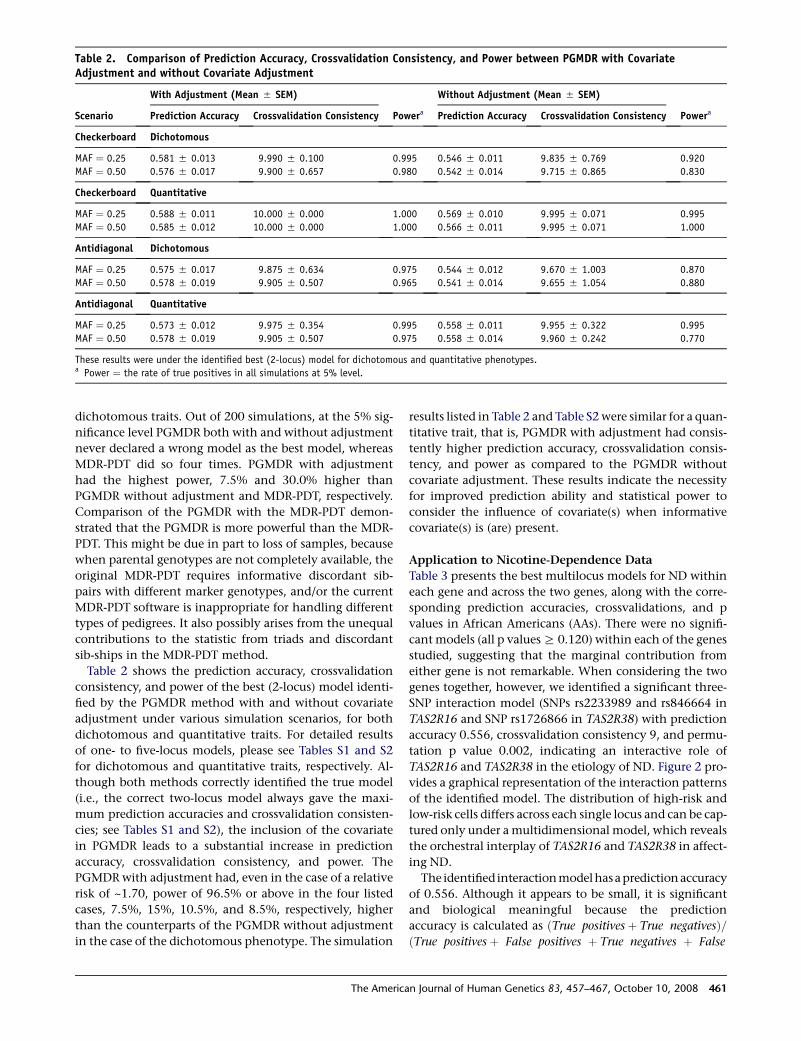
Table 2. Comparison of Prediction Accuracy, Crossvalidation Consistency, and Power between PGMDR with CovariateAdjustment and without Covariate Adjustment

Scenario

With Adjustment (Mean 5 SEM)

Powera

Without Adjustment (Mean 5 SEM)

PoweraPrediction Accuracy Crossvalidation Consistency Prediction Accuracy Crossvalidation Consistency

Checkerboard Dichotomous

MAF ¼ 0.25 0.581 5 0.013 9.990 5 0.100 0.995 0.546 5 0.011 9.835 5 0.769 0.920

MAF ¼ 0.50 0.576 5 0.017 9.900 5 0.657 0.980 0.542 5 0.014 9.715 5 0.865 0.830

Checkerboard Quantitative

MAF ¼ 0.25 0.588 5 0.011 10.000 5 0.000 1.000 0.569 5 0.010 9.995 5 0.071 0.995

MAF ¼ 0.50 0.585 5 0.012 10.000 5 0.000 1.000 0.566 5 0.011 9.995 5 0.071 1.000

Antidiagonal Dichotomous

MAF ¼ 0.25 0.575 5 0.017 9.875 5 0.634 0.975 0.544 5 0.012 9.670 5 1.003 0.870

MAF ¼ 0.50 0.578 5 0.019 9.905 5 0.507 0.965 0.541 5 0.014 9.655 5 1.054 0.880

Antidiagonal Quantitative

MAF ¼ 0.25 0.573 5 0.012 9.975 5 0.354 0.995 0.558 5 0.011 9.955 5 0.322 0.995

MAF ¼ 0.50 0.578 5 0.019 9.905 5 0.507 0.975 0.558 5 0.014 9.960 5 0.242 0.770

These results were under the identified best (2-locus) model for dichotomous and quantitative phenotypes.a Power ¼ the rate of true positives in all simulations at 5% level.

dichotomous traits. Out of 200 simulations, at the 5% sig-

nificance level PGMDR both with and without adjustment

never declared a wrong model as the best model, whereas

MDR-PDT did so four times. PGMDR with adjustment

had the highest power, 7.5% and 30.0% higher than

PGMDR without adjustment and MDR-PDT, respectively.

Comparison of the PGMDR with the MDR-PDT demon-

strated that the PGMDR is more powerful than the MDR-

PDT. This might be due in part to loss of samples, because

when parental genotypes are not completely available, the

original MDR-PDT requires informative discordant sib-

pairs with different marker genotypes, and/or the current

MDR-PDT software is inappropriate for handling different

types of pedigrees. It also possibly arises from the unequal

contributions to the statistic from triads and discordant

sib-ships in the MDR-PDT method.

Table 2 shows the prediction accuracy, crossvalidation

consistency, and power of the best (2-locus) model identi-

fied by the PGMDR method with and without covariate

adjustment under various simulation scenarios, for both

dichotomous and quantitative traits. For detailed results

of one- to five-locus models, please see Tables S1 and S2

for dichotomous and quantitative traits, respectively. Al-

though both methods correctly identified the true model

(i.e., the correct two-locus model always gave the maxi-

mum prediction accuracies and crossvalidation consisten-

cies; see Tables S1 and S2), the inclusion of the covariate

in PGMDR leads to a substantial increase in prediction

accuracy, crossvalidation consistency, and power. The

PGMDR with adjustment had, even in the case of a relative

risk of ~1.70, power of 96.5% or above in the four listed

cases, 7.5%, 15%, 10.5%, and 8.5%, respectively, higher

than the counterparts of the PGMDR without adjustment

in the case of the dichotomous phenotype. The simulation

The Ameri

results listed in Table 2 and Table S2 were similar for a quan-

titative trait, that is, PGMDR with adjustment had consis-

tently higher prediction accuracy, crossvalidation consis-

tency, and power as compared to the PGMDR without

covariate adjustment. These results indicate the necessity

for improved prediction ability and statistical power to

consider the influence of covariate(s) when informative

covariate(s) is (are) present.

Application to Nicotine-Dependence Data

Table 3 presents the best multilocus models for ND within

each gene and across the two genes, along with the corre-

sponding prediction accuracies, crossvalidations, and p

values in African Americans (AAs). There were no signifi-

cant models (all p values R 0.120) within each of the genes

studied, suggesting that the marginal contribution from

either gene is not remarkable. When considering the two

genes together, however, we identified a significant three-

SNP interaction model (SNPs rs2233989 and rs846664 in

TAS2R16 and SNP rs1726866 in TAS2R38) with prediction

accuracy 0.556, crossvalidation consistency 9, and permu-

tation p value 0.002, indicating an interactive role of

TAS2R16 and TAS2R38 in the etiology of ND. Figure 2 pro-

vides a graphical representation of the interaction patterns

of the identified model. The distribution of high-risk and

low-risk cells differs across each single locus and can be cap-

tured only under a multidimensional model, which reveals

the orchestral interplay of TAS2R16 and TAS2R38 in affect-

ing ND.

The identified interaction modelhasa prediction accuracy

of 0.556. Although it appears to be small, it is significant

and biological meaningful because the prediction

accuracy is calculated as ðTrue positivesþ True negativesÞ=ðTrue positivesþ False positives þ True negatives þ False

can Journal of Human Genetics 83, 457–467, October 10, 2008 461

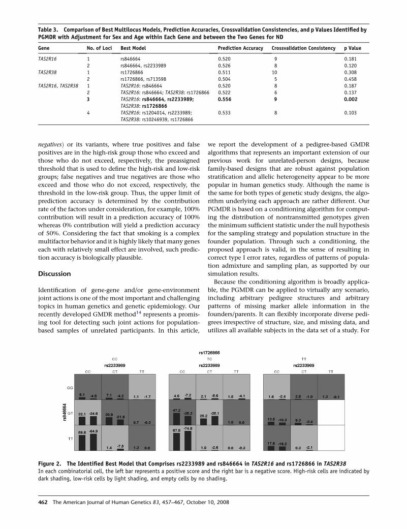
Table 3. Comparison of Best Multilocus Models, Prediction Accuracies, Crossvalidation Consistencies, and p Values Identified byPGMDR with Adjustment for Sex and Age within Each Gene and between the Two Genes for ND

Gene No. of Loci Best Model Prediction Accuracy Crossvalidation Consistency p Value

TAS2R16 1 rs846664 0.520 9 0.181

2 rs846664, rs2233989 0.526 8 0.120

TAS2R38 1 rs1726866 0.511 10 0.308

2 rs1726866, rs713598 0.504 5 0.458

TAS2R16, TAS2R38 1 TAS2R16: rs846664 0.520 8 0.187

2 TAS2R16: rs846664; TAS2R38: rs1726866 0.522 6 0.137

3 TAS2R16: rs846664, rs2233989; 0.556 9 0.002TAS2R38: rs1726866

4 TAS2R16: rs1204014, rs2233989; 0.533 8 0.103

TAS2R38: rs10246939, rs1726866

negativesÞ or its variants, where true positives and false

positives are in the high-risk group those who exceed and

those who do not exceed, respectively, the preassigned

threshold that is used to define the high-risk and low-risk

groups; false negatives and true negatives are those who

exceed and those who do not exceed, respectively, the

threshold in the low-risk group. Thus, the upper limit of

prediction accuracy is determined by the contribution

rate of the factors under consideration, for example, 100%

contribution will result in a prediction accuracy of 100%

whereas 0% contribution will yield a prediction accuracy

of 50%. Considering the fact that smoking is a complex

multifactor behavior and it is highly likely that many genes

each with relatively small effect are involved, such predic-

tion accuracy is biologically plausible.

Discussion

Identification of gene-gene and/or gene-environment

joint actions is one of the most important and challenging

topics in human genetics and genetic epidemiology. Our

recently developed GMDR method14 represents a promis-

ing tool for detecting such joint actions for population-

based samples of unrelated participants. In this article,

we report the development of a pedigree-based GMDR

algorithms that represents an important extension of our

previous work for unrelated-person designs, because

family-based designs that are robust against population

stratification and allelic heterogeneity appear to be more

popular in human genetics study. Although the name is

the same for both types of genetic study designs, the algo-

rithm underlying each approach are rather different. Our

PGMDR is based on a conditioning algorithm for comput-

ing the distribution of nontransmitted genotypes given

the minimum sufficient statistic under the null hypothesis

for the sampling strategy and population structure in the

founder population. Through such a conditioning, the

proposed approach is valid, in the sense of resulting in

correct type I error rates, regardless of patterns of popula-

tion admixture and sampling plan, as supported by our

simulation results.

Because the conditioning algorithm is broadly applica-

ble, the PGMDR can be applied to virtually any scenario,

including arbitrary pedigree structures and arbitrary

patterns of missing marker allele information in the

founders/parents. It can flexibly incorporate diverse pedi-

grees irrespective of structure, size, and missing data, and

utilizes all available subjects in the data set of a study. For

Figure 2. The Identified Best Model that Comprises rs2233989 and rs846664 in TAS2R16 and rs1726866 in TAS2R38In each combinatorial cell, the left bar represents a positive score and the right bar is a negative score. High-risk cells are indicated bydark shading, low-risk cells by light shading, and empty cells by no shading.

462 The American Journal of Human Genetics 83, 457–467, October 10, 2008

example, concordant sibs, unaffected offspring in a family,

and subjects with missing genotypes, which are often

encountered in real data sets but are not useful for the

MDR-PDT and the original MDR, do inform our pedigree-

based statistic. Without discarding any samples at hand,

the proposed method is able to take full advantage of the

whole data set and extract more genetic information. Our

simulation comparisons between the PGMDR and the

MDR-PDT algorithms and the ND data set demonstrate

that our proposed algorithm is more powerful, likely

benefiting from capitalizing on more of the data.

The proposed approach, in nature, represents a compre-

hensive statistical framework. Within this framework, we

can use a broad category of test statistics that measure the

covariance between the transmission of genotype and

a function of the phenotype, such as the score-like

statistics for quasilikelihood models, so that any kind of

phenotype and multiallelic markers may be examined.

In contrast to the MDR-PDT and the MDR methods that

are restricted to the context of discordant sib-ships and di-

chotomous traits, the proposed approach is flexible

enough to handle diverse phenotypes, categorical, cen-

sored, or continuous. The extension to multivariate phe-

notypes is also straightforward. Furthermore, one of the

most important advantages of the proposed approach is

that it allows adjustment for covariates so that it can in-

crease predictive ability and statistical power by control-

ling confounding effects of covariates. Both the simula-

tions and the application to the ND data set attest to

the claim that our method can increase prediction accu-

racy and statistical power by inclusion of informative

covariates.

Under this broad framework, available combinatory

approaches can be thought of as special cases in various

scenarios. The proposed method is an extension to fam-

ily-based designs of our recent GMDR14 that itself is a gen-

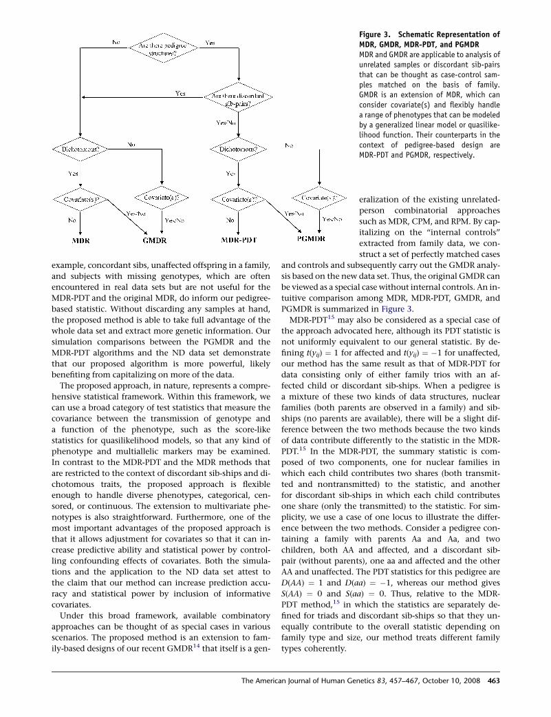
Figure 3. Schematic Representation ofMDR, GMDR, MDR-PDT, and PGMDRMDR and GMDR are applicable to analysis ofunrelated samples or discordant sib-pairsthat can be thought as case-control sam-ples matched on the basis of family.GMDR is an extension of MDR, which canconsider covariate(s) and flexibly handlea range of phenotypes that can be modeledby a generalized linear model or quasilike-lihood function. Their counterparts in thecontext of pedigree-based design areMDR-PDT and PGMDR, respectively.

eralization of the existing unrelated-

person combinatorial approaches

such as MDR, CPM, and RPM. By cap-

italizing on the ‘‘internal controls’’

extracted from family data, we con-

struct a set of perfectly matched cases

and controls and subsequently carry out the GMDR analy-

sis based on the new data set. Thus, the original GMDR can

be viewed as a special case without internal controls. An in-

tuitive comparison among MDR, MDR-PDT, GMDR, and

PGMDR is summarized in Figure 3.

MDR-PDT15 may also be considered as a special case of

the approach advocated here, although its PDT statistic is

not uniformly equivalent to our general statistic. By de-

fining t(yij) ¼ 1 for affected and t(yij) ¼ �1 for unaffected,

our method has the same result as that of MDR-PDT for

data consisting only of either family trios with an af-

fected child or discordant sib-ships. When a pedigree is

a mixture of these two kinds of data structures, nuclear

families (both parents are observed in a family) and sib-

ships (no parents are available), there will be a slight dif-

ference between the two methods because the two kinds

of data contribute differently to the statistic in the MDR-

PDT.15 In the MDR-PDT, the summary statistic is com-

posed of two components, one for nuclear families in

which each child contributes two shares (both transmit-

ted and nontransmitted) to the statistic, and another

for discordant sib-ships in which each child contributes

one share (only the transmitted) to the statistic. For sim-

plicity, we use a case of one locus to illustrate the differ-

ence between the two methods. Consider a pedigree con-

taining a family with parents Aa and Aa, and two

children, both AA and affected, and a discordant sib-

pair (without parents), one aa and affected and the other

AA and unaffected. The PDT statistics for this pedigree are

D(AA) ¼ 1 and D(aa) ¼ �1, whereas our method gives

S(AA) ¼ 0 and S(aa) ¼ 0. Thus, relative to the MDR-

PDT method,15 in which the statistics are separately de-

fined for triads and discordant sib-ships so that they un-

equally contribute to the overall statistic depending on

family type and size, our method treats different family

types coherently.

The American Journal of Human Genetics 83, 457–467, October 10, 2008 463

The proposed approach has a unified framework for

coherently handling different family types. Under this

concept, each nonfounder that informs the test statistic

has a set of nontransmitted genotypes as a control. Un-

like the MDR-PDT where there exists an intrinsic diffi-

culty for permuting within larger extended pedigrees

with general structures,15 a permutation test is always

easy to perform for pedigrees with arbitrary structure

and arbitrary size by randomly flipping the transmitted

and nontransmitted genotype sets in a pedigree and

thereby preserving in each permuted data set the possible

nonindependence of transmissions across markers and

across nonfounders.

The general statistical framework developed here also

offers great flexibility in the use of different phenotype

coding strategies. Although any phenotype-coding strat-

egy is valid and results in correct type I error rates under

the null hypothesis, some do provide more efficient and/

or sensitive measures of association under the alternative

and the choice of an appropriate coding strategy can sub-

stantially increase test power. Optimal choices for coding

depend on the study design (e.g., only trios in which the

offspring is affected versus a sample that also includes

unaffected persons) and possibly unknown parameters

(e.g., prevalence rate, relative risk, and allele frequency).

We may obtain an approximately optimal coding based

on prior knowledge of the disease. Power simulations

may also provide guideline for the appropriate choice

based on hypothetical scenarios in which the real parame-

ters potentially fall, although it may be difficult to deter-

mine the real parameters exactly.

The illustrative example demonstrates that the pro-

posed method can unveil cryptic interactions between

the genes TAS2R16 and TAS2R38. Biologically, bitterness

perception serves as a warning system that leads humans

to reject substances that are potentially toxic.26 Human

taste receptors, including type 2 taste receptors (TAS2Rs),

are expressed primarily in taste buds of gustatory papillae

on the tongue surface and palate epithelia. Genetic stud-

ies point to diverse taste perception of bitter substances,

as well as overall oral sensitivity, among individuals and

between ethnic groups partly because of polymorphisms

in taste receptor genes.27 For example, several SNPs

within the TAS2R genes, which encode TAS2R proteins,

can characterize ‘‘tasters’’ and ‘‘nontasters.’’28 Polymor-

phisms in TAS2R genes are implicated in variations of

orally related behaviors, including alcohol29 and nico-

tine30 consumption and dependence. Recently, we found

that several polymorphisms in TAS2R genes are poten-

tially implicated in ND 25. Bitter taste receptor genes are

heterogeneously expressed in taste receptor cells and

TAS2Rs compete with each other for shared cellular re-

sources, from biosynthesis to signaling and ultimately

to turnover.31 This indicates that the significant

statistical interaction detected in this study may represent

a biological interaction between TAS2R genes. As illus-

trated in this study, the role of TAS2R genes in the etiol-

464 The American Journal of Human Genetics 83, 457–467, Octobe

ogy of ND is complex; further study is required to assess

functional details.

Appendix A: Algorithm for Computation

of the Conditional Distribution

of Nontransmitted Genotypes

The key step involved in the proposed approach is the

computation of the conditional distribution of nontrans-

mitted genotypes given the minimal sufficient statistic

under the null hypothesis for the phenotype distribution

and the parental genotype distribution. When both paren-

tal genotypes are known, the observed phenotypes in all

family members and the parental genotypes constitute

the minimal sufficient statistic, and the conditional distri-

bution of nontransmitted genotypes is straightforward.

When parental genotype data are not completely available,

however, the conditional distribution of the nontransmit-

ted genotype of an offspring is not immediately obvious.

In this appendix, we present an algorithm for computing

the conditional distribution of nontransmitted genotypes

given the minimal sufficient statistics. To some extent,

this algorithm represents an extension of the approach

proposed by Rabinowitz and Laird.16 The difference

between the two is that we consider here the conditional

distribution of nontransimitted genotypes rather than

that of transmitted genotypes as is done in Rabinowitz

and Laird.16 For each pedigree, the observed genotypes of

nonfounders constitute the set of transmitted genotypes

whereas their nontransmitted counterparts form a set of

nontransmitted genotypes. Under the null hypothesis,

each parent is equally likely to transmit either of her/his

marker alleles and all these parental transmissions are

considered to be independent. Thus, if we do not need to

consider the compatibility of nontransmitted genotypes

with the observed genotypes, a set of transmitted geno-

types can be viewed as one of the plausible realizations

of nontransmitted genotypes and the conditional distribu-

tion of transmitted genotypes derived by Rabinowitz and

Laird’s algorithm16 can also represent that of nontransmit-

ted genotypes given the minimal sufficient statistic. Our

algorithm is based on such a concept of equally frequent

transmissions. Both the transmitted and nontransmitted

sets are assumed to come from a hypothetical homogenous

population.

While remaining the framework unaltered in the original

algorithm,16 we define here all observed traits, typed

marker alleles, and a plausible set of nontransmitted alleles

in a pedigree as an outcome for the pedigree, instead of that

consisting of all observed traits and typed marker alleles.

Similar to that of Rabinowitz and Laird,16 the condition

that characterizes the minimal sufficient statistic under

the null hypothesis is that: if two different outcomes

have the same value of the minimal sufficient statistic,

then for any pattern of founders’ genotypes, either the con-

ditional probabilities of two outcomes given the pattern of

r 10, 2008

founders’ genotypes are both equal to zero, or the ratio of

the conditional probabilities of the outcomes is invariant

to the choice of the pattern of founders’ genotypes. As

pointed out by Rabinowitz and Laird,16 such a minimal

sufficient statistic is not represented as a particular function

of the data, but rather as a partition of the sample space.

The general steps involved in the algorithm for deriving

the minimal sufficient statistic and computing the condi-

tional distribution of nontransmitted genotypes in a pedi-

gree (a nuclear family is a special case) can be summarized

as follows.

(1) Find all the patterns of founder (parent in a nuclear

family) marker genotypes that are compatible with the

observed genotypes.

(2) For each of the patterns of compatible founder

marker genotypes obtained in step (1), find the set of

compatible patterns of nontransmitted genotypes in the

pedigree. Find the subset of these compatible patterns

that, together with the observed nonfounders’ genotypes,

have exactly the same compatible patterns of founders’

genotypes as the observed nonfounders’ genotypes.

(3) Find the subset of these compatible patterns found in

step (2) that are compatible with all observed founder and

nonfounder genotypes. Some of the nontransmitted geno-

types may be fixed in this subset whereas the others may

not. Below we call them fixed nontransmitted genotypes

and nonfixed nontransmitted genotypes, respectively.

(4) For every pattern of compatible founder genotypes

found in step (1) and for every pattern of nontransmitted

genotypes in the subset found in step (3), compute the

ratio of the geometrical mean of the conditional probabil-

ity of the observed genotypes (pseudo nontransmitted

genotypes) to that of the conditional probability of the

nonfixed nontransmitted genotypes in the subset given

the pattern of founders’ genotypes.

(5) For some patterns of nontransmitted genotypes in

the subset found in step (3), the ratios found in step (4)

will be the same for all of the compatible patterns of

founders’ genotypes found in step (1).

(6) The conditional distribution is found by arbitrarily

choosing any of the compatible patterns of founder geno-

types found in step (1) and computing the conditional

probabilities of the patterns of nontransmitted genotypes

given the chosen pattern of founders’ genotypes and given

the set of patterns of nontransmitted genotypes described

in step (5).

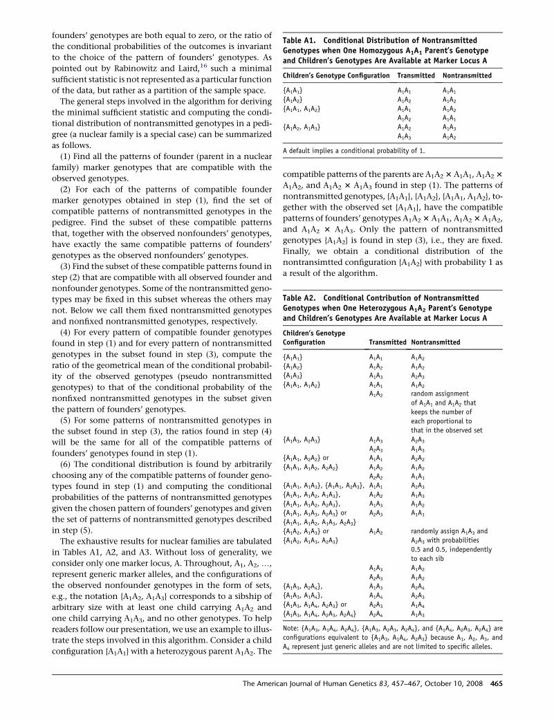
The exhaustive results for nuclear families are tabulated

in Tables A1, A2, and A3. Without loss of generality, we

consider only one marker locus, A. Throughout, A1, A2, .,

represent generic marker alleles, and the configurations of

the observed nonfounder genotypes in the form of sets,

e.g., the notation {A1A2, A1A3} corresponds to a sibship of

arbitrary size with at least one child carrying A1A2 and

one child carrying A1A3, and no other genotypes. To help

readers follow our presentation, we use an example to illus-

trate the steps involved in this algorithm. Consider a child

configuration {A1A1} with a heterozygous parent A1A2. The

The Ameri

compatible patterns of the parents are A1A2 3 A1A1, A1A2 3

A1A2, and A1A2 3 A1A3 found in step (1). The patterns of

nontransmitted genotypes, {A1A1}, {A1A2}, {A1A1, A1A2}, to-

gether with the observed set {A1A1}, have the compatible

patterns of founders’ genotypes A1A2 3 A1A1, A1A2 3 A1A2,

and A1A2 3 A1A3. Only the pattern of nontransmitted

genotypes {A1A2} is found in step (3), i.e., they are fixed.

Finally, we obtain a conditional distribution of the

nontransimtted configuration {A1A2} with probability 1 as

a result of the algorithm.

Table A1. Conditional Distribution of NontransmittedGenotypes when One Homozygous A1A1 Parent’s Genotypeand Children’s Genotypes Are Available at Marker Locus A

Children’s Genotype Configuration Transmitted Nontransmitted

{A1A1} A1A1 A1A1

{A1A2} A1A2 A1A2

{A1A1, A1A2} A1A1 A1A2

A1A2 A1A1

{A1A2, A1A3} A1A2 A1A3

A1A3 A1A2

A default implies a conditional probability of 1.

Table A2. Conditional Contribution of NontransmittedGenotypes when One Heterozygous A1A2 Parent’s Genotypeand Children’s Genotypes Are Available at Marker Locus A

Children’s GenotypeConfiguration Transmitted Nontransmitted

{A1A1} A1A1 A1A2

{A1A2} A1A2 A1A2

{A1A3} A1A3 A2A3

{A1A1, A1A2} A1A1 A1A2

A1A2 random assignment

of A1A1 and A1A2 that

keeps the number of

each proportional to

that in the observed set

{A1A3, A2A3} A1A3 A2A3

A2A3 A1A3

{A1A1, A2A2} or A1A1 A2A2

{A1A1, A1A2, A2A2} A1A2 A1A2

A2A2 A1A1

{A1A1, A1A3}, {A1A1, A2A3}, A1A1 A2A3

{A1A1, A1A2, A1A3}, A1A2 A1A3

{A1A1, A1A2, A2A3}, A1A3 A1A2

{A1A1, A1A3, A2A3} or A2A3 A1A1

{A1A1, A1A2, A1A3, A2A3}

{A1A2, A1A3} or

{A1A2, A1A3, A2A3}

A1A2 randomly assign A1A3 and

A2A3 with probabilities

0.5 and 0.5, independently

to each sib

A1A3 A1A2

A2A3 A1A2

{A1A3, A2A4}, A1A3 A2A4

{A1A3, A1A4}, A1A4 A2A3

{A1A3, A1A4, A2A3} or A2A3 A1A4

{A1A3, A1A4, A2A3, A2A4} A2A4 A1A3

Note: {A1A3, A1A4, A2A4}, {A1A3, A2A3, A2A4}, and {A1A4, A2A3, A2A4} are

configurations equivalent to {A1A3, A1A4, A2A3} because A1, A2, A3, and

A4 represent just generic alleles and are not limited to specific alleles.

can Journal of Human Genetics 83, 457–467, October 10, 2008 465

Appendix B: A Schematic Illustration

of the Pedigree-Based GMDR Algorithm

We briefly use Figure S1 to illustrate the steps involved in

conducting the pedigree-based GMDR method. Without

loss of generality, we consider here a classic TDT design

in which each family consists of an affected child and

both parents. To focus on exposition of the data-reduction

algorithm, we assume in Figure S1 no covariate and take

t(yij) ¼ 0.5 for affected children, although we can use any

appropriate statistic instead of this, as deemed necessary.

From Equation (1), all the transmitted genotypes in infor-

mative family triads constitute cases whereas the nontrans-

mitted genotypes serve as artificial internal controls, thus

constituting a balanced case-control sample. In Step 1,

the pairs of the transmitted and nontransmitted genotypes

are randomly split into some number of equal parts for

crossvalidation; as an illustration, 10-fold crossvalidation

is used in Figure S1. One subdivision is used as the testing

set and the rest as the independent training set. Then,

Steps 2 through 5 are run for the training set and Step 6

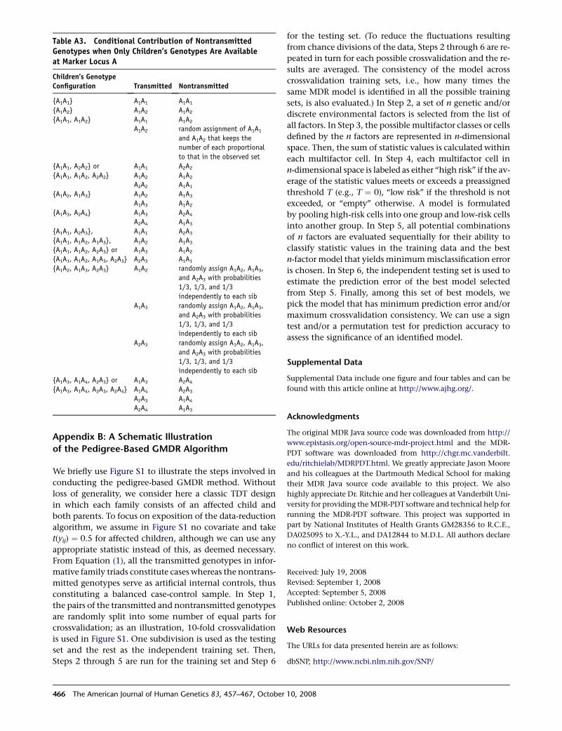
Table A3. Conditional Contribution of NontransmittedGenotypes when Only Children’s Genotypes Are Availableat Marker Locus A

Children’s GenotypeConfiguration Transmitted Nontransmitted

{A1A1} A1A1 A1A1

{A1A2} A1A2 A1A2

{A1A1, A1A2} A1A1 A1A2

A1A2 random assignment of A1A1

and A1A2 that keeps the

number of each proportional

to that in the observed set

{A1A1, A2A2} or A1A1 A2A2

{A1A1, A1A2, A2A2} A1A2 A1A2

A2A2 A1A1

{A1A2, A1A3} A1A2 A1A3

A1A3 A1A2

{A1A3, A2A4} A1A3 A2A4

A2A4 A1A3

{A1A1, A2A3}, A1A1 A2A3

{A1A1, A1A2, A1A3}, A1A2 A1A3

{A1A1, A1A2, A2A3} or A1A3 A1A2

{A1A1, A1A2, A1A3, A2A3} A2A3 A1A1

{A1A2, A1A3, A2A3} A1A2 randomly assign A1A2, A1A3,

and A2A3 with probabilities

1/3, 1/3, and 1/3

independently to each sib

A1A3 randomly assign A1A2, A1A3,

and A2A3 with probabilities

1/3, 1/3, and 1/3

independently to each sib

A2A3 randomly assign A1A2, A1A3,

and A2A3 with probabilities

1/3, 1/3, and 1/3

independently to each sib

{A1A3, A1A4, A2A3} or A1A3 A2A4

{A1A3, A1A4, A2A3, A2A4} A1A4 A2A3

A2A3 A1A4

A2A4 A1A3

466 The American Journal of Human Genetics 83, 457–467, Octobe

for the testing set. (To reduce the fluctuations resulting

from chance divisions of the data, Steps 2 through 6 are re-

peated in turn for each possible crossvalidation and the re-

sults are averaged. The consistency of the model across

crossvalidation training sets, i.e., how many times the

same MDR model is identified in all the possible training

sets, is also evaluated.) In Step 2, a set of n genetic and/or

discrete environmental factors is selected from the list of

all factors. In Step 3, the possible multifactor classes or cells

defined by the n factors are represented in n-dimensional

space. Then, the sum of statistic values is calculated within

each multifactor cell. In Step 4, each multifactor cell in

n-dimensional space is labeled as either ‘‘high risk’’ if the av-

erage of the statistic values meets or exceeds a preassigned

threshold T (e.g., T ¼ 0), ‘‘low risk’’ if the threshold is not

exceeded, or ‘‘empty’’ otherwise. A model is formulated

by pooling high-risk cells into one group and low-risk cells

into another group. In Step 5, all potential combinations

of n factors are evaluated sequentially for their ability to

classify statistic values in the training data and the best

n-factor model that yields minimum misclassification error

is chosen. In Step 6, the independent testing set is used to

estimate the prediction error of the best model selected

from Step 5. Finally, among this set of best models, we

pick the model that has minimum prediction error and/or

maximum crossvalidation consistency. We can use a sign

test and/or a permutation test for prediction accuracy to

assess the significance of an identified model.

Supplemental Data

Supplemental Data include one figure and four tables and can be

found with this article online at http://www.ajhg.org/.

Acknowledgments

The original MDR Java source code was downloaded from http://

www.epistasis.org/open-source-mdr-project.html and the MDR-

PDT software was downloaded from http://chgr.mc.vanderbilt.

edu/ritchielab/MDRPDT.html. We greatly appreciate Jason Moore

and his colleagues at the Dartmouth Medical School for making

their MDR Java source code available to this project. We also

highly appreciate Dr. Ritchie and her colleagues at Vanderbilt Uni-

versity for providing the MDR-PDT software and technical help for

running the MDR-PDT software. This project was supported in

part by National Institutes of Health Grants GM28356 to R.C.E.,

DA025095 to X.-Y.L., and DA12844 to M.D.L. All authors declare

no conflict of interest on this work.

Received: July 19, 2008

Revised: September 1, 2008

Accepted: September 5, 2008

Published online: October 2, 2008

Web Resources

The URLs for data presented herein are as follows:

dbSNP, http://www.ncbi.nlm.nih.gov/SNP/

r 10, 2008

Ensembl Human, http://www.ensembl.org/Homo_sapiens/

Entrez Gene, http://www.ncbi.nlm.nih.gov/entrez/query.

fcgi?db¼gene

Epistasis.org, Computational Genetics Laboratory, http://www.

epistasis.org/

Epistasis Blog, http://compgen.blogspot.com/2006/05/

mdr-applications.html

MDR-PDT software, http://chgr.mc.vanderbilt.edu/ritchielab/

MDRPDT.html

Online Mendelian Inheritance in Man (OMIM), http://www.ncbi.

nlm.nih.gov/Omim/

PGMDR program, http://www.healthsystem.virginia.edu/

internet/addiction-genomics

References

1. Hunter, D.J. (2005). Gene-environment interactions in

human diseases. Nat. Rev. Genet. 6, 287–298.

2. Tong, A.H.Y., Lesage, G., Bader, G.D., Ding, H.M., Xu, H., Xin,

X.F., Young, J., Berriz, G.F., Brost, R.L., Chang, M., et al. (2004).

Global mapping of the yeast genetic interaction network.

Science 303, 808–813.

3. Segre, D., Deluna, A., Church, G.M., and Kishony, R. (2005).

Modular epistasis in yeast metabolism. Nat. Genet. 37, 77–83.

4. Lander, E.S., and Schork, N.J. (1994). Genetic dissection of

complex traits. Science 265, 2037–2048.

5. Carlborg, O., and Haley, C.S. (2004). Epistasis: Too often ne-

glected in complex trait studies? Nat. Rev. Genet. 5, 618–625.

6. Barton, N.H., and Keightley, P.D. (2002). Understanding quan-

titative genetic variation. Nat. Rev. Genet. 3, 11–21.

7. Flint, J., and Mott, R. (2001). Finding the molecular basis of

quantitative traits: Successes and pitfalls. Nat. Rev. Genet. 2,

437–445.

8. Kroymann, J., and Mitchell-Olds, T. (2005). Epistasis and

balanced polymorphism influencing complex trait variation.

Nature 435, 95–98.

9. Ritchie, M.D., Hahn, L.W., Roodi, N., Bailey, L.R., Dupont,

W.D., Parl, F.F., and Moore, J.H. (2001). Multifactor-dimen-

sionality reduction reveals high-order interactions among

estrogen-metabolism genes in sporadic breast cancer. Am. J.

Hum. Genet. 69, 138–147.

10. Hahn, L.W., Ritchie, M.D., and Moore, J.H. (2003). Multifactor

dimensionality reduction software for detecting gene-gene

and gene-environment interactions. Bioinformatics 19, 376–

382.

11. Moore, J.H., Gilbert, J.C., Tsai, C.T., Chiang, F.T., Holden, T.,

Barney, N., and White, B.C. (2006). A flexible computational

framework for detecting, characterizing, and interpreting

statistical patterns of epistasis in genetic studies of human

disease susceptibility. J. Theor. Biol. 241, 252–261.

12. Nelson, M.R., Kardia, S.L., Ferrell, R.E., and Sing, C.F. (2001). A

combinatorial partitioning method to identify multilocus

genotypic partitions that predict quantitative trait variation.

Genome Res. 11, 458–470.

13. Culverhouse, R., Klein, T., and Shannon, W. (2004). Detecting

epistatic interactions contributing to quantitative traits.

Genet. Epidemiol. 27, 141–152.

14. Lou, X.Y., Chen, G.B., Yan, L., Ma, J.Z., Zhu, J., Elston, R.C.,

and Li, M.D. (2007). A generalized combinatorial approach

for detecting gene-by-gene and gene-by-environment interac-

tions with application to nicotine dependence. Am. J. Hum.

Genet. 80, 1125–1137.

The Americ

15. Martin, E.R., Ritchie, M.D., Hahn, L., Kang, S., and Moore, J.H.

(2006). A novel method to identify gene-gene effects in

nuclear families: The MDR-PDT. Genet. Epidemiol. 30,

111–123.

16. Rabinowitz, D., and Laird, N. (2000). A unified approach to

adjusting association tests for population admixture with

arbitrary pedigree structure and arbitrary missing marker

information. Hum. Hered. 50, 211–223.

17. Nelder, J.A., and Wedderbu, R.W. (1972). Generalized linear

models. J. R. Stat. Soc. [Ser A] 135, 370–384.

18. Wedderburn, R.W.M. (1974). Quasi-likelihood functions,

generalized linear-models, and Gauss-Newton method. Bio-

metrika 61, 439–447.

19. McCullagh, P. (1983). Quasi-likelihood functions. Ann. Stat.

11, 59–67.

20. Frankel, W.N., and Schork, N.J. (1996). Who’s afraid of epista-

sis? Nat. Genet. 14, 371–373.

21. Williams, S.M., Haines, J.L., and Moore, J.H. (2004). The use of

animal models in the study of complex disease: All else is

never equal or why do so many human studies fail to replicate

animal findings? Bioessays 26, 170–179.

22. Moore, J.H., and Williams, S.M. (2005). Traversing the

conceptual divide between biological and statistical epistasis:

systems biology and a more modern synthesis. Bioessays 27,

637–646.

23. Heatherton, T.F., Kozlowski, L.T., Frecker, R.C., and Fager-

strom, K.O. (1991). The Fagerstrom Test for nicotine depen-

dence: A revision of the Fagerstrom Tolerance Questionnaire.

Br. J. Addict. 86, 1119–1127.

24. Li, M.D., Payne, T.J., Ma, J.Z., Lou, X.Y., Zhang, D., Dupont,

R.T., Crews, K.M., Somes, G., Williams, N.J., and Elston, R.C.

(2006). A genomewide search finds major susceptibility loci

for nicotine dependence on chromosome 10 in African Amer-

icans. Am. J. Hum. Genet. 79, 745–751.

25. Mangold, J.E., Payne, T.J., Ma, J.Z., Chen, G., and Li, M.D.

(2008). Bitter taste receptor gene polymorphisms are an im-

portant factor in the development of nicotine dependence

in African Americans. J. Med. Genet. 45, 578–582.

26. Glendinning, J.I. (1994). Is the bitter rejection response

always adaptive? Physiol. Behav. 56, 1217–1227.

27. Reed, D.R., Tanaka, T., and McDaniel, A.H. (2006). Diverse

tastes: Genetics of sweet and bitter perception. Physiol. Behav.

88, 215–226.

28. Kim, U.K., Jorgenson, E., Coon, H., Leppert, M., Risch, N., and

Drayna, D. (2003). Positional cloning of the human quantita-

tive trait locus underlying taste sensitivity to phenylthiocarba-

mide. Science 299, 1221–1225.

29. Hinrichs, A.L., Wang, J.C., Bufe, B., Kwon, J.M., Budde, J., Al-

len, R., Bertelsen, S., Evans, W., Dick, D., Rice, J., et al. (2006).

Functional variant in a bitter-taste receptor (hTAS2R16) influ-

ences risk of alcohol dependence. Am. J. Hum. Genet. 78,

103–111.

30. Cannon, D.S., Baker, T.B., Piper, M.E., Scholand, M.B., Law-

rence, D.L., Drayna, D.T., McMahon, W.M., Villegas, G.M.,

Caton, T.C., Coon, H., et al. (2005). Associations between

phenylthiocarbamide gene polymorphisms and cigarette

smoking. Nicotine Tob. Res. 7, 853–858.

31. Behrens, M., Foerster, S., Staehler, F., Raguse, J.D., and Meyer-

hof, W. (2007). Gustatory expression pattern of the human

TAS2R bitter receptor gene family reveals a heterogenous pop-

ulation of bitter responsive taste receptor cells. J. Neurosci. 27,

12630–12640.

an Journal of Human Genetics 83, 457–467, October 10, 2008 467