A Combinatorial Auction with Equilibrium Price Selection

DEGREE PROJECT, IN SOFTWARE ENGINEERING OF DISTRIBUTED SYSTEMS, SECOND LEVEL

STOCKHOLM, SWEDEN 2015

A Combinatorial Auction withEquilibrium Price Selection

KIRIL VIDELOV

KTH ROYAL INSTITUTE OF TECHNOLOGY

INFORMATION AND COMMUNICATION TECHNOLOGY

S

Abstract

Financial markets use auctions to provide accurate liquidity snapshots for traded instru-ments. Combination orders, such as time spreads require the atomic trading of morethan one security contract. In order to auction such complex order types, a new design,which considers all contingent instruments simultaneously, is required.This work develops an optimization model and a software implementation of the dual-sided multi-unit combinatorial auction problem. The optimization objective is findingan equilibrium price vector and a winner selection such that the auction turnover ismaximized.The auction requirements are modeled as a discrete optimization problem, suitable forstandard integer programming solvers. The model’s correctness and tractability aretested using synthetically generated orders as well as real market data.Test results with both synthetic and authentic orders produced equilibrium prices within3% of the expected instrument valuations, using closing prices as a benchmark, indicat-ing high accuracy of the solutions. The use of combinatorial auctions exposes greaterliquidity and overall turnover, both valuable to exchanges that receive large numbers ofcombination orders.

Keywords

Combinatorial auction, Equilibrium price, Discrete optimization

Acknowledgements

I would like to thank the team at Cinnober Financial Technology for welcoming this thesiswork as well as for creating such an inspiring and challenging working environment. I givespecial thanks and my deepest gratitude to my industry supervisor Hannes Edvardson -this thesis would not have been possible without his guidance and expertise. His insightfulcomments were thought provoking and helped me maintain the right focus while hispatience and support have been invaluable to me throughout the process.I am grateful to Ola Bergefall and Martin Bolmstrand for the numerous rewardingdiscussions as well as for their practical advice.

Additionally, I would like to extend my gratitude towards Prof. Anne Håkansson andProf. Mihhail Matskin from the School of Information And Communication Technologyat KTH for their help in finalizing this thesis.

Finally, I would like to thank my family for their help through the years of my highereducation. This thesis work would not have been possible without their support anddedication.

Contents

List of Figures vi

1 Introduction 31.1 Background . . . . . . . . . . . . . . . . . . . . . . . . . . . . . . . . . . . 31.2 Problem statement . . . . . . . . . . . . . . . . . . . . . . . . . . . . . . . 41.3 Goals . . . . . . . . . . . . . . . . . . . . . . . . . . . . . . . . . . . . . . 41.4 Ethics . . . . . . . . . . . . . . . . . . . . . . . . . . . . . . . . . . . . . . 51.5 Sustainability . . . . . . . . . . . . . . . . . . . . . . . . . . . . . . . . . . 51.6 Methods . . . . . . . . . . . . . . . . . . . . . . . . . . . . . . . . . . . . . 61.7 Delimitations . . . . . . . . . . . . . . . . . . . . . . . . . . . . . . . . . . 61.8 Outline . . . . . . . . . . . . . . . . . . . . . . . . . . . . . . . . . . . . . . 6

2 Auctions in Financial Markets 82.1 Auction classification . . . . . . . . . . . . . . . . . . . . . . . . . . . . . . 82.2 The Equilibrium price . . . . . . . . . . . . . . . . . . . . . . . . . . . . . . 102.3 Single-item auction problem formulation . . . . . . . . . . . . . . . . . . . 142.4 Combination orders . . . . . . . . . . . . . . . . . . . . . . . . . . . . . . 152.5 Previous and related work . . . . . . . . . . . . . . . . . . . . . . . . . . . 17

3 Integer Programming 193.1 Problem Modeling . . . . . . . . . . . . . . . . . . . . . . . . . . . . . . . 20

3.1.1 LP: The Product Mix problem . . . . . . . . . . . . . . . . . . . . . 203.1.2 IP: The knapsack problem . . . . . . . . . . . . . . . . . . . . . . . 213.1.3 Logical conditions . . . . . . . . . . . . . . . . . . . . . . . . . . . 233.1.4 The Big M Method . . . . . . . . . . . . . . . . . . . . . . . . . . . 23

3.2 Problem Solving . . . . . . . . . . . . . . . . . . . . . . . . . . . . . . . . 243.2.1 Branch and bound . . . . . . . . . . . . . . . . . . . . . . . . . . . 25

4 The Equilibrium Price Combinatorial Auction 274.1 System overview . . . . . . . . . . . . . . . . . . . . . . . . . . . . . . . . 28

4.1.1 Input data synthesis . . . . . . . . . . . . . . . . . . . . . . . . . . 294.2 Requirements . . . . . . . . . . . . . . . . . . . . . . . . . . . . . . . . . . 304.3 Model formulation . . . . . . . . . . . . . . . . . . . . . . . . . . . . . . . 31

4.3.1 Common definitions . . . . . . . . . . . . . . . . . . . . . . . . . . 31

Contents

4.3.2 Example bundle orders . . . . . . . . . . . . . . . . . . . . . . . . 334.3.3 Model 1: Brute force . . . . . . . . . . . . . . . . . . . . . . . . . . 344.3.4 Model 2: Priced WDP . . . . . . . . . . . . . . . . . . . . . . . . . 364.3.5 Model 3: Priced hybrid WDP . . . . . . . . . . . . . . . . . . . . . 37

5 Testing and analysis 435.1 Scope of testing and delimitations . . . . . . . . . . . . . . . . . . . . . . 445.2 Test environment . . . . . . . . . . . . . . . . . . . . . . . . . . . . . . . . 455.3 Test case specification . . . . . . . . . . . . . . . . . . . . . . . . . . . . . 45

5.3.1 Synthetic orders . . . . . . . . . . . . . . . . . . . . . . . . . . . . 455.3.2 Authentic orders . . . . . . . . . . . . . . . . . . . . . . . . . . . . 48

5.4 Test Results and Analysis . . . . . . . . . . . . . . . . . . . . . . . . . . . 495.4.1 Synthetic orders . . . . . . . . . . . . . . . . . . . . . . . . . . . . 495.4.2 Authentic orders . . . . . . . . . . . . . . . . . . . . . . . . . . . . 52

6 Conclusion and future work 556.1 Conclusion . . . . . . . . . . . . . . . . . . . . . . . . . . . . . . . . . . . 556.2 Further work . . . . . . . . . . . . . . . . . . . . . . . . . . . . . . . . . . 57

v

List of Figures

2.1 Auction categorization . . . . . . . . . . . . . . . . . . . . . . . . . . . . . 102.2 Supply and demand curves . . . . . . . . . . . . . . . . . . . . . . . . . . 112.3 Supply and demand curves where the equilibrium is not a discrete value . 122.4 Supply and demand stepwise graph . . . . . . . . . . . . . . . . . . . . . 13

3.1 Branch and bound search . . . . . . . . . . . . . . . . . . . . . . . . . . . 26

4.1 System overview . . . . . . . . . . . . . . . . . . . . . . . . . . . . . . . . 294.2 Example combinatorial orders . . . . . . . . . . . . . . . . . . . . . . . . . 33

5.1 Example buy(blue) and sell(red) valuation distributions in order generations 50

A1 Stepwise supply and demand 2a . . . . . . . . . . . . . . . . . . . . . . . 65A2 Stepwise supply and demand 2b . . . . . . . . . . . . . . . . . . . . . . . 66A3 Stepwise supply and demand for rule 2c . . . . . . . . . . . . . . . . . . . 67A4 Turnover 2c . . . . . . . . . . . . . . . . . . . . . . . . . . . . . . . . . . . 68A5 Imbalance 2c . . . . . . . . . . . . . . . . . . . . . . . . . . . . . . . . . . 68A6 Turnover 2d . . . . . . . . . . . . . . . . . . . . . . . . . . . . . . . . . . . 69A7 Imbalance 2d . . . . . . . . . . . . . . . . . . . . . . . . . . . . . . . . . . 69

List of Tables

2.1 Supply and demand quantity 1. . . . . . . . . . . . . . . . . . . . . . . . . 112.2 Uncross table 1. . . . . . . . . . . . . . . . . . . . . . . . . . . . . . . . . 12

5.1 Synthetic test cases and scenarios . . . . . . . . . . . . . . . . . . . . . . 485.2 Synthetic order test summary. PWDP - Priced WDP, PHWDP - Priced

Hybrid WDP . . . . . . . . . . . . . . . . . . . . . . . . . . . . . . . . . . . 495.3 Model 3 (Hybrid Priced WDP) - real market data . . . . . . . . . . . . . . 525.4 Auction prices compared to prices from the real market . . . . . . . . . . 53

A1 Uncross table 2a . . . . . . . . . . . . . . . . . . . . . . . . . . . . . . . . 65A2 Uncross table for rule 2b . . . . . . . . . . . . . . . . . . . . . . . . . . . . 66A3 Uncross table for rule 2c. . . . . . . . . . . . . . . . . . . . . . . . . . . . 67A4 Uncross table 2d . . . . . . . . . . . . . . . . . . . . . . . . . . . . . . . . 69C1 Model 2 (Priced WDP) - single orders ratio - low . . . . . . . . . . . . . . 74C2 Model 2 (Priced WDP) - single orders ratio - mid . . . . . . . . . . . . . . 74C3 Model 2 (Priced WDP) - single orders ratio - high . . . . . . . . . . . . . . 75C4 Model 3 (Hybrid Priced WDP) - single orders ratio - low . . . . . . . . . . 75C5 Model 3 (Hybrid Priced WDP) - single orders ratio - mid . . . . . . . . . . 75C6 Model 3 (Hybrid Priced WDP) - single orders ratio - high . . . . . . . . . . 76C7 Model 3 (Hybrid Priced WDP) - number of orders - low . . . . . . . . . . . 76C8 Model 3 (Hybrid Priced WDP) - number of orders - mid . . . . . . . . . . . 76C9 Model 3 (Hybrid Priced WDP) - number of orders - high . . . . . . . . . . 77C10 Model 3 (Hybrid Priced WDP) - single orders ratio - low . . . . . . . . . . 77C11 Model 3 (Hybrid Priced WDP) - single orders ratio - mid . . . . . . . . . . 77C12 Model 3 (Hybrid Priced WDP) - single orders ratio - high . . . . . . . . . . 77C13 Model 3 (Hybrid Priced WDP) - price crossing - low . . . . . . . . . . . . . 78C14 Model 3 (Hybrid Priced WDP) - price crossing - mid . . . . . . . . . . . . 78C15 Model 3 (Hybrid Priced WDP) - price crossing - high . . . . . . . . . . . . 78C16 Model 3 (Hybrid Priced WDP) - number of instruments - low . . . . . . . . 79C17 Model 3 (Hybrid Priced WDP) - number of instruments - mid . . . . . . . . 79C18 Model 3 (Hybrid Priced WDP) - number of instruments - high . . . . . . . 79C19 Model 3 (Hybrid Priced WDP) - instrument utilization - low . . . . . . . . . 80C20 Model 3 (Hybrid Priced WDP) - instrument utilization - mid . . . . . . . . . 80

List of Tables

C21 Model 3 (Hybrid Priced WDP) - instrument utilization - high . . . . . . . . 80

2

1. Introduction

1.1 Background

An auction is a type of economic activity that facilitates trade between consumers andproducers. Their usage ranges from the selling of art and antiques to government bonds,radio spectrum usage rights and leases for extraction of natural resources[1]. Furthermore,sites such as eBay have made the use of auctions popular with the public[1]. Anotherprominent use case for auctions is price discovery in financial markets as they are widelyrecognized way of obtaining an accurate liquidity snapshot[2].

Modern financial markets process thousands of orders each second, combining buyers andsellers in a process known as order matching. Orders have three fundamental propertiesassociated with it - the financial instrument bought or sold, the quantity requested and aprice limit. In a free market buyers compete with one another to obtain goods at thelowest possible price and suppliers compete with one another to sell goods at the highestpossible price.

Since market participants value goods differently, the quantity demanded and quantitysupplied at different prices is not the same. Naturally, the lower the price the greater thedemand, and for sellers, higher price means greater supply. As a result, for each tradedinstrument, the stable price is the one at which supply meets demand, known as thecompetitive equilibrium price[1].

An exchange can match buyers and sellers in two ways - continuously as orders arriveand via an auction where bid (buy) and ask (sell) requests are collected over a period oftime after which the exchange determines an equilibrium price level and matches ordersaccepting the selected price[3].

Continuous trading provides an instantaneous response. The possibility to quickly adjustposition allows traders to perform various arbitrage strategies. High frequency trad-ing (HFT) is an example of algorithmic trading where low response time for addingor updating orders is crucial. There are, however, disadvantages to continuous trad-ing:

1 Introduction

• It can be a source of price volatility

• At a particular point in time the last trade price may not be representative of themarket.

Auctions are able to solve these problems because they concentrate the liquidity over aperiod of time. Furthermore their properties ensure incentive compatibility[4], meaningthat the best strategy of trader is to submit their real valuation i.e. there is no gainedutility from misrepresenting the price.

Exchanges often combine continuous matching an auctions - continuous trading is doneduring most of the day with auctions performed at key times, for instance, at the startof the day in order to obtain opening price and at the end of the trading day in order toobtain accurate closing prices.

1.2 Problem statement

In some cases participants require to atomically trade two or more instruments[5][6]. Forinstance, a broker may wish to buy good A if and only if they are able to sell good B[7].Alternatively, a trader may be interested in buying goods A, B and C only together as abundle order. Such orders are known as combinatorial[8] or "multi-item"[9] and have aprice based on the net valuation[5], i.e. if a bundle is buying good A and selling good Bit can have positive, negative or a price of 0.

While some marketplaces allow combinatorial orders in continuous trading, bundlespresent a challenge in auctions. The complexity of the problem comes from the fact thatorders for all instruments have to be considered simultaneously and the auction faceswhat is known as the Winner Determination Problem (WDP)[8], that is making thebest selection of winning orders. It is important to note that not every winner selectionis valid. In a combinatorial order the instruments are contingent upon each other bydefinition, therefore the selection must be such that in the set winners, supply meetsdemand for every instrument[10].

Additionally, it is required that winner selection is achieved at an equilibrium price for eachinstrument. For a combinatorial auction this is not a trivial requirement due to the factthat a bundle orders don’t have explicit per-instrument valuations[6].

1.3 Goals

The aim of the project is to discover if it is possible to create a combinatorial auction withequilibrium price selection and if so, to develop the theory and implementation of suchauction. In support of this goal, the following objectives are defined:

4

1 Introduction

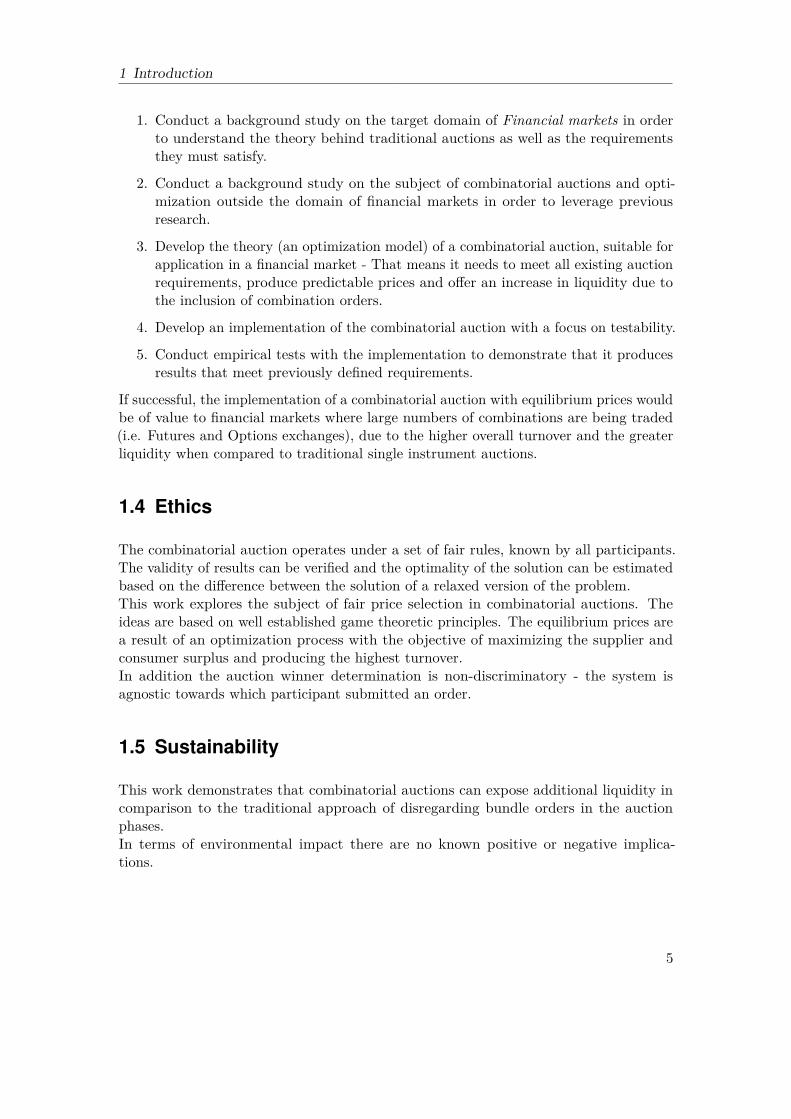
1. Conduct a background study on the target domain of Financial markets in orderto understand the theory behind traditional auctions as well as the requirementsthey must satisfy.

2. Conduct a background study on the subject of combinatorial auctions and opti-mization outside the domain of financial markets in order to leverage previousresearch.

3. Develop the theory (an optimization model) of a combinatorial auction, suitable forapplication in a financial market - That means it needs to meet all existing auctionrequirements, produce predictable prices and offer an increase in liquidity due tothe inclusion of combination orders.

4. Develop an implementation of the combinatorial auction with a focus on testability.

5. Conduct empirical tests with the implementation to demonstrate that it producesresults that meet previously defined requirements.

If successful, the implementation of a combinatorial auction with equilibrium prices wouldbe of value to financial markets where large numbers of combinations are being traded(i.e. Futures and Options exchanges), due to the higher overall turnover and the greaterliquidity when compared to traditional single instrument auctions.

1.4 Ethics

The combinatorial auction operates under a set of fair rules, known by all participants.The validity of results can be verified and the optimality of the solution can be estimatedbased on the difference between the solution of a relaxed version of the problem.This work explores the subject of fair price selection in combinatorial auctions. Theideas are based on well established game theoretic principles. The equilibrium prices area result of an optimization process with the objective of maximizing the supplier andconsumer surplus and producing the highest turnover.In addition the auction winner determination is non-discriminatory - the system isagnostic towards which participant submitted an order.

1.5 Sustainability

This work demonstrates that combinatorial auctions can expose additional liquidity incomparison to the traditional approach of disregarding bundle orders in the auctionphases.In terms of environmental impact there are no known positive or negative implica-tions.

5

1 Introduction

1.6 Methods

The work combines qualitative research for collecting of requirements and the develop-ment of a theoretical model with quantitative research for the system development andtesting. The selection of specific methods is based on The portal of research methods andmethodologies[11].The philosophical assumption for this project is positivism since results produced by thedeveloped system are objective and measurable and independent of the observer[11].The research methods used are Conceptual[11] for the theory development componentand Applied[11] in the system development portion of the work.The research approach employed is Inductive[11] as through the course of the development,different theories were tested before arriving at an optimal solution.The research methodologies chosen are Experimental[11] as there is the ability to con-duct fully controlled experiments and adjusting specific input parameters for test casesperformed.The data collected is the result of experiments, thus method used is Experiments[11]For data analysis the project utilizes Statistics[11] as a research method as values wereused to demonstrate the quality of produced solutions as well as the tractability of inputs.Quality assurance - test results presented can be replicated and are not ambiguous intheir interpretation, that is key figures measured such as price values, runtime and IP/LPgap.

1.7 Delimitations

With discrete optimization small changes to the input can often have a drastic impact onthe computation time. It would be useful to test all combinations of "low - mid - high"gradients for the 9 parameters defined for each test case in order to identify which setups at most difficult. Unfortunately, the would result in 39 individual tests and it fallsoutside the scope of this project.

Development of an advanced user interface for the software is not the focus of this workand therefore also falls outside the scope of the project.

1.8 Outline

Chapter 2Provided is introductory information for financial markets and auctions. Both subjectsare broad and covering all aspects is outside the scope of this project. Instead, supplied isinformation that directly applies to combinatorial auctions. Introduced are the exchangesand their purpose, order matching, equilibrium prices, the use of auctions in financialmarkets, and auction types.

6

1 Introduction

Chapter 3The Combinatorial Auction problem in this report is modeled as an Integer Program.This chapter introduces basic concepts used later in the report. Since the subject hasbeen extensively studied, it is out of the scope of this project to provide an extensiveoverview on Integer programming. Therefore, the only covered aspects are: problemmodeling, basics on how models are solved and a brief overview on available systemshandling integer programs.

Chapter 4Presented is the core contribution of the thesis work. Provided is a formalization of require-ments, a combinatorial bidding language and a description of the integer programmingmodels. The overview is supplemented with examples.

Chapter 5Provided are test results and analysis of the models described in Chapter 4. Test casesare well defined and structured in a way that illustrates the correctness and tractabilityof the model with different input sizes. Two types of tests were involved - synthetic testsand test with real order data.

Chapter 6The chapter presents a conclusion of the research and suggests a direction for future workon the subject.

7

2. Auctions in Financial Markets

In everyday language the term auction is often associated with a sale of a good to thehighest bidder. However, the subject is far broader as there are many different types ofauctions.

More abstractly, an auction is a set of rules facilitating the trade of goods or services.Further in this chapter presented are auction properties based on which a categorization isintroduced with the aim of providing an overview of different types of auctions. Follows anintroduction to the concept of equilibrium prices and a description of the specific auctionscommonly used in financial markets today. The chapter concludes with a discussion onthe need for combinatorial trading.

2.1 Auction classification

The following is an incomplete list of auction properties which is information from [9]and [8].

1. Dimensionality refers to what is used in the valuation of an asset. For instance inan antiques auction the price of a product would be determined by multiple factors:quality, condition, rarity etc. Such auctions are multi-dimensional as there aremultiple components influencing the price. An auction is single dimensional whenthe goods traded are fungible and there is one aspect to influencing the valuation.

2. Auctions can be single sided or double sided. In the case when there is one buyeror seller and multiple participants competing to trade, the auction is single sided.For instance several buyers could be competing with each other to obtain a goodat the lowest possible price from a supplier. Another example are procurementauctions, also known as reverse auctions where there are there are multiple supplierscompeting for a contract with one consumer. On the other hand, dual sidedauctions, traditionally also known as exchanges, allow multiple buyers and sellersto be matched together.

3. An auction can be Open outcry in which case all bids are publicly known to thecompeting participants. This allows each participant to adjust their bid based on

2 Auctions in Financial Markets

competitor information. The alternative is the Sealed bid format where orders areprivate, shared with the "auctioneer" but not with competing parties.

4. A single unit auction deals with unique assets/contracts i.e. the quantity is equalto one. In auctions where assets are fungible there can be supply or demand formore than one unit - such auctions are known as multi-unit.

5. There are different rules for establishing the trade prices in an auction, depending onthe specific requirements and also the number of sides. With single-side single-unitauctions pricing is easier - there are the first-price and kth-price strategies. In afirst-price auction, the highest bidder is selected as a winner and the trade price istheir bid price. This is the typical method used by auctions. A kth-price auctionalso selects the highest bidder but they pay the price of the kth-best order (k couldbe the second or third bid). This strategy is useful in sealed bid auctions as itprevents participants from misrepresenting their true valuation of the asset.Selecting the trade price in double-sided multi-unit auctions is less trivial. This isdone by establishing an equilibrium price tick at which the marked is uncrossed- orders that accept the price are traded and orders more generous than theequilibrium price are guaranteed to be traded in full. This concept is covered inmore depth in this chapter.

6. Typically orders specify a buy or sell operation for one specific tradable instrument.This means individual auctions are created on per-instrument basis. Such auctionsare classified as single-item (single-instrument). When orders specify a combinationof multiple instruments, a different type of auction must be used, known as multi-item or simply a combinatorial auction. In this case instruments are contingentupon each other and therefore they must be considered simultaneously.

For illustrative purposes the auction categorization is shown below in Figure 2.1. Withthe presented classification, the combinatorial auction required for a financial marketplacecan more accurately defined as "Single-dimensional, Sealed bid, Dual-sided, Multi-unit,Combinatorial (Multi-item), Equilibrium price".

9


Auction

Multi dimension

......

Single dimension

Open outcry

......

Sealed bid

Single sided

......

Dual sided

Single unit

......

Multi unit

Single item

First price k-th price

Combinatorial

Equilibrium price

Figure 2.1: Auction categorization

2.2 The Equilibrium price

In economics the concept of equilibrium price is well understood and accepted as theonly stable price given a free market[12]. That is the level at which supply meets demandwithout free disposal or where the supply and demand curves intersect[1].Auctions used on financial markets implement this principle, thus providing a fair anaccurate representation of the market for a given time period.

in order to illustrate the ideas defined are the bid and ask quantities as follows:

• Bid quantity for a price - the sum of the quantities of all bid orders that accept aprice.

• Ask quantity for a price - the sum of the quantities of all ask orders that accept aprice.

Consider the following example:

For the arbitrary good A the demand is as follows:At price $21 the aggregate quantity demanded is 105 units.At price $22 - 70 units.At price $23 - 40 units.At pride $24 - 15 units.The aggregate supply for A is as follows:At price $21 supplied are 5 units.At price $22 - 15 units.

10


At price $23 - 40 units.At price $24 - 80 units.

The supply and demand curves of the example are plotted in Figure 2.2. Naturally, thelower the price the greater the quantity demanded is, while the quantity supplied isgreater with increasing the price. From Figure 2.2 it is evident that the equilibrium priceis $23, at the intersection of the curves.

21 22 23 245

15

40

7080

105

Price ($)

Qua

ntity

Supply and demand accepting the prices

DemandSupply

Figure 2.2: Supply and demand curves with equilibrium price 23$.

Each curve point represents quantity across all orders that accepts the price. It isimportant to note that in practice, not any real value on the piecewise curve is a validprice.The smallest price increments allowed are known as price ticks. In this example weassume a price tick of $1 for simplicity but regardless of the tick sizes, prices levelsare discrete values. As a result, often the intersection of supply and demand is notat a discrete price. If we consider another example where the the supply and demandquantities are as expressed in Table 2.1, the intersection happens to be between priceticks $22 and $23 (Figure 2.3).

Price Bid quantity (Demand) Ask quantity(Supply)21 120 1022 75 3023 40 6024 15 100

Table 2.1: Supply and demand quantity 1.

11


21 22 23 2410153040

6075

100

120

Price ($)

Qua

ntity

Supply and demand accepting the prices

DemandSupply

Figure 2.3: The intersection of supply and demand is between prices 22$ and 23$.

It is evident that since price ticks can only be discrete values, piecewise curves are lessmeaningful. Using stepwise graphs instead reveals more information. First, defined arethe terms auction turnover and imbalance as follows:

• Turnover - the smallest of the bid or ask quantities at a price tick. This representsthe quantity that can trade at this price.

• Imbalance - the bid quantity subtracted by the ask quantity.

The example from table 2.1 can be extended to include the turnover and imbalance valuesfor each price tick (Table 2.2):

Px Bid Ask T/O Imb21 120 10 10 11022 75 30 30 4523 40 60 40 -2024 15 100 15 -85

Table 2.2: Uncross table 1.

The supply and demand quantities are plotted as stepwise curves with discrete prices onthe x axis and the quantity on the y axis as show in in Figure 2.4. This representationshows that the intersection of supply and demand is at price tick $23 which is also theprice tick that has the highest turnover as shown in Table 2.2.

12


20 21 22 23 24 2510153040

6075

100

120

Price ($)

Qua

ntity

DemandSupply

Imbalance

Figure 2.4: The blue area represents the quantity at a price accepted by buy orders. The red area is thequantity accepted by sell orders. The imbalance for a price tick is the demand - supply delta.

There are cases in which there are more than one price levels that result in the samehighest turnover value. This problem can be solved in several ways but the most fairapproach is by considering the imbalance as well. Follows a complete set of rule for priceselection in the possible scenarios[13].

1. If there is one price achieving maximum turnover, that price is selected.

2. If multiple price ticks achieve the same maximum turnover, the price tick with thehighest turnover and lowest absolute imbalance is selected. If there are severalprice ticks with the same maximum turnover and minimum imbalances, additionalrules (2a, 2b, 2c and 2d) apply[13]:

a) If all prices in the interval have positive imbalance, selected is the highestprice in the interval[13].

b) If all prices in the interval have negative imbalance, selected is the lowest pricein the interval[13].

c) If all prices in the interval have zero imbalance, selected is the midpoint ofthe interval. (If the midpoint is between two price ticks, selected is the pricethat represents an even number of ticks)[13].

d) If the absolute imbalance is equal in the interval, but some prices have positiveimbalance and some prices have negative imbalance, identified are the twoadjacent prices that have different signs. Of these two prices, selected is theprice that represents an even number of ticks[13].

The aim of sub-rules 2a and 2b, for the case of multiple price ticks with the same highestturnover is to guarantee that orders more generous than the selected price will be tradedcompletely. For buy orders more generous means higher limit price or "willing to pay

13


more" while for sell orders that is lower limit price, or "willing to sell for less".The purpose of sub-rules 2c and 2d is simply for handling the described ambiguities thatcould occur.Rules 2a, 2b, 2c and 2d are supplemented with examples in Appendix A.

2.3 Single-item auction problem formulation

In this section presented is a formal interpretation of the single-item auctions used byfinancial markets today. The following common requirements were gathered throughanalyzing auction specifications of exchanges[2][14][15][16]:

• The market price selected is optimal - the auction turnover is maximized. Whenthere are more than one price ticks with the same maximum welfare, the price withthe smallest difference between quantity demanded and quantity supplied knownas imbalance.

• The price is non-discriminatory. The only parameters used in price determinationare the quantities of the supply and demand, i.e. there is no regard for the identitiesof participants.

• Achieved is incentive compatibility. Participants receive no additional utility frommisrepresenting their truthful valuation for an instrument. In Game Theoreticterms that means that the best strategy of a participants is to submit an orderwith their truthful valuation.

• Buy and sell orders are uncrossed (Non-trade through rule). All supplied orrequested quantity more generous than the selected price tick are matched. Forthat reason the price is also referred to as uncross or "market clearing".[17]

In order to formalize the requirements the following definitions are introduced:Bid orders for a particular instrument are notated as bj

i and Ask(sell) orders are notatedas aj

i . All orders have price and quantity attributes - i.e. bji .price, a

ji .price and bj

i .qty,aj

i .qty. Based on order valuations constructed are the price ticks in Orderbook i. A pricetick for i is notated as pi.

Defined are the terms "at the money" and "in the money". An order is "at the money" inrelation to a price tick if the order’s limit (reserve) price is exactly the same as the pricetick. An order is "in the money" in relation to a price tick if the order’s limit price ismore generous than the price tick[13]. Buy orders are more generous when their price isgreater than a price they are compared to and sell orders are more generous when theirprice is lower than the price they are compared to.The above can be summarized as follows:

• Aat - aggregate supply quantity "at the money" which can be traded.

• Ain - aggregate supply quantity "in the money" which must be traded.

14


• Bat - aggregate demand quantity "at the money" which can be traded.

• Bin - aggregate demand quantity "in the money" which must be traded.

Any quantity that is "in the money" must be traded because of the strict "non-tradethrough" rule - at a given price any orders that are more generous must be tradedcompletely.The auction turnover T for price tick pi is defined as:

T (pi) = min(Aati +Ain

i , Bati +Bin

i ) (2.1)

The auction imbalance I for price tick pi is defined as:

I(pi) = Bat +Bin −Aat −Ain (2.2)

As per the rules defined in section 2.4 we maximize the turnover T first and use theimbalance I only if there are multiple solutions (price ticks) with the same maximumvalue. The turnover in (2.1) is defined as the lower of the bid quantity that accepts theprice or the ask quantity that accepts the price as this is the amount that will trade.The imbalance (2.2) is defined as the difference between the bid quantity accepting theprice and the ask quantity accepting the price.Additionally the following restrictions are imposed:

Aini ≤ Bat

i +Bini (2.3)

Bini ≤ Aat

i +Aini (2.4)

Constraints (2.3) and (2.4) enforce that the selected price tick is such that the market isuncrossed and any supply or demand quantity more generous than the price is tradedcompletely[13]. The pricing rules expressed verbally in section 2.2 and illustratedthrough the examples in Appendix A satisfy constraints (2.3) and (2.4), proven in[13].

The auction problem is in finding the price tick pi where the turnover T (pi) is maximizedand the orders are uncrossed. Once the optimal price is selected, allocation is trivial -orders that are "in the money" are given priority over orders "at the money". Orders at themoney are filled in FIFO or pro-rata fashion (First-in, First-out)[13].

2.4 Combination orders

There are cases when it is beneficial for a broker to trade an instrument if and only ifthey also succeed in trading another instrument. That means the possibility of arrivingat an in-between position where only some of the instruments are traded is undesirable

15


and presents a risk[18], known as the exposure problem[4].A combination (bundle) order specifies participation quantities for the instrumentsinvolved, number of combinations requested (order quantity) and a limit price for thebundle. The instruments requested by a combinatorial orders are also known as legs oratoms.Consider pseudo order i in the following example:

Order iInstrument A1: ’buy x1’Instrument A2: ’buy x1’

Bundle price: $8Bundle quantity: 2

Order i specifies that it is atomically buying 1 of each instrument (A1 and A2) and iswilling to pay up to $8. The bundle quantity of 2 indicates that two such bundles arebought. With the information of order i it can be concluded that the broker submittingit is interested in obtaining instruments A1 and A2 in pairs[19].

Notable use cases of combinatorial auctions include the selling of the radio frequenciesspectrum since for buyers it is beneficial to obtain neighboring ranges; auctioning ofairport take-off and landing time slots as well as the servicing rights for bus lines in largemetropolitan areas[4].Within the domain of financial markets, combinatorial orders allow participants to expressinflexible or very specific supply or demand preferences. For instance, an investmentbank may deem beneficial to adjust their portfolio in a very specific way and if notpossible, not make a change. In this case a combination order lowers the risk for thetrader.

A prime example of combinatorial trading in security exchanges are orders known astime spreads[20]. Such combinations have a sell operation for one future contract and abuy operation for another contract on the same underlying instrument. The contract soldmay be with delivery date x and the contract bought with delivery date x+ 1 month.Depending on market prices and interest rates the price value of a time spread may bewith a positive or negative sign or equal 0 when the contract prices is the same.Timespread orders can be used for practical reasons due to a changes in demand or by investors,speculating on the slope of the price curve[20].

Many exchanges allow for combinations to be traded during continuous trading with theuse of bait orders (also know as derived orders)[21], however, at the time of writing thisreport, the author is not aware of financial markets that include combination orders intheir auction phases. Some next day spot electricity markets use combinatorial auctionsin the computation of their base prices for each hour of the day[22].Unlike the traditional single-item auctions, combinatorial auctions (CAs) have to definetwo sets of constraints - for asset/instrument participation and price restrictions. This isbecause bundles cannot trade partially.

16


2.5 Previous and related work

Much of the previous work on Combinatorial auctions[8] focuses only on the optimalwinner selection part of the problem [24][28]. However, in order to be useful in the contextof a financial marketplace, the combinatorial auction needs to produce equilibrium pricesfor all instruments involved in the combination legs.

The work of Xia, Mu and Koehler, Gary J. and Whinston, Andrew B. - Pricing combina-torial auctions explores two methods of pricing of dual sided combinatorial auctions: theDeMartini pricing[29] method and the O’Neill pricing[30]. Both methods however relyon two steps. Firstly, a winner selection is made with an optimization model and second,based on the winner selection, instrument prices are constructed based on valuations ofthe winners. This approach however is not sufficient to guarantee that the best allocationwas made. This is because if the price vector was known prior to the optimization, theremay have been a better set of winners. It is required to consider prices and instrumentparticipation restrictions simultaneously.

The publication Computationally Manageable Combinational Auctions by Rothkopf,Michael H. and Pekeč, Aleksandar and Harstad, Ronald M.[4] discusses the relevanceand necessity of combinatorial auctions, introducing the "threshold" problem and risk ofnon-combinatorial bidding. Presented is a mathematical model for the generic winnerdetermination of a single-sided (multiple buyers, single supplier), single-unit auctionswhere it is demonstrated that restricting the types of bid combinations significantlyimproves tractability[4]. Specialized algorithms dealing with single sided auctions havealso been created[23].

Further work by Sandholm, Tuomas Winner determination in combinatorial auction gener-alizations [25] examines a dual-sided auction with and without free disposal - i.e. multiplebuyers being matched with multiple sellers and the selection have to be made so that sup-plied quantity matches exactly the demanded quantity. Their empirical test results suggestthat allowing free disposal significantly reduces the complexity.

A paper by Andersson, A. and Tenhunen, M. and Ygge, F. Integer programming forcombinatorial auction winner determination[26] presents an several algorithms and aninteger programming model for the single-sided, multi-unit auction with empirical testresults demonstrating the impact of the input probability distributions on the tractabilityof the problem.

The work of Kothari, Anshul and Sandholm, Tuomas and Suri, Subhash Solving Com-binatorial Exchanges: Optimality via a Few Partial Bids[27] demonstrates achievingmaximum surplus (auction optimality) by allowing some allocated orders to be partiallyfilled.

Not all auctions discussed in [4], [25] and [26] fully satisfy the auction requirements in thecontext of a financial marketplace due to the fact that the models do not achieve theiroptimal result at an equilibrium price vector. However ideas for relaxing the problem vie

17


either partial filling of some orders or allowing free disposal were used in developing thehybrid auction model presented in chapter 5.

The issue of pricing, omitted in [4], [25] and [26] is discussed in the paper of Xia, Mu andKoehler, Gary J. and Whinston, Andrew B. Pricing combinatorial auctions [31]. Discussedis the problem of incentive compatibility for combinatorial auctions - the exact issue thatstandard non-combinatorial auctions solve in financial marketplaces. The work explorestwo methods for obtaining the equilibrium prices per-instrument - the "DeMartini"[29]and the "O’Niel"[30] pricing methods. However, the method employed is two step - Firstlythe best winner selection is made, from which market prices are subsequently inferred.That approach doesn’t guarantee that if a different price vector was selected there wouldnot exist a better winner selection. Therefore it is required that price selection is donebefore or in the same step as winner determination.

The work of Schellhorn, Henry Combination trading with limit orders [18] models a dualsided equilibrium priced combinatorial auction with a fixed point algorithm which uses ap-proximated aggregate demand/supply functions for price determination.

Auctions used withing financial markets ensure that trading occurs at the same (equilib-rium price). This is a very important property because of:

• The price is a true reflection of the market.

• Predictability - Once a price is established it is obvious to participants why theirorder traded or didn’t trade.

Since a combinatorial auction has to consider all contingent instruments simultaneously, itneeds to discover the optimal price vector and the best allocation at the same time. Wileprevious work shows that in the general case the combinatorial auction problem is NP-hard,in the context of financial markets there is an important consideration - there is typicallya mix of combination and single orders which has the possibility of relaxing the problem.This exact characteristic of the inputs is exploited by this work, while adding the additionalconstraint of choosing prices and allocations simultaneously.

18

3. Integer Programming

Integer programming[32][33] is a special case of mathematical programming[34]. In thiscontext the term "programming" is different from "computer programming" as it is moreclosely related to "planning"[34].

An optimization model is a problem of the type:max{f(x) : x ∈ X, g(x) ≤ 0} where x ∈ X, g(x) ≤ 0, the restrictions for variable xare known as constraints and f(x) is the objective function [35]. A common featureof mathematical models is the involvement of optimization, meaning we maximize orminimize a value[34].

Mathematical programming can be classified as[33]:

• Linear Programming (LP)

• Non-Linear Programming (NLP)

• Integer Programming (IP)

The auction problems subject of this report involve optimization - required is a pricetick and allocation producing the highest the social welfare, subject to specific auctionconstraints[9][8]. Both the objective function and the constraints can be expressed aslinear relationships. Integer programs are a special case in linear programming where thevariables assume only discrete (integer) values. Solving models with integer variables isalso known as discrete optimization.

Integer programming (IP)[33] problems can be classified as follows:

• Pure integer programming (PIP)[36] - All variables are discrete values

• Mixed integer programming problem (MIP)[36] - Some variables are discrete valuesand others are allowed to be real numbers

• Binary (mixed) integer programming[36] - Integer variables are restricted to 0 or 1.

3 Integer Programming

The use of integer constraints is required when the variables represent discrete units(e.g. cars, houses) or when the variable represents a "yes/no" type of decision[36]. Inthe combinatorial auction problem variables represent the order allocation - whetheror not an order has been selected as winning or not, which warrants the use integervariables.

The subject of integer optimization has been extensively researched, therefore this chapterserves to only introduce the basic concepts used in modeling and solving the combinatorialauction.

3.1 Problem Modeling

In order to create a mathematical model of a problem, the following is required:

• Establish the input parameters and the variables

• Construct a maximization or minimization objective function

• Construct the constraints imposing restrictions meaningful for our problem

3.1.1 LP: The Product Mix problem

To illustrate problem modeling in practical terms presented is the example of the "ProductMix" problem described in[37]:

A steel mill can produce two products - Product P1 and Product P2.The mill can produce 200 tons of P1 per hour which yields a profit of 25$ per ton. Thedemand for P1 is 6000 tons. The mill has to produce at least 1000 tons of P1.Product P2 is produced at rate of 140 tons per hour but the profit is 30$ per ton. Thedemand for P2 is 4000 tons. The mill has to produce at least 2000 tons of P2.The available production time is 40 hours. The goal is to design a production plan thatmaximizes the mill’s profit.

In order to model the problem from the above example introduced are two vari-ables:

x1 = Tons of product P1x2 = Tons of product P2

The profit per ton for P1 is 25$ and for P2 is 30$, therefore our objective functionis:

Maximize : 25x1 + 30x2

20


Formulated is the constraint for the available production time of 40 hours:

Subject to : 1200x1 + 1

140x2 ≤ 40

In addition created are the two constraints for the minimum and maximum of P1 and P2that can be produced:

1000 ≤ x1 ≤ 6000 (3.1)2000 ≤ x2 ≤ 4000 (3.2)

The constructed linear programming model can be solved using the simplex methodwhich is implemented by most linear programming solvers.The result is as follows:Objective value (profit) = 188571.4286x1 = 5142.86, x2 = 2000

There are specialized languages for algebraic modeling at a high level such as AMPL (AMathematical Programming Language)[38]. In the AMPL format, parameters, variablesand constraints are expressed with syntax very similar to the mathematical notation. Asa practical consideration, it is significantly easier to implement models in the AMPLformat.

To illustrate the AMPL syntax, the model for the "Product mix" problem from figure 3.2looks as follows:

var x1 >=1000, <= 6000;var x2 >=2000, <= 4000;maximize profit: 25*x1 + 30*x2;subject to time: (1/200)*x1 + (1/140)*x2 <= 40;

3.1.2 IP: The knapsack problem

Creating an Integer programming (IP) model is similar to developing an LP model withthe addition of constraints enforcing that variables can only be integers. However, it isimportant to note the profound difference in the solution that can create.This is illustrated in the example from Model Building in Mathematical programming byH. Paul Williams, chapter 8.2.2, page 156[34]:

Maximize : x1 + x2 (3.3)Subject to : −2x1 + 2x2 ≥ 1 (3.4)

−8x1 + 10x2 ≤ 13 (3.5)x1, x2 ≥ 0 (3.6)

(3.7)

21


If variables x1 and x2 (3.6) from the above example: Example 2 represent the quantityof indivisible goods such as cars or airplanes, they should be integer values. However,there is no need for such restriction if x1 and x2 represent gallons of a liquid.

The optimal solution of the described LP is achieved with values:

x1 = 4 and x2 = 4.5.

On the other hand, if we restricted the variables to be discrete values, the optimal solutionis achieved with:

x1 = 1 and x2 = 2.

Simply rounding down the LP solution gives values that are infeasible as per the constraintdefined in (3.4), (3.5) and (3.6).

Discrete optimization is illustrated with the well known knapsack problem[36]:

Given are a set of objects, each with a weight and value. There is a knapsack with aspecified weight capacity. The objective is to place items in the knapsack in such a waythat its capacity is not exceeded and the total value collected is maximized.Object 1: value 8, weight 5Object 2: value 11, weight 7Object 3: value 6, weight 4Object 4: value 4, weight 3Knapsack capacity: 14

Introduced are four binary allocation variables: x1, x2, x3 and x4, each corresponding tothe selection decision for objects 1, 2, 3 and 4.

This allows us to express the knapsack problem as follows:

Maximize : 8x1 + 11x2 + 6x3 + 4x4 (3.8)Subject to : 5x1 + 7x2 + 4x3 + 3x4 ≤ 14 (3.9)

xi ∈ {0, 1} (3.10)

In order to generalize this model the number of objects is denoted with n so that theset of all object is {1, .., n}. The weight of object i is expressed with the parameter wi

and the value of object i is expressed with parameter vi where i ∈ {1, .., n}. Variable xi

22


is the selection (allocation) variable for object i. The knapsack capacity parameter isdenoted with C. The problem becomes:

Maximize :n∑

i=1vixi (3.11)

Subject to :n∑

i=1wi ≤ C (3.12)

xi ∈ {0, 1} (3.13)

If the selection of fractions of objects was allowed, i.e. without constraint (3.13), thesolution would be a selection of the highest value per weight unit first followed by fillingremaining capacity with the next best object. In the above knapsack formulation in itsLP form (without (3.13)) the resulting selection would be:

x1 = 1, x2 = 1, x3 = 0.5 and x4 = 0

3.1.3 Logical conditions

When implementing a problem into a mathematical model it is often required to han-dle logical conditions of the type "If condition is true, apply constraint X". In con-trast to computer programming, expressing conditions can be difficult in optimizationmodels[34].

Consider the knapsack problem. Suppose that Objects 2 and Object 3 are a pair and if oneis selected the other must be selected as well. Since the allocation variables for objects 2and 3 are x2 and x3 respectively, the constraint can be expressed as:

Subject to : x2 − x3 = 0

That constraint is met only when Object 2 and Object 3 are both selected or none of thetwo are selected.

3.1.4 The Big M Method

Some logical conditions with multiple variables are difficult to express as a linear inequality.A known workaround involves introducing a large positive penalty constant[34].For instance suppose we have two variables y ∈ N and x ∈ 0, 1. Suppose that it isrequired to express the constraint that y ≤ 10 if and only if when x = 1.In integer programming this can be achieved with a variation of "The Big M Method".The constraint is as follows:

23


y ≤ 10 +M(1− x)

Where M is a large positive constant, greater than any value y can assume. This methodis used in the combinatorial auction formulation in Chapter 5.

3.2 Problem Solving

Linear programming models are solved using variations of George Dantzig’s simplexalgorithm[33] which is implemented in modern LP solvers. Discussing the simplexalgorithm is out of the scope of this project. Further information on the simplex methodis available at [33].

Integer optimization is performed by solving the LP problem multiple times in a branch-and-bound fashion. When a non-discrete value is encountered, the system creates twonew LP problems with additional constraints. In the first new LP the branch variable isset to the round-up value and in the second to the round-down value.For that reason, IP problems are many times more computationally complex than anequivalent linear program. An integer program with its integer constraints removed isknown as the "Linear relaxation" (LR)[34][33] of the model.

Since the Linear relaxation (LR)[33] is less constrained than the integer program (IP)[33]the following rules are inferred[36]:

1. If the (IP) is a minimization, the optimal objective value of the (LR) is less thanor equal to the optimal objective value for (IP)

2. If the (IP) is a maximization, the optimal objective value for the (LR) is greaterthan or equal to the (IP)

3. If the (LR) is infeasible, then (IP) is infeasible too.

4. If (LR) is optimal with integer variables, then this is the best (IP) solution.

5. If the coefficients in the objective function are integer, then for minimization, theoptimal objective for (IP) is greater than or equal to the "round up" of the optimalobjective for (LR). For maximization, the optimal objective for (IP) is less than orequal to the "round down" of the optimal objective for (LR).

Therefore, solving the Linear relaxation fist gives boundaries for the IP solutions. Thedifference between the objective value of an integer solution and that of the linearrelaxation is known as the IP/LP gap.

24


3.2.1 Branch and bound

The basic principle for discrete optimization used by solver is know as branch-and boundsearch. The fundamentals of the concept are illustrated using the knapsack exampleproblem.

Maximize : x1 + x2 (3.14)Subject to : −2x1 + 2x2 ≥ 1 (3.15)

−8x1 + 10x2 ≤ 13 (3.16)x1, x2 ≥ 0 (3.17)

(3.18)

The solver performs the following steps:

1. Solve the (LR) linear relaxation[33].The solution is x1 = 1, x2 = 1, x3 = 0.5, x4 = 0 with objective value of 22.The solver now knows that no integer solution can have objective greater than 22.

2. Branch on variable x3.Since the value for x3 is not an integer, the solver performs branching ? two newlinear problems are created. In the first one, it enforces x3 = 0 and in the secondproblem it enforces that x3 = 1.Solving the (LR) of the resulting two nodes give us the solutions:Node x3 = 0: Objective = 21.65, x1 = 1, x2 = 1, x3 = 0, x4 = 0.667Node x3 = 1: Objective = 21.85, x1 = 1, x2 = 0.714, x4 = 0The solver now knows that the IP solution is no greater than 21.85. In fact sinceobjective value has to be an integer, the solver knows that the objective of the bestinteger solution can be no greater than 21.

3. Branch in the x3 = 1 node on variable x2 where the value was 0.714. For theresulting two new (IP) where we enforce x2 to be 0 or 1 we get the followingsolutions:Node x3 = 1, x2 = 0: Objective = 18, x1 = 1, x2 = 0, x3 = 1, x4 = 1Node x3 = 1, x2 = 1: Objective = 21.8, x1 = 0.6, x2 = 1, x3 = 1, x4 = 0The solver now has a feasible integer solution with objective = 18. When an integersolution is reached there is no further branching from that node. So far this is thecurrent best solution.

4. Branch in the x3 = 1, x2 = 1 node on variable x1 where the value was 0.6. Forthe resulting two new (IP) where we enforce x1 to be 0 or 1 we get the followingsolutions:Node x3 = 1, x2 = 1, x1 = 0: Objective = 21, x1 = 0, x2 = 1, x3 = 1, x4 = 1Node x3 = 1, x2 = 1, x1 = 1: InfeasibleThe best integer solution is with objective 21.

25


5. The node with x3 = 0 where the objective was 21.65 is still unexplored but fromsolving the (LR) the solver knows there are no better solutions. The searchterminates.

The search process is drawn in Figure 3.1.

Objective 22x1=1 x2=1 x3=0.5 x4=0

Objective 21.65x1=1 x2=1 x3=0 x4=0.667

Objective 21.85x1=1 x2=0.714 x3=1 x4=0

Objective 18x1=1 x2=0 x3=1 x4=1

Objective 21.8x1=0.6 x2=1 x3=1 x4=0

Objective 21x1=0 x2=1 x3=1 x4=1

Infeasible

Figure 3.1: Branching on non-integer variables until we reach an integer solution. If the solution is notguaranteed to be the best possible one, the algorithm backtracks and branches on anothernon-integer variable from the preceding node.

In addition to branch and bound, optimization software can utilize various heuris-tics for reducing the size of the search tree, for instance there is a variation of thebranch and bound algorithm involving cutting planes. For further information refer to[34].

26

4. The Equilibrium Price Combinatorial Auction

The development of an efficient implementation of the combinatorial auction problemis done in an iterative fashion. In this chapter introduced are three formulations of theauction using integer programming techniques.

• Model 1: Brute force - This approach is heavily inspired by previous work onthe subject and constitutes of selecting a range of price vectors to be tested. Anoptimization problem is then solved for each price vector in the range.

• Model 2: Priced WDP - The optimization problem is solved once with additionalvariables and constraints for the prices.

• Model 3: Priced hybrid WDP - This approach combines the curve point winnerdetermination in single instrument auctions with the priced combinatorial WDPfrom Model 2. Model 3 is useful when a large portion of the orders are singleinstrument.

The auction models were implemented in the AMPL format. That means that the solverreceives the following inputs:

• The AMPL model containing constraint and objective definitions along with vari-ables and parameters.

• The AMPL data containing the parameter values.

• Solver configuration.

It is required to introduce an order notation that can easily be synthesized as AMPL datafiles. In order to facilitate testing of the models, an application that performs synthesisof AMPL data files is developed.Testing is performed in two ways - with the use of generated orders with predictableinstrument prices and with the use of real market data.

4 The Equilibrium Price Combinatorial Auction

4.1 System overview

The test system is composed of:

• Input data generation components.

• Input (Model, Data, Configuration).

• Optimization component (Third party software).

• Output (Subject to analysis).

Figure 4.1 illustrates at a high level the system components facilitating testing of theauction models developed. The input orders (AMPL Data) are formated specifically tothe model under test, therefore a highly modular design was chosen.

28


Synthetic Orders Real Market Data Orders

Optimizer input

Optimizer output

Data synthesisOrder generator

Generationconfiguration

Log parser

System logs

Optimizer(CPLEX / GLPK)

AMPL ModelOptimizer

configuration

AllocationPrice vector

Orders Orders

AMPL Data

Figure 4.1: System overview

4.1.1 Input data synthesis

Test scenarios are either generated from a configuration file or based on order data providedby an exchange. Synthetic orders are generated based on configuration specifying theproperties of the input including single/combinatorial orders ratio, mean instrumentvaluations and buy/sell price crossing.

In the case of tests with real order data, orders are read from a logs file and parsed into thesame format output produced by the synthetic order generator. Shown below are three

29


example orders that can be input for the data synthesis component. Inside the braces arethe bundle leg ratios, followed by the price and number of bundles.

{0,0,1,0,0,0,0,0,0,0,1,1};588;1{1,1,0,0,-1,0,0,0,0,0,0,1};323;1{0,1,1,0,0,0,0,1,0,-1,1,0};477;1

Format: {leq_1_quantity, ..., leg_12_quantity}; price; bundle_quantity

4.2 Requirements

Defined are the following auction requirements which are implemented in the modelsdescribed in section 4.4:

1. The quantity traded for an order can be no greater than the quantity specified byan order.

2. An order can be traded (filled) partially as long as it is not of an "all-or-none" type.

3. Orders that are "all-or-none" must trade their quantity in full or not at all.

4. No market participant benefits from misrepresenting their valuation, i.e. the beststrategy of every trader is to submit a bid or ask with their true valuation.

5. The allocation of orders in the auction is based on calculated equilibrium prices forall instruments.

6. The equilibrium prices for all instruments (or price vector) are selected in a non-discriminative fashion - i.e. the price is the same for every market participant.

7. Single instrument orders are not traded through (more generous orders are givenpriority and always traded in full).

8. Combination orders are allowed to trade through because constraining them tonon-trade through reduces auction turnover significantly.

9. The price vector is selected such the highest possible auction turnover is achieved.

10. The winner selection of combination orders is such that the highest possible auctionturnover is achieved.

11. Orders specify a limit price beyond which no matching can occur. Single instrumentbuy orders selected must be with a limit price greater than or equal to the selectedequilibrium price for the instrument. Single instrument sell orders must be with alimit price less than or equal to the equilibrium.

12. Combinatorial auctions are priced based on the net bundle valuation. The meansnegative prices are valid, as well as a price of 0.

30


13. A trade price of a bundle can be calculated using the selected instrument prices. Acombinatorial order can be matched only if the calculated trade price is less thanor equal to the limit bundle priced submitted by the order.

14. The equilibrium price vector is selected to be such that orderbooks are uncrossedwith respect to the non-restricted single instrument orders. That mean at theselected price for each instrument, all orders more generous than the equilibriumprice are traded in full.

All of the above requirements are implemented in the three optimization models de-veloped and are part of the quality assurance process (requirements are never vio-lated).

4.3 Model formulation

Given an input of combinatorial orders on a set of instruments, the winner determinationproblem (WDP) is finding the optimal set of winning (allocated) orders such that theauction turnover is maximized. A requirement, common for financial markets, is that themaximized turnover is achieved at equilibrium uncross prices for all instruments traded.The auction has to output bundle order allocation values and instrument market prices.Discussed are three mixed integer program models implementing the auction require-ments.

4.3.1 Common definitions

The following are common definitions used in the formulation of the auction optimizationmodels.

Set of instruments

The set of assets/instruments being auctioned isM ′ withm elements: M ′ = {M1, ...,Mm}.

Set of orders

Submitted is the set of combination orders O′ = {O1, ..., On} where n is the number oforders.

31


Order

An individual order i from the set O′ is represented as Oi〈(λi,1, ..., λi,m), pi, qi〉, wherethe set λi,1, ..., λi,m represents the buy/sell participation quantities for each combinationleg (m is the number of instruments). pi and qi represent the bundle limit price andquantity.

Instrument participation quantity

The λi,k ∈ Z(the set of integers including zero) represents the number of requested unitsfor instrument k ∈ {1, ...,m} by order i. If there is no activity for instrument k thenλi,k = 0. If order i wishes to buy instrument k then λi,k > 0. If order i wishes to sellinstrument k then λi,k < 0.

Bundle quantity

The qi ∈ N>0(the set of natural numbers excluding zero) represents the number ofrequested bundles by order Oi. Bundle quantity of zero is not allowed since it indicatesthere is not order.

Bundle limit price

pi ∈ Z(the set of integers including zero) denotes the limit price (per bundle unit) for orderOi. If pi is positive it indicates that order i is willing to pay no more than the specifiedpositive value pi for the expressed combination. A negative pi indicates that order iexpects receive no less than |pi| for the expressed combination.

Allocation variable

xi ∈ {0, 1} is a binary integer variable for each order Oi ∈ O′ . xi is an allocation variable

for Oi i.e. if order i is not selected for participation, then xi = 0. If Oi is selected thenxi = 1.

Instrument/Leg price

vk ∈ N0(the set of natural numbers including zero) is the instrument price(valuation) forinstrument Mk ∈M

′ . Submitted orders O′ do not contain explicit instrument valuations.In Model 1 (brute force), vk is a parameter submitted as a "test instrument price". Inmodels 2 and 3 vk is an integer variable. vk has to be an integer in order to avoid issues

32


with precision where an allocated order is no longer "in the money" after rounding of theprice.

4.3.2 Example bundle orders

Orders can have an arbitrary combination of instrument participation quantities withpotentially different signs. Therefore we can not strictly define a bundle order as "buy"or "sell" as we do in non-combinatorial auctions.Of course a bundle order with all positive instrument participation quantities λ will havea positive price pi but in the case of a combination of buying and selling instruments,the bundle price reflects the individual instrument valuations.To illustrate this point presented are the set of instruments M ′ = {M1,M2,M3,M4} andthe set of orders O′ = {O1, O3, O3, O4, O5, O6, O7}:

O1 = 〈(1, 0, 0, 1), 50, 1〉 - buying instrument M1 and instrument M4 at a price no higherthan 50.O2 = 〈(−1, 0, 0,−1),−50, 1〉 - selling instrument M1 and instrument M4 for no less than50.O3 = 〈(1, 0, 0,−1),−30, 1〉 - buying instrument M1 and selling instrument M4 for no lessthan 30.O4 = 〈(−1, 0, 0, 1), 30, 1〉 - selling instrument M1 and buying instrument M4 at a priceno higher than 30.O5 = 〈(1, 1,−1, 0), 0, 1〉 - exchanging instrument M3 for instrument M1 and instrumentM2.O6 = 〈(0, 1, 0, 0), 20, 1〉 - buying instrument M2 for 20.O7 = 〈(0, 0,−1, 0),−30, 1〉 - selling instrument M3 for 30.

Figure 4.2: Example combinatorial orders

Orders O3 and O4 imply that they value instrument M4 more than they do instrumentM1.Order O5 is buying instrument M1 and instrument M2 and selling instrument M3 and isnot willing to pay for the transaction, however the order would be happy with receivingvalue for the exchange if there are matching orders that value instrument M3 more thanthe sum of instrument M1 and instrument M1.It is possible to express a single instrument order as a special case of a combinatorialorder where only one of the instrument participation quantity values is not equal to zero.Such is the case for orders O6 and O7.

33


4.3.3 Model 1: Brute force

The auction problem is formulated as a mixed integer optimization model. The objectivefunction (4.1) maximizes the auction turnover, subject to the conditions that the winnerselection is such that combination legs can be fulfilled (4.2) and any selected orders meetthe price vector which is a parameter (4.3). The optimization is solved for each feasibleinput price vector. The uncross prices (and allocation) that resulted in the highestturnover are selected as optimal.

Maximize :n∑

i=1(∑m

k=1 |λi,k|)qixi (4.1)

Subject to :n∑

i=1λi,kqixi = 0, ∀k ∈ {1, ...,m} (4.2)

(m∑

k=1λi,kvk)xi ≤ pixi, ∀i ∈ {1, ..., n} (4.3)

xi ∈ {0, 1} ∀i ∈ {1, ..., n} (4.4)

Auction turnover

The maximization objective function (4.1) is the auction turnover. The turnover contri-bution of an order is the sum of absolute instrument participation quantities multipliedby the bundle quantity multiplied by the binary allocation variable xi. Selling of aninstrument is represented with a negative λi,k, however since both buy and sell participa-tion contribute to the turnover, we use the absolute quantity. Since unlike single auctions,the combinatorial auction calculates turnover for multiple instruments of different values,a business decision can be made to include the valuations in the turnover function asfollows:

n∑i=1

(∑m

k=1 |λi,k|)qixipi (4.5)

which would indicate the total value exchanged. For consistency, this work considersturnover as the quantity exchanged only.

Instrument participation constraint

In (4.2) a constraint is generated for each instrument Mk which enforces that across allselected orders the total sum of instrument participation quantities for Mk is equal to 0meaning that supply meets demand without free disposal. If we used a less than or equalto sign instead of the equality sign in (2) it would mean that buyers are willing to takeextra units and sellers are willing to trade less quantity per instrument than specified.

34


However a buyer may not be able to pay or may not require additional units and a sellermay wish to sell in an "All-or-None" fashion, therefore we need the more strict equalityconstraint.

Price constraint

In (4.3) a constraint is generated for each order Oi from the set of submitted orders O′

ensuring that if order i is selected it must be "in the money". Orders that expect toreceive value have a negative price pi meaning that smaller values represent higher prices.For all orders we enforce that the trade price is less than or equal to the bundle limitprice pi.A trade price for order Oi is the sum of all instrument participation quantities λi,k

multiplied by the corresponding test instrument price vk. Furthermore, since we wantthis constraint to be valid only for allocated orders both sides of the inequality aremultiplied by the allocation variable xi.

Input prices

The strategy for obtaining a set of feasible price vectors is to choose lower and upperbounds around reference prices for each instrument (i.e. last day’s closing price). Then,the set of price vectors is constructed from listing each price combination within theselected range for every instrument. This means that the number of price vectors to betested is equal to the number of price ticks within the range selected to the power of thenumber of instruments. For that reason this approach is not practical for inputs with ahigh number of instruments.Even with a small number of instruments the number of discrete optimizations requiredcould be prohibitively high. For instance if we wish to test 10 price ticks for 6 instruments,that is 1,000,000 price vectors to be tested.

Linear relaxation

One improvement we can make to this brute force model is utilizing the fact that thelinear relaxation of the above discrete optimization will always result in an objectivevalue (turnover) greater than or equal to the best integer solution. The linear relaxationmeans that we allow real numbers for the variable so the constraint in (4.4) becomes:xi ≥ 0, xi ≤ 1 ∀i ∈ {1, ..., n}.The resulting linear program (LP) is much easier to solve than the original integerprogram (IP). This is leveraged by pre-solving the (LP) for all test price vectors andordering them by their turnover values. Then the original integer optimization program(IP) is solved for the test price vectors in descending order until an integer solution

35


(turnover) is found that is greater than or equal to the subsequent precomputed linearsolution (turnover).In many practical tests the above strategy reduces the number or discrete optimizationsto less than 1% of the number of price vectors, depending on the price ranges selected.However the issue of exponential number of price vectors prohibits us from employingthis model for a greater number of instruments.

4.3.4 Model 2: Priced WDP

This model performs order allocation and prices selection in one optimization step. Thisis possible because allocated bundle orders allow us to infer instrument prices providedthere is a diverse enough pool of orders.Consider orders O5, O6 and O7 from the example section:O5 = 〈(1, 1,−1, 0), 0, 1〉O6 = 〈(0, 1, 0, 0), 20, 1〉O7 = 〈(0, 0,−1, 0),−30, 1〉If the above orders are allocated we have explicit valuations for instruments M2 and M3and an implicit valuation for instrument M1 (10).

The instrument price (valuation) vk ∈ N0 is now a variable (as opposed to a parameteras in Model 1) holding the price valuation for each instrument Mk ∈M ′.

In addition constraint (4.8) introduces a large positive constantQ >∑m

k=1 λi,kmax(vk) ∀Oi ∈O′. In other words Q is a constant greater than the largest bundle trade price that canexist. This is used as penalty value in the price constraint (4.8).

The turnover (4.6) and the leg quantity constraint (4.7) remain the same as in thebrute force formulation. Since now the price is a variable, the optimization needs to beperformed only once.

Maximize :n∑

i=1(∑m

k=1 |λi,k|)qixi (4.6)

Subject to :n∑

i=1λi,kqixi = 0, ∀k ∈ {1, ...,m} (4.7)

m∑k=1

λi,kvk ≤ Q(1− xi) + pixi, ∀i ∈ {1, ..., n} (4.8)

xi ∈ {0, 1} ∀i ∈ {1, ..., n} (4.9)vk ∈ N0 ∀i ∈ {1, ..., n} (4.10)

36


Turnover and instrument participation

The objective function (4.6) and the instrument participation quantity constraints (4.7)are identical to (4.1) and (4.2) from Model 1.

Price constraint

The price constraints in (4.8) are different from the price constraints for Model 1 in(4.3) since prices are no longer parameters. Because the instrument valuations vk arevariables, multiplying them by xi as in (4.3) would result in non-linear constraints whichwe seek to avoid. However we still require that the allocation variable xi participate inthe inequality constraint (4.8) in order to express the conditional statement "if order Oi

is selected".In order to work around this issue a variation of The Big M Method is used. If order xi

is not allocated a large positive constant Q is added to the right side of the inequality(the order Oi limit price). Therefore if xi is not allocated, the bundle trade price on theleft side of the inequality will always be less than or equal to the right side of side of theinequality. With this condition the constraint in (4.8) will function only for allocatedorders.In addition to the binary constraint for xi in (4.9) we enforce (4.10) that vk is a positivenatural number including 0.

This priced winner determination model employs two powerful groups of constraints - theparticipation quantity constraints (4.7) and the bundle prices constraints (4.8). Appliedtogether they allow infeasible instrument prices to be pruned from the search tree earlyduring the optimization.However, as demonstrated in the example section, with this order formulation singleinstrument orders are represented as a special case of a bundle order with an instrumentparticipation quantity for only one instrument. If the set of input orders O′ contains alarge number of single instrument orders this introduces complexity in the optimizationdue to the fact that single instrument orders can be matched with each other in a greaternumber of ways than the more complex bundle orders.Therefore it is beneficial to explore models that handle single instrument orders moreefficiently.

4.3.5 Model 3: Priced hybrid WDP

This hybrid approach combines and supplements the single instrument auction winnerdetermination with the priced combinatorial WDP model.A single instrument auction does not require every order to be explicitly defined. Insteadreported are a list of all distinct price ticks and a total quantity at every price tick for

37


a particular instrument. It is also required that we distinguish between bid and askquantities.

Single instrument prices

Price values submitted by single instrument orders for instrument Mk are notated as Sl,k

where l ∈ {1, ..., z} is the price tick index and z is the total number of price ticks. Sl,k isan input parameter for the auction optimization problem.

Single instrument quantities

For a given instrument Mk at a given price tick l there is a Batl,k quantity representing

the sum of quantities of all bid orders with a limit price Sl,k and also an Aatl,k quantity

representing the sum of quantities of all ask orders with a limit price Sl,k.A common requirement for auction systems is ensuring that orders more generous than theselected uncross price, trade completely. However, while this is important for single orders,imposing the non-trade through restriction on combinations is a very strict conditionwhich significantly reduces the auction turnover. Therefore it is deemed undesirable toinclude such constraint to the auction.To that end, for a given instrument Mk at a given price tick l we also introduce Bin

l,k andAin

l,k quantities representing the total quantity from all orders priced more generouslythan price Sl,k. A bid order is more generous if its limit price is higher than price Sl,k.An ask order is more generous if its limit price is lower than price Sl,k.Given a set of single instrument orders it is trivial to calculate the Bat

l,k, Binl,k, Aat

l,k and Ainl,k

quantities for each price tick, therefore these quantities are supplied as input parametersfor the hybrid auction.

Selected price tick variables

Since prices for instrument Mk are now expressed with Sl,k, a variable is required toindicate which price tick was selected for Mk. Introduced is the binary variable yl,k wherel is the price tick for instrument Mk. yl,k = 1 indicates that price tick l was selected forinstrument Mk. If price tick l was not selected then yl,k = 0. Additionally, a constraintis required (4.14) enforcing that only one price tick per instrument can be selected.The instrument price (valuation) variable vk from the common definitions is set to thevalue of the selected price tick (i.e. vk = Sl,k ⇐⇒ yl,k = 1).

38


Auxiliary turnover variables

While we need to modify the function to account for the combination contribution to theturnover, we can not express the minimum of two variable sums in the objective functionof our optimization problem. As a workaround the turnover for instrument Mk is definedwith the auxiliary variable tk and the following constraints are imposed:tk ≤ Aat

l,k +Ainl,k and tk ≤ Bat

l,k +Binl,k.

The hybrid winner determination with combinatorial quantities is formulated as follows:The objective function (4.11) now uses the auxiliary variables in order to express maxi-mization of the minimum value from constraints (4.12) and (4.13) with the addition ofthe combinatorial contribution. Constraint (4.14) indicates that only one price can beselected per asset/instrument and constraint (4.15) enforces that vector vk contains se-lected price values for all instruments. Similarly to the previous priced WDP formulation,constraint (4.16) enforces that for all selected orders the price limit is met. Constraints(4.17) and (4.18) ensure that there the quantity conditions are met for all order legs whenthe volume from single and combination orders is netted. In addition they enforce thenon-trade through condition for single orders.

39


Maximize :m∑

k=1tk + (

∑ni=1 |λi,k|qixi) (4.11)

Subject to : tk ≤z∑

l=1(Aat

l,kyl,k +Ainl,kyl,k) ∀k ∈ {1, ...,m} (4.12)

tk ≤z∑

l=1(Bat

l,kyl,k +Binl,kyl,k) ∀k ∈ {1, ...,m} (4.13)

z∑l=1

yl,k = 1 ∀k ∈ {1, ...,m} (4.14)

vk =z∑

l=1Sl,kyl,k ∀k ∈ {1, ...,m} (4.15)

m∑k=1

λi,kvk ≤ Q(1− xi) + pixi ∀i ∈ {1, ..., n} (4.16)

z∑l=1

(Binl,kyl,k −Ain

l,kyl,k −Aatl,kyl,k) +

n∑i=1

λi,kqixi ≤ 0 ∀k ∈ {1, ...,m} (4.17)

z∑l=1

(Binl,kyl,k −Ain

l,kyl,k +Batl,kyl,k) +

n∑i=1

λi,kqixi ≥ 0 ∀k ∈ {1, ...,m} (4.18)

xi ∈ {0, 1} ∀i ∈ {1, ..., n} (4.19)vk ∈ N0 ∀i ∈ {1, ..., n} (4.20)

yl,k ∈ {0, 1} ∀l ∈ {1, ..., z} ∧ ∀k ∈ {1, ...,m} (4.21)tk ≥ 0 ∀k ∈ {1, ...,m} (4.22)

Auction turnover

The turnover for the hybrid auction is:

min

( m∑k=1

(∑zl=1(Aat

l,kyl,k +Ainl,kyl,k)

),

m∑k=1

((∑z

l=1(Batl,kyl,k +Bin

l,kyl,k)))

+n∑

i=1(∑m

k=1 |λi,k|)qixi

Selected is the lower value of Aat +Ain and Bat +Bin quantities for all instruments atprices vk because that is the maximum quantity that can be traded plus the turnovercontribution of the bundle orders.However such max-min objective function cannot be expressed directly. As a workaroundwe introduce auxiliary variables tk and impose two less than or equal to constraints (4.12)(4.13) which in practice assert that tk will be the lower value of Aat +Ain and Bat +Bin

40


for a particular instrument.The objective function (4.11) is the sum auxiliary variables tk, representing per-instrumentturnover contributions, added to the combinatorial turnover contribution.

Price selection constraints

Single instrument order limit prices for instrument Mk are denoted with the parameterSl,k where l is the price tick index.Constraint (4.14) enforces that only one price tick is selected per instrument.Constraint (4.15) enforces that the selected price value is assigned to the price variablevk.

Price constraint

The constraint in (4.16) is identical to (4.8) guaranteeing that any selected bundle orderswill be in the money for the selected price vector.

Instrument participation constraints

Due to the introduction of separate single instrument quantities, the instrument partici-pation constraints (4.17) and (4.18) are very different from the equivalent (4.7) in Model2. It is required that single instrument quantity, that is more generous than the selectedprice vk, trade completely. This is enforced by applying the uncross rules from singleauctions:

• The bid quantity "in the money" must be less than or equal to the sum of ask (sell)quantity "at the money" and "in the money".

• The ask quantity "in the money" must be less than or equal to the sum of bidquantity "at the money" and "in the money".

Bink ≤ Aat

k +Aink (4.23)

Aink ≤ Bat

k +Bink (4.24)

That means the "must" quantity for bids selected has to be covered by enough sell "can"and "must" quantity and the "must" volume for sell orders have to be covered by sufficientbuy quantity.In constraints (16) and (17) we also need to account for the instrument participationquantity from the bundle orders. That means that a combinatorial order can be filledpartially by another bundle and have the remaining quantity provided from singleinstrument orders. Similarly the instrument participation from bundle orders supplements

41


the "must" constraints (4.23) and (4.24). Since the combinatorial instrument participationquantities λ represent selling of an instrument with negative values, we modify (4.23)and (4.24) to:

Bink −Ain

k −Aatk + Ck ≤ 0 (4.25)

Bink −Ain

k +Batk + Ck ≥ 0 (4.26)

where Ck =∑n

i=1 λi,kqixi i.e. Ck is the combinatorial contribution for instrument Mk.Ck can be positive, negative, or have a value of 0 if the combinatorial supply and demandare in balance.Since parameter quantities Bin, Bat, Ain and Aat are available for all price ticks l, inconstraints (4.17) and (4.18) they are multiplied by the binary price selection variableyl,k.

42

5. Testing and analysis

Chapter 4 The Equilibrium Price Combinatorial Auction presented three formulations ofthe auctions problem:

• Model 1: Brute force

• Model 2: Priced WDP

• Model 3: Hybrid priced WDP

The aim of the tests performed is to provide empirical evidence demonstrating that theauction models produce correct results (prices and winner selections) as well as that theproblem is tractable with different types and sizes of the input. Furthermore the testresults indicate the degree to which the developed solution solves the problem defined insection 1.2.

Since Model 1: "Brute force" scales exponentially with the number of instruments, it isexcluded from the testing.

The correctness of test results produced is evaluated based on criteria compiled from theauction requirements previously defined:

• Every selected order must be at least as generous as the equilibrium prices, i.e.asserting that the price conditions were not violated.

• The supply must meet the demand quantity across all orders for all combinationlegs, i.e. the quantity conditions were not violated.

• Single orders were not traded through, i.e. if a single order had a price moregenerous than the select equilibrium it must have been selected as a winner.

The test cases are divided in two parts: synthetic and authentic orders.Synthetic orders are generated by a supporting application according to a specifiedconfiguration. Each order in the set has hidden valuations for all instruments that theyare active for, generated in a normal distribution. It is hypothesized that the equilibriumprices computed by the auction should be within a small offset (15%) from the midpointbetween the lowest and highest hidden price for each instrument, due to the normaldistribution used in generation.

5 Testing and analysis

For the purposes of this research authentic orders (anonymous) were provided by asecurities exchange where a significant number of time-spread combinations are submittedevery day during continuous trading. Order from a 24 hour test period were auctionedusing the Hybrid priced WDP model. The computed instrument prices are comparedto the last trade (closing) price from the time series. It is hypothesized that there isno reason for the auction to produce prices vastly different from the continuous closingvalues.

The performance/tractability of models is evaluated based on the quality of the solutionthat can be obtained for a fixed time with different inputs. The solution quality is inferredfrom the size of the IP/LR gap. The IP/LR gap can’t be an absolute measure of solutionquality as in some cases even the optimality-proven winner selection has a large differencefrom the linear relaxation solution. However, given a large number of orders these valuesallow comparing models in how quickly they can produce a satisfactory solution within atime limit.

The first couple of test cases aim at comparing the performance of Model 2: PricedWDP and Model 3: Hybrid priced WDP with different distributions of single andcombination orders. The rest of the tests focus entirely on Model 3: Hybrid priced WDP.The tests using authentic orders were performed using exclusively the hybrid Model3.

5.1 Scope of testing and delimitations

The tests and result validations performed cover all of the strict auction requirementsregarding prices, quantities and winner selections. However, with regards to exploringthe complexity of inputs, due to the unpredictability of combinatorial optimization, itis impossible to estimate the pattern of increase and decrease of complexity. Each testinput has a number of parameters that can be tested, namely:

• Number of orders (input size)

• Number of contingent instruments

• Number of instruments participating in combinations (fixed combination size)

• Distributions of combination sizes (variable combination size)

• Ratios of supplied / demanded instruments

• Ratios between single and combinatorial orders

• Distributions of instrument participation quantities

• Amount of price overlapping between supply and demand

• Value added to bundle orders

44


A reasonable strategy in testing is creating "low - mid - high" gradients for each testedparameter, running each test case and storing the results to be compared.Unfortunately, doing that with the above listed properties would require 39 (19683)test cases, which falls outside of the scope of this project.

As a compromise, the testing section included "low - mid - high" test cases and testresults for each configuration parameter as well as some configuration mixes, deemedsimilar to real world scenarios.

5.2 Test environment

All tests were performed on the following virtualized Linux environment:

14 x Xeon E5620@ 2.4Ghz, 16GB RAMKernel: 3.2.0-4-amd64IBM CPLEX: 12.6.1.0

5.3 Test case specification

The following is an overview of the test cases used. At a high level the test softwaresystem is comprised of (Refer to Figure 4.1: System overview):

• Input generation tools - an order generation for synthetic orders and a log parserused to parse and convert authentic orders from third party files.

• Parameter data synthesis component - translates the order inputs to data files,specific to each optimization model.

• An IP Solver (CPLEX) optimizing a supplied model along with its data files

The output of the system is a price vector, the selected orders and meta-data such as(IL/LP gap - the difference between the integer solution and the solution of the linearrelaxation).

5.3.1 Synthetic orders

The orders are generated by a supporting application which takes the following parametersas configuration input:

• singleOrdRatio - the ratio between single instrument orders and combinatorialorders.

• noInstruments - the number of contingent instruments.

45


• comboAddedValue - the factor of value increase / decrease for combinatorialorders.

• noBidOrds - number of orders with positive net valuation (i.e. value outflow).

• meanBidOrdPrices - an array of the mean price values for "buy" legs. Thenumber of elements is equal to "noInstruments".

• stDevBidPrices - an array of the price standard deviations for "buy". The numberof elements is equal to "noInstruments".

• bidMinLegQty - the minimum instrument participation quantity for legs withoperation "buy".

• bidMaxLegQty - the maximum instrument participation quantity for legs withoperation "buy".

• bidMinQty - the minimum (total) order quantity for orders with positive netvaluation.

• bidMaxQty - the maximum (total) order quantity for orders with positive netvaluation.

• bidMaxNoLegs - the maximum number of instruments involved in a combinationorder with positive net valuation.

• noAskOrds - number of orders with negative net valuation (i.e. value inflow).

• meanAskOrdPrices - an array of the mean price values for "sell" legs. Thenumber of elements is equal to "noInstruments".

• stDevAskPrices - an array of the price standard deviations for "sell". The numberof elements is equal to "noInstruments".

• askMinLegQty - the minimum instrument participation quantity for legs withoperation "sell".

• askMaxLegQty - the maximum instrument participation quantity for legs withoperation "sell".

• askMinQty - the minimum (total) order quantity for orders with negative netvaluation.

• askMaxQty - the maximum (total) order quantity for orders with negative netvaluation.

• askMaxNoLegs - the maximum number of instruments involved in a combinationorder with positive net valuation.

46


The order generator defines a Standard configuration (presented below), which is abaseline for all tests. Individual test cases described in Appendix B override the specificparameters under test from the standard configuration, exploring low, mid and highvalues and their impact on complexity.

Standard order generation configuration:

singleOrdRatio=0.50noInstruments=12comboAddedValue=0.05noBidOrds=2000meanBidOrdPrices=110,120,130,140,150,160,170,180,190,200,210,220stDevBidPrices=2,2,2,2,2,2,2,2,2,2,2,2bidMinLegQty=1bidMaxLegQty=1bidMinQty=1bidMaxQty=1bidMaxNoLegs=6noAskOrds=2000meanAskOrdPrices=118,128,138,148,158,168,178,188,198,208,218,228stDevAskPrices=2,2,2,2,2,2,2,2,2,2,2,2askMinLegQty=1askMaxLegQty=1askMinQty=1askMaxQty=1askMaxNoLegs=6

In the test process, the order generating supporting application outputs an order setwhich is then synthesized in a data format, specific to the model implementation (Figure4.1: System overview). The following is a list of synthetic test cases and their purpose,while complete test descriptions are available in Appendix B:

47


Test case Objective Parameters under test Test scenarios # tests

Priced WDP vsHybrid priced WDP Compare the performance and tractability of the problem with

different rations of single / combinatorialorders with the Priced WDP and Hybrid priced WDP models. singleOrdRatio Low, Mid, High 6

Input size Establish the effects of low, mid and high number of orders onthe correctness and performance of the model. noBidOrds, noAskOrds Low, Mid, High 3

Single orders ratio Establish the effects of low, mid and high proportions of singleinstrument orders on the correctness and performance of the model singleOrdRatio Low, Mid, High 3

Price crossing Establish the effects of low, mid and high amount of crossing onthe correctness and performance of the model. meanBidOrdPrices,

stDevBidPrices,meanAskOrdPrices,stDevAskPrices Low, Mid, High 3

Number ofcontingent instruments Establish the effects of a low, mid and high number of instruments on

the correctness ans performance of the model. noInstruments Low, Mid, High 3

Instrument utilization Establish the effects of low, mid and high numbers of participatinginstruments on the correctness and performance of the model. bidMaxNoLegs,

askMaxNoLegs Low, Mid, High 3

Table 5.1: Synthetic test cases and scenarios

5.3.2 Authentic orders

Tests with real orders require converting of the provided system logs into a format suitablefor synthesizing into model data files. Since the exchanges that provides the test datais open for continuous trading 24h/6, the test orders were split into 24 hour chunks,simulating auctioning of a large number of orders (62,000 for the largest disjoint set ofcontingent future and option instruments).

Objective: Establish the correctness and performance of the model with input from areal trading system with combinatorial trading. Perform the test specification for several24 hour periods.Runtime: 180 seconds.Model: Hybrid priced WDP.Steps:

1. Collect all orders submitted within a 24 hour time period. Disregard order cancel-lations and account for continuous matching.

2. Parse and format orders in a format suitable for the model data synthesis.

3. Identify orders contingent upon each other.

4. Synthesize model data

5. Perform optimization

Measure points required for analysis are the calculated prices, winner selection andIP/LP gap. The primary aim of the test case is to demonstrate that the computedprice vector does not deviate significantly from the last trade prices for the time pe-riod during continuous trading. The non-trade through restriction for single orders as

48


well as the leg quantities and limit price conditions must be honored by the resultingallocation.

5.4 Test Results and Analysis

5.4.1 Synthetic orders

Test results from the scenarios of Test results for the synthetic test scenarios of Table 5.1Synthetic test cases and scenarios are summarized in table 5.2 below and the detailedresults are available in Appendix C. Note that in table 5.2 "Priced WDP" is abbreviatedas PWDP and "Priced Hybrid WDP" is abbreviated as PHWDP.

Test scenario Runtime Simplex Mean price Optimal IP/LP gap(sec) iterations offset(%) (%)

PWDP - Single orders ratio, Low 180 N/A 1.0 no 2.24PHWDP - Single orders ratio, Low 8.47 N/A 2.6 yes 0.09PWDP - Single orders ratio, Mid 180 N/A 1.1 no 15.77PHWDP - Single orders ratio, Mid 27.8 N/A 1.6 yes 0.38PWDP - Single orders ratio, High 180 N/A 1.1 no 120.79PHWDP - Single orders ratio, High 0.8 N/A 0.8 yes 0PHWDP - Input size, Low 1.9 267 2.4 yes 0PHWDP - Input size, Mid 1.5 656 1.6 yes 0PHWDP - Input size, High 59.2 21359 0.7 yes 0.07PHWDP - Single orders ratio, Low 3.4 355 3.2 yes 0PHWDP - Single orders ratio, Mid 29.2 142328 1.2 yes 0.29PHWDP - Single orders ratio, High 0.6 161 0.8 yes 0PHWDP - Price crossing - Low 38.2 142328 9.2 yes 0.17PHWDP - Price crossing - Mid 9.5 59152 1.1 yes 0.11PHWDP - Price crossing - High 1 623 0.7 yes 0.07PHWDP - # instruments - Low 2.9 5904 1.8 yes 0.24PHWDP - # instruments - Mid 61.63 665676 2 yes 0.04PHWDP - # instruments - High 52 582649 2.6 yes 0.01PHWDP - utilization - Low 7.7 13030 1.2 yes 0.22PHWDP - utilization - Mid 4.4 3063 1.1 yes 0.1PHWDP - utilization - High 13.4 60217 0.9 yes 0

Table 5.2: Synthetic order test summary. PWDP - Priced WDP, PHWDP - Priced Hybrid WDP

Test result demonstrate that the produces equilibrium prices are no drastically differentfrom the hidden instrument valuations used in the order generation process. That is tobe expected since prices are generated in a normal distribution. The test case with lowbuy/sell price crossing (PHWDP - Price crossing - Low) had the greatest deviation of 9.2%and that can be explained by the lower number of trades produced.

49


Buy/sell crossing

With no overlap(price crossing) between buy and sell instrument valuations, it wouldnot be possible to produce any matched trades and with a complete overlap, the priceconstraints are always satisfied.Consider the example price distribution from all orders for one instrument (Figure 5.2).The orders with prices at the intersection (in blue) of buy and sell is the pool of ordersthat can match. Naturally, with a smaller buy/sell crossing, the availability of potentialmatches is more scarce.

Trades110 119 Price

Quantity

Figure 5.1: Example buy(blue) and sell(red) valuation distributions in order generations

Results indicate, based on the number simplex iterations performed by the solver, thatthe difficulty of an input raises with lowering the price crossing amount. This is becausefor combination orders the model enforces that the net value of the bundle is within thelimit price, i.e. a more generous valuation for one leg can be offset by having a good dealfor another leg of the combination, resulting in a greater number of possible solutions tobe tested.

The number of simplex iterations performed before reaching a solution is a useful metricfor judging the complexity of a test input. Since the optimizer solves a linear relaxationof the problem with every branching, a higher number of simplex iterations indicatesa more complex input. An interesting observation is that between the Low-Mid-Highscenarios for the Single orders ratio test the most difficult input is with even distributionof single and combinatorial orders at 1:1 ratio (PHWDP - Single orders ratio, Mid, 142328simplex iterations).

Single / combination ratio

The time limit for all tests is 180 seconds. A an optimization test can also terminateonce a solution, guaranteed to be optimal, is found. All the synthetic tests for the PricedHybrid WDP model completed before the time limit which indicates that, in comparable

50


conditions, it performs better than the Priced WDP model. This is because the PricedWDP Model defines orders in such a way that single instrument orders are a special caseof combinatorial orders (with one active leg).For the Priced WDP model test results indicate that the higher the number of singleinstrument orders the greater the difficulty of the input is. The interpretation of this effectis that due to the much greater variety of ways for the model can combine "bundle" orderswith 1 instrument in comparison with higher-dimensional combinations. In order for amarket with combination orders to be useful it needs to support a mix of combinationsand single orders. Therefore it is important for the auction to scale with various ratios ofsingle and combination orders (Hybrid Priced WDP model).

Number of orders

While increasing the number of orders in the input does affect the difficulty and theoverall performance, the impact is not drastic, especially when there is a high number ofsingle instrument orders where the model is highly efficient as it used price curve pointsinstead of individual orders (Input size tests - Low, Mid, High).

Combination size (instruments utilized)

Small combinations sizes are demonstrated to be create more difficult inputs than largerbundles due to the fact that they have more possible ways to be fit together.

Number of instruments

According to test results, an input with orders across a smaller number of contingentinstruments is often less complex than an input with more instruments. However thereare exceptions, and due to the unpredictability of combinatorial optimization, furthertesting is needed. It is possible that the major factor that determines the difficulty of aninput is the ratio of total number of instruments and the number of legs in combinations,however this falls outside of the scope of these tests.

Additionally, all synthetic tests have sanity check/validations of the resulting allocations.They verify that no price limit was broken, the quantities add up and that the non-tradethrough rule was honored for all single orders with the aim of bug detection. All presentedtest results pass these verifications.

51


5.4.2 Authentic orders

Testing with real market data means that the results generated of the auction model canbe compared to the results produced by the exchange during continuous trading.As a benchmark for the auction implementation selected are the last traded price foreach instrument from the real market. The same set of orders is then auctioned. Theexpectation is that the auction should produce prices similar to what the last trade pricefrom the exchange.

Table 5.4 presents test results for one real-orders test case based on a 24 hour chunk oforders from the system logs of a continuous trading system.

Number of orders 62001Number of instruments 46Single orders ratio 0.96Runtime 180sIP/LR gap 17.24%Price offset (%) 0.00%, 0.01%, 0.02%, 0.01%, 0.04%, N/A, 0.00%, 0.02%,

0.00%, 0.09%, 0.00%, 0.02%, 0.02%, 0.06%, 0.01%, 0.02%,N/A, 0.02%, 1.91%, 0.06%, 0.04%, 0.00%, 0.03%, 1.02%,0.07%, 0.05%, N/A, N/A, N/A, N/A, N/A, 0.01%, N/A,3.92%, 3.16%, N/A, N/A, N/A, N/A, N/A, N/A, N/A,N/A, N/A, N/A, N/A

Mean offset (%) 0.39

Table 5.3: Model 3 (Hybrid Priced WDP) - real market data

While within 180 seconds the solution is not guaranteed to be optimal, the difference fromthe best possible solution (IP/LR gap) is fairly small at 17.24%. Despite not guaranteeingoptimality results indicate that:

• The computed prices are very close to what the last trade prices from continuoustrading (0.39% difference on average).

• The combinatorial auction exposed liquidity for illiquid instruments.

Table 5.4 compares the computed equilibrium prices to the prices of the real market. Notethat for 11 of the instruments that had no liquidity during continuous trading, the com-binatorial auction was able to obtain a price and expose liquidity.

52


Instrument ID Last trade price (closing) Auction equilibrium DifferenceAA 97290 97290 0.00%AB 97340 97330 0.01%AC 9629 9631 0.02%AD 97370 97360 0.01%AE 9626 9630 0.04%AF 0 29700 N/AAG 97500 97500 0.00%AH 9632 9630 0.02%AI 97370 97370 0.00%AJ 55020 54970 0.09%AK 97330 97330 0.00%AL 97520 97500 0.02%AM 97520 97500 0.02%AN 97210 97150 0.06%AO 97535 97530 0.01%AP 9619 9617 0.02%AQ 0 29400 N/AAR 97535 97555 0.02%AS 54450 55500 1.91%AW 97270 97210 0.06%AX 97160 97120 0.04%AY 9610 9610 0.00%AZ 97110 97080 0.03%BA 97940 96950 1.02%BB 96880 96810 0.07%BC 96950 96900 0.05%BD 0 96770 N/ABE 0 96700 N/ABF 0 96630 N/ABG 0 96560 N/ABH 0 97580 N/ABI 97555 97550 0.01%BJ 0 97555 N/ABK 54900 52790 3.92%BL 28900 28000 3.16%BM 0 29000 N/ABN 0 24800 N/ABO 0 0 N/ABP 0 24800 N/ABQ 0 0 N/ABR 0 0 N/ABS 0 0 N/ABW 0 0 N/ABX 0 0 N/ABY 0 0 N/ABZ 0 0 N/A

Table 5.4: Auction prices compared to prices from the real market

53


Similar to the test with synthetic orders, the computed prices were very close to theexpected values. While the solution is not guaranteed to be optimal within 180 secondsof optimization, longer runtime only marginally improves the objective value. The mainconclusion is that optimizing even for a brief period of time yields results that can bedeemed "good enough" based on the accuracy of pricing and the benefit of improvedliquidity.

This improvement is a direct result of the fact that in the Priced Hybrid WDP modelsingle and combination quantities supplement each other in providing the most efficientallocation. Refer to the quantity constraints (4.17) and (4.18) from Chapter 4, section4.5.

Test results with other 24 and 12 hour segments are consistent in providing accurateprices, honoring all requirements for price limits, quantities and non-trade through ofsingle orders and exposing additional liquidity due to supplementing combination andsingle orders. This may valuable for derivatives markets that are trying to bring illiquidOTC (over the counter, i.e. off the exchange) contracts to their exchange with thepromise of higher liquidity.

54

6. Conclusion and future work

This project aimed at providing a solution to the specific problem of creating an auc-tion able to support combinatorial orders, described in section 1.2. This means, unliketraditional auctions, all contingent instruments need to be considered simultaneously.Chapter 4 presents an integer programming model which captures the identified require-ments for a combinatorial auction. Furthermore, through employing a hybrid approach,complementing combinatorial and single quantities, the model is efficient at discoveringsolution. Chapter 5 discusses test results produced by synthetic as well as by authenticorder inputs. The result data indicates that calculated prices are predictable and alsodue to the interaction between combination and single orders, as hypothesized, there wasa measurable increase in liquidity.

6.1 Conclusion

The main goal of the project was to create a combinatorial auction, suitable for financialmarkets. Through studying of the problem domain, a critical requirement was identified- the auction has to select winning orders in accordance to the equilibrium price for eachinstrument traded (Refer to section 2.2). This type of problem is an optimization oneand therefore is suitable to be formulated as an integer programming model (Refer tosection 3.2).

The objectives defined in section 1.3 were met as follows:

• Objective 1: An overview on auctions in financial markets was presented in Chapter2. The theory behind traditional auctions served as a baseline for defining thecombinatorial auction requirements.

• Objective 2: An outline of previous work on combinatorial auctions was presentedin section 2.5. An important distinction between this and previous work aroundthe subject of combinatorial auctions is need to compute equilibrium prices in thesame step as the winner determination.

• Objective 3: Chapter 4 presents integer programming models, developed in aniterative fashion, implementing the exact requirements for the combinatorial auctionproblem with equilibrium price selection.

6 Conclusion and future work

• Objective 4: Expressing the auction problem as an integer optimization allowed themodel to be programmed for general purpose solves - in this case CPLEX (Refer tochapter 3). In addition, additional tools were developed in support for the testingphase (Chapter 4, Figure 4.1).

• Objective 5: A number of test scenarios were created with the aim of creatingempirical evidence for the correctness of the prices generated and the performanceof the optimization (Refer to chapter 5 and appendix B and C). Results indicatethat while finding an optimal solution is NP-hard, a high quality solution can bediscovered within a couples of seconds for most inputs tested. Even solutions, notguaranteed to be optimal, offered higher liquidity and overall turnover than thealternative of excluding combination orders, which is a common practice today.

Combinatorial Auction requirements

The question of what should constitute a combinatorial auction solution suitable for afinancial market is answered through background study on the subject and analysis onthe implementation of traditional single-instrument auctions (Refer to sections 2.2, 2.3,2.4 and 4.3).

Combinatorial auction model

The development of the combinatorial auction is done through analyzing the problem typeand utilizing previous work done in the field of discrete optimization. The final PricedHybrid WDP model expresses the identified requirements and utilizes characteristics ofthe inputs in order relax the problem to a level at which it is tractable (Refer to section4.4.5).

Tests

Test results provide empirical evidence for the solution accuracy and performance of themodel. In additional they demonstrate that combinatorial auctions are able to exposeadditional liquidity (Refer to Chapter 5).

Value proposition

A background study gives a brief overview of the use cases for combinatorial auctionsoutside the domain of financial markets. Further study on combinatorial orders showsthe need for such complex order types in trading systems. Test results demonstrate thatthere are benefits to using combinatorial auctions, such as improved liquidity for illiquidinstruments (Refer to sections 2.4, 2.5 and 5.5.2).

56

6 Conclusion and future work

6.2 Further work

The continuation of this work could be split in development of additional auction featuresand expanding the test suite.

Further Development

The Priced Hybrid WDP model allocates combination orders in all-or-none fashion. Themodel can be expanded to support partially trading of auctions, as long as the proportionof quantity traded is maintained across the combination legs. Additionally, since the modelis implemented using the AMPL modeling language, reimplementing it using directlyCPLEX’ C API would be necessary for more advanced testing.

Further Testing

The scope of tests can be expanded to include edge cases. Furthermore it would be valuableto further explore what input properties negatively impact optimization performance andif there are relaxations that can be applied for such scenarios. Finally, perhaps the mostimportant development would be expanding the retrodictive style tests and performing"backtesting"-type runs for a large number authentic order inputs from different businessdays.

57

Bibliography

[1] David Easley and Jon Kleinberg. Networks, Crowds, and Markets: Reasoning Abouta Highly Connected World. Cambridge University Press, New York, 1 edition edition,July 2010. ISBN 9780521195331.

[2] The Introduction of a closing Auction Session, March 2007. URL https://www.hkex.com.hk/eng/newsconsul/mktconsul/Documents/c_auction_e.pdf.

[3] Avner Kalay, Li Wei, and Avi Wohl. Continuous trading or call auctions: Revealedpreferences of investors at the tel aviv stock exchange. The Journal of Finance, 57(1):523–542, February 2002. ISSN 0022-1082. URL http://www.jstor.org/stable/2697849.

[4] Michael H. Rothkopf, Aleksandar Pekeč, and Ronald M. Harstad. Computationallymanageable combinational auctions. Management Science, 44(8):1131–1147, August1998. ISSN 0025-1909. URL http://www.jstor.org/stable/2634691.

[5] George A. Fontanills. The Options Course Second Edition: High Profit & Low StressTrading Methods. Wiley, Hoboken, N.J., 2 edition edition, February 2005. ISBN9780471668510.

[6] Equity Combination Order, Reduce execution risk and increase your fillrates, 2012. URL http://www.asx.com.au/documents/products/Equity_Combination_Order.pdf.

[7] Richard Heckinger. Chapter 1: Derivatives Overview (Revised, August 2013).In Understanding Derivatives: Markets and Infrastructure. Federal ReserveBank of Chicago, 2013. URL https://www.chicagofed.org/publications/understanding-derivatives/index.

[8] Vernon L. Smith. Combinatorial Auctions. The MIT Press, Cambridge, Mass.;London, January 2010. ISBN 9780262514132.

[9] Simon Parsons, Juan A. Rodriguez-Aguilar, and Mark Klein. Auctions and bidding:A guide for computer scientists. ACM Comput. Surv., 43(2):10:1–10:59, February2011. ISSN 0360-0300. doi: 10.1145/1883612.1883617. URL http://doi.acm.org/10.1145/1883612.1883617.

https://www.hkex.com.hk/eng/newsconsul/mktconsul/Documents/c_auction_e.pdf

https://www.hkex.com.hk/eng/newsconsul/mktconsul/Documents/c_auction_e.pdf

http://www.jstor.org/stable/2697849



http://www.asx.com.au/documents/products/Equity_Combination_Order.pdf

http://www.asx.com.au/documents/products/Equity_Combination_Order.pdf

https://www.chicagofed.org/publications/understanding-derivatives/index

https://www.chicagofed.org/publications/understanding-derivatives/index

http://doi.acm.org/10.1145/1883612.1883617

http://doi.acm.org/10.1145/1883612.1883617

Bibliography

[10] Terence Kelly. Generalized knapsack solvers for multi-unit combinatorial auctions:Analysis and application to computational resource allocation. In Peyman Faratinand Juan A. Rodríguez-Aguilar, editors, Agent-Mediated Electronic Commerce VI.Theories for and Engineering of Distributed Mechanisms and Systems, number 3435in Lecture Notes in Computer Science, pages 73–86. Springer Berlin Heidelberg,2006. ISBN 978-3-540-29737-6, 978-3-540-33166-7. URL http://link.springer.com.focus.lib.kth.se/chapter/10.1007/11575726_6.

[11] Anne Håkansson. Portal of Research Methods and Methodologies for ResearchProjects and Degree Projects. pages 67–73. CSREA Press U.S.A, 2013. URL http://kth.diva-portal.org/smash/record.jsf?pid=diva2%3A677684&dswid=_new.

[12] Kenneth J. Arrow and Gerard Debreu. Existence of an Equilibrium for a CompetitiveEconomy. Econometrica, 22(3):265–290, July 1954. ISSN 0012-9682. doi: 10.2307/1907353. URL http://www.jstor.org/stable/1907353.

[13] Hannes Edvardsson. Auction Rules in TRADExpress Trading system, 2014.

[14] SIX Swiss Exchange Ltd. Close of Trading with and without Closing Auction, 2015.URL http://www.six-swiss-exchange.com/participants/trading/exchange_hours/close_trading_en.html.

[15] Eurex Group. Trading Phases, 2015. URL http://www.eurexchange.com/exchange-en/trading/trading-calendar/trading-hours/Trading-phases/138614?frag=138620.

[16] Inc NASDAQ OMX Group. Nordic Intraday Auction, 2015.URL http://www.nasdaqomxnordic.com/shares/intraday-auction/intraday-auction-in-detail.

[17] Terrence Hendershott and Charles M. Jones. Trade-through prohibitions and marketquality. Journal of Financial Markets, 8(1):1–23, February 2005. ISSN 1386-4181. doi: 10.1016/j.finmar.2004.09.001. URL http://www.sciencedirect.com/science/article/pii/S1386418104000369.

[18] Henry Schellhorn. Combination trading with limit orders. Advances in DecisionSciences, 1(2):133–150, 1997. ISSN 1173-9126. doi: 10.1155/S1173912697000126.URL http://www.hindawi.com/journals/ads/1997/860712/abs/.

[19] Sven de Vries and Rakesh V. Vohra. Combinatorial Auctions: A Survey. INFORMSJ. on Computing, 15(3):284–309, July 2003. ISSN 1526-5528. doi: 10.1287/ijoc.15.3.284.16077. URL http://dx.doi.org/10.1287/ijoc.15.3.284.16077.

[20] John C. Hull. Options, Futures, and Other Derivatives and DerivaGem CD Package.Prentice Hall, 8 edition edition, February 2011. ISBN 9780132777421.

[21] Australia Securities Exchange. ASX Trader Workstation Reference Manual chapter 4 -Combinations, December 2011. URL https://www.asxonline.com/intradoc-cgi/groups/participant_services/documents/manuals/asx_016423.pdf.

59

http://link.springer.com.focus.lib.kth.se/chapter/10.1007/11575726_6

http://link.springer.com.focus.lib.kth.se/chapter/10.1007/11575726_6

http://kth.diva-portal.org/smash/record.jsf?pid=diva2%3A677684&dswid=_new

http://kth.diva-portal.org/smash/record.jsf?pid=diva2%3A677684&dswid=_new


http://www.six-swiss-exchange.com/participants/trading/exchange_hours/close_trading_en.html

http://www.six-swiss-exchange.com/participants/trading/exchange_hours/close_trading_en.html

http://www.eurexchange.com/exchange-en/trading/trading-calendar/trading-hours/Trading-phases/138614?frag=138620



http://www.nasdaqomxnordic.com/shares/intraday-auction/intraday-auction-in-detail

http://www.nasdaqomxnordic.com/shares/intraday-auction/intraday-auction-in-detail

http://www.sciencedirect.com/science/article/pii/S1386418104000369


http://www.hindawi.com/journals/ads/1997/860712/abs/

http://dx.doi.org/10.1287/ijoc.15.3.284.16077

https://www.asxonline.com/intradoc-cgi/groups/participant_services/documents/manuals/asx_016423.pdf

https://www.asxonline.com/intradoc-cgi/groups/participant_services/documents/manuals/asx_016423.pdf

Bibliography

[22] Nord Pool Spot. Block Order. URL http://www.nordpoolspot.com/TAS/Day-ahead-market-Elspot/Order-types/Block-bid/.

[23] Kevin Leyton-Brown, Yoav Shoham, and Moshe Tennenholtz. An algorithm formulti-unit combinatorial auctions. In In Proceedings of the National Conference onArtificial Intelligence (AAAI, pages 56–61, 2000.

[24] David C. Parkes, Ruggiero Cavallo, Nick Elprin, Adam Juda, Sébastien Lahaie,Benjamin Lubin, Loizos Michael, Jeffrey Shneidman, and Hassan Sultan. ICE:an iterative combinatorial exchange. pages 249–258. ACM Press, 2005. ISBN1595930493. doi: 10.1145/1064009.1064036. URL http://dash.harvard.edu/handle/1/4686809?frbrVersion=4.

[25] Tuomas Sandholm. Winner determination in combinatorial auction generalizations.pages 69–76, 2002.

[26] A. Andersson, M. Tenhunen, and F. Ygge. Integer programming for combinatorialauction winner determination. In Fourth International Conference on MultiAgentSystems, 2000. Proceedings, pages 39–46, 2000. doi: 10.1109/ICMAS.2000.858429.

[27] Anshul Kothari, Tuomas Sandholm, and Subhash Suri. Solving combinatorialexchanges: Optimality via a few partial bids. In Proceedings of the 4th ACMConference on Electronic Commerce, EC ’03, pages 236–237, New York, NY, USA,2003. ACM. ISBN 1-58113-679-X. doi: 10.1145/779928.779976. URL http://doi.acm.org/10.1145/779928.779976.

[28] Fu Li-fang, Feng Yu-qiang, and Wu Gang. Mechanism designing of multi-unit com-binatorial online double auction. In 2006 International Conference on ManagementScience and Engineering, 2006. ICMSE ’06, pages 130–134, October 2006. doi:10.1109/ICMSE.2006.313895.

[29] Christine DeMartini, Anthony M. Kwasnica, John Ledyard, and David Porter. Anew and improved design for multi-object iterative auctions. Technical Report 1054,California Institute of Technology, Division of the Humanities and Social Sciences,November 1998. URL http://econpapers.repec.org/paper/cltsswopa/1054.htm?frbrVersion=48.

[30] Richard P. O’Neill, Paul M. Sotkiewicz, Benjamin F. Hobbs, Michael H. Rothkopf,and William R. Stewart Jr. Efficient market-clearing prices in markets with noncon-vexities. European Journal of Operational Research, 164(1):269–285, July 2005. ISSN0377-2217. doi: 10.1016/j.ejor.2003.12.011. URL http://www.sciencedirect.com/science/article/pii/S0377221703009196.

[31] Mu Xia, Gary J. Koehler, and Andrew B. Whinston. Pricing combinatorial auctions.European Journal of Operational Research, 154(1):251–270, April 2004. ISSN 0377-2217. doi: 10.1016/S0377-2217(02)00678-1. URL http://www.sciencedirect.com/science/article/pii/S0377221702006781.

60

http://www.nordpoolspot.com/TAS/Day-ahead-market-Elspot/Order-types/Block-bid/

http://www.nordpoolspot.com/TAS/Day-ahead-market-Elspot/Order-types/Block-bid/

http://dash.harvard.edu/handle/1/4686809?frbrVersion=4

http://dash.harvard.edu/handle/1/4686809?frbrVersion=4

http://doi.acm.org/10.1145/779928.779976

http://doi.acm.org/10.1145/779928.779976

http://econpapers.repec.org/paper/cltsswopa/1054.htm?frbrVersion=48

http://econpapers.repec.org/paper/cltsswopa/1054.htm?frbrVersion=48





Bibliography

[32] Christos H. Papadimitriou and Kenneth Steiglitz. Combinatorial Optimization:Algorithms and Complexity. Dover Publications, Englewood Cliffs, N.J., unabridgededition edition, January 1998. ISBN 9780486402581.

[33] Katta G. Murty. Linear Programming. Wiley, New York, 1 edition edition, October1983. ISBN 9780471097259.

[34] H. Paul Williams. Model Building in Mathematical Programming, 5th Edition.John Wiley & Sons, 5 edition, March 2013. ISBN 978-1-118-50617-2. URL http://proquest.safaribooksonline.com.focus.lib.kth.se/9781118506172.

[35] Mathematical Programming, March 2015. URL http://glossary.computing.society.informs.org/ver2/mpgwiki/index.php?title=Extra:Mathematical_programming.

[36] Gérard Cornuéjols, Michael A. Trick, and Matthew J. Saltzman. A Tutorial onInteger Programming, 1995. URL http://www.math.clemson.edu/~mjs/courses/mthsc.440/integer.pdf.

[37] Gábor Pataki. AMPL and CPLEX tutorial, August 2014. URL http://www.unc.edu/~pataki/hhh/ampl/amplhandout.pdf.

[38] Robert Fourer, David M. Gay, and Brian W. Kernighan. AMPL: A ModelingLanguage for Mathematical Programming. Cengage Learning, Pacific Grove, CA, 2edition edition, November 2002. ISBN 9780534388096.

[39] Robert P. Baker. The Trade Lifecycle: Behind the Scenes of the Trading Process.Wiley, Chichester, 1 edition edition, July 2010. ISBN 9780470685914.

[40] Jr. Harvey S. James. Incentive compatibility | game theory, April2014. URL http://global.britannica.com/EBchecked/topic/1981666/incentive-compatibility.

61

http://proquest.safaribooksonline.com.focus.lib.kth.se/9781118506172

http://proquest.safaribooksonline.com.focus.lib.kth.se/9781118506172

http://glossary.computing.society.informs.org/ver2/mpgwiki/index.php?title=Extra:Mathematical_programming



http://www.math.clemson.edu/~mjs/courses/mthsc.440/integer.pdf

http://www.math.clemson.edu/~mjs/courses/mthsc.440/integer.pdf

http://www.unc.edu/~pataki/hhh/ampl/amplhandout.pdf

http://www.unc.edu/~pataki/hhh/ampl/amplhandout.pdf

http://global.britannica.com/EBchecked/topic/1981666/incentive-compatibility

http://global.britannica.com/EBchecked/topic/1981666/incentive-compatibility

Glossary

all-or-none An complex order type which cannot be partially filled. It is either executedin full or not at all.. 30

AMPL A Mathematical Programming Language - a language for modelling linear andinteger programs. 27

arbitrage Buying an instrument with the intent of selling it at a higher price at adifferent market or at a different time. 3

ask A sell order. 3

at the money The quantity supplied or demanded for an instrument with a price equalto a specified price tick. 14

auctions A system where potential buyers and sellers place competitive bid and askorders on assets and services[12].. ii

bid A buy order. 3

bundle order A combination order bundling buy and/or sell operations for more thanone instrument. 4

bundle price The net valuation for a defined bundle order. Can be positive, negative orequal to zero. 16

bundle quantity The number of bundles requested. 16

closing prices The last price at which a tradable instrument was traded on a givenbusiness day. ii, 4

continuous trading A trading process in which orders are matched continuously asthey arrive. Orders not matches immediately are kept in orderbooks.. 3

equilibrium price The price at which supply meets demand without free disposal orwhere the supply and demand curves intersect[1]. ii, 3

Glossary

financial markets Broad term describing any marketplace where buyers and sellers par-ticipate in the trade of assets such as equities, bonds, currencies and derivatives[20].ii

future A derivative type. An exchange traded standard contract for payment anddelivery at a later date (delayed spot-trade)[39]. 16

high frequency trading (HFT) Submitting large numbers of small orders each second,utilizing a low latency connection to the marketplace in order to perform variousarbitrage strategies. 3

imbalance The difference between quantity demanded and quantity supplied at a givenprice. 12, 14

in the money The quantity supplied or demanded for an instrument with prices moregenerous than a specified price tick. For supplied quantity more generous meanslower prices value and for demanded quantity it means higher prices compared tothe specified price tick. 14

incentive compatibility A state in game theory and economics that occurs when theincentives that motivate the actions of individual participants are consistent withfollowing the rules established by the group.[40]. 14

instrument A generic term referring to a tradable good or asset. . ii

open outcry An auction format where orders and their prices are publicly known. 8

opening price The first price at which an instrument trades on a given business day.The price produced after performing an opening auction. 4

order A request to buy or sell a specified quantity for a specified tradable instrument.Can include a price limit which determines the highest or lowest price accepted(depending on buy/sell). More complex order types exist. 3

order matching Combining buy and sell orders for the same tradable instrument into"matched trades". The simplest type of matching is price/time priority (FIFO). 3

portfolio A collection of positions on different financial instruments held by an investor.16

position The quantity of an instrument/asset owned (long position) or borrowed (shortposition). 3

price limit The highest accepted price of a "buy" limit order and the lowest acceptedprice of a "sell" limit order. 3

price tick The smallest price increment allowed on an exchange. 11

63

Glossary

quantity demanded and quantity supplied The total quantity supplied or demandedof a tradable instrument at a given price[1]. 3

sealed bid An auction format where orders and quantities are private and not know tothe public. 8

stable price A price value for a tradable instrument where supply meets demand exactly(equilibrium price). 3

volatility The amount of variance in returns for a given tradable instrument. Highvariance indicates high volatility as a result of price uncertainty. 3

WDP The Winner Determination Problem. The problem of selecting the best set ofwinning orders in a way that the auction turnover is maximized. 27

64

Appendix A: Single auction pricing rule examples

The following are examples illustrating the price selection rules 2a, 2b, 2c and 2d for asingle item equilibrium price auction.

Rule 2a

Presented is the following uncross table and supply and demand step functions:

Px Bid Ask T/O Imb8 110 0 0 1109 110 100 100 1010 110 100 100 1011 0 100 0 -100

Table A1: Uncross table 2a

9 10

100110

Price ($)

Qua

ntity

DemandSupply

+

Figure A1: The intersection is at price 10$ and per rule 2a the equilibrium price is 10$.

Glossary

In this case there is positive imbalance and two price ticks with the same turnover value.According to rule 2a price 10 is selected.

Rule 2b


Px Bid Ask T/O Imb6 50 0 0 507 50 90 50 -408 50 90 50 -409 50 120 50 -7010 50 120 50 -7011 0 120 0 -120

Table A2: Uncross table for rule 2b

7 8 9 10

50

90

120

Price ($)

Qua

ntity

DemandSupply

-

Figure A2: Negative imbalance. Selected price is 7$.

Price interval 7, 8, 9, 10 has a turnover of 50, but only interval 7, 8 has the minimumabsolute imbalance. This is because the imbalance is -40 in interval 7, 8 but -70 ininterval 9, 10. Rule b sets the equilibrium price to 7.

Rule 2c


66

Glossary

Px Bid Ask T/O Imb6 90 0 0 907 90 90 90 08 90 90 90 09 90 120 90 -3010 90 120 90 -3011 0 120 0 -120

Table A3: Uncross table for rule 2c.

7 8 9 10

50

90

120

Price ($)

Qua

ntity

DemandSupply

-

Figure A3: Three prices yielded the same maximum turnover - 7, 8 , 9. Prices 7 and 8 have imbalance of0, and as per rule 2c the selected equilibrium is price 8$.

Interval 7, 8, 9, 10 has the maximum turnover, but only interval 7, 8 has zero imbalance.The midpoint of interval 7, 8 is chosen.

In the case of zero imbalance it is more illustrative to plot turnover and imbalanceseparately. The turnover for the discrete price ticks 7, 8, 9 and 10 are shown in figure2.11. The imbalance is illustrated in Figure 2.12 below:

67

Glossary

1 2 3 4 5 6 7 8 9 10 110

50

90

120

Price ($)

Qua

ntity

Turnover

Figure A4: The four price ticks 7, 8, 9 and 10 yield the same turnover of 90. Therefore it is required tolook at the imbalance as well.

1 2 3 4 5 6 7 8 9 10 11−90

−300

90

Price ($)

Qua

ntity

Imbalance

Figure A5: The imbalance is lowest for price ticks 7 and 8. The additional rule 2c states that in thisinstance we select price 8$.

From these diagrams, it is clear that the interval with minimum imbalance really is theinterval consisting of points 7 and 8. The midpoint becomes 8 due to the rule that anon-tick price with equal distance to the two neighbor ticks is rounded to the tick thatrepresents an even number of ticks.

Rule 2d

Consider the following uncross table (Table 2.6) and turnover and imbalance diagrams(2.13 and 2.14):

68

Glossary

Px Bid Ask T/O Imb6 90 0 0 907 90 50 50 408 90 50 50 409 50 90 50 -4010 50 90 50 -4011 50 90 50 -4012 0 90 0 -90

Table A4: Uncross table 2d

1 2 3 4 5 6 7 8 9 10 11 120

50

Price ($)

Qua

ntity

Turnover

Figure A6: The turnover is the same for price ticks 7,8,9,10 and 11. It is required to look at the imbalancevalues as well.

1 2 3 4 5 6 7 8 9 10 11 12−90

−40

0

40

90

Price ($)

Qua

ntity

Imbalance

Figure A7: The absolute imbalance is equal for price ticks 7, 8, 9, 10 and 11. Rule 2d states that wechoose between priced 8 and 9 - selected is the even number.

In this case, interval 7, 8, 9, 10, 11 has the maximum turnover 50 and minimum absoluteimbalance. Prices 7 and 8, however, have positive imbalance, and prices 9, 10, and 11have negative imbalance. Rule 2d states that we should choose between price 8 and 9

69

Glossary

by selecting the price that represents an even number of ticks. Thus the price becomes8.

70

Appendix B: Synthetic test cases

Presented are the synthetic test cases used in testing Model 1 and 2. All tests overridethe standard configuration.

Priced WDP vs Hybrid priced WDP comparison test cases

Objective: Compare the performance and tractability of the problem with differentrations of single / combinatorial orders with the Priced WDP and Hybrid priced WDPmodels.Runtime: 180 seconds.Model : Priced WDP, Hybrid priced WDPPrice crossing scenarios:

• meanBidOrdPrices=110,120,130,140,150,160,170,180,190,200,210,220

• stDevBidPrices=3,3,3,3,3,3,3,3,3,3,3,3

• meanAskOrdPrices=119,129,139,149,159,169,179,189,199,209,219,229

• stDevAskPrices=3,3,3,3,3,3,3,3,3,3,3,3

The rest of the configurations are per the standard configuration.Test scenarios:

• Low: singleOrdRatio=0.10

• Mid: singleOrdRatio=0.50

• High: singleOrdRatio=0.90

Glossary

Input size test cases

Objective: Using the standard configuration and a variation in the number of orderssubmitted, establish the effects of low, mid and high number of orders on the correctnessand performance of the model.Runtime: 180 seconds.Model: Hybrid priced WDP.Input size scenarios:

• Low: noBidOrds=200 noAskOrds=200

• Mid: noBidOrds=2000 noAskOrds=2000

• High: noBidOrds=20000 noAskOrds=20000

Single orders ratio test cases

Objective: Using the standard configuration and a variation in the ratio of single /combinatorial orders, establish the effects of low, mid and high proportions of singleinstrument orders on the correctness and performance of the model.Runtime: 180 seconds.Model: Hybrid priced WDP.Order ratio scenarios:

• Low: singleOrdRatio=0.10

• Mid: singleOrdRatio=0.50

• High: singleOrdRatio=0.90

Price crossing test cases

Objective: Using the standard configuration and a variation in the amount supply anddemand prices cross, establish the effects of low, mid and high amount of crossing on thecorrectness and performance of the model.Runtime: 180 seconds.Model: Hybrid priced WDP.Price crossing scenarios:

• Low:meanBidOrdPrices=100,110,120,130,140,150,160,170,180,190,200,210stDevBidPrices=3,3,3,3,3,3,3,3,3,3,3,3meanAskOrdPrices=121,131,141,151,161,171,181,191,201,211,221,231stDevAskPrices=3,3,3,3,3,3,3,3,3,3,3,3

72

Glossary

• Mid:meanBidOrdPrices=110,120,130,140,150,160,170,180,190,200,210,220stDevBidPrices=2,2,2,2,2,2,2,2,2,2,2,2meanAskOrdPrices=118,128,138,148,158,168,178,188,198,208,218,228stDevAskPrices=2,2,2,2,2,2,2,2,2,2,2,2

• High:meanBidOrdPrices=110,120,130,140,150,160,170,180,190,200,210,220stDevBidPrices=2,2,2,2,2,2,2,2,2,2,2,2meanAskOrdPrices=109,119,129,139,149,159,169,170,189,199,209,219stDevAskPrices=2,2,2,2,2,2,2,2,2,2,2,2

Number of contingent instruments test cases

Objective: Using the standard configuration and a variation in the contingent in-struments, establish the effects of a low, mid and high number of instruments on thecorrectness ans performance of the model.Runtime: 180 seconds.Model: Hybrid priced WDP.Number of instruments scenarios:

• Low: noInstruments=6

• Mid: noInstruments=24

• High: noInstruments=48

Instrument utilization test cases

Objective: Using the standard configuration and a variation in the maximum numberof legs per order, establish the effects of low, mid and high numbers of participatinginstruments on the correctness and performance of the model.Runtime: 180 seconds.Model: Hybrid priced WDP.Instrument utilization scenarios:

• Low: bidMaxNoLegs=2 askMaxNoLegs=2

• Mid: bidMaxNoLegs=6 askMaxNoLegs=6

• High: bidMaxNoLegs=10 askMaxNoLegs=10

73

Appendix C: Synthetic test results

Priced WDP vs Hybrid priced WDP - single orders ratio re-sults

Priced WDP:

Single orders ratio 0.10meanBidOrdPrices 110,120,130,140,150,160,170,180,190,200,210,220stDevBidPrices 3,3,3,3,3,3,3,3,3,3,3,3meanAskOrdPrices 119,129,139,149,159,169,179,189,199,209,219,229stDevAskPrices 3,3,3,3,3,3,3,3,3,3,3,3Runtime 180sIP/LP gap 2.24%Equilibrium prices 113,124,130,144,153,161,175,185,196,205,214,224Price offset (%) 1.8,0.8,3.8,0.7,1.3,2.5,0.0,0.0,0.5,0.0,0.5,0.4Mean offset (%) 1.0

Table C1: Model 2 (Priced WDP) - single orders ratio - low


Table C2: Model 2 (Priced WDP) - single orders ratio - mid

Glossary


Table C3: Model 2 (Priced WDP) - single orders ratio - high

Hybrid priced WDP:

Single orders ratio 0.10meanBidOrdPrices 110,120,130,140,150,160,170,180,190,200,210,220stDevBidPrices 3,3,3,3,3,3,3,3,3,3,3,3meanAskOrdPrices 119,129,139,149,159,169,179,189,199,209,219,229stDevAskPrices 3,3,3,3,3,3,3,3,3,3,3,3Runtime 8.47s of 180sIP/LP gap 0.09%Equilibrium prices 106,123,133,140,153,157,174,174,193,205,211,224Price offset (%) 8.1,1.6,1.5,3.5,1.3,5.0,0.6,6.1,1.0,0.0,1.9,0.4Mean offset (%) 2.6

Table C4: Model 3 (Hybrid Priced WDP) - single orders ratio - low


Table C5: Model 3 (Hybrid Priced WDP) - single orders ratio - mid

75

Glossary


Table C6: Model 3 (Hybrid Priced WDP) - single orders ratio - high

Input size test results

Number of orders 400Runtime 1.9s of 180sIP/LP gap 0.00%Simplex iterations 267Equilibrium prices 111,119,131,148,157,158,173,181,189,199,214,228Price offset (%) 3.1,4.5,2.6,2.4,1.6,4.0,0.9,1.9,2.9,2.7,0.2,1.5Mean offset (%) 2.4

Table C7: Model 3 (Hybrid Priced WDP) - number of orders - low


Table C8: Model 3 (Hybrid Priced WDP) - number of orders - mid

76

Glossary


Table C9: Model 3 (Hybrid Priced WDP) - number of orders - high

Single orders ratio test results

Single orders ratio 0.10Runtime 3.38s of 180sIP/LP gap 0.00%Simplex iterations 355Equilibrium prices 109,119,128,148,149,159,169,180,200,199,211,220Price offset (%) 4.9,4.5,5.0,2.4,3.6,3.4,3.2,2.5,2.8,2.7,1.6,2.0Mean offset (%) 3.2

Table C10: Model 3 (Hybrid Priced WDP) - single orders ratio - low


Table C11: Model 3 (Hybrid Priced WDP) - single orders ratio - mid


Table C12: Model 3 (Hybrid Priced WDP) - single orders ratio - high

77

Glossary

Price crossing test results

meanBidOrdPrices 100,110,120,130,140,150,160,170,180,190,200,210stDevBidPrices 3,3,3,3,3,3,3,3,3,3,3,3meanAskOrdPrices 121,131,141,151,161,171,181,191,201,211,221,231stDevAskPrices 3,3,3,3,3,3,3,3,3,3,3,3Runtime 38.19s of 180sIP/LP gap 0.17%Simplex iterations 142328Equilibrium prices 103,113,120,134,145,153,157,171,180,190,201,210Price offset (%) 11.9,10.9,12.5,8.6,7.3,8.2,11.4,8.4,8.5,8.1,7.2,7.3Mean offset (%) 9.2

Table C13: Model 3 (Hybrid Priced WDP) - price crossing - low


Table C14: Model 3 (Hybrid Priced WDP) - price crossing - mid


Table C15: Model 3 (Hybrid Priced WDP) - price crossing - high

78

Glossary

Number of contingent instruments test results

Number of instruments 6Runtime 2.87s of 180sIP/LP gap 0.24%Simplex iterations 5904Equilibrium prices 111,121,135,145,150,163Price offset (%) 3.1,2.9,0.4,0.3,3.0,0.9Mean offset (%) 1.8

Table C16: Model 3 (Hybrid Priced WDP) - number of instruments - low

Number of instruments 24Runtime 61.63s of 180sIP/LP gap 0.04%Simplex iterations 665676Equilibrium prices 114,127,134,137,156,166,173,189,192,200,219,226,

115,120,131,139,150,160,170,180,190,199,211,222Price offset (%) 0.4,2.0,0.4,5.3,1.0,0.9,0.9,2.4,1.3,2.2,2.1,0.7

0.4,3.7,2.6,3.9,3.0,2.8,2.6,2.5,2.3,2.7,1.6,1.1Mean offset (%) 2.0

Table C17: Model 3 (Hybrid Priced WDP) - number of instruments - mid

Number of instruments 48Runtime 52.06s of 180sIP/LP gap 0.01%Simplex iterations 582649Equilibrium prices 117,122,131,142,159,166,177,175,189,210,214,224,

115,120,129,140,149,159,170,186,192,199,205,222,110,120,129,138,155,156,174,179,188,200,207,218,114,117,130,139,152,160,170,181,194,199,208,219

Price offset (%) 2.2,2.0,2.6,1.7,2.9,0.9,1.4,5.3,2.9,2.7,0.2,0.20.4,3.7,4.2,3.2,3.6,3.4,2.6,0.8,1.3,2.7,4.5,1.14.0,3.7,4.2,4.6,0.3,5.3,0.3,3.0,3.4,2.2,3.6,2.90.4,6.2,3.4,3.9,1.6,2.8,2.6,1.9,0.3,2.7,3.1,2.5

Mean offset (%) 2.6

Table C18: Model 3 (Hybrid Priced WDP) - number of instruments - high

79

Glossary

Instrument utilization test results

Number of legs 2Runtime 7.73s of 180sIP/LP gap 0.22%Simplex iterations 13030Equilibrium prices 112,122,132,145,154,161,175,181,196,201,212,225Price offset (%) 2.2,2.0,1.9,0.3,0.3,2.2,0.3,1.9,0.8,1.7,1.2,0.2Mean offset (%) 1.2

Table C19: Model 3 (Hybrid Priced WDP) - instrument utilization - low


Table C20: Model 3 (Hybrid Priced WDP) - instrument utilization - mid


Table C21: Model 3 (Hybrid Priced WDP) - instrument utilization - high

80

TRITA TRITA-ICT-EX-2015:108

www.kth.se

A Combinatorial Auction with Equilibrium Price Selection

Documents

Transcript of A Combinatorial Auction with Equilibrium Price Selection