A color texture based visual monitoring system for automated surveillance

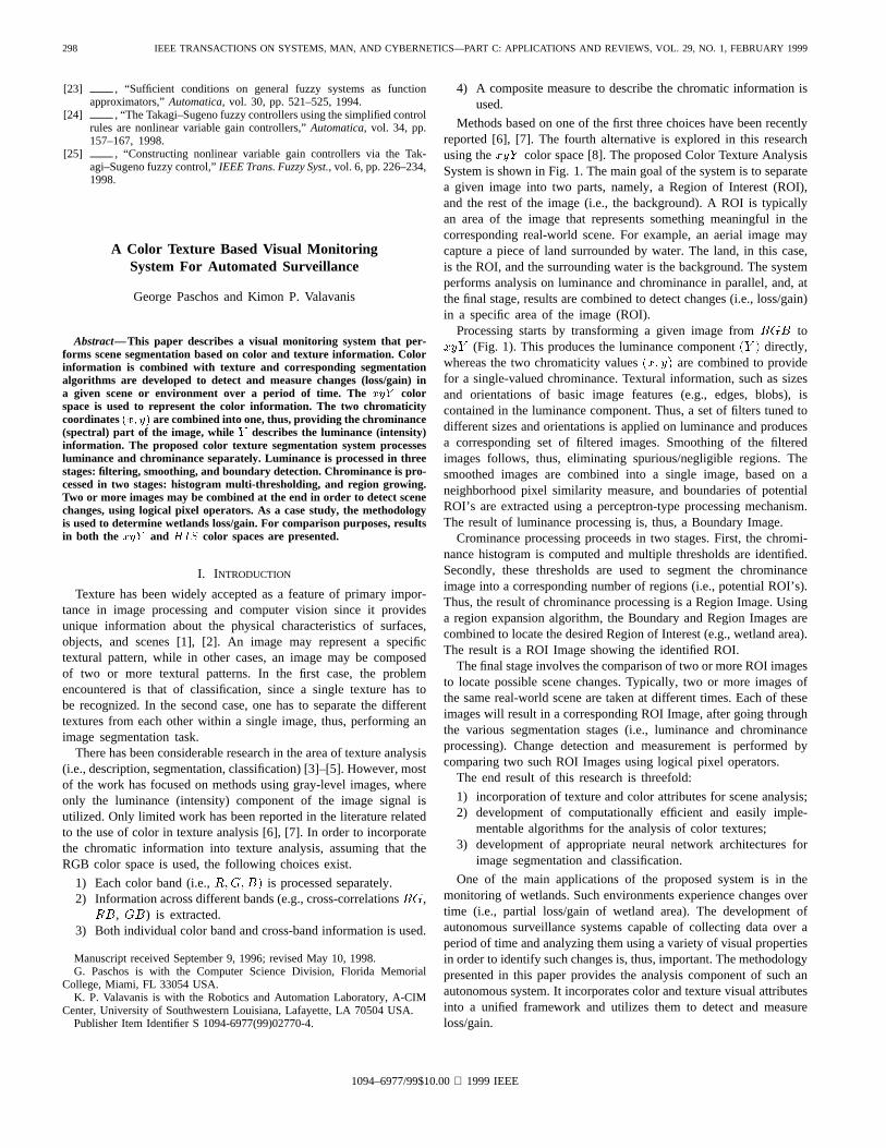
298 IEEE TRANSACTIONS ON SYSTEMS, MAN, AND CYBERNETICS—PART C: APPLICATIONS AND REVIEWS, VOL. 29, NO. 1, FEBRUARY 1999

[23] , “Sufficient conditions on general fuzzy systems as functionapproximators,”Automatica, vol. 30, pp. 521–525, 1994.

[24] , “The Takagi–Sugeno fuzzy controllers using the simplified controlrules are nonlinear variable gain controllers,”Automatica, vol. 34, pp.157–167, 1998.

[25] , “Constructing nonlinear variable gain controllers via the Tak-agi–Sugeno fuzzy control,”IEEE Trans. Fuzzy Syst., vol. 6, pp. 226–234,1998.

A Color Texture Based Visual MonitoringSystem For Automated Surveillance

George Paschos and Kimon P. Valavanis

Abstract—This paper describes a visual monitoring system that per-forms scene segmentation based on color and texture information. Colorinformation is combined with texture and corresponding segmentationalgorithms are developed to detect and measure changes (loss/gain) ina given scene or environment over a period of time. ThexyY colorspace is used to represent the color information. The two chromaticitycoordinates(x; y) are combined into one, thus, providing the chrominance(spectral) part of the image, whileY describes the luminance (intensity)information. The proposed color texture segmentation system processesluminance and chrominance separately. Luminance is processed in threestages: filtering, smoothing, and boundary detection. Chrominance is pro-cessed in two stages: histogram multi-thresholding, and region growing.Two or more images may be combined at the end in order to detect scenechanges, using logical pixel operators. As a case study, the methodologyis used to determine wetlands loss/gain. For comparison purposes, resultsin both the xyY and HIS color spaces are presented.

I. INTRODUCTION

Texture has been widely accepted as a feature of primary impor-tance in image processing and computer vision since it providesunique information about the physical characteristics of surfaces,objects, and scenes [1], [2]. An image may represent a specifictextural pattern, while in other cases, an image may be composedof two or more textural patterns. In the first case, the problemencountered is that of classification, since a single texture has tobe recognized. In the second case, one has to separate the differenttextures from each other within a single image, thus, performing animage segmentation task.

There has been considerable research in the area of texture analysis(i.e., description, segmentation, classification) [3]–[5]. However, mostof the work has focused on methods using gray-level images, whereonly the luminance (intensity) component of the image signal isutilized. Only limited work has been reported in the literature relatedto the use of color in texture analysis [6], [7]. In order to incorporatethe chromatic information into texture analysis, assuming that theRGB color space is used, the following choices exist.

1) Each color band (i.e.,R;G;B) is processed separately.2) Information across different bands (e.g., cross-correlationsRG,

RB, GB) is extracted.3) Both individual color band and cross-band information is used.

Manuscript received September 9, 1996; revised May 10, 1998.G. Paschos is with the Computer Science Division, Florida Memorial

College, Miami, FL 33054 USA.K. P. Valavanis is with the Robotics and Automation Laboratory, A-CIM

Center, University of Southwestern Louisiana, Lafayette, LA 70504 USA.Publisher Item Identifier S 1094-6977(99)02770-4.

4) A composite measure to describe the chromatic information isused.

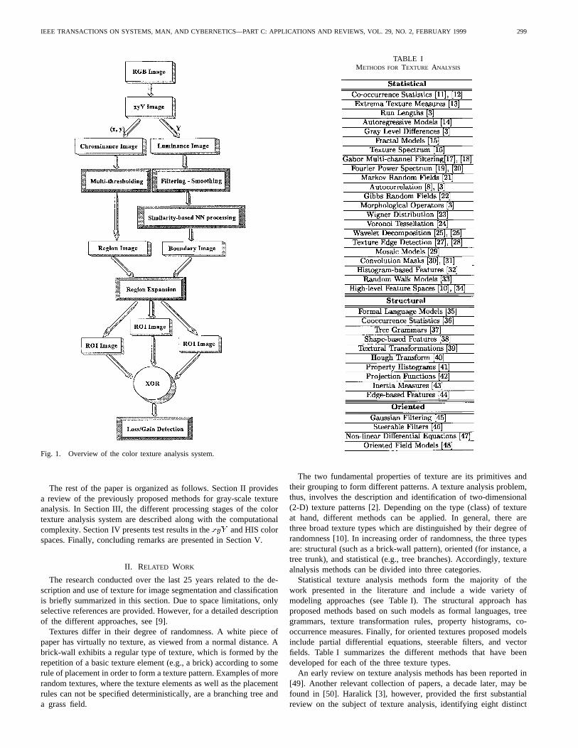
Methods based on one of the first three choices have been recentlyreported [6], [7]. The fourth alternative is explored in this researchusing thexyY color space [8]. The proposed Color Texture AnalysisSystem is shown in Fig. 1. The main goal of the system is to separatea given image into two parts, namely, a Region of Interest (ROI),and the rest of the image (i.e., the background). A ROI is typicallyan area of the image that represents something meaningful in thecorresponding real-world scene. For example, an aerial image maycapture a piece of land surrounded by water. The land, in this case,is the ROI, and the surrounding water is the background. The systemperforms analysis on luminance and chrominance in parallel, and, atthe final stage, results are combined to detect changes (i.e., loss/gain)in a specific area of the image (ROI).

Processing starts by transforming a given image fromRGB toxyY (Fig. 1). This produces the luminance component(Y ) directly,whereas the two chromaticity values(x; y) are combined to providefor a single-valued chrominance. Textural information, such as sizesand orientations of basic image features (e.g., edges, blobs), iscontained in the luminance component. Thus, a set of filters tuned todifferent sizes and orientations is applied on luminance and producesa corresponding set of filtered images. Smoothing of the filteredimages follows, thus, eliminating spurious/negligible regions. Thesmoothed images are combined into a single image, based on aneighborhood pixel similarity measure, and boundaries of potentialROI’s are extracted using a perceptron-type processing mechanism.The result of luminance processing is, thus, a Boundary Image.

Crominance processing proceeds in two stages. First, the chromi-nance histogram is computed and multiple thresholds are identified.Secondly, these thresholds are used to segment the chrominanceimage into a corresponding number of regions (i.e., potential ROI’s).Thus, the result of chrominance processing is a Region Image. Usinga region expansion algorithm, the Boundary and Region Images arecombined to locate the desired Region of Interest (e.g., wetland area).The result is a ROI Image showing the identified ROI.

The final stage involves the comparison of two or more ROI imagesto locate possible scene changes. Typically, two or more images ofthe same real-world scene are taken at different times. Each of theseimages will result in a corresponding ROI Image, after going throughthe various segmentation stages (i.e., luminance and chrominanceprocessing). Change detection and measurement is performed bycomparing two such ROI Images using logical pixel operators.

The end result of this research is threefold:

1) incorporation of texture and color attributes for scene analysis;2) development of computationally efficient and easily imple-

mentable algorithms for the analysis of color textures;3) development of appropriate neural network architectures for

image segmentation and classification.

One of the main applications of the proposed system is in themonitoring of wetlands. Such environments experience changes overtime (i.e., partial loss/gain of wetland area). The development ofautonomous surveillance systems capable of collecting data over aperiod of time and analyzing them using a variety of visual propertiesin order to identify such changes is, thus, important. The methodologypresented in this paper provides the analysis component of such anautonomous system. It incorporates color and texture visual attributesinto a unified framework and utilizes them to detect and measureloss/gain.

1094–6977/99$10.00 1999 IEEE

IEEE TRANSACTIONS ON SYSTEMS, MAN, AND CYBERNETICS—PART C: APPLICATIONS AND REVIEWS, VOL. 29, NO. 2, FEBRUARY 1999 299

Fig. 1. Overview of the color texture analysis system.

The rest of the paper is organized as follows. Section II providesa review of the previously proposed methods for gray-scale textureanalysis. In Section III, the different processing stages of the colortexture analysis system are described along with the computationalcomplexity. Section IV presents test results in thexyY and HIS colorspaces. Finally, concluding remarks are presented in Section V.

II. RELATED WORK

The research conducted over the last 25 years related to the de-scription and use of texture for image segmentation and classificationis briefly summarized in this section. Due to space limitations, onlyselective references are provided. However, for a detailed descriptionof the different approaches, see [9].

Textures differ in their degree of randomness. A white piece ofpaper has virtually no texture, as viewed from a normal distance. Abrick-wall exhibits a regular type of texture, which is formed by therepetition of a basic texture element (e.g., a brick) according to somerule of placement in order to form a texture pattern. Examples of morerandom textures, where the texture elements as well as the placementrules can not be specified deterministically, are a branching tree anda grass field.

TABLE IMETHODS FOR TEXTURE ANALYSIS

The two fundamental properties of texture are its primitives andtheir grouping to form different patterns. A texture analysis problem,thus, involves the description and identification of two-dimensional(2-D) texture patterns [2]. Depending on the type (class) of textureat hand, different methods can be applied. In general, there arethree broad texture types which are distinguished by their degree ofrandomness [10]. In increasing order of randomness, the three typesare: structural (such as a brick-wall pattern), oriented (for instance, atree trunk), and statistical (e.g., tree branches). Accordingly, texturealnalysis methods can be divided into three categories.

Statistical texture analysis methods form the majority of thework presented in the literature and include a wide variety ofmodeling approaches (see Table I). The structural approach hasproposed methods based on such models as formal languages, treegrammars, texture transformation rules, property histograms, co-occurrence measures. Finally, for oriented textures proposed modelsinclude partial differential equations, steerable filters, and vectorfields. Table I summarizes the different methods that have beendeveloped for each of the three texture types.

An early review on texture analysis methods has been reported in[49]. Another relevant collection of papers, a decade later, may befound in [50]. Haralick [3], however, provided the first substantialreview on the subject of texture analysis, identifying eight distinct


statistical and structural methods, used before 1979. Van Gooletal. [4] included some additional methods in their survey of 1983.A more recent review was presented by Reedet al. [5]. Additionalrecent methods may be found in [9].

A particular limitation of the above methods is that they havebeen applied to gray-scale images, thus utilizing only the luminancecomponent of an image. In color vision, the chrominance componentis also of great importance. Chrominance provides additional infor-mation about the viewed scene and, as will be shown in this paper,allows for more effective methods in image segmentation.

In the field of colorimetry, there exist several color systems(spaces) used for the description of color attributes. TheRGB

color space, known for its additive mixture properties that makerepresentation of colors easy, is the most popular. However, dueto practical intrinsic limitations, it is rarely used for color imageprocessing. The main limitation is that theRGB specification ishuman oriented chromatics rather than machine oriented chromatics.Other color spaces adopted by color science include thexyY space,HIS, CIEL�a�b�, CIEL�u�v�, etc. [51]. The NTSC TV System(Y IQ space), for instance, is a typical example of a system derivedfor electronic image transmission and it has been proven to providea better color representation than theRGB space.

Only limited work has been reported in the literature related to theuse of color in texture analysis [6], [7]. All of the approaches haveutilized theRGB color space in order to represent color imagesand perform analysis of the three color channels, namely,R, G, B,separately and in cross-correlation pairs (i.e.,RG, RB, GB). Theprocessing of these six separate information sources imposes severeconstraints on the image processing system in terms of computationalload. A color space that facilitates the use of fewer informationchannels in the processing of color texture images and makesthe separation of luminance and chrominance information easier isdesirable. Utilization of thexyY space, involving the processingof the two channels (i.e., luminance and chrominance) as well astheir interaction, allows for significantly reduced computational costcompared to an approach using theRGB space, as shown in thefollowing sections.

III. COLOR TEXTURE SEGMENTATION

The goal of the proposed system is to separate (segment) a givenimage into two parts, namely, a Region of Interest (ROI), and therest of the image which is regarded as the background. A ROI istypically an area of the image that represents something meaningfulin the corresponding real-world scene. For example, an aerial imagemay capture a piece of land surrounded by water. The land, in thiscase, is the ROI and the surrounding water is the background.

There are two main approaches one can follow in extracting animage region: 1) identify the set of pixels forming the region’s bound-ary (boundary extraction), or 2) identify the set of pixels covering theregion interior (region extraction). The proposed segmentation system(Fig. 1) combines the two approaches in order to compensate forinaccuracies that may result from either approach alone. Specifically,boundary extraction is performed on luminance, while region extrac-tion is performed on chrominance. The region interior extracted fromchrominance is expanded (region expansion) using a pixel similaritycriterion, so that the largest possible image area within the previouslyidentified boundary is covered. This expanded region constitutes aROI that has been completely identified. A ROI image is a black-and-white image where the identified ROI is shown as black, whilethe rest of the image is shown as white (background). Given a setof images taken from a scene at different times, a coresponding setof ROI images is produced by the segmentation system. At the finalstage in the proposed system, the ROI images are combined through

logical pixel operators to reveal possible changes (growth/shrinkage)of the specific region.

Before the different processing stages are described in furtherdetail, the definition of the two image information channels, i.e.,luminance and chrominance, is presented in the following section.

A. Luminance and Chrominance Separation

The proposed system is based on two sources of information,namely, luminance, and chrominance in thexyY color space. Lumi-nance is given byY while chrominance is obtained from thex andychromaticity coordinates through the quantization technique describedbelow. The original images are inRGB and are transformed to theXY Z color space using the following equations [51]:

X = 0:607 �R+ 0:174 �G+ 0:200 �B (1)

Y =0:299 �R+ 0:587 �G+ 0:114 �B (2)

Z =0:066 �G+ 1:111 �B (3)

where the equation forY provides the desired luminance component.The (x; y) chromaticity values are derived from theXY Z color

space ([51]) as follows:

x =X

X + Y + Z(4)

y =Y

X + Y + Z: (5)

The range of values ofx andy is seen to be [0.0, 1.0] indicatingthat the corresponding 2-Dxy space is bounded. If it were alsodiscrete, we could define a one-to-one mapping from a 2-D to a one-dimensional (1-D) space. To provide that property, one may dividethe [0.0, 1.0] interval into a number(k) of equal-length subintervals.Thus, each of thex and y coordinates may take one ofk-discretepossible values, which means that a pair of values may be viewed asa two-digit number in a base-k system. This number can be convertedinto a unique decimal integer, providing the desired 1-D quantity.

Example: If k = 5; i.e., the unit interval is divided into five subin-tervals, the following is the mapping for each of the chromaticitiesindividually:

x; y 2 [0:0; 0:2) 7! h0i

x; y 2 [0:2; 0:4) 7! h1i

x; y 2 [0:4; 0:6) 7! h2i

x; y 2 [0:6; 0:8) 7! h3i

x; y 2 [0:8; 1:0] 7! h4i: (6)

The numbers in the angle brackets are the values to which chro-maticities in the corresponding intervals are mapped. For instance,if x = 0:36, the new value forx, using the above mapping, is 1.Subsequently, a pair of values, is viewed as the numberxy in base-5. For example, ifx = 0:36 andy = 0:78, the corresponding base-5number is 13. This number is mapped to its decimal equivalent usingthe following formula:

cv = y + k � x (7)

wherek is the chosen number of intervals (e.g., 5 in this example),and cv is the desired chrominance value for the particular(x; y)chromaticity pair.

B. Luminance Processing

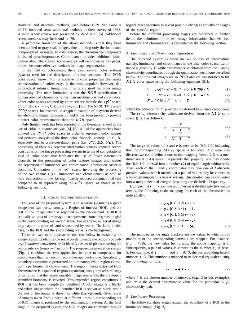
The following three stages extract the boundary of a ROI in theluminance image (Fig. 2).


Fig. 2. Luminance processing component of the color texture analysis sys-tem (see Fig. 1).

1) Filtering: A set of Gabor filters, which are capable of detectingbasic image features (e.g., edges, blobs) at different scales andorientations, is applied on luminance to produce a correspondingnumber of filtered images. The Gabor filters are gaussian-modulatedsinusoidals, defined as follows [18]:

g(m;n) = e�(m +n =2� )

e�2j��(m cos �+n sin �) (8)

where m;n are the pixel coordinates,�2 is the variance of theGaussian function, and� and� represent the filter tuning parameters,namely, orientation and spatial frequency of the complex exponential,respectively.

The real part of the complex exponential is used in this method,thus, reducing the computational cost while not affecting its detectioncapabilities, and is defined as follows:

g(m;n) = e�(m +n =2� ) cos(2��(m cos � + n sin �)): (9)

Based on experimental evaluation, two orientations (0� and 90�) andtwo frequencies (0.25 and 0.50) have been selected, as they provideadequate detection capabilities for images in the particular applicationdomain (i.e., wetland scenes) while keeping the computational costlow. Four filters are, thus, created and applied to the luminanceimage. However, if different applications are sought, additionalfrequencies/orientations may be used. Since each of the differentfilter orientations and frequencies allows for the detection of imagefeatures of specific directionality and size, one may use more thanthose suggested here to capture finer/coarser details in a given image.Thus, a trade-off exists between the imposed computational load, i.e.,the number of orientations and frequencies that are to be processed,and the degree of image detail deemed adequate in a particularapplication. As a result of the application of these four filters (i.e.,two spatial frequencies, and two orientations) to the luminance image,four corresponding filtered images are produced.

2) Smoothing: Iterative smoothing using a3�3 window is appliedto each of the four filtered images produced by filtering at stage 1, sothat spurious (random) image variations are removed and the majorregions in the image become more prominent. Based on experimentalobservations, three iterations are usually sufficient.

3) Boundary Detection:A single-level neural network (one-layerperceptron) is subsequently employed, that combines the smoothedfilter outputs to produce a single boundary image. The neural netarchitecture includes one node per pixel and eight inputs per node.

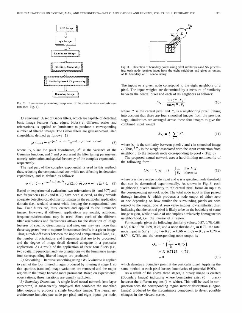
Fig. 3. Detection of boundary points using pixel similarities and NN process-ing: each node receives input from the eight neighbors and gives an outputof 0: boundary or 1: nonboundary.

The inputs to a given node correspond to the eight neighbors of apixel. The input weights are determined by a measure of similaritybetween the central pixel and each of its neighbors as follows:

Sij =min(Pi; Pj)

max(Pi; Pj(10)

wherePi is the central pixel andPj is a neighboring pixel. Takinginto account that there are four smoothed images from the previousstage, similarities are averaged across these four images to give thecombined input weight

Wij =14

4

k=1

Skij (11)

whereSkij is the similarity between pixelsi andj in smoothed imagek: Thus,Wij is the weight associated with the input connection fromneighborj to the network node corresponding to pixeli (Fig. 3).

The proposed neural network uses a hard-limiting nonlinearity ofthe following form:

ON = K(�� ) =1; if � � �

0; otherwise(12)

where� is the average node input and� is a specified node thresholdthat can be determined experimentally. As shown in Fig. 3, eachneighboring pixel’s similarity to the central pixel forms an input tothe corresponding network node. The total node input is then passedthrough functionK which produces a node output of either zeroor one depending on how similar the surrounding pixels are withrespect to the central one. A zero value implies low similarity, thus,indicating that the central pixel is likely to be on the boundary of someimage region, while a value of one implies a relatively homogeneousneighborhood, i.e., the interior of a region.

For example, given the following similarity values, 0.57, 0.75, 0.66,0.55, 0.82, 0.70, 0.89, 0.76, and a node threshold� = 0:75; the totalnode input is 5.7(= 0:57 + 0:75 + 0:66 + 0:55 + 0:82 + 0:70 +0:89 + 0:76), and the corresponding node output is:

ON =K5:7

8� 0:75

=K(0:7125� 0:75)

=0 (13)

which denotes a boundary point at the particular pixel. Applying thesame method at each pixel locates boundaries of potential ROI’s.

As a result of the above three stages, a binary image is created(Boundary Image) indicating where boundaries exist (0= black)between the different regions (1= white). This will be used in con-junction with the corresponding region interior description (RegionImage) produced by the chrominance component to detect possiblechanges in the viewed scene.


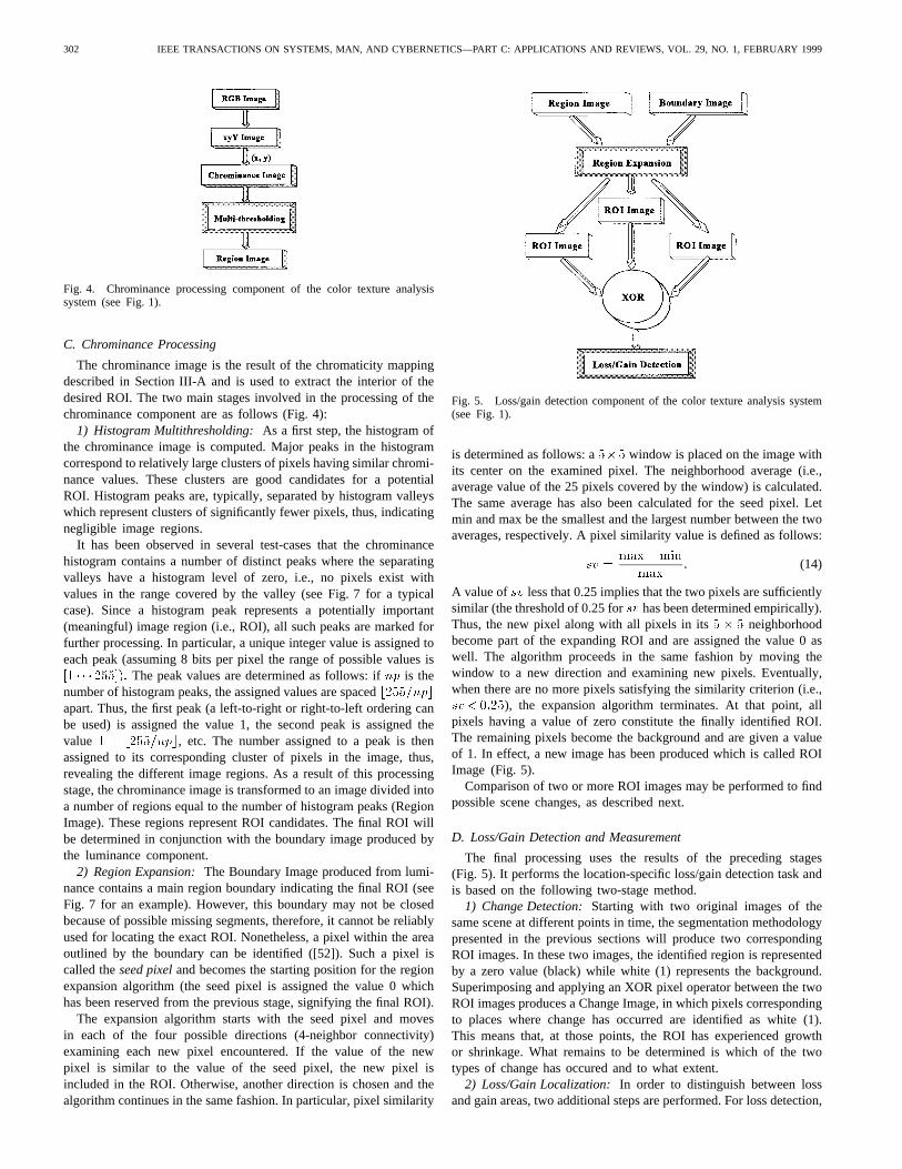
Fig. 4. Chrominance processing component of the color texture analysissystem (see Fig. 1).

C. Chrominance Processing

The chrominance image is the result of the chromaticity mappingdescribed in Section III-A and is used to extract the interior of thedesired ROI. The two main stages involved in the processing of thechrominance component are as follows (Fig. 4):

1) Histogram Multithresholding:As a first step, the histogram ofthe chrominance image is computed. Major peaks in the histogramcorrespond to relatively large clusters of pixels having similar chromi-nance values. These clusters are good candidates for a potentialROI. Histogram peaks are, typically, separated by histogram valleyswhich represent clusters of significantly fewer pixels, thus, indicatingnegligible image regions.

It has been observed in several test-cases that the chrominancehistogram contains a number of distinct peaks where the separatingvalleys have a histogram level of zero, i.e., no pixels exist withvalues in the range covered by the valley (see Fig. 7 for a typicalcase). Since a histogram peak represents a potentially important(meaningful) image region (i.e., ROI), all such peaks are marked forfurther processing. In particular, a unique integer value is assigned toeach peak (assuming 8 bits per pixel the range of possible values is[1 � � � 255]): The peak values are determined as follows: ifnp is thenumber of histogram peaks, the assigned values are spacedb255=npc

apart. Thus, the first peak (a left-to-right or right-to-left ordering canbe used) is assigned the value 1, the second peak is assigned thevalue 1 + b255=npc, etc. The number assigned to a peak is thenassigned to its corresponding cluster of pixels in the image, thus,revealing the different image regions. As a result of this processingstage, the chrominance image is transformed to an image divided intoa number of regions equal to the number of histogram peaks (RegionImage). These regions represent ROI candidates. The final ROI willbe determined in conjunction with the boundary image produced bythe luminance component.

2) Region Expansion:The Boundary Image produced from lumi-nance contains a main region boundary indicating the final ROI (seeFig. 7 for an example). However, this boundary may not be closedbecause of possible missing segments, therefore, it cannot be reliablyused for locating the exact ROI. Nonetheless, a pixel within the areaoutlined by the boundary can be identified ([52]). Such a pixel iscalled theseed pixeland becomes the starting position for the regionexpansion algorithm (the seed pixel is assigned the value 0 whichhas been reserved from the previous stage, signifying the final ROI).

The expansion algorithm starts with the seed pixel and movesin each of the four possible directions (4-neighbor connectivity)examining each new pixel encountered. If the value of the newpixel is similar to the value of the seed pixel, the new pixel isincluded in the ROI. Otherwise, another direction is chosen and thealgorithm continues in the same fashion. In particular, pixel similarity

Fig. 5. Loss/gain detection component of the color texture analysis system(see Fig. 1).

is determined as follows: a5�5 window is placed on the image withits center on the examined pixel. The neighborhood average (i.e.,average value of the 25 pixels covered by the window) is calculated.The same average has also been calculated for the seed pixel. Letmin and max be the smallest and the largest number between the twoaverages, respectively. A pixel similarity value is defined as follows:

sv =max�min

max: (14)

A value ofsv less that 0.25 implies that the two pixels are sufficientlysimilar (the threshold of 0.25 forsv has been determined empirically).Thus, the new pixel along with all pixels in its5� 5 neighborhoodbecome part of the expanding ROI and are assigned the value 0 aswell. The algorithm proceeds in the same fashion by moving thewindow to a new direction and examining new pixels. Eventually,when there are no more pixels satisfying the similarity criterion (i.e.,sv < 0:25), the expansion algorithm terminates. At that point, allpixels having a value of zero constitute the finally identified ROI.The remaining pixels become the background and are given a valueof 1. In effect, a new image has been produced which is called ROIImage (Fig. 5).

Comparison of two or more ROI images may be performed to findpossible scene changes, as described next.

D. Loss/Gain Detection and Measurement

The final processing uses the results of the preceding stages(Fig. 5). It performs the location-specific loss/gain detection task andis based on the following two-stage method.

1) Change Detection:Starting with two original images of thesame scene at different points in time, the segmentation methodologypresented in the previous sections will produce two correspondingROI images. In these two images, the identified region is representedby a zero value (black) while white (1) represents the background.Superimposing and applying an XOR pixel operator between the twoROI images produces a Change Image, in which pixels correspondingto places where change has occurred are identified as white (1).This means that, at those points, the ROI has experienced growthor shrinkage. What remains to be determined is which of the twotypes of change has occured and to what extent.

2) Loss/Gain Localization:In order to distinguish between lossand gain areas, two additional steps are performed. For loss detection,


an AND pixel operator is applied between the first of the two ROIimages (i.e., the one corresponding to an original image taken at anearlier time), and the Change Image produced at the previous stage. Ifany change over part of the identified ROI (first image) is detected, itis of type loss. On the other hand, applying an AND operator betweenthe second image (i.e., corresponding to a later time) and the ChangeImage reveals the areas where gain has occurred.

Since change is designated by the value of 1 while the rest ofthe image has been assigned the value of 0, it is a straightforwardtask to count the number of pixels representing change and find thepercentage of loss/gain relative to the first of the two images.

E. Implementation in the HIS Color Space

For comparison purposes, the segmentation system described abovehas been also implemented in theHIS color space whose threeprimaries, Hue(H), Intensity (I), Saturation(S), provide a morehuman-oriented system for color description.

In order to have a two-channel vision system in theHIS space,HandI will be utilized only. Different definitions forHIS have beenproposed (see [52], [2]). In [53], the following definition is used forhue (based on theRGB space):

H = arctan( (3)(G�B)=(2 �R�G�B)): (15)

The apparent singularity occurs whenR = G = B in which caseboth the numerator and the denominator of the fraction are zero andthe function becomes undefined. The implementation used in thissection follows that of [53] but with a minor modification, in orderto avoid the singularity

I =R+G+B

3(16)

H = arctan(p3(G� 2 �B)=(2 �R�G�B)): (17)

Only whenR = G = B = 0; will there be a singularity point.In such a case, the value assigned toH is zero which, naturally,signifies black.

In order to quantizeH (i.e., in [0..255]) so that its values can beassigned as pixel values (8 bits per pixel), and given that the rangeof arctan values is[0 � � ��]; the following equations are used:

H1 =180 �H + 180 (18)

H2 =H1

1:406: (19)

First, the transformation to [0� � � �360�] (i.e., radians to degrees)is performed (18), followed by the mapping of [0� � �360�] to [0��255] (19). In effect,H2 is utilized as an equivalent to the combinedxy chromaticity measure introduced in thexyY space (7), whileIrepresents luminance.

F. Computational Complexity

In this section, the computational complexity is derived for eachof the individual processing modules that comprise the segmentationsystem and the combined complexity for the execution of the entiresegmentation task is determined. The computational complexity isdefined in terms of the number of pixels visited, i.e., the number oftimes the value of a pixel needs to be accessed/used in an operation,such as comparisons and multiplications/divisions. In what follows,anN �N square image is assumed as input to the system.

The filtering part requires the application of four filters on a givenimage. Each individual filter accesses every pixel and performs aneighborhood-type summation over a windoww where each pixel inthe neighborhood is multiplied by the corresponding filter weight (9)and the total sum becomes the new value of the central pixel. Since

the window is typically of odd size (so that a central pixel exists),there is a strip of pixels(w � 1)=2-wide on each side of the imagethat cannot become centers of a window (that is, a window cannotbe placed at those positions without falling outside the image area).Therefore, the image area that is actually processed is(N �w+1)2

pixels. At each pixel, neighborhood processing needsw2 operations.Filtering as whole (i.e., four filters) requires the following numberof operations:

T1 = 4 � (N � w + 1)2 �w2: (20)

Smoothing follows filtering and, in a similar way, it processes eachof the four filter images with a window-type operation (assuming awindow of the same size) and, thus, performs the same number ofoperations:

T2 = 4 � (N � w + 1)2 �w2: (21)

In order to calculate the pixel similarities (10), two operationsare performed, namely, a comparison between the two pixels to findthe minimum and maximum values, and a division. However, sincecomplexity is measured at the pixel level, that is, what counts isthe number of pixels visited and not how many and of what typeoperations are applied at each pixel, each similarity calculation countsas one operation. Consequently, since this is done for each of theneighborhood pixels except for the central one, and, also, over thefour smoothed images, the resulting number of operations is:

T3 = 4 � (N � w + 1)2 � (w2 � 1): (22)

As a side note,T3 can be reduced if one notices that similaritiesbetween any two pixels are calculated twice as the window movesfrom one pixel to another. A more efficient algorithm can be devisedthat keeps track of the pixels that have already been visited by themoving window and, thus, avoid recalculating the correspondingsimilarities. Although the current implementation does not includethat, it is easy to make the modification.

For the boundary detection, the single similarity image is pro-cessed with a similar window operation and based on the precedingdiscussion, the number of operations for the entire image is

T4 = 4 � (N � w + 1)2 �w2: (23)

Combining the last four equations, the total cost for luminanceprocessing is

TL = (N � w + 1)2 � (10 �w2 � 1): (24)

The processing of chrominance involves the computation of thechrominance histogram, thresholding, ROI extraction, and applicationof the XOR operator for change localization. Each of these steps visitsevery pixel except for the ROI extraction stage which visits as manypixels as there are in the ROI. Since this is a variable quantity anddepends on the particular image at hand, it is assumed that a portion�of the entire image is visited. As a result, the combined chrominanceprocessing system performs the following number of pixel operations

TC = (3 + �) �N2: (25)

The following, then, holds for the combined processing cost.Result: The segmentation system has a complexity ofO(b �N);

where b = 10 � w2 + 2 � �:Based on the above analysis, the following can be proven.


(a) (b)

(c)

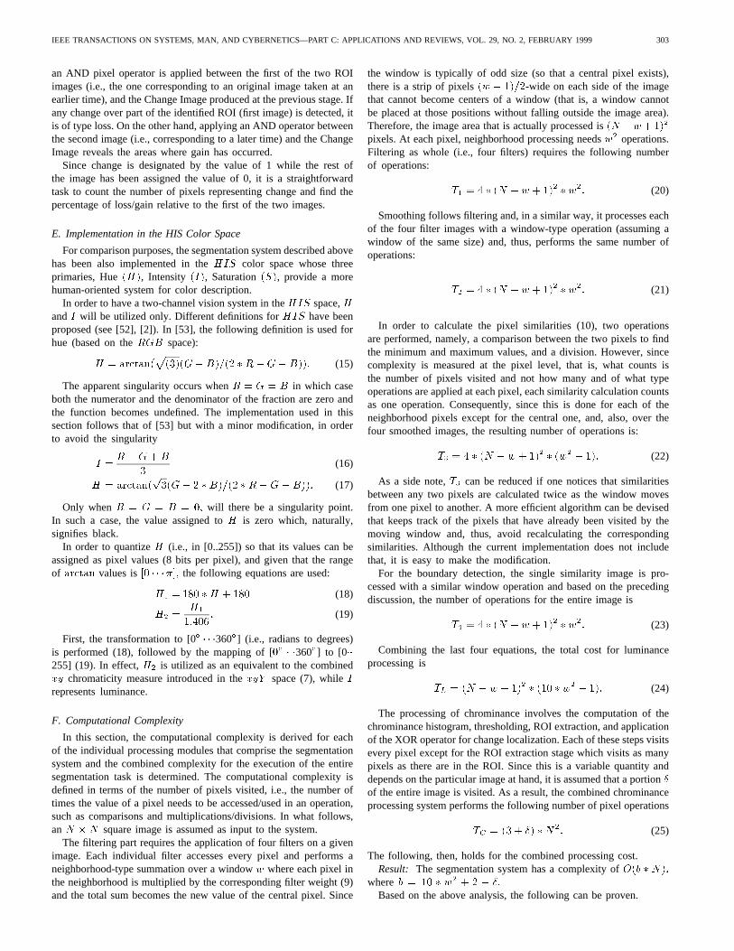
Fig. 6. (a), (b) The original wetland images. (c) Loss/gain detection between the first and the second wetland images(xyY space), where the top two arethe segmentation results (i.e., the two ROI Images), and at the bottom is the Change Image (loss in black, and gain in medium gray—light gray is the restof the image, i.e., the background). (Color versions of this figure can be obtained by contacting G. Paschos).

Lemma: The proposed two-channelxyY -based segmentation sys-tem requires less number of pixel operations than an equivalentthree-channelRGB-based scheme.

Proof: It is assumed that one of the three color primaries (forinstanceB) is used for the luminance processing part while theother two (i.e.,R;G) are processed using the chrominance algorithms(if only one of them is used in chrominance processing, significantinformation may be lost). The cost, then, for this system is:

TRGB = 2 � TC + TL (26)

whereas the total cost for the proposed system, including the trans-formations (Ttr) from RGB to XY Z to xyY along with thechromaticity mapping, is:

TxyY = Ttr + TC + TL (27)

Since each of the three transformations costs has a cost ofN2

pixel operations, the cost difference between the two systems is:

�T =TRGB + TxyY

=TC + Ttr

=(3 + �) �N2� 3 �N2

= � �N2 (28)

Typically, the ROI may occupy 30–50% of the image area. Forinstance, if the specific ROI covers 35% of a64 � 64 image, then� = 0:35 ) �T = 0:35 � 642 = 1433:6 which means thatthere is a processing gain of 1433.6 pixel operations (35%). Thus,the absolute advantage of the proposed system (number of pixeloperations) depends on the size of the processed image and the size ofthe ROI, while the relative advantage (percent of ROI area) dependson the ROI at hand.


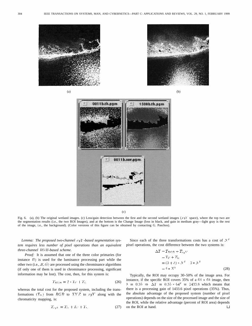
Fig. 7. Segmentation results from the first wetland image inxyY:Top-to-bottom: four filtered images (row 1), four smoothed images (row 2),Region Image-Boundary Image-ROI Image (row 3, left-to-right), chrominancehistogram (bottom).

In the HIS space, the same algorithms have been used. Theonly modification, as shown in the results, is the use of histogramequalization as a preprocessing step in order to obtain a more balancedhue image, in terms of pixel value distribution. Thus, the samecomplexity results hold, as in thexyY space.

IV. RESULTS

Several aerial images of wetland scenes have been used for testingthe proposed system. Two such images are shown in Fig. 6(a) and(b). The segmentation system (Section III-A-C) has been applied toeach of these images and the results obtained are shown in Figs. 7and 8 for thexyY color space, and Figs. 9 and 10 for theHIS space.

Let’s consider the segmentation results for the first image[Fig. 6(a)] as shown in Fig. 7. The results after Gabor filtering(Section III-B, stage 1) are shown as the top four images. Thesefiltered images are slightly different among each other in terms ofthe image areas they have emphasized, due to the different scales andorientations of the Gabor filters used. For instance, a small fragmentof the wetland area may have been missed by one filter but detectedby another and vice versa. As a whole, the wetland area has beenadequately exposed with respect to the surrounding water area. Abright spot, due to reflection from an artificial light source, has alsobeen detected and forms a potential second major region (i.e., ROI).However, this second region will be eliminated in the subsequentstages both because of its incoherence (i.e., many nonbright pixels,belonging to the water area, within this pixel cluster), and due tosuccessful selection of neural-net cutoff thresholds (12).

The second quadruple of images in Fig. 7 (second row) shows theresults of smoothing (Section III-B, stage 2). The two main regions

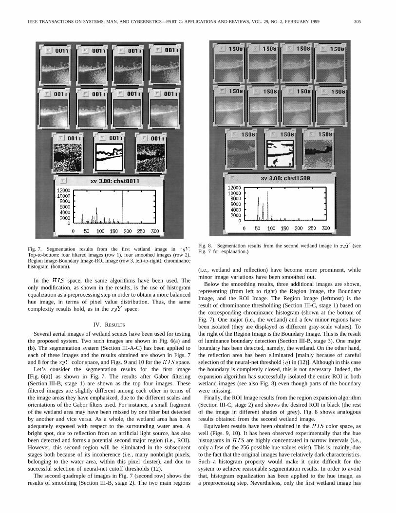
Fig. 8. Segmentation results from the second wetland image inxyY (seeFig. 7 for explanation.)

(i.e., wetland and reflection) have become more prominent, whileminor image variations have been smoothed out.

Below the smoothing results, three additional images are shown,representing (from left to right) the Region Image, the BoundaryImage, and the ROI Image. The Region Image (leftmost) is theresult of chrominance thresholding (Section III-C, stage 1) based onthe corresponding chrominance histogram (shown at the bottom ofFig. 7). One major (i.e., the wetland) and a few minor regions havebeen isolated (they are displayed as different gray-scale values). Tothe right of the Region Image is the Boundary Image. This is the resultof luminance boundary detection (Section III-B, stage 3). One majorboundary has been detected, namely, the wetland. On the other hand,the reflection area has been eliminated [mainly because of carefulselection of the neural-net threshold(�) in (12)]. Although in this casethe boundary is completely closed, this is not necessary. Indeed, theexpansion algorithm has successfully isolated the entire ROI in bothwetland images (see also Fig. 8) even though parts of the boundarywere missing.

Finally, the ROI Image results from the region expansion algorithm(Section III-C, stage 2) and shows the desired ROI in black (the restof the image in different shades of grey). Fig. 8 shows analogousresults obtained from the second wetland image.

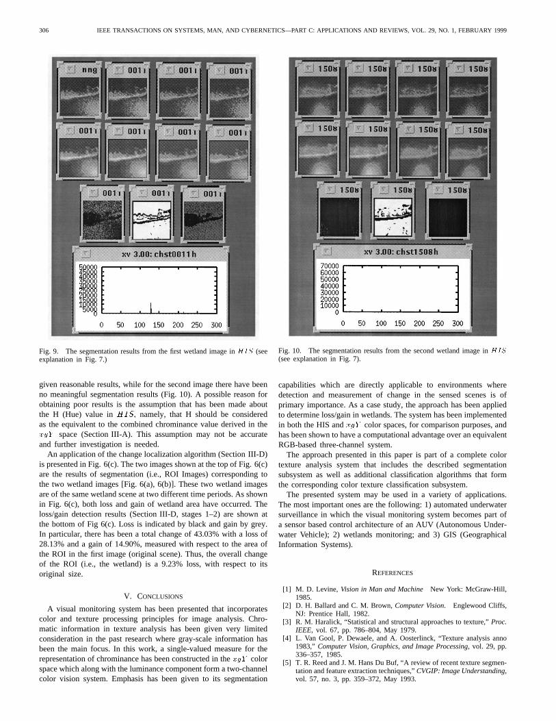
Equivalent results have been obtained in theHIS color space, aswell (Figs. 9, 10). It has been observed experimentally that the huehistograms inHIS are highly concentrated in narrow intervals (i.e.,only a few of the 256 possible hue values exist). This is, mainly, dueto the fact that the original images have relatively dark characteristics.Such a histogram property would make it quite difficult for thesystem to achieve reasonable segmentation results. In order to avoidthat, histogram equalization has been applied to the hue image, asa preprocessing step. Nevertheless, only the first wetland image has


Fig. 9. The segmentation results from the first wetland image inHIS (seeexplanation in Fig. 7.)

given reasonable results, while for the second image there have beenno meaningful segmentation results (Fig. 10). A possible reason forobtaining poor results is the assumption that has been made aboutthe H (Hue) value inHIS; namely, that H should be consideredas the equivalent to the combined chrominance value derived in thexyY space (Section III-A). This assumption may not be accurateand further investigation is needed.

An application of the change localization algorithm (Section III-D)is presented in Fig. 6(c). The two images shown at the top of Fig. 6(c)are the results of segmentation (i.e., ROI Images) corresponding tothe two wetland images [Fig. 6(a), 6(b)]. These two wetland imagesare of the same wetland scene at two different time periods. As shownin Fig. 6(c), both loss and gain of wetland area have occurred. Theloss/gain detection results (Section III-D, stages 1–2) are shown atthe bottom of Fig 6(c). Loss is indicated by black and gain by grey.In particular, there has been a total change of 43.03% with a loss of28.13% and a gain of 14.90%, measured with respect to the area ofthe ROI in the first image (original scene). Thus, the overall changeof the ROI (i.e., the wetland) is a 9.23% loss, with respect to itsoriginal size.

V. CONCLUSIONS

A visual monitoring system has been presented that incorporatescolor and texture processing principles for image analysis. Chro-matic information in texture analysis has been given very limitedconsideration in the past research where gray-scale information hasbeen the main focus. In this work, a single-valued measure for therepresentation of chrominance has been constructed in thexyY colorspace which along with the luminance component form a two-channelcolor vision system. Emphasis has been given to its segmentation

Fig. 10. The segmentation results from the second wetland image inHIS

(see explanation in Fig. 7).

capabilities which are directly applicable to environments wheredetection and measurement of change in the sensed scenes is ofprimary importance. As a case study, the approach has been appliedto determine loss/gain in wetlands. The system has been implementedin both the HIS andxyY color spaces, for comparison purposes, andhas been shown to have a computational advantage over an equivalentRGB-based three-channel system.

The approach presented in this paper is part of a complete colortexture analysis system that includes the described segmentationsubsystem as well as additional classification algorithms that formthe corresponding color texture classification subsystem.

The presented system may be used in a variety of applications.The most important ones are the following: 1) automated underwatersurveillance in which the visual monitoring system becomes part ofa sensor based control architecture of an AUV (Autonomous Under-water Vehicle); 2) wetlands monitoring; and 3) GIS (GeographicalInformation Systems).

REFERENCES

[1] M. D. Levine, Vision in Man and Machine New York: McGraw-Hill,1985.

[2] D. H. Ballard and C. M. Brown,Computer Vision. Englewood Cliffs,NJ: Prentice Hall, 1982.

[3] R. M. Haralick, “Statistical and structural approaches to texture,”Proc.IEEE, vol. 67, pp. 786–804, May 1979.

[4] L. Van Gool, P. Dewaele, and A. Oosterlinck, “Texture analysis anno1983,” Computer Vision, Graphics, and Image Processing, vol. 29, pp.336–357, 1985.

[5] T. R. Reed and J. M. Hans Du Buf, “A review of recent texture segmen-tation and feature extraction techniques,”CVGIP: Image Understanding,vol. 57, no. 3, pp. 359–372, May 1993.


[6] T. Caelli and D. Reye, “On the classification of image regions by color,texutre and shape,”Pattern Recognit., no. 4, pp. 461–470, 1993.

[7] R. Kondepudy and G. Healy, “Modeling and identifying 3-D colortextures,” inProc. Int. Conf. Computer Vision and Pattern Recognition,1993, pp. 577–582.

[8] G. Paschos and K. P. Valavanis, “Chromatic features for color texturedescription and analysis,” inIEEE Int. Symp. Intelligent Control, Aug.1995, pp. 319–325.

[9] G. Paschos, “Color and texture based image analysis: Segmentationand classification,” Ph.D. dissertation, Center for Advanced ComputerStudies, Univ. Southwestern Louisiana, Lafayette, LA, May 1996.

[10] A. R. Rao and G. L. Lohse, “Identifying high level features of textureperception,”CVGIP: Graph. Models Image Process., vol. 55, no. 3, pp.218–233, May 1993.

[11] S. Houzelle and G. Giraudon, “Model based region segmentation usingcooccurrence matrices,” inProc. Int. Conf. Computer Vision and PatternRecognition, 1992, pp. 626–639.

[12] L. S. Davis, S. A. Johns, and J. K. Aggarwal, “Texture analysisusing generalized co-occurrence matrices,”IEEE Trans. Pattern Anal.Machine Intell., vol. PAMI-1, pp. 251–259, Mar. 1979.

[13] O. R. Mitchell and S. G. Carlton, “Image segmentation using a localextrema texture measure,”Pattern Recognit., vol. 10, 1978, pp. 205–210.

[14] P. D. Souza, “Texture recognition via autoregression,”Pattern Recognit.,vol. 14, no. 6, pp. 471–475, 1982.

[15] A. Pentland, “Fractal-based description of natural scenes,”IEEE Trans.Pattern Anal. Machine Intell., vol. PAMI-6, pp. 661–674, June 1984.

[16] D. C. He and L. Wang, “Texture features based on texture spectrum,”Pattern Recognit., vol. 23, no. 5, pp. 391–399, 1991.

[17] A. C. Bovik, M. Clark, and W. S. Geisler, “Multichannel texture analysisusing localized spatial filters,”IEEE Trans. Pattern Anal. MachineIntell., vol. 12, pp. 55–73, Jan. 1990.

[18] A. K. Jain and F. Farrokhnia, “Unsupervised texture segmentation usinggabor filters,”Pattern Recognit., vol. 23, no. 12, pp. 1167–1186, 1991.

[19] S. T. Tanimoto, “An optimal algorithm for computing fourier texturedescriptors,”IEEE Trans. Comput., vol. C-27, pp. 81–86, Jan. 1977.

[20] R. Bajcsy, “Computer description of textured surfaces,” inProc. Int.Joint Conf. Artificial Intelligence, 1973, pp. 572–579.

[21] G. R. Cross and A. K. Jain, “Markov random field texture models,”IEEETrans. Pattern Anal. Machine Intell., vol. PAMI-5, pp. 25–39, Jan. 1983.

[22] H. Derin and W. S. Cole, “Segmentation of textured images using Gibbsrandom fields,”Comput. Vis., Graph. Image Process., vol. 35, pp. 72–98,1986.

[23] T. R. Reed and H. Wechsler, “Segmentation of textured images sen-tations,” IEEE Trans. Pattern Anal. Machine Intell., vol. 12, pp. 1–12,Jan. 1990.

[24] M. Tuceryan and A. K. Jain, “Texture segmentation using Voronoipolygons,”IEEE Trans. Pattern Anal. Machine Intell., vol. PAMI-1, pp.211–216, Feb. 1990.

[25] T. Chang and C. C. J. Kuo, “Texture analysis and classification with tree-structured wavelet transforms,”IEEE Trans. Image Processing, vol. 2,pp. 429–441, Oct. 1993.

[26] S. G. Mallat, “A theory of multiresolution signal decomposition: Thewavelet representation,”IEEE Trans. Pattern Anal. Machine Intell., vol.11, pp. 674–693, July 1989.

[27] L. S. Davis and A. Mitiche, “Edge detection in textures,” inComput.Graph. Image Processing, vol. 12, pp. 25–39, 1980.

[28] Y. Xiaohan, J. Yla-Jaaski, and Y. Baozong, “A new algorithm for texturesegmentation based on edge detection,”Pattern Recognit., no. 11, pp.1105–1112, 1991.

[29] N. Ahuja and A. Rozenfeld, “Mosaic models for texture,”IEEE Trans.Pattern Anal. Machine Intell., vol. PAMI-3, pp. 1–11, Jan. 1981.

[30] K. K. Benke, D. R. Skinner, and C. J. Woodruff, “Convolution operatorsas a basis for objective correlates of texture perception,”IEEE Trans.Syst., Man, Cybern., vol. 18, pp. 158–163, Jan./Feb. 1988.

[31] J. Y. Hsiao and A. A. Sawchuk, “Unsupervised textured image segmen-tation using feature smoothing and probabilistic relaxation techniques,”Comput. Vis., Graph. Image Process., vol. 48, pp. 1–21, 1989

[32] M. Unser, “Sum and difference histograms for texture classification,”IEEE Trans. Pattern Anal. Machine Intell., vol. PAMI-8, pp. 118–125,Jan. 1986.

[33] H. Wechsler and M. Kidode, “A random walk procedure for texturediscrimination,”IEEE Trans. Pattern Anal. Machine Intell., vol. PAMI-1,pp. 272–280, July 1979.

[34] A. Amadasun and R. King, “Textural features corresponding to texturalproperties,”IEEE Trans. Syst., Man, Cybern., vol. 19, pp. 1264–1273,Sept./Oct. 1989.

[35] L. Carlucci, “A formal system for texture languages,”Pattern Recognit.,vol. 4, pp. 53–72, 1972.

[36] S. W. Zucker and D. Terzopoulos, “Finding structure in co-occurrencematrices for texture analysis,”Comput. Graph. Image Process., vol. 12,pp. 286–308, 1980.

[37] S. Y. Lu and K. S. Fu, “A syntactic approach to texture analysis,”Comput. Graph. Image Process., vol. 7, pp. 303–330, 1978.

[38] J. G. Leu and W. G. Wee, “Detecting the spatial structure of naturaltextures based on shape analysis,”Comput. Vis., Graph. Image Process.,vol. 31, pp. 67–88., 1985.

[39] S. W. Zucker, “Toward a model of texture,”Comput. Graph. ImageProcess., vol. 5, pp. 190–202, 1976.

[40] G. Eichmann and T. Kasparis, “Topologically inariant texture descrip-tors,” Comput. Vis., Graph. Image Process., vol. 41, 1988, pp. 267–281.

[41] S. Tsuji and F. Tomita, “A structural analyzer for a class of textures,”Comput. Graph. Image Process., vol. 2, pp. 216–231, 1973.

[42] H. B. Kim and R. H. Park, “Extracting spatial arrangement of structuraltextures using projection information,”Pattern Recognit., no. 3, pp.237–245, 1992.

[43] R. W. Conners and C. A. Harlow, “Toward a structural textural analyzerbased on statistical methods,”Comput. Graph. Image Process., vol. 12,pp. 224–256, 1980.

[44] T. H. Hong, C. Dyer, and A. Rosenfeld, “Texture primitive extractionusing an edge-based approach,”IEEE Trans. Syst., Man, Cybern., vol.SMC-10, pp. 659–675, Oct. 1980.

[45] A. R. Rao and R. C. Jain, “Computerized flow field analysis: Orientedtexture patterns,”IEEE Trans. Pattern Anal. Machine Intell., vol. 14,pp. 693–709, July 1992.

[46] W. T. Freeman and E. H. Adelson, “The design and use of steerablefilters,” IEEE Trans. Pattern Anal. Machine Intell., vol. 13, pp. 891–906,Sept. 1991.

[47] R. M. Ford and R. N. Strickland, “Nonlinear phase portrait modelsfor oriented textures,” inProc. Int. Conf. Computer Vision and PatternRecognition, 1993, pp. 644–645.

[48] C. F. Shu and R. C. Jain, “Vector field analysis for oriented patterns,”in Proc. Int. Conf. Computer Vision and Pattern Recognition, 1993, pp.673–676.

[49] B. S. Lipkin and A. Rosenfield,Picture Processing and Psychopictorics.New York: Academic, 1970.

[50] A. Rosenfield,Image Modeling. New York: Academic, 1971.[51] G. W. Wyszecki and S. W. Stiles,Color Science: Concepts and Methods,

Quantitative Data and Formulas. New York: Wiley, 1982.[52] W. K. Pratt,Digital Image Processing. New York: Wiley, 1991.[53] F. Perez, “Hue segmentation, VLSI circuits, and the Mantis shrimp,”

Ph.D. dissertation, California Institute of Technology, Pasadena, CA,1995.

A color texture based visual monitoring system for automated surveillance

Documents

Transcript of A color texture based visual monitoring system for automated surveillance