Spatial Statistics ( ) –

Contents lists available at ScienceDirect

Spatial Statistics

journal homepage: www.elsevier.com/locate/spasta

A closer look at the spatial exponentialmatrix specificationErica Rodrigues a,∗, Renato Assunção b, Dipak K. Dey c

a Departamento de Estatística, Universidade Federal de Ouro Preto, Diogo de Vasconcelos, 122, Ouro Preto,Brazilb Departamento de Ciência da Computação, Universidade Federal de Minas Gerais,Avenida Antônio Carlos, 6627, Belo Horizonte, Brazilc 215 Glenbrook Road, University of Connecticut, Storrs, CT 06269-4098, United States

a r t i c l e i n f o

Article history:Received 30 August 2013Accepted 28 November 2013Available online xxxx

Keywords:Exponential matrixSpatial autoregressionCovariance matrixSpatial regression

a b s t r a c t

In this paper we analyze the partial and marginal covariancestructures of the spatial model with the covariance structurebased on a exponential matrix specification. We show that thismodel presents a puzzling behavior formany types of geographicalneighborhood graphs, from the simplest to the most complex. Inparticular, we show that for this model it is usual to have oppositesigns for the marginal and conditional correlations between twoareas. We show these results through experimental examples andanalytical demonstrations.

© 2013 Elsevier B.V. All rights reserved.

1. Introduction

Suppose we have a region R partitioned into n disjoint areas A1, A2, . . . , An such that ∪ni=1 Ai = R.

The data observed in each of these areas are, typically, counts, sums or some type of aggregatedvalue of characteristics associated with the each of these units. In order to introduce the spatialdependence between them,we need to define a neighborhood structure according to the geographicalarrangement of these areas. Once defined the neighborhood structure, we specify models reflectingthe geographical location of the data. One recurrent approach relies on ideas from autoregressive timeseries models. A popular model that include this type of structure is the Simultaneous Autoregressive(SAR) model (Whitle, 1954). The SAR model is specified by a set of regression equations in whichthe dependent variable is the observation in a particular area and the explanatory variables are

∗ Corresponding author. Tel.: +55 3188963607.E-mail address: ericaa_casti@yahoo.com.br (E. Rodrigues).

2211-6753/$ – see front matter© 2013 Elsevier B.V. All rights reserved.http://dx.doi.org/10.1016/j.spasta.2013.11.005

2 E. Rodrigues et al. / Spatial Statistics ( ) –

the observations on their neighbors. This system of equations is solved simultaneously inducing amultivariate normal distribution.

Let yi be a value observed in area Ai. The SAR model is determined by the simultaneous solution ofthe set of equations given by:

Yi = µi +

nj=1

sij(Yj − µj) + ϵi for i = 1, . . . , n, (1)

where ϵi are i.i.d. normally distributedwith variance σ 2, µi = E(Yi), and sij are parameter-dependentconstants with sii = 0. If Y = (Y1, Y2, . . . , Yn), then the set of equations (1) leads to a multivariatenormal distribution for Y:

Y ∼ Nµ, σ 2(I − S)−1(I − ST )

,

where µ = (µ1, µ2, . . . , µn) and the matrix S is composed by the constants sij constrained in such away as to guarantee the existence of (I − S)−1.

The maximum likelihood estimator of the unknown parameters, including the parameterdependentmatrix, is typically hard to obtain due to the constrained optimization and the need to dealwith the determinant of the covariance matrix. LeSage and Kelley Pace (2007) present a new spatialmodel that bypass these numerical problems. This is a particular case of the proposal made by Chiuet al. (1996) where general covariance matrices are expressed as the exponential function applied toa certain matrix. A major advantage of this definition is that it guarantees that the covariance matrixis always positive definite. Thus, it becomes unnecessary to put constraints on the parameter spaceduring the estimation procedure to ensure that this property is satisfied. Another advantage is thesimple way to obtain the precision matrix.

However, as we show in this paper, the exponential matrix covariance model has a majordisadvantagewhenused in the spatial context.Mainly, thismodel is not flexible enough to incorporatemany covariance patterns that one would expect to find in practice. The model is restricted tocovariance patterns that have, in fact, non-intuitive aspects. Themain point is that using this approach,in most practical situations, it will lead to opposite signs for the marginal and the partial correlationsbetween pairs of neighboring areas. This limitation implies in an undesirable restrictive behavior forthe stochastic structure of the data and therefore requires careful justification for its use. In Section 2,we study the properties of this exponential covariance matrix in detail starting by describing themodel proposed by LeSage and Kelley Pace (2007). Consider the partial correlation Cor(Yi, Yj|Y−ij),given all the other variables Y−ij in the map. We prove in Section 3 that, for even-order neighboringpairs, Cor(Yi, Yj|Y−ij) has the opposite sign as the marginal Cor(Yi, Yj), irrespective of the value of thecoefficients in themodel. In Section 4, we show that this behavior is non-intuitive and it is not allowedin the usual time series models. In irregular lattices, as those used in geographical data analysis, weshowed in Section 5 that the non-intuitive sign change behavior of second-order neighbors is commonalthough not guaranteed. In fact, we show that this happens for certain range of the exponentialmatrix parameters. Usingmatrix derivatives,wedemonstrate that as the spatial correlation parameterincreases, this puzzling behavior is intensified. More disconcerting, we show that, even for first-order neighboring areas in real maps, we can easily generate different signs for marginal and partialcorrelations. In Section 7, we discuss the consequences of this behavior and present our conclusions.

2. Model definition

To guarantee that the normal distribution induced by the set of simultaneous equations (1) isproper, the matrix (I − S) must be of full rank. One possibility to ensure this property is to setS = ρD and put restrictions on the space where the parameter ρ is defined. The matrix D canbe specified in various ways. The two most common approaches are the following. In the first one,denoted by W, we define a binary matrix: Wij receives value 1 if the areas i and j are neighbors, andzero otherwise. Additionally, Wii = 0. Another commonly used alternative is to define the matrix D

E. Rodrigues et al. / Spatial Statistics ( ) – 3

as a row standardized version of W. That is, Dij = Wij/Wi+, where Wi+ =

j Wij. The parameter ρ

represents spatial association between areas. It can be shown that (I − ρD) is nonsingular if

ρ ∈

1λ1

,1λn

where λ1 < 0 < λn are, respectively, the smallest and largest eigenvalues of the matrix D.

Considering the row standardized Dmatrix, we have that λn = 1. In this case the interval where ρis defined is in the form ρ ∈ (1/λ1, 1). Under these conditions, it is possible to show that the matrix(I − ρD)−1 can be expressed as

(I − ρD)−1= I + ρD + ρ2D2

+ ρ3D3 . . . . (2)

The matrices D and Dk can be seen as transition matrices, the first one in one step and the second in ksteps.Dk also represents the k-th order neighborhood. Thismeans that we can go from i to j by passingthrough k edges, and we cannot do this in less than k steps. Therefore, from Eq. (2), we see that theinfluence of distant neighborhoods falls geometrically in this model. Assunção and Krainski (2009)analyzed how this decay influences the behavior of marginal correlations induced by the ConditionalAutoregressive (CAR) model used as prior distribution in Bayesian models. Martellosio (2012) alsoaddressed this problem focusing on SAR specification.

The idea of LeSage and Kelly Pace is to propose a model in which the influence of more distantneighborhoods fallsmore quickly. Onepossibilitywould be to replace (I−ρD)−1 in the original versionof the model, by the convergent matrix series

I + αD +α2

2!D2

+α3

3!D3 . . . . (3)

The k-th term in (2) is now divided by k! implying in a faster decrease towards zero and hence in asmaller impact of the k-th neighborhood in the infinite sum (3). This series is called exponentialmatrixand is denoted by eαD. It has interesting properties that are listed below. Consider two arrays X and Yof dimensions n × n and let a and b be two scalars, then

e0 = I;eaXebX = e(a+b)X

;

if XY = YX then eYeX = eXeY = eX+Y;

if Y is invertible then eYXY−1

= YeXY−1.

In the model proposed by LeSage and Kelley Pace (2007) the covariance matrix is defined as

Σα = σ 2e−αD′

e−αD

(4)

therefore mimicking the SAR covariance matrix, where D is a n × n matrix of spatial non-negativeweights. As previously mentioned, typically it is considered that Dij > 0 if i and j are neighbors andDij = 0, otherwise.

The covariance model proposed by Chiu et al. (1996) is more general and it is also based on anexponential matrix. They applied their model to analyze longitudinal data but the model could beapplied in any regression context where one aims to model the covariance using the design matrix.Although we focus our paper on the spatial model suggested by LeSage and Kelley Pace (2007), thesame problems we identified in this model are also present in the more general model of Chiu et al.(1996). In particular, in longitudinal data, it is not reasonable that themarginal and partial correlationshave opposite signs. This would mean, for example, that if the measurement of an individual at timet tends to be above (below) the average, the measurement at time t + 1 will also tend to stay above(below) the mean. However, conditioned on information obtained at all other instants of time, thisrelationship assumes an opposite direction. It is easily verified that, for certain design matrices, thisactually happens. Note, however, that this type of counterintuitive behavior is not observed in classicaltime series models such as the autoregressive ones. If their parameters are all positive, the marginal

4 E. Rodrigues et al. / Spatial Statistics ( ) –

and partial autocorrelation functionswill have both positive signs for any order of neighborhood takeninto consideration.

We demonstrate in this paper that the definition proposed by LeSage and Kelley Pace (2007) caninduce marginal and conditional correlations with opposite signs. This type of problem has beenwidely studiedwhendealingwith dependence structure between variables and is knownas Simpson’sParadox (Pearl, 2000; Wagner, 1982). This paradox says that the sign of the correlation between twovariables can bemodified if we condition on a third variable. That is, themarginal correlation, withoutconsidering the third variable, has a different sign of the correlation obtained when conditioning inthat variable.

This type of non-intuitive behavior for spatialmodels has been pointed out by Banerjee et al. (2003)(see p. 169) who say that for the SAR and conditional autoregression (CAR) models ‘‘transformation to(the covariance matrix) ΣY is very complicated and very non-linear. Positive conditional associationcan become negative unconditional association’’. However, for SAR and CAR models such kind ofbehavior is observed only in cases of little practical interest, those in which there is a negative spatialassociation, or a repulsion, between the areas (Wall, 2004; Assunção and Krainski, 2009; Martellosio,2012). A simple explanation for this fact canbe obtained froma result shownby Jones andWest (2005).This result guarantees that if all partial correlations have positive sign, then the marginal correlationwill also be positive. In the specification of these models, for positive values of the spatial associationparameter, the partial correlations between any pairs of areas are always positive. Thus, the marginalcorrelation will also have positive sign. Other puzzling results in the spatial case are explained awayby Assunção and Krainski (2009) and Martellosio (2012). As we show in the next sections, for themodel proposed by LeSage and Kelley Pace (2007), this change on signs occurs even when there is apositive association between the areas.

3. The case of regular lattices

The first case to be analyzed is a simple situation, a regular lattice. This means that the numberof neighbors (ni) of each area is fixed and equal to 4, using the periodic boundary condition whichidentifies opposite sides of the lattice wrapping it up as a torus. Let us assume that the matrix D isstandardized, i.e., [D]ij = 1/ni if areas i and j are neighbors and 0 otherwise. Let us also consider thatσ 2

= 1. As D′= D and D′D = DD′ we have that, in the exponential matrix model (4)

Σα = e−αD′

e−αD= e−αD′

−αD= e−2αD.

We know that, by definition of the exponential matrix,

e−2αD= I − (2α)D +

(2α)2

2!D2

−(2α)3

3!D3

+(2α)4

4!D4

−(2α)5

5!D5

+ · · · .

The term ij of the matrix Dk gives the probability that a random walk traveling in the adjacencygraph leaves the area i and reaches j in k steps. We know that, for a regular lattice, it is possible to goto an odd-order neighbor (first, third, fifth, etc.) only in an odd number of steps, and to a neighbor ofeven order (second, fourth, sixth, etc.) in an even number of steps. This means that, if k is odd,

Dkij

> 0 if i and j are neighbor of odd order= 0 otherwise

and, if k is even,

Dkij

> 0 if i and j are neighbor of even order= 0 otherwise.

So, if i and j are neighbors of first order, the ij-th element of the covariance matrix is given by

[e−2αD]ij = −(2α)[D]ij −

(2α)3

3![D3

]ij −(2α)5

5![D5

]ij + · · · (5)

i.e., the correlation between areas i and jwill have the same sign as −α.

E. Rodrigues et al. / Spatial Statistics ( ) – 5

We also know that the precision matrix (inverse of the covariance matrix) in this case is given bye−2αD−1

= e2αD = I + (2α)D +(2α)2

2!D2

+(2α)3

3!D3

+(2α)4

4!D4

+(2α)5

5!D5

+ · · · .

As the sign of the conditional correlation is given by the opposite sign of the entries of the precisionmatrix, the sign of the conditional correlations between any pairs of areas is the opposite of the sign ofα in regular lattices. For example, if i and j are first order neighbors, the ij-th element of the precisionmatrix [e−2αD

]−1

= e2αD is given by

[e2αD]ij = (2α)[D]ij +(2α)3

3![D3

]ij +(2α)5

5![D5

]ij + · · · .

By comparing this expression with that presented in (5), we can see that the marginal and partialcorrelations between i and j have the same sign.

Consider now a pair of second order neighbors, i and j. We have that the ij-th element of thecovariance matrix is given by

[e−2αD]ij =

(2α)2

2![D2

]ij +(2α)4

4![D4

]ij +(2α)6

6![D6

]ij + · · · , (6)

which is equal to the ij-th element of the precision matrix

[e2αD]ij =(2α)2

2![D2

]ij +(2α)4

4![D4

]ij +(2α)6

6![D6

]ij + · · · .

Comparing this expression with (6) we notice that the marginal correlation between i and j is alwayspositive, but the partial correlation is always negative since it is the opposite sign of the precisionmatrix. This same behavior can be observed for all neighbors of even order. That is, for any pair ofneighbors of this type, the marginal correlation between them will always be positive, but when wecondition on other areas of the map this correlation turns out to be negative.

This is not a reasonable result for a model of spatial dependence. Whereas a marginal positivecorrelation means that if area i has a value above its average, then area jwill also tend to have a valuehigher than expected. If we consider the values of all the other areas in the map to be known, thefact that the area i have a value above its average, leads area j to have a value below its average. Thishappens onlywith even-order neighboring pairs and does not depend on the value of the conditioningvariables.

For neighbors of even order we observe yet another strong constraint of this model. It only allowsthe existence of marginal positive correlations between neighbors of this type. That is, neighbors ofsecond, fourth, sixth order can only be positively correlated regardless of the value of α.

Let us now see what are the consequences of these results for the conditional expectations, sincethe conditional expectation has a slightly more direct interpretation than the conditional correlation.Consider a Gaussian Markov Random Field whose precision matrix is denoted by Q with entries Qijand whose mean vector µ is zero. It is known that the conditional expectation of the random variableat a site i, given the rest of the map (Y−i) can be obtained from the following expression

E(Yi|y−i) = −1Qii

j

Qijyj. (7)

We have seen that, for the case of the regular lattice, if i and j are neighbors of odd order, Qij < 0and if i and j are neighbors of even order, Qij > 0. From Eq. (7), if we want to predict the value ofthe variable Y using the observed values of its neighbors, those from neighbors of odd order will givea positive contribution, while those from neighbors of even order enter with a negative weight inthe expectation. That does not seem reasonable, since the marginal correlations of i with each of itsneighbors have positive sign, so they should all have a positive weight in the conditional mean.

The regular lattice case induces a very specific type of neighborhood structure, but it is present inmany practical situations, such as in image processing. We will see later that this kind of behaviorrepeats even in cases where we do not consider a regular lattice.

6 E. Rodrigues et al. / Spatial Statistics ( ) –

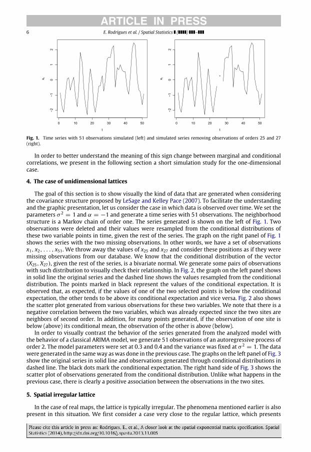
Fig. 1. Time series with 51 observations simulated (left) and simulated series removing observations of orders 25 and 27(right).

In order to better understand the meaning of this sign change between marginal and conditionalcorrelations, we present in the following section a short simulation study for the one-dimensionalcase.

4. The case of unidimensional lattices

The goal of this section is to show visually the kind of data that are generated when consideringthe covariance structure proposed by LeSage and Kelley Pace (2007). To facilitate the understandingand the graphic presentation, let us consider the case in which data is observed over time. We set theparameters σ 2

= 1 and α = −1 and generate a time series with 51 observations. The neighborhoodstructure is a Markov chain of order one. The series generated is shown on the left of Fig. 1. Twoobservations were deleted and their values were resampled from the conditional distributions ofthese two variable points in time, given the rest of the series. The graph on the right panel of Fig. 1shows the series with the two missing observations. In other words, we have a set of observationsx1, x2, . . . , x51. We throw away the values of x25 and x27 and consider these positions as if they weremissing observations from our database. We know that the conditional distribution of the vector(X25, X27), given the rest of the series, is a bivariate normal. We generate some pairs of observationswith such distribution to visually check their relationship. In Fig. 2, the graph on the left panel showsin solid line the original series and the dashed line shows the values resampled from the conditionaldistribution. The points marked in black represent the values of the conditional expectation. It isobserved that, as expected, if the values of one of the two selected points is below the conditionalexpectation, the other tends to be above its conditional expectation and vice versa. Fig. 2 also showsthe scatter plot generated from various observations for these two variables. We note that there is anegative correlation between the two variables, which was already expected since the two sites areneighbors of second order. In addition, for many points generated, if the observation of one site isbelow (above) its conditional mean, the observation of the other is above (below).

In order to visually contrast the behavior of the series generated from the analyzed model withthe behavior of a classical ARIMAmodel, we generate 51 observations of an autoregressive process oforder 2. The model parameters were set at 0.3 and 0.4 and the variance was fixed at σ 2

= 1. The datawere generated in the sameway aswas done in the previous case. The graphs on the left panel of Fig. 3show the original series in solid line and observations generated through conditional distributions indashed line. The black dots mark the conditional expectation. The right hand side of Fig. 3 shows thescatter plot of observations generated from the conditional distribution. Unlike what happens in theprevious case, there is clearly a positive association between the observations in the two sites.

5. Spatial irregular lattice

In the case of real maps, the lattice is typically irregular. The phenomena mentioned earlier is alsopresent in this situation. We first consider a case very close to the regular lattice, which presents

E. Rodrigues et al. / Spatial Statistics ( ) – 7

Fig. 2. Series generated, the dashed lines represent 20 observations generated from the conditional distributions and dotsmark the conditional expectation (left). Scatter plot of five observations generated from the conditional distribution (right).

Fig. 3. Time series generated from an autoregressive process of order 2. Dashed lines represent the 20 observations generatedfrom the conditional distributions and the points mark the conditional expectations (left). Scatter plot of 200 observationsgenerated from the conditional distribution (right).

additional counterintuitive results. In this case we observe that the change of signs occurs evenbetween first order neighbors. This situation is illustrated by the map of Iowa.

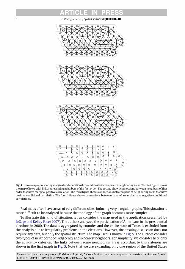
The map analyzed is shown in Fig. 4. The neighborhood criterion used was the adjacency betweenareas, i.e., two areas are considered neighbors if, and only if, they share boundaries. The neighborhoodmatrix is specified as a binary matrix, which takes only values zero and one. We fix α = −1, σ 2

= 1and hence the covariance matrix is of the form

Σα = eW′

eW,

where W is a binary matrix such that [W]ij = 1 if i and j are neighbors, and zero otherwise.We will check now for which pairs of neighbors the marginal and conditional correlations have

opposite signs. The first map in Fig. 4 shows the connections between neighbors of the first order. Thesecondmap of this same figure shows the connections between neighboring areas that havemarginalpositive correlation. Note that all pairs highlighted on the map satisfy this condition. The map on thebottom left shows connections between neighboring areas that have positive conditional correlations.Therefore, for all the connections shown in this figure there is no change of signs. The map on theright shows connections between neighboring areas that have negative conditional correlation. Thismeans that, for such linkages, sign change does occur. In this example, even first-order neighborshavemarginal and conditional correlations with opposite signs. Despite the layout closely resemblinga regular lattice, we have this additional unintuitive behavior.

8 E. Rodrigues et al. / Spatial Statistics ( ) –

Fig. 4. Iowamap representingmarginal and conditional correlations between pairs of neighboring areas. The first figure showsthe map of Iowa with links representing neighbors of the first order. The second shows connections between neighbors of firstorder that havemarginal positive correlation. The third figure shows connections between pairs of neighboring areas that havepositive conditional correlation. The fourth figure shows connections between pairs of areas that have negative conditionalcorrelations.

Real maps often have areas of very different sizes, inducing very irregular graphs. This situation ismore difficult to be analyzed because the topology of the graph becomes more complex.

To illustrate this kind of situation, let us consider the map used in the application presented byLeSage and Kelley Pace (2007). The authors analyzed the participation of Americans in the presidentialelections in 2000. The data is aggregated by counties and the entire state of Texas is excluded fromthe analysis due to irregularity problems in the elections. However, the ensuing discussion does notrequire any data, but only the spatial structure. The map used is shown in Fig. 5. The authors considertwo types of neighborhood: adjacency and k-nearest neighbors. For simplicity, we consider here onlythe adjacency criterion. The links between some neighboring areas according to this criterion areshown in the first graph in Fig. 5. Note that we are expanding only one region of the United States

E. Rodrigues et al. / Spatial Statistics ( ) – 9

Fig. 5. First-order neighbors with positive marginal correlation, with positive partial correlation and with negative partialcorrelation.

in order to facilitate visualization. The value estimated for α in the application was −0.74 and this isthe value used here. We adopted one of the D matrices used by those authors, the row-standardizedmatrix.

The second graph in Fig. 5 shows some of the pairs of neighbors that have marginal positivecorrelation. All first-order neighbors have this property. This was expected because for α < 0 allthe terms of the covariance matrix are positive. The first graph of the second line in the same figureshows the connections between first-order neighbors that have positive partial correlation. These areall neighbors of first order, i.e., in this case there is no change of sign. The last graph of this figureshows connections between first-order neighbors that have negative partial correlation, i.e., no pairof neighbors, which confirms the observation made previously. Differently from Fig. 4, we have nolinks between adjacent areas here. The reason is that Fig. 4 adopts the binary adjacency matrix for Dwhile here we use the row standardized matrix.

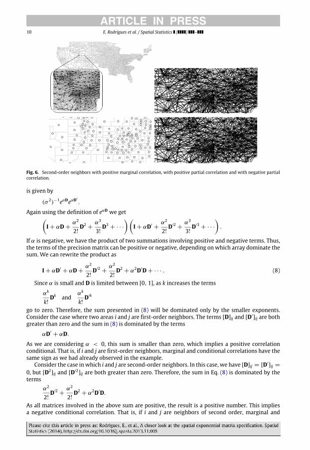
The first graph in Fig. 6 shows links between neighbors of second order. The second graph of thisfigure shows the pairs of second-order neighbors that have positive marginal correlation. As in thefirst-order neighborhood case, the correlation between any pair of areas is positive. The first graph inthe second row of Fig. 6 shows the connections between pairs of neighbors of second order that havepositive partial correlation, i.e., no pair of neighbors. The bottom right graph shows the connectionsbetween second-order neighbors that have negative partial correlation. For this kind of neighbors,there is change of signs for all pairs. This behavior is repeated in general to neighbors of even order.

The correlations for this map behave in the same way that in the regular graph. Analyzing othermaps, with completely different topological structure, with this same value for α, the same behaviorwas observed. We will see that this occurs because, as the value of α is small, the first orderneighborhood pairs dominate the covariance and precision matrices.

To understandwhy this behavior occurs for any kind ofmap, we remind that the covariancematrixof the model is given by

σ 2e−αD′

e−αD.

Ignoring the variance term σ 2 and using the definition of e−αD, this product can be written asI − αD′

+α2

2!D′2

−α3

3!D′3

+ · · ·

I − αD +

α2

2!D2

−α3

3!D3

+ · · ·

.

If α < 0, all the terms of the covariance matrix will be positive. That is, the correlation betweenany pair of areas will be positive. Let us now see what is the form of the precision matrix. This matrix

10 E. Rodrigues et al. / Spatial Statistics ( ) –

Fig. 6. Second-order neighbors with positive marginal correlation, with positive partial correlation and with negative partialcorrelation.

is given by

(σ 2)−1eαDeαD′

.

Again using the definition of eαD we getI + αD +

α2

2!D2

+α3

3!D3

+ · · ·

I + αD′

+α2

2!D′2

+α3

3!D′3

+ · · ·

.

If α is negative, we have the product of two summations involving positive and negative terms. Thus,the terms of the precisionmatrix can be positive or negative, depending on which array dominate thesum. We can rewrite the product as

I + αD′+ αD +

α2

2!D′2

+α2

2!D2

+ α2D′D + · · · . (8)

Since α is small and D is limited between [0, 1], as k increases the terms

αk

k!Dk and

αk

k!D′k

go to zero. Therefore, the sum presented in (8) will be dominated only by the smaller exponents.Consider the case where two areas i and j are first-order neighbors. The terms [D]ij and [D′

]ij are bothgreater than zero and the sum in (8) is dominated by the terms

αD′+ αD.

As we are considering α < 0, this sum is smaller than zero, which implies a positive correlationconditional. That is, if i and j are first-order neighbors, marginal and conditional correlations have thesame sign as we had already observed in the example.

Consider the case in which i and j are second-order neighbors. In this case, we have [D]ij = [D′]ij =

0, but [D2]ij and [D′2

]ij are both greater than zero. Therefore, the sum in Eq. (8) is dominated by theterms

α2

2!D′2

+α2

2!D2

+ α2D′D.

As all matrices involved in the above sum are positive, the result is a positive number. This impliesa negative conditional correlation. That is, if i and j are neighbors of second order, marginal and

E. Rodrigues et al. / Spatial Statistics ( ) – 11

Fig. 7. Correlation between first order neighbors for different values of α.

conditional correlations have opposite signs. Hence, the behavior observed in the previous exampleis not restricted to the neighborhood structure defined before. For a small value of α, whatever mapis considered, there will be change of signs in the correlations of second order neighbors.

6. How the partial correlation varies with α

The way the partial correlation varies with α also shows some non-intuitive aspects. According toLeSage and Kelley Pace (2007) the relationship between the parameter α of the proposed model andthe parameter ρ of the SAR model is given by

α ≈ ln(1 − ρ).

As the values of ρ with practical interest are ρ > 0, we observe two important points from thisrelationship. The first one is that the values of α that have practical interest are α < 0. The secondone is that α decreases as ρ increases. Taking this into consideration, it would be reasonable that themarginal and conditional correlations have a decreasing behavior with respect to the parameter α.We will see here that, for the case of conditional correlations, this is not true.

Considering again the same map used by LeSage and Kelley Pace (2007), we find the values ofthe conditional correlations for different values of the parameter α. We will check first how is thisrelationship for pairs of sites that are neighbors of first order. Fig. 7 presents the values of thecorrelations between first-order neighbors for α ranging from −1 to 0. Therefore, the conditionalcorrelation decreases with the values of α. As explained earlier, this is a reasonable behavior, becauseit means that, as the spatial association between areas becomes stronger, the conditional correlationbetween certain pairs of areas will grow. For example, α = 0 is equivalent to ρ = 0, and this meansindependence between the areas. In this case, from the graph, we see that the partial correlationbetween the neighbors of first order is zero. For α = −1 we have ρ ≈ 0.632, i.e., there should bean increase in the partial correlation between the areas. The graph presented in Fig. 7 shows that thisis what happens.

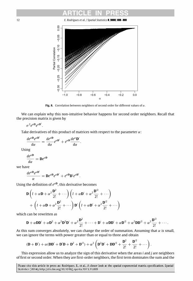
Consider now what happens to the second-order neighbors. Fig. 8 presents the values of thecorrelations between neighbors of second order for α varying in the interval [−1, 0]. The conditionalcorrelation grows with the value of α. In this case, as the value of α decreases, spatial associationbecomes stronger, the partial correlation between second-order neighbors increases, but it has anegative sign. This is not a reasonable behavior, since as the spatial association increases, it wouldbe expected that, the partial correlation between areas should increase as well, but with a positivesign and not negative, as it is observed.

12 E. Rodrigues et al. / Spatial Statistics ( ) –

Fig. 8. Correlation between neighbors of second order for different values of α.

We can explain why this non-intuitive behavior happens for second order neighbors. Recall thatthe precision matrix is given by

σ 2eαDeαD′

.

Take derivatives of this product of matrices with respect to the parameter α:

deαDeαD′

dα=

deαD

dαeαD′

+ eαD deαD′

dα.

Using

deαD

dα= DeαD

we have

deαDeαD′

α= DeαDeαD′

+ eαDD′eαD′

.

Using the definition of eαD, this derivative becomes

DI + αD + α2D

2

2!+ · · ·

I + αD′

+ α2D′2

2!+ · · ·

+

I + αD + α2D

2

2!+ · · ·

D′

I + αD′

+ α2D′2

2!+ · · ·

which can be rewritten as

D + αDD′+ αD2

+ α2D2D′+ α2D

2

2!+ · · · + D′

+ αDD′+ αD′2

+ α2DD′2+ α2D

′2

2!+ · · · .

As this sum converges absolutely, we can change the order of summation. Assuming that α is small,we can ignore the terms with power greater than or equal to three and obtain

(D + D′) + α(DD′+ D′D + D2

+ D′2) + α2D2D′

+ DD′2+

D2

2!+

D′2

2!+ · · ·

.

This expression allow us to analyze the sign of this derivative when the areas i and j are neighborsof first or second order.When they are first-order neighbors, the first term dominates the sum and the

E. Rodrigues et al. / Spatial Statistics ( ) – 13

derivative is positive. That is, the conditional correlation increases when the parameter α decreases.Remember that the conditional correlation sign has the opposite sign of each term of the precisionmatrix. Therefore, as the spatial association between the areas increases (α → −∞), the conditionalcorrelation between all neighbors of first order increases. On the other hand, if i and j are secondorder neighbors, the first term of the sum is zero and the second term is nonzero and dominatesthe sum. Since, in general, we are interested in the case where α < 0 this sum assumes a negativevalue. This means that if two areas are second-order neighbors, the conditional correlation betweenthem decreases as the parameter α decreases. That is, as the spatial association between the areasincreases, the conditional correlation between the second order neighbors gets stronger. However itgets stronger negatively, which is counterintuitive, since the increase in spatial association is leadingto conditional repulsion between the areas.

7. Conclusion

We show in this paper that the spatial model where the covariance structure depends on anexponential matrix has some important non-intuitive aspects. Despite the advantages pointed out byLeSage and Kelley Pace (2007), especiallywith regard to computational efficiency, the puzzling resultsshown here should be taken into account when considering this model. The type of non-intuitivebehavior that we found in the exponential matrix model can also be observed for other widely usedmodels, such as CAR and SARmodels. However, in the case of the lattermodels, it only occurswhen thespatial dependence parameter has a negative sign, i.e., a case with little applicability to real problems.As for the model proposed in LeSage and Kelley Pace (2007), this behavior is usually observed insituations of practical interest. Therefore, the application of this model should be done with caution,since the results may reflect a type of spatial dependence that has difficult practical interpretation.

Acknowledgment

The authors would like to thank CNPq, Capes and FAPEMIG for financial support.

References

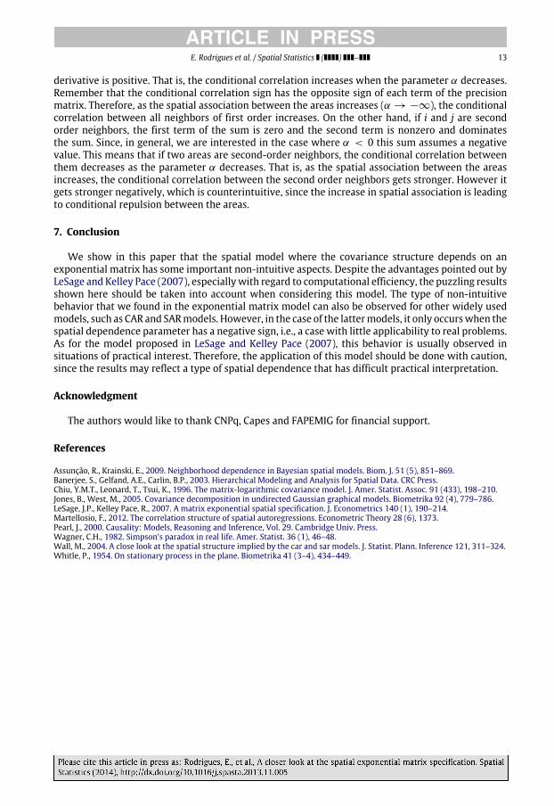
Assunção, R., Krainski, E., 2009. Neighborhood dependence in Bayesian spatial models. Biom. J. 51 (5), 851–869.Banerjee, S., Gelfand, A.E., Carlin, B.P., 2003. Hierarchical Modeling and Analysis for Spatial Data. CRC Press.Chiu, Y.M.T., Leonard, T., Tsui, K., 1996. The matrix-logarithmic covariance model. J. Amer. Statist. Assoc. 91 (433), 198–210.Jones, B., West, M., 2005. Covariance decomposition in undirected Gaussian graphical models. Biometrika 92 (4), 779–786.LeSage, J.P., Kelley Pace, R., 2007. A matrix exponential spatial specification. J. Econometrics 140 (1), 190–214.Martellosio, F., 2012. The correlation structure of spatial autoregressions. Econometric Theory 28 (6), 1373.Pearl, J., 2000. Causality: Models, Reasoning and Inference, Vol. 29. Cambridge Univ. Press.Wagner, C.H., 1982. Simpson’s paradox in real life. Amer. Statist. 36 (1), 46–48.Wall, M., 2004. A close look at the spatial structure implied by the car and sar models. J. Statist. Plann. Inference 121, 311–324.Whitle, P., 1954. On stationary process in the plane. Biometrika 41 (3–4), 434–449.