
A Classification Method of Road Transport Missions and ...
35
Received 14 June 2022, accepted 3 July 2022, date of publication 6 July 2022, date of current version 18 July 2022. Digital Object Identifier 10.1109/ACCESS.2022.3188872 A Classification Method of Road Transport Missions and Applications Using the Operating Cycle Format LUIGI ROMANO 1 , PÄR JOHANNESSON 2 , ERIK NORDSTRÖM 3 , FREDRIK BRUZELIUS 1 , RICKARD ANDERSSON 4 , AND BENGT JACOBSON 1 1 Department of Mechanics and Maritime Sciences, Chalmers University of Technology, 41296 Gothenburg, Sweden 2 RISE Research Institutes of Sweden, 41279 Gothenburg, Sweden 3 Department of Physics, Umeå University, 90187 Umeå, Sweden 4 Volvo AB, 40508 Gothenburg, Sweden Corresponding author: Luigi Romano ([email protected]) This work was supported by the Swedish Energy Agency and the Swedish Vehicle Research and Innovation Program (FFI) through the COVER Project under Grant 44929-1. ABSTRACT When dealing with customers, original equipment manufacturers (OEMs) classify vehicular usage by resorting to simplified, often colloquial, descriptions that allow for a rough understanding of the operating conditions and the user’s needs. In this way, the information retrieved from the customers is exploited to guide their choices in terms of vehicle design and configuration, based on the characteristics of the transport application, labeled using intuitive metrics. However, a common problem in this context is the absence of any formal connection to lower levels of representation that might effectively be used to assess vehicular energy performance in simulation, or for design optimization using mathematical algorithms. Indeed, both processes require more accurate modeling of the surroundings, including exhaustive information about the local road, weather, and traffic conditions. Therefore, starting with a detailed statistical description of the environment, this paper proposes a method for mathematical classification of transport missions and applications within the theoretical framework of the operating cycle (OC). The approach discussed in the paper combines a collection of statistical models structured hierarchically, called a stochastic operating cycle (sOC), with a bird’s-eye view description of the operating environment. The latter postulates the existence of different classes, which are representative of the usage and whose definition is based on simple metrics and thresholds expressed mathematically in terms of statistical measures. Algebraic expressions, called operating classes in the paper, are derived analytically for all the stochastic models presented. This establishes a connection between the two levels of representation, enabling to simulate longitudinal vehicle dynamics in virtual environments generated based on the characteristics of the intended application, using log data collected from vehicles and/or information provided by customers. Additionally, the relationships between the two descriptions are formalized using elementary probability operators, allowing for an intuitive characterization of a transport operation. An example is adduced to illustrate a possible application of the proposed method, using six sOCs parametrized from log data collected during real-world missions. The proposed approach may facilitate the interaction between OEMs, customers, and road operators, allowing for planning of maintenance, and optimization of transport missions, components, and configurations using standard procedures and routines. INDEX TERMS Autoregressive models, mission classification, operating cycle, road transport mission, stochastic modeling, stochastic operating cycle. The associate editor coordinating the review of this manuscript and approving it for publication was Chih-Yu Hsu . VOLUME 10, 2022 This work is licensed under a Creative Commons Attribution 4.0 License. For more information, see https://creativecommons.org/licenses/by/4.0/ 73087
-
Upload
khangminh22 -
Category
Documents
-
view
1 -
download
0
Transcript of A Classification Method of Road Transport Missions and ...

Received 14 June 2022, accepted 3 July 2022, date of publication 6 July 2022, date of current version 18 July 2022.
Digital Object Identifier 10.1109/ACCESS.2022.3188872
A Classification Method of Road TransportMissions and Applications Usingthe Operating Cycle FormatLUIGI ROMANO 1, PÄR JOHANNESSON 2, ERIK NORDSTRÖM 3, FREDRIK BRUZELIUS1,RICKARD ANDERSSON4, AND BENGT JACOBSON 11Department of Mechanics and Maritime Sciences, Chalmers University of Technology, 41296 Gothenburg, Sweden2RISE Research Institutes of Sweden, 41279 Gothenburg, Sweden3Department of Physics, Umeå University, 90187 Umeå, Sweden4Volvo AB, 40508 Gothenburg, Sweden
Corresponding author: Luigi Romano ([email protected])
This work was supported by the Swedish Energy Agency and the Swedish Vehicle Research and Innovation Program (FFI) through theCOVER Project under Grant 44929-1.
ABSTRACT When dealing with customers, original equipment manufacturers (OEMs) classify vehicularusage by resorting to simplified, often colloquial, descriptions that allow for a rough understanding of theoperating conditions and the user’s needs. In this way, the information retrieved from the customers isexploited to guide their choices in terms of vehicle design and configuration, based on the characteristicsof the transport application, labeled using intuitive metrics. However, a common problem in this contextis the absence of any formal connection to lower levels of representation that might effectively be usedto assess vehicular energy performance in simulation, or for design optimization using mathematicalalgorithms. Indeed, both processes require more accurate modeling of the surroundings, including exhaustiveinformation about the local road, weather, and traffic conditions. Therefore, starting with a detailed statisticaldescription of the environment, this paper proposes a method for mathematical classification of transportmissions and applications within the theoretical framework of the operating cycle (OC). The approachdiscussed in the paper combines a collection of statistical models structured hierarchically, called a stochasticoperating cycle (sOC), with a bird’s-eye view description of the operating environment. The latter postulatesthe existence of different classes, which are representative of the usage and whose definition is basedon simple metrics and thresholds expressed mathematically in terms of statistical measures. Algebraicexpressions, called operating classes in the paper, are derived analytically for all the stochastic modelspresented. This establishes a connection between the two levels of representation, enabling to simulatelongitudinal vehicle dynamics in virtual environments generated based on the characteristics of the intendedapplication, using log data collected from vehicles and/or information provided by customers. Additionally,the relationships between the two descriptions are formalized using elementary probability operators,allowing for an intuitive characterization of a transport operation. An example is adduced to illustrate apossible application of the proposed method, using six sOCs parametrized from log data collected duringreal-world missions. The proposed approach may facilitate the interaction between OEMs, customers, androad operators, allowing for planning of maintenance, and optimization of transport missions, components,and configurations using standard procedures and routines.
INDEX TERMS Autoregressive models, mission classification, operating cycle, road transport mission,stochastic modeling, stochastic operating cycle.
The associate editor coordinating the review of this manuscript and
approving it for publication was Chih-Yu Hsu .
VOLUME 10, 2022 This work is licensed under a Creative Commons Attribution 4.0 License. For more information, see https://creativecommons.org/licenses/by/4.0/ 73087

L. Romano et al.: Classification Method of Road Transport Missions and Applications Using the Operating Cycle Format
NOMENCLATURESymbol Description
C Random variable for curvature (m−1).GR Generator matrix for road type.GV Generator matrix for speed sign.Hp Random variable for precipitation occurrence.K Random variable for continuous road
curvature (m−1).Lh Mean hill length (m).Ls Sampling length for topography (m).Ltot Total road length (km).LR Mean length vector for road type (km).LRi Mean length for road type (km).LV Mean length vector for speed sign (km).LVi Mean length for speed sign (km).PH |si Conditional Markov matrix for precipitation
occurrence.PR Markov matrix for road type.PV Markov matrix for speed signs.Rt Random variable for road type.S Random variable for season.T̄ Deterministic component of air
temperature (◦C).T̃ Stochastic component of air temperature (◦C).Tair Random variable for air temperature (◦C).T ′air Modified random variable for air
temperature (◦C).T ∗air Air temperature (◦C).Td, Ty Daily and annual amplitudes of
temperature (◦C).Ts Random variable for stop time (s).V Random variable for speed sign (kmh−1).Vb Random variable for bump speed (kmh−1).Y Random variable for road grade (%).Y ′ Modified random variable for road grade (%).amaxy Lateral comfort acceleration (m s−2).eT Error term for air temperature (◦C).eY Error term for topography (%).eρ Error term for traffic density (km−1).eψ Error term for relative humidity.fHij|si Conditional number of observed transitions
for precipitation occurrence.fVij Number of observed transitions for speed
signs.gRij Entry of the generator matrix for road type.gVij Entry of the generator matrix for speed
signs.pHij|si Conditional Markov matrix entries for
precipitation occurrence.pVij Markov matrix entries for speed signs.pRij Markov matrix entries for road type.ri Road type.rturn Minimum radius of curvature (m).s season.ts Stop time (s).
tmin, tmax Minimum and maximum recommendedtime (s).
vb Bump speed (kmh−1).vi Signed speed (kmh−1).vmin, vmax Minimum and maximum recommended
speed (kmh−1).vκ Curvature speed (m s−1).y Road grade (%).9̄ Deterministic component of relative
humidity.9̃ Stochastic component of relative
humidity.9RH Random variable for relative humidity.9 ′RH Modified random variable for relative
humidity.9∗RH Relative humidity.9d, 9y Daily and annual amplitudes of relative
humidity.3p Random variable for precipitation
intensity (mmh−1).α3p|si Conditional shape parameter for
precipitation intensity.β3p|si Conditional rate parameter for
precipitation intensity (mmh−1).κ Continuous road curvature (m−1).λb Speed bump intensity (km−1).λC Curviness intensity (km−1).λp Precipitation intensity (mmh−1).λs Stop signs intensity (km−1).λRi Road type intensity (km−1).λVi Speed sign intensity (km−1).µC Modified mean curvature (lnm).µL Modified mean curve length (lnm).µT Mean temperature (◦C).µ9 Mean relative humidity.µρ Mean traffic density (km−1).πH |si Conditional stationary probability vector
for precipitation occurrence.πH1|si , πH2|si Conditional stationary probabilities for
precipitation occurrence.πR Stationary probability vector for road type.πRi Stationary probability for road type.πV Stationary probability vector for speed
signs.πVi Stationary probability for speed signs.ρ̄ Deterministic component of traffic
density (km−1).ρ̃ Stochastic component of traffic
density (km−1).ρc Critical traffic density (km−1).ρd Daily traffic density amplitude (km−1).ρt Random variable for traffic
density (km−1).ρ′t Modified random variable for traffic
density (km−1).
73088 VOLUME 10, 2022

L. Romano et al.: Classification Method of Road Transport Missions and Applications Using the Operating Cycle Format
ρ∗t Traffic density (km−1).φT |si Conditional autoregressive coefficient for air
temperature.φY Autoregressive coefficient for topography.φ9|si Conditional autoregressive coefficient for
relative humidity.φρ|si Conditional autoregressive coefficient for
traffic density.ϕTd , ϕTy Initial phases for air temperature (rad).ϕ9d , ϕ9y Initial phases for relative humidity (rad).ϕρ Initial phase for traffic density (rad).σeT |si Conditional standard deviation for the innova-
tion in the air temperature model (◦C).σeY Standard deviation for the innovation in the
topography model (%).σe9 |si Conditional standard deviation for the
innovation for the relative humidity model.σeρ |si Conditional standard deviation of the
innovation for the traffic densitymodel (km−1).
σC Modified standard deviation ofcurvature (lnm).
σL Standard deviation of curvaturelength (lnm).
σT̃ |siConditional standard deviation for thestochastic component of air temperature (◦C).
σY Standard deviation of topography (%).σ9̃|si
Conditional standard deviation for thestochastic component of relative humidity.
σρ̃|si Conditional variance for the stochasticcomponent of traffic density (km−1).
ω̄d Daily frequency (rad).ω̄y Annual frequency (rad).E(·) Exponential distribution.N (·, ·) Normal distribution.P(·) Poisson distribution.E(·) Expectation.P(·) Probability.
I. INTRODUCTIONTransport operations1 of road vehicles may differ substan-tially depending on the particular properties of the missionand the geographical area where it takes place [2]–[5]. Fromthe perspective of the intended usage, as an emblematicexample, one might compare a small, relatively low-speedtruck delivering within a municipality to a heavily loadedtimber truck traveling long distances. The characteristics ofthe operating environment also stimulate vehicles differently.
1In this paper, the notions of transport application, transport operationand transport mission are defined according to [1]. In particular, Petters-son [1] defines the transport application as the overall purpose of a vehicleduring its lifetime. This is something antecedent to the vehicle itself, andtowards which specifications should be tailored. The difference betweentransport operation and mission is less formal. The former consists of a finitenumber of tasks along a given route, the latter integrates with details fromthe surroundings. To make sense, both operation and mission assume theexistence of a vehicle, meaning that they are defined a posteriori.
Topography, number and length of curves along the road,relative wind, traffic density, and many other factors allcontribute to determining the vehicle’s behavior, impactingimportant indicators like energy efficiency and (equivalent)CO2 emissions [6]–[16].
Ideally, it would be desirable to develop individual prod-ucts for every possible route and transport mission. How-ever, due to stringent physical and economical limitations,this is impractical. Often, a viable alternative is to use astatistical approach, so that commercial vehicles are devel-oped for typical applications and geographical regions [17],[18]. Over the years, a vast scientific literature has beenproduced dealingwith the optimization of single components,configurations, or even fleets of road vehicles dependingon the intended use [19]–[27]. Specifically, many methodsproposed by researchers rely on simplified models for lon-gitudinal vehicle dynamics in combination with referencespeed profiles (called driving cycles) to simulate represen-tative operating conditions. Starting from log data, vari-ous techniques may be employed to build driving cycles,using an assortment of measures like acceleration, meanspeed and torque, cruising time, road grade, et cetera [18],[28]–[31], [31]–[53]. In particular, a first distinction maybe made between rule-based methods [54], [55] and sta-tistical ones [18], [28]–[37]. While rule-based methods arevery sensitive to the experts’ opinion and only replicate alimited number of characteristics from the measured drivingcycles [54], [55], statistical techniques correlate syntheticspeed profiles with certain operating conditions of the vehi-cle, such as cruising, idling, acceleration, or braking events.This enhanced approach combines different information(mostly inferred by speed and acceleration signals) to reflectthe characteristics of real driving scenarios [18], [28]–[37].
In turn, methods for synthesizing driving cycles basedon statistical techniques may be classified into four sub-categories: micro-trip based, segment-based, pattern classi-fication and modal cycle construction [38]. Micro-trip-basedmethods generate several candidate cycles from micro-trips.These are usually defined as excursions between consecutivestops, and may be chosen either randomly or based on spe-cific modal characteristics. Then, an optimal cycle is selectedbased on the fulfillment of some satisfaction criterion, usinga genetic algorithm [39], [40]. Driving cycles have beensynthesized with the micro-trip-based methods for the citiesof Hong Kong [41], Pune and Chennai, India, [35], [42] andSingapore [43].
In the segment-based method, a driving cycle is built frommeasured signals which are partitioned considering not onlyconsecutive stops, but also the road characteristics and trafficconditions [9]. Segments may therefore begin and end atany speed. An inherent difficulty is that constraints on speedand acceleration must be imposed in chaining the segmentstogether when synthesizing a new cycle [44], [45].
Pattern classification methods partition the speed data intokinematic sequences similar to micro-trips [31], [46]–[49].With the aid of statistical techniques, these are then classified
VOLUME 10, 2022 73089

L. Romano et al.: Classification Method of Road Transport Missions and Applications Using the Operating Cycle Format
into heterogeneous classes depending on some defined crite-ria. The final driving cycle is thus synthesized by combiningthe kinematic sequences based on the statistical propertiesof the classes. In several studies, new cycles have been con-structed from kinematics sequences using principal compo-nent analysis (PCA) and cluster analysis [56].
Finally, in the modal cycle method, the measured speeddata is clustered into snippets and classified into modal binsby using maximum likelihood estimation [31], [36], [37].A new driving cycle is then built from chosen snippetsassuming the Markov property, whose validity has alsobeen demonstrated theoretically by [49]. In particular, twoand three-dimensional Markov chains have been proposedin [36], [37]. More recently, this approach was extendedin [38] by considering variable passenger loads in the syn-thesis of driving cycles for city buses.
Further extensions to the above-referenced works on driv-ing cycles have also been presented in the literature to reflectvariation in transport operations. For example, a procedureto generate several driving cycles starting from a single busroute was proposed in [44], [45], where the investigation wasconducted concerning the number of stops [44] and variablepassenger load [45]. Both factors were shown to have a sig-nificant influence over energy consumption, which appearedto be almost normally distributed. To cope with the inherentuncertainties of driving cycles, a simulation model to predictthe energy demand of electric city buses was also developedin [57].
However, it should be emphasized that, in the process ofgeneration of driving cycles, all the information about thesurroundings is eventually lost when incorporated directlyinto a reference speed profile. From a product developmentand selection perspective, it would be preferable to use mea-sures and metrics that are independent of the vehicle, andwhich would exhaustively describe the characteristics of theenvironment. Indeed, a similar approach would make noimplicit assumption about the product. At the same time,it would allow for a more intuitive understanding of the mainphysical principles governing the longitudinal dynamics of avehicle. In this context, detailedmodeling of the surroundingsappears an essential prerequisite when tailoring the design tothe application. In the literature [1], the problem of build-ing a comprehensive mathematical model that accuratelyreplicates the driving conditions, independently of vehicleand driver, is sometimes referred to as the representationproblem.
However, as already mentioned, road vehicles are opti-mized according to the overall application and do not con-sider individual transport missions. Hence, these should begrouped and labeled based on simple scalar metrics, implyingthe need for a higher-level description. Ideally, such a repre-sentation system should condense the salient characteristicsof the usage, alongside with those of the operating envi-ronment, but without incorporating too many details aboutthe physical parameters that stimulate the vehicle’s behavior.For instance, some measures of interest would be general
statistical descriptors of the terrain, the climate, and themission itself. To adduce a concrete example, both Volvoand Scania have developed their own classification systems,namely the Global Transport Application (GTA) [2] and theUser Factor Description (UFD). Their aim is to gain an intu-itive and rough understanding of how a vehicle is operated onthe road. Using relevant feedback from maintenance shops,road operators, and ultimately customers, existing vehiclecategories are currently improved in an evolutionary man-ner. This iterative process may be further refined by usingsome modern mathematical tools. In fact, improvement andoptimization of road vehicles can certainly be addressed ina more rigorous, systematic way, provided that a suitablerepresentation of the operating environment exists. Unfor-tunately, since they were conceived to deal primarily withsatisfying the needs of customers, the GTA and UFD descrip-tions are mostly colloquial and are based on rather informalstatements. However, they may be translated in terms offrequencies and probabilities. How to systematically specifythresholds and labels to classify different missions, and howto connect these metrics with a realistic representation ofthe usage, is referred to as the classification problem in thispaper.
The last aspect connects to the variation problem. Indeed,provided that suitable metrics can be identified, even mis-sions belonging to the same transport application cannot beexpected to be identical when interpreted as individual real-izations. Ideally, it should be possible to quantify the variationwithin each category simply. This implies, however, the needfor an intermediate level of description, which should be builtaround this principle and make use of elementary statisticaltools. A similar stochastic approach tomodeling the operatingenvironment would naturally bridge the low-level descriptionconceived for representation purposes and the higher-levelclassification system discussed previously. In this context,the three levels of representation of an operating cycle (OC)respond exactly to these needs.
A. CONTRIBUTION OF THIS PAPERThus far, colloquial descriptions such as the GTA and UFDhave been exploited in an iterative process to improve exitingvehicle configurations based on the relevant feedback fromcustomers and road operators. As already mentioned, themain problem connected with this approach is that the levelof information (quantized in discrete classes) contained insuch representations is not directly usable when it comesto assessing energy performance in simulation environmentsbefore physical prototypes are built, or to optimizing vehicledesign using ad-hoc algorithms. In fact, engineers and math-ematicians need to work with more refined models of theoperating environment, which should ideally involve easilymeasurable and interpretable physical quantities.
In this context, even if the two levels of description servedifferent purposes, a formal connection between themmay beconveniently established. In this way, information collectedby customers and/or logged directly from vehicles – and
73090 VOLUME 10, 2022

L. Romano et al.: Classification Method of Road Transport Missions and Applications Using the Operating Cycle Format
hence reflecting the characteristics of the intended applica-tion – can be easily translated into a mathematical descriptionof the environment, allowing for a virtual representation thatcan be used in combination with a model for longitudinalvehicle dynamics. Such an approach would enable testingand optimization of vehicle designs and configurations basedon the user’s needs exploiting standard routines and tools.An effort in this direction has been attempted, for exam-ple, in [23], where the authors dealt with the optimizationproblem of heavy trucks for a vast combination of oper-ating conditions, including road topography modeled usingthe stochastic description proposed in this paper, in com-bination with the corresponding classes indicated by Volvo(see Section III-A1).
Therefore, the main scope of the present work is to bridgethe gap between the high and low levels of representation,enabling high-level descriptions to be used in a mathemat-ical toolchain to optimize vehicle design depending on thefeatures of the surroundings. This is done systematicallyby exploring the natural connection between a classificationsystem for road transport missions and a stochastic approachto modeling the operating environment. Specifically, theclassification and variation problems are addressed in thispaper from the perspective of the OC format [1], [58], [59].The fundamental idea is that, if the properties of the road,weather, and traffic are described using stochastic models,the same models may serve as a basis to categorize vehicularoperations based on simplified measures (the same that areused when dealing with a customer). The calculation of thismeasures may include, for instance, statistical operators likeprobability and expected value. Such simplified measureswould condense the mission and environment properties,establishing a non-bijective relationship between a certaincategory (according to some classification system), and thelower-level stochastic description. To this end, the theoreticalcontribution of this paper consists in deriving the analyticalexpressions for the above relationships, subsequently referredto as operating classes.The remainder of this paper is organized as follows.
Section II introduces the concept of an operating cycle anddiscusses the connection between its three different levelsof representation. In Section III, the analytical expressionsfor the operating classes are derived. A systematic methodof classifying individual missions and entire applications isthen proposed and illustrated in Section IV. To show how thenotion of an operating class may be used to label an operatingcycle, an example with six operating cycles, parametrizedusing measured log data from heavy trucks, is then adducedconsidering the GTA and UFD systems. The practical appli-cation of the OC format is also illustrated by comparing twodifferent vehicle configurations based on the characteristicsof the intended transport application. A discussion on thelimitations of the proposed approach, plus possible oppor-tunities for improvement, is presented in Section V. Finally,Section VI summarizes the conclusions and outlines possibledirections for future research.
II. THE OPERATING CYCLE REPRESENTATIONThe OC format is a mathematical description of a roadtransport mission that includes relevant features from thesurroundings and is independent of both vehicle and driver.Specifically, it consists of three main levels of representation,namely the bird’s-eye view, the stochastic operating cycle(sOC), and the deterministic operating cycle (dOC), arrangedin a pyramidal structure (see Figure 1). These three differentdescriptions address the classification, variation and repre-sentation problems, respectively. Each level will be describedin detail below and the relationships between the levels willbe demonstrated. A common feature of the different levelsof representation is that they all distinguish between fourfundamental categories: road, weather, traffic and mission.It is worth emphasizing that this paper builds upon theOC format, which has already been introduced in previousworks [1], [58], [59].
A. THE BIRD’s-EYE VIEWDescending the hierarchical order between the descriptions,the bird’s-eye view collocates on the top of the pyramid.It characterizes both the individual mission and the entireapplication, and uses simplified metrics and labels. It isintended to be very general, allowing for straightforwardclassification of transport operations and applications basedon a few statistical indicators [58], [60], [61]. These shouldbe ideally chosen to represent some variation in usage, perfor-mance, or properties. Themetrics and labels for the bird’s-eyeview may be defined from scratch or borrowed from existingclassification systems, as exemplified briefly for the topogra-phy parameter. In particular, the GTA system introduced byVolvo specifies four different levels [2]:
1) FLAT if slopes with a grade of less than 3% occurduring more than 98% of the driving distance.
2) P-FLAT if slopes with a grade of less than 6% occurduring more than 98% of the driving distance.
3) HILLY if slopes with a grade of less than 9% occurduring more than 98% of the driving distance.
4) V-HILLY if the other criteria are not fulfilled.
In the above example, the bird’s-eye view labels clearlycorrespond to the operating classesFLAT,P-FLAT (predom-inantly flat), HILLY and V-HILLY (very hilly), while themetrics are the values imposed on the road grade (3%, 6% and9%, respectively) and the probability of occurrence, alwaysset to 0.98. On the other hand, the User Factor Descrip-tion (UFD) used by Scania2 proposes only three classes:
1) FLAT if max 20% of the road section inclines morethan 2%.
2) HILLY if between 20-40% of the road section inclinesmore than 2%.
3) V-HILLY if more than 40% of the road section inclinesmore than 2%.
2The information on the User Factor Description (UFD) has kindly beensupplied by Scania through personal communication.
VOLUME 10, 2022 73091

L. Romano et al.: Classification Method of Road Transport Missions and Applications Using the Operating Cycle Format
FIGURE 1. Schematic representation of the pyramidal structure of an OC. All the missions being equivalent in thesense of a GTA class belong to the same transport application from the perspective of the bird’s-eye view. Theindividual statistical properties may however differ within the transport application (sOC). Finally, transport missionscan be statistically equivalent but significantly different in practice. This is captured by the dOC representation.
In both cases, the given thresholds are ambiguous, and there isno guarantee that they can reflect any significant variation inusage or performance. Furthermore, it is worth observing thatthe UFD targets single road sections, while the GTA specifiesthe different classes based on the vehicle usage, and thereforemixes the characteristics of the environment with those ofthe transport operation. One main advantage of such a vaguedescription resides in its colloquial tone. In fact, the bird’s-eyeview is the most appropriate representation when interfacingwith the customer, who cannot be expected to have a deepunderstanding of stochastic models and parameters.
Formally, the complete set of bird’s-eye view metrics maybe defined mathematically as
OCb = {Rb,Wb, Tb,Mb}, (1)
in which Rb, Wb, Tb and Wb are the sets containing allthe respective bird’s-eye view metrics in the road, weather,traffic, and mission categories. The subscript (·)b in (1) standsfor bird’s-eye view.
B. THE STOCHASTIC OPERATING CYCLEA stochastic model may be used to measure and mathemati-cally reproduce variation in a transport operation [27], [29],[32]. At the mid-level, the sOC is specifically conceived as atool to investigate the variation problem. It summarizes thestatistical properties of a transport mission and consists ofa collection of stochastic models organized hierarchically.In turn, the sOC models are provided with their own setof stochastic parameters, which are chosen to condense therelevant statistical properties (mean, variance, et cetera) ofthe corresponding physical quantity. The structure of the sOCis conceived to be as simple as possible, and the modelsare thought to be independent of each other, in obedienceto the principle of parsimony. Disregarding the correlation
between different stochastic models guarantees modularityand allows for ease of implementation and integration of newparameters, whenever required. At the same time, to bal-ance complexity and realism, a certain level of interactionbetween each model is preserved by hierarchically arrangingthe sOC itself. Parsimony is thus achieved by defining twosets of models: primary and secondary ones (subordinate).In this way, it becomes possible to build a modular structureequipped with a high level of diversification, without theneed of introducing complicated multivariate distributions.Specifically, in the sOC description, primary models for theroad and weather categories relate to the notions of road typeand season, as explained more extensively in Section III-Band Appendix A, respectively.
As with the bird’s-eye view metrics, the complete set ofsOC parameters may be defined mathematically as
OCs = {Rs,Ws, Ts,Ms}, (2)
where Rs, Ws, Ts and Ws are the sets containing all therespective sOC parameters marked as road, weather, trafficand mission. Models and parameters for the road have beenintroduced in [58], while the weather and traffic categorieshave been developed more recently in [59]. The differentstochastic models, plus their relative categories, are listed inin Table 1 and detailed later in Section III.
C. THE DETERMINISTIC OPERATING CYCLEThe dOC representation is the most adequate way of model-ing an operating cycle when it comes to individual transportmissions. It may serve as a virtual environment for realisticprediction of road vehicles’ performance, virtual testing anddesign of control algorithms, and the development of ad-hocfunctions.
73092 VOLUME 10, 2022

L. Romano et al.: Classification Method of Road Transport Missions and Applications Using the Operating Cycle Format
In the dOC, the same the physical quantities that weredeemed as models in the sOC representation3 are interpretedas parameters, and are defined as discrete functions of timeand position. Some parameters are only made dependent oneither position or time. Some others, like the ones markedin the traffic category, depend on both. Additionally, eachparameter may be represented by a scalar or a vector-valuedsignal (see dimensionality in Table 1). Any value between twodifferent discrete times (or positions) may be computed byinterpolation using the corresponding model in Table 1.To formalize the dOC format mathematically, the four
categories (see Table 1) may be defined as the sets contain-ing the parameter sequences: Rd is the set containing allsequences labeled as road,Wd for weather, Td for traffic andMd for mission. Then, the dOC format may formalized inmathematical terms as
OCd = {Rd,Wd, Td,Md}, (3)
and interpolation may be defined as an operator acting onthe elements in the sets. The dOC format provides a detailedview of individual transport operations without making anyassumptions about the driver or vehicle. Furthermore, it isbuilt in a modular fashion such that parameters may easilybe modified, added, or removed.
D. RELATIONSHIPS BETWEEN DESCRIPTIONSThe three levels of representation discussed so far are intrinsi-cally related, and ordered in a pyramidal structure, as alreadyshown in Fig. 1.The first connection which should be explored is that
between the sOC and dOC descriptions. Given a set ofstochastic parameters, a dOC may be interpreted as a singlerealization of an sOC. Indeed, by simulating its stochasticmodels, a fully parametrized sOC may be used to synthe-size multiple dOCs. Thus, these would be equivalent in astatistical sense, but might differ significantly in practice.This also implies that the map between an sOC and a dOCis not necessarily bijective; quite the opposite. Actually, thiskind of non-bijective relationship in the descending directionalso persists at the higher level between the sOC and bird’s-eye view representations. On the contrary, given a dOC, it ispossible to estimate the corresponding stochastic parametersand hence obtain an equivalent description in terms of ansOC. This is usually done by resorting to elementary statisti-cal methods, and assuming plausible probability distributionsand stochastic models.
On the other hand, the bird’s-eye view and the sOC areboth statistical descriptions, but with considerably differ-ent resolutions. Indeed, while the bird’s-eye view generallyencompasses an entire transport application (but might alsobe used to classify single operations and even road sections),the sOC only targets individual missions. The formal relation-ship between the two levels may be elucidated by looking
3The relationship between the role of a physical quantity in the sOC anddOC representations is perhaps better understood from Table 1, where eachentity is labeled under model for the sOC and parameter for the dOC.
at the GTA classes previously introduced. Again, using thetopography as an example, it is possible to estimate theprocess variances which yield the thresholds set by the GTAclassification system, i.e. the bird’s-eye viewmetrics (as donein Section III-A). Thus, given an sOC, the correspondingGTA class may always be deduced uniquely. The inverseoperation is not possible since, for a predetermined GTAclass, infinitely many sOCs may exist. More specifically,the authors of this paper are concerned with showing that,for a generic model ξ in the road, weather, and traffic OCcategories, the elements in the set of sOC parameters OCsand the bird’s-eye view metrics in the setOCb may be relatedas follows:
aξ(ηb,ξ
)< gξ
(ηs,ξ , ηb,ξ
)≤ bξ
(ηb,ξ
), (4)
where ξ ∈ XR,XW orXT is a generic sOCmodel,XR,XW ,and XT denote the sets of sOC models for the road, weather,and traffic categories, respectively, ηs,ξ ∈ Rs,ξ , Ws,ξ , Ts,ξand ηb,ξ ∈ Rb,ξ , Wb,ξ , Tb,ξ are vectors of sOC parametersand bird’s-eye-view metrics for the model ξ , Rs,ξ ⊂ Rs,Ws,ξ ⊂ Ws, Ts,ξ ⊂ Ts are subsets of sOC parameters forthe model ξ , and Rb,ξ ⊂ Rb, Wb,ξ ⊂ Wb, Tb,ξ ⊂ Tb aresubset of bird’s-eye-view metrics for the model ξ .
Finally, aξ (ηb,ξ ) and bξ (ηb,ξ ) represent lower and upperbounds for the vector-valued function gξ (·, ·) appearing in (4).In this context, it should be clarified that the inequalities (4)need to be interpreted element-wise. Basically, they postulatethe existence of certain relationships which mathematicallyformalize the so-called operating classes. It may be inferredfrom (4) that, for each model in each category, the corre-sponding operating class depends solely on the sOC param-eters used to describe that model, plus the correspondingbird’s-eye view metrics.
The analytical derivation of the relationships for the oper-ating classes is carried out in Section III.
III. DERIVATION OF THE OPERATING CLASSESThe main analytical contribution of this paper lies in thederivation of the aforementioned operating classes.
In the remainder of the paper, the notation is as follows:for a generic random variable A : �A 7→ SA, its realizationsare denoted by a, unless specified otherwise. For continuousand discrete random variables, respectively, probability den-sity functions (PDFs) and probability mass functions (PMFs)are denoted by fA(·) and pA(·), and their argument oftenby a. Cumulative distribution functions (CDFs) are writtenas FA(·). For a generic function written as f (·; ·), the semi-colon is used to separate variables from parameters. Multiplevariables or parameters may be additionally separated usingcommas. The set of real numbers is denoted by R; the sets ofpositive and negative real numbers are denoted by R≥0, R≤0when including the zero and by R>0, R<0 when excluding it.The set of positive integer numbers is denoted by N, whereasN0 denotes the extended set of positive integers includingzero, i.e. N0 = N ∪ {0}. Sequences of random variables aredenoted by {Ak}k (the subscript k is often dropped when the
VOLUME 10, 2022 73093

L. Romano et al.: Classification Method of Road Transport Missions and Applications Using the Operating Cycle Format
TABLE 1. Stochastic models and deterministic parameters (dOC parameters) for the sOC and dOC representations. Linear and constant refer to linear andright-side continuous piecewise constant interpolation models respectively. The mathematical model of Dirac delta occurs when the parameter isregarded as an isolated event.
clarity allows). Indicator functions are denoted by 1a∈A andassume a value of one if a ∈ A and zero otherwise.
A. ROAD CATEGORYIn the sOC description, the road category comprises stochas-tic models for topography, curviness, speed bumps, stopsigns, road roughness, speed signs, and ground type. The cor-responding operating classes are derived in the following, andconnect the sOC parameters to the bird’s-eye view metrics.
It is worth mentioning that all the road models presentedin this paper have been chosen as a compromise betweensimplicity and accuracy, in obedience to the already men-tioned principle of parsimony. In particular, the models fortopography, curviness and road roughness are based on theextensive research presented in [10], [11], [62]–[67]. Simi-larly, the models for speed bumps, stop and speed signs, androad and ground types were introduced and validated in [58].
1) TOPOGRAPHYTopography plays a major role in determining the overallenergy performance of road vehicles. Indeed, positive roadgrades are responsible for resistive forces that oppose longitu-dinal motion, resulting in increased energy consumption [19].Negative road grades, in contrast, produce forces that accel-erate the vehicle downhill, and may considerably impact thelife and performance of the mechanical components of thebraking system. Negative slopes are also exploited by battery
electric vehicles (BEVs) for regenerative braking [23]. Owingto these premises, it should not be surprising that both Volvoand Scania include the topography parameter in their classi-fication systems.
In the sOC, the road is partitioned into k ∈ N short seg-ments of fixed length Ls, and the grade {Yk}k∈N is regarded asa randomvariable on each of them. Specifically, it is restrictedto assuming values between a minimum and maximum:
Yk = min(max
(−yc,Y ′k
), yc), (5)
where yc ∈ R>0 is an imposed limit on the maximum roadgrade expressed as a percentage. By default, it may be setto yc = 100. The modified topography Y ′k is then modeledusing a stationary, first-order autoregressive AR(1) processas follows [10], [11]:
Y ′k = φYY′
k−1 + eY ,k , eY ,k ∼ N(0, σ 2
eY
), (6)
where φY ∈ (−1, 1) and σeY ∈ (0,∞) are the two character-istic parameters. According to (6), the modified road gradeitself is normally distributed [68], i.e.
Y ′ ∼ N(0, σ 2
Y
), (7)
where the subscript k has been omitted for ease of notation.The process variance σ 2
Y reads
σ 2Y =
σ 2eY
1− φ2Y. (8)
73094 VOLUME 10, 2022

L. Romano et al.: Classification Method of Road Transport Missions and Applications Using the Operating Cycle Format
Furthermore, the autoregressive coefficient φY may be alsorewritten as a function of the hill length Lh:
φY = sin(π
2− 2
LsLh
), (9)
where Ls is the sampling length.Thus, the model for the topography may be equivalently
parametrized using the hill length Lh and the standard devi-ation σY defined in (8) and (9), which are easier to interpretthan φY and σeY . Therefore, the set of stochastic road param-eters relating to the topography model may be formalized asRs,Y = {Lh, σY }.Following the interpretation of the GTA and UFD classi-
fications, the operating class for the topography connectingthe sOC and bird’s-eye view representations may be derivedby considering the probability that the road grade comprisesa value between a minimum and a maximum. This value ofprobabilitymay range between lower and upper bounds py,minand py,max, respectively. In formula: py,min < P(ymin < |Y | ≤ymax) ≤ py,max. The corresponding formula for the operatingclass is then given in Result 1.Result 1 (Operating Class for Topography): For the road
topography model described by (5)-(9), the following expres-sion for the operating class may be deduced:
py,min < 1ymax∈[yc,∞) +
[28(ymax
σY
)− 1
]1ymax∈[0,yc)
−
[28(ymin
σY
)− 1
]1ymin∈[0,yc)
−1ymin∈[yc,∞) ≤ py,max, (10)
where the function 8(·) is the CDF of the standard normaldistribution.
Proof: Noticing that
P (|Y | ≤ y) = FY (y; σY , yc)
= P(∣∣Y ′∣∣ ≤ y)1y∈[0,yc) + 1y∈[yc,∞), (11)
and recalling that
P(∣∣Y ′∣∣ ≤ y) = FY ′ (y; σY )− FY ′ (−y; σY )
= 28(yσY
)− 1 (12)
immediately yields (10).It may be observed that (10), despite being scalar, has
the same structure of (4), and connects the elements in theset of sOC parameters for topography Rs,Y = {Lh, σY }with the bird’s-eye view metrics in the set Rb,Y =
{ymin, ymax, py,min, py,max}.The above inequality (10) may be solved numerically
for σY , once the bird’s-eye view metrics have been speci-fied. Again, adducing the example of the GTA classificationsystem, the four different values ymin = 0, ymax = 3, 6and 9 prescribed for the road grade in (10) as a percentageof the road length and the limits py,min = 0.98, py,max = 1yield the values of σY reported in Table 2 for the classes
TABLE 2. Topography classes according to the GTA and UFD classificationsystems with the corresponding intervals for the standard deviation σY .
FLAT, P-FLAT, HILLY and V-HILLY. On the other hand,as already mentioned, the UFD misses the P-FLAT class.Indeed, it only specifies one limit ymax = 2 (ymin is alwayszero) for the road grade in (10), and two different probabilitythresholds py,max = 0.2 and 0.4, respectively. The ranges forthe standard deviation σY corresponding to each topographyclass are listed in Table 2 for both classification systems.
It should be noted that, according to both theGTA andUFDsystems, in the bird’s-eye view description the hill length Lhis not included in the determination of the specific operatingclass. Thus, according to the bird’s eye view representation,road segments with the same process variance σ 2
Y but differenthill lengths Lh are formally equivalent. A possible extensionto the original definition for the operating class would be toalso take into account the hill length Lh, by postulating anadditional relationship of the form:
Lh,min < Lh ≤ Lh,max. (13)
Together, (10) and (13) would more accurately characterizethe road topography. Also in this case, (10) and (13) havethe same form of (4), connecting the elements in the setRs,Y = {Lh, σY } with the bird’s-eye view metrics in Rb,Y =
{ymin, ymax, py,min, py,max,Lh,min,Lh,max}.As an example, a comparison between measured data from
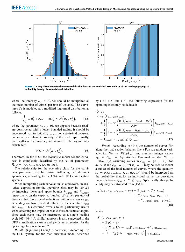
a log file (corresponding to sOC 2 in Section IV-C) and theanalytical PDF and CDF for the road topography accordingto Eqs. (11) and (12) is shown in Fig. 2.
2) CURVINESSLateral acceleration due to curves along the road typicallyinduces the driver to decelerate, resulting in increased energyconsumption. In this context, two main contributing phenom-ena may be identified: the reduced efficiency of the primemover and the losses due to pure or combined slip condi-tions that take place inside the tire contact patches [69]–[71].Moreover, lateral load due to road curvature has a substantialimpact on the fatigue of the mechanical components of avehicle, reducing their useful life [62]–[64]. Therefore, thecurviness parameter is accounted for in both Volvo’s andScania’s descriptions.
In the sOC, a curve is regarded as an independent eventhaving a location, curvature (inverted radius), and length.This description – referred to as the curviness of the road –was adapted in [58] from [62] and is denoted in this paper bythe sequence {Xk ,Ck ,Lk}k∈N. Specifically, the locations aremodeled using a Poisson process, i.e.
Xk+1 − Xk ∼ E(λC ), (14)
VOLUME 10, 2022 73095
L. Romano et al.: Classification Method of Road Transport Missions and Applications Using the Operating Cycle Format
FIGURE 2. Comparison between the measured distribution and the analytical PDF and CDF of the road topography: (a)probability density; (b) cumulative distribution.
where the intensity λC ∈ (0,∞) should be interpreted asthe mean number of curves per unit of distance. The curva-tures Ck is modeled as a modified lognormal distribution asfollows:
1Ck= R′k + rturn, lnR′k ∼ N
(µC , σ
2C
), (15)
where the parameter rturn ∈ (0,∞) appears because roadsare constructed with a lower bounded radius. It should beunderstood that, technically, rturn is not a statistical measure,but rather an inherent property of the road type. Finally,the lengths of the curve Lk are assumed to be lognormallydistributed:
lnLk ∼ N(µL , σ
2L
). (16)
Therefore, in the sOC, the stochastic model for the curvi-ness is completely described by the set of parametersRs,C = {λC , rturn, µC , σC , µL , σL}.The relationship for the operating class for the curvi-
ness parameter may be derived following two differentapproaches, according to the GTA and UFD classificationsystems.
When interpreting each curve as an isolated event, an ana-lytical expression for the operating class may be derivedby imposing lower and upper bounds n̄′C,min and n̄′C,max,respectively, on the expected number of curves per unit ofdistance that force speed reductions within a given range,depending on two specified values for the curvature κminand κmax. This criterion reveals to be particularly usefulwhen assessing the impact of road curves on vehicle fatigue,since each event may be interpreted as a single loadingcycle [63], [64]. A similar approach is also suggested in theUFD classification system and yields an expression for theoperating class as in Result 2.Result 2 (Operating Class for Curviness): According to
the UFD system, for the road curviness model described
by (14), (15) and (16), the following expression for theoperating class may be deduced:
n̄′C,min
< λC(1κmax∈[1/rturn,∞)
+12
[1− erf
(ln(1/κmax − rturn)− µC
√2σC
)]1κmax∈(0,1/rturn)
−12
[1− erf
(ln(1/κmin − rturn)− µC
√2σC
)]1κmin∈(0,1/rturn)
− 1κmin∈[1/rturn,∞))≤ n̄′C,max. (17)
Proof: According to (14), the number of curves NCalong the road section behaves like a Poisson random vari-able, i.e. NC ∼ P(λCLtot), and assumes integer valuesnC ∈ SNC ≡ N0. Another Binomial variable N ′C ∼Bin(NC , pκ ), assuming values in SN ′C = {0, . . . , nC } fornC > 0 and SN ′C = {0} for nC = 0, may be used to modela subset of the total number of curves, where the quantitypκ = pκ (κmin, κmax, rturn, µC , σC ) should be interpreted asthe probability that, for an individual curve, the curvatureranges between κmin < C ≤ κmax. Specifically, this prob-ability may be estimated from (15) as
pκ (κmin, κmax, rturn, µC , σC ) = P(κmin < C ≤ κmax
)= FC (κmax; rturn, µC , σC )
−FC (κmin; rturn, µC , σC ),
(18)
where
FC (κ; rturn, µC , σC )
= P (C ≤ κ)= P
(R′ ≥ 1/κ − rturn
)1κ∈(0,1/rturn) + 1κ∈[1/rturn,∞)
=
[1− FR′
(1/κ − rturn;µC , σC
)]1κ∈(0,1/rturn)
73096 VOLUME 10, 2022

L. Romano et al.: Classification Method of Road Transport Missions and Applications Using the Operating Cycle Format
+1κ∈[1/rturn,∞)
=12
[1− erf
(ln(1/κ − rturn)− µC
√2σC
)]1κ∈(0,1/rturn)
+1κ∈[1/rturn,∞). (19)
From the law of total expectation, it also follows that
E(N ′CLtot
)=
1Ltot
E(E(N ′C
∣∣ NC)) = 1Ltot
E(NCpκ )
= λCpκ (κmin, κmax, rturn, µC , σC ). (20)
Combining (18), (19) and (20) gives the result.The operating class (17) connects the set of sOC parame-
ters Rs,C = {λC , rturn, µC , σC , µL , σL} with that of bird’s-eye view metrics Rb,C = {κmin, κmax, n̄′C,min, n̄
′C,max}.
It should be observed that µL and σL do not appear in (17),since the curves along the road are regarded as isolated events.
On the other hand, the GTA description regards the cur-vature κ(x) as a function of the position along the road.In this context, the road section may be classified in respectto the curviness calculating the probability that the curvature,treated as a random variable K , assumes values between κminand κmax, and specifying two limits pκ,min and pκ,max. Thiswould be equivalent to consider a relationship of the formpκ,min < P(κmin < K ≤ κmax) ≤ pκ,max. In particu-lar, the probabilities pκ,min and pκ,max should be interpretedas the minimum and maximum ratios between the portion ofthe road for which κmin < K ≤ κmax and the total lengthof the segment, denoted by Ltot. In this case, an approxi-mated expression for the operating class may be derived asin Result 3.Result 3 (Operating Class for Curviness): According to
the GTA system, for the road curviness model describedby (14), (15) and (16), the following expression for theoperating class may be deduced:
pκ,min <
[1− λC exp
(µL +
σ 2L
2
)]×
(1κmax∈[0,1/rturn) − 1κmin∈[0,1/rturn)
)+1κmax∈(0,1/rturn)
λC
2exp
(µL +
σ 2L
2
)×
[1− erf
(ln(1/κmax − rturn)− µC
√2σC
)]−1κmin∈(0,1/rturn)
λC
2exp
(µL +
σ 2L
2
)×
[1− erf
(ln(1/κmin − rturn)− µC
√2σC
)]+1κmax∈[1/rturn,∞)−1κmin∈[1/rturn,∞)≤pκ,max. (21)
Proof: To derive (21), it is worth observing that positionalong the road may be described by a random variable X ,assuming values x ∈ SX = [0,Ltot]. The space SX maybe divided into two subsets K and K̄, corresponding to therespective portions for which the road curvature is equal toor different from zero. Clearly, SX = K ∪ K̄. Owing to
these premises, a continuous function K (X ) of the randompositionX along the roadmay be constructed starting with themodel for the curviness discussed in [58], whereas this paperproposes a simplified approach. In particular, the curvatureKis approximated as a piecewise continuous function of X , andthe effect of superimposing curves is disregarded. Therefore,the total probability P(κmin < K ≤ κmax) may be calculatedstarting from the relationship
P(K ≤ κ) = P(K ≤ κ | X = x ∈ K̄
)P(X = x ∈ K̄
)+ P
(C ≤ κ | X = x ∈ K
)P(X = x ∈ K)
=[1− P(X = x ∈ K)
]1κ∈[0,1/rturn)
+ P(C ≤ κ | X = x ∈ K
)× P(X = x ∈ K)1κ∈(0,1/rturn)+1κ∈[1/rturn,∞), (22)
where P(C ≤ κ | X = x ∈ K) reads as in (19) andthe probability P(X = x ∈ K) may be approximated usingWald’s equation as
P(X = x ∈ K) ≈ E
(1Ltot
NC∑k=1
Lk
)=
1Ltot
E(NC )E(L1)
= λC exp(µL +
σ 2L
2
). (23)
In the derivation of (23), it is worth emphasizing that, accord-ing to (14) and (16), the random variable NC is, by construc-tion, independent of the sequence of curve lengths {Lk}k∈N.Combining (18), (22) and (23) yields the desired result.
The relationship (21) is the expression for the oper-ating class relating the curviness parameters Rs,C =
{λC , rturn, µC , σC , µL , σL} of the sOC and the bird’s-eyeview metrics Rb,C = {κmin, κmax, pκ,min, pκ,max} (accordingto the GTA representation).
Comparing (17) and (21), the classification criterion pro-posed by the GTA system appears more refined than that ofthe UFD description, since it also accounts for the length ofthe curves via the parameters µL and σL .
Figure 3 compares the analytical expression (22) forthe CDF of the road curviness against the distributionextracted from the original log file corresponding to sOC 2in Section IV-C.
3) SPEED BUMPS AND STOP SIGNSIn the UFD, another criterion used to classify a transport mis-sion relates to the obstacle height of the speed bumps that maybe found along the vehicle’s trajectory. These force the driverto reduce their cruising speed, often resulting in increasedenergy consumption. A similar effect is produced by thestop signs, which clearly impose a driving speed of zero.Speed bumps and stop signs are modeled similarly in the sOCrepresentation. They are regarded as independent events anddescribed by the sequences {Xk ,Vb,k}k∈N and {Xk ,Ts,k}k∈N,respectively, whereXk is again the location,Vb,k is interpretedas a recommended speed, and Ts,k as a recommended time.
VOLUME 10, 2022 73097

L. Romano et al.: Classification Method of Road Transport Missions and Applications Using the Operating Cycle Format
FIGURE 3. Comparison between the measured cumulative distributionand the analytical CDF obtained from the curviness model.
The distance between two consecutive events is assumed tobe exponentially distributed, as in (14), but with intensitiesλb and λs. The recommended speed Vb,k and time Ts,k aresupposed to be uniformly distributed between aminimum andmaximum value, i.e.
Vb,k ∼ U(vmin, vmax
), (24a)
Ts,k ∼ U(tmin, tmax
). (24b)
Analogous to what done for the curviness, the road sectionmay be characterized by imposing a limit on the expectednumber of speed bumps or stops that cause considerablespeed reductions or prescribe sufficiently long standstilltimes. A similar approach is proposed in the UFD for roadobstacles, whereas the GTA classification system makes noreference to either speed bumps or stop signs. Starting withthe model for speed bumps, the operating class may be for-malized mathematically as in Result 4.Result 4 (Operating Class for Speed Bumps): For the spe-
ed bumps model described by (24a), the following expressionfor the operating class may be deduced:
n̄′b,min < λb
[1vb,max∈[vmax,∞) − 1vb,min∈[vmax,∞)
+
(vb,max − vmin
vmax − vmin
)1vb,max∈(vmin,vmax)
−
(vb,min − vmin
vmax − vmin
)1vb,min∈(vmin,vmax)
]≤ n̄′b,max.
(25)
Proof: The number of events per unit of length maybe described again using a Poisson random variable, Nb ∼
P(λbLtot), assuming integer values nb ∈ SNb ≡ N0. TheBinomial variable N ′b ∼ Bin(Nb, pb) may instead be intro-duced to model the number of speed bumps that imposesevere speed reductions or long standstill times. It wouldassume integer values in the space SN ′b = {0, . . . , nb} fornb > 0 and SN ′b = {0} for nb = 0. The quantity pb representsthe probability that the recommended speed Vb is lower thana specified threshold, and may be computed from (24a) as
pb (vb,min, vb,max, vmin, vmax)
, P(vb,min < Vb ≤ vb,max)
= FVb (vb,max; vmin, vmax)− FVb (vb,min; vmin, vmax)
= 1vb,max∈[vmax,∞) +
(vb,max − vmin
vmax − vmin
)1vb,max∈(vmin,vmax)
−
(vb,min − vmin
vmax − vmin
)1vb,min∈(vmin,vmax) − 1vb,min∈[vmax,∞).
(26)
Calculating E(N ′b/Ltot) as in (20) and specifying lower andupper bounds n̄′b,min, n̄
′
b,max on the expected number of speedbumps per unit of distance yields the result.
The expression (25) establishes a relationship between thesOC parameters Rs,Vb = {λb, vmin, vmax} and the bird’s-eyeviewmetricsRb,Vb = {vb, n̄
′
b,min, n̄′
b,max}. The correspondingrelationship for stop signs may be derived with the samerationale:
n̄′s,min < λs
[1ts,max∈[tmax,∞) − 1ts,min∈[tmax,∞)
+
(ts,max − tmin
tmax − tmin
)1ts,max∈(tmin,tmax)
−
(ts,min − tmin
tmax − tmin
)1ts,min∈(tmin,tmax)
]≤ n̄′s,max. (27)
4) ROAD ROUGHNESSRoad roughness plays an important role when it comes todurability and fatigue of mechanical components, but has aminor impact on energy efficiency. Nonetheless, this param-eter is included in both the GTA and UFD systems.
Road profiles are traditionally modeled using Gaussianprocesses [72]. This choice works satisfactorily for smallsections of roads, whereas variability between sections maybe better explained using generalized Laplace models. Thesemay be interpreted as Gaussian processes with randomlyvarying variance. In the sOC representation, the model for theroad profile Z (x) is based on the definition given by the ISOstandard 8608 [73], which uses a two-parameter spectrum:
SZ (�) = Cr
(�
�0
)−w, �1 ≤ � ≤ �2, (28)
and zero otherwise. In (28),� is the spatial angular frequency,�0 = 1, �1 = 2π · 0.011, �2 = 2π · 2.83 [73] are twocut frequencies expressed in radians per metre, and Cr is thedegree of unevenness, also called the roughness coefficient.Finally, the waviness parameter w is assumed to be constantand set tow = 2. The sOC description employs a Laplace ISOmodel [10], [11], [65], [66], parametrized by its mean rough-ness Cr and the Laplace shape parameter νr (or, equivalently,its variance and kurtosis).
Taking inspiration from the ISO classification [73], theroad may be labeled in respect to the roughness dependingon the degree of unevenness Cr:
Cr,min < Cr ≤ Cr,max. (29)
In particular, the ISO standard [73] specifies eight differentroad levels, ranging from class A to H in increasing roughness
73098 VOLUME 10, 2022

L. Romano et al.: Classification Method of Road Transport Missions and Applications Using the Operating Cycle Format
order. Amongst these, however, only the first five are impor-tant for automotive applications [74]. A similar criterion isadopted in this paper to the sOC description. Accordingly,only (29) is required to establish a relationship between theset of sOC parameters Rs,Z = {Cr, νr} and the two limitsin the set Rb,Z = {Cr,min,Cr,max}. It should be noted thatthe proposed criterion systematically neglects the effect ofvariability between sections, since the shape parameter νrdoes not appear in (29). By contrast, a more refined classi-fication approach would prescribe an additional relationshipincluding νr. To this end, further details on generalizedLaplace distributions may be found in [67], [75].
5) SPEED SIGNS AND GROUND TYPEThe legal speed dramatically impacts the energy performanceof road vehicles. In fact, while constant cruising speeds maybe observed to be apparently optimal from an energy effi-ciency perspective, frequent variations in driving speed resultin increased consumption [23].
On the other hand, the ground type and the asphalt prop-erties play an important role in determining the maximumtraction forces that the tires can generate, and have alsoa substantial effect on rolling resistance [76]–[79]. Thesetwo aspects are particularly significant for electric vehicles,in connection to both the higher instantaneous torques thatthe wheels may experience and the well-known phenomenonof range anxiety.
Accordingly, both theGTA andUFD classification systemsinclude the above-mentioned parameters.
In the sOC description, speed signs and ground type behaveas piecewise constant, right-side continuous functions of theposition [58]. Since the same stochasticmodel is used for bothentities, only the speed signs are discussed. Specifically, theseare treated as a random process V = V (x) along with theposition x ∈ R on the road. The variable V (x) is only allowedto take discrete values in the state space SV = {v1, . . . , vnv},where nv denotes the finite number of possible speed limits.The entire process is then split into two parts and modeled asa sequence of positions, with the locations of the signs, andspeeds {Xk ,Vk}k∈N.It is also assumed that the current speed limit exerts the
greater part of the influence on the upcoming limit. Thus, forthe sake of simplicity, the sequence of speed limits is modeledas a Markov chain [80], [81]:
P(Vk+1 = vi,k+1
∣∣V1 = vi,1,V2 = vi,2, . . . ,Vk = vi,k)
= P(Vk+1 = vi,k+1
∣∣Vk = vi,k), (30)
where the generic signed speed vi is an element of the speedvector v = [v1 . . . vnv ]
T.The Markov probability matrix PV ∈ Rnv×nv
≥0 fully char-acterizes the chain. An entry pVij models the conditionalprobability of transitioning from state i to state j and satisfies∑nv
j=1 pVij = 1. The description may be reduced further byobserving that the speed limit model is embedded in thatof the locations and that there are no self-transitions, so all
diagonal elements are equal to zero, i.e. pVii = 0. Instead, theoff-diagonal elements may be easily estimated from data bymeasuring the number of changes fVij between states i and j.Moreover, in the modeling of the road type sequence, it isassumed that there are no absorbing states. The speed signlocations may be modeled as in (14). However, each stateis expected to have its own intensity: nv states introduce nvparameters λV1, . . . , λVnv , which may be deduced from themean length LVi of speed limit vi:
λVi =1LVi. (31)
As for the speed, the nv mean lengths LVi may be organizedinto a vector LV = [LV1 . . . LVnv ]
T. Thus, the completedescription consists of the conditional probabilities pVij andthe nv mean lengths LVi (or, alternatively, the intensities λVi).Furthermore, the fact that the distance Xk+1 − Xk betweenconsecutive positions is exponentially distributed implies thatV (x) itself becomes a continuous-time4 Markov chain [80].In particular, the stationary distribution πV of the overallprocess may be derived starting from the knowledge of thegenerator matrix GV , and satisfies the equation
πVGV = 0, (32)
where the entries gVij = gVij(pVij,LVi) of GV are given by
gVij(pVij,LVi
)=
λVipVij =
pVijLVi
, i 6= j,
−λVi = −1LVi, i = j.
(33)
Form a bird’s-eye view perspective, the operating classmay be defined by considering the probability that the speedover the road section ranges between a minimum v̂min and amaximum v̂max. This probability value may be constrainedbetween lower and upper bounds pv,min and pv,max, i.e.pv,min < P(v̂min < V ≤ v̂max) ≤ pv,max. This criterionis similar to that used in the UFD representation system.Denoting by I(v̂min,v̂max] the set comprising the values of isuch that vi ∈ (v̂min, v̂max], the relationship connecting thesOC parameters Rs,V = {v,PV ,LV } to the bird’s-eye viewmetrics Rb,V = {v̂min, v̂max, pv,min, pv,max} may be found inthe form
pv,min <∑
i∈I(v̂min,v̂max]
πVi(PV ,LV ) ≤ pv,max, (34)
subjected to the constraint∑nv
i=1 πVi = 1.Instead, the GTA description proposes that a transport
mission should be classified based on the expected numberof transitions between speeds along the road, per unit oflength. To formalize this mathematically, the variable NfV ,assuming values in SNfV ≡ N0, is introduced to modelthe number of speed changes occurring on a road of total
4Continuous Markov chains are traditionally called continuous-timeMarkov chains, even though, in the present case, the dimension being con-sidered is space rather than time.
VOLUME 10, 2022 73099

L. Romano et al.: Classification Method of Road Transport Missions and Applications Using the Operating Cycle Format
length Ltot. This criterion may be integrated with informationabout the mean legal speed along the road, thus imposing alsov̂min < E(V ) ≤ v̂max. The two conditions yield the set ofanalytical expressions for the operating class as in Result 5Result 5 (Operating Class for Speed Signs): According to
the GTA system, for the speed signs model describedby (30)-(33), the following expressions for the operating classmay be deduced:
n̄fV ,min <1Ltot
∞∑nfV =0
nv∑j=1
nv∑i=1
nfV p̂ij(nfV ;Ltot
)×πVi(PV ,LV ) ≤ n̄fV ,max, (35a)
v̂min <
nv∑i=1
viπVi(PV ,LV ) ≤ v̂max. (35b)
Proof: The probability p̂ij(nfV ;Ltot) , P(NfV = nfV ∩V (Ltot) = vj | V (0) = vi) of having exactly nfV > 0 numberof transitions when V (Ltot) = vj conditioned to V (0) = vimay be calculated as [82], [83]
p̂ij(nfV ;Ltot
)=
∑k 6=i
∫ Ltot
0egVii(pVij,LVi)(Ltot−L)
× gVik(pVij,LVi
)p̂kj(nfV − 1;L
)dL, (36)
with initial condition p̂ij(0;Ltot) = pVijegii(pVij,LVi)Ltot [83].Supposing that the initial probability of being in the statevi coincides with the stationary one, the total probabilityp̂j(nfV ;Ltot) , P(NfV = nfV ∩V (Ltot) = vj) of having exactlynfV transitions when V (Ltot) = vj then becomes
p̂j(nfV ;Ltot
)=
nv∑i=1
P(NfV = nfV ∩ V (Ltot) = vj
∣∣ V (0) = vi)
×πVi(PV ,LV )
=
nv∑i=1
p̂ij(nfV ;Ltot
)πVi(PV ,LV ). (37)
Summing over j yields the probability of having exactly nfVspeed jumps along a road of length Ltot, i.e. the PMF
pNfV(nfV ; pVij,LV ,Ltot
)=
nv∑j=1
p̂j(nfV ;Ltot
)=
nv∑j=1
nv∑i=1
p̂ij(nfV ;Ltot
)πVi(PV ,LV ). (38)
Accordingly, the expected value of speed transitions per unitof length E(NfV /Ltot) reads
E(NfVLtot
)=
1Ltot
∞∑nfV =0
nfV pNfV(nfV ;PV ,LV ,Ltot
)=
1Ltot
∞∑nfV =0
nv∑j=1
nv∑i=1
nfV p̂ij(nfV ;Ltot
)
TABLE 3. Probabilities psi for each season assuming that the year isalways composed of 365 days.
×πVi(PV ,LV ), (39)
which gives (35a). The derivation of (35b) is trivial and henceomitted.The inequalities (35) relate the set of sOC parameters
Rs,V = {v,PV ,LV } with that of bird’s-eye view metrics,denoted by Rb,V = {v̂min, v̂max, n̄fV ,min, n̄fV ,max}. It may beobserved that (39) yields a rather complicated expression forthe total number of transitions per unit of length. A simplerapproach would be to approximate the number of transitionsto the state i considering the asymptotic or limiting distribu-tion, i.e. E(NfV /Ltot) ≈
∑nvi=1 πVi/LVi, so that (35a) becomes
n̄fV ,min <
nv∑i=1
πVi(PV ,LV )LVi
≤ n̄fV ,max. (40)
The above relationship (40) may be used in place of (35a) toestablish a formal expression of the operating class.
B. WEATHER CATEGORYAs briefly mentioned in Section II-B, in the sOC format,a hierarchical order is introduced to preserve the interactionbetween the weather models without needing to introducecomplicatedmultivariate formulations. A composite structureis achieved by defining the season as the primary weathermodel. The parameters describing each physical quantity theninherit their values depending upon the specific seasonalsetting. This concept is illustrated graphically in Fig. 4, wherethe four seasons (primary model) are shown together withthe set of stochastic parameters for each secondary weathermodel.
In this context, the season may be also regarded as arandom variable S, whose possible realisations are s ∈ SS ={s1, s2, s3, s4} with probabilities psi , i = 1, 2, 3, 4, respec-tively.5 It is worth emphasizing that the seasons consideredin this paper are the meteorological ones, as opposed to theastronomical. Hence, the probabilities psi should be calcu-lated differently depending on the location of the road seg-ment (boreal or austral hemisphere), and are given in Table 3.Based on these premises, using A to denote a generic
random variable (either continuous or discrete) for a weathermodel, the total probability P(A) may be computed startingfrom the conditional probabilities P(A | S = si) as
P(A) =4∑i=1
P(A∣∣ S = si
)P(S = si
)5In this paper, the realizations si, i = 1, 2, 3, 4 correspond to winter,
spring, summer and autumn, in that order.
73100 VOLUME 10, 2022

L. Romano et al.: Classification Method of Road Transport Missions and Applications Using the Operating Cycle Format
FIGURE 4. The season is the primary weather model. The other parameters are treated as ancillary and inherittheir values depending on the season.
=
4∑i=1
P(A∣∣ S = si
)psi . (41)
Since the sOC parameters used also depend on the specificseasonal setting, the notation ζ|si is used to emphasize thatζ|si is the conditional version of the parameter ζ for S = si.The stochastic models for the weather category discussed
in this paper are based on the formulations presented in [59],and were validated using data collected from the SwedishMeteorological and Hydrological Institute (SMHI).
1) AIR TEMPERATURE AND ATMOSPHERIC HUMIDITYAir temperature and humidity have a profound impact on theperformance of the engine and on the batteries of BEVs [12].Thermalmanagement strategies also need to be adapted basedon the combined effect of both quantities, especially forvehicles operating in cold climates [84], [85]. In addition,the air temperature has a secondary effect on air drag. Notsurprisingly, the UFD and GTA classification systems takeinto account both temperature and humidity in their simpli-fied descriptions of the environment.
In the sOC representation, the models for air temperatureand atmospheric humidity are introduced simultaneously,since they are similar.More specifically, they are described bytwo sequences {Tair,k}k∈N, {9RH,k}k∈N assuming values T ∗air,kand 9∗RH,k in their respective spaces STair and S9RH . In bothcases, the time resolution may be expressed as a fraction ofhour 1/K , with K ∈ N. Accordingly, the value k = 1 refersto the first fraction of the first hour of a first year assumed as areference. Furthermore, limits are imposed on both quantitiesto satisfy physical constraints:
Tair,k = max(T0,T ′air,k
), (42a)
9RH,k = min(max
(0, 9 ′RH,k
), 1), (42b)
where T0 = −273.15◦C represents the zero point for ther-modynamic temperature, and T ′air,k , 9
′
RH,k may be in turndecomposed as
T ′air,k = T̄k + T̃k , (43a)
9 ′RH,k = 9̄k + 9̃k , (43b)
in which T̄ , 9̄ and T̃ , 9̃ capture the deterministic andstochastic components of the air temperature and humidity,respectively.
In particular, the deterministic trends T̄k and 9̄k in (43)are modeled using a composition of two sine waves asfollows [59], [61]:
T̄k = µT + Td sin(ω̄dk + ϕTd
)+Ty sin
(ω̄yk+ϕTy
), (44a)
9̄k = µ9 +9d sin(ω̄dk + ϕ9d
)+9y sin
(ω̄yk + ϕ9y
),
(44b)
where µT and µ9 represent the average temperature andhumidity over the year, Td, Ty and 9d, 9y are the ampli-tudes of the daily and annual deterministic component, andω̄d = 2π/(24 · K ), ω̄y = 2π/(24 · 365 · K ) the daily andannual frequency, respectively. It should be noticed that thedeterministic parameters in (44) are not season-dependent.On the other hand, the stochastic parts T̃k and 9̃k are bothmodeled using a stationary AR(1) process:
T̃k = φT |si T̃k−1 + eT ,k , eT ,k ∼ N(0, σ 2
eT |si
), (45a)
9̃k = φ9|si9̃k−1 + e9,k , e9,k ∼ N(0, σ 2
e9 |si
), (45b)
with the characteristic parameters φT |si , σeT |si and φ9|si ,σe9 |si depending explicitly upon the specific season si, i =1, 2, 3, 4. The stochastic components themselves are nor-mally distributed, i.e. T̃ ∼ N (0, σ 2
eT |si), 9̃ ∼ N (0, σ 2
e9 |si),
where the process variances σ 2T̃ |si
and σ 29̃|si
are given
VOLUME 10, 2022 73101

L. Romano et al.: Classification Method of Road Transport Missions and Applications Using the Operating Cycle Format
respectively by
σ 2T̃ |si=
σ 2eT |si
1− φ2T |si, (46a)
σ 29̃|si=
σ 2e9 |si
1− φ29|si, (46b)
and may be used in place of σ 2eT |si
and σ 2e9 |si
to parametrizethe temperature and humidity models, since they are easier tointerpret.
In both cases, the operating classes may be establishedstarting from the known probability that each quantity rangesbetween a minimum and a maximum value. Considering theair temperature Tair, this statement may be formalized bycalculating the probability that T ∗min < Tair ≤ T ∗max during thewhole year, and imposing lower and upper bounds pT ∗air,minand pT ∗air,max, respectively. This translatesmathematically intopT ∗air,min < P(T ∗min < Tair ≤ T ∗max) ≤ pT ∗air,max. The analyticalexpression for the corresponding operating class reads asin Result 6.Result 6 (Operating Class for Air Temperature): For the
air temperature model described by (42a), (43a), (44a), (45a),and (46a), the following expression for the operating classmay be deduced:
pT ∗air,min
<
4∑i=1
∑T̄k∈ST̄ |si
pT̄k |sipsi1T ∗max∈[T0,∞)
×8
(T ∗max − T̄k
(µT ,Td,Ty, ϕTd , ϕTy
)σT̃ |si
)
−
4∑i=1
∑T̄k∈ST̄ |si
pT̄k |sipsi1T ∗min∈[T0,∞)
×8
(T ∗min − T̄k
(µT ,Td,Ty, ϕTd , ϕTy
)σT̃ |si
)≤ pT ∗air,max.
(47)
Proof: According to (41), the total probability that theair temperature is between T ∗min and T ∗max may be computedby summation over si ∈ SS of the conditional probabilitiesrelating to each season. From (42a), it follows that
P(T ∗min < Tair ≤ T ∗max
∣∣ S = si)
= P(T ′air ≤ T
∗max
∣∣ S = si)1T ∗max∈[T0,∞)
− P(T ′air ≤ T
∗
min
∣∣ S = si)1T ∗min∈[T0,∞). (48)
For each season, the conditional probabilities in (48) maybe determined considering the number of different solutionsT̄k ∈ ST̄ |si of the deterministic component T̄ obtained ask varies in each seasonal subsets Sk|si ⊆ N>0, plus theirprobabilities pT̄ |si . To this end, it should be observed thatthe two sine waves in (44a) are periodic over the day andthe year, respectively. Since ω̄d is an integer multiple of ω̄y,
the total period coincides with the year itself, and thus thesolutions T̄k may be deduced considering each season onceonly and in isolation. This is equivalent to considering theseasonal subsets relating to a single year, for example Sk|si ⊂{1, . . . , 24·365·K }. Indeed, the sets Sk|si comprise the valuesassumed by k for a generic season, independently of the year.6
Thus, a generic conditional probabilityP(T ′air ≤ T∗
air
∣∣ S = si)may be written as
P(T ′air ≤ T
∗
air
∣∣ S = si)
=
∑T̄k∈ST̄ |si
P(T̄ + T̃ ≤ T ∗air
∣∣ S = si ∩ T̄ = T̄k)
=
∑T̄k∈ST̄ |si
FT̃(T ∗air − T̄k
(µT ,Td,Ty, ϕTd , ϕTy
); σeT |si
)× pT̄k |si , (49)
with
FT̃(T ∗air − T̄k
(µT ,Td,Ty, ϕTd , ϕTy
); σeT |si
)= 8
(T ∗air − T̄k
(µT ,Td,Ty, ϕTd , ϕTy
)σT̃ |si
). (50)
Combining (41) with (48), (49) and (50) yields the result.The expression for the operating class (47) relates the
sOC parameters Ws,Tair = {µT ,Td,Ty, ϕTd , ϕTy , φT |si , σT̃ |si}and the set of bird’s-eye view metrics Wb,Tair =
{T ∗min,T∗max, pT ∗air,min, pT ∗air,max}. Once again, it should be
observed that the autoregressive coefficients φT |si do notappear in (47).
A similar equation may be derived for the atmospherichumidity considering the probability that 9RH rangesbetween 9∗min and 9∗max. In this case, the conditional prob-ability reads
P(9∗min < 9RH ≤ 9
∗max
∣∣ S = si)
= 19∗max∈[1,∞) + P(9 ′RH ≤ 9
∗max
∣∣ S = si)19∗max∈[0,1)
− P(9 ′RH ≤ 9
∗
min
∣∣ S = si)19∗min∈[0,1)
− 19∗min∈[1,∞).
(51)
Hence, analogous calculations as previously yield the follow-ing relationship:
p9∗RH,min < 19∗max∈[1,∞) +
4∑i=1
∑9̄k∈S9̄|si
p9̄k |sipsi19∗max∈[0,1)
×8
(9∗max − 9̄k
(µ9 , 9d, 9y, ϕ9d , ϕ9y
)σ9̃|si
)
−
4∑i=1
∑9̄k∈S9̄|si
p9̄k |sipsi19∗min∈[0,1)
6For example, for s = s1, Sk|si is given by Sk|s1 = {1, . . . , 24 · 59 ·K } ∪{24 · 334 · K , . . . , 24 · 365 · K } in the boreal hemisphere and by Sk|s1 ={24 · 153 · K , . . . , 24 · 244 · K } in the austral hemisphere.
73102 VOLUME 10, 2022

L. Romano et al.: Classification Method of Road Transport Missions and Applications Using the Operating Cycle Format
×8
(9∗min − 9̄k
(µ9 , 9d, 9y, ϕ9d , ϕ9y
)σ9̃|si
)−19∗max∈[1,∞) ≤ p9∗RH,max, (52)
which again connects the set of sOC parameters Ws,9RH =
{µ9 , 9d, 9y, ϕ9d , ϕ9y , φ9|si , σ9̃|si} to that of bird’s-eye
view metrics Wb,9RH = {9∗
min, 9∗max, p9∗RH,min, p9∗RH,max}.
Analogous to (47), the terms 9̄k in (52) represent the differentsolutions for the deterministic component of the atmospherichumidity obtained by letting k vary in each seasonal subsetSk|si , and p9̄k |si the corresponding probabilities.
As an example, the temperature distributions for the city ofGothenburg, Sweden, in 2019, obtained using data collectedfrom the SMHI, are compared to the analytical PDF and CDFderived according to Eqs. (49) and (50) in Fig. 5. The relativehumidity exhibits a similar trend.
2) PRECIPITATIONThe intensity of the atmospheric precipitation highly con-ditions the driver’s choice of speed [86], [87], which isclearly reflected in the primemover operating conditions and,ultimately, in its energy efficiency. Moreover, precipitationaccumulated on the ground is responsible for variations in thefriction coefficient [88] (usually decreased by the presence ofthin layers of water or ice), impacting the tire performanceand their ability to produce tractive and braking forces, andexciting the well-known phenomenon of hydroplaning. Forthese reasons, Scania explicitly accounts for the intensity ofprecipitation in the UFD description.
According to the sOC representation, the sequence foratmospheric precipitation is modeled in a two-step pro-cess [59], [61]. In the first step, the occurrence of the event{Hp,k}k∈N is simulated, and then a suitable probability dis-tribution is used to fit the intensity {3p,k}k∈N, which corre-sponds to the precipitation amount expressed in millimetersper hour (it assumes value λp,k ∈ S3p ⊆ R>0). In particular,the occurrence is modeled by using a Markov chain of fixedinterval, similar to what was done in [89], [90]. The stochasticvariable Hp,k is allowed to take states from the finite spaceSHp = {1, 2}, where 1 and 2 correspond to the dry andwet events. The Markov process for the precipitation is fullycharacterized by a transition matrix PH |si ∈ R2×2
≥0 . Themodel for precipitation has only two states, and hence the twofollowing conditions also hold:
pH12|si = 1− pH11|si , (53a)
pH21|si = 1− pH22|si . (53b)
The transition probabilities pH11|si and pH22|si may be esti-mated by counting the number of transitions for the dry andwet events.
For the wet event, the intensity (that is the amount ofprecipitation per hour) is finally modeled using a Gammadistribution [91], [92]:
3p,k|si ∼ Ga(α3p|si , β3p|si
). (54)
Hence, for each season, the precipitation model is fullydescribed by the coefficients pHij|si of the matrix PH |siand the shape and rate parameters α3p|si ∈ (0,∞) andβ3p|si ∈ (0,∞).
The corresponding operating class may be formalized byprescribing that the probability that the precipitation amountper hour ranges between λp,min, λp,max and should be lowerand upper-bounded by pλp,max and pλp,min, i.e. pλp,min <
P(λp,min < 3p ≤ λp,max) ≤ pλp,max. This yields theexpression in Result 7.Result 7 (Operating Class for Precipitation): For the pre-
cipitation model described by (53) and (54), the followingexpression for the operating class may be deduced:
pλp,min <
4∑i=1
πH1|si
(PH |si
)psi[1λp,max∈R≥0 − 1λp,min∈R≥0
]+
4∑i=1
1
0(α3p|si
)γ(α3p|si , β3p|siλp,max
)×πH2|si
(PH |si
)psi1λp,max∈R>0
−
4∑i=1
1
0(α3p|si
)γ(α3p|si , β3p|siλp,min
)×πH2|si
(PH |si
)psi1λp,min∈R>0 ≤ pλp,max, (55)
where 0(·) and γ (·, ·) are the Gamma function and the LowerIncomplete Gamma function, respectively.
Proof: The probability P(λp,min < 3p ≤ λp,max)may be worked out analytically by considering the stationarydistribution for the wet and dry events during each season.In particular, the conditional stationary distributions πH |sicorrespond to the left eigenvector for the matrices PH |si :
πH |siPH |si = πH |si , (56)
subject to the constraint πH1|si + πH2|si = 1. Solving (56)yields
πH1|si
(PH |si
)=
1− pH22|si
2− pH11|si − pH22|si, (57a)
πH2|si
(PH |si
)=
1− pH11|si
2− pH11|si − pH22|si. (57b)
Therefore, for each season, the conditional probabilityP(λp,min < 3p ≤ λp,max | S = si) may be calculated startingfrom the relationship
P(3p ≤ λp
∣∣ S = si)
= P(3p ≤ λp
∣∣ S = si ∩ Hp = 1)P(Hp = 1 | S = si
)+ P
(3p ≤ λp
∣∣ S = si ∩ Hp = 2)P(Hp = 2 | S = si
)= πH1|si
(PH |si
)1λp∈R≥0
+F3p
(λp;α3p|si , β3p|si
)πH2|si
(PH |si
)1λp∈R>0 . (58)
Recalling (41) and combining (54), (57) and (58) leads to theresult.
VOLUME 10, 2022 73103

L. Romano et al.: Classification Method of Road Transport Missions and Applications Using the Operating Cycle Format
FIGURE 5. Comparison between the measured and analytical temperature distributions for the city of Gothenburg, Sweden,in 2019: (a) probability density; (b) cumulative distribution.
FIGURE 6. Comparison between the measured cumulative distribution forthe precipitation in Gothenburg (2019) and the analytical CDF derivedfrom the precipitation model.
Inequality (55) establishes the relationships betweenthe set of sOC parameters Ws,Hp = {PH |si , α3p|si ,
β3p|si} and the bird’s-eye view metrics Wb,Hp = {λp,min,
λp,max, pλp,min, pλp,max}.The measured cumulative distribution for the precipitation
in Gothenburg for the year 2019, obtained again using SMHIdata, is compared to the analytical CDF of Eq. (58) in Fig. 6.
C. TRAFFIC CATEGORYEspecially in highly-congested scenarios, road traffic excitesfrequent fluctuations in the driver’s choice of speed. As aconsequence, the prime mover becomes subjected to tran-sient dynamics and operates in suboptimal conditions. Fromthe perspective of energy efficiency, detailed modeling ofthe interaction between individual vehicles is not usuallyrequired, whereas a macroscopic approach is sufficient [9].
More specifically, in the sOC representation, the trafficflow is assumed to be stationary on the road section, and thusthe unique variable to be considered becomes the so-called
density, denoted by ρt expressed as a number of vehiclesper distance. Moreover, in the sOC format, given a road, theparameters used to describe the traffic are also supposed todepend upon the season, and therefore a relationship analo-gous to (41) holds for ρt.
1) TRAFFIC DENSITYFor each road segment, the traffic density is modeled7 as asequence {ρt,k}k∈N assuming non negative values ρ∗t,k ∈ Sρt :
ρt,k = min(max
(0, ρ′t,k
), ρc
)(59)
where ρc is a critical value for the density, and ρ′k is the sumof a deterministic and stochastic component:
ρ′t,k = ρ̄k + ρ̃k . (60)
with
ρ̄k = µρ|si + ρd|si sin(ω̄dk + ϕρd|si
), (61a)
ρ̃k = φρ|si ρ̃k−1 + eρ,k , eρ,k ∼ N(0, σ 2
eρ |si
). (61b)
In (61), µρ|si is the average density on a specific road seg-ment during the season, ρd|si is the amplitude of the dailyvariation, ω̄d is again the daily frequency, ϕρd|si the initialphase. It should be noted that, as opposed to the mod-els for the air temperature and humidity, the deterministicparameters in this case depend explicitly upon the seasonalsetting. Thus, in the sOC description, the traffic densityis parametrized by the deterministic quantities µρ|si , ρd|si ,ϕρd|si and the stochastic coefficients φρ|si , σeρ |si . As usual, the
7The stocastic model for traffic density discussed in this paper is basedon that presented in [59], and was validated using data collected from theTrafikverket.
73104 VOLUME 10, 2022

L. Romano et al.: Classification Method of Road Transport Missions and Applications Using the Operating Cycle Format
error variance σ 2eρ |si
may be rewritten in terms of the processvariance as
σ 2ρ̃|si=
σ 2eρ |si
1− φ2ρ|si, (62)
which, for each season, actually represents the vari-ance of the stochastic component of the traffic density,i.e. ρ̃ ∼ N (0, σ 2
ρ̃|si).
In the bird’s-eye view representation, the relative metricsmay again be derived by imposing pρ∗t ,min < P(ρ∗min < ρt ≤
ρ∗max) ≤ pρ∗t ,max, where ρ∗min, ρ∗max are prescribed thresholds,
and the probabilities pρ∗t ,min, pρ∗t ,max should be interpreted asthe limiting fractions of the day for which the traffic densityis comprised between ρ∗min and ρ
∗max. These two values may
be deduced starting from some empirical or analytical modelthat relates density to speed variation.
Due to the above premises, the derivation of the relation-ship for the operating class may be worked out exactly asin Section III-B1 and is hence omitted. The final inequalityis
pρ∗t ,min < 1ρ∗max∈[ρc,∞) +
4∑i=1
∑ρ̄k∈Sρ̄|si
pρ̄k |sipsi1ρ∗max∈[0,ρc)
×8
ρ∗max − ρ̄k
(µρ|si , ρd|si , ϕρd|si
)σρ̃|si
−
4∑i=1
∑ρ̄k∈Sρ̄|si
pρ̄k |sipsi1ρ∗min∈[0,ρc)
×8
ρ∗min − ρ̄k
(µρ|si , ρd|si , ϕρd|si
)σρ̃|si
−1ρ∗min∈[ρc,∞) ≤ pρ∗t ,max, (63)
which connects the set of sOC parameters Ts,ρt = {µρ|si ,ρd|si , ϕρd|si , φρ|si , σρ̃|si} to the bird’s-eye viewmetrics Tb,ρt ={ρ∗min, ρ
∗max, pρ∗t ,min, pρ∗t ,max}.
D. MISSION CATEGORYIn the sOC description, there is presently no stochastic modelfor the mission category. However, for classifying road trans-port missions, the traveled distance might be used as a firstindicator. This paper proposes the same approach as the GTAsystem, which prescribes four different levels:
1) STOP&GO if the mean distance between delivery orpickup of goods/passengers is shorter than 0.5 km.
2) LOCAL if themean distance between delivery or pickupof goods/passengers is longer than 0.5 km but shorterthan 5 km.
3) REGIONAL if the mean distance between delivery orpickup of goods/passengers is longer than 5 km butshorter than 50 km.
4) L-DISTANCE if the mean distance between deliveryor pickup of goods/passengers is longer than 50 km.
The mission length is a delicate parameter, since it producesa significant effect on nondimensional indicators [1].
The complete set of operating class relationships derived inthis paper, plus the corresponding sOC parameters and bird’s-eye view metrics, are summarized in Table 4 for each modelin the road, weather, and traffic categories.
IV. MATHEMATICAL CLASSIFICATION OF ROADTRANSPORT MISSIONS AND APPLICATIONSThe theoretical framework developed in Section III may beused to label individual transport missions, but also to encom-pass entire transport applications, starting from availablemeasurements logged during vehicular operations. To illus-trate this, two examples are adduced using the GTA and UFDrepresentations.
A. THE GTA AND UFD CLASSIFICATION SYSTEMSThe derivation of the analytical expressions for the operatingclasses in Section III was inspired by the interpretation fromtwo already-existing classification systems: the GTA and theUFD representations. In the scope of product developmentand selection, they may serve as a preliminary but powerfultool to gain a rough idea of the vehicle usage, and evalu-ate the salient characteristics of its operating environment.As they are both colloquial in nature, with some exceptionsthey do not prescribe the precise thresholds of the operatingclasses, whereas an informal approach is often preferred.An option would be to establish the corresponding metricsusing some fundamental intuition about the effect that somephysical quantities produce on the vehicle’s performanceor driver’s behavior. Tables 5 and 6 list the values for theprobabilities and limits imposed on some of the operatingclasses according to the GTA and UFD interpretations. Thenumbers highlighted in bold refer to values not specifiedin the original classification system, but which were eitherdeduced in the paper based on some simple physical model,or guessed. On the other hand, the expression ’n.s.’ has beenused when the threshold is not specified and no simple modelwas available fromwhich to infer a plausible numerical value.
Starting from the topography model, it should be observedthat both the GTA and UFD systems define the operat-ing classes with great precision, as briefly mentioned inSection III-A1 and exemplified in Section IV. This may wellbe ascribed to the topography’s considerable impact on suchimportant indicators as energy efficiency [58]. The number ofcurves and local curvature of the road also play a major effectin determining the overall performance of the vehicle [58].In spite of this, the classification approach appears to beless refined for the curviness parameter. In particular, theGTA system only sets the limits for the probabilities pκ,minand pκ,max, while no exhaustive information is provided bythe UFD representation. Hence, the maximum value for thecurvature κmax = 0.008 m−1 in Tables 5 and 6 was estimatedfrom the steady-state relationship κmax = amax
y /v2κ , whichconnects a comfort threshold for the lateral acceleration amax
ywith a reference speed in a curve vκ . In the present case, the
VOLUME 10, 2022 73105

L. Romano et al.: Classification Method of Road Transport Missions and Applications Using the Operating Cycle Format
TABLE 4. Model interpretation, operating class relationships, sOC parameters and bird’s-eye view metrics for the models presented in Section III.It should be observed that the operating classes for the topography and curviness parameters are determined using two relationships. While for thetopography the inequality for the hill length may complement that on the process variance, the two relationships for the road curviness and speed signsshould be used separately, depending on the specific classification system in use (UFD or GTA).
latter two quantities were assumed to be amaxy = 2 m s−2
and vκ = 54 kmh−1, respectively. These are only indicativevalues, and correspond specifically to a speed reduction ofabout 20% when driving at 70 kmh−1. The value for themaximum number of curves n′C,max (expressed in events per100 km) marking the transition from the LOW to the HIGHclass in the UFD system was simply set as equal to 20,analogous to the first limit for the stop signs. The samerationale was applied in determining the limits for the numberof speed bumps, with the difference that in this case threelevels are specified, namely LOW, HIGH and V-HIGH. Forthe latter two models, the speed and waiting time thresholdsvb,min, vb,max, ts,min, ts,max were assumed to be equal to themaximum recommended speed and time vmax, tmax, meaningthat all the speed bumps and stop signs are considered indefining a class. The values for Cr,min and Cr,max in the roadroughness model were deduced from the first four levelsspecified by the ISO standard [73]. Finally, regarding themodel for speed signs, no limits v̂min, v̂max were assumed forthe GTA system, and the classes LOW, HIGH and V-HIGHwere only determined based on the number of expected
speed transitions. The values n̄fV ,min and n̄fV ,min were inspiredby those for the stop signs. The probabilities pv,min andpv,max in the UFD description were always set to 0.7 and 1,respectively.
Regarding the weather models, there was no easily identifi-able metric for atmospheric humidity and precipitation. How-ever, the different levels and thresholds for air temperatureare detailed in Appendix VI-B. In theory, it should be pos-sible to correlate the amount of precipitation with the driverspeed variation using some physical or empirical model, butno attempt was made in this paper. Alternatively, a morerefined system would be preferable; one that distinguishesbetween more than just two classes. An example would bespecifying four categories according to theManual of SurfaceObservations [93].
Ultimately, the traffic model was omitted, since the GTAand UFD do not specify any density level along the road.However, a simple approach would be to relate travel speedto density according to some equilibrium equation assuming,say, a fundamental diagram for the different road types. Thisis also suggested in [59].
73106 VOLUME 10, 2022
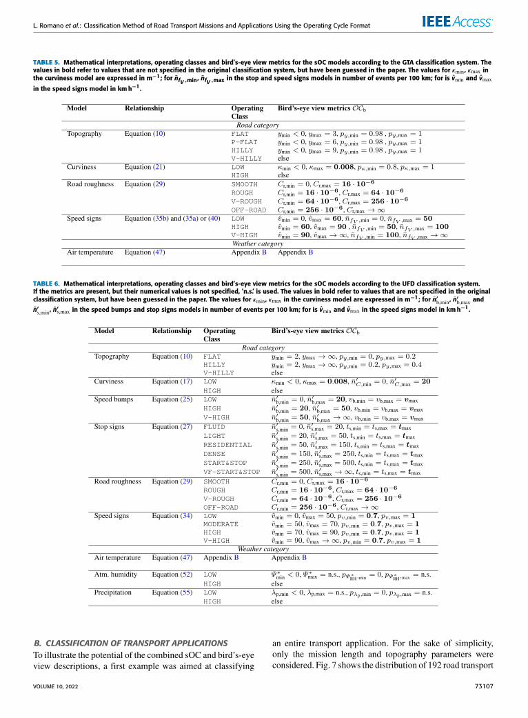
L. Romano et al.: Classification Method of Road Transport Missions and Applications Using the Operating Cycle Format
TABLE 5. Mathematical interpretations, operating classes and bird’s-eye view metrics for the sOC models according to the GTA classification system. Thevalues in bold refer to values that are not specified in the original classification system, but have been guessed in the paper. The values for κmin, κmax inthe curviness model are expressed in m−1; for n̄fV ,min, n̄fV ,max in the stop and speed signs models in number of events per 100 km; for is v̂min and v̂max
in the speed signs model in km h−1.
TABLE 6. Mathematical interpretations, operating classes and bird’s-eye view metrics for the sOC models according to the UFD classification system.If the metrics are present, but their numerical values is not specified, ’n.s.’ is used. The values in bold refer to values that are not specified in the originalclassification system, but have been guessed in the paper. The values for κmin, κmax in the curviness model are expressed in m−1; for n̄′b,min, n̄′b,max andn̄′s,min, n̄′s,max in the speed bumps and stop signs models in number of events per 100 km; for is v̂min and v̂max in the speed signs model in km h−1.
B. CLASSIFICATION OF TRANSPORT APPLICATIONSTo illustrate the potential of the combined sOC and bird’s-eyeview descriptions, a first example was aimed at classifying
an entire transport application. For the sake of simplicity,only the mission length and topography parameters wereconsidered. Fig. 7 shows the distribution of 192 road transport
VOLUME 10, 2022 73107

L. Romano et al.: Classification Method of Road Transport Missions and Applications Using the Operating Cycle Format
missions carried out by a Volvo FH16 during a period ofapproximately six months.8 The operations were classifiedusing the relationship for the OC class given by (10). Specifi-cally, Fig. 7(a) and Fig. 7(b) refer to the distributions obtainedaccording to the GTA and UFD thresholds for the standarddeviation σY of the road grade, as listed in Table 2. Whilethe total distance may be deduced immediately from log data,the topography parameters should be estimated using ad-hoctools, such as the Wafo package [94], [95].
Looking at Fig. 7, it may be observed that the two sys-tems yield rather different results. In particular, the UFDdescription misses the P-FLAT level; the transport opera-tions are, therefore, spread across the remaining categories.This generally increases the number of FLAT and HILLYmissions, compared to the distribution obtained by usingthe GTA metrics. Specifically, the HILLY category seemsto be predominant in Fig. 7(b), whereas the majority of themission is labeled as P-FLAT in Fig. 7(a). On the other hand,the distribution of V-HILLY missions is characterized by asimilar trend for both classification systems.
In both cases, the entire application may be character-ized starting with the estimated parameters for the individualmissions, combined with their distributions. Independentlyof the classification system, the application is labeled asL-DISTANCE in respect of the mission length, with anaverage distance traveled of 52.4 km. On the other hand, theGTA and UFD systems classify the application respectivelyas P-FLAT and HILLY in reference to the topography class.Additional details about the individual missions are given inTable 11 in Appendix C1.
C. CLASSIFICATION OF TRANSPORT MISSIONSConsidering individual road missions, an idealizedrepresentation in terms of a dOC may be built starting frommeasured data. An equivalent statistical description in theform of an sOCmay then be derived for each dOC by estimat-ing the stochastic parameters of the road models presentedin Section III.The following example analyzes six different sOCs,
parameterized using data collected during real vehicular oper-ations [58], [96]. To obtain a more accurate description of theoperating environment, the sOC parameters were estimatedfor different road types (urban, rural, highway). These weredetermined based on the legal speed values for differentsections (more details may be found in Appendix A). Thecomplete set of parameters for each reference sOC is listedin Tables 12, 13, 14, 15, 16 and 17 in Appendix C2. In gen-eral, it may be observed that each road type has its owncharacteristics. For instance, urban roads generally appearto be curvy, whereas rural and highway sections are mainlystraight, and characterized by longer and larger curves. Also,the frequency of stop signs may be expected to correlate tothe road type, as confirmed by the value of the parameters
8Since the example excludes the weather parameters, six months has beenassumed a sufficient period of time to span the overall application.
in Appendix C2. The classification of individual road typeswas then carried out directly by utilizing the expressions forthe operating classes derived in this paper. These, combinedwith (66) and (68) in Appendix C2, were finally used tocategorize each road mission (sOC).
The six operating cycles thus parametrized were then clas-sified, taking four different parameters into account: topogra-phy, curviness, stop and speed signs. Starting from the valuesfor the probabilities and metrics reported in Tables 5 and 6,the estimated classes for each combination of parameterand road type are listed in Table 7. Specifically, while boththe GTA and UFD systems set their own thresholds on themodel for topography, curviness, and speed signs, it shouldbe observed that the GTA lacks the operating classes forthe stop signs. Therefore, the corresponding road types andthe overall sOC were only labeled according to the metricsused in the UFD representation. For each operating cycle,the road types were first categorized individually, and thenused together to classify the overall mission according tothe methodology illustrated in Appendix A. The percentagesdescribing the road composition in the second column cor-respond to the stationary probabilities πRGR = 0 for thecontinuous-time Markov process describing the sequence ofroad types in Appendix. A. Generally speaking, it may beobserved highways are the predominant road compositionfor most of the operating cycles. As a result, the total prob-abilities and expectations calculated using (66) are largelydetermined by the stochastic parameters for the highways.These are often characterized by relatively higher velocities,smoother curves, reduced hilliness, and fewer stops. Thus,the stochastic operating cycles themselves inherit the samecharacteristics, and are labeled accordingly. This justifies toa large extent the fact that they quite often seem to fall inthe same categories as the corresponding highway roads.In particular, the two parameters that deserve special atten-tion are the topography and the speed signs. Concerningthe former, the road types and stochastic operating cyclesof the example are noticeably categorized in the P-FLATlevel according to the GTA system. However, this categoryis absent in the UFD representation, which systematicallyassigns the labels FLAT or HILLY. Again, this discrepancy isinteresting, and confirms that the two systems conflict most ofthe time. A similar phenomenon may be observed in respectof the speed signs (to ensure a fair comparison, only thecriterion on the mean speed in (35b) was included in theexample, while the number of transitions was disregarded).By construction, urban sections are always labeled in the LOWcategory according to both the GTA and UFD descriptions.According to the UFD metrics, rural and highway roadsare alternatively labeled as MODERATE and HIGH or HIGHand V-HIGH, respectively, whereas the UFD system oftenreplaces the MODERATE level with the HIGH class, exceptfor sOC 6. For the case under consideration, all the ruralsections were labeled as MODERATE using the UFD crite-rion, whereas the highways, excluded sOC 5, as HIGH. TheGTA system also classifies as V-HIGH the highway section
73108 VOLUME 10, 2022

L. Romano et al.: Classification Method of Road Transport Missions and Applications Using the Operating Cycle Format
FIGURE 7. Distribution of road transport mission according to the GTA (a) and UFD (b) classification systems.
of sOC 4. At any rate, the stochastic operating cycles alwaysinherited the HIGH label. Two striking exceptions are sOC 2and sOC 5, which did not satisfy any criterion based onthe classification established by the UFD system. Indeed,no speed range of those in Table 5 dominates for more than70% of the traveled distance. This unexpected result is symp-tomatic and highlights the need for a refined classificationsystem, plus more scientific definitions of both the notionof a class per se and its corresponding metrics. Conversely,the GTA system tends to assign the label V-HIGH to urbanor rural sections, which are characterized by more frequenttransitions between speeds. In this case, highway roads alsoexerted the majority of the influence in determining the levelof the entire operating cycles, which were always classifiedas LOW except for sOC 5.
D. A CASE-STUDY EXAMPLE OF APPLICATIONWhile a complete, rigorous optimization problem is beyondthe scope of this paper, a simple example is adduced toillustrate the practical application of the OC format for thepurpose of vehicle design selection. For the sake of sim-plicity, only two different configurations are considered andcompared in the following: a rigid Volvo FH16 750 and aFH13 540. The two configuration are similar, with the VolvoFH13 540 being equipped with a smaller engine. Additionaldetails about both configurations may be found, for example,in the Volvo specification sheets [97].
The energy performance of the two different powertrainsmay be assessed considering a typical transport applica-tion, given for example in the form of a distribution as inSection IV-B. To this end, multiple dOCs (either originalor synthetic) may be used as an input to a complete simu-lation model for longitudinal vehicle dynamics, including adynamic driver model. For the case study presented in thispaper, the VehProp environment [98] was used to model and
simulate both trucks. To reduce the dimension of the problem,a few sOCs were selected appropriately to be representativeof the actual usage. More specifically, using the GTA descrip-tion as a reference classification system, the first three sOCin Section IV-C, parametrised based on real data logged fromthe Volvo FH16 750, were employed to assess variability infuel consumption (measured in l 10−1km−1)9 depending onthe characteristics of each mission and on the specific config-uration. In this context, it may be easily observed that all thethree missions are classified as P-FLAT in the topographycategory, which is the predominant class. In turn, the selectedsOCs were used to synthesize 200 dOCs for each referencemission.
The resulting distributions are plotted in Figures 8 and 9.In particular, in Figure 8, the histograms of the fuel consump-tion are shown (blue for the FH16 750 and orange for theFH13 540), along with the mean value µ and the two band-widths µ±σ and µ±2σ (the corresponding mean values arelisted in Table 8 for both trucks), whereas Figure 9 comparesthe energy performance of the two configurations for eachreference mission. Generally speaking, it may be observedthat the total fuel consumption calculated by simulating thereference dOCs is lower than the mean value resulting fromthe corresponding distribution. For the first two missions,the fuel consumption in output from the reference dOCs isstill contained within a single standard deviation bandwidth,whereas for the third missions is contained between twostandard deviations for both vehicle configurations. There-fore, the reference dOCs may be fairly considered as typicaloperation for the first two transport missions. In all cases,it may be concluded that the FH13 540 outperforms the FH16750 in terms of energy efficiency, implying that, all the other
910 km correspond to one Swedish mil.
VOLUME 10, 2022 73109

L. Romano et al.: Classification Method of Road Transport Missions and Applications Using the Operating Cycle Format
TABLE 7. Operating classes for the six different stochastic operating cycles in the example of Section IV-C. The term composition refers to thecomposition of the road (percentages of urban, rural and highway types) according to the distributions calculated as explained in Section VI-A. Theclassification is carried out in respect of both the individual road types and the total transport operation. The topography and curviness parameters areclassified using the GTA and UFD system in turn; the stop signs are only classified using the metrics from the UFD.
TABLE 8. Fuel consumption (l10−1km−1).
things being equal, the FH13 540 configuration would bepreferable to purchase.10
It should be emphasized that, since only two different con-figurations were considered in the previous example, it waspossible to easily compare the energy performance on thewhole population of generated dOCs. This approach wouldnot be feasible when dealing with a complex optimizationproblem involving thousands of decision variables and pos-sible vehicle designs. In the latter case, the vehicle should
10In general, no substantial difference between the vehicles’s speed couldbe observed in simulation.
be optimized by considering dOCs that are optimally repre-sentative of both the mission characteristics and the energyusage, that is a synthetically generated mission yielding,in simulation, mean or close-to-mean energy consumption.Such approach as been already applied by other scholars,for example in [21]–[23], [26] (in particular, it is interestingto observe that the OC model for topography was alreadyincluded in [23], with the corresponding classes definedaccording to the GTA system). Moreover, if log data fromidividual or single vehicles are available, typical dOCs maybe properly selected as already explained in the previousexample. The representativeness in terms of energy consump-tion for an optimized configuration may be instead evaluateda posteriori on the same population of road operations.
V. DISCUSSIONThe examples in Section IV were aimed at illustrating howthe dual description bird’s-eye view/sOC can bemade toworkin practice when addressing the classification problem. Thissection discusses two extremely delicate aspects related to theproposed approach.
A. SCIENTIFIC DEFINITION OF METRICS AND LABELSThe example discussed in Section IV was emblematic inunderlining the need for a classification system that couldappropriately reflect the usage. To clarify this concept, one
73110 VOLUME 10, 2022

L. Romano et al.: Classification Method of Road Transport Missions and Applications Using the Operating Cycle Format
FIGURE 8. Distribution of the fuel consumption for both configurations.
FIGURE 9. Comparison between the distribution of the fuel consumption for each reference mission.
may think of a customer who, based on the known proper-ties of the intended transport application, needs to choosea new vehicle. Assuming that an optimization problem tofind standard configurations that better suit the applicationhas already been solved, the customer simply has to choosefrom the available optimal designs. However, the outcome ofthe optimization problem would be highly dependent on howthe operating classes and their metrics have been established.Both the GTA and UFD representations set their own systemsof thresholds mostly on empirical bases. The reason for thislies in the fact that both classifications have been developedover many years as a result of mutual interaction betweenmanufacturers and customers. Their non-mathematical nature
reflects the stakeholders’ necessities. In this context, the sub-stantial discrepancy between the metrics from the GTA andUFD systems might lead to very different solutions in termsof the best design. This might be overcome if a systematic,scientific method of specifying labels and limits for the oper-ating classes were to be established.
For those models whose metrics are prescribed in termsof expectation, as in (17), (25) and (27), the problem merelyreduces to finding the right sequence of limits for the expectednumber of events. This operation might seem trivial in theory,but, from a practical perspective, it is not obvious how toproceed. When the classes are specified in terms of probabil-ities, on the other hand, the issue may become rather thorny.
VOLUME 10, 2022 73111
L. Romano et al.: Classification Method of Road Transport Missions and Applications Using the Operating Cycle Format
Often, the GTA and UFD systems only set one bound. In thiscase, as with the road topography, the levels are always well-defined, and it is possible to assign a unique set of sOCparameters to a certain operating class. In a more generalsituation, lower and upper bounds on both the probabilityand the parameter itself should be prescribed to span theentire range of possibilities. However, this also multiplies thenumber of classes needed, increasing the complexity of sucha classification system. To keep the structure of a bird’s-eyeview description as simple as possible, it becomes obviousthat the thresholds values cannot be imposed based on puremathematical considerations, whereas a heuristic approach isrequired.
B. FEASIBLE SETS OF sOC PARAMETERSIt was briefly mentioned in Section II-D that the relation-ship between the bird’s-eye view and sOC representations isnot bijective in the ascending direction. In particular, whilea given set of sOC parameters should ideally corresponduniquely to a certain class, the opposite does not hold. Fix-ing a probability threshold, or equivalently the number ofexpected events, the analytical expression for an operatingclass may be interpreted as a hypersurface having multiplesolutions. Broadly speaking, there exist infinite different setsof sOC parameters that categorize a mission in the sameoperating class. Mathematically, this certainly appears log-ical. The physical interpretation, on the other hand, is notso obvious: some combinations of sOC parameters maymake no sense. An emblematic situation where this becomesproblematic is in dealing directly with customers, with noprior information about the intended usage: they may have arough idea of the characteristics of the operating environment,but would be unable to indicate a precise estimate of thetopography variance. The manufacturer might suggest anoptimal configuration for the truck based on the bird’s-eyeview description provided by the customer, but the optimiza-tion problem should have been already solved assuming aset of possible values for the topography variance. In thiscontext, how to ascertain that a solution is feasible fromthe physical interpretation perspective is a highly intriguingquestion. One possibility is to resort almost exclusively tosets of parameters extracted from real vehicular operations,or from data collected by external servers. Single missionsmight, therefore, be used as a basis to build a large, reliabledataset of parameters.
VI. CONCLUSIONClassifying individual transport missions at an individuallevel, as well as entire vehicular applications, is crucialwhen it comes to designing and selecting single componentsand configurations, and in the planning of maintenance andoptimization of road operations. This paper addressed theclassification problem from the perspective of the operatingcycle (OC) description by exploring the relationship betweentwo of its three levels of representation, namely the bird’s-eye view and the stochastic operating cycle (sOC). While
the former is characterized by a rather colloquial tone andaims to provide an intuitive understanding of the usageby resorting to simple metrics and labels, the latter is themost adequate descriptive tool in reflecting variation in theoperating environment, drivers’ attitudes, and overall vehicleperformance. Specifically, the non-technical language of thebird’s-eye view relies naturally on vague statements, whichmight be interpreted in terms of elementary statistics. On theother hand, the sOC represents the surroundings, includingthe road, weather, and traffic properties, using a vast setof independent stochastic models structured in a modular,hierarchical fashion.
In this paper, the natural connection between the sOCand the bird’s-eye view was therefore formulated in termsof elementary statistical operators, such as probability P(·)and expectation E(·). Starting from the stochastic modelingapproach typical of the sOC, these were calculated analyt-ically in Section III for the different models in the road,weather, and traffic categories, establishing algebraic expres-sions, renamed in this paper as operating classes, whichrelate the two levels of description. The result is a collectionof analytical relationships, which are easy to understand interms of frequencies, probabilities, and expected number ofevents that a driver may encounter along the road or duringa mission. In particular, the mathematical derivation of theexpressions for the operating classes was based on intuitiongained from examining some existing classification systems,like the Global Transport Application (GTA) introduced byVolvo and the User Factor Description (UFD) used by Scania.The purpose of the operating class is twofold. Exploitingthe relationship between the sOC and the bird’s-eye view inthe ascending direction, road transport missions categorizedaccording to the operating classes may be labeled directlystarting from, say, log data or non-technical informationretrieved from customers. This enables classification not onlyof road operations seen in isolation, but also the entire appli-cation, allowing for a high level of standardization. On theother hand, the non-bijective nature of the inverse relationship(in the descending direction) may facilitate optimization ofthe vehicle’s configuration, starting from a rough understand-ing of the usage. A typical case is that of a vehicle manu-facturer dealing with a customer, who cannot be expected tohave a deep knowledge of stochastic models and statisticaloperators. Asking simple questions about the typical operat-ing environment and characteristics of the mission, engineersmay use information from the answers to parametrize severalsOCs, and, in turn, dOCs. These may be combined with vehi-cle and driver models into virtual simulation environments toconduct statistical studies and solve optimization problems.
To illustrate the potential of the proposed approach,an example with six stochastic operating cycles parametrizedfrom log data, plus an entire transport application, was dis-cussed in Section IV, using the GTA and UFD systems forcomparison. While it was shown how to take advantage ofthe dual-level of description bird’s-eye view/sOC to catego-rize both individual roads and missions, the example also
73112 VOLUME 10, 2022

L. Romano et al.: Classification Method of Road Transport Missions and Applications Using the Operating Cycle Format
highlighted some weaknesses of the classification systemscurrently used. In particular, the need for more refined classi-fication criteria emerged in conjunctionwith the impossibilityof labeling certain missions, at least according to the metricsdefined in the GTA and UFD representations. How to pre-scribe probabilities and thresholds scientifically is howeveran open problem, which has not so far been explored incontext. Moreover, a unique operating class according to thebird’s-eye view description may correspond to sets of sOCparameters that are unfeasible from a physical perspective.Further research is needed to investigate both aspects ingreater detail.
Another interesting direction for future studies connectsto the possibility of including more stochastic models andparameters when addressing the classification problem ofenergy usage of road vehicles. For example, factors likeroad width, visibility, snow accumulation, wind speed anddirection, and daily traveled distance also play an importantrole in determining the vehicle’s response in terms of energyefficiency. However, they are not currently considered bythe existing classification systems. Therefore, the need forextending the stochastic operating cycle representation toincorporate these variables should be carefully evaluated.
Finally, the potential of the new formalism establishedin the paper should also be tested on large, compli-cated optimization problems, similar to those solved byGhandriz et al. [23], where the effect of the road topographywas investigated using the stochastic model discussed inSection III-A1. With the novel operating classes derived inSection III, the analysis conducted in [23] could be easilyextended to account for the contribution of other road andweather parameters.
APPENDIXA. ROAD TYPES AND TOTAL PROBABILITYThe notion of an operating class introduced in Sections II,and III may be used to categorize either a road mission or anindividual road section, hereinafter referred to as type. In thelatter case, the road type may be regarded as a primary modelfor the road, and would work similarly to the season for theweather category. Depending on the road type, different setsof stochastic parameters may then be used for the modelsillustrated in Section III, which would be treated as secondaryones. This approach is often used in the sOC representation,as discussed also in [58]. A graphical representation of thehierarchical structure of the road type, plus the sOC parame-ters for the secondary road models, is shown in Fig. 10. Morespecifically, the modeling of the road types may be relatedto the notion of speed signs, and represented as a stochasticprocess starting from the speed limit [99]. The existenceof nr different road types rt may be firstly postulated, i.e.{r1, . . . , rnr }, based on a sequence of nr − 1 characteristicspeeds, ordered in ascending magnitude. These would markthe transition from one road type to the next, implying thateach speed sign would belong uniquely to a given road type.
Accordingly, the road type would itself become a randomvariable Rt, assuming values rt ∈ SRt = {r1, . . . , rnr }, as afunction of the speed sign V (x), and would in turn dependon the position along the road. A specific number nv|ri ofspeed signs may be associated with each road type. Modelingthe locations Xk for the road types as in (14), the modelwould be described by a continuous-time Markov chain, andcompletely parametrized by the entries pRij of the single-steptransition matrix PR ∈ Rnr×nr
≥0 and the nr intensities λRi,reading
λRi =1LRi, (64)
being LRi the mean length of the road type ri. Again, thenr mean lengths LRi may be collected in a vector LR =[LR1 . . . LRnr ]
T.If a similar approach is preferred, analogous to that in
Section III-A5, the stationary πR distribution of the overallprocess should be derived as the solution of πRGR = 0,where the entries gRij = gRij(pRij,LRi) of the generator matrixGR would be given by
gRij(pRij,LRi
)=
λRipRij =
pRijLRi
, i 6= j,
−λRi = −1LRi, i = j.
(65)
To classify an operating cycle, it would therefore be necessaryto compute the total probabilities or expectations by sum-mation over the different road types. Indeed, road segmentsbelonging to the same road type should be described usingthe same values for the sOC parameters. The total probabilityand expectation for a generic random variable A in the roador weather categories would become
P(A) =nr∑i=1
P(A | Rt = ri)P(Rt = ri)
=
nr∑i=1
P(A | Rt = ri)πRi(PR,LR), (66a)
E(A) =nr∑i=1
E(A | Rt = ri)P(Rt = ri)
=
nr∑i=1
E(A | Rt = ri)πRi(PR,LR), (66b)
where the analytical expressions for the probabilitiesP(A | Rt = ri) and the expectations E(A | Rt = ri)would coincide with those for the operating classes derivedin Section III. It should be emphasized that, in (66), theprobabilities P(Rt = ri) may be set equal to the stationaryones for the road types, given a generic sOC. This shouldbe the preferred approach when referring to an sOC, whichis an abstract entity. In this context, it could be mentionedthat calculation of the number of transitions between speedsshould be modified to include also the number of transitionsbetween different road types. Introducing a new variable
VOLUME 10, 2022 73113

L. Romano et al.: Classification Method of Road Transport Missions and Applications Using the Operating Cycle Format
FIGURE 10. Graphical illustration of the primary road model.
TABLE 9. Upper and lower limits on the air temperature according to theGTA classification system.
NfV+fR = NfV+NfR , accounting for both types of speed jumps,the expected number of total transitions may be estimated as
E(NfV+fRLtot
)=
nr∑i=1
E(NfVLtot
∣∣∣∣ Rt = ri
)P(Rt = ri)
+ E(NfRLtot
)=
nr∑i=1
E(NfVLtot
∣∣∣∣ Rt = ri
)πRi(PR,LR)
+ E(NfRLtot
), (67)
where E(NfV /Ltot | Rt = ri) reads as in (39) and E(NfR/Ltot)may be calculatedwith similar relationships to (36), (37), (38)and (39).
Finally, the traffic density also deserves special attention,since its parameters would depend not only on road type butalso speed signs. Since each speed signmay be uniquely asso-ciated with a single road type, the total probability P(ρ∗min <
ρt ≤ ρ∗max) would be calculated as
P(ρ∗min < ρt ≤ ρ∗max)
=
nr∑i=1
nv|ri∑j=1
P(ρ∗min < ρt ≤ ρ∗max | Rt = ri ∩ V = vj)
× P(V = vj | Rt = ri)P(Rt = ri)
TABLE 10. The operating classes for the air temperature parameter in theUDF description. The V-COLD, COLD, WARM and V-WARM classes are definedby three relationships of the same type. On the other hand, the MIXEDclass only needs two inequalities to be completely defined.
=
nr∑i=1
nv|ri∑j=1
P(ρ∗min < ρt ≤ ρ∗max | Rt = ri ∩ V = vj)
×πVj(PV |ri ,LV |ri )πRi(PR,LR), (68)
where the formal expression for P(ρ∗min < ρt ≤ ρ∗max | Rt =
ri ∩ V = vj) would read exactly as in (63).
B. THE AIR TEMPERATURE PARAMETER IN THE GTA ANDUFD CLASSIFICATION SYSTEMSThe temperature parameter in the GTA and UFD classifi-cation systems is treated differently and deserves specialattention. In particular, the GTA description specifies thelower and upper bound on the thresholds T ∗min and T ∗max(Table 9). From Table 9, it may be understood there are eightpossible combinations between the upper and lower limits,
73114 VOLUME 10, 2022
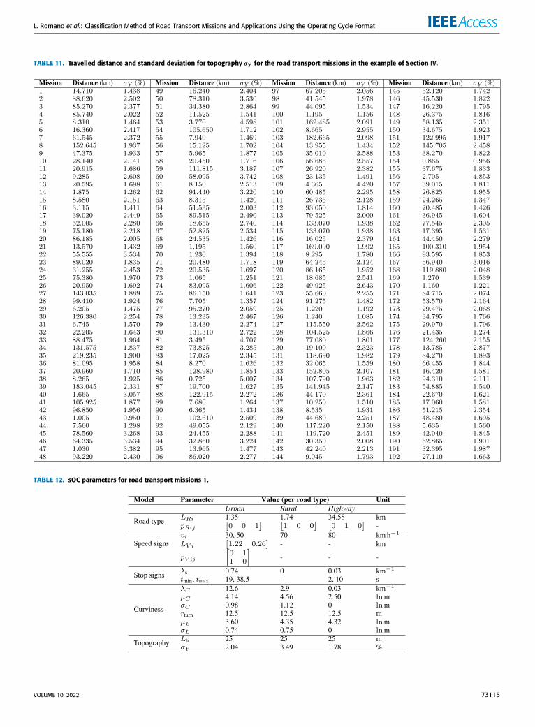
L. Romano et al.: Classification Method of Road Transport Missions and Applications Using the Operating Cycle Format
TABLE 11. Travelled distance and standard deviation for topography σY for the road transport missions in the example of Section IV.
TABLE 12. sOC parameters for road transport missions 1.
VOLUME 10, 2022 73115

L. Romano et al.: Classification Method of Road Transport Missions and Applications Using the Operating Cycle Format
TABLE 13. sOC parameters for road transport missions 2.
TABLE 14. sOC parameters for road transport missions 3.
TABLE 15. sOC parameters for road transport missions 4.
73116 VOLUME 10, 2022

L. Romano et al.: Classification Method of Road Transport Missions and Applications Using the Operating Cycle Format
TABLE 16. sOC parameters for road transport missions 5.
TABLE 17. sOC parameters for road transport missions 6.
and therefore eight possible classes.11 Accordingly, eachoperating class only needs one relationship to be completelydetermined.
On the other hand, the UFD description uses amore sophis-ticated strategy. Five levels are specified as follows:
1) V-COLD if sometimes colder than −30◦C, rarelywarmer than 20◦C and never warmer than 30◦C.
2) COLD if sometimes colder than −15◦C, rarely warmerthan 25◦C, and never warmer than 25◦C.
3) MIXED if rarely colder than −15◦C and rarely warmerthan 30◦C.
4) WARM if sometimes colder than 5◦C, never colderthan 0◦C and rarely warmer than 40◦C.
11In each case, the corresponding probability pT ∗air,max could be assumed
to be close to the unity (for example pT ∗air,max = 0.99) when it is not possibleto define a class using unit probabilities.
5) V-WARM if rarely colder than 15◦C, never colderthan 0◦C and sometimes warmer than 45◦C.
However, in the list above, the classes are formulated rathervaguely, since ’sometimes’ and ’rarely’ are not specified interms of frequencies or probabilities. As a first interpreta-tion, they may be assumed to indicate frequencies of aroundfifty and twenty percent, respectively (in bold in Table 10).Moreover, in the UFD system, each class is determined usingmultiple conditions on the limits T ∗min, T
∗max and the proba-
bility pT ∗air . These conditions may be numbered consecutivelyusing superscript (i), with i = 1, 2, 3 for the V-COLD, COLD,WARM and V-WARM classes, and i = 1, 2 for the MIXEDclass. Table 10 summarizes the operating classes for the airtemperature parameter according to the UFD interpretation.
However, in respect of the operating classes defined usingthe values in Tables 9 and 10, however, it should be observedthat the relationship (47) does not guarantee absolute lower
VOLUME 10, 2022 73117

L. Romano et al.: Classification Method of Road Transport Missions and Applications Using the Operating Cycle Format
and upper limits on the air temperature (apart from the zeropoint for thermodynamics). An alternative, and much simplerapproach, would consists in neglecting the stochastic com-ponent of the temperature, and only considering the annualvariation. In this case the probability P(Tair ≤ T ∗) becomes
P(Tair ≤ T ∗air) = FTair(T ∗air;µT ,Ty
)≈
12
+1πarctan
T ∗air − µT√T 2y − (µT − T ∗air)
2
, (69)
while the constraint on the lower and upper absolute limitsmay be expressed mathematically as
µT − Ty ≥ T ∗min, (70a)
µT + Ty ≤ T ∗max. (70b)
Equations (69) and (70) may be used in combination toprovide a feasible set of parameters satisfying the conditionsfor the operating classes. In particular, it is worth mentioningthat the different levels specified by the GTA system onlyneed (70).
C. ADDITIONAL DATA AND TABLES1) DATA FOR INDIVIDUAL MISSIONSThe values for the traveled distance and the standard deviationσY of the topography for the missions in the example ofSection IV are listed in Table 11.
2) sOC PARAMETERSThe estimated parameters for the sOCs in the example ofSection IV-C are listed below. See Tables 12–17.
ACKNOWLEDGMENTThe authors kindly acknowledge the support from theCOVER Project Member Anders Jensen at Scania, whosupplied information on the User Factor Description (UFD).Authors Contribution: Luigi Romano—conceptualization,formalization, theory, methodology, formal analysis, imple-mentation, data analysis, and writing—original draft;Pär Johannesson—methodology and supervision; ErikNordström—implementation and data analysis; FredrikBruzelius—conceptualization and supervision; RickardAnderson—funding acquisition; and Bengt Jacobson—supervision and funding acquisition. All the authors read andapproved the original version of the manuscript.
REFERENCES[1] P. Pettersson, ‘‘Operating cycle representation for road vehicles,’’ Ph.D.
dissertation, Dept. Mech. Maritime Sci., Chalmers Univ. Technol.,Gothenburg, Sweden, 2019.
[2] S. Edlund and P.-O. Fryk, ‘‘The right truck for the job with globaltruck application descriptions,’’ in Proc. SAE Tech. Paper Ser., Oct. 2004,pp. 344–351, doi: 10.4271/2004-01-2645.
[3] G. Fontaras, M. Rexeis, P. Dilara, S. Hausberger, and K. Anagnostopoulos,‘‘Development of a simulation tool for monitoring heavy-duty vehicleCO2 emissions and fuel consumption in Europe,’’ in Proc. 11th Int. Conf.Engines Vehicles, 2013, pp. 1–11.
[4] H. Achour andA. G. Olabi, ‘‘Driving cycle developments and their impactson energy consumption of transportation,’’ J. Cleaner Prod., vol. 112,pp. 1778–1788, Jan. 2016, doi: 10.1016/j.jclepro.2015.08.007.
[5] J. Liu, X. Wang, and A. Khattak, ‘‘Customizing driving cycles to sup-port vehicle purchase and use decisions: Fuel economy estimation foralternative fuel vehicle users,’’ Transp. Res. C, Emerg. Technol., vol. 67,pp. 280–298, Jun. 2016, doi: 10.1016/j.trc.2016.02.016.
[6] D. W. Wyatt, H. Li, and J. E. Tate, ‘‘The impact of road grade on carbondioxide (CO2) emission of a passenger vehicle in real-world driving,’’Transp. Res. D, Transp. Environ., vol. 32, pp. 160–170, Oct. 2014, doi:10.1016/j.trd.2014.07.015.
[7] K. M. Sentoff, L. Aultman-Hall, and B. A. Holmén, ‘‘Implications ofdriving style and road grade for accurate vehicle activity data and emis-sions estimates,’’ Transp. Res. D, Transp. Environ., vol. 35, pp. 175–188,Mar. 2015, doi: 10.1016/j.trd.2014.11.021.
[8] D. Llopis-Castelló, A. M. Pérez-Zuriaga, F. J. Camacho-Torregrosa, andA. García, ‘‘Impact of horizontal geometric design of two-lane rural roadson vehicle co 2 emissions,’’ Transp. Res. D, Transp. Environ., vol. 59,pp. 46–57, Mar. 2018, doi: 10.1016/j.trd.2017.12.020.
[9] A. Sciarretta, Energy-Efficient Driving of Road Vehicles, 1st ed. Cham,Switzerland: Springer, 2020, doi: 10.1007/978-3-030-24127-8.
[10] P. Johannesson, K. Podgórski, I. Rychlik, and N. Shariati, ‘‘AR(1) timeseries with autoregressive gamma variance for road topography mod-eling,’’ Probabilistic Eng. Mech., vol. 43, pp. 106–116, Jan. 2016, doi:10.1016/j.probengmech.2015.12.006.
[11] P. Johannesson, K. Podgórski, and I. Rychlik, ‘‘Laplace distributionmodels for road topography and roughness,’’ Int. J. Vehicle Perform.,vol. 3, no. 3, p. 224, 2017. [Online]. Available: http://www.inderscience.com/offer.php?id=85032
[12] A. Donkers, D. Yang, and M. Viktorović, ‘‘Influence of driving style,infrastructure, weather and traffic on electric vehicle performance,’’Transp. Res. D, Transp. Environ., vol. 88, Nov. 2020, Art. no. 102569, doi:10.1016/J.TRD.2020.102569.
[13] D. Akin, V. P. Sisiopiku, and A. Skabardonis, ‘‘Impacts of weather on traf-fic flow characteristics of urban freeways in Istanbul,’’ Proc. Social Behav.Sci., vol. 16, pp. 88–89, Jan. 2011, doi: 10.1016/J.SBSPRO.2011.04.432.
[14] E. Hooper, L. Chapman, and A. Quinn, ‘‘The impact of precipitation onspeed–flow relationships along a U.K. motorway corridor,’’ Theor. Appl.Climatol., vol. 117, nos. 1–2, pp. 303–316, Jul. 2014, doi: 10.1007/s00704-013-0999-5.
[15] O. Travesset-Baro, M. Rosas-Casals, and E. Jover, ‘‘Transport energyconsumption in mountainous roads. A comparative case study forinternal combustion engines and electric vehicles in andorra,’’ Transp.Res. D, Transp. Environ., vol. 34, pp. 16–26, Jan. 2015, doi: 10.1016/J.TRD.2014.09.006.
[16] B. Y. Boroujeni and H. C. Frey, ‘‘Road grade quantification based onglobal positioning system data obtained from real-world vehicle fuel useand emissions measurements,’’ Atmos. Environ., vol. 85, pp. 179–186,Mar. 2014, doi: 10.1016/j.atmosenv.2013.12.025.
[17] P. Shen, Z. Zhao, J. Li, and X. Zhan, ‘‘Development of a typicaldriving cycle for an intra-city hybrid electric bus with a fixed route,’’Transp. Res. D, Transp. Environ., vol. 59, pp. 346–360, Mar. 2018, doi:10.1016/j.trd.2018.01.032.
[18] J. Brady and M. O’Mahony, ‘‘Development of a driving cycle to evaluatethe energy economy of electric vehicles in urban areas,’’ Appl. Energy,vol. 177, pp. 165–178, Sep. 2016, doi: 10.1016/j.apenergy.2016.05.094.
[19] L. Guzzella and A. Sciarretta, Vehicle Propulsion Systems: Introduction toModeling and Optimization, 3st ed. Cham, Switzerland: Springer, 2013.
[20] T. Hofman, S. Ebbesen, and L. Guzzella, ‘‘Topology optimizationfor hybrid electric vehicles with automated transmissions,’’ IEEETrans. Veh. Technol., vol. 61, no. 6, pp. 2442–2451, Jul. 2012, doi:10.1109/TVT.2012.2196299.
[21] T. Ghandriz, J. Hellgren, M. Islam, L. Laine, and B. Jacobson, ‘‘Optimiza-tion based design of heterogeneous truck fleet and electric propulsion,’’in Proc. IEEE 19th Int. Conf. Intell. Transp. Syst. (ITSC), Nov. 2016,pp. 328–335.
[22] T. Ghandriz, ‘‘Transportation mission based optimization of heavy vehi-cle fleets including propulsion tailoring,’’ Licentiate thesis, Dept. Mech.Maritime Sci., Chalmers Univ. Technol., Gothenburg, Sweden, 2018.
[23] T. Ghandriz, B. Jacobson, L. Laine, and J. Hellgren, ‘‘Impact of automateddriving systems on road freight transport and electrified propulsion ofheavy vehicles,’’ Transp. Res. C, Emerg. Technol., vol. 115, Jun. 2020,Art. no. 102610, doi: 10.1016/j.trc.2020.102610.
73118 VOLUME 10, 2022

L. Romano et al.: Classification Method of Road Transport Missions and Applications Using the Operating Cycle Format
[24] T. Ghandriz, B. Jacobson, L. Laine, and J. Hellgren, ‘‘Optimization data ontotal cost of ownership for conventional and battery electric heavy vehiclesdriven by humans and by automated driving systems,’’ Data Brief, vol. 30,Jun. 2020, Art. no. 105566, doi: 10.1016/j.dib.2020.105566.
[25] T. Ghandriz, B. Jacobson, M. Islam, J. Hellgren, and L. Laine,‘‘Transportation-mission-based optimization of heterogeneous heavy-vehicle fleet including electrified propulsion,’’ Energies, vol. 14, no. 11,p. 3221, May 2021, doi: 10.3390/en14113221.
[26] T. Ghandriz, ‘‘Transportation mission-based optimization of heavy com-bination road vehicles and distributed propulsion, including predictiveenergy and motion contro,’’ Ph.D. dissertation, Dept. Mech. Maritime Sci.,Chalmers Univ. Technol., Gothenburg, Sweden, 2020.
[27] M. Åsbogård, L. Johannesson, D. Angervall, and P. Johansson, ‘‘Improv-ing system design of a hybrid powertrain using stochastic drivecycles and dynamic programming,’’ in Proc. SAE Tech. Paper Ser.,Apr. 2007, p. 10, doi: 10.4271/2007-01-0304.
[28] P. Nyberg, ‘‘Evaluation, generation and transformation of driving cycles,’’Ph.D. dissertation, Dept. Elect. Eng., Linköping Univ. Electronic Press,Linköping, Sweden, 2015.
[29] A. Ashtari, E. Bibeau, and S. Shahidinejad, ‘‘Using large driving recordsamples and a stochastic approach for real-world driving cycle construc-tion: Winnipeg driving cycle,’’ Transp. Sci., vol. 48, no. 2, pp. 170–183,May 2014, doi: 10.1287/trsc.1120.0447.
[30] E. Tazelaar, J. Bruinsma, B. Veenhuizen, and P. Bosch, ‘‘Driving cyclecharacterization and generation, for design and control of fuel cellbuses,’’ World Electr. Veh. J., vol. 3, no. 1, pp. 812–819, 2009, doi:10.3390/wevj3040812.
[31] J. Lin andD. A. Niemeier, ‘‘An exploratory analysis comparing a stochasticdriving cycle to California’s regulatory cycle,’’ Atmos. Environ., vol. 36,no. 38, pp. 5759–5770, 2002, doi: 10.1016/S1352-2310(02)00695-7.
[32] T.-K. Lee and Z. S. Filipi, ‘‘Synthesis of real-world driving cyclesusing stochastic process and statistical methodology,’’ Int. J.Vehicle Des., vol. 57, no. 1, pp. 17–36, 2011. [Online]. Available:http://www.inderscience.com/offer.php?id=43590
[33] T.-K. Lee, B. Adornato, and Z. S. Filipi, ‘‘Synthesis of real-worlddriving cycles and their use for estimating PHEV energy consump-tion and charging opportunities: Case study for midwest/U.S.,’’ IEEETrans. Veh. Technol., vol. 60, no. 9, pp. 4153–4163, Nov. 2011, doi:10.1109/TVT.2011.2168251.
[34] G. Amirjamshidi and M. J. Roorda, ‘‘Development of simulated drivingcycles for light, medium, and heavy duty trucks: Case of the Toronto water-front area,’’ Transp. Res. D, Transp. Environ., vol. 34, no. 1, pp. 255–266,2015, doi: 10.1016/j.trd.2014.11.010.
[35] S. H. Kamble, T. V. Mathew, and G. K. Sharma, ‘‘Development of real-world driving cycle: Case study of Pune, India,’’ Transp. Res. D, Transp.Environ., vol. 14, no. 2, pp. 132–140, 2009, doi: 10.1016/j.trd.2008.11.008.
[36] E. Silvas, ‘‘Integrated optimal design for hybrid electric vehicles,’’Ph.D. dissertation, Dept. Mech. Eng., Technische Universiteit Eindhoven,Eindhoven, The Netherlands, 2015.
[37] E. Silvas, K. Hereijgers, H. Peng, T. Hofman, and M. Steinbuch, ‘‘Synthe-sis of realistic driving cycles with high accuracy and computational speed,including slope information,’’ IEEE Trans. Veh. Technol., vol. 65, no. 6,pp. 4118–4128, Mar. 2016, doi: 10.1109/TVT.2016.2546338.
[38] X. Liu, J. Ma, X. Zhao, J. Du, and Y. Xiong, ‘‘Study on drivingcycle synthesis method for city buses considering random passengerload,’’ J. Adv. Transp., vol. 2020, pp. 1–21, Feb. 2020, doi: 10.1155/2020/3871703.
[39] S. Shi, S. Wei, H. Kui, L. Liu, C. Huang, and M. Liu, ‘‘Improvementsof the design method of transient driving cycle for passenger car,’’ inProc. IEEE Vehicle Power Propuls. Conf., Sep. 2009, pp. 1581–1586, doi:10.1109/VPPC.2009.5289594.
[40] L. Liu, C. Huang, M. Liu, and S. Shi, ‘‘Study on the combined designmethod of transient driving cycles for passenger car in Changchun,’’ inProc. IEEE Vehicle Power Propuls. Conf., Sep. 2008. [Online]. Available:https://ieeexplore.ieee.org/stamp/stamp.jsp?arnumber=4677594
[41] W. T. Hung, H. Y. Tong, C. P. Lee, K. Ha, and L. Y. Pao, ‘‘Development ofa practical driving cycle construction methodology: A case study in HongKong,’’ Transp. Res. D, Transp. Environ., vol. 12, no. 2, pp. 115–128, 2007,doi: 10.1016/j.trd.2007.01.002.
[42] K. S. Nesamani and K. P. Subramanian, ‘‘Development of a driving cyclefor intra-city buses in Chennai, India,’’ Atmos. Environ., vol. 45, no. 31,pp. 5469–5476, 2011, doi: 10.1016/j.atmosenv.2011.06.067.
[43] S.-H. Ho, Y.-D. Wong, and V. W.-C. Chang, ‘‘Developing Singaporedriving cycle for passenger cars to estimate fuel consumption and vehic-ular emissions,’’ Atmos. Environ., vol. 97, pp. 353–362, Nov. 2014, doi:10.1016/j.atmosenv.2014.08.042.
[44] K. Kivekäs, J. Vepsäläinen, and K. Tammi, ‘‘Stochastic drivingcycle synthesis for analyzing the energy consumption of a bat-tery electric bus,’’ IEEE Access, vol. 6, pp. 55586–55598, 2018, doi:10.1109/ACCESS.2018.2871574.
[45] K. Kivekas, J. Vepsalainen, K. Tammi, and J. Anttila, ‘‘Influence ofdriving cycle uncertainty on electric city bus energy consumption,’’ inProc. IEEE Vehicle Power Propuls. Conf. (VPPC), Dec. 2017, pp. 1–5, doi:10.1109/VPPC.2017.8331014.
[46] F. Guo and F. Zhang, ‘‘A study of driving cycle for electric cars on Beijingurban and suburban roads,’’ in Proc. IEEE Int. Conf. Power Renew. Energy(ICPRE), Oct. 2016, pp. 319–322, doi: 10.1109/ICPRE.2016.7871224.
[47] S. Ou, Y. Zhou, J. Lian, P. Jia, and B. Tian, ‘‘Development of hybrid citybus’s driving cycle,’’ inProc. Int. Conf. Electr. Inf. Control Eng., Apr. 2011,pp. 2112–2116, doi: 10.1109/ICEICE.2011.5777149.
[48] L. Berzi, M. Delogu, and M. Pierini, ‘‘Development of driving cyclesfor electric vehicles in the context of the city of Florence,’’ Transp.Res. D, Transp. Environ., vol. 47, pp. 299–322, Aug. 2016, doi: 10.1016/j.trd.2016.05.010.
[49] S. Shi, N. Lin, Y. Zhang, C. Huang, L. Liu, B. Lu, and J. Cheng,‘‘Research on Markov property analysis of driving cycle,’’ in Proc.IEEE Vehicle Power Propuls. Conf. (VPPC), Oct. 2013, pp. 1–5, doi:10.1109/VPPC.2013.6671737.
[50] X. Hu, N. Murgovski, L. M. Johannesson, and B. Egardt, ‘‘Optimaldimensioning and power management of a fuel cell/battery hybrid bus viaconvex programming,’’ IEEE/ASME Trans. Mechatronics, vol. 20, no. 1,pp. 457–468, Feb. 2015, doi: 10.1109/TMECH.2014.2336264.
[51] E. Silvas, T. Hofman, N. Murgovski, L. F. P. Etman, and M. Steinbuch,‘‘Review of optimization strategies for system-level design in hybridelectric vehicles,’’ IEEE Trans. Veh. Technol., vol. 66, no. 1, pp. 57–70,Jan. 2017, doi: 10.1109/TVT.2016.2547897.
[52] X. Hu, S. J. Moura, N. Murgovski, B. Egardt, and D. Cao, ‘‘Integratedoptimization of battery sizing, charging, and power management in plug-in hybrid electric vehicles,’’ IEEE Trans. Control Syst. Technol., vol. 24,no. 3, pp. 1036–1043, May 2016, doi: 10.1109/TCST.2015.2476799.
[53] M. Pourabdollah, N. Murgovski, A. Grauers, and B. Egardt, ‘‘Optimalsizing of a parallel PHEV powertrain,’’ IEEE Trans. Veh. Technol., vol. 62,no. 6, pp. 2469–2480, Jul. 2013, doi: 10.1109/TVT.2013.2240326.
[54] Z. Zou, S. Davis, K. Beaty, M. O’Keefe, T. Hendricks, R. Rehn,S. Weissner, and V. K. Sharma, ‘‘A new composite drive cycle for heavy-duty hybrid electric class 4–6 vehicles,’’ in Proc. SAE Tech. Paper Ser.,Mar. 2004, pp. 1–10, doi: 10.4271/2004-01-1052.
[55] M. Montazeri-Gh andM. Naghizadeh ‘‘Development of car drive cycle forsimulation of emissions and fuel economy,’’ in Proc. 15th Eur. SimulationSymp. Alexander Verbraesk, V. Hlupic, Ed. SCS European Council/SCSEurope BVBA, 2003.
[56] Z. Jing, G. Wang, S. Zhang, and C. Qiu, ‘‘Building Tianjin driving cyclebased on linear discriminant analysis,’’ Transp. Res. D, Transp. Environ.,vol. 53, pp. 78–87, Jun. 2017, doi: 10.1016/j.trd.2017.04.005.
[57] J. Vepsäläinen, K. Kivekäs, K. Otto, A. Lajunen, and K. Tammi, ‘‘Develop-ment and validation of energy demand uncertainty model for electric citybuses,’’ Transp. Res. D, Transp. Environ., vol. 63, pp. 347–361, Aug. 2018,doi: 10.1016/j.trd.2018.06.004.
[58] P. Pettersson, P. Johannesson, B. Jacobson, F. Bruzelius, L. Fast, andS. Berglund, ‘‘A statistical operating cycle description for prediction ofroad vehicles’ energy consumption,’’ Transp. Res. D, Transp. Environ.,vol. 73, pp. 205–229, Aug. 2019, doi: 10.1016/j.trd.2019.07.006.
[59] L. Romano, P. Johannesson, F. Bruzelius, and B. Jacobson, ‘‘An enhancedstochastic operating cycle description including weather and traffic mod-els,’’ Transp. Res. D, Transp. Environ., vol. 97, Aug. 2021, Art. no. 102878,doi: 10.1016/j.trd.2021.102878.
[60] P. Pettersson, S. Berglund, B. Jacobson, L. Fast, P. Johannesson, andF. Santandrea, ‘‘A proposal for an operating cycle description format forroad transport missions,’’ Eur. Transp. Res. Rev., vol. 10, no. 2, pp. 1–19,Jun. 2018, doi: 10.1186/s12544-018-0298-4.
[61] L. Romano, ‘‘Mathematical modelling of operating cycles for road vehi-cles,’’ Licentiate thesis, Dept. Mech. Maritime Sci., Chalmers Univ. Tech-nol., Gothenburg, Sweden, 2021.
[62] M. Karlsson, ‘‘Load modelling for fatigue assessment of vehicles—Astatistical approach,’’ Ph.D. dissertation, Dept. Math. Sci., Chalmers Univ.Technol., Göteborg, Sweden, 2007.
VOLUME 10, 2022 73119

L. Romano et al.: Classification Method of Road Transport Missions and Applications Using the Operating Cycle Format
[63] M. Karlsson, ‘‘Evaluation of approximative methods for rainflow damageof broad-banded non-Gaussian random loads,’’ in Proc. Design Eng., A B,Jan. 2005, pp. 79–87, doi: 10.1115/IMECE2005-79868.
[64] M. Karlsson, ‘‘Evaluation of road load classification for fatigue assess-ments,’’ Int. J. Vehicle Des., vol. 47, nos. 1–4, pp. 250–268, 2013, doi:10.1504/IJVD.2008.020890.
[65] K. Bogsjö, ‘‘Coherence of road roughness in left and right wheel-path,’’Vehicle Syst. Dyn., vol. 46, no. sup1, pp. 599–609, Sep. 2008, doi:10.1080/00423110802018289.
[66] P. Johannesson, K. Podgórski, and I. Rychlik, ‘‘Modelling roughness ofroad profiles on parallel tracks using roughness indicators,’’ Int. J. VehicleDes., vol. 70, no. 2, p. 183, 2016.
[67] K. Bogsjö, K. Podgórski, and I. Rychlik, ‘‘Models for road surfaceroughness,’’ Vehicle Syst. Dyn., vol. 50, no. 5, pp. 725–747, 2012, doi:10.1080/00423114.2011.637566.
[68] G. Box, G. Jenkins, G. Reinsel, G. Ljung, and G. Ljung, Time SeriesAnalysis: Forecasting and Control, 5th ed. San Francisco, CA, USA:Wiley, 2015.
[69] C. J. J. Beckers, I. J. M. Besselink, and H. Nijmeijer, ‘‘Modelingof energy losses during cornering for electric city buses,’’ in Proc.IEEE Intell. Transp. Syst. Conf. (ITSC), Oct. 2019, pp. 4164–4169, doi:10.1109/ITSC.2019.8917232.
[70] C. Beckers, I. Besselink, and H. Nijmeijer, ‘‘On-line test of a real-timevelocity prediction for E-bus energy consumption estimation,’’ in Proc.IEEE Vehicle Power Propuls. Conf. (VPPC), Oct. 2021, pp. 1–5, doi:10.1109/VPPC53923.2021.9699205.
[71] C. J. J. Beckers, I. J. M. Besselink, and H. Nijmeijer, ‘‘Assessing the impactof cornering losses on the energy consumption of electric city buses,’’Transp. Res. D, Transp. Environ., vol. 86, Sep. 2020, Art. no. 102360, doi:10.1016/j.trd.2020.102360.
[72] C. J. Dodds and J. D. Robson, ‘‘The description of road surface rough-ness,’’ J. Sound Vibrat., vol. 31, no. 2, p. 2, 1973, doi: 10.1016/S0022-460X(73)80373-6.
[73] Mechanical Vibration—Road Surface Profiles—Reporting of MeasuredData, document ISO 8608, 1995.
[74] F. Pellicano, Z. Li, W. Yu, and X. Cui, ‘‘Online classification of roadroughness conditions with vehicle unsprung mass acceleration by slid-ing time window,’’ Shock Vib., vol. 10, no. 3, pp. 1–14, 2018, doi:10.1109/TVT.2012.2196299.
[75] S. Kotz, T. Kozubowski, and K. Podgorski, The Laplace Distributionand Generalizations, 2nd ed. Basel, Switzerland: Birkhäuser, 2001, doi:10.1007/978-1-4612-0173-1.
[76] M. Guiggiani, The Science of Vehicle Dynamics, 2nd ed. Cham, Switzer-land: Springer, 2018.
[77] H. B. Pacejka, Tire and Vehicle Dynamics, 3rd ed. Amsterdam, The Nether-lands: Elsevier, 2012.
[78] L. Romano, F. Timpone, F. Bruzelius, and B. Jacobson, ‘‘Analytical resultsin transient brush tyre models: Theory for large camber angles and classicsolutions with limited friction,’’ Meccanica, vol. 57, no. 1, pp. 165–191,Jan. 2022, doi: 10.1007/s11012-021-01422-3.
[79] L. Romano, Advanced Brush Tyre Modelling. Cham, Switzerland:Springer, 2022, doi: 10.1007/978-3-030-98435-9.
[80] G. Grimmett and D. Stirzaker, Probability and Random Processes, 4th ed.London, U.K.: Oxford Univ. Press, 2020.
[81] H. P. Hsu, Schaum’s Outline of Probability, Random Variables, and Ran-dom Processes, 4th ed. New York, NY, USA: McGraw-Hill, 2020.
[82] R. Griego and R. Hersh, ‘‘Theory of random evolutions with applica-tions to partial differential equations,’’ Trans. Amer. Math. Soc., vol. 156,pp. 405–418, Jan. 1971, doi: 10.2307/1995620.
[83] K. L. Chungr, Markov Chains With Stationary Transition Probabilities,2nd ed. Berlin, Germany: Springer, 1967, doi: 10.1007/978-3-642-62015-7.
[84] A. R. Babu, J. Andric, B. Minovski, and S. Sebben, ‘‘System-level mod-eling and thermal simulations of large battery packs for electric trucks,’’Energies, vol. 14, no. 16, p. 4796, Aug. 2021, doi: 10.3390/en14164796.
[85] G. J. Marshall, C. P. Mahony, M. J. Rhodes, S. R. Daniewicz, N. Tsolas,and S. M. Thompson, ‘‘Thermal management of vehicle cabins, externalsurfaces, and onboard electronics: An overview,’’ Engineering, vol. 5,no. 5, pp. 954–969, Oct. 2019, doi: 10.1016/j.eng.2019.02.009.
[86] M. M. Ahmed and A. Ghasemzadeh, ‘‘The impacts of heavy rain on speedand headway behaviors: An investigation using the SHRP2 naturalisticdriving study data,’’ Transp. Res. C, Emerg. Technol., vol. 91, pp. 371–384,Jun. 2018, doi: 10.1016/j.trc.2018.04.012.
[87] J. Yeo, J. Lee, and K. Jang, ‘‘The effects of rainfall on driving behaviorsbased on driving volatility,’’ Int. J. Sustain. Transp., vol. 15, pp. 435–443,Mar. 2021, doi: 10.1080/15568318.2020.1756543.
[88] B. N. J. Persson, U. Tartaglino, O. Albohr, and E. Tosatti, ‘‘Rubber frictionon wet and dry road surfaces: The sealing effect,’’ Phys. Rev. B, Condens.Matter, vol. 71, no. 3, Jan. 2005, Art. no. 035428, doi: 10.1103/Phys-RevB.71.035428.
[89] K. R. Gabriel and J. Neumann, ‘‘A Markov chain model for daily rainfalloccurrence at tel aviv,’’ Quart. J. Roy. Meteorolog. Soc., vol. 88, no. 375,pp. 90–95, Jan. 1962, doi: 10.1002/qj.49708837511.
[90] E. H. Chin, ‘‘Modeling daily precipitation occurrence process withMarkovchain,’’ Water Resour. Res., vol. 13, no. 6, pp. 949–956, Dec. 1977, doi:10.1029/WR013i006p00949.
[91] G. J. Husak, J. Michaelsen, and C. Funk, ‘‘Use of the gamma distributionto represent monthly rainfall in Africa for drought monitoring applica-tions,’’ Int. J. Climatol., vol. 27, no. 7, pp. 935–944, Jun. 2007, doi:10.1002/joc.1441.
[92] V. Kumar and S. Jahangeer, ‘‘Statistical distribution of rainfall in Uttarak-hand, India,’’ Appl. Water Sci., vol. 7, no. 8, pp. 4765–4776, Dec. 2017,doi: 10.1007/s13201-017-0586-5.
[93] MANOBS (Manual of Surface Weather Observations), Metereological Ser-vice of Canada, Toronto, ON, Canada, 2013.
[94] P. A. Brodtkorb, P. Johannesson, G. Lindgren, I. Rychlik, J. Rydén, andE. Sjö, ‘‘WAFO—-AMATLAB Toolbox for the analysis of random wavesand loads,’’ Proc. 10th Int. Offshore Polar Eng. Conf., (ISOPE), vol. 3,2000, pp. 343–350.
[95] WAFO—A MATLAB Toolbox for Analysis of Random Waves and Loads—A Tutorial, WAFO-Group, Mathematics & Statistics, Centre for Mathe-matical Sciences, Lund Univ., Lund, Sweden, 2000. [Online]. Available:http://www.maths.lth.se/matstat/wafo
[96] E. Nordström, ‘‘Advanced modelling and energy efficiency prediction forroad vehicles,’’ M.S. thesis, Dept. Phys., Umeå Univ., Umeå, Sweden,2020.
[97] Volvotrucks.se. Accessed: Jul. 7, 2022. [Online]. Available: https://www.volvotrucks.se/sv-se/trucks/trucks/volvo-fh16/specifications/data-sheets.html
[98] VehProp. Accessed: Jul. 7, 2022. [Online]. Available: https://www.chalmers.se/en/departments/m2/research/veas/Pages/VehProp.aspx
[99] L. Ntziachristos and Z. Samaras,EMEP/EEAAir Pollutant Emission Inven-tory Guidebook 2016 Part B.1.A.3.B.I-Iv Road Transport 2018. Copen-hagen, Denmark: European Environment Agency, Chalmers Univ. Tech-nology, 2018.
LUIGI ROMANO received the M.Sc. degree inmechanical engineering from the University ofNaples Federico II, Italy, in 2018. He is cur-rently pursuing the Ph.D. degree with the VehicleDynamics Group, Chalmers University of Tech-nology, Gothenburg, Sweden, within the COVERProject. After graduation, he worked as an Inde-pendent Consultant on the Feel-Tire Unina Project,developing model-based estimators for intelligenttire technologies. His research interests include
sustainable transportation systems, vehicle state estimation and control, andtire dynamics and modeling. In 2016, he was awarded the prize ‘‘BuonCompleanno Federico II’’ as the Best Mechanical Engineering Student.
PÄR JOHANNESSON received the Ph.D.degree in mathematical statistics from the LundInstitute of Technology, with a thesis on statisti-cal load analysis for fatigue, and the joint post-doctoral degree in mathematical statistics fromthe Chalmers University of Technology and PSAPeugeot Citroën, France. He currently works asa Senior Researcher in mechanical reliability,fatigue, and load analysis at RISE Research Insti-tute of Sweden, Gothenburg. He is a Docent in
mathematical statistics with the Chalmers University of Technology. He hasmore than 20 years of experience in research and development in fatigueand loads analysis with a focus on engineering statistics and reliability inindustrial applications. He has published more than 20 articles in interna-tional journals and is a Co-Editor of the handbook Guide to Load Analysisfor Durability in Vehicle Engineering.
73120 VOLUME 10, 2022

L. Romano et al.: Classification Method of Road Transport Missions and Applications Using the Operating Cycle Format
ERIK NORDSTRÖM received the degree in engi-neering physics from Umeå University, Sweden,in 2020. He carried out his master’s thesiswork at the Chalmers University of Technology,Gothenburg, Sweden, where he was also involvedin the COVER Project. He is currently a PostGraduate Student at Umeaå University and a QATest Engineering at Nasdaq, Stockholm.
FREDRIK BRUZELIUS received theM.Sc. degreein applied mathematics from Linköping Univer-sity, in 1999, and the Ph.D. degree in controltheory from the Chalmers University of Technol-ogy, in 2004. He worked for five years at Volvodeveloping vehicle dynamics estimation and con-trol strategies in cars and trucks. Currently, he isa Senior Researcher in vehicle dynamics with theDepartment of Mechanics and Maritime Sciences,Chalmers University of Technology. His research
interests include vehicle state estimation and control, tire modeling andsimulation, driving simulators, and vehicle testing.
RICKARD ANDERSSON graduated in physics atthe University of Gothenburg, Sweden, in 1996.Since then, he has worked in many positions,within automotive and aerospace companies.In 2005, he joined Volvo Trucks, where he cur-rently holds the position as a Lead Research Engi-neer within the simulation and analysis area, andwhere he is leading strategic development activi-ties within the field of energy predictive manage-ment for vehicles. He has held a large number of
positions in Swedish research foundations and EU projects. He is currentlythe Project Leader of the COVER Project, founded by the Swedish EnergyAuthority (FFI frame), managing customer operation research with theobjective to lower CO2 emissions.
BENGT JACOBSON received the Ph.D. degreein machine elements from the Chalmers Univer-sity of Technology, Gothenburg, Sweden, in 1993.He was a Technical Expert with Volvo CarCorporation, Gothenburg, from 2001 to 2010, witha focus on vehicle dynamics control and activesafety. He is currently a Senior Professor with theDepartment of Mechanics and Maritime Sciences,Chalmers University of Technology; and the Headof the Vehicle Dynamics Group.
VOLUME 10, 2022 73121